
WORKING PAPER SERIES
Household Credit and the Monetary
Transmission Mechanism
Victor E. Li
Working Paper 1998-019A
http://research.stlouisfed.org/wp/1998/1998-019.pdf
FEDERAL RESERVE BANK OF ST. LOUISResearch Division
411 Locust Street
St. Louis, MO 63102
______________________________________________________________________________________
The views expressed are those of the individual authors and do not necessarily reflect official positions of
the Federal Reserve Bank of St. Louis, the Federal Reserve System, or the Board of Governors.
Federal Reserve Bank of St. Louis Working Papers are preliminary materials circulated to stimulate
discussion and critical comment. References in publications to Federal Reserve Bank of St. Louis Working
Papers (other than an acknowledgment that the writer has had access to unpublished material) should be
cleared with the author or authors.
Photo courtesy of The Gateway Arch, St. Louis, MO. www.gatewayarch.com
HOUSEHOLD CREDIT AND THE MONETARYTRANSMISSION MECHANISM
September 1998
Abstract
This paper evaluates the importance of household credit in the transmission of monetary policy
and in explaining the positive correlation between money and credit services over the business
cycle. It does so in the context of a general equilibrium framework of cash and household credit
with two distinguishing features. There is an explicit financial sector with firms specializing in
the production of credit services. Second, the financial sector also contains financial
intermediaries who provide interest bearing accounts for households and loanable funds to credit
producers. It is shown that monetary injections in this set-up can generate a liquidity effect
which positively influences the availability of household credit services and real activity.
Furthermore, the model predicts that monetary injections actually lower the real cost of
consumption, thus resolving a difficulty with recent liquidity effect models. The potential
quantitative importance of this monetary transmission mechanism is analyzed.
JEL Classification: E5 1, E43
Keywords: Money and credit, financial intermediation liquidity effect
I am grateful to Roberto Chang, Barry Ickes, Loretta Mester, Leonard Nakamura, Ping Wang,Steve Williamson, and workshop participants at the 1996 ASSA Meetings, the Federal ReserveBank of Atlanta, and the 1996 Summer Meetings of the Econometric Society for helpfulcomments.

I. Introduction
Themonetary transmission mechanism has received muchrecent theoretical and empirical
attention in the macroeconomic literature. While many empirical studies find that (i) there is a
negative contemporaneous correlation between monetary shocks and nominal interest rates and
(ii) money and financial services tend to be positively correlated over the business cycle,’
capturing both of these features in a general equilibrium framework has eluded conventional
business cycle approaches.2 This observation has spurred a growing literature advocating the
credit market as an important mechanism for the transmission of monetary policy [see Bernanke
(1992)J. In particular, the recent liquidity effect approaches of Lucas (1990) and Fuerst (1992)
represents a promising class of models embodying this credit view. Liquidity effect models
highlight the role of financial intermediaries in receiving cash injections from the monetary
authority and channeling loans from households to firms. Fuerst (1992) demonstrates that in such
a model with portfolio rigidities positive monetary innovations can generate a liquidity effect and
increase real activity through increasing the availability of loanable funds to business firms.
This paper evaluates the role of household credit markets in the transmission ofmonetary
policy. By doing so, it seeks to address two important deficiencies in the liquidity effect
literature. First, as noted by Christiano (1991) and Fuerst (1993), the basic liquidity effect model
‘Examples include King and Plosser (1984), Bernanke and Blinder (1992), and Christiano and
Eichenbaum (1992).
2 For example, cash-in-advance models [Stockman (1981) and Cooley and Hansen (1989)] predict
that positive shocks to the money growth rate generates a pure inflation tax effect which raisesnominal rates and depresses real output. Introducing credit goods in these models [as in Lucas andStokey (1987)] explains the money-credit correlation through this inflation tax effect. The “reverse-causation” real business cycle approach of King and Plosser (1984) captures the relationship betweeninside money and credit but provides no role for policy generated monetary shocks.
1

has counterfactual quantitative implications. In particular, the liquidity effect may be too small
to dominate the anticipated inflation effect of a serially correlated monetary shock. Secondly,
even when it dominates, consumption falls in the period ofthe shock.3 A link between monetary
policy and the availability of household credit services provides a natural mechanism by which
monetary shocks reduce the real cost of consumption. As a result, without imposing additional
restrictions on the timing of household decisions, observations (i) and (ii) can be reconciled with
a positive contemporaneous correlation between monetary shocks and consumption.
Second, this paperprovides some theoretical support to recent empirical studies suggesting
that consumer credit is an important link between monetary policy and real activity. While most
of the literature on the credit channel has focused on business borrowing, there is also
considerable evidence indicating that monetary policy has important effects on household
financing of consumption and investment goods as well. For example, Boldin (1995) uncovers
a positive correlation between mortgage financing costs and the federal funds rate; Wilcox (1989)
determines that nominal interest rates are equally important in explaining both durable and
nondurable consumption; and Duca (1995) finds a significant positive relationship between the
availability of consumer installment loans by banks and various indicators of monetary policy. ~
Intuitively, this feature stems from the assumption that consumption is a pure cash good andresponds negatively to the inflation tax effect of a monetary injection. Christiano and Eichenbaum(1995) assumes that investment decisions cannot change in the period ofthe shock to correct thisproblem. See Fuerst (1993) for a survey of the recent “liquidity effect” literature.
4Some authors have argued that an exception to these observations is the credit card market whereinterest rates tend to be sticky and above competitive rates [Ausubel (1991) and Mester (1994)]. Thismarket may not be representative of the overall household loan market. First, the high degree ofheterogeneity among borrowers creates an adverse selection problem for credit card providers.Secondly, credit card debt consists of less than ten percent of the total liabilities of the householdsector [see Park (1993), Duca (1995)].
2

The paper constructs a general equilibrium framework ofcash and household credit with
two central features. First, similar to Aiyagari and Eckstein (1994), the model incorporates an
explicit financial sector with firms which specializes in the production and selling of credit
services to households. Purchasing these credit services permits households to finance part of
their current purchases ofconsumption or capital goods with current income (instead ofrequiring
“cash-in-advance”). One of the advantages of this approach is that it does not require an a priori
distinction between “cash goods” and “credit goods” in household preferences -- this distinction
is made in the transactions technology.
Second, the banking sector consists of both a financial intermediary and producers of
credit services. The financial intermediary provides interest bearing accounts where households
deposit a portion of their cash holdings at the beginning of the period. Producers of credit
services must borrow these deposits to finance household credit purchases within the period.
Adopting the modeling strategy of Lucas (1990) and Fuerst (1992), monetary injections occur
asymmetrically through the financial sector and credit producing firms. This realistic feature of
the model is obtained by assuming that household saving decisions must be made prior to the
current realization of the monetary shock.
The results of the paper may be summarized by the following. A monetary shock that
exhibits positive serial correlation has two opposing equilibrium effects. The anticipated inflation
effect leads households to substitute out ofcash and into credit transactions, hence increasing the
demand for credit services. This increases the nominal interest rate and the relative price of
credit services to goods. As a result, overall work effort falls while there is a reallocation of
labor towards the financial sector. These results are consistent with empirical findings which
3

show that the relative size ofthe banking sector expands during hyperinflations and shrinks after
monetary stabilization.5 Because cash injections are received by credit producers, monetary
injections also create a liquidity effect which drive down nominal interest rates. In response, the
relative price of credit services to goods falls and credit producers spend the extra cash on
expanding credit services to households. Employment in both sectors respond positively to the
liquidity effect, the fraction of goods purchased with cash falls while total consumption rises.
Finally, the quantitative experiments find that there does exist plausible parameterizations ofthe
model where this liquidity effect can dominate the anticipated inflation effect.
The paper proceeds as follows. Section II will set-up the general model and characterize
the efficiency and equilibrium conditions. To analyze the liquidity and anticipated inflation
effects in this model, Section III analytically solves a special case of our general framework
where capital is inelastically supplied. Section IV then investigates some qualitative and
quantitative predictions of the general model. Finally, Section V concludes with a brief
summary.
~ See Aiyagari and Eckstein (1994) for documentation of this observations.
4

IL A Model of Household Credit
The economy is populated with infinitely lived identical households with preferences over
consumption c~and leisure. The expected lifetime utility ofthe representative household is given
by
E0E 13t{u(c~) + V(1—n~)}, (1)
where n, is work effort at time t, c, is consumption purchases at time t, 0 < < 1 is the time
discount factor, and u and v, the utility obtained from consumption and leisure, respectively, are
given by u(c) = ln(c) and V(1-n) = A(1-n) with A> Ø•6 Households purchase both consumption
and investment goods I~in the commodity market and has the option ofusing cash or credit when
purchasing either good. Similar to the definition given by Lucas and Stokey (1987), a cash
transaction must be financed with cash-in-advance while a credit transaction may be financed
with end-of-current-period income. Let g,, and g2~denote household purchases ofcash and credit
goods, respectively. The household’s total purchases of goods must thus satisfy the following
resource constraint:
g1~+ g2~ c~+ I~= + k~+1 — (1 —o)k~, (2)
where k~is the household’s stock of capital and ~ ~ (0,1) is the capital depreciation rate.
In addition to households, the economy is also populated by many producers oftwo types.
Firms in the goods producing sector (Sector 1) employ labor n,~and k,~to produce output Y~
6 The logarithmic form of preferences with separable leisure is standard in the
business cycle literature. However, it should be clear that the qualitative effects are notsensitive to more general “balanced growth” preferences of the type suggested by King,Plosser, and Rebelo (1987).
5

according to a Cobb-Douglas production technology Y, = F(k,~,n,,)= ~ where a E (0,1).
Credit producers in the financial sector (Sector 2) employ labor n2~and capital k2~to produce a
flow of credit services qt according to technology q~ Q(k2,,n2J = ~ where 4 > 0 and
y E (0,1). Since it is likely that employment is more intensive and variable than physical capital
in the provision of credit services over the business cycle, capital is supplied inelastically to the
financial sector so that k2, = k2. The purchase of a unit of credit services permits households to
finance a unit of a good with credit: g2, = q,. Finally, the financial sector also consists of
financial intermediaries who accept cash deposits from households, receives monetary injections
from the central bank, and provides loans to credit producers. These credit producers use the
borrowed funds to finance household credit purchases within the period. The money supply
process is given by
M~1= M~s+ X~= (1 +x~)Mts, (3)
where M~’is the beginning-of-period t nominal money supply per household, X~is the monetary
injection, and x~is the money growth rate between periods t and t+1.
To keep the flow of funds tractable in this model we adopt the “family” methodology of
Lucas (1990) and Fuerst (1992). That is, each representative family consists ofa worker/shopper
pair, a goods producing firm, a credit producing firm, and a financial intermediary. By lumping
all sectors ofthe economy together, monetary injections which occur through the financial sector
will be asymmetric within the family. However, since at the end of the period the family
reunites and pools their cash receipts, these monetary injections will be symmetric across
families. Given this structure, the timing ofevents within period t will proceed as follows. The
family begins the period with capital stock k~and nominal cash holdings M~and deposits D~
6

dollars into the financial intermediary. The family then separates. The state of nature s, E S is
revealed in the form of a monetary injection to the financial intermediary, X,, where S is the
compact continuous support ofthe stochastic money growth rate. The financial intermediary now
has available D~+ X~dollars to loan out. The nominal interest rate financial intermediaries
charge for loans and pay on deposits is given by R~.The worker travels to the labor market and
supplies a total of n~hours of work effort in the goods and financial sector and receives a
nominal wage payment W~.Goods and credit services are then produced with n,~,k,,, k2, and n2~.
The shopper first travels to the financial sector to rent out the capital stock k~to goods
and credit producers at a rental price of r~and to purchase a given amount of credit services q~
at price ~qt’ It is assumed that households may finance these credit services with end-of-period
income. The shopper then travels to the goods market to buy consumption and capital goods at
price ~gt where g~is financed with cash and g2~= q~with credit services. Credit producers are
obligated to finance household purchases of g2~in the goods market and a fraction ~ < 1 ofthat
quantity must be in the form of cash, To obtain that cash, credit producers borrow an amount
B~from the financial intermediary. This leads to the following cash-in-advance constraints for
shoppers and credit producers, respectively:
P~g1~ M~— (4)
aPgtQ(k~,n2t) (5)
At the end of the period the family reunites to enjoy the consumption of goods. All credit loans
(between households, credit producers, goods producers, and the financial intermediary) are
repaid and households receive rental income generated by the capital stock. The family pools
its cash receipts and enters period t+ 1. Figure 1 of the paper provides a flow diagram of the
7

activities within and at the end of the period. The end-of-period t cash holdings of the family
must thus satisfy the following budget constraint:
M~+1 = [M~+ D~R~+ r~P8/c~+ — ‘~(~c1~+ q1) — Pq~q~]+ X~(1+ R~)(6)
+{PgrF(kit~~1~)— — rtPg~kitI + [PqtQ(k2~fl2t)— W~n2~— r~P~~k2— BR~I.
The first term in brackets represents the cash receipts of the worker/shopper, the second is the
cash holdings of the financial intermediary, the third is the profits of the goods producing firm,
and fourth is the profits of the credit producer, net of loan repayments to the financial
intermediary. The family’s optimization problem thus consists of choosing a sequence {g,~,q~,
n~,k~,,D~,n,,, n2~,k1,, B,} maximizing (1) subject to (2), (4), (5), and (6).
In a stationary equilibrium all nominal variables will be growing at the same rate as the
nominal money supply. Thus, it will be convenient to introduce a stationary transformation by
scaling all nominal variables by the beginning-of-period money supply Mis. Denote m = M/MtS,
d~= D~/M~t,b, = B/MtS, w~= W/MtS, Pgt = PgtIMtS, and Pqt = Pqt/MtS. Let the transition density for
the state variable be expressed as cI(s~,ds~+,)= Prob(s~+, s~I s~= s~)for all 5i,5j E S. Denoting
primes (‘) as next period’s variables, the household’s dynamic programming problem can be
expressed as
J(m,k,s) = maxf max {u(c) + V(1—n) + ~J(m ~‘,k‘,s “)} 1 (s,ds ~‘) (7)d g
1,q,k’,n,b,n
1,n
2,k
1
subject to
g1 + 4q = c + — (1—o)k, (8)
p8g1 m —d, (9)
8

OPgQ(k2~fl2) b, (10)
/ = m+dR+rpgk+wn~~pg(g,+q) ~~pqq+x(1 +R) +p8F(k,,n,) -wn, —rp8k1 +PqQ(k2~fl2)—wn2 - rp8k2 -bR (11)1 +x
The market-clearing conditions for goods, credit services, labor, capital, financial intermediary
loans, and money are given by g, + q = F(k,,n,), q = Q(k2,n2), n = n, + n2, k = k, + k2, b = d
+ x, and m = m’ = 1. Letting 2~, and ~2 denote the Lagrange multipliers associated with cash
constraints (9) and (10), the household’s first order conditions for g,, q, k’, d, n, b, n,, n2, k,
evaluated at the market-clearing conditions, is given by
u ‘[c(k~/)] = p~(s~’)P ~ + ~~(k~ /)}~ (12)I 1+x(s~)
u ‘[c(k~’)] = p Jm(k’~~ ~gk~’) + Pq(k~’)], (13)1 +x(s I’)
u”[c(k,s,s’)] = PJk(k’,s’) (14)
fPR(k /)Jm(k ~(s,ds~ = fA1(k~’)~(s,ds’), (15)1 +x(s ~‘)
Pg(k~~ (k~~ P jm(k ~ = V’[l -n(k~’)], (16)1 +x(s ~j
J (k’,.Y)m R(k,s,s “) = X2(k,s,s”), (17)1 +x(s ~
F~(k1,n1)= o(k,s,s’) (18)
J (kcY) (19){PqQ’~~S‘)Q~(k2,n2)- ~ (k,s,s “)Pg(k~S~S~)} ~3 / = pg(k,s~/) X2(k,s,s /) aQ~(k2,n2),
1 +x(s)
9

Fk(kl,nl) = r(k,s,s”). (20)
where w(s,s’) w(s,s’)/p~(s,s’)is the real wage rate. The envelope conditions are given by
J (ky) 21= I ip in + ?~1(k,s,s “) .
J ~ 1+x(s”)
Jk(k~)= f~u‘[c(k~~](1-ô) + r(k~‘)p (k~~p ~ (s,d~~ (22)J I 1+x(s’)
Equations (21) and (12) give
= fu’~(k,~s’)}~(s,ds~. (23)j Pg(1~Y)
Equation (23) states that the marginal value of cash to the family is simply the marginal value
of next period’s consumption it will generate. The intuition behind these first order conditions
are straightforward. For example, (13) equates the marginal benefits of an additional unit of
credit services, which is the additional utility from the consumption of credit goods, with the
marginal costs of purchasing both credit services and the goods that it will buy. Equation (19)
equates the marginal value of cash obtained from employing an additional unit of labor in the
credit producing sector to the marginal cost of financing a portion c~of the additional credit
services provided to households with cash borrowed from financial intermediaries.
The crucial feature ofthe model which will produce a liquidity effect component to the
nominal interest rate is contained in (15) and (17). Substituting (17) into (15) yields J7c, ~T~(s,ds’)
= f?~2 1(s,ds’). This implies that the family equates the expected or average marginal value of
cash across the goods and credit markets. However, as in Fuerst (1992), unexpected changes in
10

the economy’s state of nature may cause cash to be more valuable in one market and the nominal
rate will be non-Fisherian. For example, if asymmetric monetary injections cause the marginal
value of cash in the goods market to be high relative to the financial market, then holding the
anticipated inflation effect constant, an unexpected monetary shock will lower R and create a
liquidity effect.
The conditions defining an equilibrium in this economy can be simplified by collapsing
the system of equations to be strictly functions ofk, n,, and d. Substitute (17) into (19) and use
(18) to obtain
= F~(k1,n~)+ oR (24)
p8 Q~(k~,n2)
All else being equal, a high relative price of credit services to goods causes a reallocation of
labor demand away from the industrial sector and towards credit producing firms. Also, quite
naturally, there will be a positive relationship between nominal rates and the relative price of
credit services. We will return to the precise nature ofthis relationship below. Also, from (13)
= u’(c)/{pg+pq}. Substituting this into (16) gives an expression for the relative
price of credit services:
Pq = u’(c)F~(k1,n1) — 1 (25)p8 A
Substituting (25) into (24) gives us an expression for the nominal interest rate:
R = u ‘(c)F~(k1,n1)- 1 - F~(k1,n1) (26)a A Q~(k2,n2)
11

Substituting (22) into (14) and using P.11~(k’,5’)~’(1~)= A!PgFn from (16) gives us an efficiency
condition for k’(k,s,s’),
p IIF(k1,n1)A
u “(c) = ~3I u ‘(c ‘)( 1 — ô) + k ~ (s ‘c~s”), (27)F~(k~,n~)
(12) and (15) obtains an efficiency condition for the choice of d(k,s):
f[1 +R} A cI’(s,ds~’)= (u ~‘(c)I(s,d~’), (28)J P/nQti,?ui) ,j Pg
and equations (23) and (16) provides an efficiency condition for n(k,s,s’):
____ = A (29)1+xj ~‘ p8F~(k1,n1)
From (9) and (10) Pg = (1-d)/g, = (d+x)/o~Q(k2,n2). Using the goods market-clearing condition,
substitute out g, and simplify to get
Q(k2,n2) {o(1 ~~+d+X}~1’fh~ (30)
Notice that equation (30) expresses the quantity of credit goods purchased g2 as a share of total
output. All else being equal, this share is increasing in x and d. It also implicitly defines n2 as
a function ofk, n~,and d. From the goods market-clearing condition, (8), and (9), g1 = F(k,,n,)
- g2, Pg = (1-d)/g1, and c = F(k,,n,) - k’ + (1-~)kare functions of k, n,, and d as well. With
these and (26), a stationary competitive equilibrium can be defined as policy functions for
{k’(k,s,s’),n, (k,s,s’),d(k,s)} satisfying (27), (28), and (29).
This also derives an “average” relationship between the price of a credit good relative to
12

the price of a cash good. The price ofpurchasing one unit of a good on credit is given by Pg +
Pq’ since one unit of credit services can purchase one credit good, and thus the relative price of
a credit good is 1 + Pq”Pg = u’(c)F~(k,,n1)/Aby (25). However, notice that on average, or if d
is chosen after observing s’, (28) implies that 1+R = u”(c)F~(k,,n,)/A. Therefore, the steady
state relative price of credit to cash goods is simply the gross nominal interest rate 1 +R.
Intuitively, this is simply saying that the household, at the optimum, equalizes the marginal cost
of using cash and credit services in transactions. However, as shall be seen below, unanticipated
shocks could cause the relative price of credit goods to deviate from the nominal rate.
Before analyzing the stochastic properties of this general model, it will be useful to first
consider a simplified version of the model where the capital stock is exogenously fixed. This
will permit us to analytically separate out the anticipated inflation and liquidity effect from a
monetary injection and analyze the channel by which it influences the household credit market
and real activity in each sector.
III. The Model with Fixed Capital Stock
In order to analytically analyze the anticipated inflation and liquidity effects from
monetary growth this section simplifies the general model above by assuming an inelastically
fixed level of aggregate capital k,~= k2~= 1 and setting ö = 0. Thus, g, and g2 = q now denotes
the consumption of cash and credit goods, respectively, and c = g1 + q; The relevant first-order
conditions for this problem are (12) - (13) and (15) - (19).
A. Some Steady State Properties
The effects of steady anticipated money growth can be clearly seen by analyzing the
13
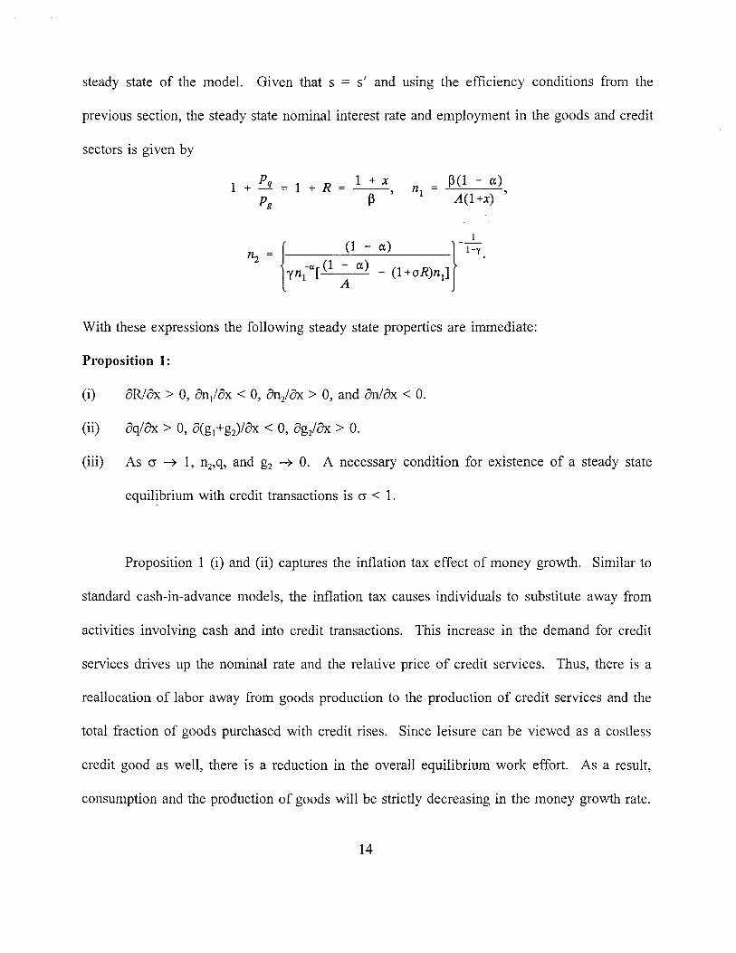
steady state of the model. Given that s = s’ and using the efficiency conditions from the
previous section, the steady state nominal interest rate and employment in the goods and credit
sectors is given by
1+~i=1+R=1~ ~3(1—a)Pg p ‘ 1 A(1+x)
= - - a)
A - (1÷oR)n13
With these expressions the following steady state properties are immediate:
Proposition 1:
(i) ER/ax> 0, ôn,/&x < 0, 0n2/~x>0, and anlox < 0.
(ii) aq/ox> 0, a(g,+g2)/ax < 0, ag2/ax> 0.
(iii) As a —~ 1, n2,q, and g2 —* 0. A necessary condition for existence of a steady state
equilibrium with credit transactions is a < 1.
Proposition 1 (i) and (ii) captures the inflation tax effect of money growth. Similar to
standard cash-in-advance models, the inflation tax causes individuals to substitute away from
activities involving cash and into credit transactions. This increase in the demand for credit
services drives up the nominal rate and the relative price of credit services. Thus, there is a
reallocation of labor away from goods production to the production of credit services and the
total fraction of goods purchased with credit rises. Since leisure can be viewed as a costless
credit good as well, there is a reduction in the overall equilibrium work effort. As a result,
consumption and the production of goods will be strictly decreasing in the money growth rate.
14

Proposition 1 (iii) says that in the limiting case where credit producers must finance all
of the household’s credit purchases with cash (a = 1), the model degenerates to a pure cash in
advance economy where all household transactions involve cash and the credit producing sector
vanishes. Intuitively, a can be viewed as a technological or institutional parameter which
measures how more efficiently credit producers can carry out transactions relative to households.
Since the cost of borrowing to credit producers is directly proportional to this parameter, their
profit maximizing choice ofemployment decreases with a. Also, since the steady state relative
price of credit services is exactly the nominal interest rate, it will never be optimal to hire labor
and supply credit services if credit producers are equally cash constrained as households in the
goods market. We will discuss further intuition behind a in an institutional context in the
quantitative exercises of Section IV.
B. Some Properties of the Stochastic Equilibrium
To analytically extract the liquidity effect of monetary shocks from the anticipated
inflation effects, let the stochastic process governing the money growth rate be i.i.d. Thus, the
transition density may be written as 1’(s,ds’) = D(ds’). The cash-constraints in (9) and (10)
gives p6[g1 + ~q] = {d(1-a) + a + x}/a. Substituting this into (23) gives
J (s) = a ~ (dy’) = j. (31)in JId(1—a) + ~ +xJ in
Notice that since d E (0,1) is chosen before the current state s’ is realized, it can be treated as
a constant in the decision rules ofthe other variables within the period. Equation (31) states that
this feature, combined with the i.i.d. nature of the monetary shock, implies that the marginal
value of an extra dollar for the family entering the current period will be constant. This result
15

will prove extremely useful in establishing the following proposition regarding the effect of an
unanticipated monetary shock.
Proposition 2. A positive innovation to the money growth rate
(i) increases the fraction of total household consumption purchased with credit,
(ii) increases employment and output in the goods producing and credit services sectors,
(iii) decreases the relative price of credit services to consumption goods.
Proof. From equation (10) p,, = (d+x)/aQ(n2). Substituting this and (18) into equation (16) and
rearranging gives
fd + Xl.j - AoQ(n2)+ xf in - F~(n1)
Substituting (30) into the above expression yields one equation which can be solved for n, as a
function of d, ~m’and x:
= ,~, a~3fa+ x + d(1-a)~ (32)tmAo~ 1+x J
Since a + d(1-a) < 1, it is immediate that employment and output in the goods producing sector
will be strictly increasing in the monetary shock. With this, the stochastic behavior ofn2 can be
easily characterized by substituting (32) into (30) and solving for Q(n2):
~ - d + x ~ aP(o + x + d(1-o)~ (33)2 o+x+d(1—o) [~~AOI~, 1 + x
Thus, employment and output in the credit producing sector increases with the size of the
monetary shock as well. These results imply that aggregate consumption and household work
effort will respond positively to the monetary innovation. Equation (26) implies that this leads
16

to a negative relationship between a positive money shock and the relative price of credit
services. ~
The intuition behind these results can be given by the following observations. Since the
household saving decision (d) must be made prior the realization ofthe current monetary shock,
monetary injections ofcash enter the economy asymmetrically through the financial sector and
credit producing firms. This creates a liquidity premium for producers of credit services who
must finance a portion of household purchases of credit goods with cash. As a result, credit
producing firms increase their demand for labor and expand the supply of credit services to
households. This drives the relative price of credit services as well as the nominal interest rate
down. Credit services are valuable to households because it permits them to circumvent the
inflation tax effects ofholding cash between periods (given a positive steady state money growth
rate). Households respond to this increased availability of credit services by increasing work
effort, the fraction of consumption financed with credit, and total consumption. As a result,
employment and output in both sectors respond positively to the current monetary injection.
IV. Quantitative Properties of the General Model
The previous section separated out both the pure anticipated inflation and liquidity effect
of a monetary injection in the household credit model. Since money growth rates consistent with
U.S. time series exhibit positive serial correlation both of these effects will be present. This
section investigates the cyclical properties of our general model and evaluates at some
quantitative level the importance of household credit markets in generating a dominant liquidity
effect. The model is solved using a linear-quadratic (L-Q) approximation technique that involves
17

linearizing Euler equations (27), (28), and (29) with a Taylor-series approximation about the
steady state. A method of undetermined coefficients is then used to solve for decision rules
which are linear in the model’s state variables. The money growth rate in the model will be
assumed to follow a stationary AR(1) process:
= (1 — p)x* + px~+ ~, (34)
where x~is the steady state value for x,, p < 1, and ~ is a white noise disturbance with zero
mean and constant variance.
Consistent with previous real business cycle studies [e.g., Cooley and Hansen (1989)] we
set a = 0.36, ~ = 0.99, and S = 0.025. The value of A = 2.55 is chosen to give a steady state
hours worked of 1/3. Aiyagari and Eckstein (1994) uses estimates ofthe production function for
credit services which finds y = 0.35. The money supply process parameters are set as x* = 0.016
and p = 0.32 based on Christiano (1991).~However, it is not immediately obvious how to select
an appropriate values for a. Recall that a measures the fraction of household credit purchases
that credit producers must finance with cash. Since in equilibrium a = (d+x)/p6g2, one possible
empirical counterpart to this is the ratio ofthe quantity ofcash deposited into the financial sector
to bank loans. Thus, a rough estimate for a may be inferred by looking at the ratio of total
reserves to demand deposits. This gives us a benchmark value of a = 0.15 and a starting point
7This figure, used as the benchmark parameters for Christiano (1990) and Fuerst (1993), is based
upon estimated money growth models for the post-1970 sub-sample
18

about which to conduct our sensitivity analysis.8 Finally ~ and k2 are set to 41.6 and 0.12,
respectively, so that the steady state value of pqQ/(pgY+pqQ) is 0.89%, the approximate value
added share of the U.S. household banking sector.9
Impulse response plots to a one time, one percent positive monetary shock for the cash-in-
advance (CIA) case, where d is chosen after x~is observed, as well as our household credit (HC)
model are presented in Figures 2A through 21. The shock occurs in period 10 and the vertical
axis for real variables measures percent deviations from steady state. Figure 2B shows that
employment in the credit producing sector increases for both models. This is since the
anticipated inflation effect increases household credit demand while the liquidity effect works to
increase the availability ofhousehold credit. Hence, the equilibrium quantity of credit services
in Figure 2D increases for both models.
However, the models have exactly the opposite predictions for the cyclical behavior of
employment in the goods producing sector, aggregate employment, consumption, investment, and
the nominal interest rate. Although money and credit services are positively related in CIA they
are also countercyclical. The anticipated inflation effect in CIA depresses employment and real
activity in the goods producing sector and raises the nominal interest rate. To the contrary, the
benchmark HC model displays a dominant liquidity effect where the nominal interest rate in
Figure 2G falls in the period ofthe shock. The expansion ofhousehold credit services increases
8 Source: Federal Reserve Bulletin, 1995. Alternative measures include the ratio of reserves to
consumer loans and reserves to transactions deposits (10 percent and 7.5 percent in 1996, respectively).Thus, a = 0.15 seems like a reasonable and “conservative” choice.
9The value added share of the banking sector [excluding insurance agents and services] is 2.7% ofGDP [see Diaz-Gimenez et.al. (1992)]. Actual household financial activity accounts for roughly 1/3 ofthis measure.
19

hours worked in both sectors as well as aggregate employment and investment and this leads to
a short-term boom in the industrial sector (Figures 2A, 2B, 2C, and 2F). Furthermore,
consumption in Figure 2E now rises in the period of the shock as well. Unlike the typical
liquidity effect model, the monetary injection is actually able to mitigate the inflation tax effect
by lowering the real cost of consumption through the availability of credit services.
Finally, Figures 2H and 21 compare the responses of the nominal rate (Ri) and relative
price of credit services (PR,) across CIA and HC models. Since the monetary shock is
anticipated when portfolio decisions are made, CIA predicts that both coincide and rise in the
period of the shock. Interestingly enough, while both falls in HC, the volatility of the nominal
rate exceeds that of the relative price of credit services. Intuitively, the monetary shock
unexpectedly increases the marginal value of cash in the goods market relative to the financial
market, making the opportunity cost of using cash, or the nominal rate, lower than that ofusing
credit services at the margin. This feature ofthe model may also help to explain the observation,
by some, that the cost of consumer borrowing tends to be “sticky” and less volatile than the
nominal interest rate.
To test the sensitivity ofthe size ofthe liquidity effect in the HC model to changes in the
fraction ofhousehold credit purchases which credit producers must finance with cash, alternative
values of a are considered. In addition to the our benchmark value, we consider higher values
of a = 0.25 and 0.30. Corresponding to each value of a we also choose an alternate value for
4’ so that the model’s steady state remains consistent with a 0.89 percent value added share ofthe
household credit sector. Figures 3A through 3G compares the impulse responses from these
cases to that of the benchmark model. These plots clearly show that the size of the liquidity
20

effect is strictly decreasing in the size of a. Otherwise, the behavior of hours worked,
consumption, investment, and credit services look similar to the patterns in Figure 2.
To understand the reasoning behind this result, consider the cash constraint on credit
producers given by (10). In equilibrium this constraint becomes pgq = (d+x)/a. Intuitively, 1/a
can be interpreted as a measure of how efficiently credit producers carry out transactions for
households. At a = 1 credit producers and households are equally cash constrained and hence
credit producers will have no incentive to supply credit services. Such a model degenerates to
a basic cash-in-advance model where all household transactions will involve cash. All else being
equal, (1/a) > 1 generates a “multiplier effect” by which a monetary injection expands the
availability of nominal credit services to households and hence the size of the liquidity effect.
Thus, as a falls the liquidity effect will begin to dominate the anticipated inflation effect. Notice
that this intuition also makes sense given our institutional interpretation of a. If we view it as
the total fraction of required and excess reserves in the banking system, it is reasonable to think
that the quantity of credit available in response to a monetary injection would be decreasing in
this ratio (with no credit services available in the extreme case of a = 100%).
V. Concluding Remarks
This paper has explored the role ofhousehold credit markets in explaining the observed
positive and procyclical relationship between money and credit services over the business cycle.
Monetary injections through financial intermediaries and credit producers were shown to generate
a liquidity effect by which real activity is influenced through an expansion of household credit
services. Our quantitative results also suggests that there does exist reasonable parameter values
21

where this effect may dominate the anticipated inflation effects of monetary growth.
Furthermore, the model is able to resolve one important difficulty with the basic Lucas-Fuerst
liquidity effect model. Because monetary injections increase the availability ofhousehold credit
services it is actually able to circumvent the inflation tax effect on consumption. Thus,
consumption responds positively to the monetary shock as well.
These results also provide a nice complement to recent liquidity effect models
emphasizing business credit as an important element in explaining the procyclical behavior of
money and the business cycle. However, similar to these models, our set-up also lacks a
persistent liquidity effect which is evident in U.S. time series. There are two possibilities to
pursue with this issue. First, one could add rigidities which prevent the immediate adjustment
ofhousehold funds in the periods following an unexpected monetary shock. Second, and perhaps
more interesting, is to explicitly analyze the behavior of consumer durable spending in this
model. This may not only contribute to the persistence issue but also help explain another
important empirical regularity. Over a typical business cycle household investment is procyclical
and leads the cycle while business investment lags the cycle. From causal observation, a
majority of consumer durables and residential investment is financed with credit as opposed to
cash. Thus, our household credit framework may be able to provide a monetary explanation of
this phenomena.
22

References
Aiyagari, S. Rao and Zvi Eckstein (1994). “Interpreting Monetary Stabilization in a Growth
Model with Credit Goods Production.” Working Paper 525, Federal Reserve Bank of
Minneapolis.
Ausubel, Lawrence (1991). “The Failure of Competition in the Credit Card Market.” American
Economic Review 81: 50-81.
Bernanke, Benjamin (1992). “Credit in the Macroeconomy.” Federal Reserve Bank ofNew York
Quarterly Review, Spring.
Bernanke, Benjamin and Alan Blinder (1992). “The Federal Funds Rate and the Channels of
Monetary Transmission.” American Economic Review 82: 901-21.
Boldin, Michael (1994). “Econometric Analysis of the Recent Downturn in Housing: Was it a
Credit Crunch?,” mimeo, Federal Reserve Bank ofNew York.
Christiano, Lawrence J. (1991). “Modeling the Liquidity Effect of a Money Shock.” Federal
Reserve Bank ofMinneapolis Quarterly Review, Winter.
Christiano, Lawrence J. and Martin Eichenbaum (1992). “Liquidity Effects and the Monetary
Transmission Mechanism.” American Economic Review 82: 346-53.
Christiano, Lawrence J. and Martin Eichenbaum (1995). “Liquidity Effects, Monetary Policy,
and the Business Cycle.” Forthcoming in Journal of Money, Credit, and Banking.
Cooley, Thomas F. and Gary D. Hansen (1989). “The Inflation Tax in a Real Business Cycle
Model.” American Economic Review 79: 733-48.
Cooley, Thomas F. and Gary D. Hansen (1991). “The Welfare Cost of Moderate Inflations.”
Journal of Money, Credit, and Banking 23: 483-503.
Diaz-Gimenez, Javier, Edward Prescott, Terry Fitzgerald, and Fernando Alvarez (1992).
“Banking in Computable General Equilibrium Economies.” Journal of Economic
Dynamics and Control 16: 533-559.
Duca, John (1995). “Credit Availability, Bank Consumer Lending, and Consumer Durables.”
Working Paper 95-14, Federal Reserve Bank of Dallas.
Fuerst, Timothy S. (1992). “Liquidity, Loadable Funds, and Real Activity.” Journal of
Monetary Economics 29: 3-24.
23

Fuerst, Timothy 5. (1993). “Liquidity Effect Models and their Implications for Monetary
Policy.” Working Paper, Northwestern University.
King, Robert G. and Charles Plosser (1984). “Money, Credit, and Prices in a Real Business
Cycle Model.” American Economic Review 74: 363-380.
King, Robert G., Charles Plosser, and Sergio Rebelo (1987). “Production, Growth, and Cycles:
Technical Appendix.” Manuscript, University of Rochester.
Lucas, Robert E. Jr. and Nancy L. Stokey (1987). “Money and Interest in a Cash-in-Advance
Economy.” Econometrica 55: 491-513.
Lucas, Robert E. Jr. (1990). “Liquidity and Interest Rates.” Journal of Economic Theory 50:
237-264.
Mester, Loretta J. (1994). “Why are Credit Card Rates Sticky?” Economic Theory 4: 505-530.
Park, Sangkyun (1993). “The Determinants ofConsumer Installment Credit.” Economic Review,
The Federal Reserve Bank of St. Louis (November): 23-38.
Stockman, Alan C. (1981). “Anticipated Inflation and the Capital Stock in a Cash-in-Advance
Economy.” Journal of Monetary Economics 8 (November): 387-93.
Wilcox, James (1990). “Nominal Interest Rate Effects on Real Consumer Expenditure.”
Business Economics (October): 31-37.
24

Figure 2A: Employment in Goods Producing Sector0.0084
0.0072
0.0060
0.0048
0.0036
0.0024
0.0012
0.0000
-0.00 1210
Figure 2B: Employment in Credit Producing Sector0.0320
0.0280
0.0240
0.0200
0.0 160
0.0120
0.0080
0.0040
0.0000
-0.0040
0.0084
0.0072
0.0060
0.0048
0.0036
0.0024
0.0012
0.0000
-0.00 12
0.0200
0.0175
0.0150
0.012S
0.0100
0.007S
0.0OS0
0.002S
0.0000
-0.0026
Figure 2C: Aggregate Employment
Figure 2D: Credit Services
3 17 24 3 10 17 24
3 10 17 24 3 10 17 24

.~LiR~ I
(I) ~
Ftr~ANc~AL
t~re~c~,-1E~oI4R~(~‘2~ +~
—3
(.1) E~ -c~- ~
~JA~ttAL~ t-~L_~] < —i-- tt~rE~He~rAw~(
ftc~oL~uEc J
Icr2e-~tr I
~fRL~
I
~ft ~ ~7-+
NA4 —
I—l
(.~

Figure 2E: Consumption Figure 2G: Nominal Interest Rate0.00030
0.00026
0.00020
0.000 15
0.000 10
0.00006
0.00000
-0.00005
0.0270
0.0240
0.0210
0.0 180
0.0160
0.0 120
0.0090
0.0060
0.00303 10 17 24
Figure 2F: Investment
2 9 16 23
0.0200
0.0175
0.0 150
0.0 126
0.0100
0.0076
0.0050
0.0026
0.0000
-0.00263 10 17 24

Figure 2H:0.02660
0.02646
0.02640
0.02636
0.02630
0.02626
Nominal Rate and Relative Price of Credit - CIA
Figure 21:0.0270
0.0240
0.0210
0.0180
0.0 150
0.0120
0.0090
0.0060
0.0030
3 10 17 24
Nominal Rate and Relative Price of Credit - HC
2 9 16 23

sigma ~0.1S
sigma ~O.2S
sigma ~O.3S
0.0200
0.0176
0.0 150
0.0 125
0.0100
0.0076
0.0060
0.0026
0.0000
-0.0025
Employment in Goods Producing Sector
it
‘II I1kt
0.0084
0.0072
0.0060
0.0048
0.0036
0.0024
0.00 12
0.0000
-0.00 12
Figure 3C: Aggregate Employment
sigma 0.15
sigma ~O.2S
sigma ~O.35
I~’I
‘Iv
I’
Figure 3A:0.0084
0.0072
0.0060-
0.0048
0.0036
0.0024
0.0012 -
0.0000 *
-0.0012
Figure 3B:0.0320
0.0280
0.0240
0.0200-
0.0160-
0.0 120
0.0080
0.0040
0.0000
-0.0040 -
— I III II I Ill II Ill II
3 10 17 24 3 10 17 24
Employment in Credit Producing Sector
sigma~O.1S —
sigma 0.25 — —
~II’“I
I! I
‘I
sigma 0.35 — —
-- ~-
Figure 3D: Credit Services
sigma 0.15
sigma 0.25
sigma 0.36
I’
Ii’~‘I~
I! ~I
3 10 17 24 3 10 17 24

Figure 3E: Consumption0.0270
0.0240
0.0210
0.0180
0.0 150
0.0 120
0.0090
0.0060
0.0030
Figure 3G: Nominal Interest Rate
0.0200
0.0175
0.0150
0.0125
0.0 100
0.0075
0.0050
0.0025
0.0000
-0.0026
Figure 3F: Investment
sigma 0.16
sigma 0.26
sigma 0.3S
I’
I~II, \%
I’
0.000300
0.000260
0.000200
0.000 150
0.000100
0.000060
0.000000
-0.0000503 11 19 27 2 9 16 23
3 10 17 24


