
Housing Supply Elasticity and Rent Extraction by State and
Local Governments
Rebecca Diamond∗
Stanford GSB
March 21, 2016
Abstract
Governments may extract rent from private citizens by inflating taxes and spending onprojects benefiting special interests. Using a spatial equilibrium model, I show that less elastichousing supplies increase governments’abilities to extract rents. Inelastic housing supply, drivenby exogenous variation in local topography, raises local governments’tax revenues and causescitizens to combat rent seeking by enacting laws limiting power of elected offi cials. I find thatpublic sector workers, one of the largest government special interests, capture a share of theserents through increased compensation when collective bargaining is legal or through corruptionwhen collective bargaining is outlawed.
∗I am very grateful to my advisors Edward Glaeser, Lawrence Katz, and Ariel Pakes for their guidance and support.I also thank Nikhil Agarwal, Adam Guren, Caroline Hoxby, Enrico Moretti, Kathryn Shaw, Juan Carlos SuarezSerrato, two anonymous referees, and participants at the Conference on Urban and Real Estate Economics, HarvardLabor Workshop, NBER Labor Studies, Stanford Public Economics Seminar, Stanford Institute for TheorecticalEconomics, and the Wisconsin Labor Seminar.
1

1 Introduction
The determinants and justification of the size of government has been a topic of heated debate in
recent years, as many states and localities face budgetary stress. Many theories of local govern-
ment depict a benevolent social planner who maximizes social welfare. In contrast, Brennan and
Buchanan (1980) present a controversial "Leviathan Hypothesis" of the public sector. Drawing on
the theory of the private sector monopolistic, they envision a government that seeks to exploit its
citizens by maximizing tax revenue that it extracts from the economy. They stress that "interjuris-
dictional mobility of persons in pursuit of fiscal gains" can discipline a rent-seeking government.
This hypothesis was the subject of much debate in the 1980s, with many empirical studies produc-
ing inconclusive and contradictory results (Oates (1985), Nelson (1987), Zax (1989). See Ross and
Yinger (1999) for a review).1
In this paper, I present a new approach to testing the Leviathan Hypothesis, and gauging its
economic magnitude. This paper develops a spatial equilibrium model where governments must
compete for residents to tax, and residents can "vote with their feet" by migrating away from
excessively rent extractive governments, in the spirit of Tiebout (1956). The model shows that
governments which preside over areas with less elastic housing supplies are more able to raise
taxes without providing taxpayers with additional government services. Intuitively, when housing
is supplied inelastically, the incidence of the local taxes will predominately fall on house prices.
Residents’utility losses from high taxes will be offset by utility gain from more affordably housing,
making the incentive to out-migrate much weaker. Even though households are perfectly mobile,
inelastic housing supply lowers their mobility in equilibrium and mutes the disciplining "vote-with-
your feet" mechanism.
These rents extracted from taxpayers can provide the government with additional funding to
increase government workers’ pay, hire additional employees, or more generally spend on items
which benefit the government, but not the general public. Exogenous variation in housing supply
elasticity provides a new identification strategy for measuring the economic importance of the
Leviathan Hypothesis. I empirically test the model’s predictions by first showing that per capita
tax revenue is higher in housing inelastic areas. I then analyze how these extra tax dollars get
spent on items such as increased public sector compensation and increased employment levels.
I then consider whether governments extract rents not only through formal taxation, but also
by increasing informal taxes such as bribes and corruption. Finally, I test whether private citizens
partially combat government rent seeking by enacting laws which limit the power of elected offi cials.
The paper begins by laying out a stylized Rosen (1979) Roback (1982) spatial equilibrium model
where state and local governments set taxes and the level of government services to maximize
government "profits," which can then be spent on government interests, such as an expanded
1The Leviathan Hypothesis predicts that, all else equal, if there are many small governments, they will be forcedto compete with each other for citizens to tax. This increased competition will discipline government rent seekingand shrink the size of government. Most of the previous empirical literature focused on the correlation betweendecentralization of government and the size of government.
2

workforce or higher government compensation. Residents in the model vote with their feet and not
at the ballot box to focus on the role of migration as a government disciplining mechanism.
The model shows that if state and local governments are using their market power to spend
tax dollars on government interests, their abilities to extract rents from their citizens is determined
by the equilibrium migration elasticity of private sector residents with respect to local tax rates.
Governments trade off the benefits of a higher tax with the cost that a higher tax will cause workers
to migrate away, leaving the government with a smaller population to tax.
Less elastic housing supplies increase governments’abilities to extract rent from taxpayers and
raise revenue. A tax hike by a government in an area with inelastic housing supply leads to a
small amount of out-migration. Housing prices sharply fall due to the decrease in housing demand
driven by the tax hike. Thus, governments in housing inelastic areas can charge higher taxes
without shrinking their tax base since housing price changes limit the migration response. Further,
the model shows that governments’market power to raise taxes due to inelastic housing supply
remains even when there are a large number of governments competing for residents and every
government is small (Epple and Zelenitz (1981)).
When state and local governments exercise more market power in areas with inelastic housing
supplies, government spending should be more channelled toward items in the government’s interest.
In particular, the high unionization rate in the public sector may allow union bargaining to influence
the decisions of elected offi cials (Freeman (1986)). I analyze whether these effects are stronger in
states which have legalized public-sector collective bargaining.
I proxy for a metropolitan areas’s housing supply elasticity using data from Saiz (2010) on
the share of land within 50km of a city’s center unavailable for real-estate development due to
geographic constraints, such as the presence of swamps, steep grades, or bodies of water.2
Using county level data from the Census of Governments, I find that government revenue and
taxes levied per county resident are higher in housing inelastic areas, consistent with the Leviathan
Hypothesis. Further, I find these additional funds flow to increased government payroll per county
resident, the number of full-time equivalent (FTE) government workers per county resident, and
average government workers’wages.
Increased rent extraction could lead citizens to push back against these forces and place limits
on elected offi cials’powers. Indeed, I find that less elastic housing supply leads to shorter term
limits for elected offi cials and that citizens are more able to directly legislate at the ballot box
through local initiatives and referendums.
In addition, I find substantially different government spending effects across states depending
on whether public sector collective bargaining is legal.3 A one standard deviation increase in land
2With less available land around to build on, the city must expand farther away from the central business areato accommodate a given amount of population, driving up average housing costs. A full micro-foundation of thismechanism can be derived from the Alonso-Muth-Mills model (Brueckner (1987)) where housing expands around acity’s central business district and workers must commute from their house to the city center to work.
3Data on public sector collective bargaining laws were collected by Freeman and Valletta (1988). Hoxby (1996)uses these data to identify the effects of teachers unions on many aspects of education production. She uses variationin the timing of states’legalization of public-sector collective bargaining. Frandsen (2011) also uses these law changes
3

unavailability raises government wages by 4.2% in states which allow public sector bargaining, but
has little to no effect on government employment levels. However, in states which outlaw public
sector collective bargaining, a one standard deviation increase in land unavailability raises per
capita government employment by 1.8%, and has essentially no impact on government wages.
To further analyze whether government workers are receiving excess compensation in areas
with less elastic housing supplies, I quantify how the public-private sector wage gap varies across
metropolitan areas using data from the 1995-2011 Current Population Survey Merged Outgoing
Rotation Groups (CPS-MORG). Results from the CPS-MORG show a one standard deviation
increase in land unavailability raises the local public-private sector wage gap by 3.6% when public
sector collective bargaining is legal. Drilling down to specific occupations, I find especially large
effects for police and firemen wages, but little effect on teacher wages. This is similar to Frandsen
(2011)’s findings that the direct effect of these bargaining laws seems to raise police and fire fighters
wages more than teachers wages. Overall, state and local governments appear to excessively spend
on workforce compensation when they are able to raise additional tax revenue.
These findings are consistent with previous work by Brueckner and Neumark (2014), which
addresses a similar question of how desirable local amenities give state and local governments
taxation market power. They analyze how public-private sector wage gaps vary across states with
differing levels of desirable amenities, finding amenities increase the public-private sector wage gap
more in states permitting public-sector collective bargaining. Work by Feiveson (2011) finds that
federal government transfers to state and local governments largely get spent on higher government
wages in states where public sector collective bargaining is legal. However, a larger share of this
money goes to increased government employment in states outlawing bargaining. I find a similar
split of money between wage and employment growth.
Recent work by Bai, Jayachandran, Malesky, and Olken (2013) shows that the threat of out-
migration also disciplines government corruption and bribes. They study government bribes in
Vietnam and show that when firms are more likely to migrate away from corrupt areas, the level
of government bribes is lower. I test this mechanism in the US context by analyzing data from
the U.S. Department of Justice on the number of public corruption convictions by the presiding
federal district court in each geographic area.4 I find that a one standard deviation increase in
land unavailability increases public sector corruption by 40% within states which outlaw public
sector collective bargaining. However, states permitting collective bargaining have no increase in
corruption in housing inelastic areas.
It appears collective bargaining may give government workers a formal mechanism to bargain
for their share of rents from taxation and receive increased compensation. However without this
bargaining mechanism, workers may turn to informal ways of capturing these rents through bribes
and corruption. Indeed, corruption convictions are 16% lower in states permitting collective bar-
gaining than those which outlaw it. Collective bargaining could potentially help keep corruption
to look at their effects on other types of government workers, including firefighters and police.4Since these are convictions in federal courts, the enforcement rate and funding of these courts cannot be influenced
by local revenue generated by inelastic housing supply.
4

in check by providing formal mechanisms to bargaining for rents.
The magnitudes of these effects are substantial. To put these estimates into context, consider
the differences in land unavailability between San Francisco, CA and St. Louis, MO, which both
permit public sector collective bargaining. San Francisco is surrounded by water to the north,
west, and east and contains steep grades. St. Louis is surrounded by open land, but has a river
running through the middle of the city. In the context of my measure, San Francisco’s land
unavailability is 2.9 standard deviations higher than St. Louis’. According to the 2007 census of
governments, the average San Francisco city employee earned $84,300 per year and likely received
benefits worth $42,150.5 My estimates imply that if San Francisco had the amount of land available
in St. Louis it could save $11,055 per city worker, for a total savings of $309 million per year.6 This
is equivalent to 12.8% of the total tax revenue collected by San Francisco.7 While there is little
hope for changing the topography of San Francisco to that of St. Louis, these numbers show that
government policies impacting housing supply can have economically large effects on government
spending. In particular, the rise in local land use regulation across US cities since the 1970s likely
has led to increased government rent extraction.
The paper proceeds as follows. Section 2 discusses the relation to previous literature. Section
3 layouts of the model. Section 4 presents empirical evidence, and Section 5 concludes.
2 Relation to Previous Literature
The labor literature studying public-sector compensation has also found evidence suggesting gov-
ernment jobs offer rents beyond the compensation of similar private sector jobs. Recent work
by Gittleman and Pierce (2012) find that the average public sector employee is more generously
compensated than a similarly qualified private sector employee. Although, the magnitude of this dif-
ference depends strongly on what covariates, such as occupation, are included as controls. Krueger
(1988) finds that there are more job applications for each government job than for each private
sector job, suggesting that government jobs are more desirable to workers, on average. Average job
quit rates reported from the 2002-2006 Job Openings and Labor Turnover Surveys show that the
average annual quit rate is 28% for private sector workers, but only 8% for public sector employees.
5The census of governments does not report spending on worker benefits, but Gittleman and Pierce (2012)’sanalysis of Employer Costs for Employee Compensation Survey shows that the average local government workerreceives benefits worth 50% of annual wage compensation. This suggests San Francisco employees receive $42,150 inbenefits.
6This assumes the local private sector wage does not respond to the increased housing supply elasticity. Increasingthe housing supply should lower rents and lead to lower equilibrium private sector wages. Since the rent extraction isa function of the public-private wage gap, this decrease in private sector wages would lead to additional governmentcost savings not accounted for in this calculation.
7 I calculate the wage savings as: 84,300-(exp(ln(84,300)-(.0359)*(2.9)))=$8335. The benefits saving are: 42150-(exp(ln(42150)-.023*(2.9)))=$2720, where I assume my estimated effects on health insurance spending can be gener-alized for all benefits spending. This leads to a total savings of $11,055 per worker. I multiply this by the number ofFTE wokers in San Fransicso in 2007 as reported in the Census of Governments (27,981), giving an annual savingsof $309 million. Total taxes collected by San Francisco in 2007 as reported by the Census of Governments was $2.41billion.
5
This paper shows that an increase in governments’abilities to extract rent directly leads to higher
government payrolls and benefits expenditures.
The public sector workforce is also highly unionized, enabling government employees to bargain
for rents. Gyourko and Tracy (1991) use a spatial equilibrium model to show that if the cost of
government taxes to citizens are not completely offset by benefits of government services, they will
be capitalized into housing prices. Similarly, if high levels of public sector unionization lead to
more government rent extraction, the public sector unionization rate will proxy for government
waste and also be capitalized into housing prices. Gyourko and Tracy (1991) find evidence for both
of these effects, however they need to assume the variation in taxes and unionization rates across
localities is exogenous. This paper uses land unavailability as a source of exogenous variation in
government market power to show collective bargaining laws allow governments to take advantage
of their market power to increase compensation.
As previously mentioned, my analysis builds on recent work by Brueckner and Neumark (2014)
(BN) who analyze an alternative mechanism through which state and local governments gain tax-
ation market power: the availability of desirable consumption amenities. They use a similar setup
where profit maximizing governments compete for residents by setting local tax rates. They allow
local governments to play a game in tax-competition where the number of competing governments is
small. I allow each government to be small when deriving the determinants of market power, which
I believe accurately captures the nature of competition between the over 89,000 local governments
in the US. They show that more desirable amenities are associated with higher public-private wage
gaps. When I control for the impacts of amenities used by BN, I continue to find evidence for the
role of inelastic housing supply in government rent seeking. Further, I empirically identify these
effects on local taxes, government employment levels, benefits, corruption, and voters’ reactions
through legislation, while BN primarily focuses on public sector wages. These many outcomes to-
gether help illustrate the causes of rent extraction, how these rents get distributed, and mechanisms
through which the private sector can fight against these forces.
3 Model
The model detailed below uses a Rosen (1979) Roback (1982) spatial equilibrium to analyze how
local governments set taxes, employ workers, and compete for residents. In the model, I assume
that governments use a head tax to collect revenue, however in reality, most state and local gov-
ernments use property and income tax instruments. In Appendix A I derive results for the case of
a government income or property tax and show the same results. I also abstract away from the po-
litical election process in each area. While politics could surely influence the extent of government
rent seeking, my goal is to analyze the disciplining effects of migration on government rent seeking.
The nationwide economy is made up of many cities. There are N cities, where N is large. Cities
are differentiated by their endowed amenity levels Aj ,which impact how desirable workers find the
city, and their endowed productivity levels θj , which impact how productive firms are in the city.
6

Workers are free to migrate to any city within the country. Each city has a local labor and housing
market, which determine local wages and rents. The local government provides government services
by employing workers and collects taxes.
3.1 Government
The local government of city j charges a head tax τ j to workers who choose to reside within the
city. The local government also produces government services, Y Gj , under the production function:
Y Gj = αjGj ,
where Gj is the number of government workers and αj is the exogenous productivity level of
government in city j. These government services are equally distributed across all workers in the
city, making each worker consume αGjNj units of government services. To simplify exposition, define
sj =αGjNj as the per worker amount of government services in city j. Nj measures the population of
city j. Since labor is the sole factor input, the cost of government service production is simply the
wage bill. For now, I will assume government workers are not unionized and earn their marginal
product of labor. In section 3.7 I will consider the case when workers unionize. In both cases, the
government is small relative to the overall labor market, making it a wage taker. The government
revenue and cost are:
Revenuej = τ jNj
Costj =wjsjNj
αj.
wj is the rate wage in city j. The local government is not benevolent and maximizes profits. These
profits could be spent on ineffi cient production of sj (thus, making the government benevolent,
but naive). They could also be directly pocketed by government workers, such as through union
negotiations. I will return to this case in section 3.7. For now, I assume the profits do not impact
government worker wages. The local government maximizes:
maxτ j ,sj
τ jNj −wjsjNj
αj
3.2 Workers
All workers are homogeneous. Workers living in city j inelastically supply one unit of labor, and
earn wage wj , either in the public sector or private sector. Each worker must rent a house to live in
the city at rental rate rj and pay the local tax τ j .Workers value the local amenities as measured by
Aj .The desirability of government services sj is represented by g (sj) , where g′ (sj) > 0, g′′ (sj) < 0.
Thus, workers’utility from living in city j is:
Uj = wj − rj +Aj + g (sj)− τ j .
7
Workers maximize their utility by living in the city which they find the most desirable.
3.3 Firms
All firms are homogenous and produce a tradeable output Y.Cities exogenously differ in their
productivity as measured by θj . Local government services impact firms productivity, as measured
by b(sj), where b′ (sj) > 0, b′′ (sj) < 0. The production function is:8
Yj = (θj + b(sj))NPj .
NPj is the number of workers in the private sector. The total size of the labor market equals
the sum of the public sector and private sector employment: Nj = NPj + Gj .The labor market is
perfectly competitive, so wages equal the marginal product of labor:
wj = θj + b(sj)
3.4 Housing
Housing is produced using construction materials and land. All houses are identical. Houses are
sold at the marginal cost of production to absentee landlords, who rents housing to the residents.
The asset market is in long-run steady state equilibrium, making housing price equal the present
discounted value of rents. Housing supply elasticities differ across cities. Differences in housing
supply elasticity are due to topography as well as other unobserved factors, which makes the
marginal cost of building an additional house more responsive to population changes (Saiz (2010)).
The housing supply curve is:
rj = aj + γj log (Nj) ,
γj = γxhousej
where xhousej is a vector of city characteristics which impact the elasticity of housing supply, includ-
ing topography.9
3.5 Equilibrium in Labor and Housing
Since all workers are identical, all cities with positive population must offer equal utility to workers.
In equilibrium, all workers must be indifferent between all cities. Thus:
Uj = wj − rj +Aj + g (sj)− τ j = U .
8 I assume a perfectly elastic labor demand curve to focus on the role of housing supply elasticity and keepexpressions simple. A downward sloping labor demand curve can be added without changing the results.
9See Saiz (2010) for a full micro-foundation of this housing supply curve.
8

Plugging in labor demand and housing supply gives:
θj + b(sj)− aj − γj logNj +Aj + g (sj)− τ j = U . (1)
Equation (1) determines the equilibrium distribution of workers across cities.
3.6 Government Tax Competition
Local governments set city tax rates and the level of government services to maximize profits, taking
into account the endogenous response of workers and firms in equilibrium, equation (1). Each city
is assumed to be small, meaning out-migration of workers to other cities does not impact other
cities’equilibrium wages and rents. If there were a small number of cities, each city would have
even more market power than in this limiting case. The results below can be thought of as a lower
bound on the market power of local governments competing for residents. They maximize:
maxsj ,τ j
τ jNj −wjsjNj
αj.
The first order conditions are:
0 = τ j∂Nj
∂sj− wjNj
αj− wjsj
αj
∂Nj
∂sj(2)
0 = τ j∂Nj
∂τ j+Nj −
wjsjαj
∂Nj
∂τ j.
Differentiating equation (1) to solve for ∂Nj∂sj
and ∂Nj∂τ jgives:
∂Nj
∂sj=
b′ (sj) + g′ (sj)(γjNj
) > 0
∂Nj
∂τ j=
−1(γjNj
) < 0. (3)
Population increases with government services and decreases in taxes. Plugging these into (2) gives:
0 =
(τ j −
wjsjαj
)b′ (sj) + g′ (sj)(γjNj
)−Nj
τ j = γj +wjsjαj
.
9

Combining the first order conditions shows that government services are provided such that the
marginal benefit (b′ (sj) + g′ (sj)) per resident equals marginal cost per resident(wjαj
):
b′(s∗j)
+ g′(s∗j)
=wjαj. (4)
This is the socially optimal level of government service.
The equilibrium tax rate is:
τ∗j = γj + s∗j . (5)
The elasticity of city population with respect to the tax rate(εmigratej
)can be written as:
εmigratej =∂Nj
∂τ j
τ jNj
.
Plugging in equation (3) for ∂Nj∂τ j
and rearranging gives:
(γj)
=−τ j
εmigratej
.
Substituting this expression into the equation (5) shows that the tax markup can be written as a
standard Lerner Index:τ∗j − s∗jτ∗j
=−1
εmigratej
.
The tax markup above cost is equal to the inverse elasticity of city population with respect to the
tax rate. While workers are perfectly mobile between cities, worker migration causes shifts along
the local housing supply curves. An increase in local taxes would cause workers to migrate to other
cities. A decrease in population will cause rents to fall, by moving along the housing supply curve.
This decrease in rents will increase the desirability of the city to workers, limiting the migration
response to the tax increase. The government takes into account the equilibrium rent response
to a tax hike when setting taxes to profit maximize. Thus, if migration leads to large changes in
local rent, a tax increase will not lead to large amounts of out-migration, since workers will be
compensated for the tax with more desirable rents.
To analyze the effect of housing supply elasticity on governments’ability to extract rent from
taxes, I differentiate the tax markup with respect to the slope of the inverse housing supply curve,
γj .∂
∂γj
(τ∗j − s∗j
)= 1 > 0. (6)
Equation (6) represents the increased rent response to migration induced by a tax hike in a city with
an inelastic housing supply. The equilibrium condition, equation (1) , shows that out-migration will
continue until the negative utility impact of the tax hike has been completely offset by changes in
10

the city’s wage and rent. In a city with a less elastic housing supply, a smaller amount of migration
is needed to push housing rents down to offset the negative utility impact of the tax hike. The
government can extract more rent through higher taxes in a city with a less elastic housing supply.
Note that this result assumes there are a large number of cities. Cities can extract rent even in
an environment where there are a large number of competitors because household demand for city
residence can never be infinite in equilibrium.
Additionally, this model assumes cities charge a head tax, while in reality most cities and states
tax their population through income taxes and property taxes. The amount of rent extraction
depends on the elasticity of tax revenue with respect to the tax rate. Thus, an income tax will
depend both on the wage response to the tax rate, as well as the migration response. Appendix A
shows that when using an income tax, governments can still exercise more market power in housing
inelastic areas.
In the case of a property tax, government revenue will depend on the local rental rate and
the size of the tax base. An increase in the property tax rate can decrease government revenue
both by incentivizing workers to migrate away, shrinking the tax base, and decreasing housing
rents, lowering tax revenue from each household. However, I show in Appendix A that the housing
supply elasticity will not impact the size of the rental rate decrease in response to a given tax hike.
Recall the equilibrium condition, equation (1) . For workers to derive utility U from a local area, the
utility impact of a tax increase must be perfectly offset by a rent decrease. Thus, the equilibrium
rental rate response to a given tax increase does not depend on the local housing supply elasticity.
Indeed, the housing supply elasticity determines the migration response required to change housing
rents in order to offset the utility impact of the tax increase. Thus, a less elastic housing supply
decreases the elasticity of government revenue with respect to the tax rate, giving the government
more market power when using a property tax instrument. See Appendix A for the full derivation
of this result.
Regardless of the tax instrument, governments of cities with less elastic housing supplies are
able to extract more rent from their residents.
3.7 Public Sector Unionization
The previous section assumed the government workers had no market power and were wage takers.
This lead the public and private sector wages to be identical in equilibrium and for workers to
be indifferent between employment in the public and private sectors. If public sector workers are
unionized, they could be able to bargain for a share of the rents earned by the government and
increase their compensation. Let λ be the share of the rents captured by the public sector union.10
The total rents extracted by the government is city j are γjNj . I assume this gets equally split
10 I assume that λ is small and does not impact the profit maximization decision of the overall government rentextraction.
11

across all public sector workers, in addition to the wage they would receive in the private sector:
wunionj = wj +λγjNj
Gj. (7)
Re-writing the public sector labor demand, in terms of the optimal amount of per household
consumption of government services, s∗j , :
Gj =s∗jNj
α,
I can plug this into the union wage equation (7):
wunionj = wj +αλγjs∗j
.
It clear to see that union public sector wages are increasing in γj , the slope of the inverse housing
supply curve.∂wunionj
∂γj=αλ
s∗j> 0.
Note that s∗j does not depend on housing supply elasticity, as shown in equation (4).
The model predicts that the rents due inelastic housing supply only flow to government workers’
wages when workers can collectively bargain. In this world, all workers would strictly prefer to
work in the public sector than the private sector, leading to job rationing. In the next section, I
empirically test these predictions.
4 Empirical Evidence
4.1 Government Revenue Regressions
The model predicts that local governments in areas with less elastic housing supplies will be able
to extract more rent from their residents. Saiz (2010) shows that the topological characteristics of
land around an MSA’s center impact whether the land can used for real-estate development. Cities
located next to wetlands, bodies of waters, swamps, or extreme hilliness have limits on how many
buildings can be built close to the city center, which impacts the elasticity of housing supply to
the area. Saiz (2010) uses satellite data to measure the share of land within 50km of an MSA’s
center which cannot be developed due to these topological constraints. A rent-seeking government
is able to charge higher taxes in areas with less land available for development. I z-score the MSA
level data from the land unavailability measure and use it as measures of cities’housing supply
elasticities. Table 1 reports summary statistics on these measures. The data cover 47 states (there
is no data for Hawaii, Alaska, or Wyoming) and 269 MSAs.11
11 I also aggregate these measures to a state-level index for cross-state analysis, where I weight each MSA measureby the state population in each MSA. The state-level housing supply elasticity measure is a noisy measure of the
12

I directly test this prediction by analyzing how local government revenue and taxes vary with
characteristics which impact local housing supply elasticities. I measure total revenue and taxes
from the 1962-2002 Census of Governments County Area Finance data. These data report every
five years on all local governments within a county. This includes the county government, as well
as the municipalities, townships, school districts, and special districts within the county.12 Table
1 Panel A reports summary statistics on average log county area total revenue and taxes collected
per county resident.13 I include only the counties within the metropolitan statistical areas covered
by Saiz’s land unavailability data, since these are the counties used in the regression analysis.
To test the model’s predictions, I estimate the following regression:
lnYjt = αt + βelastzelastj + εijt. (8)
Yijt measures the government revenue outcome of interest in county i in MSA j in year t. zelastj
measures MSA j’s level of land availability. As controls, I include year fixed effects, αt. Standard
errors are clustered by MSA since there is MSA-level variation in housing supply elasticity. The
model predicts that revenue and taxes should be higher in areas with less elastic housing supplies:
βelast > 0.
Consistent with the model, Panel A of Table 2 shows a one standard deviation increase in land
unavailability increases per capita government revenues by 8% and total taxes collected by 8.6%.
Local governments are capturing the benefits of inelastic housing supply.
4.2 Government Spending Regressions
While this extra money could be spent in a number of ways, it is possible some of it goes to
government payrolls, either by expanding the workforce or raising wages. These effects could be
especially strong in states where public sector collective bargaining is legal. These unions may
be able to better channel the government’s taxation market power into spending that benefits
government workers since they have an explicit mandate to represent the interests of government
employees.
I measure local government payrolls, employment, and wages using data from the 1972-2007
Census of Governments County Area Employment data. Table 1 Panel A reports summary statistics
on average log county area payroll, employment, and number of full-time equivalent government
workers per county resident. Average county-area government wages are calculated by dividing
total government payrolls by number of full-time equivalent government workers.
Consistent with the model, Panel B of Table 2 shows a one standard deviation increase in an
MSA’s land unavailability increases government payrolls per county resident by 4.8%, increases
overall housing supply elasticity for the state, since the data is only based off of the MSAs covered by Saiz’s sample.12County area finance data for 2007 has not been made available at this time.13Tax revenue is a subset of total revenue collected.
13
government full-time equivalents per county resident by 1.3% and increases average government
worker wages by 3.5%.
To assess whether collective bargaining impacts how much extra spending goes to the gov-
ernment workforce, I interact the land unavailability measure with whether the state allows local
government workers to collectively bargain. The dataset on public sector collective bargaining laws
was originally constructed by Richard Freeman and Robert Valletta in 1985 (Freeman and Valletta
(1988)), and codes the relevant laws for every state and every year from 1955 to 1985. This dataset
was later extended by Kim Rueben to cover the years through 1996. This paper uses the extended
Rueben dataset, filling forward the 1996 data through years 1997-2007. These laws have been
quite stable during this period, barring the very recent law changes in the last quarter of 2011 in
Wisconsin, which is beyond the range of the dataset.
While state laws vary in their exact provisions for public sector collective bargaining, I place
the laws into two categories: collective bargaining is prohibited or collective bargaining is either
permitted or required. The prohibited category includes statutes which explicitly prohibit state
employers from bargaining with worker representatives, but also situations where state law makes
no provision for collective bargaining, since courts have typically interpreted this as prohibiting
collective bargaining (Freeman and Valletta (1988)). The permitted or required category includes
states which authorize the employer to bargain and which give employee organizations the right to
present proposals or meet and confer with the employer, as well as those states which either imply
or make explicit the duty of the employer to bargain.
The data contain information on bargaining laws explicitly for teachers, police, and firefighters,
as well data on laws for other local government workers. I use the law data for "other local govern-
ment workers" for analyzing the impacts on these aggregate government spending measures. Table
1 Panel C reports summary statistics on these collective bargaining laws. Adding in interactions
of land unavailability with the collective bargaining laws gives the estimating equation:
lnYjt = αt + βbargzbargjt + βelastzelastj + βelast_bargzelastj ∗ zbargjt + εijt.
zbargjt is a dummy for whether public sector collective bargaining was legal in county j in year t.
This analysis of collective bargaining laws uses cross-sectional variation in the legality of collective
bargaining to identify its impact on government rent-seeking. Frandsen (2011) shows that cross-
sectional estimates of the direct impact on collective bargaining on public sector wages tend to be
higher than estimates which use longitudinal changes in state laws overtime. While this suggests
there may be omitted variables correlated with collective bargaining laws that impact government
worker wages, this paper’s analysis looks at how these laws interact with land unavailability. While
I cannot rule out the presence of omitted variables, they would have to interact with land unavail-
ability in how they impact government wages, payrolls and employment to cause bias. Further,
Frandsen (2011) shows using longitudinal variation in law changes as an alternative identification
strategy is also confounded by trends in states’government wages over time. Using variation in law
changes also requires getting data going back to the 1960s. Thus, using cross-sectional variation
14

in collective bargaining laws interacted housing supply elasticity can provide strongly suggestive
evidence of a causal channel, but surely cannot fully eliminate all potential omitted variable biases.
Table 2 shows that in states which allow public sector collective bargaining, a one standard
deviation increase in land unavailability increases government payrolls per county resident by 5.4%,
while it only increases payrolls by 1.3% in states which outlaw public sector collective bargaining.
Further, this estimate for states which prohibit bargaining is not statistically significant. While
these estimates cannot rule out small effects of housing supply elasticity on government payrolls in
places which prohibit bargaining, there appears to be quite large, positive effects where bargaining
is legal.
Turning to the effects on employment levels, a one standard deviation increase in land un-
availability in states prohibiting public sector collective bargaining raises the number of full-time
equivalent workers per county resident by 1.8%, and by 1.2% in states outlawing bargaining. How-
ever, the estimates are too noisy to say whether these effects differ based on legality of collective
bargaining.
Column 6 of Panel B in Table 2 shows the impact of land unavailability on average government
wages in states with and without public sector collective bargaining. Housing supply elasticity
has essentially no impact on government wages when bargaining is prohibited. The point estimate
shows a one standard deviation increase in land unavailability lowering wages by 0.48%, but the
effect is not statistically significant. However, in states which allow bargaining, land unavailability
raises wages by 4.2%. Thus, collective bargaining appears to take advantage of areas’ housing
supply elasticity market power and raise government payrolls, with essentially all of this extra
spending going to higher government wages. In areas where collective bargaining is prohibited,
government employment levels appear to slightly increase and may also slightly raise government
payrolls to pay for this increase.
To gain further insight into how these local governments elect different expenditures, I redo
these analyses within 19 categories of government spending. The effects do not appear to be driven
by specific types of government workers. See Appendix B for more details.
Since the role of housing supply in government spending decisions differ significantly based on
collective bargaining, I also check whether government revenues and taxation also differ by collective
bargaining laws. Columns 3 and 4 of Panel A of Table 2 shows that the land unavailability effects
on revenues and taxes do not statistically differ between states which do and do not allow public
sector collective bargaining. However, the point estimates are slightly higher in state permitting
bargaining.
Whether governments pass on their additional tax revenue to governments workers appears
to depend on whether public sector workers can collectively bargain. However, higher average
government wages does not necessarily mean that these government workers are getting "over
paid." It is possible that workers in these housing inelastic areas are more skilled and thus deserve
a higher wage. In addition, it could be that the market wage for workers is higher in these housing
inelastic areas, thus forcing the local governments to spend more on government wages. To test
15
these theories, I turn to data from the Current Population Survey so that I can directly control
for workers’demographic and skill differences, as well as use private sector worker wage data to
control for MSA differences in market wages.
4.3 Wage Gap Regressions
In this analysis, I focus on public-private sector wage gaps across MSAs as a measure of excess
compensation to government employees. By comparing the wages of government workers living
in a given MSA to similarly qualified private sector workers living in the same area, I control for
differences in market wages across MSAs, which could have confounded the previous analysis of
the Census of Governments wage data. To measure public-private sector wage gaps across MSAs
and states, I use data from the Current Population Survey Merged Outing Rotation groups from
1995-2011.14 The CPS-MORG is a household survey which collects data on a large number of
outcomes including workers’weekly earnings, hours worked, public/private sector of employment,
union status, and a host of demographics. I restrict the sample to 25 to 55 year old workers with
positive labor income, working at least 35 hours per week, to have a standardized measure of weekly
earnings. The CPS’s usual weekly earnings question does not include self-employment income so all
analysis excludes the self-employed. I also restrict analysis to workers whose wages are not imputed
to avoid any bias due to the CPS’s wage imputation algorithm (Bollinger and Hirsch (2006)). I
measure earnings using workers’log usual weekly earnings, deflated by the CPI-U and measured
in real 2000 dollars. Top coded weekly earnings are multiplied by 1.5 and weekly earnings below
$128 are dropped from the analysis.15 All analysis is weighted by the CPS earnings weights.
Table 1 reports summary statistics of workers’log weekly earnings each for workers employed in
the private sector, local government, state government, and federal government.16 Consistent with
previous works, such as Gittleman and Pierce (2012), the raw earnings are higher for all three classes
of government workers than for private sector workers. However, these raw earnings differences do
not account for differences in the characteristics of workers between the public and private sector.
To test the model’s predictions, I will control for worker characteristics when evaluating differences
in the public private sector wage gap. Additionally, the CPS only collects data on workers’earnings,
but not compensation paid to workers in the form of benefits. Gittleman and Pierce (2012) show
using the BLS’restricted-use Employer Cost of Employee Compensation microdata that government
employees receive significantly more generous benefits than similar workers in the private sector. I
will return to the question of benefits compensation, but first focus on public-private sector wage
14Since there was a significant change in the CPS’s earnings questions in 1994, I restrict analysis to 1994-2011.I also focus my analysis on workers whose wages are not imputed in the CPS. Since sector, occupation, and unionstatus are not used in the CPS’s imputation algorithm, analyzing government wage gaps and union wage gaps usingimputed wages can be problematic (Bollinger and Hirsch (2006)). Thus, I focus only on the non-imputed wagesample. The data flagging which wages were imputed are missing in the 1994 data, so I drop this year, leaving mewith a 1995-2011 sample.15 I follow Autor, Katz, and Kearney (2008)’s top and bottom coding procedures. Autor, Katz, and Kearney (2008)
drops all reported hourly wages below $2.80 in real 2000 dollars. This translates to $128 per week in real 2011 dollars,assuming a 35 hour work week. They also scale top coded wages by 1.5.16A worker’s sector is measured by the CPS variable reporting a worker’s class.
16

gaps.
To test the model’s predictions, I estimate the following regression:
lnwijt = δj + αt + βgovgovit + βelastzelastj ∗ govit + βXit + εijt. (9)
As controls, I include location fixed-effects δj , year fixed effects, αt, and a set of worker demograph-
ics which include 15 dummies for education categories, gender, race, Hispanic origin, a quartic in
age, and a rural dummy. govi is a dummy for whether the worker is government worker, zelastj mea-
sures land unavailability. Standard errors are clustered by state when using state-level measures
of housing supply elasticity and clustered by MSA when using MSA variation in housing supply
elasticity.
The nationwide average public-private wage gap is measured by βgov.The model predicts that
public-private wage gap should be higher in areas with less elastic housing supplies:
βelast > 0.
I test this prediction first using a sample including private sector workers and state government
workers. The state-level measure of land unavailability is calculated from a population weighted
average of MSA land unavailability within each state. There is likely more measurement error in
this state-level measure than in the MSA-level land unavailability measure since it does not include
data on the topography of cities and town outside of these MSAs within the state. Assuming this
mis-measurement is classical measurement error, the state-level estimates will be biased towards
zero.
Column 1 of Table 3 shows that the nationwide average wage gap between state government
employees and private sector workers is -0.112 log points. Consistent with Gittleman and Pierce
(2012), after controlling for worker demographics, government workers’ earnings are lower than
similar private sector workers, on average. However, the state worker-private sector wage gap
increases by 0.027 log points in states with a 1 standard deviation increase in land unavailability.
This effect is significant at the 5% level. Column 2 of Table 3 adds 3-digit occupation codes
interacted with a government employee dummy as additional controls. The effects are essentially
unchanged, showing that the public-private wage gap is not driven by differing occupation mixes
in the public or private sector related to land unavailability.
I now add in interactions with laws on whether state workers are allowed to collectively bargain.
While the cross-sectional variation in public sector collective bargaining laws is surely non-random,
the variation of interest is the relationship between land unavailability and government wages within
each category of state: those which permit public sector collective bargaining and those which do
not. The key identifying assumption is that the differential relationship of land unavailability and
government wages between states which do/don’t allow public sector collective bargaining is driven
17

by the collective bargaining laws. The estimating equation is now:
lnwijt = δj+αt+βgovgovit+β
elastzelastj ·govit+βelast_b argzelastj ·govit·zbargj +βb arggovit·zbargj +βXit+εijt.
(10)
Column 3 of Table 3 shows a one standard deviation increase in land unavailability has essentially
no effects on government wages when collective bargaining is illegal, lowering government wages by
0.005 log points. This effect is not statistically significant. However, when collective bargaining is
legal, a one standard deviation in land unavailability raises the public-private wage gap by 0.026
log points. Figure 1 visually plots this regression to show where each state falls. Figure 1 shows
the state government-private sector wage gaps within states which allow public sector collective
bargaining are higher in states including California, Vermont, Florida, and Connecticut, but much
lower in states such as Iowa, South Dakota, Montana, and Nebraska which lines up with these
states’land unavailability. In states which prohibit state workers from bargaining such as Georgia,
Virginia, Louisiana, and Utah, there is no relationship between land unavailability and wages.
Column 4 of Table 3 adds in controls for 3-digit occupation code by government worker fixed
effects. The results are essentially unchanged. Despite the measurement error in the state-level
topography data, I find that collective bargaining allows state workers to harness the taxation
market power benefits from inelastic housing supply and earn rents in the form of higher wages.
Prohibiting collective bargaining breaks the link between housing supply and government wages.
Performing the same analysis on local government employees, I compare the wage gaps between
local government workers and private sector workers across MSAs. The controls in this setup now
include MSA fixed effects and the land unavailability measure is now at the MSA level. Column 5
of Table 3 shows that the nationwide local government worker-private sector wage gap is -0.071 log
points. A one standard deviation increase in land unavailability increases the wage gap by 0.037 log
points and is significant at the 1% level. Column 6 of Table 3 adds in controls for 3-digit occupation
code by government employee fixed effects, which show very similar estimates.
Column 7 of Table 3 adds the interactions with whether local worker public sector collective
bargaining is legal. Consistent with the estimates from the census of governments, a one standard
deviation increase in land unavailability increase the local worker-private sector wage gap by 0.036
log points in states with collective bargaining, with essentially no effect in states with outlaw
bargaining (point estimate of 0.004). Figure 2 plots this regression to show where different MSAs
fall along the regression lines. Within states allowing collective bargaining, the plot shows high
local government wages gaps in land unavailable cities including Los Angeles, New York, Cleveland,
Chicago, and Portland and low government wage gaps in cities with lots of land to develop including
Phoenix, Kansas City, and Minneapolis. Within states outlawing collective bargaining, MSAs with
lots of land available such as Dallas, Atlanta, and Houston have similar wages to MSAs with much
less land available for development, such as Salt Lake City, New Orleans, and Norfolk.
As further robustness, Column 8 of Table 3 adds in controls for 3-digit occupation by government
workers fixed effects, which essentially leaves the results unchanged. To test whether the local
18
housing supply elasticity measures impact local government worker-private sector wage gaps within
states, across MSAs, I add controls for state differences in the local government worker-private sector
wage gaps. I now estimate:
lnwijt = δj+δocc∗gov+αt+βgovk govit+β
elastzelastj ∗govit+βelast_b argzelastj ∗govit∗zbargjt +βbargzbargjt +βXit+εijt,
where j represents an MSA and k represents a state. Columns 9 of Table 3 show that the impact of
land unavailability on the local government-private sector wage gap falls slightly to 0.02 log points,
but remains statistically significant. Since states have the ability to redistribute tax revenues
across local areas within a state, it is not surprising that the within state effects of housing supply
elasticity are smaller than the between state effects, where the tax dollars are relatively more
protected. Overall, land unavailability consistently has a positive impact the public-private sector
wage gap both for local and state government workers when these workers can collectively bargain,
while wages are unaffected when collective bargaining is prohibited.
4.4 Teachers, Police, and Firefighters
To further gauge how some specific government occupations’wages respond to land unavailability
and collective bargaining laws, I zoom in to focusing on teachers, police, and firefighters. The public
sector collective bargaining data has data specifically on whether each one of these occupations is
allowed to bargain. Table 1 Panel C reports summary statistics on these laws.
I redo the same regression analysis as performed on the local government workers-private sector
wage gaps above, as in equation (10) , but use that occupation specific bargaining law and only
include government workers employed in the given occupation, comparing their wages to the overall
sample of private sector workers. Column 1 of Table 4 shows a one standard deviation increase
in land unavailability increase local teacher-private sector wage gap by 0.011 log points in states
which prohibit bargaining and by 0.012 in states which allow bargaining. However, neither effect
is statistically significant. While I cannot rule out a zero effect for teachers, I also cannot rule out
small to medium size effects. Column 2 of Table 4 adds in controls for state specific government
wage gaps, allowing the land unavailability parameter to be identified by within-state, cross-MSA
variation. The effects still remain statistically insignificant, however I also am not able to reject that
the effect is the same as previously found when I included the whole sample of all local government
workers. The point estimate is now slightly negative, at 0.005 within states allowing collective
bargaining. If land unavailability is, in fact, influencing teacher’s wages it must be a small effect.
Columns 3 and 4 of Table 4 repeat this analysis for police. Within states which allow po-
lice to collectively bargain, a one standard deviation increase in land unavailability increases the
police-private sector wage gap by 0.052 log points. In states which prohibit bargaining, there is a
statistically insignificant effect of 0.018 log points. When state by government worker fixed effects
are added, the estimates fall substantially within states which allow collective bargaining. The
point estimate is now only 0.006, however the standard errors cannot rule out an effect equal to
19

estimate for the overall government worker sample (0.019 log points).
Columns 5 and 6 of Table 4 show similar effects for the fire fighter-private sector wage gap.
The point estimate for firefighters in states which allow them to bargain is 0.063 log points, and
-0.02 log points in states which outlaw bargaining. Controlling for state specific government work
fixed effects lowers the point estimate to 0.0178 within states which allow collective bargaining.
While the standard errors are too large to rule out a zero effect, this point estimate is very close to
that found in the previous analysis which included all government workers. Public sector collective
bargaining appears to allow police and fire fighters to take advantage of inelastic housing supply
and receive higher wages, while teachers appear not to benefit as much. This is similar to Frandsen
(2011)’s findings that the direct effect of these bargaining laws seems to raise police and fire fighters
wages more than teachers wages.
4.5 Benefits
Gittleman and Pierce (2012) show that government workers’benefits are more generous than private
sector workers’benefits. If the market power of state and local governments allows government
workers to earn more desirable wages than similar private sector workers, this should also be true
for public-private differences in the generosity of benefits.
As a measure of benefit levels, I use data from the CPS March Supplement from 1991-2011 on
whether workers have employer sponsored health insurance as well as whether the employers pay
some or all of the cost of the insurance premiums. Panel E of Table 1 reports summary statistics.
For this sample of workers, I include all workers ages 25 to 55 which work at least 35 hours per week
and 50 weeks per year. 71% of private sector workers have employer sponsored health insurance,
67% have employers contributing towards premiums and 16% have employers paying the full cost of
premiums. 83% of state government workers and 85% of local government workers have employer
sponsored health insurance. About 83% of both state and local workers have employers contributing
toward insurance premiums.
I repeat the previous regression analysis, now with the lefthand side variable as these measures
of health insurance benefits. I use a linear probability model for wether a worker has employer
sponsored health insurance:
Hijt = δj+αt+βgovgovit+β
elastzelastj ∗govit+βelast_b argzelastj ∗govit∗zbargjt +βbargzbargjt +βXit+εijt,
where Hijt is a binary indicator of whether the worker has employer sponsored health insurance.
I include the same worker demographic controls as in the wage equations along marital status
dummies interacted with sex since health insurance coverage can be extended to spouses. Column
1 of Table 5 shows that a one standard deviation increase in land unavailability increases local
government worker-private sector "health insurance gap" by 2.5 percentage points in states permit-
ting collective bargaining, while land unavailability has little to no effect in states which prohibit
bargaining (point estimate of 0.2 percentage points).
20

Turning to effects on the generosity of coverage, Column 2 of Table 5 shows a one standard
deviation increase in land unavailability within collective bargaining states increases the probability
local government workers receive some employer contribution toward health insurance premiums
by 2.2 percentage points, relative to similar private sector workers. There is little to no effect in
states without collective bargaining.17 To put try to put a back of the envelope dollar value on
this estimate, I use tabulations of data from the Medical Expenditure Panel Survey. According to
the 2010 MEPS, the median employer health insurance premium contribution for state and local
government workers with employer sponsored health insurance was $7,663. Since 96.8% of local
workers who have employer sponsored health insurance also receive premium contributions, the
average contribution for those receiving one is $7916.18 A 2.2 percentage point increase in the
probability of receiving an employer contribution is worth 0.022*7961=$175. This represents a
175/7663=2.3% increase in health insurance contributions.
Repeating this analysis of state government workers, column 4 of Table 5 shows that there does
not seem to be an effect on state government worker-private sector "health insurance coverage gap."
State government worker health insurance provision does not seems to respond to land unavailability
regardless of collective bargaining laws. I also do not find an effect on employer contributions
toward health insurance premiums. One possible reason for this is that employer sponsored health
insurance for state government workers is so wide spread, there is not much of a margin for it to vary
across space. Additionally, the state-level land unavailability measures have more noise in them
than MSA-level measures, since they are imputed from MSA-level measures. This measurement
error could lead to a downwardly biased estimate.
I repeat the analysis looking at whether the employer paid the full costs of a workers’health
insurance premiums. While I find a positive point estimate for both state and local government
workers, the estimates are noisier and I cannot reject a zero effect. However, using whether the
employer paid the full health insurance premium as an indicator of insurance generosity is prob-
lematic. Employers are less likely to pay the full cost of premiums when the health insurance
coverage is for a family plan, instead of an individual plan. If state and local government workers
are offered generous insurance, they are more likely to elect the family coverage and share the
benefits with their spouses and children. This may make it less likely for their employer to pay the
full insurance premium since family coverage usually requires some contribution from the worker.
For these reasons, I place more trust in the other measures of employer health insurance generosity.
17These effects are similar when restricting the sample only to government workers, and dropping the privatesector "control group." Public sector workers in housing inelastic areas which permit collective bargaining receivemore generous health insurance benefits than those in areas without collective bargaining rights or inelastic housingsupplies.18From Table 1 Panel E, we see 82.2% of local workers receive employer contributions and 84.9% have employer
sponsored health insurance. Thus (.822/.849)=96.8% of workers with employer sponsored health insurance receivepremium contributions. If $7,663 is the average employer contribution for workers with employer sponsored healthinsurance, then 7663/0.968=$7916.
21

4.6 Corruption
Bai, Jayachandran, Malesky, and Olken (2013) shows that the threat of out-migration disciplines
government corruption and bribes. They study government bribes in Vietnam and show that when
firms are more likely to migrate away from corrupt areas, the level of government bribes is lower.
I test this mechanism in the US context by analyzing data from the U.S. Department of Justice
publication Reports to Congress on the Activities and Operations of the Public Integrity Section.
These data report the number of public corruption convictions of federal, state, and local public
offi cials by the presiding federal district court in each geographic area from 1978 through 2012.
Since these data measure convictions in federal courts, the enforcement rate and funding of these
courts cannot be influenced by local revenue generated by inelastic housing supply. There are 94
federal district courts in the US. Districts can be as large as an entire state, but the more populous
states are often divided into as many as four districts within the state. I link the MSA level land
unavailability data to the district court presiding over that geographic area. Summary statistics
in Table 1 Panel G shows that the average MSA is associated with a district court which annually
convicted 0.30 public sector workers for corruption per 100,000 residents.
I use the following estimating equation to measure the effect of land unavailability on corruption:
Cd = α+ βelastPopulationjPopulationd
zelastj + βpopPopulationjPopulationd
+ εd,
where Cd measures the number of corruption convictions per capita within district d which contains
MSA j. The magnitude of the effect of land unavailability zelastj on district wide corruption convic-
tions depends on whether the MSA makes up a large share of the population within the district.
I scale the effect of land unavailability by the population share of district d living within MSA j.
I also include the direct effect of population share as a control to ensure estimated effects on not
directly driven by population size.19 Table 6 shows that a one standard deviation in land unavail-
ability increases corruption convictions per 100,000 residents by 0.05. Relative to average level of
corruption of 0.30, this is a 17% increase, however this effect is not quite statistically significant.
Adding state fixed effects to the regression, the point estimate increases to 0.14, and is strongly
statistically significant.20 Scaling this effect by the mean, a one standard deviation increase in land
unavailability increases corruption convictions by 47%.
Column 2 of Table 6 compares how these effects differ based on legality of collective bargain-
ing. A one standard deviation increase in land unavailability increase corruption convictions by
40% (0.117/0.296) in states which outlaw collective bargaining. In states which permit collective
bargaining the point estimate is much lower at 11% (0.034/0.296) and cannot be statistically distin-
guished from zero. Adding state fixed effects further enhances these results. Column 4 of Table 6
shows that a one standard deviation increase in land unavailability increases corruption conviction
19MSAs which span state lines are dropped from the analysis since they are covered by many district courts.Population data for federal district courts and MSAs come from the 1990 census.20States which only have a single district court for the entire state are dropped from the analysis with state fixed
effects.
22

by 86% in states outlawing collective bargaining. In states permitting bargaining the effect is not
statistically significant with a point estimate of 9%.
It appears collective bargaining may give government workers a formal mechanism to bargain for
their share of rents from taxation and receive increased compensation. However without this bar-
gaining mechanism, workers may turn to informal ways of capturing these rents through bribes and
corruption. Indeed, Column 2 of Table 6 shows that corruption convictions are 16% (-0.047/0.296)
lower in states permitting collective bargaining than those which outlaw it. Collective bargaining
could potentially help keep corruption in check by providing formal mechanisms to bargaining for
rents. However, public sector collective bargaining laws are not randomly assigned. These results
on the direct impact of collective bargaining on corruption can only be suggestive. Further, these
data can only measure corruption convictions and not actual levels of corruption. It is possible
that unionized workers also engage in corruption, but the unions are better are not getting caught
and convicted. Regardless of collective bargaining, corruption is higher in housing elastic areas,
consistent with the model’s predictions that these governments can extract more.
4.7 Voter Reaction
In the context of the formal model, the only way private sector residents can fight rent extraction
is to move away, which completely ignores the political system. One possible political way private
sector voters could respond is by pushing for laws which place legislative power with the voters and
limit power of elected offi cials. To test this theory, I use data from the International City & County
Management Association (ICMA)’s Form of Government Survey. ICMA survey local governments
every 5 years. I use data from city governments from 1996 and 2001 and from county governments
from 1997 and 2002. The key variables of interest are data on the term limits of elected offi cials and
whether the voter base has power to directly influence legislation through initiatives, referendums,
and recalls. To measure term limits, I use data on the maximum number of terms a chief offi cer can
remain in power, as well as a dummy variable for whether the local government has a term limit at
all.21 I define similar measures for city council members. To measure the legislative power of voters,
I create an index where 1 point is received each for whether the local governments allows voters
to propose local initiatives, referendums, protest referendums, and recalls.22 Panel F of Table 1
reports summary statistics of these variables.
To combat rent extraction, the local voters in housing inelastic areas might fight for stronger
limits of elected offi cial’s power. To test this theory, I regress these voter empowerment measures
on land unavailability, controlling for year and state fixed effects. Column 1 and 3 of Table 7
show that term limits of both chief offi cers and city council members are 0.2 terms shorter per
21For areas which have no term limits. I code this as a maximum of 15 years. The maximum term limit I observedfor areas which do impose a cap is 6.22An initiative allows citizen to place charter, ordiance, or home rule changes on a ballot for approval or disapproval
by voters. A referendum allows voters to determine the outcome (binding) or express an opinion (non-binding) onpublic issues. A protest referendum allows voters to delay enactment of local ordinance of bylaw until a referendumis held. A recall is a vote by citizens to remove an elected offi cial from offi ce before the expiration of that offi cial’sterm.
23

standard deviation increase in land unavailability. Columns 2 and 4 show that this effect is not
statistically different in states which permit public sector collective bargaining. Looking at the
extensive margin of whether these elected offi cials have a term cap at all, I see similar results in
Columns 5 through 8. Finally, Column 9 shows that the voter legislation empowerment index is
0.05 higher per standard deviation increase in land unavailability. This is about a 0.04 standard
deviation increase in the index. Column 10 shows that this effect is no different in states which
permit public sector collective bargaining.
These results are consistent with the model’s prediction that inelastic housing supply leads to
more rent extraction regardless of public sector collective bargaining. Private citizens combat rent
extraction by limiting the power of elected offi cials, regardless of collective bargaining laws. The
collective bargaining laws only influence to whom the rents flow.
4.8 Falsification Tests
4.8.1 Rent Extraction and Amenities
Previous regressions show a strong relationship between land unavailability and government work-
ers’compensation in states permitting collective bargaining. A large body of previous work has
used land unavailability as an instrument for housing supply elasticity, including Saiz (2010), Mian
and Sufi (2011), Chaney, Sraer, and Thesmar (2012). However, inputs into the land unavailability
measures include geographic characteristics which may also be considered amenities, such as bodies
of water or mountains. Thus, land unavailability might drive the public sector compensation not
through housing supply, but by increasing amenities, the mechanism explored by Brueckner and
Neumark (2014)(BN).
To distinguish between the role of amenities and housing supply, I have collected the dataset
used by BN on four amenities measured at the MSA level: mild temperatures, dry weather, coastal
proximity, and population density.23 First, I replicate BN’s findings in Column 1 of Table 8 that the
public/private sector wage gap is larger in high amenity areas.24 Second, I can add these variables
(and their interactions with collective bargaining laws) as controls to see if the land unavailability
measure effect still exists. Column 3 of Table 8 shows that even with these many additional amenity
controls, I still find a statistically significant effect of land unavailability on the public-private sector
wage gap in areas which permit public sector collective bargaining, however the point estimate is
smaller than without the controls. This is not surprising because a number of these amenity
23These data come from the replication files of Brueckner and Neumark (2014). Mild temperature is the negativeof the sum of the absolute values of the differences between monthly average temperature and 20 degrees Celsius,summed over January, April, July, and October. Dry weather is the negative of the average monthly precipitation forthose four months, in centimeters. Proximity is the negative of the average distance from the MSA’s county centroids,weighted by county population, to the nearest coast, Great Lake, or major river. For each of these variables, a higher(less negative) value is “better,” indicating less deviation from mild temperatures, less rain, and a shorter distanceto navigable water. Density is the tract-weighted population density (per square mile) in the MSA. I z-score each ofthese measures to standardize units.24 I do not find an statistically significant effect for mild weather, however neither does BN for this specification.
See Table 6 of BN.
24
measures also directly cause or are a consequence of inelastic housing supply. Proximity to a
body of water is a key factor causing less land to be available for housing development. Housing
inelastic areas are likely to be of higher population density because there is less land available for
each person to consume. To better test between the stories of amenities versus housing supply
elasticity, I remove the proximity measure and population density controls from the regression.
The weather amenities are a better test of distinguishing the theories as they do not directly
impact housing supply. Column 4 of Table 8 shows that the land unavailability measure remains
statistically significant and has a larger economic magnitude. However, none of the coeffi cients on
the mild weather, dry weather, or their interactions with public sector collective bargaining laws
are statically significant now. It seems possible that the estimates found by BN may actually have
been picking the effects of housing supply elasticity, instead of amenities.
A second key way to differentiate the amenity channel from the housing supply elasticity channel
is through the durable nature of housing. As modeled and analyzed by Glaeser and Gyourko (2005),
housing supply elasticity is inherently kinked. Land constraints on new real estate development
are only relevant when there is demand to build additional housing. In shrinking cities, housing
prices will fall below construction costs. Developers will have no incentive to take undeveloped land
to build new housing until the price of housing rises above construction costs. When cities are
shrinking, the housing supply is fixed at its current level and completely inelastic, regardless of the
amount of land available for new potential new development. See Glaeser and Gyourko (2005) for
a full micro-foundation of these mechanisms.
The kinked nature of housing supply provides two empirical tests of the government rent-
seeking model. First, variation in land unavailability should have little impact on public-sector
compensation in shrinking cities. All shrinking cities will have a very inelastic housing supply and
variation in the amount of land available for real estate development has no impact of the current
housing supply elasticity. If land unavailability were driving public sector compensation through
amenities, there should not be this asymmetry. Even in shrinking cities, amenities will be priced
into housing prices to maintain spatial equilibrium. Table 9 re-runs the CPS-MORG public-private
sector wage regressions separately for growing and shrinking MSAs. I define a shrinking MSA by
whether the MSA experienced a decline in total population over the previous five years. Column
1 of Table 9 shows that the local government-private sector wage gap increases by 3.91 percentage
points in growing MSAs where public sector collective bargaining is legal. Column 2 of Table 9
shows that in shrinking MSAs, this coeffi cient falls to 0.74 percentage points and is not statistically
distinguishable from zero. Drilling down to teachers, fire, and police, Columns 3 through 8 of Table
9 show that all three occupations exhibit the largest effects of land unavailability in collective
bargaining states when MSAs are growing. When the MSA is shrinking, the point estimates of
land unavailability in states permitting collective bargaining is often negative and never statistically
different from zero.
A second test of the housing supply elasticity mechanism is that shrinking cities’housing supply
elasticities should be significantly less elastic than growing cities. In shrinking cities, the previously
25

built durable housing will only slowly depreciate over time to accommodate the smaller population.
Shrinking cities’inelastic housing supply gives the local government more taxation market power,
relative to more elastic housing supplies in growing cities. As previous results show, the legality
of public sector collective bargaining enables public sector workers to capture some of these rents
available from inelastic housing supply. Thus, in the public-private wage regressions, the interaction
of the legality of public-sector collective bargaining with whether a city is shrinking should be
positive. Column 1 of Table 9 shows that collective bargaining is positively associated with an 8.51
percentage point higher public-private sector wage gap in growing MSAs. Column 2 of Table 9
shows that this coeffi cient increases to 12.8 percentage points in shrinking cities, as predicted by
the inelasticity of housing supply in shrinking cities. Columns 3 through 8 in Table 9 repeat this
analysis focusing on teachers, police, and fire. Across all regressions, the direct effect of collective
bargaining on public-private wage gaps is substantially larger in shrinking cities than in growing
cites. Overall, these regressions are strongly consistent with housing supply elasticity being the
mechanism through which land unavailability leads to larger public-private sector wage gaps.
4.8.2 Effects on federal & state government workers
The public-private sector wage and benefits gaps results presented thus far suggest that collective
bargaining enables government workers to harness state and local governments’taxation market
power by extracting rents and receiving higher wages and more generous benefits than similar pri-
vate sector employers. A falsification test of these predictions is to analyze whether the federal
government-private sector wage and benefits gaps across cities and states exhibit similar proper-
ties.25 Since federal workers are not paid by the state or local government which presides over
their location of residence, housing supply elasticity should have no impact on federal workers’
compensation.
Table 10 reports the same state and local wage gap regressions, but uses federal workers instead
of state and local workers. The point estimate of the impact of land unavailability of the federal
worker-private sector wage gap in states both with and without collective bargaining is statistically
insignificant, and economically small. The point estimates within states which permit collective
bargaining is even negative. Column 2 of Table 10 shows this result using MSA-level variation
in land availability and Column 3 shows this using state-level variation in land unavailability. As
predicted by the model, the federal worker-private sector wage gaps are not inflated by the housing
supply elasticity of these workers’cities or states of residence.
Performing a similar test on state government workers, I compare the wage gaps between state
government and private sector workers across MSAs within states. Since the revenues used to pay
state government workers are collected from all areas within a state, the MSA of residence of a
state government worker should not impact their pay, relative to private sector workers living in
the same MSA. I add state fixed effects interacted with whether the worker is employed by the
25Brueckner and Neumark (2014) also use wages paid to federal government workers living in states with desirableamenities as a falsification test of their model. I follow their approach here.
26

state government as controls:
lnwijkt = δj + αt + βgovgovit + βgovk govit + βelastzelastj ∗ govit + βXit + εijt.
Column 1 of Table 10 shows that the impact of land unavailability on state government-private
sector wages gaps is negative within states which permit collective bargaining. A one standard
deviation increase in land unavailability lowers the state government worker-private sector wage
gap by 0.030 log points. In states which prohibit bargaining, the point estimate is slightly positive
at 0.005.
As further falsification tests, I repeat the above analysis looking at public-private sector benefits
gaps, using whether the employer contributed some to workers’health insurance premiums. Column
4 of Table 10 shows these estimates for state government workers, using within-state cross-MSA
variation in land unavailability. The effect is not statistically significant, regardless of whether col-
lective bargaining is legal. Columns 5 and 6 perform this analysis for federal government workers.
Using either MSA-level or state-level variation in land unavailability shows the federal govern-
ment worker-private sector employer health insurance contribution gap is insignificant, regardless
of collective bargaining laws.
As shown in the previous section, state level variation in housing supply elasticity increases
state worker-private sector wage gaps in states permitting collective bargaining. However within
these same states, variation across MSAs within a state have no, or even negative impacts on the
state worker-private sector wage gap. As predicted by the model, geographic variation in housing
supply elasticity only impacts government compensation when government jurisdiction also varies
across these geographic areas. Further, federal worker-private sector wage gaps and benefits gaps
are unaffected by state level or MSA level variation in housing supply elasticities, as also predicted
by the model.
4.8.3 Worker quality
The empirical evidence shows that housing supply elasticity impacts the average wage gap between
public and private sector workers when collective bargaining is permitted. A possible alternative
explanation for this result other than rent-seeking and market power is that housing supply elasticity
influences the type of workers state and local governments choose to employ when workers are
unionized. The wage gap between public and private sector workers could represent unobserved
skill differences between workers employed in the public and private sectors. If this were true,
the regressions previously presented which controlled for 3-digit occupation codes should have had
much smaller point estimates than those which did not control for occupation, since there is likely
less variation in worker skill within occupation than between.
As an additional test of this alternative hypothesis, I assess whether public-private sector work-
ers years of education gaps vary with state and local housing supply elasticities. Table 11 performs
the same analysis used to measure state and local wage gaps, but replaces the left hand side variable
27

with a worker’s years of education. If government workers are higher skilled that private sector
workers in housing inelastic areas, then this should hold both for observed skills (education) and
unobserved skills (which cannot be tested). Table 11 shows that impact of land unavailability on
public-private sector education gaps is not statistically significant, regardless of a state’s collective
bargaining status. This holds in the state government workers sample and local government workers
sample. This result is also robust to including 3-digit by government worker fixed effects in both
the state worker sample and local worker sample. Within the local worker sample, adding in state
by government worker fixed effects also does not change this result. Overall, differences in public
and private sector workers’years of schooling do not appear to relate to state and local housing
supply elasticities.
Even though the unionized government workers don’t appear to have higher human capital, it
would be surprising if offering above market wages would lead to no selection on the types of workers
employed in the public sector. The public sector jobs in housing inelastic areas that allow collective
bargaining should face excess labor supply. The lucky workers able to obtain these rationed, high
paying jobs would have little incentive to change jobs in the future. This would make the public
sector workforce older in age within these high rent extraction areas. I test this hypothesis in
columns 6 and 7 in Table 11. Indeed, a one standard deviation increase in land unavailability leads
to a local government worker—private sector age gap of 0.30 years and of 0.11 years when using
state government workers. It is possible that this increase in age leads these workers to be more
productive. However, the wage return to age (experience) is controlled for in all the previous wage
gap analysis. An older workforce is consistent with the model’s prediction that these high wages
are due to rents, and not unobserved worker skills. Government workers’wages and benefits in
states which permit public sector collective bargaining appear to reflect the taxation market power
of state and local governments.
4.8.4 Compensating Differentials
A possible alternative explanation for these public-private wage gaps in housing inelastic areas is
that they are due to compensating differentials. If government workers need to live close to where
they work, it is possible that they are less willing to pay the high housing prices located in the
central city. These workers might need to be offered a higher wage to offset the high housing costs.
I believe a number of the previous results argue against this hypothesis. First, if this were true,
we would expect a higher public-private wage gap in all housing inelastic cities, not just those with
collective bargaining. Second, if this were true we would expect to see this compensating differential
to show up in federal government workers’wages, as well as state government workers’wages when
looking at the cross-MSA, within-state variation. However, we see no effect in these areas.
28

5 Conclusion
When presiding over an immobile tax base, state and local governments use their market power to
increase revenue and taxes, consistent with the Leviathan Hypothesis. Public sector unions channel
a portion of the additional revenue into more generous wages and benefits. However, without the
influence of unions, state and local government workers capture these additional funds informally
by engaging in corruption.
The spatial equilibrium model shows that the scope of governments’market power does not
disappear when there is competition between a large number of governments or when each govern-
ment is small. The local housing market will respond to the tax policy choices of the state and local
government, mitigating the disciplining effects of workers’voting with their feet through migration.
While this paper cannot speak to whether the direct effect of public sector collective bargaining
laws on government spending ineffi ciencies, it does appear that public sector unions take advantage
of rent seeking opportunities to benefit their workers. Thus, repealing collective bargaining rights,
as recently done in Wisconsin and attempted by Ohio, may be an effective method in helping state
and local governments reign in spending on worker compensation to meet budgetary constraints,
especially in areas with inelastic housing supplies. However, removing collective bargaining rights
likely will shift government spending to other projects which benefit special interest groups, but not
the general public. Further, repealing collective bargaining laws may push public sector workers to
engage in corruption as an alternative way of capturing available rents. Regardless of the legality of
collective bargaining, the government’s access to tax revenue from inelastic housing supply would
remain.
These results also speak to the welfare effects of land-use regulation policy and other policies
influencing the mobility of households. While the decision to regulate real-estate development and
population expansion has many costs and benefits not studied in this paper, decreasing a city’s hous-
ing supply elasticity through regulation gives the local government more taxation market power.
Thus, the rise in land-use regulations since the 1970s may have had an unintended consequence
of increasing rent seeking by governments and leading to overpaid government workers and more
corruption.
Finally, the budgetary stress faced by state and local governments during the Great Recession
often led to substantial cuts in public sector compensation. These cuts within housing inelastic
areas that permit public-sector collective bargaining likely were an effective way to both increase
government effi ciency and help relax tight budget constraints.
29

References
Autor, D.H. and Katz, L.F. and Kearney, M.S. (2008). Trends in us wage inequality: Revising
the revisionists. Review of Economics and Statistics.
Bai, Jie and Jayachandran, Seema and Malesky, Edmund J and Olken, Benjamin A. (2013). Does
economic growth reduce corruption? theory and evidence from vietnam. Technical report,
National Bureau of Economic Research.
Bollinger, C.R. and Hirsch, B.T. (2006). Match bias from earnings imputation in the current
population survey: The case of imperfect matching. Journal of Labor Economics 24 (3), 483—
519.
Brennan, Geoffrey and Buchanan, James M. (1980). The power to tax: Analytic foundations of
a fiscal constitution. Cambridge University Press.
Brueckner, J.K. and Neumark, D. (2014). Beaches, sunshine, and public-sector pay: theory
and evidence on amenities and rent extraction by government workers. American Economic
Journal: Economic Policy forthcoming.
Brueckner, Jan K. (1987). The structure of urban equilibria: A unified treatment of the muth-
mills model. In E. S. Mills (Ed.), Handbook of Regional and Urban Economics, Volume 2 of
Handbook of Regional and Urban Economics, Chapter 20, pp. 821—845. Elsevier.
Chaney, Thomas and Sraer, David and Thesmar, David. (2012). The collateral channel: How real
estate shocks affect corporate investment. American Economic Review 102 (6), 2381—2409.
Epple, D. and Zelenitz, A. (1981). The implications of competition among jurisdictions: does
tiebout need politics? The Journal of Political Economy , 1197—1217.
Feiveson, Laura. (2011). General revenue sharing and public sector unions. Massachusetts Insti-
tute of Technology Mimeo.
Frandsen, Brigham R. (2011). The effects of public sector collective bargaining rights. Massa-
chusetts Institute of Technology Mimeo.
Freeman, R.B. (1986). Unionism comes to the public sector. Journal of Economic Literature,
41—86.
Freeman, Richard B and Valletta, Robert. (1988). The effects of public sector labor laws on
labor market institutions and outcomes. InWhen public sector workers unionize, pp. 81—106.
University of Chicago Press.
Gittleman, M. and Pierce, B. (2012). Compensation for state and local government workers. The
Journal of Economic Perspectives, 217—242.
Glaeser, Edward L and Gyourko, Joseph. (2005). Urban decline and durable housing. Journal of
Political Economy 113 (2).
Gyourko, J. and Tracy, J. (1991). The structure of local public finance and the quality of life.
Journal of Political Economy , 774—806.
30
Hoxby, Caroline Minter. (1996). How teachers’unions affect education production. The Quarterly
Journal of Economics 111 (3), 671—718.
Krueger, A.B. (1988). Are public sector workers paid more than their alternative wage? evidence
from longitudinal data and job queues. In When public sector workers unionize, pp. 217—242.
University of Chicago Press.
Mian, Atif and Sufi, Amir. (2011). House prices, home equity-based borrowing, and the us
household leverage crisis. American Economic Review 101 (5), 2132—56.
Nelson, Michael A. (1987). Searching for leviathan: Comment and extension. The American
Economic Review , 198—204.
Oates, Wallace E. (1985). Searching for leviathan: An empirical study. The American Economic
Review , 748—757.
Roback, Jennifer. (1982). Wages, rents, and the quality of life. Journal of Political Econ-
omy 90 (6), pp. 1257—1278.
Rosen, Sherwin. (1979). Wages-based indexes of urban quality of life. In P. Mieszkowski and
M. Straszheim (Eds.), Current Issues in Urban Economics. John Hopkins Univ. Press.
Ross, Stephen and Yinger, John. (1999). Sorting and voting: A review of the literature on urban
public finance. Handbook of regional and urban economics 3, 2001—2060.
Saiz, Albert. (2010). The geographic determinants of housing supply. The Quarterly Journal of
Economics 125 (3), pp. 1253—1296.
Tiebout, Charles M. (1956). A pure theory of local expenditures. The journal of political econ-
omy 64 (5), 416—424.
Zax, Jeffrey S. (1989). Is there a leviathan in your neighborhood? The American Economic
Review , 560—567.
31

Obs Mean Std. Dev. Min Max6069 4.48 0.33 1.59 6.426069 ‐3.41 0.25 ‐5.95 ‐1.406069 7.89 0.18 7.21 8.577569 ‐0.50 0.60 ‐4.30 1.927569 0.46 0.52 ‐2.72 2.28
269 0.00 1.00 ‐1.21 2.82
384 0.43 0.50 0 1384 0.50 0.50 0 1384 0.57 0.50 0 1384 0.57 0.50 0 1384 0.48 0.50 0 1
Mean St. Dev Mean St. Dev Mean St. Dev Mean St. DevLn Weekly Wage 6.692 0.613 6.974 0.493 6.735 0.506 6.731 0.517
Age 39.357 8.585 42.706 8.152 41.540 8.588 41.410 8.535Female 0.425 0.494 0.429 0.495 0.560 0.496 0.580 0.494Black 0.077 0.267 0.131 0.338 0.106 0.308 0.093 0.291
Hispanic 0.120 0.325 0.070 0.256 0.061 0.239 0.077 0.267Rural 0.199 0.399 0.200 0.400 0.294 0.456 0.257 0.437
Years of Schooling 13.502 2.737 14.486 2.365 15.296 2.670 14.968 2.488Observations:
Mean St. Dev Mean St. Dev Mean St. Dev Mean St. DevIncluded in Employer 0.706 0.455 0.828 0.38 0.862 0.345 0.849 0.359Employer Contributes to 0.672 0.470 0.788 0.409 0.833 0.373 0.822 0.393Employer Pays All Plan 0.158 0.364 0.0939 0.2917 0.215 0.411 0.262 0.440Observations:
Obs Mean Std. Dev Min Max5963 13.95 3.475 1 155443 13.95 3.468 1 155963 0.094 0.292 0 15443 0.092 0.289 0 15963 1.815 1.424 0 4
Obs Mean Std. Dev. Min Max236 0.296 0.1497 0.0349 1.086
Local Police Can Collectively BargainLocal Fire Fighters Can Collectively Bargain
Local Teachers Can Collectively BargainOther Local Gov Workers Can Collectively Bargain
Table 1: Summary Statistics
State Gov Workers Can Collectively Bargain
Ln County Area Gov Payroll Per CapitaLn FTE Gov Employment Per CapitaLn Average County Area Gov Wage
A.Census of Governments: Payroll, Employment & Revenue Data
B. Housing Supply Elasticity MeaureLn County Area Revenue Per Capita
Ln County Area Taxes Collected Per Capita
Land Unavailability Z‐ScoreC. Collective Bargaining Laws: 1972‐1996
D. CPS‐MORG Data 1995‐2011
E. March CPS Health Insurance Data: 1991‐2011Private Sector State Gov Workers Local Gov Workers
Private Sector Federal Gov Workers State Gov Workers
Notes: Unit of observation is a county/year for Census of Government Data. All levels of local government employment are included in
Panel A county level measures (county, municipalities, townships, school districts, special districts). Census of Government data
reported every 5 years in years ending in 2 and 7 from 1972 through 2007 for payroll and employment data, 1962‐2002 for revenue
and tax data. All dollar values deflated by the CPI‐U and reported in constant 2000 dollars. CPS‐MORG sample includes 25‐55 year old
workers working at least 35 hours per week. Workers with imputed weekly earnings are dropped from the CPS‐MORG analysis. March
CPS sample includes 25‐55 year old workers working at least 35 hours per week and 50 weeks per year. Sector of worker
(local/state/federal/private) is measured by reported class of worker. MSA land unavailability measures the share of land within 50km
of an MSA's center which cannot be developed due to these topographical constraints from Saiz (2010). This measure is then Z‐scored.
State aggregated housing supply elasticity meaures use a population weighted average of MSA level data. Public sector corruption
convictions measures total number of federl, state, and local public corruption convictions by each federal district court. Federal
district courts are then linked to MSA by geography. MSAs crossing state boundaries are dropped.
679025 45383 74738
Local Gov Workers
934123 36616 62854 109249
Federal Gov Workers
Public Corruption Convictions per 100,000 Capita:
G. Public Sector Corruption Convictions: 1978‐2012
F. ICMA Voter Empowerment Measures: 1996‐200232122
Max Number of Terms for Chief OfficerMax Number of Terms for Counsil Members
Chief Office Has a Term LimitCounsil Members Have Term Limits
Voter Power Index
32

[1] [2] [3] [4]
Ln Gov
Revenue
Per Capita
Ln Gov
Taxes
Collected
Per Capita
Ln Gov
Revenue
Per Capita
Ln Gov
Taxes
Collected
Per Capita
Land Unavailability 0.0798*** 0.0855*** 0.0504** 0.0463
[0.0211] [0.0305] [0.0212] [0.0343]
Collective Bargaining 0.202*** 0.278***
[0.0309] [0.0508]
Bargain*Unavailability 0.0302 0.0391
[0.0233] [0.0353]
Constant ‐0.209*** ‐0.990*** ‐0.214*** ‐0.997***
[0.0295] [0.0441] [0.0298] [0.0442]
Total Effect: Land
Unavailability w/ Collective
Bargaining 0.0806*** 0.0854***
[0.021] [0.0266]
Observations 7,569 7,569 7,569 7,569
R‐squared 0.539 0.247 0.568 0.287
[1] [2] [3] [4] [5] [6]Ln Gov
Pay per
capita
Ln Gov
FTE per
capita
Ln Gov
Avg Wage
Ln Gov
Pay per
capita
Ln Gov
FTE per
capita
Ln Gov
Avg Wage
Land Unavailability 0.0477*** 0.0131* 0.0347** 0.013 0.0178 ‐0.00476
[0.0156] [0.00785] [0.0136] [0.0168] [0.0128] [0.00929]
Collective Bargaining 0.142*** ‐0.0155 0.158***
[0.0274] [0.0164] [0.0187]
Bargain*Unavailability 0.0407 ‐0.00603 0.0467***
[0.0252] [0.0157] [0.0155]
Constant 4.364*** ‐3.561*** 7.925*** 4.284*** ‐3.552*** 7.837***
[0.0192] [0.0110] [0.0131] [0.0195] [0.0131] [0.0137]Total Effect: Land
Unavailability w/ Collective
Bargaining 0.0537*** 0.0117 0.0419***
[0.0179] [0.0095] [0.0131]
Observations 6,069 6,069 6,069 6,069 6,069 6,069
R‐squared 0.132 0.131 0.077 0.175 0.132 0.253
Table 2: Per Capita Government Revenue & Spending vs Land Unavailability & Collective
Bargaining Laws
A. County Area Revenue and Taxes
B. Wages and Employment
Standard errors clustered by MSA. Data from US Census Bureau Census of Governments. Revenue and
tax data from 1962‐2002. Wages and employment data from 1972‐2007. Unit of observation is a
county/year. All level of local government employment are included in county level measures (county,
municipalities, townships, school districts, special districts). Data reported every 5 years in years ending
in 2 and 7. *** p<0.01, ** p<0.05, * p<0.1
33
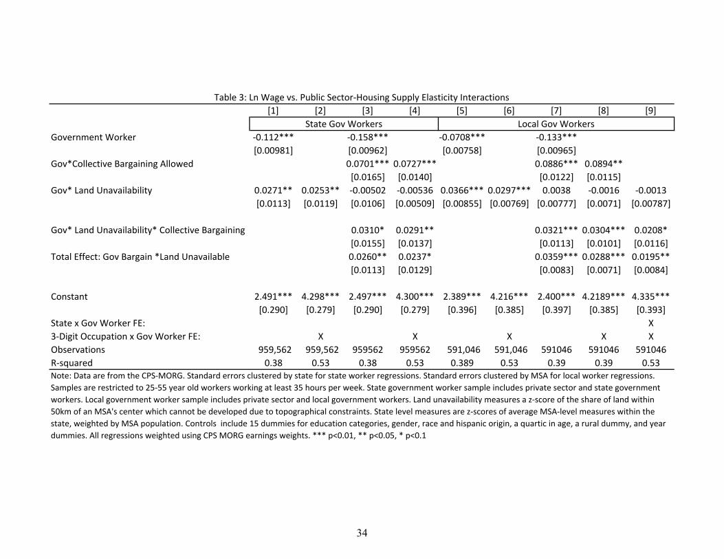
[1] [2] [3] [4] [5] [6] [7] [8] [9]
Government Worker ‐0.112*** ‐0.158*** ‐0.0708*** ‐0.133***
[0.00981] [0.00962] [0.00758] [0.00965]
Gov*Collective Bargaining Allowed 0.0701*** 0.0727*** 0.0886*** 0.0894**
[0.0165] [0.0140] [0.0122] [0.0115]
Gov* Land Unavailability 0.0271** 0.0253** ‐0.00502 ‐0.00536 0.0366*** 0.0297*** 0.0038 ‐0.0016 ‐0.0013
[0.0113] [0.0119] [0.0106] [0.00509] [0.00855] [0.00769] [0.00777] [0.0071] [0.00787]
Gov* Land Unavailability* Collective Bargaining 0.0310* 0.0291** 0.0321*** 0.0304*** 0.0208*
[0.0155] [0.0137] [0.0113] [0.0101] [0.0116]
Total Effect: Gov Bargain *Land Unavailable 0.0260** 0.0237* 0.0359*** 0.0288*** 0.0195**
[0.0113] [0.0129] [0.0083] [0.0071] [0.0084]
Constant 2.491*** 4.298*** 2.497*** 4.300*** 2.389*** 4.216*** 2.400*** 4.2189*** 4.335***
[0.290] [0.279] [0.290] [0.279] [0.396] [0.385] [0.397] [0.385] [0.393]
State x Gov Worker FE: X
3‐Digit Occupation x Gov Worker FE: X X X X X
Observations 959,562 959,562 959562 959562 591,046 591,046 591046 591046 591046
R‐squared 0.38 0.53 0.38 0.53 0.389 0.53 0.39 0.39 0.53
Table 3: Ln Wage vs. Public Sector‐Housing Supply Elasticity Interactions
Note: Data are from the CPS‐MORG. Standard errors clustered by state for state worker regressions. Standard errors clustered by MSA for local worker regressions.
Samples are restricted to 25‐55 year old workers working at least 35 hours per week. State government worker sample includes private sector and state government
workers. Local government worker sample includes private sector and local government workers. Land unavailability measures a z‐score of the share of land within
50km of an MSA's center which cannot be developed due to topographical constraints. State level measures are z‐scores of average MSA‐level measures within the
state, weighted by MSA population. Controls include 15 dummies for education categories, gender, race and hispanic origin, a quartic in age, a rural dummy, and year
dummies. All regressions weighted using CPS MORG earnings weights. *** p<0.01, ** p<0.05, * p<0.1
State Gov Workers Local Gov Workers
34

[1] [2] [3] [4] [5] [6]
Government Worker ‐0.196*** 0.0153 0.0215
[0.0140] [0.0221] [0.0287]
Gov*Collective Bargaining Allowed 0.0921*** 0.151*** 0.174***
[0.0165] [0.0258] [0.0328]
Gov* Land Unavailability 0.0112 0.0138 0.018 0.0148 ‐0.0154 ‐0.0036
[0.0107] [0.0121] [0.0158] [0.0162] [0.0183] [0.0153]
Gov* Land Unavailability* Collective
Bargaining 0.00117 ‐0.0187 0.0338 ‐0.00863 0.0780*** 0.0214
[0.0151] [0.0162] [0.0210] [0.0202] [0.0238] [0.0210]
Total Effect: Gov Bargain *Land
Unavailable 0.0124 ‐0.005 0.0518*** 0.0062 0.0626*** 0.0178
[0.0109] [0.0180] [0.0137] [0.0122] [0.0153] [0.0144]
Constant 2.398*** 2.409*** 2.528*** 2.524*** 2.471*** 2.480***
[0.420] [0.419] [0.422] [0.422] [0.417] [0.419]
State x Gov Worker FE: X X X
Observations 552,890 552,890 538,867 538,867 536,833 536,833
R‐squared 0.39 0.391 0.392 0.392 0.392 0.392
Teachers Police Fire
Note: Standard errors clustered by state. Samples are restricted to 25‐55 year old workers working at least 35 hours per
week. Teachers sample includes all private sector workers and local government workers with teaching occupations.
Police sample includes all private sector and local government police. Fire sample includes all private sector and local
government firefighters. Land unavailability measures a z‐score of the share of land within 50km of an MSA's center which
cannot be developed due to topographical constraints. State level measures are z‐scores of average MSA‐level measures
within the state, weighted by MSA population. Controls include 15 dummies for education categories, gender, race and
hispanic origin, a quartic in age, a rural dummy, and year dummies. All regressions weighted using CPS MORG earnings
weights. *** p<0.01, ** p<0.05, * p<0.1
Table 4: Ln Wage vs. Public Sector‐Housing Supply Elasticity Interactions: Teachers, Police, and Fire
35
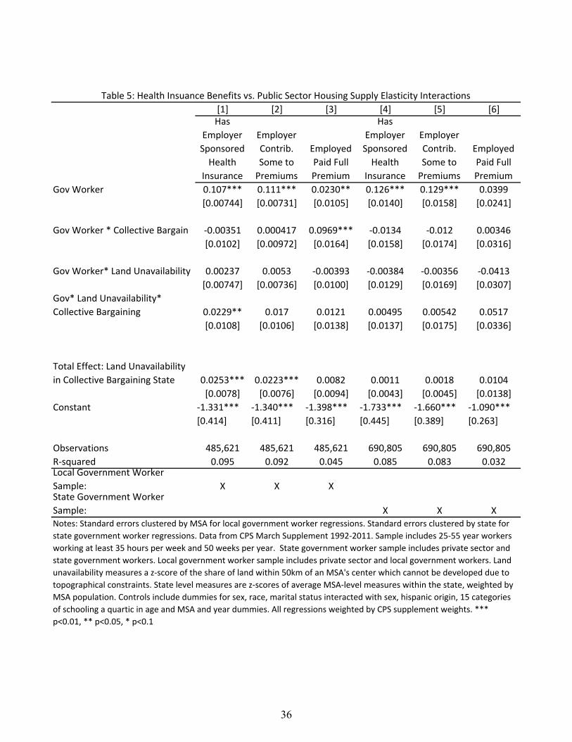
[1] [2] [3] [4] [5] [6]Has
Employer
Sponsored
Health
Insurance
Employer
Contrib.
Some to
Premiums
Employed
Paid Full
Premium
Has
Employer
Sponsored
Health
Insurance
Employer
Contrib.
Some to
Premiums
Employed
Paid Full
Premium
Gov Worker 0.107*** 0.111*** 0.0230** 0.126*** 0.129*** 0.0399
[0.00744] [0.00731] [0.0105] [0.0140] [0.0158] [0.0241]
Gov Worker * Collective Bargain ‐0.00351 0.000417 0.0969*** ‐0.0134 ‐0.012 0.00346
[0.0102] [0.00972] [0.0164] [0.0158] [0.0174] [0.0316]
Gov Worker* Land Unavailability 0.00237 0.0053 ‐0.00393 ‐0.00384 ‐0.00356 ‐0.0413
[0.00747] [0.00736] [0.0100] [0.0129] [0.0169] [0.0307]
Gov* Land Unavailability*
Collective Bargaining 0.0229** 0.017 0.0121 0.00495 0.00542 0.0517
[0.0108] [0.0106] [0.0138] [0.0137] [0.0175] [0.0336]
Total Effect: Land Unavailability
in Collective Bargaining State 0.0253*** 0.0223*** 0.0082 0.0011 0.0018 0.0104
[0.0078] [0.0076] [0.0094] [0.0043] [0.0045] [0.0138]
Constant ‐1.331*** ‐1.340*** ‐1.398*** ‐1.733*** ‐1.660*** ‐1.090***
[0.414] [0.411] [0.316] [0.445] [0.389] [0.263]
Observations 485,621 485,621 485,621 690,805 690,805 690,805
R‐squared 0.095 0.092 0.045 0.085 0.083 0.032Local Government Worker
Sample: X X XState Government Worker
Sample: X X X
Table 5: Health Insuance Benefits vs. Public Sector Housing Supply Elasticity Interactions
Notes: Standard errors clustered by MSA for local government worker regressions. Standard errors clustered by state for
state government worker regressions. Data from CPS March Supplement 1992‐2011. Sample includes 25‐55 year workers
working at least 35 hours per week and 50 weeks per year. State government worker sample includes private sector and
state government workers. Local government worker sample includes private sector and local government workers. Land
unavailability measures a z‐score of the share of land within 50km of an MSA's center which cannot be developed due to
topographical constraints. State level measures are z‐scores of average MSA‐level measures within the state, weighted by
MSA population. Controls include dummies for sex, race, marital status interacted with sex, hispanic origin, 15 categories
of schooling a quartic in age and MSA and year dummies. All regressions weighted by CPS supplement weights. ***
p<0.01, ** p<0.05, * p<0.1
36

[1] [2] [3] [4]
Land Unavailability 0.0493 0.117** 0.141*** 0.256***
[0.0355] [0.0488] [0.0373] [0.0524]
Collective Bargaining ‐0.0468*
[0.0263]
Bargain*Unavailability ‐0.0828 ‐0.228***
[0.0719] [0.0823]
Constant 0.265*** 0.300*** 0.475*** 0.465***
[0.0126] [0.0215] [0.0418] [0.0421]
Total Effect: Land Unavailability w/ Collective
Bargaining 0.034 0.0274
[0.0528] [0.0634]
State FE: X X
Observations 236 236 176 176
R‐squared 0.069 0.127 0.546 0.572
Table 6: Public Corruption Convictions within Federal District Court per Capita vs Housing
Supply Elasticity & Collective Bargaining Laws
Note: Standard errors clustered by MSA. Corruption data comes from annual reports of the Public
Integrity Section of the US Department of Justice. Data measures total number of annual corruption
convictions within relavant federal district. Federal districts have been linked to MSAs by geogrpahy.
MSA spanning multiple states are dropped from the analysis. States with only a single district court
for the entire state are dropped from the state fixed effects analysis. Land unavailability measure is
multiplied by the population share covered by the federal district court contained within the MSA.
Population share is also included as a control. *** p<0.01, ** p<0.05, * p<0.1
37

[1] [2] [3] [4] [5] [6] [7] [8] [9] [10]
Land Unavailability ‐0.216** ‐0.319* ‐0.228** ‐0.174 0.0169** 0.0286** 0.0190** 0.0125 0.0504* 0.0765*
[0.0913] [0.165] [0.0984] [0.156] [0.00746] [0.0134] [0.00762] [0.0133] [0.0263] [0.0447]
Bargain*Unavailability 0.141 ‐0.0722 ‐0.0161 0.00858 ‐0.0360
[0.189] [0.197] [0.0154] [0.0161] [0.0549]
Constant 14.90*** 14.86*** 14.94*** 14.96*** 0.0140*** 0.0187** 0.00787* 0.00536 0.172** 0.183**
[0.0621] [0.0934] [0.0577] [0.0741] [0.00495] [0.00760] [0.00459] [0.00610] [0.0778] [0.0774]
Observations 5,963 5,963 5,443 5,443 5,963 5,963 5,443 5,443 5,963 5,963
R‐squared 0.176 0.176 0.178 0.178 0.162 0.162 0.170 0.170 0.305 0.305
Notes: Outcome data come from the ICMA Form of Government Survey from 1996‐2002. Max number of terms for chief officer and counsil
members is coded to 15 for areas with no term limits. Counsil member term limits were ask only of city governments, not county. Chief
office has a term limit is a dummy variable for whether the chief officer has a cap on the number of terms s/he can serve. The Counsil
member term cap variable is defined similarly. The Voter Legislation Power Index is a score from 0 to 4, where 1 point is receieved for each
voter legislation power allowed in the area: initiative, referendum, recall, and protest referendum. See text for detailed definitions of each
of these. All regressions included state fixed effects. Standard errors are clustered by MSA. *** p<0.01, ** p<0.05, * p<0.1
Table 7: Voter Empowerment vs Land UnavailabilityMax Number of
Terms for Chief
Officer
Max Number of
Terms for Counsil
Members
Chief Officer Has A
Term Cap
Counsil Members
Have Term Caps
Voter Legislation
Power Index
38
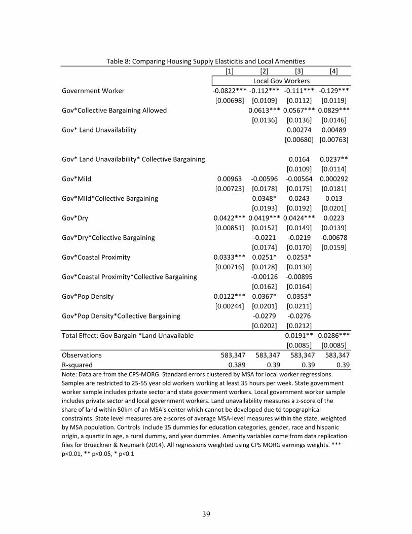
[1] [2] [3] [4]
Government Worker ‐0.0822*** ‐0.112*** ‐0.111*** ‐0.129***
[0.00698] [0.0109] [0.0112] [0.0119]
Gov*Collective Bargaining Allowed 0.0613*** 0.0567*** 0.0829***
[0.0136] [0.0136] [0.0146]
Gov* Land Unavailability 0.00274 0.00489
[0.00680] [0.00763]
Gov* Land Unavailability* Collective Bargaining 0.0164 0.0237**
[0.0109] [0.0114]
Gov*Mild 0.00963 ‐0.00596 ‐0.00564 0.000292
[0.00723] [0.0178] [0.0175] [0.0181]
Gov*Mild*Collective Bargaining 0.0348* 0.0243 0.013
[0.0193] [0.0192] [0.0201]
Gov*Dry 0.0422*** 0.0419*** 0.0424*** 0.0223
[0.00851] [0.0152] [0.0149] [0.0139]
Gov*Dry*Collective Bargaining ‐0.0221 ‐0.0219 ‐0.00678
[0.0174] [0.0170] [0.0159]
Gov*Coastal Proximity 0.0333*** 0.0251* 0.0253*
[0.00716] [0.0128] [0.0130]
Gov*Coastal Proximity*Collective Bargaining ‐0.00126 ‐0.00895
[0.0162] [0.0164]
Gov*Pop Density 0.0122*** 0.0367* 0.0353*
[0.00244] [0.0201] [0.0211]
Gov*Pop Density*Collective Bargaining ‐0.0279 ‐0.0276
[0.0202] [0.0212]
Total Effect: Gov Bargain *Land Unavailable 0.0191** 0.0286***
[0.0085] [0.0085]
Observations 583,347 583,347 583,347 583,347
R‐squared 0.389 0.39 0.39 0.39
Local Gov Workers
Table 8: Comparing Housing Supply Elasticitis and Local Amenities
Note: Data are from the CPS‐MORG. Standard errors clustered by MSA for local worker regressions.
Samples are restricted to 25‐55 year old workers working at least 35 hours per week. State government
worker sample includes private sector and state government workers. Local government worker sample
includes private sector and local government workers. Land unavailability measures a z‐score of the
share of land within 50km of an MSA's center which cannot be developed due to topographical
constraints. State level measures are z‐scores of average MSA‐level measures within the state, weighted
by MSA population. Controls include 15 dummies for education categories, gender, race and hispanic
origin, a quartic in age, a rural dummy, and year dummies. Amenity variables come from data replication
files for Brueckner & Neumark (2014). All regressions weighted using CPS MORG earnings weights. ***
p<0.01, ** p<0.05, * p<0.1
39

[1] [2] [3] [4] [5] [6] [7] [8]
Growing
Pop
Shrinking
Pop
Growing
Pop
Shrinking
Pop
Growing
Pop
Shrinking
Pop
Growing
Pop
Shrinking
Pop
Gov Worker ‐0.133*** ‐0.157*** ‐0.198*** ‐0.137* 0.0214 ‐0.109 0.0325 ‐0.471**
[0.00984] [0.0276] [0.0145] [0.0759] [0.0222] [0.111] [0.0305] [0.186]
Gov Worker * Collective Bargain 0.0851*** 0.128*** 0.0822*** 0.130* 0.146*** 0.243** 0.168*** 0.612***
[0.0129] [0.0289] [0.0170] [0.0764] [0.0265] [0.114] [0.0348] [0.186]
Gov* Land Unavailability* Collective
Bargaining 0.0349*** ‐0.00278 0.00381 0.000688 0.0286 ‐0.000447 0.0566* ‐0.0516
[0.0119] [0.0188] [0.0162] [0.0397] [0.0220] [0.0650] [0.0320] [0.0891]
Gov Worker* Land Unavailability 0.00419 0.0102 0.0118 ‐0.00998 0.0258 ‐0.0264 0.00712 0.0923
[0.00823] [0.0140] [0.0118] [0.0330] [0.0169] [0.0468] [0.0279] [0.0815]
Total Effect: Land Unavailability in
Collective Bargaining State 0.0391*** 0.0074 0.0156 ‐0.0093 0.0544*** ‐0.0269 0.0637*** 0.0407
[0.0086] [0.0126] [0.0114] [0.0219] [0.0140] [0.0441] [0.0158] [0.0286]
Constant 2.394*** 2.272** 2.384*** 2.362** 2.521*** 2.291* 2.467*** 2.206*
[0.418] [1.092] [0.441] [1.092] [0.444] [1.197] [0.440] [1.167]
Observations 542,701 46,863 507,746 43,744 495,093 42,416 493,207 42,277
R‐squared 0.391 0.370 0.392 0.371 0.394 0.369 0.394 0.369Note: Standard errors clustered by MSA. Samples are restricted to 25‐55 year old workers working at least 35 hours per week. Teachers sample
includes all private sector workers and local government workers with teaching occupations. Police sample includes all private sector and local
government police. Fire sample includes all private sector and local government firefighters. Land unavailability measures a z‐score of the share
of land within 50km of an MSA's center which cannot be developed due to topographical constraints. Controls include 15 dummies for
education categories, gender, race and hispanic origin, a quartic in age, a rural dummy, and year dummies. All regressions weighted using CPS
MORG earnings weights. *** p<0.01, ** p<0.05, * p<0.1
Table 9: Ln Wage vs. Public Sector‐Housing Supply Elasticity Interactions, Growing and Shrinking MSAs
All Local Workers Teachers Police Fire
40

[1] [2] [3] [4] [5] [6]
State Gov
Workers
State Gov
Workers
Government Worker 0.184*** 0.190*** 0.0846*** 0.0804***
[0.0116] [0.0225] [0.00839] [0.0101]
Gov*Collective Bargaining Allowed ‐0.0502*** ‐0.0433* ‐0.0121 ‐0.00557
[0.0140] [0.0254] [0.0120] [0.0125]
Gov*Land Unavailable 0.00502 0.0102 0.0122 ‐0.00181 0.00448 ‐0.00851
[0.00814] [0.00937] [0.0219] [0.0134] [0.00656] [0.00904]
Gov*Land Unavailable*Bargain
Allowed ‐0.0347** ‐0.0233* ‐0.0345 0.0138 0.00597 0.0111
[0.0158] [0.0137] [0.0264] [0.0195] [0.0108] [0.0104]
Total Effect: Gov Bargain *Land
Unavailable ‐0.0297** ‐0.0131 ‐0.0223 0.0120 0.0104 0.0026
[0.0136] [0.0100] [0.0147] [0.0142] [0.0086] [0.0051]
Constant 2.712*** 2.427*** 2.305*** ‐1.412*** ‐1.347*** ‐1.729***
[0.413] [0.412] [0.292] [0.452] [0.412] [0.408]
State FE X X
MSA FE X X X X
State x Gov Worker FE: X X
Observations 564,524 554,022 935,421 463869 459,650 676,858
R‐squared 0.389 0.394 0.383 0.089 0.088 0.079Note:Standard errors clustered by MSA for state worker regressions. Standard errors clustered by MSA for federal
government worker regressions using cross MSA variation in land unavailability. Standard errors clustered by state for
federal government worker regressions using cross state variation in land unavailability. Weekly wage data from 1995‐
2011 CPS MORG. Wage data is restricted to 25‐55 year old workers working at least 35 hours per week. Health
insurnace data are from 1991‐2011 March CPS Supplement. State government worker sample includes private sector
and state government workers. Federal government work sample includes private sector and federal government
workers. Land unavailability measures a z‐score of the share of land within 50km of an MSA's center which cannot be
developed due to topological constraints. State level measures are z‐scores of average MSA‐level measures within the
state, weighted by MSA population. Controls include 15 dummies for education categories, gender, race, Hispanic
origin, a quartic in age, a rural dummy, and year dummies. All regressions weighted by appropriate CPS weights. ***
p<0.01, ** p<0.05, * p<0.1
Table 10: State & Federal Government Workers Falsification Tests
Federal Gov Workers
Ln Wage
Employer Contributed Some to
Health Insurance Premiums
Federal Gov Workers
41

[1] [2] [3] [4] [5] [6] [7]
State Gov Local Gov
Government Worker 1.938*** 1.265*** 1.980*** 1.961***
[0.0637] [0.0547] [0.0950] [0.126]
Gov*Collective Bargaining Allowed ‐0.347*** ‐0.06 0.193*** 0.146*** 0.0244 ‐0.135
[0.121] [0.0526] [0.0727] [0.0402] [0.143] [0.153]
Gov* Land Unavailability ‐0.0168 ‐0.00723 0.0156 ‐0.0101 0.0499 0.141 0.0661
[0.0559] [0.0233] [0.0493] [0.0258] [0.0411] [0.124] [0.119]
Gov* Land Unavailability* Collective Bargaining 0.0178 0.0777 ‐0.0622 0.0616 ‐0.0497 ‐0.0256 0.235
[0.0987] [0.0513] [0.0705] [0.0413] [0.0498] [0.196] [0.150]
Total Effect: Gov Bargain *Land Unavailable 0.0009 0.0705 ‐0.0466 0.0515 0.0002 0.1156 0.3016***
[0.0813] [0.0473] [0.0506] [0.0335] [0.0286] [0.1501] [0.0908]
Constant 13.86*** 4.057*** 13.89*** 14.56*** 14.56*** 42.17*** 42.85***
[0.187] [1.208] [0.173] [0.130] [0.130] [0.356] [0.394]
State x Gov Worker FE: X
3‐Digit Occupation x Gov Worker FE: X X X
Observations 959562 959562 591046 591046 591046 959,562 591,046
R‐squared 0.18 0.50 0.19 0.50 0.51 0.03 0.035Note: Data are from the CPS‐MORG. Standard errors clustered by state for state worker regressions. Standard errors clustered by MSA for
local worker regressions. Lefthand side variable is years of schooling completed by worker in columns 1‐5. Lefthand side variable is worker age
in columns 6 and 7. Samples are restricted to 25‐55 year old workers working at least 35 hours per week. Controls include gender, race and
hispanic origin, a quartic in age, schooling, a rural dummy, and year dummies. Age is removed as a control in the age regressions and
schooling is removed as a control in the schooling regressions. All regressions weighted using CPS MORG earnings weights. *** p<0.01, **
p<0.05, * p<0.1
Worker Age
Table 11: Worker Sorting into Public Sector Jobs & Housing Supply Elasticity
State Gov Workers Local Gov Workers
Years of Schooling
42

Figure 1: State Goverment-Private Sector Wages Gaps vs. State Land Unavailability & Collective Bargaining Laws
ND
VA
NC
SC
GAKY
TN
AL
MS
AR
LA
OK
TXID
CO
UT
NV
ME
NH
VT
MA
RI CTNY
NJPA
OH
IN
IL
MI
WIMN
IA
MO
SDNE
KS
DEMD
WV
FLMT
NMAZ
WAOR
CA
β =0.0050 (0.011)
β =0.0260 (0.0113)
.2.1
5.1
.05
0Pu
blic
Priv
ate
Wag
e G
ap
1 0 1 2 3State Average Land Unavai labil i ty in MSAs: ZScore
No State Worker Unions Allows State Worker Unions
Notes: Data from CPS-MORG. State wage gaps calculated after residualizing wages against15 dummies for education categories, gender, race, hispanic origin, a quartic in age, a rural
dummy, and year dummies. Regression weighted using CPS earnings weights.
43
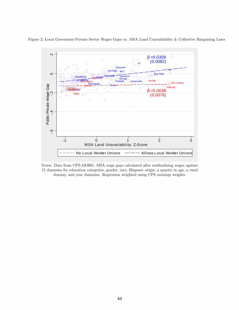
Figure 2: Local Goverment-Private Sector Wages Gaps vs. MSA Land Unavailability & Collective Bargaining Laws
Boston
ChicagoClevelandDetroit
Jacksonville
KansasCity
LasVegas
LA
Minneapolis
NYC
PhiladelphiaPhoeniz
Pittsburgh
Portland
Riverside
StLouis
San Diego
SF
Atlanta
Baltimore
Charlotte
Dallas
DenverHouston
New OrleansNorfolk
SaltLake
Washington
β =0.0038 (0.0078)
β =0.0359 (0.0082)
.6.4
.20
.2Pu
blic
Priv
ate
Wag
e G
ap
1 0 1 2 3MSA Land Unavai labil i ty: ZScore
No Local Worker Unions Allows Local Worker Unions
Notes: Data from CPS-MORG. MSA wage gaps calculated after residualizing wages against15 dummies for education categories, gender, race, Hispanic origin, a quartic in age, a rural
dummy, and year dummies. Regression weighted using CPS earnings weights.
44

A Government Taxation under Income and Property Taxes
In all the cases below I do not model the public sector labor market. This allows the analysis to
focus on the role of the tax instrument in rent extraction.
A.1 Income Tax
A.1.1 Government
The local government of city j charges an income tax τ j to workers who choose to reside within
the city. The local government also produces government services, which cost sj for each worker in
the city. Nj measure the population of city j. The local rent seeking government maximizes:
maxτ j ,sj
τ jwjNj − sjNj
A.1.2 Workers
All workers are homogeneous. Workers living in city j inelastically supply one unit of labor, and
earn wage wj . Each worker must rent a house to live in the city at rental rate rj and pay the local
income tax τ j . Workers value the local amenities as measure by Aj .The desirability of government
services sj is represented by g (sj) . Thus, workers’utility from living in city j is:
Uj = wj (1− τ j)− rj +Aj + g (sj) .
Workers maximize their utility by living in the city which they find the most desirable.
A.1.3 Firms
All firms are homogenous and produce a tradeable output Y.Cities exogenously differ in their
productivity as measured by θj . Local government services impact firms productivity, as measured
by b(sj). The production function is:
Yj = θjNj + b(sj)Nj .
I
I assume a completely elastic labor demand curve to focus on the role of housing supply elasticity
in setting tax rates.
The labor market is perfectly competitive, so wages equal the marginal product of labor:
wj = θj + b(sj).
45

A.1.4 Housing
The housing market is identical to the setting described in the main text in Section 3.4. The
housing supply curve is:
rj = aj + γj log (Nj) ,
γj = γxhousej
where xhousej is a vector of city characteristics which impact the elasticity of housing supply.
A.1.5 Equilibrium in Labor and Housing
Since all workers are identical, all cities with positive population must offer equal utility to workers.
In equilibrium, all workers must be indifferent between all cities. Thus:
Uj = wj (1− τ j)− rj +Aj + g (sj) = U .
Plugging in labor demand and housing supply gives:
(θj + b(sj)) (1− τ j)− aj − γj logNj +Aj + g (sj) = U . (11)
Equation (11) determines the equilibrium distribution of workers across cities.
A.1.6 Government Tax Competition
The government maximizes:
maxsj ,τ j
τ jwjNj − sjNj .
The first order conditions are:
0 = wjτ j∂Nj
∂sj+ τ jNj
∂wj∂Nj
∂Nj
∂sj−Nj − sj
∂Nj
∂sj(12)
0 = τ j
(∂wj∂Nj
∂Nj
∂τ jNj + wj
∂Nj
∂τ j
)+ wjNj − sj
∂Nj
∂τ j.
Differentiating equation (11) to solve for ∂Nj∂sj
and ∂Nj∂τ jgives:
∂Nj
∂sj= Nj
(1− τ j) b′ (sj) + g′ (sj)
γj> 0
∂Nj
∂τ j= −Nj
(θj + b(sj))
γj< 0. (13)
Population increases with government services and decreases in taxes. Plugging these into (12)
and combining the first order conditions shows that government services are provided such that the
46
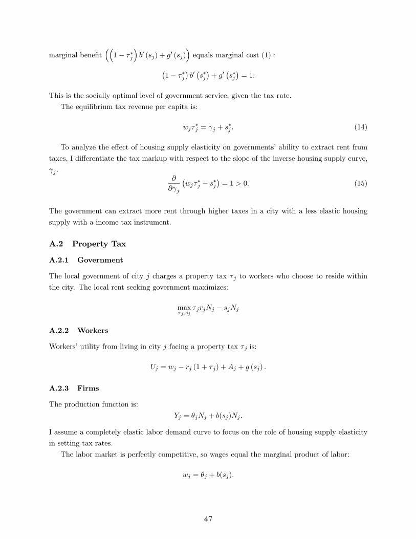
marginal benefit((
1− τ∗j)b′ (sj) + g′ (sj)
)equals marginal cost (1) :
(1− τ∗j
)b′(s∗j)
+ g′(s∗j)
= 1.
This is the socially optimal level of government service, given the tax rate.
The equilibrium tax revenue per capita is:
wjτ∗j = γj + s∗j . (14)
To analyze the effect of housing supply elasticity on governments’ability to extract rent from
taxes, I differentiate the tax markup with respect to the slope of the inverse housing supply curve,
γj .∂
∂γj
(wjτ
∗j − s∗j
)= 1 > 0. (15)
The government can extract more rent through higher taxes in a city with a less elastic housing
supply with a income tax instrument.
A.2 Property Tax
A.2.1 Government
The local government of city j charges a property tax τ j to workers who choose to reside within
the city. The local rent seeking government maximizes:
maxτ j ,sj
τ jrjNj − sjNj
A.2.2 Workers
Workers’utility from living in city j facing a property tax τ j is:
Uj = wj − rj (1 + τ j) +Aj + g (sj) .
A.2.3 Firms
The production function is:
Yj = θjNj + b(sj)Nj .
I assume a completely elastic labor demand curve to focus on the role of housing supply elasticity
in setting tax rates.
The labor market is perfectly competitive, so wages equal the marginal product of labor:
wj = θj + b(sj).
47

A.2.4 Housing
The housing market is identical to the setting described in the main text in Section 3.4. The
housing supply curve is:
rj = aj + γj log (Nj) ,
γj = γxhousej
where xhousej is a vector of city characteristics which impact the elasticity of housing supply.
A.2.5 Equilibrium in Labor and Housing
Since all workers are identical, all cities with positive population must offer equal utility to workers.
In equilibrium, all workers must be indifferent between all cities. Thus:
Uj = wj − rj (1 + τ j) +Aj + g (sj) = U .
Plugging in labor demand and housing supply gives:
(θj + b(sj))−(aj + γj logNj
)(1 + τ j) +Aj + g (sj) = U . (16a)
Equation (16a) determines the equilibrium distribution of workers across cities.
A.2.6 Government Tax Competition
The government maximizes:
maxsj ,τ j
τ jrjNj − sjNj .
The first order conditions are:
0 = rjτ j∂Nj
∂sj+ τ jNj
∂rj∂Nj
∂Nj
∂sj−Nj − sj
∂Nj
∂sj(17)
0 = τ j
(∂rj∂Nj
∂Nj
∂τ jNj + rj
∂Nj
∂τ j
)+ rjNj − sj
∂Nj
∂τ j. (18)
Differentiating equation (16a) to solve for ∂Nj∂sj
and ∂Nj∂τ jgives:
∂Nj
∂sj= Nj
b′ (sj) + g′ (sj)
γj (1 + τ j)> 0
∂Nj
∂τ j= −Nj
rjγj (1 + τ j)
< 0. (19)
Combining the first order conditions shows that government services are provided such that the
marginal benefit (b′ (sj) + g′ (sj)) equals marginal cost (1) , which is the same finding for an income
48

tax and head tax:
b′(s∗j)
+ g′(s∗j)
= 1.
Plugging (19) into (18) and rearranging shows the equilibrium tax revenue per capita is:
rjτ∗j = γj + s∗j . (20)
Differentiating the tax markup with respect to the slope of the inverse housing supply curve, γj .
∂
∂γj
(wjτ
∗j − s∗j
)= 1 > 0. (21)
The government can extract more rent through higher taxes in a city with a less elastic housing
supply using a property tax instrument. In the case of a property tax, as opposed to a head tax,
there are four mechanisms through which a tax rate change impacts government revenue. To break
these down, I rewrite the tax rate first order condition:
0 = τ jrj∂Nj
∂τ j︸ ︷︷ ︸Decline in revenue due
to population decrease
+ τ j∂rj∂Nj
∂Nj
∂τ jNj︸ ︷︷ ︸
Decline in revenue
due to rent decrease
+ rjNj︸︷︷︸Additional tax revenue
from each resident
− sj∂Nj
∂τ j︸ ︷︷ ︸Government services
cost savings
(22)
First, the amount of out-migration driven by a tax hike is influenced by the local housing
supply elasticity. This is the first term of equation (22) . Second, the out-migration lowers rents
and directly impacts tax revenues since the tax revenue is a percentage of housing rents. This is
the second term of equation (22) . However, the housing supply elasticity will not impact the size
of the rental rate decrease in response to a tax hike. To see this, recall the equilibrium condition,
equation (16a) . For workers to derive utility U from this local area, the utility impact of a tax
increase must be perfectly offset by a rent decrease.26 Thus, the equilibrium rental rate response
to a given tax increase does not depend on the local housing supply elasticity. Indeed, the housing
supply elasticity determines the migration response required to change housing rents in order to
offset the utility impact of the tax increase. Thus, a more inelastic housing supply decreases the
elasticity of government revenue with respect to the tax rate, giving the government more market
power when using a property tax instrument.
The third and forth terms of equation (22) show a tax increase raises government revenues from
each household and lowers the cost of government services due to out-migration. These channels
also appear in the case of a head tax instrument.
26Since I have assumed a perfectly elastic labor demand curve, the rental rate response to a tax increase wouldbe the same in any city. However, if labor demand was not perfectly elastic, then the rental rate response to atax increase could differ with housing supply elasticity, since housing supply elasticity would influence the relativeincidence of the tax rate on wages versus rents.
49
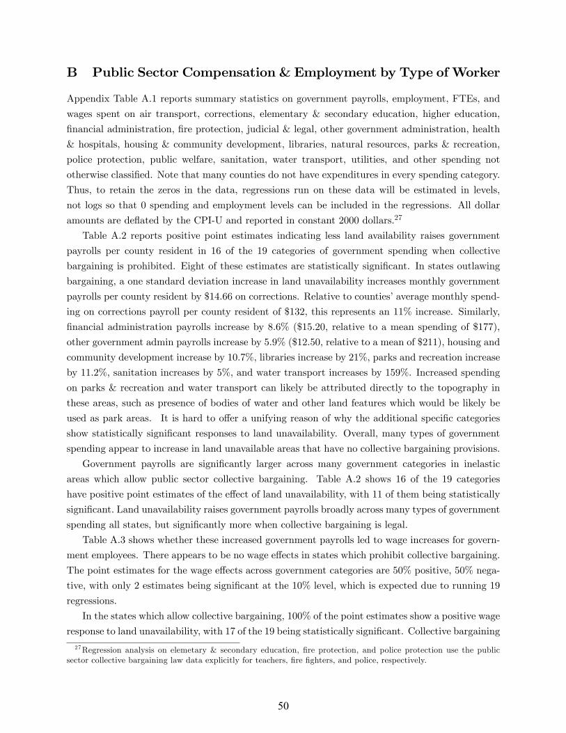
B Public Sector Compensation & Employment by Type of Worker
Appendix Table A.1 reports summary statistics on government payrolls, employment, FTEs, and
wages spent on air transport, corrections, elementary & secondary education, higher education,
financial administration, fire protection, judicial & legal, other government administration, health
& hospitals, housing & community development, libraries, natural resources, parks & recreation,
police protection, public welfare, sanitation, water transport, utilities, and other spending not
otherwise classified. Note that many counties do not have expenditures in every spending category.
Thus, to retain the zeros in the data, regressions run on these data will be estimated in levels,
not logs so that 0 spending and employment levels can be included in the regressions. All dollar
amounts are deflated by the CPI-U and reported in constant 2000 dollars.27
Table A.2 reports positive point estimates indicating less land availability raises government
payrolls per county resident in 16 of the 19 categories of government spending when collective
bargaining is prohibited. Eight of these estimates are statistically significant. In states outlawing
bargaining, a one standard deviation increase in land unavailability increases monthly government
payrolls per county resident by $14.66 on corrections. Relative to counties’average monthly spend-
ing on corrections payroll per county resident of $132, this represents an 11% increase. Similarly,
financial administration payrolls increase by 8.6% ($15.20, relative to a mean spending of $177),
other government admin payrolls increase by 5.9% ($12.50, relative to a mean of $211), housing and
community development increase by 10.7%, libraries increase by 21%, parks and recreation increase
by 11.2%, sanitation increases by 5%, and water transport increases by 159%. Increased spending
on parks & recreation and water transport can likely be attributed directly to the topography in
these areas, such as presence of bodies of water and other land features which would be likely be
used as park areas. It is hard to offer a unifying reason of why the additional specific categories
show statistically significant responses to land unavailability. Overall, many types of government
spending appear to increase in land unavailable areas that have no collective bargaining provisions.
Government payrolls are significantly larger across many government categories in inelastic
areas which allow public sector collective bargaining. Table A.2 shows 16 of the 19 categories
have positive point estimates of the effect of land unavailability, with 11 of them being statistically
significant. Land unavailability raises government payrolls broadly across many types of government
spending all states, but significantly more when collective bargaining is legal.
Table A.3 shows whether these increased government payrolls led to wage increases for govern-
ment employees. There appears to be no wage effects in states which prohibit collective bargaining.
The point estimates for the wage effects across government categories are 50% positive, 50% nega-
tive, with only 2 estimates being significant at the 10% level, which is expected due to running 19
regressions.
In the states which allow collective bargaining, 100% of the point estimates show a positive wage
response to land unavailability, with 17 of the 19 being statistically significant. Collective bargaining
27Regression analysis on elemetary & secondary education, fire protection, and police protection use the publicsector collective bargaining law data explicitly for teachers, fire fighters, and police, respectively.
50

seems to channel these extra payroll dollars into higher government wages across essentially all types
of government spending.
Table A.4 shows the effects of land unavailability on government FTEs per county resident.
In states which prohibit collective bargaining, the categories which showed a significant positive
government payroll response to land unavailability also show a statistically significant FTE per
county resident response as well. These additional dollars all appear to go to a larger government
workforce when collective bargaining is prohibited.
Within states which allow collective bargaining, government FTEs appear to statistically sig-
nificantly rise in air transport, higher education, and parks & recreation. FTEs fall in elementary
& secondary education, and libraries. The other point estimates are a mix of both positive and
negative effects. There does not appear to be a clear increase in FTEs in collective bargaining
states. Table A.5 looks at government employment counts per county resident and shows very
similar results as those for the government FTEs.
51
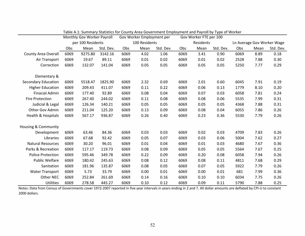
Obs Mean Std. Dev. Obs Mean Std. Dev. Obs Mean Std. Dev. Obs Mean Std. Dev.
County Area Overall 6069 9275.80 3142.16 6069 4.02 1.06 6069 3.41 0.90 6069 8.89 0.18
Air Transport 6069 19.67 89.11 6069 0.01 0.02 6069 0.01 0.02 2528 7.88 0.30
Correction 6069 132.07 141.04 6069 0.05 0.05 6069 0.05 0.05 5250 7.77 0.29
Elementary &
Secondary Education 6069 5518.47 1825.90 6069 2.32 0.69 6069 2.01 0.60 6045 7.91 0.19
Higher Education 6069 209.43 411.07 6069 0.11 0.22 6069 0.06 0.13 1779 8.10 0.20
Finacial Admin 6069 177.40 92.89 6069 0.08 0.04 6069 0.07 0.03 6058 7.81 0.24
Fire Protection 6069 267.40 244.02 6069 0.11 0.08 6069 0.08 0.06 5535 7.99 0.31
Judicial & Legal 6069 126.34 140.21 6069 0.05 0.05 6069 0.05 0.05 4368 7.88 0.31
Other Gov Admin 6069 211.04 125.20 6069 0.13 0.09 6069 0.08 0.04 6055 7.86 0.26
Health & Hospitals 6069 567.17 936.87 6069 0.26 0.40 6069 0.23 0.36 5530 7.79 0.26
Housing & Community
Development 6069 63.46 84.36 6069 0.03 0.03 6069 0.02 0.03 4709 7.83 0.26
Libraries 6069 67.68 92.42 6069 0.05 0.07 6069 0.03 0.06 5004 7.62 0.27
Natural Resources 6069 30.20 96.01 6069 0.01 0.04 6069 0.01 0.03 4680 7.67 0.36
Parks & Recreation 6069 117.17 119.73 6069 0.08 0.09 6069 0.05 0.05 5564 7.67 0.25
Police Protection 6069 595.46 349.78 6069 0.22 0.09 6069 0.20 0.08 6058 7.94 0.26
Public Welfare 6069 180.42 245.63 6069 0.08 0.12 6069 0.08 0.11 4811 7.68 0.29
Sanitation 6069 181.96 135.87 6069 0.08 0.05 6069 0.07 0.05 5922 7.79 0.26
Water Transport 6069 5.73 33.79 6069 0.00 0.01 6069 0.00 0.01 681 7.99 0.36
Other NEC 6069 252.84 261.69 6069 0.14 0.16 6069 0.10 0.10 6034 7.75 0.26
Utilities 6069 278.58 445.27 6069 0.10 0.12 6069 0.09 0.11 5790 7.88 0.25
Gov Worker FTE per 100
Residents Ln Average Gov Worker Wage
Notes: Data from Census of Governments cover 1972‐2007 reported in five year intervals in years ending in 2 and 7. All dollar amounts are deflated by CPI‐U to constant
2000 dollars.
Table A.1: Summary Statistics for County Area Government Employment and Payroll by Type of WorkerMonthly Gov Worker Payroll
per 100 Residents
Gov Worker Employment per
100 Residents
52

[1] [2] [3] [4] [5] [6] [7] [8] [9] [10]
Monthly Gov
Pay/100
Residents Air Transport Correction
Elementary
& Secondary
Education
Higher
Education
Finacial
Admin
Fire
Protection
Judicial &
Legal
Other Gov
Admin
Health &
Hospitals
Land
Unavailability 127.1 ‐1.969 14.66* 113.3 ‐15.49 15.20** 12.27 5.248 12.50* ‐57.27
[165.6] [2.183] [7.920] [123.1] [17.02] [6.849] [20.66] [8.432] [7.050] [50.98]
Collective
Bargainings 1279.1*** 0.659 36.14*** 612.0*** 157.9*** 14.05* 33.07* 49.12*** 61.51*** ‐64.28
[260.0] [4.356] [9.952] [136.9] [28.41] [8.455] [19.47] [9.216] [10.37] [68.30]
Bargain*Unavai
lability 470.0* 10.05** 21.78* ‐111.7 68.93** 14.28* 41.59* 16.1 20.64* 82.16
[254.6] [4.080] [12.22] [141.8] [27.67] [7.817] [23.44] [11.72] [11.95] [69.57]
Constant 7629.4*** 9.870*** 29.24*** 4,838*** 83.21*** 142.1*** 208.1*** ‐24.61*** 226.5*** 484.5***
[161.38] [2.119] [4.769] [114.5] [19.34] [6.198] [12.19] [5.940] [7.924] [49.43]
Observations 6,069 6,069 6,069 6,069 6,069 6,069 6,069 6,069 6,069 6,069
R‐squared 0.16 0.01 0.254 0.107 0.048 0.153 0.065 0.374 0.21 0.007
[11] [12] [13] [14] [15] [16] [17] [18 [19] [20]
Housing &
Community
Develop Libraries
Natural
Resources
Parks &
Recreation
Police
Protection
Public
Welfare Sanitation
Water
Transport Other NEC Utilities
Land
Unavailability 6.791** 14.08** 7.922 13.08* 12.89 15.37 9.014* 9.153** 12.06 8.319
[2.740] [7.037] [5.730] [6.851] [16.08] [16.80] [4.882] [4.554] [11.63] [16.02]
Collective
Bargainings 8.216* 14.66* 11.19** 14.85 93.63*** 124.1*** ‐1.444 ‐1.306 20.56 40.16
[4.338] [7.838] [5.549] [10.41] [29.26] [25.00] [8.403] [3.211] [15.29] [28.46]
Bargain*Unavai
lability 6.999* ‐9.442 2.263 23.89*** 94.63*** 18.85 16.73** ‐2.404 38.59** 35.63
[4.029] [7.862] [5.467] [8.965] [28.93] [22.30] [7.786] [4.309] [15.15] [30.93]
Constant 41.95*** 41.52*** 25.92*** 83.97*** 393.1*** 75.65*** 162.7*** 8.328*** 212.5*** 197.5***
[2.801] [5.014] [4.378] [6.966] [16.03] [11.81] [5.969] [2.712] [10.83] [17.73]
Observations 6,069 6,069 6,069 6,069 6,069 6,069 6,069 6,069 6,069 6,069
R‐squared 0.035 0.06 0.013 0.082 0.178 0.091 0.026 0.045 0.056 0.012
Table A.2: County Area Government Payroll per 100 Residents by Category vs. Housing Supply Elasticity Interactions
Notes: Standard errors clustered by MSA. Data on monthly government payroll per capita is measured in constast 2000 dollars. Counties with zero spending in a given
category are included in regressions. Controls include year dummies. *** p<0.01, ** p<0.05, * p<0.1
53

[1] [2] [3] [4] [5] [6] [7] [8] [9] [10]
Average Gov
Wage Air Transport Correction
Elementary
& Secondary
Education
Higher
Education
Finacial
Admin
Fire
Protection
Judicial &
Legal
Other Gov
Admin
Health &
Hospitals
Land Unavailability ‐0.00476 ‐0.00725 0.00294 ‐0.00339 0.0196* 0.00404 ‐0.0125 0.0225 0.00624 ‐0.00174
[0.00929] [0.0144] [0.0166] [0.00844] [0.0104] [0.0137] [0.0249] [0.0253] [0.0183] [0.00908]
Collective
Bargainings 0.158*** 0.129*** 0.166*** 0.153*** 0.0820*** 0.0758*** 0.100*** 0.0459 0.0403* 0.134***
[0.0187] [0.0220] [0.0289] [0.0157] [0.0191] [0.0232] [0.0315] [0.0309] [0.0234] [0.0173]
Bargain*Unavailabili
ty 0.0467*** 0.0597*** 0.0918*** 0.0395*** 0.0144 0.0692*** 0.101*** 0.0560** 0.0763*** 0.0672***
[0.0155] [0.0215] [0.0231] [0.0146] [0.0160] [0.0198] [0.0301] [0.0260] [0.0229] [0.0152]
Constant 7.837*** 7.778*** 7.658*** 7.887*** 8.171*** 7.759*** 7.910*** 7.776*** 7.797*** 7.664***
[0.0137] [0.0198] [0.0195] [0.0121] [0.0180] [0.0157] [0.0241] [0.0278] [0.0174] [0.0155]
Observations 6,069 2,528 5,250 6,045 1,779 6,058 5,535 4,368 6,055 5,530
R‐squared 0.253 0.092 0.175 0.183 0.16 0.192 0.089 0.092 0.151 0.163
[11] [12] [13] [14] [15] [16] [17] [18] [19] [20]
Community
Developmen
t Libraries
Natural
Resources
Parks &
Recreation
Police
Protection
Public
Welfare Sanitation
Water
Transport Other NEC Utilities
Land Unavailability 0.000652 ‐0.00503 0.02 ‐0.00923 ‐0.00654 0.00816 0.00553 ‐0.0354 ‐0.0235* ‐0.00411
[0.0152] [0.0143] [0.0190] [0.0119] [0.0155] [0.0255] [0.0145] [0.0388] [0.0124] [0.0121]
Collective
Bargainings 0.135*** 0.102*** 0.220*** 0.143*** 0.172*** 0.105*** 0.237*** 0.133** 0.131*** 0.172***
[0.0211] [0.0213] [0.0285] [0.0193] [0.0279] [0.0322] [0.0246] [0.0512] [0.0217] [0.0202]
Bargain*Unavailabili
ty 0.0436** 0.0573*** 0.0451* 0.0437** 0.0761*** 0.0791*** 0.0336 0.0789* 0.0862*** 0.0443**
[0.0188] [0.0185] [0.0249] [0.0178] [0.0234] [0.0288] [0.0221] [0.0455] [0.0186] [0.0181]
Constant 7.765*** 7.647*** 7.558*** 7.678*** 7.818*** 7.645*** 7.637*** 7.900*** 7.674*** 7.779***
[0.0174] [0.0198] [0.0239] [0.0143] [0.0163] [0.0257] [0.0182] [0.0384] [0.0159] [0.0140]
Observations 4,709 5,004 4,680 5,564 6,058 4,811 5,922 681 6,034 5,790
R‐squared 0.118 0.099 0.135 0.133 0.203 0.129 0.257 0.092 0.152 0.161
Table A.3: County Area Average Gov Wage by Category vs. Housing Supply Elasticity Interactions
Notes: Standard errors clustered by MSA. Data on government wages are measured in constast 2000 dollars. Controls include year dummies. *** p<0.01, ** p<0.05, * p<0.1
54

[1] [2] [3] [4] [5] [6] [7] [8] [9] [10]
FTE Gov/100
Residents Air Transport Correction
Elementary
& Secondary
Education
Higher
Education
Finacial
Admin
Fire
Protection
Judicial &
Legal
Other Gov
Admin
Health &
Hospitals
Land
Unavailability 0.0696 ‐0.000288 0.00661* 0.0575 ‐0.00662 0.00597*** 0.00614 0.00173 0.00378* ‐0.027
[0.0530] [0.000635] [0.00364] [0.0445] [0.00562] [0.00200] [0.00580] [0.00388] [0.00219] [0.0202]
Collective
Bargainings ‐0.0952 ‐0.000265 0.00395 ‐0.0863** 0.0429*** 0.00061 ‐0.000332 0.0141*** 0.0187*** ‐0.0535**
[0.0594] [0.00104] [0.00332] [0.0395] [0.00875] [0.00232] [0.00480] [0.00339] [0.00279] [0.0271]
Bargain*
Unavailability ‐0.0279 0.00222** 0.000153 ‐0.131*** 0.0181** ‐0.000822 0.000661 0.0000124 ‐0.000823 0.0125
[0.0600] [0.000979] [0.00427] [0.0465] [0.00806] [0.00219] [0.00591] [0.00414] [0.00309] [0.0256]
Constant 2.986*** 0.00401*** 0.0160*** 1.801*** 0.0219*** 0.0595*** 0.0721*** ‐0.00719*** 0.0900*** 0.240***
[0.0441] [0.000556] [0.00192] [0.0378] [0.00606] [0.00197] [0.00374] [0.00220] [0.00256] [0.0223]
Observations 6,069 6,069 6,069 6,069 6,069 6,069 6,069 6,069 6,069 6,069
R‐squared 0.12 0.01 0.226 0.125 0.037 0.057 0.027 0.388 0.199 0.011
[11] [12] [13] [14] [15] [16] [17] [18] [19] [20]
Housing &
Community
Development Libraries
Natural
Resources
Parks &
Recreation
Police
Protection
Public
Welfare Sanitation
Water
Transport Other NEC Utilities
Land
Unavailability 0.00287*** 0.00713** 0.00327 0.00702** 0.00828 0.00722 0.00386** 0.00349* 0.00837* 0.00416
[0.00103] [0.00291] [0.00256] [0.00288] [0.00558] [0.00660] [0.00176] [0.00178] [0.00476] [0.00550]
Collective
Bargainings ‐0.000587 0.00580* 0.00188 ‐0.000793 ‐0.00557 0.0497*** ‐0.0175*** ‐0.00101 ‐0.00516 ‐0.00738
[0.00154] [0.00345] [0.00209] [0.00401] [0.00585] [0.0101] [0.00298] [0.00118] [0.00524] [0.00752]
Bargain*
Unavailability 0.000751 ‐0.00666** ‐0.000597 0.00656* 0.00838 ‐0.000636 0.00326 ‐0.00159 0.00446 0.00485
[0.00132] [0.00336] [0.00205] [0.00339] [0.00704] [0.00854] [0.00284] [0.00159] [0.00567] [0.00767]
Constant 0.0180*** 0.0180*** 0.0123*** 0.0384*** 0.154*** 0.0337*** 0.0783*** 0.00290*** 0.0943*** 0.0805***
[0.00120] [0.00211] [0.00193] [0.00280] [0.00384] [0.00470] [0.00241] [0.000954] [0.00439] [0.00583]
Observations 6,069 6,069 6,069 6,069 6,069 6,069 6,069 6,069 6,069 6,069
R‐squared 0.023 0.034 0.008 0.068 0.134 0.069 0.04 0.042 0.051 0.01Notes: Standard errors clustered by MSA. Counties with zero employment in a given category are included in regressions. Controls include year dummies. *** p<0.01, **
p<0.05, * p<0.1
Table A.4: County Area FTE Gov Workers per 100 Residents by Category vs. Housing Supply Elasticity Interactions
55

[1] [2] [3] [4] [5] [6] [7] [8] [9] [10]
Gov Emp/100
Residents Air Transport Correction
Elementary
& Secondary
Education
Higher
Education
Finacial
Admin
Fire
Protection
Judicial &
Legal
Other Gov
Admin
Health &
Hospitals
Land
Unavailability 0.0809 ‐0.000292 0.00662* 0.072 ‐0.0106 0.00516** 0.00271 0.00127 0.00102 ‐0.0304
[0.0549] [0.000661] [0.00368] [0.0504] [0.00994] [0.00214] [0.00624] [0.00422] [0.00276] [0.0223]
Collective
Bargainings 0.1419** ‐0.000183 0.00551 ‐0.0574 0.0798*** 0.0104*** 0.0167*** 0.0174*** 0.0541*** ‐0.0509*
[0.0697] [0.00109] [0.00341] [0.0458] [0.0153] [0.00274] [0.00575] [0.00371] [0.00529] [0.0300]
Bargain*
Unavailability ‐0.0863 0.00211** ‐0.000227 ‐0.141*** 0.0352** ‐0.00302 ‐0.00124 ‐0.000495 ‐0.0159*** 0.00942
[0.0678] [0.00100] [0.00436] [0.0511] [0.0149] [0.00252] [0.00640] [0.00452] [0.00450] [0.0285]
Constant 3.4391*** 0.00433*** 0.0165*** 2.076*** 0.0347*** 0.0690*** 0.100*** ‐0.00901*** 0.119*** 0.256***
[0.0486] [0.000584] [0.00197] [0.0425] [0.0107] [0.00204] [0.00559] [0.00243] [0.00429] [0.0242]
Observations 6,069 6,069 6,069 6,069 6,069 6,069 6,069 6,069 6,069 6,069
R‐squared 0.11 0.01 0.224 0.102 0.041 0.059 0.021 0.405 0.196 0.01
[11] [12] [13] [14] [15] [16] [17] [18] [19] [20]
Housing &
Community
Development Libraries
Natural
Resources
Parks &
Recreation
Police
Protection
Public
Welfare Sanitation
Water
Transport Other NEC Utilities
Land
Unavailability 0.00262** 0.00854** 0.00328 0.0120** 0.00793 0.00805 0.00392** 0.00363** 0.00906 0.00445
[0.00109] [0.00413] [0.00255] [0.00526] [0.00595] [0.00707] [0.00181] [0.00183] [0.00589] [0.00586]
Collective
Bargainings ‐0.000371 0.0117** 0.00183 0.00576 0.0038 0.0541*** ‐0.0159*** ‐0.000949 0.0223*** ‐0.00572
[0.00160] [0.00526] [0.00216] [0.00717] [0.00641] [0.0109] [0.00306] [0.00123] [0.00786] [0.00781]
Bargain*
Unavailability 0.000871 ‐0.0106** ‐0.00101 0.00478 0.00977 ‐0.00161 0.00297 ‐0.00158 ‐0.0072 0.00354
[0.00142] [0.00477] [0.00206] [0.00619] [0.00771] [0.00921] [0.00294] [0.00165] [0.00760] [0.00796]
Constant 0.0199*** 0.0256*** 0.0154*** 0.0522*** 0.177*** 0.0349*** 0.0804*** 0.00316*** 0.123*** 0.0831***
[0.00140] [0.00341] [0.00202] [0.00497] [0.00432] [0.00511] [0.00242] [0.00100] [0.00613] [0.00617]
Observations 6,069 6,069 6,069 6,069 6,069 6,069 6,069 6,069 6,069 6,069
R‐squared 0.02 0.04 0.007 0.062 0.112 0.069 0.034 0.043 0.046 0.01
Table A.5: County Area Gov Worker Employment per 100 Residents by Category vs. Housing Supply Elasticity Interactions
Notes: Standard errors clustered by MSA. Counties with zero employment in a given category are included in regressions. Controls include year dummies. *** p<0.01, **
56


