
1
HowFirmsRespondtoBusinessCycles:TheRoleofFirmAgeandFirmSize*
By
Teresa Fort
Tuck School of Business at Dartmouth
John Haltiwanger
University of Maryland and NBER
Ron S Jarmin
U.S. Census Bureau
Javier Miranda
U.S. Census Bureau
November 2012
* We thank participants at the CES seminar, Pierre-Olivier Gourinchas, Ayhan Kose and Robert Strom for helpful comments and the Kauffman Foundation for financial support. Any opinions and conclusions expressed herein are those of the authors and do not necessarily represent the views of the U.S. Census Bureau. All results have been reviewed to ensure that no confidential information is disclosed. We thank Ryan Decker for his assistance developing the STATA code used in this paper.

2
I. Introduction
The economic downturn of 2007-2009 is one of the two largest cyclical downturns experienced in
the U.S. in the post WWII era – the other being the 1982-83 downturn. One obvious difference between
these two downturns is the subsequent recoveries. Following the 1982-83 downturn, the U.S. exhibited a
rapid recovery from 1984 through 1986. In contrast, the recovery from the 2007-09 downturn has been
relatively anemic. In interpreting these differences, much commentary and analysis has focused on the
differences in the nature of the downturns, especially focusing on the financial crisis in the most recent
downturn. A critical feature of the latter is associated with the collapse in housing prices in the U.S.
To explore these issues further, we exploit a recently developed comprehensive longitudinal
database of employer businesses in the U.S. that enables us to track employment dynamics by firm size,
firm age and geographic location. While the basic facts mentioned above are now well known, we show
with this rich new data that young and small businesses have been hit especially hard in the 2007 to 2009
recession. Businesses less than five years old and with fewer than 20 employees exhibited a decline in
net employment growth from 26.6 percent to 8.6 percent from 2006 to 2009. Over this same period,
businesses more than five years old with more than 500 workers exhibited a decline in net employment
growth from 2.8 percent to -3.9 percent. The net growth rate differential between such young/small
businesses and older/large businesses declined from 23.7 percent to 12.5 percent.
Our work is related to an ongoing debate in the literature on how firms of different sizes respond
to the business cycle and financial shocks. One strand of the literature suggests small firms have a
disproportionate response, relative to large firms, to financial and monetary policy shocks (Gertler and
Gilchrist, 1994 and Sharpe, 1994). Chari, Christiano and Kehoe (2007) caution that the greater cyclicality
of small relative to large firms is sensitive to time period and cyclical indicators. In recent work,
Moscarini and Postel-Vinay (2012) document greater sensitivity of large relative to small firms to
deviations of the level of unemployment from its (HP-filtered) trend How to reconcile these different
results remains an open question– although a careful reading of the above studies suggests that at least
some of the differences stem from how business cycles are measured and the role of financial market
shocks relative to other shocks.
One key factor missing from much of the analysis in this literature is the distinction between firm
size and firm age. Many of the hypotheses about why small firms should be more sensitive to variation to
changes in credit conditions are more aptly relevant for startups and young firms. In addition, survey
evidence suggests that the relevant indicators of credit conditions vary across firms by both firm size and
firm age. Specifically, startups and young firms don’t have access to commercial paper corporate bonds,

3
or even an established credit record but rather rely on personal sources of finance including home equity
to establish credit lines.1 In that respect, the pronounced variation in housing prices during the last
decade is potentially especially relevant for startups and young firms.
We investigate how firms of different size and age respond to the cycle by combining data from
the Census Bureau’s Business Dynamics Statistics (BDS) from 1981 to 2010 with indicators of business
cycle and financial market conditions. The BDS permits us to consider differential cyclical dynamics of
net job creation, gross job creation and gross job destruction by firm size and firm age. We combine the
BDS with standard cyclical measures such as the unemployment rate as well as indicators of financial
market conditions including housing prices. Our identification strategy exploits the geographic and time
variation in the BDS. One limitation of much of the existing literature on the role of either firm size or
firm age is that analyses exploit relatively short time series samples with only a limited number of
cyclical episodes. This hampers the ability to identify the role played by different types of shocks and the
differential response to these shocks across firms. We overcome this limitation by focusing on variation
across geography (U.S. states) as well as over time.
Our analysis begins by exploring correlations and simple descriptive regressions to shed new
light on the role of firm size and firm age in this context. We find that the differential in the net job
creation rate between young/small and large/mature businesses declines in cyclical downturns at the
national and state level. By cyclical downturns, we mean periods of contraction in the economy which
we measure using either increases in the unemployment rate or declines in the net employment growth
rate. The data show that distinguishing between small businesses by firm age is of critical importance.
That is, older, small businesses respond less to an increase in the unemployment rate than young, small
businesses. This focus on firm age helps distinguish our approach from the existing literature. We also
find that when housing prices decline, young, small businesses experience a much larger decline in net
job creation rates than large, mature businesses.
These findings about differential responses by firm size and firm age at the state level motivate
the core of our analysis. We employ a panel VAR approach using pooled state-level data across time to
achieve identification with a relatively sparse number of variables, while controlling for state and year
effects. The latter implies we are controlling for economy-wide factors in an unrestricted manner (i.e.,
not tied to any specific type of shock). The panel VAR specification includes indicators of overall state
conditions (e.g., net employment growth in state or the change in the unemployment rate in the state),
1 See evidence for the Kauffman Firm Survey, the Survey of Small Business Finance, and the Statistics of Business Owners.

4
housing prices in the state, and measures of the differential net growth rates across firms by firm size and
firm age.
Even though the specification has a limited number of variables, it captures a rich set of factors.
First, we control for unrestricted state and year effects. Second, we use a Cholesky ordering of the
variables in the panel VAR to identify and estimate orthogonalized shocks in this system. The state
cyclical indicator is first in the causal ordering – this yields the identification of a generic state-specific
cyclical shock reflecting state-specific variation in business cycle conditions (from demand, supply or
credit markets) as reflected through the state labor market. Housing prices are after the overall state
cyclical indicator in the causal ordering so that the identified innovation to housing prices is orthogonal to
changes in state-specific business cycle conditions. This approach makes it possible to distinguish
between the impact of home price changes and labor market conditions independently of their influence
on each other and of the impact of aggregate macro disturbances.
We find that an innovation to the state-specific cyclical indicator associated with a downturn
(e.g., a rise in the state unemployment rate) reduces the differential in the net job creation rate between
young/small and large/mature businesses and that the effect persists for a number of years. That is, the
net growth rate of young/small businesses falls more in contractions than does the net growth rate of
large/mature businesses. Similarly, we find that a decline in housing prices in the state yields a greater
decline in the net growth rate of young/small businesses relative to the decline in growth rates at
large/mature businesses. In addition, the effect is much subdued when examining the differential net job
creation rate between mature/small and mature/large businesses. In this regard we find it is again critical
to distinguish between young and mature small businesses.
The panel VAR results also permit us to examine the impact of shocks in specific years and
states. For example, we show that the net growth differential between young/small businesses and
large/mature businesses fell by about six percentage points in California from 2007 to 2009. Using the
results from the panel VAR, we show that the decline in the orthogonalized housing price shock in
California (which was larger than the national decline) accounts for two thirds of this decline in the net
growth rate differential over this period. We find similar patterns in other states with especially large
declines in housing prices, while such responses to housing prices are absent in states with little or no
declines.
Our results suggest that there are a number of mechanisms that may be at work in accounting for
the greater sensitivity of young and small businesses to local shocks, and local housing price shocks in
particular. One of these mechanisms is a housing price/home equity financing channel that, as suggested

5
above, is especially relevant for startups and young businesses. While more data and analysis are needed
to confirm this specific channel, our results are consistent with this mechanism.
The paper proceeds as follows. The next section provides a brief background review of the
literature. Section III describes the data we use for the analysis. Section IV presents basic facts and some
simple descriptive regressions. The panel VAR specification is presented in Section V along with results
from this analysis. Concluding remarks are in Section VI.
II. Background
As discussed in the introduction, a number of papers have assessed the differential impact of
macroeconomic shocks on firms of different size. In this section, we provide more detail about the
measures and methods of these papers to provide guidance and perspective for our analysis. We also tie
in relevant literature discussing alternative financing options for large and small/young firms that
illustrate both why small and young firms may be more credit constrained, as well how home equity helps
alleviate these constraints .
Much of the literature examining the differential impact of the cycle on firms of different size
investigates the financial transmission mechanism. In an influential paper, Gertler and Gilchrist (1994)
assess the role of credit market frictions in propagating business cycles. Using firm size as a proxy for
capital market access, the authors estimate the response of small versus large manufacturing firms to
monetary policy changes while controlling for the business cycle. They find that large and small firms
have similar responses to easing credit conditions; however, they show that small firms exhibit much
sharper declines in sales and inventories during periods of credit market tightening relative to large firms.
Chari, Christiano and Kehoe (2007) extend the Gertler and Gilchrist analysis to include three additional
recessions and to compare the effects of monetary shocks and business cycle shocks as captured by
NBER recession dates. Chari et al. (2007) confirm the result that small firms are more responsive to the
recessions (monetary and NBER) in the original Gertler and Gilchrist timeframe. Results for the three
additional recessions, however, suggest that small firms are more responsive to monetary policy shocks,
while large firms are more sensitive to NBER recessions. These disparate results lead Chari et al. to
conclude that there is no particular difference in the response of the sales of small establishments in
recessions to generic “aggregate shocks”. The story may be more nuanced, however, since their findings
are also consistent with the interpretation that different recessions, with potentially different underlying
causes, affect small and large firms differently.
There is also evidence about the effects of cyclical changes on employment decisions of firms of
different size. Sharpe (1994) assesses the theory that more leveraged firms will hoard labor relatively less

6
when financial markets are tight. Using firm size as a proxy for financial vulnerability, Sharpe
instruments for demand and monetary shocks with growth in industrial production and changes in the
federal funds respectively. Consistent with Gertler and Gilchrist (1994), Sharpe finds that small firms are
quicker to lay off workers during a recession, though not necessarily quicker to hire during an expansion.
These papers are careful in their analysis but rely on datasets that do not cover the entire U.S.
economy and in some cases use measures of firm growth that may be sensitive to M&A activity.2 In
more recent work, Moscarini and Postel-Vinay (2012) use U.S. economy-wide data from the Census
Bureau’s Business Dynamic Statistics (BDS) database from 1979-2009 to present evidence about the
connection between the level of unemployment and the difference in net job creation at large versus small
firms. They obtain a correlation of -0.54 between the differential net job creation rate for large vs. small
firms and the Hodrick-Prescott (HP) filtered unemployment rate.3 Their focus on the level of
unemployment is motivated by a theoretical framework in which large firms poach employees from
small firms when labor markets are tight. As will become clear in our discussion below, it is important to
recognize that periods of above and below trend unemployment only imperfectly correspond to cyclical
contractions and expansions of economic activity. In that respect, Moscarini and Postel-Vinay are less
about the behavior of large versus small firms in expansions and contractions, but rather about their
behavior in periods of high and low unemployment .
Thus far, most of the literature has focused on the role of firm size and the cycle. For Moscarini
and Postel-Vinay, firm size is the relevant variable from the theory. For papers addressing the role of
financial frictions, firm size is often used as the proxy for differential access to credit across firms even
though it is undoubtedly a limited measure. Indeed, many of the papers highlight that firm age would be
a preferable proxy but firm age is less readily available. For example, Gertler and Gilchrist (1994)
comment that “The informational frictions that add to the costs of external finance apply mainly to
younger firms…” (p. 313). Recent work has emphasized that startups and young firms use different
forms of credit than more mature businesses. For example, Mishkin (2008) and Robb and Robinson
(2010) emphasize the role of home equity financing for startups and young businesses.
2 Sharpe (1994) uses Compustat data from 1959 through 1985. Gertler and Gilchrist (1994) use the Quarterly Financial Report for Manufacturing Corporations, from 1958:4 through 1991:1. Chari, Christiano and Kehoe (2007) extend the analysis in Gertler and Gilchrist (1994) to cover 1952:1 through 2000:3. Davis, Haltiwanger, Jarmin and Miranda (2007) show the COMPUSTAT data is not representative of the economy as a whole. 3 Note that Moscarini and Postel-Vinay measure the net difference as the difference between large and small firms. In what follows, we use large/mature firms as the base so all of our differentials are for a group minus the large/mature firms. So in our analysis when we find a positive correlation, for example, between the net differential between old/small and large/older businesses with the unemployment rate, this is the same finding from that in Moscarini and Postel-Vinay. However, as will become clear we find the opposite pattern in our state-level analysis in response to state-specific cyclical shocks.

7
Despite its potential importance, we know very little about how the cycle affects firms of
different ages. Recent empirical work examining the size-age growth relationship documents the need to
distinguish between firm size and firm age when assessing employment changes at different types of
firms. Since most firms enter at the bottom of the size distribution, firm size and age are closely related.
There are many small firms, however, that are old. Haltiwanger, Jarmin and Miranda (2010) illustrate the
potential omitted variables bias that can occur when estimating the effect of firm size without controlling
for firm age. They confirm the conventional wisdom that small firms have higher net growth rates than
large firms, but show that this relationship disappears once they control for firm age. To the extent that
certain macroeconomic factors interact with firm size and age differently, estimates of the role of size will
be confounded by the role of age if both variables are not included in the estimation.
There are some papers that have examined the differential cyclical dynamics of businesses by
business size and business age. For example, Davis and Haltiwanger (2001) examine employment effects
of oil price shocks and credit market shocks on establishments of different size and age within the
manufacturing sector. The authors use a VAR approach that is similar methodologically to the approach
we take in this paper. They find that industries with a large share of young, small plants are more
cyclically sensitive to credit market shocks which they argue is supportive of the evidence in Gertler and
Gilchrist (1994). They also find that most of the net response of young, small plants is associated with
the response of job creation rather than job destruction.
Given this paper’s focus on the local effects of housing price fluctuations, the more recent and
influential papers by Mian and Sufi (2010, 2011, 2012) are relevant. Mian and Sufi explore the
relationship between housing prices, household borrowing and local economic outcomes. Using
exogenous variation in housing prices as an instrument for household borrowing, they find that highly
leveraged U.S. counties in 2006 exhibited the largest decreases in consumption and increases in
unemployment. In addition, because the relationship between leverage and unemployment is only present
in non-tradable sectors, the authors conclude that the household borrowing channel is an important
transmission mechanism that works through a consumption channel. We consider these insights in light
of our evidence on the differential (local) effects of the cycle and housing prices on young and small
businesses. We note, however, that the relationship Mian and Sufi document between housing prices and
household balance sheets suggests that the former are an indicator of credit conditions that are especially
relevant for startups and young businesses.
III. Data Sources and Measurement Methodology

8
To conduct the empirical investigation, we use the Census Bureau’s Business Dynamic Statistics
(BDS). The BDS includes measures of employment dynamics by firm size, firm age, and state as well as
other employer characteristics such as industry.4 The BDS is based on tabulations from the Longitudinal
Business Database (LBD). The LBD covers the universe of establishments in the U.S. nonfarm business
sector with at least one paid employee. Employment observations in the LBD are for the payroll period
covering the 12th day of March in each calendar year.
Firm size measures in the LBD and BDS are based on the total employment at the enterprise or
firm level. The latter is defined by operational control. We use the current average size measures from
the BDS (although we show that for our current analysis results are robust to using initial size).5 This is
the preferred approach to abstracting from regression to the mean issues as described in Davis et al.
(1996). Current average firm size is the average of firm size in year t-1 and year t. Firm age in the BDS
is based on the age of the oldest establishment of the firm when the firm is created. For firm startups with
all new establishments firm age is set equal to zero. For firms that are newly created as part of M&A,
ownership change or some other form of organizational change, the firm age is initiated at the age of the
oldest establishment. From that point forward, the firm ages naturally as long as it exists.6 A strength of
the BDS firm size and age measures is that they are robust to ownership changes. For a pure ownership
change with no change in activity, there will be no spurious changes in firm size or firm age. When there
are mergers, acquisitions, or divestitures, firm age will reflect the age of the appropriate components of
the firm. Firm size will change but in a manner also consistent with the change in the scope of activity.
For further discussion on how our measurement methodology yields patterns of the relationship between
net growth, firm size and firm age that are robust to ownership changes and M&A activity see
Haltiwanger, Jarmin and Miranda (2010). Critically, for every establishment in the LBD,we assign the
establishment to a given firm size and firm age class in each year.
To simplify the analysis we consider broad firm size and broad firm age groups. Specifically, we
consider two firm age groups: firms less than five years old and firms five years old or older. In what
follows, we refer to these two groups as young and mature (or sometimes young/older). Using these firm
age groups permits us to track employment dynamics in the BDS at the national and state level in a
4 The BDS is built up from establishment-level data so we know the detailed geographic location of economic activity. The firm characteristics are based on the national firm but the state-level activity is for all establishments in that state in the given firm size and firm age group. 5 For a detailed description of differences between this and other sizing methodologies see Haltiwanger, Jarmin and Miranda (2010). We include some analysis below and in the appendix using firm size groups defined by initial size. Our results are robust to using this alternative. 6 If the age composition of establishments in the firm change due to M&A this does not change firm age.

9
consistent manner from 1981 to 2010. For firm size groups, we consider three groups: less than 20, 20-
499 and 500+. In what follows we refer to these groups as small, medium and large. While Haltiwanger,
Jarmin, and Miranda (2010) consider finer age and size categories, the focus here on assessing how age
and size affect cyclical behavior limits the number of groups that can be studied. In addition, the groups
here represent much finer categories than those used in most of the existing work.
The use of broad size and age classifications for studying cyclical dynamics is very much in the
spirit of Davis and Haltiwanger (2001) and Moscarini and Postel-Vinay (2012). As we discuss in greater
detail in the measurement appendix, the net growth rate for a given broad size and age class “s” is given
by:
where is employment for cell “s” in period t, and 0.5 ∗ .7 In measuring and
defining it is critical to emphasize that this is the employment in period t-1 of the establishments
that are in cell “s” in period t. That is, the above is consistent with:
∈ ∈
where “e” indexes establishments. The critical point is that we are tracking a given set of establishments
classified into cell “s” between t-1 and t which obviously requires longitudinal establishment-level data.
That is, there are no reclassifications of establishments between t-1 and t for the measurement of and
.8 Another critical issue is that and includes the contribution of establishment entry and
exit.
The age categories we use group the contribution of firm startups with other young businesses.
While distinguishing the role of startups has evident appeal, Haltiwanger, Jarmin and Miranda (2010)
show that young firms exhibit a rich “up or out” dynamic – with most startups failing in their first five
years but otherwise showing considerable average growth conditional on survival. Thus, our grouping is
a way to capture the overall contribution of startups and this up or out dynamic for young firms within
7 This measure of net growth is bounded between (-2,2) and is symmetric around zero. Its desirable properties are discussed extensively in Davis, Haltiwanger, and Schuh (1996). 8 Note that the level of aggregation “s” that we consider, it is not critical we use the DHS net growth rate at the cell level (e.g., the log difference of and yields very similar growth rates as the DHS net growth rate at this level of aggregation – this is not surprising since the DHS net growth rate is a second order approximation to the log first difference). The advantage of the DHS net growth rate approach is the establishment entry and exit are readily integrated into the net growth rate measures.

10
one category. Of course, this example and discussion highlights that it is of interest to break out the
components of the net growth rate of the cell into margins of expansion and contraction of establishments.
For that purpose, we consider analysis that distinguishes between the job creation and job destruction
margins below.9
It is also useful to relate the cell-based net growth rates to the aggregate as shown by:
As will become clear in the next section, most of the cyclicality of the aggregate net growth rate reflects
the cyclicality within broad size and age class cells rather than changes in the shares at business cycle
frequencies.
We supplement our BDS measures of employment dynamics with a variety of business cycle and
financial market indicators. At the national and state level, we use unemployment rates from the BLS,
real housing prices from the Federal Housing Finance Agency (FHFA), and growth rates in real GDP and
real Personal Income from BEA.10 Housing prices at the national and state level are endogenous,
reflecting many factors. Our panel VAR approach is designed to address these issues. For some of our
national descriptive analysis, we also use an indicator of interest rate spreads. Interest rate spreads have
often been used as an indicator of changes in the risk and liquidity of credit markets (see, Krainer (2004)
and Mueller (2009) for empirical applications and Bernanke and Gertler (1989) and Bernanke, Gertler,
and Gilchrist ( 1999) for underlying theory connecting credit spreads and real activity). For this purpose,
we use the spread between Moody’s AAA Corporate Yield and the Merrill Lynch High Yield Red 100.11
Details of the measurement of these variables are in the appendix.
When integrating the data across the different sources, we pay careful attention to the timing of
the observations. Employment observations in the LBD/BDS are for the payroll period covering the 12th
day of March in each calendar year. We measure all of our other variables over the same March-to-
March horizon (see the appendix for details).
9 The measurement appendix includes discussion and formulas that show how net and gross job flow rates are calculated for size and age groups. 10 Real GDP at the quarterly level is available at the national level so we construct annual averages using the re-timed. At the state level, real GDP can be constructed on an annual basis, but not for the properly re-timed year. We use the re-timed state GDP for robustness purposes, but note that it is off by quarter. We therefore also use real personal income at the state level which we can construct for the re-timed year. Additional details are in the appendix. 11 We use the HP filtered spread variable.

11
IV. Basic Facts About Cyclicality by Firm Size and Firm Age
A. National Patterns
Figure 1 shows the share of employment by firm size and firm age from 1981-2008. Even though
most firms are small (about 35 percent of firms are young/small and about 50 percent are mature/small),
most employment is accounted for by large/mature firms. The share of employment at large/mature firms
has risen over the last 30 years while the share of young/small and young/medium firms has noticeably
fallen. As described in Decker et. al. (2012), this is associated with a secular decline in the firm entry rate
over this period of time. Figure 1 also shows that the share of employment in young/large firms, those
less than five years old and with more than 500 employees, is very small – less than one percent. In what
follows, we exclude the young/large firm group from the analysis since they account for such little
economic activity. Note that while there are some secular trends in Figure 1, the shares are relatively
stable over the cycle. The aggregate net employment growth rate is, by construction, the employment
share weighted average of the net employment growth rates by firm size and firm age group. Since the
shares are relatively stable over time, the fluctuation in the aggregate must be driven by within firm size
and firm age group variation in growth rates to which we now turn.
Figure 2 shows net growth rates by firm size and age groups. It is evident that net employment
growth rates are highest for young, small and young, medium firms. Net employment growth rates are
lowest for older, small firms. These first two points echo the findings in Haltiwanger, Jarmin and
Miranda (2010). All groups exhibit evident cyclicality but it appears that the nature of this cyclicality has
varied over time. For example, net job creation rates for young/small firms and young/medium firms
declined sharply in the Great Recession. The decline in this recession is much larger than in any of the
other recessions since 1981. It is also evident that large/older firms are quite cyclical. Overall, we also
note that there are no apparent trends in the net growth rates. In this respect, we note that the declining
trends in overall net growth observed in the US economy are driven more by changing shares of firm size
and age than within firm size and age net growth rates.
To help put the patterns of Figure 2 into perspective, Table 1 presents simple descriptive regressions
relating the net growth rate for the overall economy by firm size and firm age group with the change in
the national unemployment rate, the interest spread variable discussed in the prior section, and the growth
rate in real housing prices. No causal inferences can be drawn from these regressions but the implied
partial correlations are of interest. We find that the overall net growth rate series and the net growth
series for every firm size and firm age group are inversely correlated with the change in the
unemployment rate. We find that the magnitude of the estimated coefficients with respect to the change
in the unemployment rate varies substantially across groups. The largest (in magnitude) coefficient is for

12
the young/small while the smallest coefficient is for the older/small group. Taken at face value, this
suggests that the young/small are the most cyclical and the old/small are the least cyclical. We also find
that holding the unemployment change and housing prices constant, there is an inverse relationship
between the interest rate spread and net growth rates overall and for each group. Here we find the largest
effects for medium and large firms consistent with the idea that these firms are the most likely to access
external finance through corporate bond markets.12 Finally, holding unemployment and the interest rate
spread constant, we find a positive relationship between housing price growth and net growth rates for all
groups with the largest coefficients for young businesses (small and medium) consistent with findings
that smaller firms are more likely to collateralize their loans using real estate assets.13 We show in
appendix Table A.1 that we obtain very similar results using growth rates in real GDP as the cyclical
indicator.
Figure 2 and Table 1 are suggestive that there are differential cyclical patterns across firm size and
firm age groups. It is such differences that are the focus of the remainder of our analysis. For this
purpose, we follow Moscarini and Postel-Vinay (2012) by focusing on net growth rate differentials across
firm size groups but extend the approach to also include firm age. We focus on five size-age groups
rather than the two size groups (small and large) employed by Moscarini and Postel-Vinay. As such, we
use large/older firms as the base group and focus on net differentials for each of the other four groups
with respect to this base group. Figure 3 presents these net growth rate differentials. It is evident that the
net differential for the young/small group relative to the large/mature and the young/medium group
relative to the large/mature group fell substantially in the Great Recession. This pattern is consistent with
the simple descriptive regressions in Table 1.
To help provide more perspective on the patterns in Figure 3, Table 2 presents simple correlations of
the net differentials of employment growth rates with alternative cyclical indicators. We use differential
growth rates since they highlight variation in different groups’ responses most clearly. Our preferred
cyclical indicators are indicators reflecting growth or change – that is indicators about whether the
economy is expanding or contracting. As such, our preferred indicators are the change in the
unemployment rate, the net growth rate of private sector employment, or the growth rate in real GDP.
We prefer these indicators for a number of reasons. Growth and change indicators are inherently more
tied to NBER business cycle turning points since growth measures play a critical role in the determination
of such turning points. In addition, and likely as importantly in our analysis, we need our cyclical
12 See Fazzari and Hubbard (1988) and Robb and Walken, 2002 for evidence on financing sources of small and large business. 13 See Mishkin, 2008, and Mach and Wolken, 2006

13
indicator to be closely related to the changes in business conditions that influence key variables such as
interest rates and housing prices. In the VAR analysis that follows, we will use a cyclical indicator as a
way to capture unobserved demand, supply and credit factors that in turn may influence housing prices.
In the national data, the correlation between real housing price growth and the change in unemployment
rate is -0.56, the correlation between real housing price growth and net employment growth is 0.55 and
the analogous correlation between real housing price growth and real GDP is 0.57.
Moscarini and Postel-Vinay (2012) focus on an alternative indicator of the state of the economy – the
deviation of the unemployment rate from the (Hodrick-Prescott) trend. Their motivation is based on a
theoretical model of poaching in the labor market. They argue that large firms are more likely to poach
workers from small firms in times when unemployment is below trend. The latter is not our focus but
given that their work and ours is about differential net responses of firms by firm size (and in our case
firm age) it is useful to consider their indicator as an alternative. Table 2 includes the latter for
completeness. The HP filtered unemployment rate in the national data has quite different properties than
the cyclical indicators of expansion and contraction. This can be understood by considering the simple
correlations of the alternative indicators. Over our sample period the correlation between the change in
the unemployment rate and the net employment growth rate is -0.84 while the correlation between the net
employment growth rate and real GDP growth is 0.90 . The correlation between the net employment
growth rate and the HP filtered unemployment rate is only -0.23, the correlation between the change in
the unemployment rate and the HP filtered unemployment rate is 0.56, and the correlation between the
growth rate of real GDP and the HP filtered unemployment rate is -0.37. Most importantly for our VAR
analysis, the correlation between housing price growth and the HP filtered unemployment rate is -0.10 in
the national data. From that perspective, the HP filtered unemployment rate has limitations in terms of
reflecting cyclical shocks that impact both housing prices and changes in the level of economic activity.
Table 2 presents the correlations for two periods: 1981-2010 and 1981-2006. For the entire sample
period, we find a negative and significant correlation between the net differential for young/small with the
change in the unemployment rate. Similarly, we find a positive and significant correlation between the
net differential for young/small and the net employment growth rate as well as the real GDP growth rate.
Similar patterns are also observed for young/medium businesses although the magnitudes of the
correlations are somewhat smaller. For both young/small and young/medium, the correlations are the
same sign but are reduced substantially when the post-2006 data are excluded.
For the older/small and the older/medium, less systematic patterns are observed with respect to
correlations with cyclical indicators of change and growth. The older/small differential has a positive and

14
insignificant correlation with the change in unemployment rate, a positive but insignificant correlation
with the net employment growth rate and a negative but insignificant correlation with the Real GDP
growth rate. The older/medium differential has a negative and insignificant correlation with the change in
unemployment rate, a positive and significant correlation with the net employment growth rate, and a
positive and marginally significant correlation with the Real GDP growth rate. When we exclude the
post-2006 period, the correlations for the older/small and older/medium all move in the direction of less
cyclicality of these groups relative to older/large firms.
The last panel on the right shows the patterns for the HP filtered unemployment rate. For
young/small and young/medium differentials, there are no statistically significant patterns in either sub-
period. For the older/small and older/medium differentials we find, consistent with the patterns
highlighted by Moscarini and Postel-Vinay (2012), a positive and significant correlation for the overall
sample period and the sub-period with post-2006 data excluded.14 Relative to their finding at this level of
aggregation, our results highlight that their finding of the greater sensitivity of large firms relative to
small firms with respect to deviations in the level of unemployment is being driven by mature firms. In
contrast, the effect they emphasize is smaller in magnitude and insignificant for young/small firms.15
What should we make of the varying patterns in Table 2? Perhaps the main conclusion is that
statistical inference about the cyclical patterns of net differentials is difficult with only 30 observations.
As Table 1 shows, all firm size and firm age groups exhibit pronounced cyclicality but measuring the
differential response with only 30 observations is difficult. The results in Table 2 are sensitive to both the
14 Moscarini and Postel-Vinay (2011) also note that their result is only robust to considering cyclical indicators based on deviations from trend and not robust to using cyclical indicators of expansions or contractions. We find that when the latter indicators are used, young/small and young/medium businesses are more cyclically responsive than older/large businesses. Moscarini and Postel-Vinay (2012) use initial firm size to classify firms in their analysis. In Appendix Table A.2, we show the results of Table 2 are robust to this alternative so this is not driving differences. Moreover, in Appendix Table A.5 we show that the state by year patterns emphasized in our analysis are robust to using initial firm size to classify firms. We also show in Appendix Figure A.1.7 that the impulse responses to state-specific cyclical and housing price shocks are robust to using initial size to classify firms. 15 One way to emphasize that there is an inherent difference between considering firm size and firm age effects is simply to consider correlations where one focuses on only firm age effects and those where one only focuses on firm size effects. We find that if we use only firm age and consider two age groups where young is <5 and mature is 5+ that the correlation between the change in unemployment rate and the net differential between young and mature is -0.65 (and significant). In contrast, if we only consider firm size with two size groups where small/medium is <500 and large is 500+ (and to be similar to Moscarini and Postel-Vinay use initial size classification) then the correlation between the change in the unemployment rate and the net differential between small/medium and large is -0.26 and not significant. Turning to the indicator used by Moscarini and Postel-Vinay we find that the latter correlation is 0.36 and significant. The latter differs some from the correlation emphasized by Moscarini and Postel-Vinay (recall they have the opposite sign convention and so this is equivalent to a -0.36 correlation with their sign convention). We find that this is associated, at least in part, with the specific time series sample. That is, if we use the 1981-2009 sample (closer to what Moscarini and Postel-Vinay use) we obtain a correlation between the HP filtered unemployment rate and the net differential between small and large of 0.54 which is very similar to their highlighted correlation. So even adding/subtracting one year alters this correlation non-trivially.

15
sample period as well as to the indicator. For the latter, as we have noted, we have a preference for
cyclical indicators that track expansions and contractions. The second conclusion from Tables 1 and 2 is
that, at least suggestively, distinguishing between young/small and older/small matters. Uniformly in
Tables 1 and 2, young/small firms are more cyclically sensitive than older/small firms. But given the
limitations of analysis with only 30 observations, in subsequent sections we focus on our attention on
variation not only across time but across geography.
Before turning to the state-level patterns, we consider how the patterns in Figure 3 vary by the job
creation and job destruction margins. Figure 4.a shows the job creation patterns while Figure 4.b shows
the job destruction patterns. Figure 4.a shows that the job creation for small/young fell substantially in
the 2007-09 recession. But Figure 4.b shows also that the job destruction for small/young rose
substantially over this same period of time. For both job creation and destruction margins, young/small
exhibited more variation over this period than old/large. The implication is that at least part of the story
for why net differentials for young/small fell so much in this period must be associated with the rise in job
destruction for incumbent young/small firms.16
B. State-level Patterns
Table 3 shows simple descriptive regressions at the state-level. We control for both state effects
and year effects in virtually all of our analysis at the state-level. The state effects control for any time
invariant state-specific factors, while the year effects control for any common (economy-wide) factors in
an unrestricted manner in each year. As such, for our state-level analysis, cyclical indicators and shocks
should be interpreted as reflecting state-specific variation. We return to the relevance of this point in our
discussion of the panel VAR analysis in the next section.
The top panel shows bivariate regressions relating the change in unemployment at the state level
with the differences in net growth rates at the state level across firm size and firm age groups. All of the
differences are expressed as differences with Older/Large group. The top panel shows that all net growth
differentials relative to large/older businesses decrease when unemployment rises. The largest decrease is
for young/small and young/medium businesses. The estimated coefficient for young/small is more than
four times as large as the coefficient for older/small. All of these effects are statistically significant at the
one percent level.
16 In unreported results, we have found that the job creation and job destruction patterns reflect consistent movements in the underlying components of job creation from continuers, job creation from entry, job destruction from continuers and job destruction from exit. That is, all margins contribute to the patterns.

16
The lower panel includes as an additional regressor state-level real housing price growth rates. In
terms of the cyclicality indicator (the change in the unemployment rate), the quantitative and qualitative
patterns are about the same as in the upper panel. In terms of housing prices, we find that an increase in
housing prices is associated with a disproportionate response of the younger and smaller businesses
relative to older/larger businesses. This is true for all groups but is especially true for the young/small
group and interestingly the older/small group. Being very small makes one more responsive to housing
prices regardless of age. All of the estimated effects are statistically significant.
We also show in the appendix that the patterns in Table 3 are robust to using alternative cyclical
indicators for change and growth including the net employment growth rate, the growth rate in Real GDP
and the growth rate in Real Personal Income (see appendix Tables A.3, A.6 and A.7).17 In the prior
section, we noted that the national patterns are sensitive to whether the cyclical indicator is based on a
measure of change or growth vs. deviations of levels from trend. Table 4 shows that the patterns in Table
3 are robust to using the HP-filtered unemployment rate at the state level. That is, Table 4 shows that the
net differential between young/small businesses and large/older businesses narrows when the
unemployment rate in the state is above trend. Moreover, like the results in Table 3, we find that
older/small businesses are less cyclically sensitive than young/small businesses as the coefficients are
substantially smaller in magnitude for the older/small businesses. But we find that older/small businesses
respond more to the state-specific component of this indicator than to large/older businesses (although the
estimate for the old/small differential is only significantly different from zero at the 10% level). We also
find that the relationship between net differentials and housing prices is robust to the use of alternative
indicators.
The results at the state-level using the HP-filtered unemployment rates raise some questions about
the findings and interpretation of Moscarini and Postel-Vinay. Their primary result is that large
businesses exhibit a greater decline in net employment when unemployment is above the (HP-filtered)
trend. They interpret this as being consistent with a theoretical model where large businesses are more
likely to poach workers from small firms when unemployment is low. Our results show that their finding
does not hold using state-level variation when we control for state and year effects.18 Presumably the
17 We also show in Table A.5 that the results in Table 3 are robust to using initial size. 18 We note that Moscarini and Postel-Vinay (2012) also consider state-level variation. Unlike our analysis, they did not control for state and year effects. We show in Table A.4 that the results in Table 3 using the change in the unemployment rate are robust to not controlling for year effects for young/small and young/medium net differentials. However, in Table A.4 we find that estimated effect for the old/small differential with old/large turns positive and significant when controlling only for state fixed effects. Moreover, in unreported results, we find that when we don’t control for year effects but do control for state effects and use the HP filtered unemployment rate that we obtain the Moscarini and Postel-Vinay result for old/small net differentials with large/old businesses but don’t

17
poaching by large firms should be as responsive to state-specific deviations from trend as national
deviations. We leave further investigation of these issues to future work. For our purposes, we note that
our findings are robust to alternative cyclical indicators at the state-level but we still prefer cyclical
indicators based on growth and change given that such indicators will capture the unobserved cyclical
shocks we seek to control for in our panel VAR in the next section.
The descriptive evidence in the prior section shows that the national patterns are sensitive to
inclusion of the post-2006 period. This is not surprising given Figure 1 which highlights that young/small
businesses experienced an especially large decline in the Great Recession. Table 5 reports results from
the same exercise as Table 3 but excluding the post-2006 data. We find results that are very similar to
those in Table 3. There is sufficient state-specific variation that the patterns are robust to excluding the
recent period.
Whether at the national or state level, the patterns described in this section are only correlations
or partial correlations so no causal inferences can be made. In the next section, we exploit the rich joint
variation across time and geography in a more structured analysis.
V. Panel VAR Analysis
A. Specification
We now turn to a panel VAR analysis. The specification we consider has the following form:
,
where Y is a vector of covariates, L is a lag operator of length L, and A(L) a matrix of lagged coefficients,
State and Year represent state fixed and year fixed effects and is the residual innovation vector of
shocks to each of the covariates. Identification is achieved both by taking into account lags (A(L)) but
also by specifying a relationship between the reduced form innovations and structural innovations.
That is, after absorbing the state and year effects we can invert the AR representation to form the MA
representation given by:
,
find their result for small/young net differentials. Thus, our findings suggest that their results are being driven by old/small businesses relative to old/small and by aggregate variation in their measure and not by state-specific variation in their measure. We also note that in all of these alternative specifications, we always find that young/small businesses are more sensitive to housing price shocks. We find this for the descriptive regressions as well as the panel VAR analysis regardless of the cyclical indicator we use.

18
where t Yis the variation in Y after absorbing the state and year effects, D(L) are the MA coefficients
from inverting the AR representation, and represents the innovations to each of the orthogonalized
“structural” shocks after making some identifying assumptions. The relationship between D(L) and B(L)
can be specified by: where represents the short run identifying assumptions. We
note that in estimating the panel VAR we follow the approach developed by Holtz-Eakin et. al. (1988).19
For our purposes, we specify Y={Change in State-Level Unemployment Rate, State-level Housing
Price Growth, Net Growth Differential Young/Small-Older/Large, Net Growth Differential
Young/Medium-Older/Large, Net Growth Differential Older/Small-Older/Large and Net Growth
Differential Older/Medium-Older/Large}. For identification, we use a simple lower triangular matrix for
– i.e., we use a Cholesky causal ordering. In the appendix, we show that all of our results are robust to
using alternative cyclical indicators as the first variable in the system including the net employment
growth rate, the Real GDP growth rate, the Real Personal Income growth rate and the HP-filtered
unemployment rate.20
Our identification strategy recognizes that many factors drive state-level variation. We address this is
several ways. First, we control for state and year effects. The year effects control for economy-wide
factors in an unrestricted fashion. In this context, they control for economy-wide aggregate shocks from
demand, supply or credit conditions. Second, we put the change in unemployment rate at the state-level
first in the causal ordering. Our interpretation of the shock that emerges is that this is an innovation to a
generic state-specific cyclical shock. In that respect, this shock captures unobserved state-specific
demand, supply and other shocks that affect general business conditions in the state (including general
credit conditions). State-level housing price growth is next in the system. The innovation here does not
reflect national housing price variation given the year effects. Nor does the innovation here reflect general
business conditions in the state – the impact of the latter is accounted for by the Cholesky causal ordering.
In other words, when general business conditions decline in a state and housing prices decline
endogenously as a result, this identification strategy controls for such variation.
Since the housing price shock we identify is orthogonal to the local unemployment rate, it does not
reflect changes in general business conditions in the state. Instead, the orthogonalized housing price shock
19 We thank Inessa Love for her STATA code (pvar.ado) to implement a panel VAR procedure in STATA. We have modified the code for our application (code available upon request). Consistent with Love and Zicchino (2006) (building on the insights of Arellano and Bover (1995)) we use the Helmert transformation to control for state fixed effects. This forward differencing procedure overcomes the problem that fixed effects and lagged dependent variables are inherently correlated. 20 The results using the net employment growth rate are in Figures A.1.1-A.1.3, for the HP filtered unemployment rate in Figures A.1.4-A.1.5, for real GDP growth in A.1.12-A.1.14 and for real Personal Income in A.1.15-A.1.17.

19
may stem from supply or demand factors affecting housing prices that again are not associated with
general business conditions. Mian and Sufi (2011) emphasize the role of geographic variation in
household leverage as being important in accounting for geographic variation in housing price declines.
Their characterization seems relevant in this case since they highlight that this geographic variation in
leverage is being driven by changes in home equity values.21 Moreover, their identification approach
using the Saiz (2010) housing supply elasticity suggests that there is variation in housing prices across
areas due to factors that may not be fully accounted for by local cyclical shocks.
We focus our attention on these first two “structural” shocks: unobserved state-specific cyclical
shock and the state-specific housing price growth shock. We are agnostic about the causal ordering of the
remaining variables in the system. Their ordering has no impact on the impulse response functions for the
first two shocks of interest. We note all of the remaining variables are net differentials. By construction,
the VAR is permitting such net differentials to impact all of the variables in the system with a lag. But
we do not permit the net differential shocks to affect the change in the unemployment rate or housing
price growth contemporaneously. The remaining shocks are interpretable as shocks to the relative
outcomes across firm size and firm age groups. In principle, investigation of the properties and
consequences of such shocks might be of interest but we leave that for future work. In the appendix we
show results for the specification in which housing prices are last in the system.22 Many of the effects we
identify in the main text hold in this alternative specification, but we note that this ordering rules out any
contemporaneous impact of housing price shocks on the net growth rate differentials. In our view, the
primary concern about housing prices is that they are endogenous with respect to the economic conditions
at the national and state-level. By including year effects and putting housing prices second in the causal
ordering we have taken such effects into account.23
B. Results on Net Differentials at the State-Level
Figures 5.1-Figure 5.4 report the impulse response functions from the panel VAR in terms of
responses to the unobserved state-specific cyclical shock (that reflects the innovation to the change in
unemployment) and the state-specific housing price growth shock.24 Figure 5.1 shows the response of
housing prices to these two shocks. The left panel shows the response to the state-specific cyclical shock
and the right panel the response to the housing price shock. As expected, we find that an innovation to
21 Their approach to identification is to instrument the local leverage ratio with the housing supply elasticity from Saiz (2010). Our approach is to use the panel VAR with the Cholesky decomposition to identify a housing price shock that is orthogonal to general business conditions in the state. 22 See Figures A.1.6.a and A.1.6.b. 23 We also note that examination of the impulse response functions with respect to these net differential shocks shows only modest dynamic impact on the change in unemployment and housing price growth. 24 All figures include 95 percent confidence bands.

20
the state-specific cyclical shock yields a decline in housing prices. A one standard deviation shock yields
a decline in housing prices immediately with the peak effect in 3 years. While housing prices exhibit
variation consistent with being endogenous to state-specific cyclical shocks, the right panel shows that
there is substantial residual variation in housing prices. The right panel shows that a housing price
innovation generates a persistent increase in housing prices.
Turning to the primary effects of interest, we find in Figure 5.2 that the state-specific cyclical
shock yields a decline in the net differential between young/small and large/old. The effect is largest on
impact but persists for a number of years. These findings echo the basic results in the prior section. In a
state-specific cyclical downturn, the differential between young/small and large/old narrows. Turning to
housing prices, we find that a housing price innovation widens the net differential between young/small
and large/old. Put in terms of a decline, a decrease in housing prices narrows the net differential growth
rate between young/small and large/old. The effects in the right panel of Figure 5.2 are changes over and
above changes from the unobserved cyclical shock. That is, the right panel reflects responses to the
orthogonalized housing price shock.
Figures 5.3 through 5.5, show similar qualitative patterns for the remaining net differentials. That
is, for young/medium, small/old, and small/medium we find the net differential with large/old tends to
narrow during the cyclical downturns in the state. However, the magnitude of the effects varies
systematically across these groups. The largest effect is for the young/small followed by the
young/medium. The smallest effects are for the old/small and old/medium. In other words, it is
especially the young (whether small or medium) that are responding to the cyclical shock. Similar
remarks apply to the housing price innovations. This is consistent with the idea that, on average, young
firms are a particularly vulnerable population of businesses. For all groups, housing price innovations
tend to (at least on impact) increase the differential with the base group – the large/old firms. But again
the largest quantitative effects are for the young/small and young/medium.25
Our findings indicate that young/small businesses are the most cyclically sensitive to generic
cyclical shocks as well housing price shocks. The reported impulse response functions show the response
to one standard deviation shocks from the pooled state by year data. We know that there are some years
25 We show in Appendix Figure A.1.10 that we obtain our main results if we focus only on firm age (ignoring firm size) so that we focus on the net differential between young and mature. In Appendix Figure A.1.11, we show that if we instead had focused on firm size only (ignoring firm age) we would obtain substantially mitigated effects of both the local cyclical shock and the local housing price shock. These results are a way of emphasizing that the critical factor for obtaining our results is to distinguish across firms by firm age and not firm size. A simple way of thinking about this and consistent with the results throughout the paper is that young firms are small and medium size (essentially no young/large firms) while small firms are both young and mature. The results throughout the paper show that old/small firms behave quite differently than young/small and young/medium firms.

21
and some states with especially large variation in housing prices. To see this, Figure 6 shows the real
housing price change in years 1981-2010 at the national level and in three different states: California
(CA), Florida (FL) and North Dakota (ND). As is well-known, housing prices rose rapidly in the post-
2000 period especially in CA and FL and then plummeted in the Great Recession, especially in some
states such as CA and FL. In contrast, ND exhibited much milder fluctuations in housing prices. We can
use the results from the panel VAR to quantify the impact of such different patterns of housing price
changes on the net growth rate differentials that are the focus of this study.
Figure 7 presents the results from such an exercise. First, observe that the actual change in the
differential between small/young and large/old fell substantially from 2007-09 in CA and FL but actually
rose over this same period in ND. For example, in CA the differential fell from 0.18 to 0.12 over this
period. Using the impulse response function (IRF) from Figure 5.2 along with the estimated structural
housing price innovations from the panel VAR for these years and for these states, we can generate the
responses to state specific innovations in housing prices. We do that in the Figure 7 with the bar labeled
“Due to Housing Price Changes”. In CA and FL, the state-specific housing price declines account for a
substantial fraction (about two thirds) of the observed decline in the differential. Interestingly, the state-
specific housing price increase in ND helps account for the observed increase in the differential (about
one third). Note that by state-specific increase this refers to the housing price change effectively deviated
from the national change since we have controlled for common year effects.
While this exercise suggests a potentially important role of state-specific housing price changes,
such effects are only part of the story even for the 2007-09 period. We deliberately selected states with
large deviations in housing price growth from the national trends in Figures 6 and 7. Other states also
exhibited changes in the net differential between small/young and large/mature over this period without
large deviations in housing price changes from the national average. By construction many other factors
play a role here – the year effects that we swept out account for any common factors driving the net
differentials. Moreover, state-specific changes in the general business conditions as captured by the first
shock in the panel VAR are at work.
C. The Job Creation and Destruction Margins
To provide some further insights into our findings, we consider alternative specifications that focus
separately on the job creation and job destruction margins. To do so, we estimate a panel VAR with the
same first two variables (change in unemployment, growth in housing prices) but for the differentials

22
consider in turn the job creation differentials in one specification and the job destruction differentials in
another.26
For the sake of brevity, we focus on the differentials for young/small vs. old/large and the response of
these differentials to the state-specific cyclical shock and state-specific (orthogonalized) housing price
growth shock.27 Figure 8.a shows the response of the job creation differentials to these shocks while
Figure 8.b shows the response of the job destruction differentials. We find that the job creation
differential between young/small and old/large falls when unemployment rises and housing prices fall.
We find that the job destruction differential between young/small and old/large rises when unemployment
rises and housing prices fall. Net growth is by construction equal to job creation minus job destruction
(recall the sign convention here) so one can relate these findings to those in Figure 5.2 that show the net
differential responses for these same groups. The magnitude of the responses is larger on the job creation
margin relative to the job destruction margin. Still, the job destruction margin contributes substantially to
the overall net response. Roughly 40 percent of the net differential response to the state-specific cyclical
shock can be attributed to the job destruction margin. Moreover, the job destruction margin is the
primary reason that the response to housing prices persists and is larger at one lag as opposed to the
impact effect.
These patterns indicate that one should not interpret the effects for young/small firms as only
reflecting the responsiveness of startups, but rather the young/small firms effects reflect the combined
contribution on startups, job creation of incumbent young/small firms and job destruction of incumbent
young/small firms.
D. Results by Sector
The focus of this analysis has been on the differential response to cyclical and housing price shocks
by firm size and firm age. Variation by firm size and firm age may reflect many factors. One factor may
be variation within and between industries. Different industries use different technologies and business
models that translate into well-known differences in the firm size and firm age distributions across
industries. It may be, for example, that our findings are related to differential responses across as well as
within industries at the national or local level. The findings in Mian and Sufi (2012) suggest one possible
26 Given that the differentials vary across specifications, one concern in comparing results across specifications might be that the identified state cyclical shocks and housing price shocks and their respective dynamics vary across specifications. In practice, each of these specifications (using alternatively net differentials, job creation differentials, and job destruction differentials) yields very similar state specific cyclical shocks and state specific housing price growth shocks. 27 Figures A.1.8 and A.1.9 show the differential job creation and job destruction responses for young/medium firms. The patterns are qualitatively similar to those in Figures 8.a and 8.b.

23
linkage. They find that non-tradables employment is much more sensitive to the type of local cyclical
shocks that we have been exploring (and in particular much more sensitive to the local variation in
household leverage, instrumented by exogenous variation in housing prices). Firms in tradable sectors
such as manufacturing tend to be older and larger than in non-tradable sectors like the retail sector
(although appropriate caution is required here in terms of distinguishing between establishment and firm
size and age – note our focus is intentionally on firm size and firm age). Thus, it is possible that our
results reflect differential responses across industries.
In this section, we estimate our panel VAR specification separately for each broad sector. For the
sake of brevity, we focus on the responses of the net differential for young/small relative to the old/large
firms in each sector. Moreover, we focus on the responses to the state-specific cyclical shocks and state-
specific housing price shocks. 28
The broad sectors we use are defined in a consistent manner from the 1981-2010 period. Specifically,
the broad sectors are defined in a manner consistent with the SIC broad sectors by reallocating industries
that switched broad sectors under NAICS back to their original SIC broad sectors. For example, this
implies that we have switched Restaurants and Bars back into the Retail Trade sector during the NAICS
(post-1997) period. We note that Mian and Sufi (2012) consider four broad sectors – Non-tradables,
Tradables, Construction and Other industries. They define the Non-tradable sector as essentially the
NAICS Retail Trade sector with Restaurants and Bars added back in (although they also consider a more
narrow definition based on restaurants and grocery stores), the Tradable sector is mostly Manufacturing,
the Construction sector is the building trades and the building materials components of Manufacturing,
and their Other sector is everything else. Thus, our broad sectors provide a reasonable correspondence to
their categories with our breaking out the other into the various broad sector components.
The impulse response functions for the net differential for young/small relative to old/large for
each of the broad sectors are reported in Figures 9.a-Figure 9.g. We find that for all broad sectors, the
state-specific cyclical shock decreases the net differential between young/small and old/large. That is, in
all sectors, an increase in the unemployment rate in the state is associated with a decline in the net
differential between young/small and old/large. We think it is noteworthy that even the Manufacturing
sector (“Tradables”) exhibits a large decline in the net differential of young/small relative to the old/large
28 Analogous to the concerns expressed for the analysis of job creation and job destruction, one concern in comparing results across specifications that differ by sector is that the identified state cyclical shocks and housing price shocks and their respective dynamics vary across specifications. In practice, each of these sectoral specifications yields very similar state specific cyclical shocks and state specific housing price growth shocks.

24
with respect to a state-specific cyclical downturn. Apparently, young/small businesses are vulnerable to
local downturns in all sectors.29
While our results on cyclical shocks are fairly robust within all sectors, the results on housing
price shocks vary substantially by sector. In Construction, Retail Trade, FIRE and Services, we find that
when housing prices decline the net differential between young/small businesses and old/large businesses
declines. For Manufacturing, Wholesale Trade, and Transportation and Public Utilities, the estimated
effects of housing price shocks on this same net differential are mostly small and insignificant, though for
Manufacturing and Wholesale, they are negative rather than positive. That is, when housing prices
decline we find that the net differential at impact widens in Manufacturing and Wholesale Trade.
Our finding that the net differential impact on young/small businesses holds within sectors such
as Construction, Retail Trade, FIRE and Services indicates that our main results are not being driven by
composition effects across industries. That is, our main results in section V.B, cannot be interpreted as
suggesting that only some sectors are responsive to the local shocks and they happen to be sectors
dominated by young/small businesses. Rather we find that in all sectors, young/small businesses are
more sensitive to local shocks. We do find that the sensitivity to housing price shocks varies across
sectors which is something we discuss in the next section.
E. Discussion
Our results highlight that young/small businesses respond more to state-specific cyclical and
housing price shocks than do large/mature businesses. Both findings are of interest for understanding
how firms of different size and age respond to business cycles. Moreover, we find that housing price
shocks in some states and years (e.g., California in the 2007-09 period) account for a substantial fraction
of the large reduction in the net differential between young/small and large/mature businesses over this
period of time. These results point to the collapse of housing prices as being a major factor in the
especially large decline of young/small businesses in the Great Recession.
We find that the large decline of young/small businesses in the Great Recession is associated with
not only an especially large decline in job creation for such businesses, but also an especially large
29 In unreported results, we have explored the net responses of all groups rather than the net differential responses to cyclical and housing price shocks. We find that all firm size/age groups in all sectors experience a decline in net employment growth in response to an increase in the state-specific unemployment rate. Consistent with our findings, we find that the magnitude of the response is largest for the young/small firms. The point is that the net differential responses are associated with all firm size and age groups experiencing a decline in local cyclical downturns but young/small experiencing the larger and that this pattern holds for all sectors. In response to housing price shocks, similar remarks apply but with the largest magnitude being for the young/small in the Construction, Retail Trade, FIRE and Service sectors.

25
increase in job destruction for such businesses. Moreover, we find that the greater responsiveness to
state-specific cyclical shocks for young/small businesses holds within all of the broad sectors we
consider. In contrast, the greater responsiveness to housing price shocks, are driven by greater
responsiveness in the Construction, Retail Trade, FIRE and Services industries.
Our findings demonstrate that young/small businesses are more vulnerable to local cyclical
shocks as well as to local housing price shocks. While we do not identify the specific mechanisms
driving our results, the results themselves highlight the importance of these shocks on the more
vulnerable populations for understanding the decline in economic activity in the Great Recession.
There are a number of mechanisms that may be underlying our results. It is beyond the scope of
this paper to differentiate fully between them, but the remainder of this sub-section discusses possible
alternatives. In considering possible mechanisms, it is important to remember the responses to both local
(generic) cyclical shocks as well as to housing price shocks. Young/small businesses may be more
sensitive to cyclical shocks due to differences in the nature of product and credit markets such businesses
face. In terms of product markets, young/small businesses have not built up the customer base that
large/older businesses have developed. Foster, Haltiwanger and Syverson (2012) show that even in the
manufacturing sector for commodity goods like ready mix concrete, it takes significant time and
investment in customer relationships by young businesses to grow and survive. In a related fashion,
young/small businesses inherently have a customer base that is more local. In that respect, young/small
businesses are more likely to be producing goods and services that are “non-tradables” in the sense of a
limited geographic reach for such businesses (e.g., the small restaurant or store in the neighborhood).
Credit markets and financing frictions may also be an important mechanism behind our results.
As we discussed in Section II, there are many theories and some evidence that young/small businesses are
more likely to be credit constrained. A greater propensity to being credit constrained can lead to a greater
sensitivity to local cyclical shocks. In addition, our results on housing price shocks suggest a specific
mechanism for financing constraints. The literature described in Section II documents the reliance on
home equity as a source of credit for startups and young businesses. The local decline in housing prices is
associated with a large decline in home equity implying direct home equity financing is less available for
startups and young businesses. Our findings that young/small businesses are more sensitive to the
innovation in local housing prices abstracts from the endogenous component of local housing prices to the
local cyclical shock. The results therefore provide strong evidence consistent with this financial
constraint mechanism differentially affecting young/small firms.

26
While the home equity to financing channel is consistent with our results, we recognize that other
channels could account for our findings. One alternative is the potential impact on consumption by
households that is the focus of Mian and Sufi (2012). They find that areas with higher household
leverage (which tend to be areas with greater run-up in housing prices), show bigger decreases in local
consumption and also in employment in the tradable sectors. The Mian and Sufi mechanism therefore
highlights the importance of housing prices on households’ balance sheets, but points to its effect on local
consumption rather than its role in facilitating financing options for young/small businesses.
Mian and Sufi’s findings are relevant, but additional channels beyond the household balance
sheet/consumption channel are necessary to account for our results on young/small differential responses
to local cyclical shocks and local housing price shocks. First, we find that the greater response to
young/small businesses to local cyclical shocks holds in all sectors – both tradable and non-tradable. In
as much as the cyclical shock affects local consumption, then their local aggregate demand channel
should be already captured at least in part by our local cyclical shock.30 Second, we find that the greater
response to young/small businesses to housing price shocks holds within non-tradable sectors. That is,
some other mechanism other than the household balance sheet/consumption channel must be accounting
for why young/small businesses within non-tradables are especially impacted. The Mian and Sufi
mechanism also fails to explain all our results on the differential impact of housing prices. The result that
the net differential effect of housing prices on young/small businesses is large in magnitude in the
Construction and FIRE industries suggests that one part of the explanation may be the impact of housing
prices on the local industries that are directly tied to housing – i.e., Construction and FIRE. But again, it
is important to emphasize that our findings are not simply that these are industries hit hard when housing
prices fall. A mechanism must also explain why it is the young/small businesses within these industries
that are the most adversely affected.
While suggestive, these arguments do not necessarily imply that the home equity financing of
young businesses is the mechanism at work. As we note above, the Mian and Sufi findings inherently
point to the variation in housing prices as impacting the credit conditions faced by households. In that
respect, we think that our findings should be interpreted as reflecting some form of credit channel. But as
Mian and Sufi emphasize, a critical question is what households do with home equity, and more
specifically, how households responded to their decreased home equity when housing prices collapsed.
Identifying the use of home equity as a financing channel for young businesses will require more
30 Pushing on this point further, our housing price shocks are orthogonal to the local cyclical shock. If the latter captures changes in local aggregate demand, then the variation in housing prices we exploit is orthogonal to local demand effects. We note that, in this regard, our results are robust to using a variety of indicators of local cyclical conditions including real GDP growth and real Personal Income growth.

27
evidence on the extent to which such financing varies by sector (since our results indicate the sensitivity
to housing price shocks varies by sector) and the extent to which the usage of such financing changed
when housing prices collapsed.
Concluding Remarks
In this paper we combine data from the Census Bureau’s Business Dynamics Statistics (BDS)
from 1981 to 2010 with indicators of business cycle and financial market conditions to examine the
cyclical job dynamics of firms of different size and age. Specifically we exploit unique state and time
variation in these data to identify the relative impact of business cycle and housing price shocks. We
show that young and small businesses experienced especially large declines in net employment growth
and job creation in the 2007-09 recession. We show that they also experienced large increases in job
destruction over the same period. Large and mature businesses also experienced substantial declines in
net employment growth over this period and since such firms account for most employment it follows
that they account for a larger share of job loss. However, we find that young/small businesses are more
cyclically sensitive so that the relative decline in this period is greater for young and small businesses
than for large and mature businesses. Young and small businesses disproportionately contributed to the
job loss over this period. Since young firms disproportionally contribute to job creation in any given year
our results further indicate that the especially large decline of young and small businesses might be
important for understanding not only the depth of the recession, but also the slow recovery after the
official end of the recession. Research has shown that startups and young fast-growing U.S. businesses
are important not only for U.S. jobs, but also for productivity growth. In as much as this recession has had
a negative impact on a cohort of businesses that would otherwise have been born, the impact of the Great
Recession has yet to be fully understood.
Why was the impact on young and small businesses especially large in this period? The evidence
in this paper points to the collapse in housing prices playing a critical role. In states where housing prices
declined the most (and after controlling for the endogenous impact of local business conditions on those
prices), we find that there has been an especially large decline in the net employment growth for young
and small businesses.
The mechanism(s) that accounts for the greater vulnerability of young and small businesses to
cyclical shocks and housing price shocks is an open question. We think there are a number of channels
possibly at work that make young and small businesses more vulnerable in general to cyclical shocks and
to housing prices in particular. One possible channel of interest is a home equity financing of startups and
young businesses. Research has shown that startups and young businesses use home equity for financing.

28
An open question is whether this is the mechanism that yielded the tight connection between the decline
in housing prices and the decline in net growth for young and small businesses. Our findings also
indicate that the impact of the collapse of housing prices on young and small businesses is concentrated in
the Construction, Retail Trade, FIRE and Service sectors. As such, for the home equity financing
channel of young businesses to be at work, we would need evidence that home equity financing of young
businesses is especially important in these sectors. We think our findings suggest exploring this and
alternative mechanisms should be an active area for future research but we recognize that this will likely
require additional data to help us sort out the possible alternatives.

29
References
Arellano, M., & Bover, O. (1995). Another look at the instrumental variable estimation of error component models. Journal of Econometrics, 68, 29–51.
Becker. Randy A., John Haltiwanger, Ron S. Jarmin, Shawn D. Klimek and Daniel J. Wilson, 2006, “Micro and Macro Data Integration: the Case of Capital”, in A New Architecture for the U.S. National Accounts, (Jorgenson, Landefeld and Nordhaus eds), NBER/University of Chicago Press.
Bernanke, Ben and Mark Gertler (1989), “Agency Costs, Net Worth and Business Fluctuations,” The American Economic Review, 79 (1), 14-31.
Bernanke, Ben, Mark Gertler, and Simon Gilchrist (1999), “The Financial Accelerator in a Quantitative Business Cycle Framework,” Handbook of Macroeconomics.
Chari, V.V., L. Christiano and P. Kehoe (2007), “The Gertler-Gilchrist Evidence on Small and Large Firm Sales,” mimeo.
Davis, Stephen J., and John Haltiwanger (2001) “Sectoral Job Creation and Destruction Responses to Oil Price Changes and Other Shocks.” Journal of Monetary Economics, December.
Davis, Stephen J., John Haltiwanger and Scott Schuh (1996), Job Creation and Destruction, MIT Press.
Davis, Stephen J., John Haltiwanger, Ron Jarmin and Javier Miranda, 2007. "Volatility and Dispersion in Business Growth Rates: Publicly Traded versus Privately Held Firms," NBER Chapters, in: NBER Macroeconomics Annual 2006, Volume 21, pages 107-180 National Bureau of Economic Research, Inc.
Decker, Ryan, John Haltiwanger, Ron Jarmin and Javier Miranda (2012), “The Secular Decline in Business Dynamism in the U.S.”, mimeo.
Fazzari, Stephen, R. Glenn Hubbard, and Bruce Peterson (1988), “Financing Constraints and Corporate Investment,” Brookings Papers on Economic Activity, 1, 141-95.
Foster, Lucia, John Haltiwanger, and Chad Syverson (2012), “The Slow Growth of New Plants: Learning about Demand,” NBER Working Paper No. 17853.
Gertler, Mark and R. Glenn Hubbard, “Financial Factors in Business Fluctuations,” in Financial Market Volatility: Causes, Consequences, and Policy (Kansas City: Federal Reserve Bank of Kansas City), 33-71.
Gertler, Mark and Simon Gilchrest (1994), “Monetary Policy, Business Cycles, and the Behavior of Small Manufacturing Firms,” The Quarterly Journal of Economics, 109 (2), 309-340.
Gilchrist, Simon and Vladimir Yankov and Egon Zakrajsek (2009), “Credit Market Shocks and Economic Fluctuations: Evidence from Corporate Bond and Stock Markets,” NBER, Working Paper: 14863, April 2009.
Haltiwanger, John (2010), “The Changing Cyclical Dynamics of U.S. Labor Markets,” mimeo.

30
Haltiwanger, John, Ron Jarmin and Javier Miranda (2009), “Business Dynamic Statistics: An Overview” Marion Ewing Kauffman Foundation BDS Briefs.
Haltiwanger, John and Ron Jarmin and Javier Miranda (2010), “Who Creates Jobs? Small vs. Large vs. Young,” NBER, Working Paper: 16300, August 2010 (forthcoming in the Review of Economics and Statistics).
Holtz-Eakin, Douglas, Whitney Newey and Harvey S. Rosen (1988), “Estimating Vector Autoregressions with Panel Data,” Econometrica, Vol. 56, No. 6, pp. 1371-1395.
Jarmin, Ron S., and Javier Miranda (2002), “The Longitudinal Business Database,” CES Working Paper 02-17.
Krainer, John (2004), “What Determines the Credit Spread?,” FRBSF Economic Letter, 36.
Love, Inessa and Lea Zicchino (2006), “Financial development and dynamic investment behavior: Evidence from panel VAR”, The Quarterly Review of Economics and Finance, 46 (2006) 190–210.
Mach, Traci and John Wolken (2006), “Evidence from the 2003 Survey of Small Business Finances,” Federal Reserve Bulletin, 92, A167-A195.
Mian, Atif and Amir Sufi (2010), “Household Leverage and the Recession of 2007-09”, IMF Economic Review, (58) 74-116.
Mian, Atif and Amir Sufi (2011), “House Prices, Home Equity-Based Borrowing, and the U.S. Household Leverage Crisis”, American Economic Review, 101, 2132-2156.
Mian, Atif and Amir Sufi (2012), “What Explains High Unemployment? The Aggregate Demand Channel” mimeo.
Mishkin, Frederic S. (2008), “Small Business Lending,” Testimony before the Committee on Small Business and Entrepreneurship, U.S. Senate, April 2008.
Moscarini, Guiseppe and Fabien Postel-Vinay (2008), “The Timing of Labor Market Expansions: New Facts and a New Hypothesis,” in D. Acemoglu, K Rogoff, and M. Woodford., eds, NBER Macroeconomics Annual, 23, 1-51.
Moscarini, Guiseppe and Fabien Postel-Vinay (2012), “The Contribution of Large and Small Employers to Job Creation in Times of High and Low Unemployment”, American Economic Review.
Mueller, Philippe (2009), “Credit Spreads and Real Activity,” mimeo.
Robb, Alicia and David Robinson, “The Capital Structure Decisions of Startup Firms,” Review of Financial Studies, forthcoming.
Robb, Alicia and John Wolken (2002), “Firm, Owner, and Financing Characteristics: Differences between Female– and Male-owned Small Businesses,” Federal Reserve Board Finance and Economics Discussion Series Paper.

31
Saiz, Albert Saiz (2011) "The Geographic Determinants of Housing Supply," Quarterly Journal of Economics, forthcoming.
Sharpe, Stephen (1994) “Financial Market Imperfections, Firm Leverage, and the Cyclicality of Employment,” American Economic Review, 84(4), 1060-74.
Stock, James H. and Mark W. Watson (2003) “Forecasting Output and Inflation: The Role of Asset Prices,” Journal of Economic Literature, 41(3), 788-829.
Tornqvist, Leo, Pentti Vartia and Yrjo Vartia (1985), “How Should Relative Changes Be Measured?” American Statistician, February, 39:1, pp. 43-46.

32
Measurement and Data Appendix
A1: Measurement of Net and Gross Job Flows
Our measures are taken from the Business Dynamic Statistics. The net job creation and gross job flow measures are based on the methodology of Davis, Haltiwanger and Schuh (1996). In the BDS, establishments are classified by their parent firm’s size and firm age. This is based on the parent firm for the establishment. Firm size is available using both current average size (the average size of the parent firm in the prior and current year) and initial size (the size of the parent firm in the prior year). Firm age is based on the age of the oldest establishment when a new firm is started and then ages naturally thereafter. It is based on the parent firm in the current year. As noted in the text we collapse the available firm size and firm age categories into broad firm size and firm age categories. For any given cell “s” defined by a firm size and firm age category is equal to:
where is employment for cell “s” in period t, 0.5 ∗ .31 In measuring and defining it is critical to emphasize that this is the employment in period t-1 of the establishments that are in cell “s” in period t. That is, this is based on the same set of establishments in period t-1 and t (and this is not subject to the “size distribution fallacy” discussed in Davis, Haltiwanger and Schuh (1996) wherein misleading inferences can be generated by considering cell based totals of establishments classified by firm size (or firm age) across years as establishments can change firm size and firm age classifications). Another way of making this point is to note that that the growth rate for the cell can be equivalently generated by:
∈ ∈
The net growth rate for the cell can be decomposed into the contribution of job creation and destruction as follows. Define job creation and job destruction for the cell as:
∈
max , 0
∈
max , 0
By construction, net employment growth for the cell can be decomposed into:
31 This measure of net growth is bounded between (-2,2) and is symmetric around zero. Its desirable properties are discussed extensively in Davis, Haltiwanger, and Schuh (1996).

Note thatestablishmfirm cell,firms, thewill also firms old
A2: Cyclic
UnemployLabor Staare also quconstruct
timed yeaWe also Hterm trend
Real GDPthe BEA (for the retannual baour analysprice deflaalternativeavailable take avera
CorporateMoody’s by averagaverage thdeviations
Housing PHouse Prirepeat salemortgage by Fannie
We use unPrice Indere-timed y
t the cells foments have , when theree cell based reflect the jo
der than firm
cal variable c
yment rate: atistic’s (BLS)uarterly and cyearly data fo
ar. We calculHP filter the ud.
P and Real Pe(Real GDP is timed year anasis but not fosis with approator and then e measure is ato householdages for the re
e spread: TheAAA Corpor
ging the monthhe quarterly ds from the lon
Prices: The hice Index. Thes or refinanctransactions
e Mae or Fred
nadjusted HPex for all itemyear and calcu
r young firmDHS net gro is a decreasgrowth rate ob creation o
m age=0.
construction
The nationa) Current Popcome from thor the regress
ate the yearlyunemploymen
ersonal Incomnominal GD
nd compute lor the re-timedopriate cautiocompute gro
available quas. We deflatee-timed year a
e corporate sprate Yield andhly data over
data over the rng-term trend
housing price he HPI is a wecings on the son single-fam
ddie Mac sinc
I data that arms so that the ulate the log f
ms include esowth rates atse in the sharwill declineof firms olde
al unemploympulation Survee BLS regionion analysis b
y change as: nt as an altern
me: Quarterly RP deflated by
og first differed year. Since on. We deflatwth rates wit
arterly – persoe the latter onand then com
pread variabled the Merrill Lyear. To con
re-timed yeard.
measure is baeighted, repeaame propertie
mily propertiee January 197
re quarterly, bdata are in refirst differenc
33
stablishmentt the establisre of young f. But the neer than firm
ment rate is baey for 1979-2
nal and state-lby averaging
native measure
Real GDP at y the GDP impences. At the
the re-timed te the state levh log first di
onal income. n a quarterly b
mpute growth r
e is based on mLynch High Ynstruct the yea. We then HP
ased on the Fat-sales indexes. The infors whose mort75.
by state. We al terms. We
ce in home pri
ts of new firmshment levelfirm employ
et growth ratage=0 as we
ased on quart2010 . The stalevel data relethe unadjuste
, where t e that capture
the national lplicit price destate level, nyear is only o
vel nominal Gfferences. AtThe latter is i
basis with therates with log
monthly data Yield Red 100arly data for tP filter the da
ederal Housinx. It measuresrmation for thtgages have b
divide the HPe then averageices.
ms (firm agel equal to 2. yment accoute for the youell as the job
terly data fromate-level unemeases availabled, quarterly d
represents thes deviations f
level is readileflator). We t
nominal GDP off by a quart
GDP with the t the state levincome from national imp
g first differen
of the differe0. We construthe regressionata to calculat
ng Finance As the average
he HPI is obtabeen purchase
PI by the BLSe the quarterly
e=0). All suFor the you
unted for by nung firm cellb destruction
m the Bureau mployment dle on FRED. data over the
he re-timed yefrom the long
ly available frtake time aveis available o
ter we use thinational imp
vel, a related all sources
plicit price defnces.
ence between uct quarterly n analysis, wete yearly
Agency (FHFAprice change
ained from reped or securitiz
S Urban Consy index over
uch ung new ls
n of
of data
We re-
ear. g-
rom erages on an s in
plicit
flator,
data e
A) es in peat zed
sumer the

Table 1 Descriptive Regressions at National Level
(1) (2) (3) (4) (5) (6)
net_rate_All net_rate_11 net_rate_21 net_rate_12 net_rate_22 net_rate_32
Chg UR -1.178*** -1.386** -0.909 -0.448 -1.133*** -1.127***
(0.214) (0.487) (0.511) (0.317) (0.292) (0.216)
Int_Rt_Sprd -0.653** -0.612 -1.357* -0.420 -0.791* -0.583*
(0.218) (0.496) (0.520) (0.322) (0.297) (0.220)
GR_HPrice 0.045 0.520** 0.383* 0.165 0.066 -0.020
(0.064) (0.145) (0.152) (0.094) (0.087) (0.064)
N 30 30 30 30 30 30
The dependent variable is the net employment growth rate for the group specified. Chg UR is the unemployment growth rate; Int_Rt_Sprd is the HP filtered spread between Moody’s AAA and the ML High Yield; GR_HPrice is the growth rate of the real FHFA housing price index. Standard errors in parentheses.
* p < 0.05, ** p < 0.01, *** p < 0.001. 11=Young/Small, 21=Young/Medium, 12=Old/Small, 22=Old/Medium, 32=Old/Large

Table 2 Correlations Between Cyclical Indicators and Net Differential Employment Growth Rates
Change in Unemp Rate Net Emp. Growth Rate Real GDP Growth HP Filtered Unemp Rate
1981-2010 1981-2006 1981-2010 1981-2006 1981-2010 1981-2006 1981-2010 1981-2006
Young/Small-Older/Large -0.452 -0.292 0.551 0.279 0.527 0.305 0.239 0.215
(0.012) (0.148) (0.002) (0.168) (0.003) (0.130) (0.203) (0.292)
Young/Medium-Older/Large -0.342 -0.263 0.507 0.329 0.475 0.344 0.125 -0.057
(0.064) (0.194) (0.004) (0.101) (0.008) (0.085) (0.512) (0.782)
Older/Small-Older/Large 0.283 0.342 0.146 -0.258 -0.171 -0.242 0.608 0.620
(0.130) (0.087) (0.441) (0.204) (0.367) (0.233) (0.000) (0.001)
Older/Medium-Older/Large -0.218 -0.075 0.403 0.267 0.313 0.162 0.391 0.551
(0.247) (0.715) (0.027) (0.188) (0.092) (0.429) (0.033) (0.004)
Note: P-values in parentheses.

Table 3 Descriptive Regressions at State Level (Controlling for State and Year Fixed Effects) – Using State-Level Change in Unemployment Rate as Cyclical Indicator
Bivariate
(1) (2) (3) (4)
diff_net_rate_11 diff_net_rate_21 diff_net_rate_12 diff_net_rate_22
Chg_UR_st -2.207*** -1.432*** -0.570*** -0.479***
(0.212) (0.248) (0.142) (0.140)
Multivariate
(1) (2) (3) (4)
diff_net_rate_11 diff_net_rate_21 diff_net_rate_12 diff_net_rate_22
Chg_UR_st -1.916*** -1.347*** -0.484*** -0.437**
(0.213) (0.253) (0.144) (0.143)
GR_HPrice_st 0.183*** 0.054 0.054** 0.026
(0.027) (0.032) (0.018) (0.018)
N 1530 1530 1530 1530
N 30 30 30 30 30
The dependent variable is the differential net employment growth rate for the group specified. All net differentials are with respect to Old/Large. Ch_UR_st is the state unemployment growth rate; GR_HPrice_st is the growth rate of the state’s real FHFA housing price index. Standard errors in parentheses.
* p < 0.05, ** p < 0.01, *** p < 0.00. Note 11=Young/Small, 21=Young/Medium, 12=Old/Small, 22=Old/Medium.

37
Table 4 Descriptive Regressions at State Level (Controlling for State and Year Fixed Effects) – Using HP Filtered State-Level Unemployment Rate as Cyclical Indicator
Bivariate (1) (2) (3) (4) diff_net_rate_11 diff_net_rate_21 diff_net_rate_12 diff_net_rate_22 HP_UR_st -2.406*** -0.914* -0.885*** -0.456* (0.347) (0.401) (0.227) (0.225) Multivariate (1) (2) (3) (4) diff_net_rate_11 diff_net_rate_21 diff_net_rate_12 diff_net_rate_22 HP_UR_st -1.731*** -0.657 -0.708** -0.353 (0.355) (0.417) (0.236) (0.234) GR_HPrice_st 0.195*** 0.074* 0.051** 0.030 (0.028) (0.033) (0.019) (0.019) N 1530 1530 1530 1530 The dependent variable is the differential net employment growth rate for the group specified. All net differentials are with respect to Old/Large. HP_UR_st is the HP-filtered state unemployment rate; GR_HPrice_st is the growth rate of the state’s real FHFA housing price index. Standard errors in parentheses. * p < 0.05, ** p < 0.01, *** p < 0.001 Note 11=Young/Small, 21=Young/Medium, 12=Old/Small, 22=Old/Medium.
Table 5 Descriptive Regressions at State Level (Controlling for State and Year Fixed Effects) – Using State-Level Change in Unemployment Rate as Cyclical Indicator, Post-2006 data excluded
Bivariate (1) (2) (3) (4) diff_net_rate_11 diff_net_rate_21 diff_net_rate_12 diff_net_rate_22 Chg_UR_st -2.145*** -1.389*** -0.405* -0.384* (0.241) (0.275) (0.161) (0.157) Multivariate (1) (2) (3) (4) diff_net_rate_11 diff_net_rate_21 diff_net_rate_12 diff_net_rate_22 Chg_UR_st -1.928*** -1.330*** -0.356* -0.370* (0.240) (0.278) (0.162) (0.159) GR_HPrice_st 0.196*** 0.054 0.044* 0.013 (0.031) (0.036) (0.021) (0.020) N 1326 1326 1326 1326 The dependent variable is the differential net employment growth rate for the group specified. All net differentials are with respect to Old/Large. Ch_UR_st is the state unemployment growth rate; GR_HPrice_st is the growth rate of the state’s real FHFA housing price index. Standard errors in parentheses. * p < 0.05, ** p < 0.01, *** p < 0.001 Note 11=Young/Small, 21=Young/Medium, 12=Old/Small, 22=Old/Medium.

38
Figure 1
0
0.1
0.2
0.3
0.4
0.5
0.6
1980 1982 1984 1986 1988 1990 1992 1994 1996 1998 2000 2002 2004 2006 2008 2010
Share of Employment by Firm Age and Firm Size
Young, Small Young, Med Older, Small
Older,Med Older, Large Young, Large

39
Figure 2
‐0.2
‐0.15
‐0.1
‐0.05
0
0.05
0.1
0.15
0.2
0.25
0.3
0.35
1980 1982 1984 1986 1988 1990 1992 1994 1996 1998 2000 2002 2004 2006 2008 2010
Net Growth Rates by Firm Age and Firm Size
Young, Small Young, Med Older, Small Older,Med Older, Large

40
Figure 3
‐0.15
‐0.1
‐0.05
0
0.05
0.1
0.15
0.2
0.25
0.3
1980 1982 1984 1986 1988 1990 1992 1994 1996 1998 2000 2002 2004 2006 2008 2010
Differences in Net Growth Rates
Young,Small‐Large,Older Young,Med‐Large,Older Older,Small‐Older, Large
Older,Med ‐ Older,Large Economy_Net
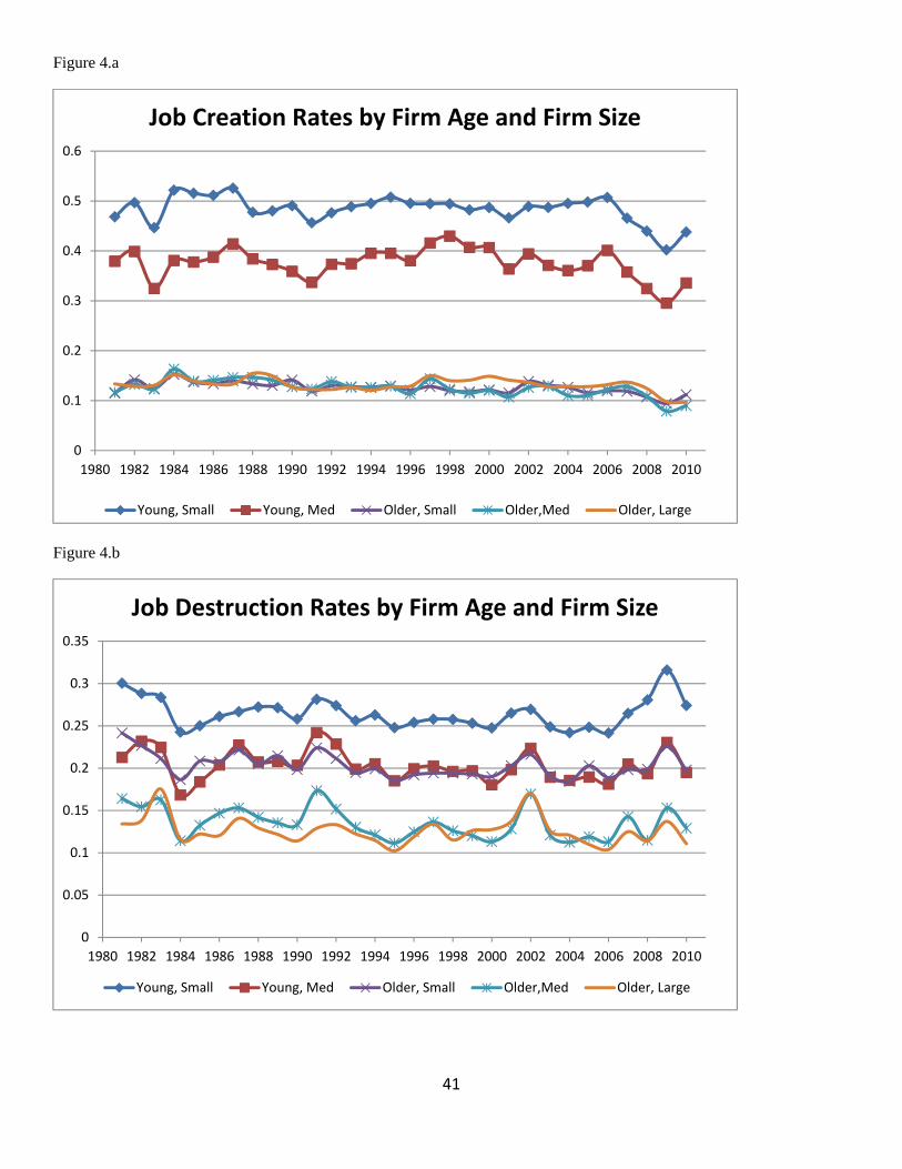
41
Figure 4.a
Figure 4.b
0
0.1
0.2
0.3
0.4
0.5
0.6
1980 1982 1984 1986 1988 1990 1992 1994 1996 1998 2000 2002 2004 2006 2008 2010
Job Creation Rates by Firm Age and Firm Size
Young, Small Young, Med Older, Small Older,Med Older, Large
0
0.05
0.1
0.15
0.2
0.25
0.3
0.35
1980 1982 1984 1986 1988 1990 1992 1994 1996 1998 2000 2002 2004 2006 2008 2010
Job Destruction Rates by Firm Age and Firm Size
Young, Small Young, Med Older, Small Older,Med Older, Large

42
Figure 5.1
Figure 5.2

43
Figure 5.3
Figure 5.4

44
Figure 5.5

45
Figure 6
Figure 7

46
Figure 8.a Job Creation Differential Response
Figure 8.b Job Destruction Differential Response

47
Figure 9.a. Net Differential Response for Construction
Figure 9.b Net Differential Response for Manufacturing

48
Figure 9.c Net Differential Response for Retail Trade
Figure 9.d Net Differential Response for Wholesale Trade

49
Figure 9.e Net Differential Response for FIRE
Figure 9.f Net Differentials for Services

50
Figure 9.g Net Differential Response for Transportation and Public Utilities

51
Appendix Tables and Figures
Figure A.1.1 Using State Net Employment Growth as Cyclical Indicator

52
Figure A.1.2 Using Net Employment Growth Rate for Cyclical Shock
Figure A.1.3 Using Net Employment Growth Rate for Cyclical Shock

53
Figure A.1.4 Using HP-filtered State Unemployment Rate
Figure A.1.5 Using HP-filtered State Unemployment Rate

54
Figure A.1.6.a Putting State Housing Prices Last in Causal Ordering
Figure A.1.6.b Putting State Housing Prices Last in Causal Ordering

55
Figure A.1.7 Using Initial Size
Figure A.1.8 Job Creation Differential Response for Young/Medium

56
Figure A.1.9 Job Destruction Differential Response for Young/Medium

57
Figure A.1.10 Using only Firm Age, Net Differential Response for Young (<5) Minus Old (5+)
Figure A.1.11 Using only Firm Size, Net Differential Response for Small/Medium (<500) Minus Large (500+)
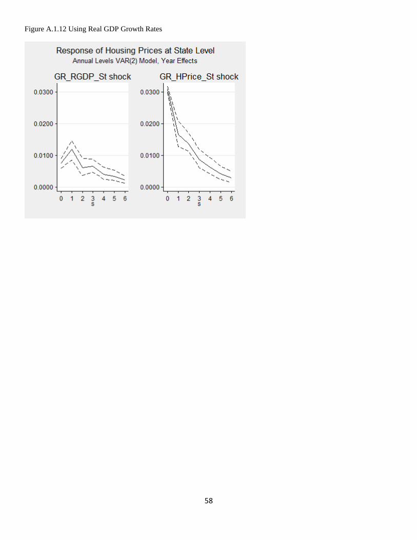
58
Figure A.1.12 Using Real GDP Growth Rates

59
Figure A.1.13 Using Real GDP Growth Rates
Figure A.1.14 Using Real GDP Growth Rates

60
Figure A.1.15 Using Real Personal Income Growth Rates
Figure A.1.16 Using Real Personal Income Growth Rates

61
Figure A.1.17 Using Growth Rates in Real Personal Income
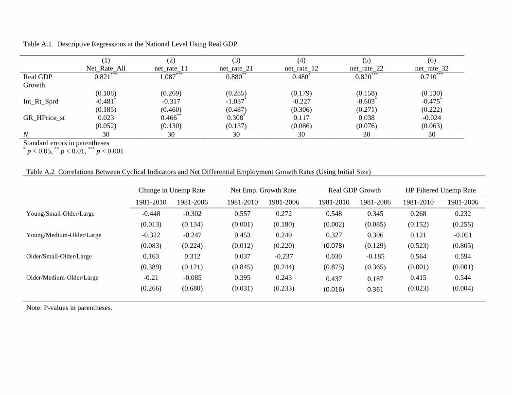
Table A.1. Descriptive Regressions at the National Level Using Real GDP
(1) (2) (3) (4) (5) (6) Net_Rate_All net_rate_11 net_rate_21 net_rate_12 net_rate_22 net_rate_32 Real GDP Growth
0.821*** 1.087*** 0.880** 0.480* 0.820*** 0.710***
(0.108) (0.269) (0.285) (0.179) (0.158) (0.130) Int_Rt_Sprd -0.481* -0.317 -1.037* -0.227 -0.603* -0.475* (0.185) (0.460) (0.487) (0.306) (0.271) (0.222) GR_HPrice_st 0.023 0.466** 0.308* 0.117 0.038 -0.024 (0.052) (0.130) (0.137) (0.086) (0.076) (0.063) N 30 30 30 30 30 30 Standard errors in parentheses * p < 0.05, ** p < 0.01, *** p < 0.001
Table A.2 Correlations Between Cyclical Indicators and Net Differential Employment Growth Rates (Using Initial Size)
Change in Unemp Rate Net Emp. Growth Rate Real GDP Growth HP Filtered Unemp Rate
1981-2010 1981-2006 1981-2010 1981-2006 1981-2010 1981-2006 1981-2010 1981-2006
Young/Small-Older/Large -0.448 -0.302 0.557 0.272 0.548 0.345 0.268 0.232
(0.013) (0.134) (0.001) (0.180) (0.002) (0.085) (0.152) (0.255)
Young/Medium-Older/Large -0.322 -0.247 0.453 0.249 0.327 0.306 0.121 -0.051
(0.083) (0.224) (0.012) (0.220) (0.078) (0.129) (0.523) (0.805)
Older/Small-Older/Large 0.163 0.312 0.037 -0.237 0.030 -0.185 0.564 0.594
(0.389) (0.121) (0.845) (0.244) (0.875) (0.365) (0.001) (0.001)
Older/Medium-Older/Large -0.21 -0.085 0.395 0.243 0.437 0.187 0.415 0.544
(0.266) (0.680) (0.031) (0.233) (0.016) 0.361 (0.023) (0.004)
Note: P-values in parentheses.

Table A.3 Descriptive Regressions at State Level, Using the Net Employment Growth Rate at state level as the cyclical indicator (Controlling for State and Year Fixed Effects)
Bivariate (1) (2) (3) (4) diff_net_rate_11 diff_net_rate_21 diff_net_rate_12 diff_net_rate_22 net_rate_st 0.559*** 0.224*** -0.241*** -0.209*** (0.058) (0.068) (0.038) (0.038) Multivariate (1) (2) (3) (4) diff_net_rate_11 diff_net_rate_21 diff_net_rate_12 diff_net_rate_22 net_rate_st 0.444*** 0.182* -0.320*** -0.263*** (0.061) (0.072) (0.040) (0.040) GR_HPrice_st 0.165*** 0.061 0.115*** 0.078*** (0.028) (0.034) (0.019) (0.019) N 1530 1530 1530 1530 Standard errors in parentheses * p < 0.05, ** p < 0.01, *** p < 0.001 Note 11=Young/Small, 21=Young/Medium, 12=Old/Small, 22=Old/Medium. All net differentials are with respect to Old/Large.
Table A.4 Descriptive Regressions at State Level, Using the Change in Unemployment Rate at state level as the cyclical indicator (Controlling for State Fixed Effects Only)
Bivariate (1) (2) (3) (4) diff_net_rate_11 diff_net_rate_21 diff_net_rate_12 diff_net_rate_22 Chg_UR_st -1.719*** -1.046*** 0.219* -0.409*** (0.135) (0.147) (0.088) (0.074) Multivariate (1) (2) (3) (4) diff_net_rate_11 diff_net_rate_21 diff_net_rate_12 diff_net_rate_22 Chg_UR_st -1.131*** -0.699*** 0.421*** -0.303*** (0.138) (0.156) (0.093) (0.079) GR_HPrice_st 0.309*** 0.182*** 0.106*** 0.055*** (0.026) (0.030) (0.018) (0.015) N 1530 1530 1530 1530 Standard errors in parentheses * p < 0.05, ** p < 0.01, *** p < 0.001 Note 11=Young/Small, 21=Young/Medium, 12=Old/Small, 22=Old/Medium. All net differentials are with respect to Old/Large.

64
Table A.5 Descriptive Regressions at State Level (Controlling for State and Year Fixed Effects) – Using State-Level Change in Unemployment Rate as Cyclical Indicator and Initial Firm Size
Bivariate (1) (2) (3) (4) diff_net_rate_11 diff_net_rate_21 diff_net_rate_12 diff_net_rate_22 Chg_UR_st -2.168*** -1.530*** -0.600*** -0.659*** (0.195) (0.271) (0.136) (0.137) Multivariate (1) (2) (3) (4) diff_net_rate_11 diff_net_rate_21 diff_net_rate_12 diff_net_rate_22 Chg_UR_st -1.846*** -1.496*** -0.495*** -0.596*** (0.195) (0.277) (0.139) (0.140) GR_HPrice_st 0.203*** 0.022 0.066*** 0.039* (0.025) (0.035) (0.018) (0.018) N 1530 1530 1530 1530 Standard errors in parentheses * p < 0.05, ** p < 0.01, *** p < 0.001 Note 11=Young/Small, 21=Young/Medium, 12=Old/Small, 22=Old/Medium. All net differentials are with respect to Old/Large.
Table A.6 Descriptive Regressions at State Level, Using the Real GDP Growth Rate at state level as the cyclical indicator (Controlling for State and Year Fixed Effects)
Bivariate (1) (2) (3) (4) diff_net_rate_11 diff_net_rate_21 diff_net_rate_12 diff_net_rate_22 GR_GDP_st 0.338*** 0.158*** 0.029 0.036 (0.040) (0.047) (0.027) (0.026) Multivariate (1) (2) (3) (4) diff_net_rate_11 diff_net_rate_21 diff_net_rate_12 diff_net_rate_22 GR_GDP_st 0.246*** 0.127* -0.008 0.018 (0.042) (0.050) (0.028) (0.028) GR_HPrice_st 0.171*** 0.057 0.068*** 0.033 (0.029) (0.034) (0.019) (0.019) N 1530 1530 1530 1530 Standard errors in parentheses * p < 0.05, ** p < 0.01, *** p < 0.001 Note 11=Young/Small, 21=Young/Medium, 12=Old/Small, 22=Old/Medium. All net differentials are with respect to Old/Large.

65
Table A.7 Descriptive Regressions at State Level, Using the Real Personal Income Growth Rate at state level as the cyclical indicator (Controlling for State and Year Fixed Effects)
Bivariate (1) (2) (3) (4) diff_net_rate_11 diff_net_rate_21 diff_net_rate_12 diff_net_rate_22 GR_RPI_st 0.658*** 0.391*** 0.114* 0.068 (0.066) (0.078) (0.044) (0.044) Multivariate (1) (2) (3) (4) diff_net_rate_11 diff_net_rate_21 diff_net_rate_12 diff_net_rate_22 GR_RPI_st 0.499*** 0.375*** 0.045 0.030 (0.076) (0.089) (0.051) (0.050) GR_HPrice_st 0.133*** 0.014 0.057** 0.032 (0.031) (0.036) (0.021) (0.020) N 1530 1530 1530 1530 Standard errors in parentheses * p < 0.05, ** p < 0.01, *** p < 0.001 Note 11=Young/Small, 21=Young/Medium, 12=Old/Small, 22=Old/Medium. All net differentials are with respect to Old/Large.


