
1
Hybrid Electrolytes with 3D Bicontinuous Ordered Ceramic and
Polymer Microchannels for All-Solid-State Batteries
Stefanie Zekoll#,1, Cassian Marriner-Edwards#,1, A. K. Ola Hekselman1,5, Jitti Kasemchainan1, Christian
Kuss1, David E. J. Armstrong1, Dongyu Cai2,3, Robert Wallace4, Felix H. Richter1,6, Job H. J. Thijssen2,
Peter G. Bruce1
#contributed equally
1Department of Materials, University of Oxford, Parks Road, Oxford, OX1 3PH, UK 2SUPA School of Physics and Astronomy, The University of Edinburgh, Edinburgh, EH9 3FD, UK
3 present address: Key Laboratory of Flexible Electronics (KLOFE) & Institute of Advanced Materials (IAM), Jiangsu National Synergetic Innovation Center for Advanced Materials (SICAM), Nanjing Tech
University, 30 South PuZhu Road, Nanjing, Jiangsu, 211816, China 4Department of Orthopaedics, The University of Edinburgh, Edinburgh, EH16 4SB, UK
5present address: Department of Materials, Imperial College London, London, SW7 2AZ, UK 6present address: Physikalisch-Chemisches Institut, Justus-Liebig-Universität Gießen, 35392 Gießen,
Germany
Sup1. Finite element modelling of designed microarchitectures
Electrochemical and mechanical properties of the three ordered microarchitectures (cube, diamond and
gyroid) have been modelled to predict their theoretically expected performances. All simulations were
performed with COMSOL Multiphysics 5.2 on a single repetition unit using periodic boundary conditions
perpendicular to the current flux or force.
Modelling of the ionic conduction in the structured hybrid electrolytes was carried out with COMSOL
electric currents physics, neglecting the effect of polarizability of the conductor on conduction and
assuming current contributions from only one charge carrier. A current flow was simulated by applying
the ground to one face of the cubic model geometry, whereas a potential was applied to the opposite
face. The extracted apparent mean conductivities of the hybrids can be used to evaluate the tortuosity
of conduction in these architectures as a normalized parameter. The table below shows these values
of tortuosity and the apparent conductivity reduction from the bulk LAGP phase for the three different
architectures at three different LAGP volume fractions of 50%, 70% and 85%. The experimentally
obtained conductivity reduction factor in the range of 0.4-0.7 for the structured hybrid electrolytes fits
very well with the predicted factor of about 0.6 (70 % volume fraction, table below).
Mechanical properties were modelled using COMSOL solid mechanics physics. Nanoindentation
showed an elastic modulus of 125 GPa for LAGP and a Poisson ratio of 0.25 was assumed. The
polypropylene phase elastic modulus was 0.9 GPa and Poisson ratio 0.421. Mechanical deformation
was simulated taking one face of the cube to be immobile, while elongating the cube at the opposite
face by 1%. The model shows an increase in elasticity of the structured hybrid electrolyte over bulk
LAGP, reducing the apparent elastic modulus by a factor of about 0.6 at 70% volume fraction of solid
electrolyte (table below).
1 C. H. Jenkins, S. K. Khanna, Mechanics of Materials, 1st ed., Academic Press, 2005.
Electronic Supplementary Material (ESI) for Energy & Environmental Science.This journal is © The Royal Society of Chemistry 2017

2
Figure Sup1.1 shows the modelled current density (top), and stress (bottom) distributions throughout
the structured hybrid electrolytes. The latter is quantified as equivalent tensile stress, or von Mises
stress, to account for the multidirectional load conditions in the hybrid structure according to von Mises’
failure theory.2 The cube microarchitecture clearly shows a significant volume of channels perpendicular
to current and strain, which contributes little to charge transport or stress distribution. Better spatial
dispersion of stress and current in the gyroid and diamond microarchitectures leads to a narrower
distribution of current and stress magnitudes, reducing the prevalence of high current density and high
von Mises stress, thus improving the overall conductivity and fracture resistance, respectively.
Table Sup1.1 Modelling of electrochemical and mechanical properties of the cube, gyroid and diamond microarchitectures.
Parameter Microarchitecture 50% LAGP 70% LAGP 85% LAGP LAGP
Tortuosity Cube 2.67 1.57 1.13 1 Gyroid 1.42 1.23 1.10 Diamond 1.41 1.22 1.11
Reduction in conductivity Cube 0.32 0.54 0.75 1
Gyroid 0.36 0.58 0.78 Diamond 0.35 0.58 0.76
Reduction in elastic modulus Cube 0.33 0.57 0.82 1
Gyroid 0.32 0.57 0.84 Diamond 0.28 0.57 0.83
2 R. von Mises, Göttin. Nachr. Math. Phys., 1913, 1, 582.

3
Figure Sup1.1 Normalized current density (top), and von Mises stress (bottom) distribution throughout the structured hybrid electrolytes in the 70% LAGP filling cube, diamond and gyroid microarchitectures shown as histograms (left) and colour maps (right). Histograms were created from a regular grid of 8000 probes of current density and stress throughout the microarchitectures.
4
Sup2. Synthesis procedure of a polymerized bijel
Bijels were prepared using a procedure similar to the one reported previously3 and is outlined here. 20
mg of silica nanoparticles of radius 63 nm (TEM) were dispersed in 0.70 mL of deionized water (Millipore
Milli-Q RG system, resistivity 18 Mcm) by ultrasonication (Sonics Vibracell) for (2 × 2) minutes
followed by (1 × 10) minutes at 8 W power, with 10 seconds of vortex mixing in between. 2,6-lutidine
(Aldrich, re-distilled, 99%) with 10 µM Nile Red was added to give a mixture with a 72:28 water:lutidine
mass ratio. Mixtures were transferred to 6 or 9 mm outer diameter glass cylinders glued onto glass
slides using Dow Corning Mono-Component Silicone Sealant. Samples were then heated inside a
microwave (DeLonghi, P80D20EL-T5A/H, 800 W), set to ‘auto-defrost’ for 5 or 9 seconds, after which
they were immediately transferred to a plastic incubator at 55 C. After 20 to 30 minutes, 20 or 60 L of
preheated monomer/initiator mixture (Sartomer SR238:initiator = 99:1 w/w) was added on top of each
sample.4 The monomer used was Sartomer SR238 and the initiator was 2-hydroxy-2-
methylpropiophenone (Aldrich, 97%). Samples were then transferred to an incubator at 55 C inside a
fume hood and sealed using vacuum grease and plastic lids. After about 4 h, samples were exposed
to UV light and cured both from the top and the bottom. Cured samples were removed from the cylinders
after twisting off the glass slides, the remaining liquids were drained using a paper tissue, after which
the samples were dried in the fume hood for at least 8 h. Finally, samples were further dried in a vacuum
oven (Gallenkamp) at 82 C for 1 h. Note that this bijel sample was micro-CT scanned to obtain a 3D
rendering, which was modified for use in 3D printing as outlined in the next section.
3 M. Reeves, K. Stratford, J. H. J. Thijssen, Soft Matter, 2016, 12, 4082. 4 M. Lee, A. Mohraz, Advanced Materials, 2010, 22, 4836.

5
Sup3. Design and printing of template microarchitectures
As the desired templates are too large to be printed without moving the sample stage, they are created
by stitching of smaller print blocks in a regular face-sharing arrangement. The print blocks are
themselves computationally designed as a multiple cubic arrangement of unit cells of the cube, gyroid
and diamond microarchitectures (Figure Sup3.1).
Figure Sup3.1 Development process of the unit cell, print block and template (left to right) as exemplified with the gyroid microarchitecture.
Cube, gyroid and diamond unit cell and print block generation
The gyroid unit cell is prepared using Matlab R2014b (8.4.0.150421) to generate the gyroid surface with
these input parameters:
a=2*π;
s=2*π/60;
[x,y,z]=meshgrid(-a:s:a,-a:s:a,-a:s:a);
cx = cos(2*x);
cy = cos(2*y);
cz = cos(2*z);
u = 50.0*(cos(x).*sin(y)+cos(y).*sin(z)+cos(z).*sin(x))-0.5*(cx.*cy+cy.*cz+cz.*cx)-52;
[f,v]=isosurface(u,0);
vertface2obj(v,f,'thinfig%.obj')
The surface is exported as a .obj file that is imported into Netfabb Professional (7.4.0). Using the repair
function, triangle faces are added to the open faces of the surface model creating a water-tight solid
model.
The diamond unit cell is prepared using OpenSCAD (2015.03-1) to generate the microarchitecture with
a shape radius of 0.33.
The cube unit cell is prepared using Netfabb Professional (7.4.0) to generate and arrange beams with
the desired properties. Further adjustments and repairs to the microarchitectures are carried out in
Netfabb Professional (7.4.0).

6
A 3x3x3 arrangement of the cubic unit cell and 2x2x2 arrangements of the gyroid and diamond unit
cells create the print blocks of the respective microarchitectures (Figure Sup3.2).
Bijel microarchitecture modification and print block generation
The print block of the bijel (Figure Sup3.2) is the CT scan of the polymerized bijel, modified
computationally as follows. The 3D rendering of the micro-CT scan of a polymerized bijel is
computationally sliced into a stack of 2D image files using Netfabb Professional (7.4.0). The image
stacks are imported into Avizo (9.1.1) and arranged as a 3D model. The auto-skeletisation operation
generated the medial axis of the model. The thickness of the line representing the medial axis is
adjusted to the required solid volume fraction. The medial axis model is then converted to a .stl file.
Trimming of the model is performed in Netfabb Professional (7.4.0).
Figure Sup3.2 Computationally designed print blocks (without print extensions) of the cube, gyroid, diamond and bijel-derived microarchitectures (left to right).
Print extensions for stitching
In order to have sufficient print block overlap for stitching, print extensions reaching into the
neighbouring print block section were added to the computational models as follows. Netfabb
Professional (7.4.0) was used to first import a prepared print block. A second print block was duplicated
and aligned adjacent to the original in order to maintain architectural continuity between the two. A
cutting operation was then used on the second print block 10 μm from the surface of the original print
block. The bulk of the cut block was then removed leaving behind the print extension. This process was
repeated for each side of the original print block before the separate shells were merged together to
generate the print block with print extensions.
3D laser lithography
DeScribe (2.3.4) was used to convert .stl files of different 3D print block architecture models to a print
ready .gwl file format. The sliced layer thickness and hatching distance of each of the architectures was
1 µm and 500 nm, respectively. The .gwl files were then imported to Nanowrite (1.8.3) and printed using
a Nanoscribe Photonics Professional GT as described in the experimental section.

7
Sup4. LAGP particle size after ball milling
Figure Sup4.1 SEM image of ball milled LAGP powder.

8
Sup5. LAGP powder filling of 3D printed templates
A number of liquids was tested to suspend the LAGP powder particles and to attempt to fill the 3D
printed template channels. Methanol proved to be the most effective at producing dense sediments
within the template channels and at yielding a negative replica of the 3D printed structures. Ethanol,
isopropanol and water also give acceptable filling results with LAGP, but diethyl ether, cyclohexane,
acetone and dimethyl sulfoxide do not work sufficiently well.
Figure Sup5.1 SEM images of the LAGP filled 3D printed templates with cube, gyroid, diamond and bijel-derived (left to right) microarchitectures. Methanol was used as dispersant for the LAGP powder.

9
Sup6. Extended version of Table 1 from main text
Table Sup6.1 Parameters that characterize the templates, structured LAGP scaffolds and structured hybrid electrolytes.
Cube Gyroid Diamond Bijel
Unit cell
Cubic unit cell dimension x=y=z / μm 80 105.6 121.9 240
Print block
Unit cells per print block in x, y, z direction 3x3x3 2x2x2 2x2x2 1x1x1
Cubic print block dimension x=y=z / μm 240 211.1 243.8 240
Template design
Print blocks per template design in x, y, z direction 5x5x10 6x6x12 5x5x10 5x5x10
Length x / mm 1.20 1.267 1.239 1.20
Length y / mm 1.20 1.267 1.239 1.20
Length z / mm 2.40 2.534 2.458 2.40
Volume / mm3 3.46 4.07 3.77 3.46
Printed Template Weight / mg 0.94 0.95 0.88 0.79
Length x / mm 1.20 1.26 1.21 1.19
Length y / mm 1.20 1.26 1.21 1.19
Length z / mm 2.40 2.51 2.41 2.39
Volume / mm3 3.46 3.98 3.53 3.38
Vol. shrinkage during printing / % 0 2 6 2
Template-LAGP Weight / mg 6.57 7.54 6.74 6.75
Length x / mm 1.25 1.30 1.24 1.26
Length y / mm 1.27 1.33 1.26 1.29
Length z / mm 2.53 2.66 2.55 2.57
Volume / mm3 4.02 4.60 3.98 4.18
Filled amount of LAGP / mg 5.63 6.59 5.86 5.96
Vol. expansion during filling / % 16 16 13 24
Str. LAGP scaffold Weight / mg 5.54 6.60 5.90 5.94
Length x / mm 1.03 1.11 1.10 1.06
Length y / mm 1.04 1.12 1.10 1.09
Length z / mm 2.12 2.24 2.14 2.16
Volume / mm3 2.27 2.78 2.59 2.50
Density / mg mm-3 2.44 2.37 2.28 2.38
Vol. shrinkage during sintering / % 44 40 35 40
Overall volume shrinkage / % 34 32 31 28
Str. LAGP-epoxy Weight / mg 5.34 6.36 5.08 5.66
Length x / mm 0.998 1.055 0.995 1.011
Length y / mm 1.002 1.067 0.997 1.010
Length z / mm 1.986 2.129 2.023 2.057
Volume / mm3 1.986 2.397 2.007 2.100
Density / mg mm-3 2.69 2.65 2.53 2.70
Str. LAGP-PP Weight / mg 5.58 6.61 5.62 5.84
Length x / mm 1.18 1.086 1.034 1.057
Length y / mm 1.036 1.073 1.053 1.061
Length z / mm 2.016 2.128 1.971 2.009
Volume / mm3 2.465 2.480 2.146 2.253
Density / mg mm-3 2.26 2.67 2.62 2.59
Template design Solid volume fraction / % 15.6 15.6 15.4 15.6
Str. LAGP scaffold Solid volume fraction / % 71.4 72.6 72.5 78.2
Template design Average empty channel size / μm 66.1 66.4 67.8 69.0
Str. LAGP scaffold Average LAGP thickness / μm 44.2 44.0 42.0 59.5
Template design Average wall thickness / μm 15.1 20.4 19.9 22.5
Str. LAGP scaffold Average empty channel size / μm 20.4 20.8 18.4 22.3

10
Sup7. Thickness vs. channel size distribution of template designs and structured LAGP
scaffolds
Figure Sup7.1 Histograms of empty channel diameter distribution of template designs (top) and LAGP thickness distribution of structured LAGP scaffolds (bottom).

11
Figure Sup7.2 Histograms of wall thickness distribution of template designs (top) and empty channel diameter distribution of structured LAGP scaffolds (bottom).

12
Sup8. SEM images of structured LAGP-PP electrolytes
Figure Sup8.1. SEM images of the structured LAGP-PP electrolytes with cube, gyroid, diamond and bijel-derived (left to right) microarchitectures.
13
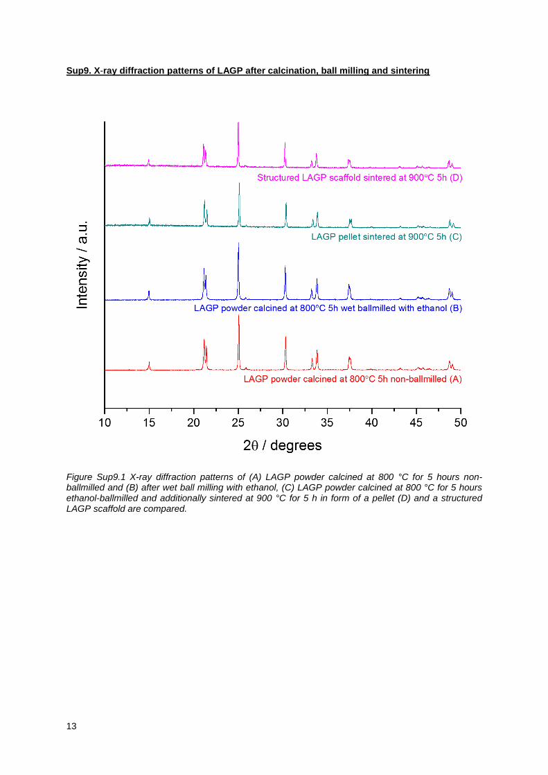
Sup9. X-ray diffraction patterns of LAGP after calcination, ball milling and sintering
Figure Sup9.1 X-ray diffraction patterns of (A) LAGP powder calcined at 800 °C for 5 hours non-ballmilled and (B) after wet ball milling with ethanol, (C) LAGP powder calcined at 800 °C for 5 hours ethanol-ballmilled and additionally sintered at 900 °C for 5 h in form of a pellet (D) and a structured LAGP scaffold are compared.

14
Sup10. Analysis of the Nyquist plots of cells with symmetric gold blocking electrodes
Both pellet and structured hybrid electrolytes were best fitted with an equivalent circuit consisting of a
resistor in series (R1), a combination of an ohmic resistor and constant-phase element (CPE) in parallel
(R2//CPE2) for the partially visible semicircle, and a serial CPE for the Au blocking electrodes (Figure
Sup10.1).
Figure Sup10.1 Equivalent circuit used to fit the Nyquist plots of LAGP and structured hybrid electrolytes with symmetric gold blocking electrodes at ambient temperature.
For all Nyquist plot fittings, a constant-phase element (CPE) (non-ideal capacitor taking into account
the slightly suppressed semicircles) was used. This deviation from an ideal R//C circuit is included in
the calculation of the capacitance values of the fittings. The complex impedance (ZCPE (ω)) as a function
of frequency (ω) can be represented by the following equation:
𝑍𝐶𝑃𝐸(𝜔) = 1
(𝑗𝜔)𝛼𝑄
where 𝑗 = √−1 and α and Q are CPE parameters.
Hence, the corresponding effective capacitance is calculated using following equation:
𝐶𝑒𝑓𝑓 = 𝑅(1−𝛼
𝛼)𝑄
1𝛼
where R is the resistor of the R//CPE circuit.
Full details of this derivation can be found in the work by Hirschorn et al.5 Tables Sup10.2 and Sup10.3
summarise the obtained and calculated parameters of the different contributions from the fitting of the
Nyquist plots of both pellet and structured hybrids at ambient temperature.
5 B. Hirschorn, M. E. Orazem, B. Tribollet, V. Vivier, I. Frateur and M. Musiani, Electrochim. Acta, 2010, 55, 6218–6227.

15
Table Sup10.1 EIS analysis of the LAGP pellet and gyroid hybrid electrolytes at ambient temperature without correcting for the difference in LAGP tortuosity and LAGP volume fraction.
R1 / Ω cm
Ceff1 / F cm-1
σ1 / S cm-1
f1 / Hz
R2 / Ω cm
Ceff2 / F cm-1
σ2 / S cm-1
f2 / Hz
σtot / S cm-1
Ea / kJ mol-1
LAGP pellet
2036 / 4.9 E-4 / 1484 9.9 E-11 6.7 E-4 1.1 E6 2.8 E-4 35.5
Gyroid LAGP-PP
2946 / 3.4 E-4 / 4525 5.9 E-11 2.2 E-4 6.0 E5 1.3 E-4 36.3
Gyroid LAGP-epoxy
3333 / 3.0 E-4 / 2964 1.0 E-10 3.4 E-4 5.4 E5 1.6 E-4 36.7
Table Sup10.2 EIS analysis of the LAGP pellet and gyroid hybrid electrolytes at ambient temperature with correcting for the difference in LAGP tortuosity and LAGP volume fraction by applying a correction factor derived from finite element modelling (for a 70% gyroid: 0.58).
R1 / Ω cm
Ceff1 / F cm-1
σ1 / S cm-1
f1 / Hz
R2 / Ω cm
Ceff2 / F cm-1
σ2 / S cm-1
f2 / Hz
σtot / S cm-1
Ea / kJ mol-1
LAGP pellet
2036 / 4.9 E-4 / 1484 9.9 E-11 6.7 E-4 1.1 E6 2.8 E-4 35.5
Gyroid LAGP-PP
1709 / 5.9 E-4 / 2625 3.4 E-11 3.8 E-4 6.0 E5 2.3 E-4 36.3
Gyroid LAGP-epoxy
1933 / 5.2 E-4 / 1719 5.8 E-11 5.8 E-4 5.4 E5 2.7 E-4 36.7
The impedance spectra at -30 °C were fitted with two parallel combinations of a resistor and a constant-
phase element (R1//CPE1 and R2//CPE2) in series, attributed to the two semicircles in the Nyquist plots,
and a constant-phase element (CPE3), attributed to the blocking interfaces between the Au electrodes
and the electrolyte. The equivalent circuit is shown in Figure Sup10.2.
Figure Sup10.2 Equivalent circuit used to fit the Nyquist plots of LAGP and structured hybrid electrolytes with symmetric gold blocking electrodes at -30 °C.
Tables Sup10.4 and Sup10.5 summarise the obtained and calculated parameters of the different
contributions from the fitting of the Nyquist plots of both pellet and structured hybrids at -30 °C.

16
Table Sup10.3 EIS analysis of the LAGP pellet and gyroid hybrid electrolytes at -30 °C without
correcting for the difference in LAGP tortuosity and LAGP volume fraction.
R1 / Ω cm
Ceff1 / F cm-1
σ1 / S cm-1
f1 / Hz
R2 / Ω cm
Ceff2 / F cm-1
σ2 / S cm-1
f2 / Hz
σtot / S cm-1
Ea / kJ mol-1
LAGP pellet
44390 1.10 E-11
2.25 E-5
3.27 E5
68296 1.82 E-10
1.46 E-5
1.28 E4
8.87 E-6
35.5
Gyroid LAGP-PP
54675 2.68 E-11
1.83 E-5
1.09 E5
84741 8.67 E-11
1.18 E-5
2.17 E4
7.17 E-6
36.3
Gyroid LAGP-epoxy
64797 7.40 E-12
1.54 E-5
3.32 E5
83485 9.67 E-11
1.20 E-5
1.97 E4
6.74 E-6
36.7
Table Sup10.4 EIS analysis of the LAGP pellet and gyroid hybrid electrolytes at -30 °C with correcting for the difference in LAGP tortuosity and LAGP volume fraction by applying a correction factor derived from finite element modelling (for a 70% gyroid: 0.58).
R1 / Ω cm
Ceff1 / F cm-1
σ1 / S cm-1
f1 / Hz
R2 / Ω cm
Ceff2 / F cm-1
σ2 / S cm-1
f2 / Hz
σtot / S cm-1
Ea / kJ mol-1
LAGP pellet
44390 1.10 E-11
2.25 E-5
3.27 E5
68296 1.82 E-10
1.46 E-5
1.28 E4
8.87 E-6
35.5
Gyroid LAGP-PP
31711 1.56 E-11
3.15 E-5
1.09 E5
49150 5.03 E-11
2.03 E-5
2.17 E4
1.24 E-5
36.3
Gyroid LAGP-epoxy
37582 4.30 E-12
2.66 E-5
3.32 E5
48421 5.61 E-11
2.07 E-5
1.97 E4
1.17 E-5
36.7

17
Sup11. Analysis of the Nyquist plots of cells with symmetric lithium electrodes
Electrochemical impedance measurements were performed on symmetrical cells assembled with
lithium metal electrodes of both pellet and gyroid hybrid electrolytes. The equivalent circuit used is
shown in Figure Sup11.1.
Figure Sup11.1 Equivalent circuit used to fit the Nyquist plots of LAGP and structured hybrid electrolytes with symmetric lithium electrodes at ambient temperature.
The Nyquist plots were best fitted using four parallel combinations of a resistor and a constant-phase
element in series (R1//CPE1, R2//CPE2, R3//CPE3 and R4//CPE4). The same equation as described in
Sup10 was used for the calculation of the effective capacitance. Tables Sup11.1 and Sup11.2
summarise the obtained and calculated parameters of the different contributions from the fitting of the
Nyquist plots of both pellet and gyroid hybrid electrolytes using symmetric lithium electrodes.
Table Sup11.1 EIS analysis of LAGP pellet and gyroid hybrid electrolyte cells assembled with symmetric lithium electrodes at room temperature without correcting for the difference in LAGP tortuosity and LAGP volume fraction.
R1 / Ω cm
Ceff1 / F cm-1
σ1 / S cm-1
f1 / Hz
R2 / Ω cm
Ceff2 / F cm-1
σ2 / S cm-1
f2 / Hz
LAGP pellet
1495 3.1 E-10 6.7 E-4 3.4 E5 1257 8.8 E-10 8.0 E-4 1.4 E5
Gyroid LAGP-PP
3284 2.1 E-10 3.1 E-4 2.3 E5 1232 1.3 E-9 8.1 E-4 9.6 E4
Gyroid LAGP-epoxy
2164 3.9 E-10 4.6 E-4 1.9 E5 1205 3.0 E-10 8.3 E-4 4.4 E5
R3 / Ω cm2
Ceff3 / F cm-2
σ3 / S cm-1
f1 / Hz
R4 / Ω cm2
Ceff4 / F cm-2
σ4 / S cm-1
f4 / Hz
σtot / S cm-1
LAGP pellet
34 1.4 E-8 1.9 E-3 2.3 E5 13 1.1 E-3 5.0 E-3 11.4 2.9 E-4
Gyroid LAGP-PP
71 2.9 E-8 1.1 E-3 7.7 E4 9 3.6 E-3 9.1 E-3 5.05 1.8 E-4
Gyroid LAGP-epoxy
171 1.2 E-8 3.7 E-4 7.6 E4 15 2.4 E-3 4.3 E-3 4.45 1.6 E-4

18
Table Sup11.2 EIS analysis of LAGP pellet and gyroid hybrid electrolyte cells assembled with symmetric
lithium electrodes at room temperature with correcting for the difference in LAGP tortuosity and LAGP
volume fraction by applying a correction factor derived from finite element modelling (for a 70% gyroid:
0.58) for the intragrain and intergrain contributions (R1//CPE1 and R2//CPE2) and with correcting for the
difference in LAGP area (for a 70% gyroid = 0.7) for the interphase layer and Li-LAGP interface
resistances (R3//CPE3 and R4//CPE4).
R1 / Ω cm
Ceff1 / F cm-1
σ1 / S cm-1
f1 / Hz
R2 / Ω cm
Ceff2 / F cm-1
σ2 / S cm-1
f2 / Hz
LAGP pellet
1495 3.1 E-10 6.7 E-4 3.4 E5 1257 8.8 E-10 8.0 E-4 1.4 E5
Gyroid LAGP-PP
1905 1.2 E-10 5.3 E-4 2.3 E5 715 7.5 E-10 1.4 E-3 9.6 E4
Gyroid LAGP-epoxy
1255 2.3 E-10 8.0 E-4 1.9 E5 699 1.7 E-10 1.4 E-3 4.4 E5
R3 / Ω cm2
Ceff3 / F cm-2
σ3 / S cm-1
f1 / Hz
R4 / Ω cm2
Ceff4 / F cm-2
σ4 / S cm-1
f4 / Hz
σtot / S cm-1
LAGP pellet
34 1.4 E-8 1.9 E-3 2.3 E5 13 1.1 E-3 5.0 E-3 11.4 2.9 E-4
Gyroid LAGP-PP
50 2.0 E-8 1.1 E-3 7.7 E4 6 2.5 E-3 9.1 E-3 5.05 3.0 E-4
Gyroid LAGP-epoxy
120 8.4 E-9 3.7 E-4 7.6 E4 11 1.7 E-3 4.3 E-3 4.45 2.5 E-4

19
Sup12. SEM and EDX analysis of the lithium-LAGP interphase layer formation
Figure Sup12.1 Charge and discharge curve, SEM images and EDX mapping of the cross-section of an LAGP pellet after 10 cycles at a constant current density of 1 mA cm-2 for 0.5h per charge and per discharge step.

20
Sup13. Galvanostatic cycling of cells of structured hybrid electrolytes assembled with
symmetric lithium electrodes: a comparison of microarchitectures and polymer filling
Figure Sup13.1 Galvanostatic cycling of structured LAGP-PP electrolytes (left column of plots) and structured LAGP-epoxy electrolytes (right column of plots), with cube, gyroid, diamond and bijel microarchitectures (top to bottom), assembled with lithium metal. Symmetrical cells were cycled at a constant current density of 1 mA/cm2 for 0.5 h per charge and per discharge step for a total of 10 cycles.

21
Sup14. Measurement parameters and impedance analysis of galvanostatic cycling
Using either the total electrode area or the LAGP phase area in contact with the lithium electrodes
allows for either a direct comparison of the overall sample performance or of the stability of the LAGP
phase at equal current density through the LAGP phase, respectively. The respective current density
and capacity values used in the experiments shown in the main paper are reported in the table below.
Table Sup14.1 List of measurement parameters used to obtain galvanostatic cycling data (Figure 8 of main text) of a LAGP pellet and gyroid LAGP-epoxy electrolytes assembled with symmetric lithium electrodes.
LAGP pellet
(Figure 8a)
Gyroid LAGP-epoxy (Figure 8b)
LAGP pellet
(Figure 8c)
Gyroid LAGP-epoxy (Figure 8d)
LAGP phase / % 100 70 100 70
Total area in contact with lithium / cm2 0.03142 0.03801 0.03801 0.03801
LAGP phase area in contact with lithium / cm2 0.03142 0.02661 0.03801 0.02661
Applied current / mA 0.02199 0.02661 0.03801 0.03801
Total areal current density jtotal / mA cm-2 0.7 0.7 1 1
LAGP phase current density jLAGP phase / mA cm-2 0.7 1 1 1.4
Applied capacity / mAh 0.011 0.013 0.019 0.019
Total areal capacity / mAh cm-2 0.35 0.35 0.5 0.5
LAGP phase areal capacity / mAh cm-2 0.35 0.5 0.5 0.7
Figure Sup14.1. Galvanostatic cycling of (a) LAGP pellet and (b) gyroid LAGP-epoxy electrolytes with
lithium electrodes cycled at an equal effective current density through the LAGP phase of 1.4 mA cm-2
(jLAGP phase) for 0.5 h per charge and discharge step.

22
Figure Sup14.2 Total resistance after each completed cycle for LAGP pellet and gyroid LAGP-epoxy
electrolytes cycled with symmetric lithium electrodes at current densities (jtotal) of (a) 0.7 mA cm-2 and
(b) 1 mA cm-2 and at equal effective current density through the LAGP phase (jLAGP phase) of (c) 1 mA cm-2
until the limiting voltage of the instrument is reached.
Figure Sup14.3 (a) Terminal voltage and (b) total resistance after each completed cycle for LAGP pellet
and gyroid LAGP-epoxy assembled with symmetric lithium electrodes at an effective current density
(jLAGP phase) of 1.4 mA cm-2 until the limiting voltage of the instrument is reached. LAGP pellet and gyroid
LAGP-epoxy achieve 12 and 20 cycles, respectively.

23
Sup15. CT analysis of pouched symmetric lithium cells before and after cycling
Figure Sup15.1 Micro-CT images of cross sections in parallel with the electrodes of symmetric lithium cells of gyroid LAGP-epoxy electrolyte (top) and LAGP pellet (bottom) before (left) and after (right) galvanostatic cycling at a constant current density of 1 mA cm-2 (using the total sample area of the electrolyte in contact with lithium) for 0.5 h per charge and discharge step for a total of 20 cycles.

24
Sup16. A LAGP cut-out of a LAGP pellet made for compression testing
Figure Sup16.1 SEM images of a cut-out of a LAGP pellet made for compression testing.
Table Sup6.2 List of structural parameters of a LAGP pellet cut-out.
Weight / mg 5.39
Length x / mm 0.930
Length y / mm 1.030
Length z / mm 1.936
Volume / mm3 1.854
Density / mg mm-3 2.91
25
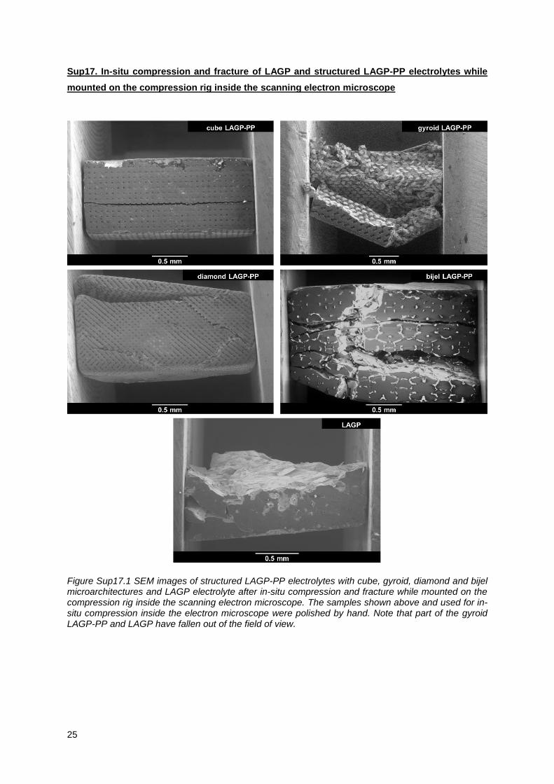
Sup17. In-situ compression and fracture of LAGP and structured LAGP-PP electrolytes while
mounted on the compression rig inside the scanning electron microscope
Figure Sup17.1 SEM images of structured LAGP-PP electrolytes with cube, gyroid, diamond and bijel microarchitectures and LAGP electrolyte after in-situ compression and fracture while mounted on the compression rig inside the scanning electron microscope. The samples shown above and used for in-situ compression inside the electron microscope were polished by hand. Note that part of the gyroid LAGP-PP and LAGP have fallen out of the field of view.
26
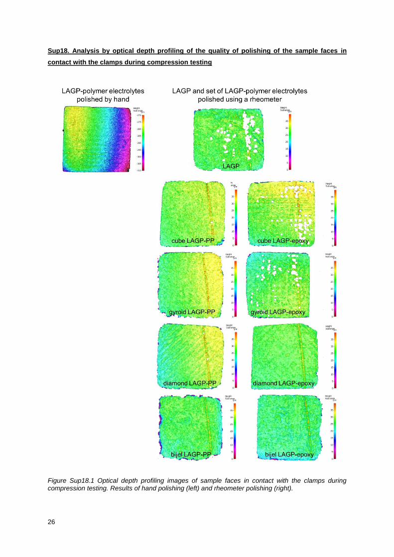
Sup18. Analysis by optical depth profiling of the quality of polishing of the sample faces in
contact with the clamps during compression testing
Figure Sup18.1 Optical depth profiling images of sample faces in contact with the clamps during compression testing. Results of hand polishing (left) and rheometer polishing (right).

27
Sup19. Evaluation of the elastic modulus from compression testing
Figure Sup19.1 Stress-strain curves obtained from strain rate controlled compression of LAGP vs. structured LAGP-epoxy electrolytes (left) and LAGP vs. structured LAGP-PP electrolytes (right) of approximately 1 mm x 1 mm x 2 mm in size starting from a preload of 50 N.
Table Sup19.1 Solid volume fraction obtained from micro-CT. Evaluation of the elastic modulus from the above stress-strain curves obtained from compression testing between 50 N and 150 N load.
cube gyroid diamond bijel LAGP
Solid volume fraction / % 71 73 73 78 ---
Elastic modulus LAGP-epoxy / GPa 47 44 41 51 63
Elastic modulus LAGP-PP / GPa 48 42 41 43
0.00
0.05
0.10
0.15
0.20
0.0 0.1 0.2 0.3
Co
mp
ressiv
e s
tre
ss / G
Pa
Compressive strain / %
LAGPcube LAGP-epoxygyroid LAGP-epoxydiamond LAGP-epoxybijel LAPG-epoxy
0.00
0.05
0.10
0.15
0.20
0.0 0.1 0.2 0.3
Co
mp
ressiv
e s
tre
ss / G
Pa
Compressive strain / %
LAGPcube LAGP-PPgyroid LAGP-PPdiamond LAGP-PPbijel LAGP-PP
28
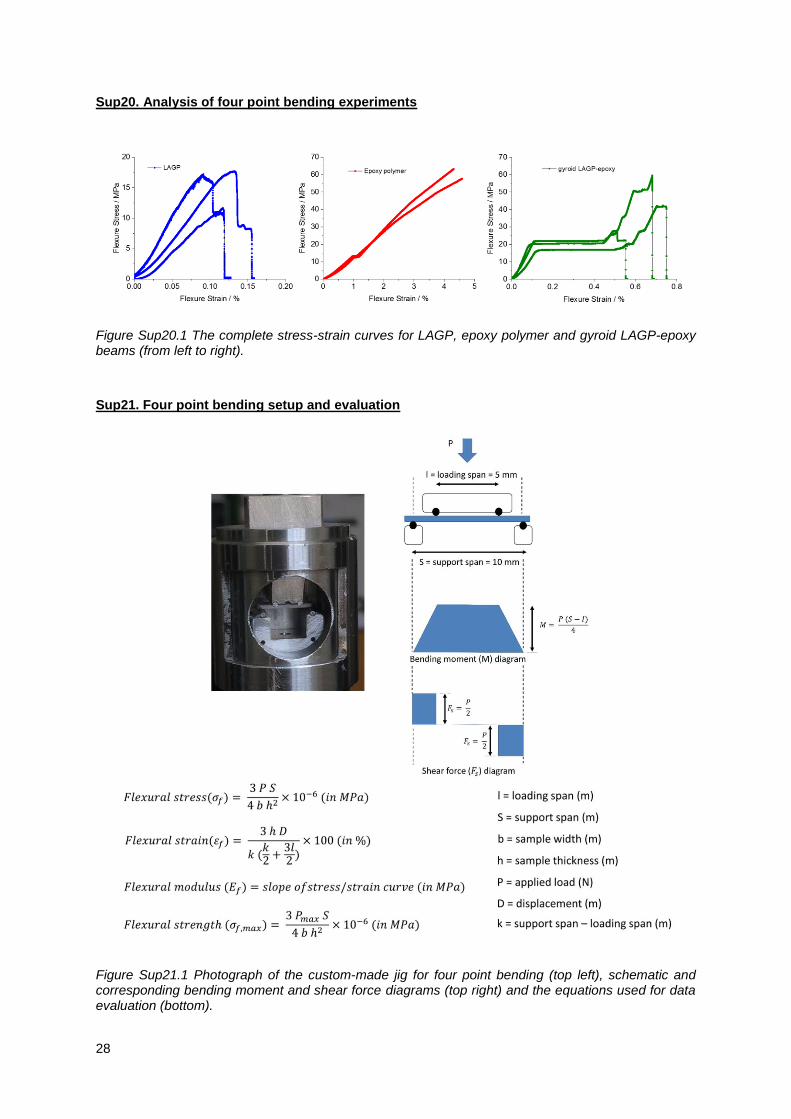
Sup20. Analysis of four point bending experiments
Figure Sup20.1 The complete stress-strain curves for LAGP, epoxy polymer and gyroid LAGP-epoxy beams (from left to right).
Sup21. Four point bending setup and evaluation
Figure Sup21.1 Photograph of the custom-made jig for four point bending (top left), schematic and corresponding bending moment and shear force diagrams (top right) and the equations used for data evaluation (bottom).


