Download - Hydrograph Analysis As Prepared By- - MMMUT

Hydrograph AnalysisAs Prepared By-
Dr. Saleh AlHassoun
1

HydrographRecord of River Discharge over a period of time ;
Q vs t
River Discharge : Q = AXv
= cross sectional area rivers mean (average) velocityX(at a particular point in its course)
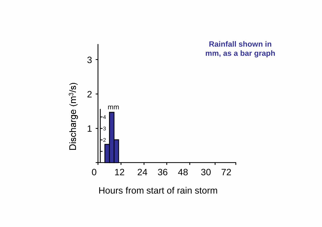
Storm HydrographsShow the change in discharge caused by a period of rainfall

Why Construct & AnalyseHydrographs ?
To find out discharge patterns ofa particular drainage basin
Help predict flooding events,therefore influence implementation of flood prevention measures
©Microsoft Word clipart

0 12 24 36 48 30 72 t(hrs)Hours from start of rain storm
___ Components of Streamflow___ Elements of Hydrograph
3
2
1
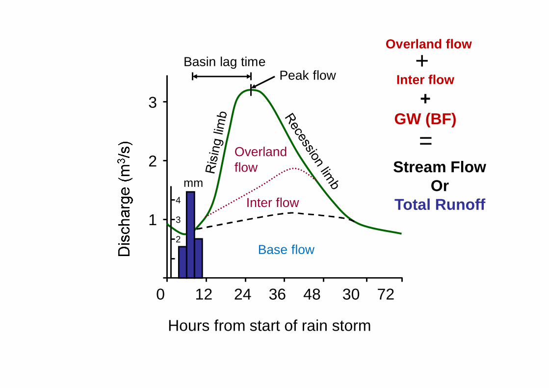
Base flow
Inter flow
Overland flow
Basin lag time
mm4
3
2
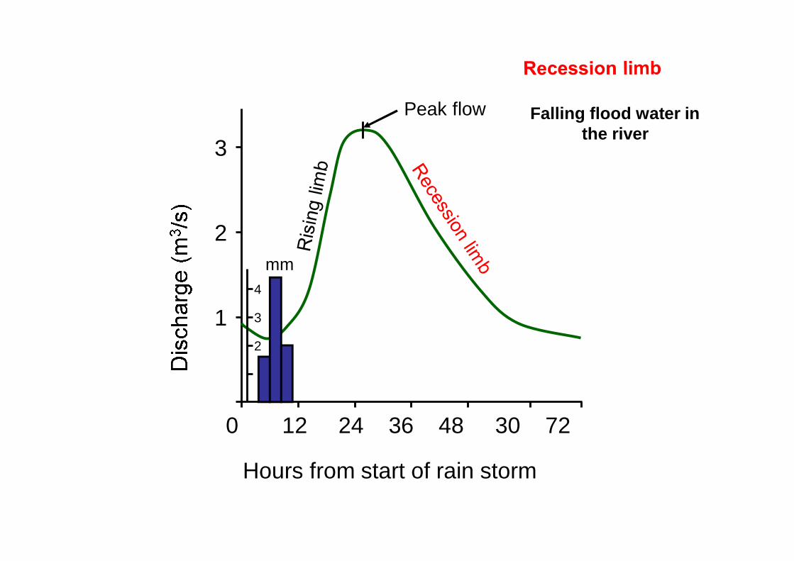
Peak flow (crest)

0 12 24 36 48 30 72
Hours from start of rain storm
3
2
1
0 12 24 36 48 30 72
Hours from start of rain storm
3
2
1
mm4
3
2
Rainfall shown in mm, as a bar graph

0 12 24 36 48 30 72
Hours from start of rain storm
3
2
1
mm4
3
2
Discharge in m3/s, as a line graph

0 12 24 36 48 30 72
Hours from start of rain storm
3
2
1
mm4
3
2
The rising flood water in the river

0 12 24 36 48 30 72
Hours from start of rain storm
3
2
1
mm4
3
2
Peak flow
Peak flow
Maximum discharge in the river
0 12 24 36 48 30 72
Hours from start of rain storm
3
2
1
mm4
3
2
Peak flow Falling flood water in the river

0 12 24 36 48 30 72
Hours from start of rain storm
3
2
1
Basin lag time
mm4
3
2
Peak flow
Basin lag time
Time difference between the peak of the rain storm and the peak
flow of the river

0 12 24 36 48 30 72
Hours from start of rain storm
3
2
1
Base flow
Basin lag time
mm4
3
2
Peak flow
Base flow
Normal discharge of the river
0 12 24 36 48 30 72
Hours from start of rain storm
3
2
1
Base flow
Inter flow
Overland flow
Basin lag time
mm4
3
2
Peak flow
Overland flow
Inter flow+
GW (BF)
+
=Stream Flow
OrTotal Runoff

Volume of water reaching the river from surface run off
GW
The Base flow
Overland flow Inter flow
Volume of water reaching the river through the soil and
underlying rock layers

Factors influencingStorm Hydrographs
• Area• Shape• Slope• Rock Type• Soil
• Land Use• Drainage Density• Precipitation / Temp• Tidal Conditions
©Microsoft Word clipart

Interpretation of Storm Hydrographs
•Rainfall Intensity
•Rising Limb•Recession Limb•Lag time
•Peak flow compared to Base flow•Recovery rate, back to Base flow
You need to refer to:Basin lag time
0 12 24 36 48 30 72
Hours from start of rain storm
3
2
1
Base flow
Through flow
Overland flow
mm
432
Peak flow

AreaLarge basins receive more precipitation than small therefore have larger runoff
Larger size means longer lag time as water has a longer distance to travel to reach the trunk river
Area Rock Type Drainage DensityShape Soil Precipitation / TempSlope Land Use Tidal Conditions

ShapeElongated basin will produce a lower peak flow and longer lag time than a circular
one of the same size
Area Rock Type Drainage DensityShape Soil Precipitation / TempSlope Land Use Tidal Conditions

SlopeChannel flow can be faster down a steep slope therefore steeper rising limb and
shorter lag time
Area Rock Type Drainage DensityShape Soil Precipitation / TempSlope Land Use Tidal Conditions

Rock TypePermeable rocks mean rapid infiltration and little overland flow therefore shallow
rising limb
Area Rock Type Drainage DensityShape Soil Precipitation / TempSlope Land Use Tidal Conditions

SoilInfiltration is generally greater on thick soil, although less porous soils eg. clay act
as impermeable layers
The more infiltration occurs the longer the lag time and shallower the rising limb
Area Rock Type Drainage DensityShape Soil Precipitation / TempSlope Land Use Tidal Conditions

Land UseUrbanisation - concrete and tarmac form impermeable surfaces, creating a steep
rising limb and shortening the time lag
Afforestation - intercepts the precipitation, creating a shallow rising limb and lengthening the time lag
Area Rock Type Drainage DensityShape Soil Precipitation / TempSlope Land Use Tidal Conditions

Drainage DensityA higher density will allow rapid overland flow
Area Rock Type Drainage DensityShape Soil Precipitation / TempSlope Land Use Tidal Conditions

Precipitation & TemperatureShort intense rainstorms can produce rapid overland flow and steep rising limb
If there have been extreme temperatures, the ground can be hard (either baked or frozen) causing rapid surface run off
Snow on the ground can act as a store producing a long lag time and shallow rising limb. Once a thaw sets in the rising limb will become steep
Area Rock Type Drainage DensityShape Soil Precipitation / TempSlope Land Use Tidal Conditions

Tidal ConditionsHigh spring tides can block the normal exit for the water, therefore extending the
length of time the river basin takes to return to base flow
Area Rock Type Drainage DensityShape Soil Precipitation / TempSlope Land Use Tidal Conditions

26
Hydrograph Analysis

27
Hydrograph Analysis :Hydrograph : Q vs t
• Duration , t• Lag Time , tL
• Time of Concentration , tc• Rising Limb• Recession Limb (falling limb)• Peak Flow ,Qp• Time to Peak (rise time),tp• Recession Curve• Base flow , BF• Separation of BF from Runoff

Hydrograph Components
Taken from Wanielista, M., R. Kersten, and R. Eaglin, Hydrology: Water Quantity and Quality Control, p. 184

29
Graphical Representation
Lag time
Time ofconcentration
Duration of excess precipitation.
Base flow

30
Separation of Baseflow
... generally accepted that the inflection point on the recession limb of a hydrograph is the result of a change in the controlling physical processes of the excess precipitation flowing to the basin outlet.
In this example, base flow is considered to be a straight line connecting that point at which the hydrograph begins to rise rapidly and the inflection point on the recession side of the hydrograph.
the inflection point may be found by plotting the hydrograph in semi-log fashion with flow being plotted on the log scale and noting the time at which the recession side fits a straight line.

31
Separation of Baseflow
0.0000
100.0000
200.0000
300.0000
400.0000
500.0000
600.0000
700.0000
Baseflow
Surface Response

32
Hydrograph & Baseflow
0
5000
10000
15000
20000
25000
Time (hrs.)

33
Separate Baseflow
0
5000
10000
15000
20000
25000
Time (hrs.)

Q = d * UH
Runoff = rainfall depth * Unit Hydrograph
34

35
Unit Hydrograph(UH) Theory:
• Sherman - 1932• Horton - 1933• Wisler & Brater - 1949 –
“the hydrograph of surface runoff resulting from a relatively short, intense rain, called a unit storm.”
• The runoff hydrograph may be “made up” of runoff that is generated as flow through the soil (Black, 1990).

36
Unit Hydrograph• The hydrograph (direct runoff)resulting from 1-
inch (or 1cm) of excess precipitation spread uniformly in space and time over a watershed for a given duration.
• The key points :
1-inch (1cm) of EXCESS precipitationSpread uniformly over space - evenly over the watershedUniformly in time - the excess rate is constant over the time intervalThere is a given duration. t-UH (ex. 2hr-UH)

37

38
Methods of Developing UH’s
• From Streamflow Data• Synthetically
– Snyder– SCS– Time-Area (Clark, 1945)
• “Fitted” Distributions• Geomorphologic

Unit Hydrograph Derivation• i) Tabulate the total hydrograph with time
distribution.• ii) Tabulate the baseflow if given or separate
with method of our choice.
• iii) Find the Direct Runoff Hydrograph(DRH)by subtracting the baseflow from the totalhydrograph.( DRH = Q – BF )
• iv) Find the volume of water under the DRH• Vol. = Q * t

40
Unit Hydrograph Derivation
0.0000
100.0000
200.0000
300.0000
400.0000
500.0000
600.0000
700.0000
0.0000 0.5000 1.0000 1 .5000 2 .0000 2 .5000 3.0000 3.5000 4.0000
Total H ydrograph
Surface R esponse
B aseflow

Unit Hydrograph Derivation• v) Divide the volume of water(step iv)
by the drainage area(A) to get effectiverainfall(de) (runoff) per unit area.
de = vol. / A
• vi) Divide the ordinates of the DRH bythe de of effective rainfall(step v).
• The result is a unit hydrograph(UH) forthe duration of storm.

42
Unit Hydrograph Derivation
0
0.1
0.2
0.3
0.4
0.5
0.6
0.7
0.8
0
5000
10000
15000
20000
25000
Time (hrs.)

43

0
2000
4000
6000
8000
10000
12000
0 5 10 15 20 25 30 35 40Time (hrs)
Plot of the Total Hydrograph

45
Obtain UH Ordinates
• The ordinates of the unit hydrograph are obtained by dividing each flow in the direct runoff hydrograph by the depth of excess precipitation.
• In this example, the units of the unit hydrograph would be cfs/inch (of excess precipitation).

46
Final UH
0
5000
10000
15000
20000
25000
Time (hrs.)
Storm #1 hydrograph
Storm#1 direct runoff hydrograph
Storm # 1 unit hydrograph
Storm #1 baseflow

47
Determine Duration of UH• The duration of the derived unit hydrograph is found by examining
the precipitation for the event and determining that precipitation which is in excess.
• This is generally accomplished by plotting the precipitation in hyetograph form and drawing a horizontal line such that the precipitation above this line is equal to the depth of excess precipitation as previously determined.
• This horizontal line is generally referred to as the -index and is based on the assumption of a constant or uniform infiltration rate.
• The uniform infiltration necessary to cause 1.65 inches of excess precipitation was determined to be approximately 0.2 inches per hour.

48
Estimating Excess Precip.
0
0.1
0.2
0.3
0.4
0.5
0.6
0.7
0.8
0 1 2 3 4 5 6 7 8 9 10 11 12 13 14 15 16 17 18 19
Time (hrs.)
Uniform loss rate of 0.2 inches per hour.

49
Excess Precipitation
0
0,1
0,2
0,3
0,4
0,5
0,6
0,7
0,8
0,9
1
0 1 2 3 4 5 6 7 8 9 10 11 12 13 14 15 16 17 18 19
Time (hrs.)
Small amounts of excess precipitation at beginning and end may
be omitted.
Derived unit hydrograph is the result of approximately 6 hours
of excess precipitation.

50
Changing the Duration
• Very often, it will be necessary to change the duration of the unit hydrograph.
• If unit hydrographs are to be averaged, then they must be of the same duration.
• Also, convolution of the unit hydrograph with a precipitation event requires that the duration of the unit hydrograph be equal to the time step of the incremental precipitation.
• The most common method of altering the duration of a unit hydrograph is by the S-curve method.
• The S-curve method involves continually lagging a unit hydrograph by its duration and adding the ordinates.
• For the present example, the 6-hour unit hydrograph is continually lagged by 6 hours and the ordinates are added.

51

52

53

54
Develop S-Curve
0,00
10000,00
20000,00
30000,00
40000,00
50000,00
60000,00
Time (hrs.)

55
Convert to 1-Hour Duration• To arrive at a 1-hour unit hydrograph, the S-curve is lagged
by 1 hour and the difference between the two lagged S-curves is found to be a 1 hour unit hydrograph.
• However, because the S-curve was formulated from unit hydrographs having a 6 hour duration of uniformly distributed precipitation, the hydrograph resulting from the subtracting the two S-curves will be the result of 1/6 of an inch of precipitation.
• Thus the ordinates of the newly created 1-hour unit hydrograph must be multiplied by 6 in order to be a true unit hydrograph.
• The 1-hour unit hydrograph should have a higher peak which occurs earlier than the 6-hour unit hydrograph.
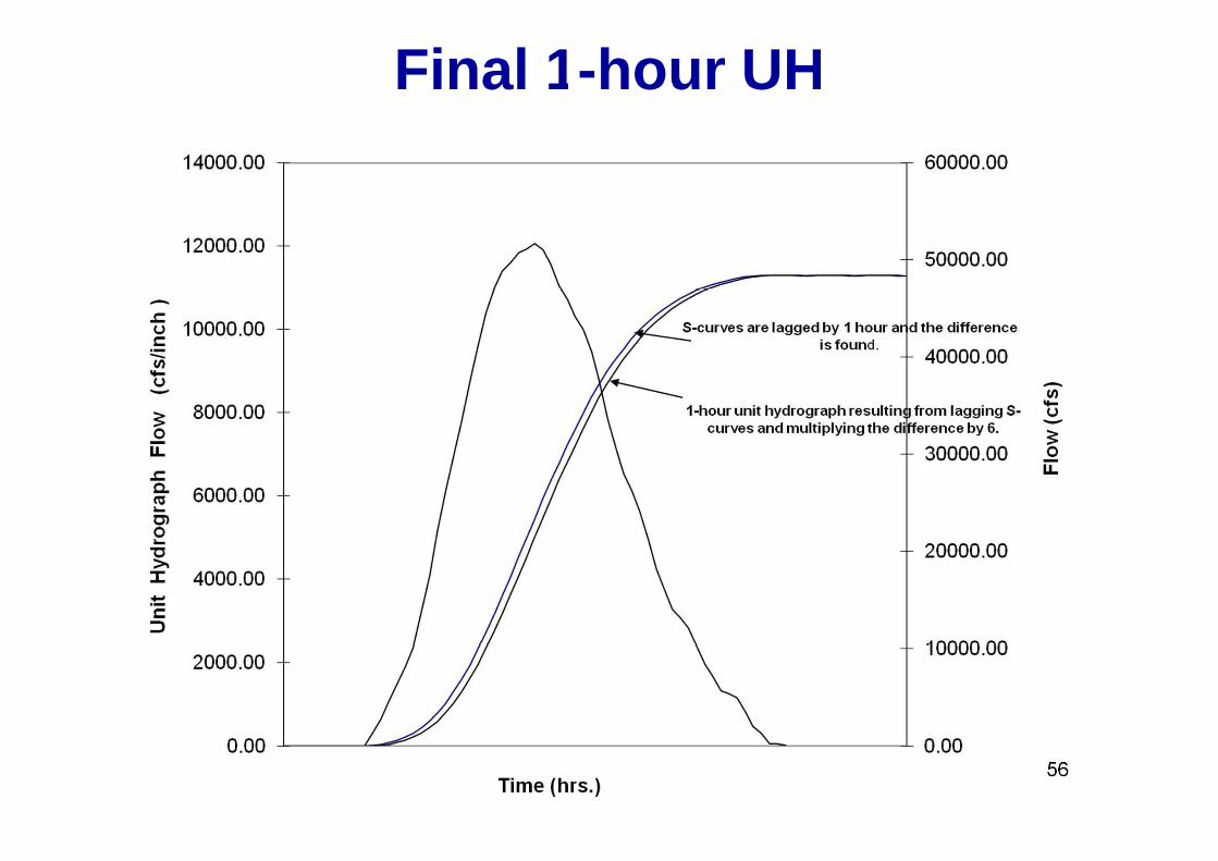
56
Final 1-hour UH

57
Shortcut Method•There does exist a shortcut method for changing the duration of the unit hydrograph if the two durations are multiples of one another.
•This is done by displacing the the unit hydrograph.
•For example, if you had a two hour unit hydrograph and you wanted to change it to a four hour unit hydrograph.

58
Shortcut Method Example
Time (hr) Q0 01 22 43 64 105 66 47 38 29 110 0
•First, a two hour unit hydrograph is given and a four hour unit hydrograph is needed. •There are two possibilities, develop the S - curve or since they are multiples use the shortcut method.

59
Shortcut Method Example•The 2 hr-UH is then displaced by 2 hours. •This is done because the 2 hr-UH will be used to represent
a 4 hr-UH.Time (hr) Q Displaced UHG
0 01 22 4 03 6 24 10 45 6 66 4 107 3 68 2 49 1 310 0 211 112 0

60
Shortcut Method Example•These two hydrographs are then summed.
Time (hr) Q Displaced UHG Sum0 0 01 2 22 4 0 43 6 2 84 10 4 145 6 6 126 4 10 147 3 6 98 2 4 69 1 3 410 0 2 211 1 112 0 0

61
Shortcut Method Example•Finally the summed hydrograph is divided by two.•This is done because when two unit hydrographs are added, the area under the curve is two units. This has to be reduced back to one unit of runoff.
Time (hr) Q Displaced UHG Sum 4 hour UHG0 0 0 01 2 2 12 4 0 4 23 6 2 8 44 10 4 14 75 6 6 12 66 4 10 14 77 3 6 9 4.58 2 4 6 39 1 3 4 210 0 2 2 111 1 1 0.512 0 0 0

62
Average Several UH’s• It is recommend that several unit hydrographs be derived
and averaged.• The unit hydrographs must be of the same duration in order
to be properly averaged.• It is often not sufficient to simply average the ordinates of
the unit hydrographs in order to obtain the final unit hydrograph. A numerical average of several unit hydrographs which are different “shapes” may result in an “unrepresentative” unit hydrograph.
• It is often recommended to plot the unit hydrographs that are to be averaged. Then an average or representative unit hydrograph should be sketched or fitted to the plotted unit hydrographs.
• Finally, the average unit hydrograph must have a volume of 1 inch of runoff for the basin.

63
Synthetic UHG’s• Snyder• SCS• Time-area• IHABBS Implementation Plan :
NOHRSC Homepagehttp://www.nohrsc.nws.gov/
http://www.nohrsc.nws.gov/98/html/uhg/index.html

64
Snyder• Since peak flow and time of peak flow are two of the
most important parameters characterizing a unit hydrograph, the Snyder method employs factors defining these parameters, which are then used in the synthesis of the unit graph (Snyder, 1938).
• The parameters are Cp, the peak flow factor, and Ct, the lag factor.
• The basic assumption in this method is that basins which have similar physiographic characteristics are located in the same area will have similar values of Ct and Cp.
• Therefore, for ungaged basins, it is preferred that the basin be near or similar to gaged basins for which these coefficients can be determined.

65
Basic Relationships3.0)( catLAG LLCt
5.5LAG
durationtt
83 LAG
basett
LAG
ppeak t
ACq
640
66
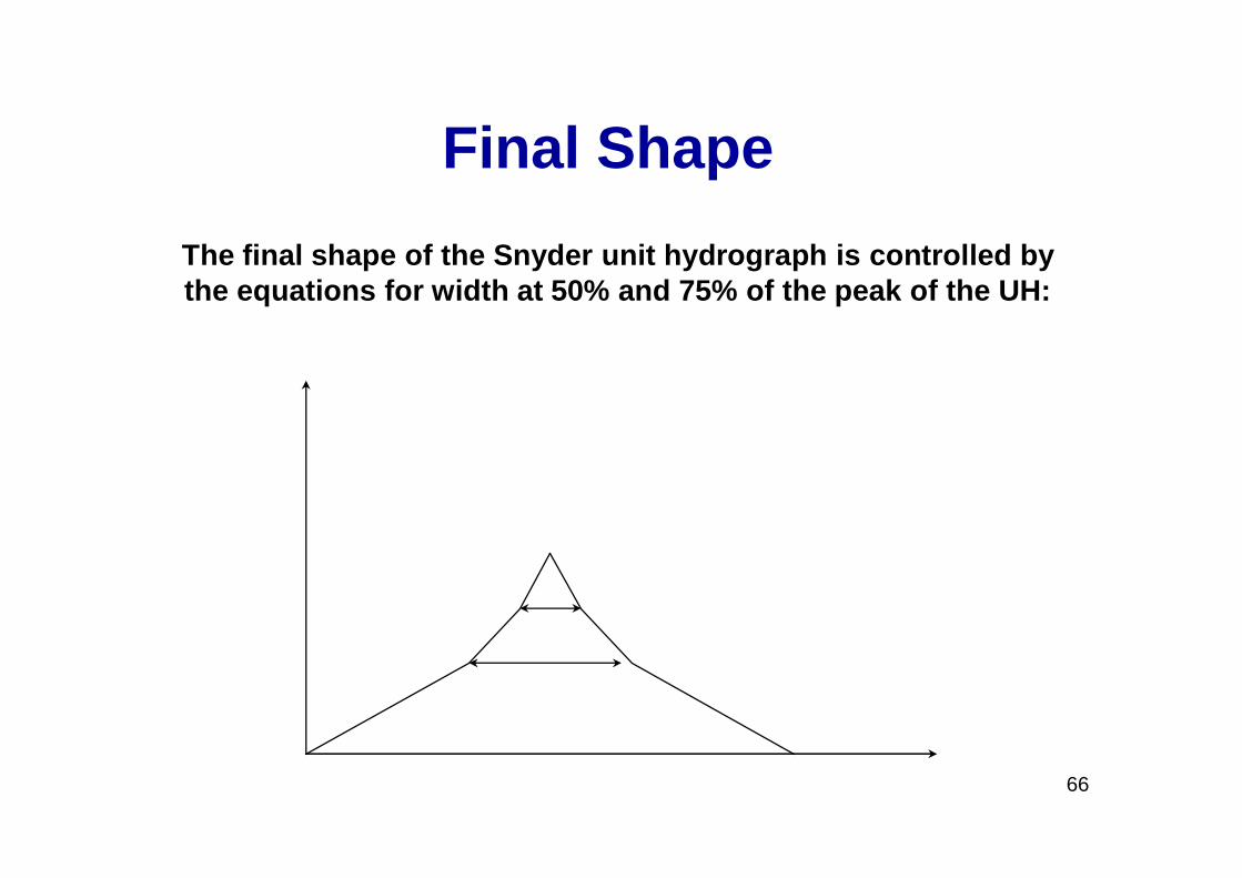
Final ShapeThe final shape of the Snyder unit hydrograph is controlled by the equations for width at 50% and 75% of the peak of the UH:

67
SCS
SCS Dimensionless UHG Features
0
0.2
0.4
0.6
0.8
1
0 0.5 1 1.5 2 2.5 3 3.5 4 4.5 5T/Tpeak
Flow ratios
Cum. Mass

68
Dimensionless RatiosTime Ratios
(t/tp)Discharge Ratios
(q/qp)Mass Curve Ratios
(Qa/Q)0 .000 .000.1 .030 .001.2 .100 .006.3 .190 .012.4 .310 .035.5 .470 .065.6 .660 .107.7 .820 .163.8 .930 .228.9 .990 .300
1.0 1.000 .3751.1 .990 .4501.2 .930 .5221.3 .860 .5891.4 .780 .6501.5 .680 .7001.6 .560 .7511.7 .460 .7901.8 .390 .8221.9 .330 .8492.0 .280 .8712.2 .207 .9082.4 .147 .9342.6 .107 .9532.8 .077 .9673.0 .055 .9773.2 .040 .9843.4 .029 .9893.6 .021 .9933.8 .015 .9954.0 .011 .9974.5 .005 .9995.0 .000 1.000

69
Triangular Representation
SCS Dimensionless UHG & Triangular Representation
0
0.2
0.4
0.6
0.8
1
1.2
0.0 1.0 2.0 3.0 4.0 5.0
T/Tpeak
Flow ratiosCum. MassTriangular
Excess Precipitation
D
Tlag
Tc
TpTb
Point of Inflection

70
Triangular Representationpb T x 2.67 T
ppbr T x 1.67 T - T T
)T + T( 2q
= 2Tq
+ 2Tq
= Q rpprppp
T + T2Q = q
rpp
T + TQ x A x 2 x 654.33 = q
rpp The 645.33 is the conversion used for
delivering 1-inch of runoff (the area under the unit hydrograph) from 1-square
mile in 1-hour (3600 seconds).T
Q A 484 = qp
p
SCS Dimensionless UHG & Triangular Representation
0
0.2
0.4
0.6
0.8
1
1.2
0.0 1.0 2.0 3.0 4.0 5.0
T/Tpeak
Flow ratiosCum. MassTriangular
Excess Precipitation
D
Tlag
Tc
TpTb
Point of Inflection

71
484 ?
Comes from the initial assumption that 3/8 of the volume under the UHG is under the rising limb and the remaining 5/8
is under the recession limb.
General Description Peaking Factor Limb Ratio(Recession to Rising)
Urban areas; steep slopes 575 1.25Typical SCS 484 1.67
Mixed urban/rural 400 2.25Rural, rolling hills 300 3.33Rural, slight slopes 200 5.5
Rural, very flat 100 12.0
TQ A 484 = q
pp

72
Duration & Timing?
L + 2D = T p
cTL *6.0L = Lag time
pT 1.7 D Tc
T = T 0.6 + 2D
pc
For estimation purposes : cT 0.133 D
Again from the triangle

73
Time of Concentration
• Regression Eqs.• Segmental Approach

74
A Regression Equation
TlagL S
Slope
08 1 0 7
1900 05
. ( ) .
(% ) .
where : Tlag = lag time in hoursL = Length of the longest drainage path in feetS = (1000/CN) - 10 (CN=curve number)%Slope = The average watershed slope in %

75
Segmental Approach• More “hydraulic” in nature• The parameter being estimated is essentially the time of
concentration or longest travel time within the basin.• In general, the longest travel time corresponds to the longest
drainage path• The flow path is broken into segments with the flow in each segment
being represented by some type of flow regime.• The most common flow representations are overland, sheet, rill and
gully, and channel flow.

76
A Basic Approach 21
kSV
McCuen (1989) and SCS (1972) provide values of k for several flow situations
(slope in %)
K Land Use / Flow Regime0.25 Forest with heavy ground litter, hay meadow (overland flow)0.5 Trash fallow or minimum tillage cultivation; contour or strip
cropped; woodland (overland flow)0.7 Short grass pasture (overland flow)0.9 Cultivated straight row (overland flow)1.0 Nearly bare and untilled (overland flow); alluvial fans in
western mountain regions1.5 Grassed waterway2.0 Paved area (sheet flow); small upland gullies
Flow Type KSmall Tributary - Permanent or intermittent
streams which appear as solid or dashedblue lines on USGS topographic maps.
2.1
Waterway - Any overland flow route whichis a well defined swale by elevation
contours, but is not a stream section asdefined above.
1.2
Sheet Flow - Any other overland flow pathwhich does not conform to the definition of
a waterway.
0.48
Sorell & Hamilton, 1991

77
Triangular Shape• In general, it can be said that the triangular version will not cause or
introduce noticeable differences in the simulation of a storm event, particularly when one is concerned with the peak flow.
• For long term simulations, the triangular unit hydrograph does have a potential impact, due to the shape of the recession limb.
• The U.S. Army Corps of Engineers (HEC 1990) fits a Clark unit hydrograph to match the peak flows estimated by the Snyder unit hydrograph procedure.
• It is also possible to fit a synthetic or mathematical function to the peak flow and timing parameters of the desired unit hydrograph.
• Aron and White (1982) fitted a gamma probability distribution using peak flow and time to peak data.

78
Fitting a Gamma Distribution
)1(),;(
1 abetbatf
a
bta
0.0000
50.0000
100.0000
150.0000
200.0000
250.0000
300.0000
350.0000
400.0000
450.0000
500.0000
0.0000 1.0000 2.0000 3.0000 4.0000 5.0000 6.0000

79
Time-Area

80
Time-Area
Time
Q % Area
Time
100%
Timeof conc.

81
Time-Area

82
Hypothetical Example• A 190 mi2 watershed is divided into 8 isochrones of travel time.• The linear reservoir routing coefficient, R, estimated as 5.5 hours. • A time interval of 2.0 hours will be used for the computations.
234
5
66
7
8
6
5
7
7
10

83
Rule of Thumb
R - The linear reservoir routing coefficient can be estimated as approximately 0.75
times the time of concentration.

84
Basin Breakdown
MapArea #
BoundingIsochrones
Area(mi2)
CumulativeArea (mi2)
CumulativeTime (hrs)
1 0-1 5 5 1.02 1-2 9 14 2.03 2-3 23 37 3.04 3-4 19 58 4.05 4-5 27 85 5.06 5-6 26 111 6.07 6-7 39 150 7.08 7-8 40 190 8.0
TOTAL 190 190 8.0
234
5
66
7
8
6
5
7
7
10

85
Incremental Area
0
5
10
15
20
25
30
35
40
1 2 3 4 5 6 7 8Time Increment (hrs)
234
5
66
7
8
6
5
7
7
10
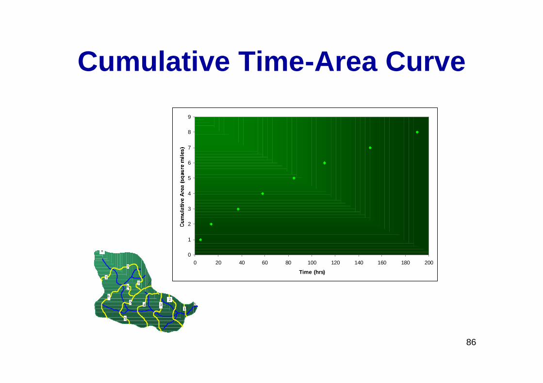
86
Cumulative Time-Area Curve
0
1
2
3
4
5
6
7
8
9
0 20 40 60 80 100 120 140 160 180 200
Time (hrs)
234
5
66
7
8
6
5
7
7
10

87
Trouble Getting a Time-Area Curve?
0.5) Ti (0for 414.1 5.1ii TTA
1.0) Ti (0.5for )1(414.11 5.1ii TTA
Synthetic time-area curve -The U.S. Army Corps of Engineers (HEC 1990)

88
Instantaneous UHG
)1()1( iii IUHccIIUH
tRtc
22
t = the time step used n the calculation of the translation unit hydrographThe final unit hydrograph may be found by averaging 2 instantaneous unit hydrographs that are a t time step apart.

89
ComputationsTime(hrs)
(1)
Inc.Area(mi2)(2)
Inc.TranslatedFlow (cfs)
(3)
Inst. UHG
(4)
IUHGLagged 2
hours(5)
2-hrUHG(cfs)(6)
0 0 0 0 02 14 4,515 1391 0 7004 44 14,190 5333 1,391 3,3606 53 17,093 8955 5,333 7,1508 79 25,478 14043 8,955 11,50010 0 0 9717 14,043 11,88012 6724 9,717 8,22014 4653 6,724 5,69016 3220 4,653 3,94018 2228 3,220 2,72020 1542 2,228 1,89022 1067 1,542 1,30024 738 1,067 90026 510 738 63028 352 510 43030 242 352 30032 168 242 20034 116 168 14036 81 116 10038 55 81 7040 39 55 5042 26 39 3044 19 26 2046 13 19 2048 13

90
Incremental Areas
0
10
20
30
40
50
60
70
80
90
0 2 4 6 8 10
Time Increments (2 hrs)

91
Incremental Flows
0
5000
10000
15000
20000
25000
30000
1 2 3 4 5 6
Time Increments (2 hrs)

92
Instantaneous UHG
0
2000
4000
6000
8000
10000
12000
14000
16000
0 10 20 30 40 50 60
Time (hrs)
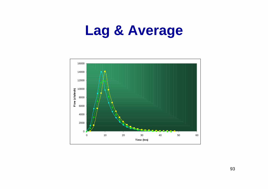
93
Lag & Average
0
2000
4000
6000
8000
10000
12000
14000
16000
0 10 20 30 40 50 60
Time (hrs)

Engineering Hydrology
-1
BY-
Dr. Yunes MogheirDr. Ramadan Al Khatib

Previous Chapter estimation of long-term runoff was examined
the present chapter examines in detail the short-term runoff phenomenon by the storm hydrograph or flood hydrograph or simply Hydrograph
The runoff measured at the stream-gauging station will give a typical hydrograph as shown in Fig. 6.1

- The flood hydrograph is formed as a result of uniform rainfall of duration, Tr,. over a catchment.
- The Hydrograph (Figure 6.1) has three characteristic regions: (i) the rising limb AB, joining point A, the starting point of the rising curve and point B, the point of inflection, (ii) the crest segment BC between the two points of inflection with a peak P in between, (iii) the falling limb or depletion curve CDstarting from the second point of inflection C.

- Timing of the Hydrograph1. tpk : the time to peak (Qp) from the starting point A, 2. lag time TL : the time interval from the centre of
mass of rainfall to the centre of mass of hydrograph,
3. TB : the time base of the hydrograph
- Factor Influencing the Hydrograph1. Watershed Characteristics such as
size, shape, slope, storage2. Infiltration Characteristics
soil and land use and cover 3. Climactic Factors
- rainfall intensity and pattern- aerial distribution- duration- type (rainfall vs snowmelt)
- Generally, the climatic factors control the rising limb
- catchment characteristics determine the recession limb

the essential components of a hydrograph are: (i) the rising limb,(ii) the crest segment, and (iii) the recession limb.
D.R.
baseflow
Falling limb
crest
Rising
limb
Q (m3/s)
TimeConcentration
curveRecession
curve
6.3 COMPONENTS OF A HYDROGRAPH
Inflection Point

Rising Limb
The rising limb of a hydrograph (concentration curve) represents the increase in discharge due to the gradual building up of storage in channels and over the catchment surface. As the storm continues more and more flow from distant parts reach the basin outlet. At the same time the infiltration losses also decrease with time.
Crest The peak flow occurs when the runoff from various parts of the catchment at the same time contribute the maximum amount of flow at the basin outlet.Generally for large catchments, the peak flow occurs after the end of rainfall,the time interval from the centre of mass of rainfall to the peak being essentially controlled by basin and storm characteristics.

Recession LimbIt extends from the point of inflection at the end of the crest segment to the start of the natural groundwater flow
It represents the withdrawal of water from the storage built up in the basin during the earlier phases of the hydrograph.
The starting point of the recession limb (the point of inflection)represents the condition of maximum storage.
Since the depletion of storage takes place after the end of rainfall, the shape of this part of the hydrograph is independent of storm characteristics and depends entirely on the basin characteristics.
The storage of water in the basin exists as - surface storage, which includes both surface detention and
channel storage, -interflow storage, and -groundwater storage, i.e. base-flow storage.

Barnes (1940) showed that the recession of a storage can be expressed as
which Q0: the initial discharge and Qt :are discharges at a time interval of t days; K: is a recession constant of value less than unity.
Previous Equation can also be expressed in an alternative form of the exponential decay as
where a =-In K,
The recession constant K; can be considered to be made up of three components to take care of the three types of storages as:K= Krs . Kri . Krb
where Krs = recession constant for surface storage (0.05 to 0.20), Kri= recession constant for interflow (0.50 to 0.85) and
Krb = recession constant for base flow (0.85 to 0.99)
Example 6.1

- The surface hydrograph is obtained from the total storm hydrograph by separating the quick-response flow from the slow response runoff.
- The base flow is to be deducted from the total storm hydrograph to obtain the surface flow hydrograph in three methods

- Draw a horizontal line from start of runoff to intersection with recession limb (Point A).
- Extend from time of peak to intersect with recession limb using a lag time, N.
N =0.83 A0.2
Where: A = the drainage area in Km2 and N = days where Point B can be located and determine the end ofthe direct runoff .
Method I: Straight line method

Method II:- In this method the base flow curve existing prior to the beginning of the
surface runoff is extended till it intersects the ordinate drawn at the peak (point C in Fig, 6.5). This point is joined to point B by a straight line.
- Segment AC and CB separate the base flow and surface runoff.
- This is probably the most widely used base-flow separation procedure.
time
QN
AB
C

- In this method the base flow recession curve after the depletion of the flood water is extended backwards till it intersects the ordinate at the point of inflection (line EF in Fig. 6.5), Points A and F are joined by an arbitrary smooth curve.
- This method of base-flow separation is realistic in situations where the groundwater contributions are significant and reach the stream quickly.
- The selection of anyone of the three methods depends upon the local practice and successful predictions achieved in the past.
- The surface runoff hydrograph obtained after the base-flow separation is also known as direct runoff hydrograph (DRH).
Method III
t
Q N
Method V

- Figure 6.6. show, the hyetograph of a storm. The initial loss and infiltration losses are subtracted from it. The resulting hyetograph is known' as effective rainfall hyetograph (ERH). It is also known as hyetograph of rainfall excess or supra rainfall.
- Both DRH and ERH represent the same Total quantity but in different units
- ERH is usually in cm/h against time- The area multiplied by the catchment
Area gives the total volume of the direct runoff ( total area of DRH)
6.5 EFFECTIVE RAINFALL
Rainfall Excess


6.6 UNIT HYDROGRAPH- A large number of methods are proposed to solve this
problem and of them probably the most popular and widely used method is the unit-hydrograph method.
- A unit hydrograph is defined as the hydrograph of direct runoff resulting from one unit depth (1 cm) of rainfall excess occurring uniformly over the basin and at a uniform rate for a specified duration (D hours).
- The term unit here refers to a unit depth of rainfall excess which is usually taken as 1 cm.
- The duration, being a very important characteristic, is used as indication to a specific unit hydro graph. Thus one has a 6-h unit hydrograph, 12-h unit hydrograph, etc. and in general a D-h unit hydrograph applicable to a given catchment.

The definition of a unit hydrograph implies the following:
- It relates only the direct runoff to the rainfall excess. Hence the volume of water contained in the unit hydrograph must be equal to the rainfall excess.
As 1 cm depth of rainfall excess is considered the area of the unit hydrograph is equal to a volume given by 1cm over the catchment.
- The rainfall is considered to have an average intensity of excess rainfall (ER) of l/D cm/h for the duration D-h of the storm.
- The distribution of the storm is considered to be uniform all over the catchment.

- Fig 6.9 shows a typical 6-h unit hydrograph. Here the duration of the rainfall excess is 6 h
Area under the unit hydrograph = 12.92 X 10⁶ m3

Two basic assumptions constitute the foundations for the unit-hydrograph theory:
(i) the time invariance and (ii) the linear response.
Time Invariance
This first basic assumption is that the direct-runoff response to a given effective rainfall in a catchment is time-invariant. This implies that the DRH for a given ER in a catchment is always the same irrespective of when it occurs.

Linear Response
- The direct-runoff response to the rainfall excess is assumed to be linear. This is the most important assumption of the unit-hydrograph theory.
- Linear response means that if an input xI (t) causes an output yI (t) and an input .x2 (t) causes an output y2 (t), then an input xl (t) +x2 (t) gives an output y1 (t) +y2(t).
- Consequently, if x2 (t) = r XI (t), then yz (t) = r yI (t).
- Thus if the rainfall excess in a duration D is r times the unit depth, the resulting DRH will have ordinates bearing ratio r to those of the corresponding D-h unit hydrograph.

- Since the area of the resulting DRH should increase by the ratio r, the base of the DRH will be the same as that of the unit hydrograph.
- If two rainfall excess of D-h duration each occur consecutively, their combined effect is obtained by superposing the respective DRHs with due care being taken to account for the proper sequence of events.(The method of superposition )

- The desired ordinates of the DRH are obtained by multiplying the ordinates of the unit hydrograph by a factor of 3.5 as in Table 6.3.
- Note that the time base of DRH is not changed and remains the same as that of the unit hydrograph.


- D-h U-hydrograph and storm
hyetograph are available- ERH is obtained by deducting the
losses- ERH is divided by M blocks of D-h
duration- Rainfall excesses is operated upon
unit hydrograph successively to get different DHR curves


6.6

The area under each DRH is evaluated and the volume of the direct runoff obtained is divided by the catchment area to obtain the depth of ER.The ordinates of the various DHRs are divided by the respective ER values to obtain the ordinates of the unit hydrograph.

- However, N =2.91 days is adopted for convenience. - A straight line joining A and B is taken as the divide line for base-flow separation. - The ordinates of DRH are obtained by Subtracting the base flow from the ordinates of the storm hydrograph.


