
SFB 649 Discussion Paper 2007-004
Volatility and Causality in Asia Pacific Financial
Markets
Enzo Weber*
* Freie Universität Berlin, Germany
This research was supported by the Deutsche Forschungsgemeinschaft through the SFB 649 "Economic Risk".
http://sfb649.wiwi.hu-berlin.de
ISSN 1860-5664
SFB 649, Humboldt-Universität zu Berlin Spandauer Straße 1, D-10178 Berlin
SFB
6
4 9
E
C O
N O
M I
C
R
I S
K
B
E R
L I
N

Volatility and Causality in Asia Pacific Financial Markets1
Enzo Weber
Institut fur Statistik und Okonometrie, Freie Universitat Berlin
Boltzmannstr. 20, 14195 Berlin, Germany
phone: +49 30 838-55792 fax: +49 30 838-54142
First version: 11/2006
This version: 01/2007
Abstract
The present paper analyses interactions between the foreign exchange, money and stock
markets in Asian Pacific countries from 1999 till 2006. Considering influences on financial
market volatility, the estimations are carried out in multivariate EGARCH models using
structural residuals. This approach consequently allows the identification of the contem-
poraneous effects between the variables. Structural VARs or VECMs can therefore give
answers to questions of exchange rate stabilisation, monetary policy behaviour or equity
market reagibility. Additionally, a correlation analysis of the identified innovations reveals
the degree of coherence in the Asian Pacific region.
Keywords: Structural EGARCH, Financial Markets, Asia Pacific
JEL classification: C32, G15
1This research was supported by the Deutsche Forschungsgemeinschaft through the CRC 649 ”Eco-
nomic Risk”. I am grateful to Jurgen Wolters and Cordelia Thielitz for their support. Of course, all
remaining errors are my own.

1 Introduction
This present paper aims at identifying the impacts between key financial markets in the
Asian Pacific region. More specifically, the focus is on determining causal interlinkages
between daily data of the exchange rate, the money market rate and the stock index in
the post-crisis period 1999-2006. The markets concerned are characterised by the absence
of serious barriers and frictions, so that reactions to economic news and mutual influences
are taking place even within the same day. This short time window brings the need of
a thorough understanding of the structural interdependence to the fore. For the same
reasons, my empirical approach also takes volatility effects into account, which play an
important role for the functioning of financial systems.
Most prominently, the Asian financial crisis in 1997/98 has brought topics such as con-
tagion and volatility transmission on the agenda. The years since then have witnessed a
fast economic recovery in some countries as well as the establishment of policy concepts
directed at fostering financial stability. The task of constructing a sound system of finan-
cial markets has reached high priority in international politics. Therefore, it is as well the
more stable periods, which call for a better understanding of the short-run interactions
between different financial assets. For example, identifying the relevant effects is crucial
for conducting monetary policy in a solid and foresighted fashion. By the same token,
organising the currency management especially in South-East Asia, a frequently discussed
question, deserves detailed information on the mechanisms of shock propagation. Another
important task, building regional capital markets for efficient factor allocation and stable
development, depends on the role of stock exchanges in receiving and generating economic
signals.
For establishing direct effects in the conditional mean of the three above mentioned vari-
ables, exchange rate, short-term interest rate and stock index, I first estimate reduced-
form time series models, thereby taking regard of possible cointegrating relations. The
heteroscedasticity in the residuals is then picked up in multivariate exponential generalised
autoregressive conditional heteroscedasticity (EGARCH) models. In the conventional ap-
proach, these models are specified for the reduced-form residuals, which can be seen as
linear combinations of underlying structural shocks. In contrast, my methodology ad-
dresses directly the conditional variances of these structural innovations, thereby giving a
solution to the problem of identifying the mutual contemporaneous impacts between the
variables. This enables me to estimate structural-form mean equations in the last step
without imposing constraints on the parameters, all of which are necessarily questionable
1

in any financial markets context.
Concerning the relevant methodological literature, Rigobon and Sack (2003b) have re-
cently proposed a related variant of structural GARCH, see as well Lee (2006) for an ap-
plication to Asian and US stock markets. While these authors still estimated a GARCH
with reduced-form residuals, even if characterised by structural restrictions, I consider
directly the variance process of the structural residuals. Furthermore, I incorporate the
EGARCH approach, which has been developed by Nelson (1991) in its univariate form.
In this, I provide a solution to the common problem of assuring the covariance matrix to
be positive definite and additionally allow for asymmetries. Moreover in contrast to the
existing literature, in determining the various market interrelations, I take the contempo-
raneous and dynamic effects into account.
From an economic point of view, the underlying paper is related to several strands of litera-
ture analysing various possible impacts between the relevant financial variables: Perhaps
most prominently, monetary reaction functions have gained attention in empirical eco-
nomics. While explanatory variables like output gaps or inflation are most common, the
roles of the exchange rates and share prices are far less explored and moreover highly con-
troversial in practical monetary policy. Questions of exchange rate determination have for
example been discussed in the context of the management of currency systems. Finally,
the stock market performance has commonly been considered under the aspects of news
effects and contagion. For recent examinations see e.g. Rigobon and Sack (2003a), Capo-
rale, Cipollini and Demetriades (2005), Rigobon and Sack (2003b), Andersen, Bollerslev,
Diebold and Vega (2005) or Bautista (2003).
The research paper is structured in the following way: The subsequent section discusses
theoretical approaches on cross-effects between the three financial markets. Thereafter,
section 3 introduces the methodology of structural EGARCH estimation. The empirical
results of the application on the Asian Pacific region can be found in section 4, which
is followed by a correlation analysis of regional coherence. The last section provides a
summary and concluding considerations.
2 Economic Foundation
The following paragraphs give economic explanations for the most appealing influences
between the exchange rate, the money market rate and the stock index. In different
fields of research various specialised theoretical concepts have been developed. Eventu-
2
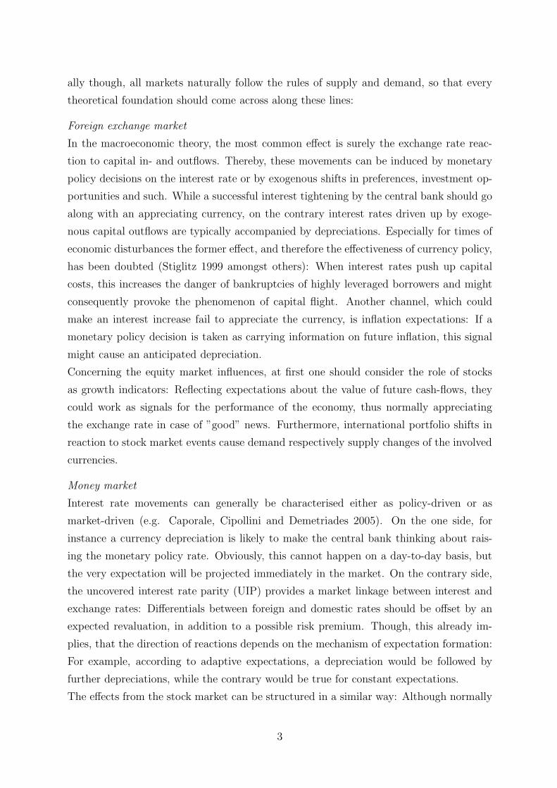
ally though, all markets naturally follow the rules of supply and demand, so that every
theoretical foundation should come across along these lines:
Foreign exchange market
In the macroeconomic theory, the most common effect is surely the exchange rate reac-
tion to capital in- and outflows. Thereby, these movements can be induced by monetary
policy decisions on the interest rate or by exogenous shifts in preferences, investment op-
portunities and such. While a successful interest tightening by the central bank should go
along with an appreciating currency, on the contrary interest rates driven up by exoge-
nous capital outflows are typically accompanied by depreciations. Especially for times of
economic disturbances the former effect, and therefore the effectiveness of currency policy,
has been doubted (Stiglitz 1999 amongst others): When interest rates push up capital
costs, this increases the danger of bankruptcies of highly leveraged borrowers and might
consequently provoke the phenomenon of capital flight. Another channel, which could
make an interest increase fail to appreciate the currency, is inflation expectations: If a
monetary policy decision is taken as carrying information on future inflation, this signal
might cause an anticipated depreciation.
Concerning the equity market influences, at first one should consider the role of stocks
as growth indicators: Reflecting expectations about the value of future cash-flows, they
could work as signals for the performance of the economy, thus normally appreciating
the exchange rate in case of ”good” news. Furthermore, international portfolio shifts in
reaction to stock market events cause demand respectively supply changes of the involved
currencies.
Money market
Interest rate movements can generally be characterised either as policy-driven or as
market-driven (e.g. Caporale, Cipollini and Demetriades 2005). On the one side, for
instance a currency depreciation is likely to make the central bank thinking about rais-
ing the monetary policy rate. Obviously, this cannot happen on a day-to-day basis, but
the very expectation will be projected immediately in the market. On the contrary side,
the uncovered interest rate parity (UIP) provides a market linkage between interest and
exchange rates: Differentials between foreign and domestic rates should be offset by an
expected revaluation, in addition to a possible risk premium. Though, this already im-
plies, that the direction of reactions depends on the mechanism of expectation formation:
For example, according to adaptive expectations, a depreciation would be followed by
further depreciations, while the contrary would be true for constant expectations.
The effects from the stock market can be structured in a similar way: Although normally
3
denied, equity developments have a signalling function for the monetary policy. Herein,
I consider the channels of changes in wealth respectively consumption, of corporate in-
vestment costs and again of growth indication (e.g. Rigobon and Sack 2003a). Another
mechanism probably works through the tendency of investors to switch to relatively safe
bonds or money market assets in times of economic difficulties.
Stock market
Impacts on the equity index naturally are propagated through the formation of expecta-
tions, but remain theoretically indefinite in their overall direction: Taking the example of
a currency depreciation, the fear of capital outflows and monetary tightening would have
a negative influence on the equity performance. Notwithstanding, hopes of strengthening
exports or rising retail prices would produce the contrary result. At last the concept of
UIP can as well be applied to equity returns (URP: ”uncovered equity return parity”, see
Cappiello and De Santis 2005), with the same decisive role of the form of expectations.
Theories on stock market reactions to interest rate movements have been worked out rela-
tively well (e.g. Andersen, Bollerslev, Diebold and Vega 2005). Straightforward channels
can be established by defining the stock price as the sum of discounted future cash-flows:
On the one hand, a negative impact comes through the interest rate reflecting opportu-
nity and investment costs. On the other hand, interest rates contain signals of future
economic growth, thereby raising expected profits hand in hand with the equity index. In
the literature, theoretical and empirical results seem to favour the view, that the former
effect dominates during economic upswings, while the latter, unfortunately in the reverse
direction, is more important in recessions (e.g. Andersen, Bollerslev, Diebold and Vega
2005 or Boyd, Hu and Jagannathan 2005). Of course, besides signals about growth, the
interest rate could as well carry information about future inflation, for example as in the
Fisher equation, and the course of monetary policy. The related impact is straightforward
as explained above.
Obviously, not all mentioned effects can be of the same importance in every country
model. In the particular context of post-crisis Asian-Pacific financial markets the focus
should be on the following points:
• Does monetary policy try to stabilise the currency?
• Can it succeed in this attempt?
• How important are exchange rate stability and interest rate movements for the
overall economic performance?
4

Volatility effects
Up to now, the argumentation has aimed at interrelations between the levels of the three
financial variables. In general, all these connections could as well be thought of in the
domain of variability, but here the theoretical foundation is rather poor. Nevertheless,
volatility transmission matters for monetary policy decisions, the construction of stable
financial systems, risk hedging or the reduction of vulnerability, amongst others. There-
fore, on this stage I present some stylised facts, which could possibly be found in the
empirical analysis:
• Concerning the exchange rate, one main question is, whether higher variability
is brought into an economy by foreign linkages. Might currency revaluations for
example cause speculations about central bank decisions, or does the stock market
show signs of increased activity?
• Put it the other way round, does monetary policy itself induce fluctuations, as it is
claimed by neoclassical theories?
• At last, in how far are contagion effects from the traditionally volatile stock market
existing?
3 Methodological Proceeding
3.1 Models for the Mean Process
The basic generating process of the data (here exchange rate, money market rate and
stock index) in the econometric procedure is assumed to be the structural-form VAR with
lag length q + 1
Ayt = µ∗0 + µ∗
1t + µ2dt +
q+1∑j=1
B∗j yt−j + εt , (1)
where yt contains the n (here 3) endogenous variables, B∗j are n×n coefficient matrices and
εt is an n-dimensional vector of uncorrelated heteroscedastic residuals. The deterministic
terms are a constant, a linear trend (t) and centred daily seasonal dummies (dt), which
control for possible day-of-the-week effects.
Given the presence of unit roots in the data, according to Johansen (1995), the common-
ness of n − r stochastic trends is reflected by a reduced rank of B∗(1), with B∗(L) =
A −∑q+1i=1 B∗
j Lj. Consequently, one can write B∗(1) = −αβ ′, where β spans the space
of the r cointegrating vectors, and α contains the corresponding adjustment coefficients.
5
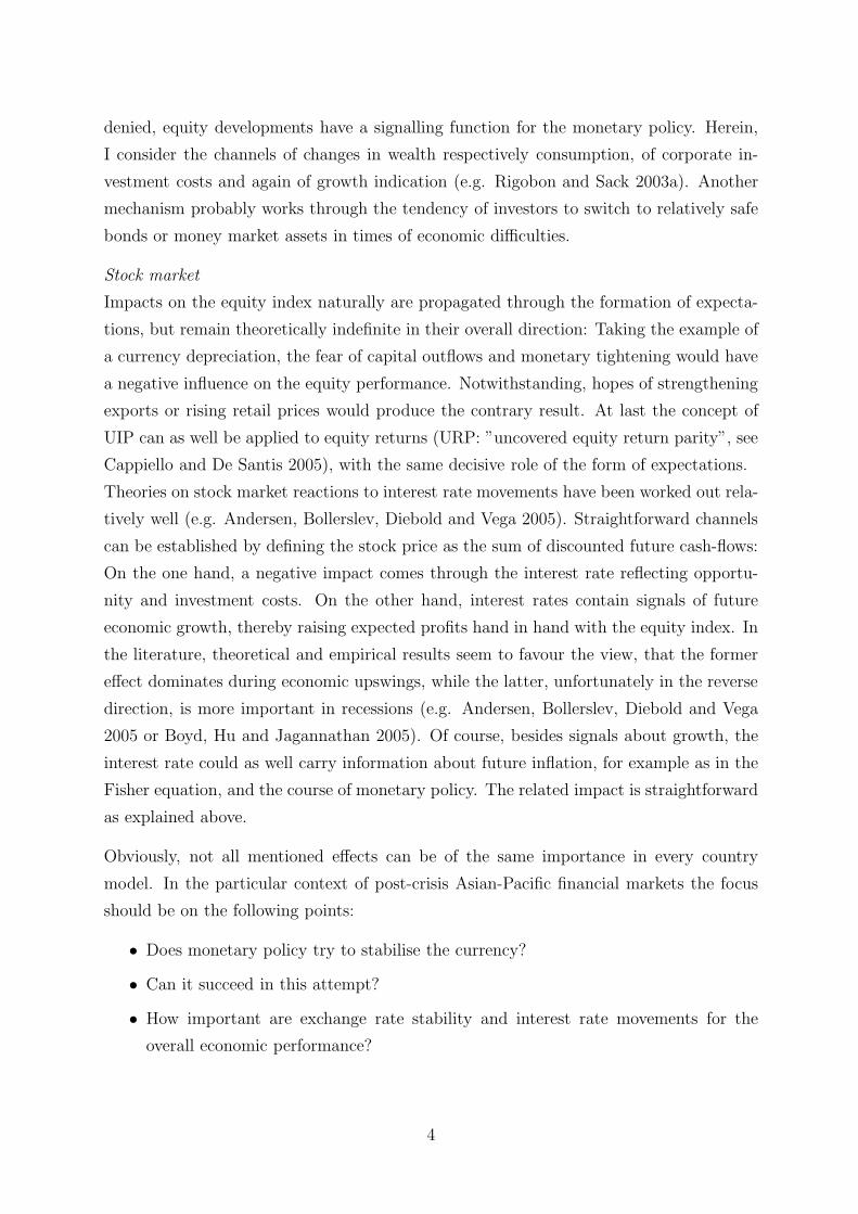
Granger’s representation theorem then leads to the structural VECM
A∆yt = α[β ′yt−1 + µ0 + µ1(t − 1)] + µ2dt +
q∑j=1
Bj∆yt−j + εt , (2)
with Bj = −∑q+1k=j+1 B∗
k, j = 1, . . . , q. Constant and trend are assumed to be absorbed
in the cointegrating relation.
Since (2) for itself is not identified, the reduced-form VECM is derived:
∆yt = αr[β ′yt−1 + µ0 + µ1(t − 1)] + µr2dt +
q∑j=1
Brj ∆yt−j + ut . (3)
All coefficients are obtained by premultiplying A−1 in (2), therefore being marked by the
superscript r for ”reduced”. Accordingly, the new residuals are given by ut = A−1εt.
The unit root behaviour of the series is checked by the standard ADF test (see e.g. Dickey
and Fuller 1979), including a constant, a trend and centred seasonal dummies. Here, as
well as in all subsequent models, the lag length is set following the usual information
criteria (maximum lag 10) and autocorrelation tests. Simulated critical values for the
null hypothesis of non-stationarity are taken from MacKinnon (1991, 1996).
For finding out the number of common stochastic trends, Johansen (1994, 1995) provides
the likelihood ratio trace test. The test statistic for the null hypothesis of at most r
cointegrating relations is given by:
Λ(r) = −T
n∑j=r+1
log(1 − λj) , (4)
where n is the number of endogenous variables and T the number of observations. λj de-
notes the j-th largest squared sample canonical correlation between ∆yt and the respective
cointegrating relation, both corrected for the influence of the remaining regressors. Crit-
ical values are obtained by computing the response surface in Doornik (1998).
In case even r = 0 is not rejected, equations (2) and (3) are specified without any cointe-
gration terms, simply leaving VARs in first differences. Consequently, constant and trend
are then considered outside the cointegrating relations.
3.2 Identification through Heteroscedasticity
In the structural VAR equation (1), the matrix A of contemporaneous effects cannot be
identified without further constraints. The theoretical considerations in section 2 found
6

reasons for various possible effects between all variables and therefore did not justify
any zero restrictions. By the same token, it proves impossible to recover the structural
parameters from the reduced form given by (2): In the matrix A with normalised diag-
onal, n(n − 1) simultaneous impacts have to be estimated, but due to its symmetry the
covariance-matrix of the reduced-form residuals delivers only n(n − 1)/2 equations for
simultaneous covariances.
In spite of reducing the number of parameters by restrictions, the present approach aims
on principle at augmenting the number of determining equations (see Rigobon 2003): If
one can identify for example several regimes with differing volatility, the necessary shifts in
the covariance-matrix yield additional equations for uncovering the structural parameters,
which for their part have to be assumed constant over time.
The next section describes the set-up and estimation of a so-called ”structural GARCH”
model. In this, I follow basically the intuition of identification through volatility regimes.
Estimating a multivariate GARCH however is equal to modelling a continuum of regimes,
which is reflected in the estimated variance processes.
3.3 Structural EGARCH
Since the variance model shall be specified for the structural residuals, according to (3),
these are recovered by
εt = Aut . (5)
Furthermore, define the conditional variances of the elements in εt by
Var(εjt|It−1) = Vart−1(εjt) = hjt j = 1, . . . , n , (6)
where It−1 denotes the whole set of available information at time t − 1. The conditional
covariances of the structural residuals are assumed to be zero, what is in analogy to the
standard identifying procedure.
Then, stack the hjt in the vector Ht =(
h1t h2t . . . hnt
)′.
At last, denote the standardised white noise residuals by
εjt = εjt/√
hjt j = 1, . . . , n . (7)
The multivariate EGARCH(1,1)-process is then given by
log Ht = C + G log Ht−1 + D|εt−1| + F εt−1 , (8)
7

where C is an n × 1 vector of constants, and G, D and F are n × n coefficient matrices.
The absolute value operation is to be applied element by element.
The univariate EGARCH has been proposed by Nelson (1991). With the conditional
covariances of the structural residuals assumed to be zero, the multivariate extension (8)
only comprises the conditional variances. By taking logarithms, the EGARCH model
guarantees these variances to be positive. Together with the zero correlations assump-
tion, this is sufficient for positive definite covariance matrices. Furthermore, asymmetric
effects are incorporated by including εt without taking absolute values: Any parame-
ters in F differing from zero indicate, that besides the magnitude of a shock its sign
contains valuable information for forecasting the conditional variances. EGARCH(1,1)
seems to be appropriate for most series, what will be shown by Lagrange Multiplier (LM)
GARCH-tests, has additionally been checked in univariate models and is quite usual in
financial econometrics. Apart from that, higher-order lags would considerably complicate
the likelihood optimisation.
Let Σt denote the conditional covariance-matrix of εt including the hjt on the main diag-
onal and zeros off-diagonal. Then the log-likelihood under the assumption of conditional
normality results as
L(A, C, G, D, F ) = L(θ) =T∑
t=1
log lt(θ) = −1
2
T∑t=1
(n log 2π + log |Σt| + ε′tεt) . (9)
Since assuming conditional normality is often problematic using financial markets data,
the estimation relies on Quasi-Maximum-Likelihood (Bollerslev and Wooldridge 1992).
While excess kurtosis may be taken as an argument for adopting in example a Student-t-
distribution, QML has the advantage of consistency even if the distributional assumption
is violated. Although consistency and asymptotic normality are not proven for my par-
ticular model, results from the MGARCH literature suggest, that
√T (θ − θ)
d→ N(0, M−11 M0M
−11 ) , (10)
where M1 = −E(∂2 log lt(θ)∂θ∂θ′ ) and M0 = E(∂ log lt(θ)
∂θ∂ log lt(θ)
∂θ′ ) (see Comte and Lieberman
2003). Note, that the usual ML covariance matrix estimator M−11 would not be consistent
under non-normality.
The likelihood optimisation is done using the BHHH algorithm (Berndt, Hall, Hall and
Hausman 1974) in the Gauss Maxlik procedure, the code is written by the author. The
parameter starting values are obtained from the univariate EGARCH estimates, the struc-
tural and cross-effect coefficients are set to zero, and the variance process is started at
8

the sample moments. The choice of the starting values did not prove crucial, supported
by the common result in the multivariate GARCH literature, that in any case most cross-
coefficients are insignificant.
3.4 Combining Reduced-Form and Structural Estimates
In the first two steps, the reduced form (3) and the structural EGARCH (8) have been
estimated. At last, the obtained A-matrix is substituted in equation (2), which is then re-
estimated to gain values and standard errors of the remaining parameters. This procedure
allows the determination of dynamic effects running over a certain time span in addition
to the contemporaneous impacts from the identified structural matrix.
In order to present a measure of the overall interaction between the variables, I compute
the matrix of total effects, which are reached after the adjustment processes have been
completely finished. For VARs in first differences, the long-run level impacts are given as
elements of
Ξ = (A −q∑
j=1
Bj)−1 . (11)
For the cointegrating models, the matrix can be derived from the VECM moving average
representation (Johansen 1995):
Ξ = β⊥(α′⊥(A −
q∑j=1
Bj)β⊥)−1α′⊥ , (12)
with ⊥ denoting the orthogonal complement (thus α′α⊥ = 0, where both α and α⊥ have
full column rank).
4 Empirical Evidence
4.1 Data
This study employs the common representative daily data for the foreign exchange, money
and stock markets: the exchange rates e measured in domestic currency units per US
dollar, the three-month money market rates i (short-term government bonds, where not
available) and the main national stock indices s. The money market rate at the short end
of the yield curve should be close enough to monetary policy decisions on the one hand,
9

but should at the same time exhibit sufficient continuous market-driven variation on the
other.
The sample from 01/04/1999 till 10/09/2006 covers the years since the Asian financial
crisis in 1997/98. The countries are Australia, Hong Kong (Special Administrative Region
of China), India, Indonesia, Japan, New Zealand, the Philippines, Singapore, South Korea
(”Korea” in the following), Taiwan and Thailand. The interesting cases of China and
Malaysia had to be left out, because their highly regulated interest and exchange rates
are not suitable for an application of time series techniques. Figure 1 gives an overview
of the time series; the three cases with shortened line graphs are due to scarce data
availability.
In the foreign exchange market, most currencies depreciated moderately against the US
dollar until 2001/2002, then appreciation sets in. For the interest rates, the same pat-
tern could be dismantled: Normally falling till about 2003, an upturn can be detected
afterwards. In the same period, the equity indices show clear signs of a stock exchange
rallying. Obviously, these developments are directed by the course of the business cycle:
Immediately after the crisis, the making up generated a growth peak, but the following re-
cession in the world economy did not spare the Asian Pacific region. Though, a profound
recovery seems to take place at the latest since 2003.
For the empirical analysis, the exchange rates and the stock indices are transformed
to logarithms multiplied by 100. Then, taking first differences generates continuously
compounded asset returns or growth rates in percentage points. As the interest rates are
already measured in percentage points and normally remain rather low, no transformation
is applied. Nonetheless, it is necessary to proceed with care in the parameter interpreta-
tion: For example, a rise of one in an annualised interest rate is equal to four standard
discount rate steps of a central bank, which would be a tremendous change in contrast to
a daily stock return of one percent.
Tackling the degree of persistence in the data, Table 1 displays the p-values of the ADF-
tests on the chosen series E, I and S, where the former and the latter are in logs as
told above. The hypotheses of non-stationarity are confirmed, and additionally, the first
differences are clearly I(0). Solely the unit root results for the Philippine interest rate are
unclear, even through several tests. I will treat it conformable as an I(1)-variable, therefore
naturally running the risk of over-differencing, but avoiding unbalanced regressions. The
calculations in this paper have been done in Gauss 8.0, JMulti 4.14 and EViews 5.0.
10

1.2
1.3
1.4
1.5
1.6
1.7
1.8
1.9
2.0
2.1
1999 2000 2001 2002 2003 2004 2005 2006
AUS_E
4.0
4.5
5.0
5.5
6.0
6.5
7.0
1999 2000 2001 2002 2003 2004 2005 2006
AUS_I
2500
3000
3500
4000
4500
5000
5500
1999 2000 2001 2002 2003 2004 2005 2006
AUS_S
7.70
7.72
7.74
7.76
7.78
7.80
7.82
1999 2000 2001 2002 2003 2004 2005 2006
HK_E
0
1
2
3
4
5
6
7
8
1999 2000 2001 2002 2003 2004 2005 2006
HK_I
8000
10000
12000
14000
16000
18000
20000
1999 2000 2001 2002 2003 2004 2005 2006
HK_S
8000
8500
9000
9500
10000
10500
11000
1999 2000 2001 2002 2003 2004 2005 2006
I DN_E
6
8
10
12
14
16
1999 2000 2001 2002 2003 2004 2005 2006
I DN_I
400
600
800
1000
1200
1400
1600
1999 2000 2001 2002 2003 2004 2005 2006
I DN_S
42
43
44
45
46
47
48
49
50
1999 2000 2001 2002 2003 2004 2005 2006
I NDI A_E
4
5
6
7
8
9
10
11
12
13
1999 2000 2001 2002 2003 2004 2005 2006
I NDI A_I
1000
2000
3000
4000
5000
6000
7000
1999 2000 2001 2002 2003 2004 2005 2006
I NDI A_S
100
105
110
115
120
125
130
135
1999 2000 2001 2002 2003 2004 2005 2006
JPN_E
.0
.1
.2
.3
.4
.5
.6
.7
.8
1999 2000 2001 2002 2003 2004 2005 2006
JPN_I
6000
8000
10000
12000
14000
16000
18000
20000
22000
1999 2000 2001 2002 2003 2004 2005 2006
JPN_S
900
1000
1100
1200
1300
1400
1999 2000 2001 2002 2003 2004 2005 2006
KOR_E
3
4
5
6
7
8
9
10
1999 2000 2001 2002 2003 2004 2005 2006
KOR_I
400
600
800
1000
1200
1400
1600
1999 2000 2001 2002 2003 2004 2005 2006
KOR_S
11

1.2
1.4
1.6
1.8
2.0
2.2
2.4
2.6
1999 2000 2001 2002 2003 2004 2005 2006
NZL_E
3
4
5
6
7
8
1999 2000 2001 2002 2003 2004 2005 2006
NZL_I
600
700
800
900
1000
1100
1200
1999 2000 2001 2002 2003 2004 2005 2006
NZL_S
36
40
44
48
52
56
60
1999 2000 2001 2002 2003 2004 2005 2006
PLP_E
0
5
10
15
20
25
30
35
1999 2000 2001 2002 2003 2004 2005 2006
PLP_I
400
600
800
1000
1200
1400
1600
1999 2000 2001 2002 2003 2004 2005 2006
PLP_S
1.56
1.60
1.64
1.68
1.72
1.76
1.80
1.84
1.88
1999 2000 2001 2002 2003 2004 2005 2006
SGP_E
0.4
0.8
1.2
1.6
2.0
2.4
2.8
3.2
3.6
1999 2000 2001 2002 2003 2004 2005 2006
SGP_I
300
400
500
600
700
1999 2000 2001 2002 2003 2004 2005 2006
SGP_S
37
38
39
40
41
42
43
44
45
46
1999 2000 2001 2002 2003 2004 2005 2006
THL_E
1
2
3
4
5
6
1999 2000 2001 2002 2003 2004 2005 2006
THL_I
200
300
400
500
600
700
800
1999 2000 2001 2002 2003 2004 2005 2006
THL_S
30
31
32
33
34
35
36
1999 2000 2001 2002 2003 2004 2005 2006
TW N_E
1
2
3
4
5
6
7
1999 2000 2001 2002 2003 2004 2005 2006
TW N_I
3000
4000
5000
6000
7000
8000
9000
10000
11000
1999 2000 2001 2002 2003 2004 2005 2006
TW N_S
Figure 1: Exchange rates (E), money market rates (I) and stock indices (S)
12

AUS HK IDN INDIA JPN KOR NZL PLP SGP THL TWN
E 0.79 0.20 0.44 0.78 0.55 0.83 0.71 0.97 0.46 0.06 0.86[lags] 0 0 0 0 0 1 0 0 0 0 1
I 0.82 0.73 0.56 0.53 0.61 0.71 0.92 0.01 0.84 0.96 0.64[lags] 2 1 0 0 1 1 0 8 0 3 3
S 0.89 0.83 0.93 0.94 0.96 0.66 0.52 0.82 0.91 0.76 0.78[lags] 0 0 1 1 0 0 0 1 0 0 0
Deterministics: constant, linear trend in E and S when significant
Table 1: p-values of ADF-tests
4.2 Specification of the Reduced-Form Models
In order to find acceptable specifications of the reduced-form VECM in (3), the numbers
of lags and of cointegrating relations have to be determined. The former are chosen by
the usual information criteria and are checked by LM tests (see Doornik 1996) with the
null hypothesis of no autocorrelation, see Table 2. While the overall impression is quite
satisfying, several rejections appear especially for the higher order. Nevertheless, for the
most part of the variables, the serial correlation should be completely captured.
AUS HK IDN INDIA JPN KOR NZL PLP SGP THL TWN
LM(1) 0.09 0.04 0.72 0.75 0.33 0.17 0.37 0.31 0.03 0.83 0.88
LM(5) 0.28 0.13 0.35 0.01 0.11 0.00 0.02 0.00 0.02 0.17 0.60
lags 2 2 5 1 3 1 1 2 1 3 5
Table 2: p-values of LM-tests for no residual autocorrelation
Concerning the cointegration properties, Table 3 shows the p-values for the trace tests
between the interest rates and the stock indices in bivariate models. Here, the exchange
rates are not considered, because UIP or URP theoretically rule out any cointegrating
relations, what has also been confirmed empirically in the run-up. Consequently, one
common stochastic trend (plus the exchange rate trend in the trivariate system) is ac-
cepted for Japan, Korea and New Zealand. It is true, that the former does not yield clear
significance, but the resulting VECM proved very robust and sensible, contrasting for
example with a similar model for Taiwan. The low p-value for the Philippines is strictly
due to the possible stationarity of its money market rate, therefore giving no grounds to
specify a cointegration model.
13

AUS HK IDN INDIA JPN KOR NZL PLP SGP THL TWN
H0 : r = 0 0.81 0.74 0.35 0.60 0.13∗ 0.00∗ 0.06∗ 0.02 0.16 0.57 0.14
* H0 (no cointegration) rejected
Deterministics: constant, linear trend when significant
Table 3: p-values of trace tests for cointegration between i and s
4.3 Financial Volatility Transmission
While the reduced-form models have already been specified, the structural VARs and
VECMs can only be estimated in the last step after the identification of the contempo-
raneous impact matrix. Therefore, at first the results for the generating processes of the
conditional variances shall be presented, grouped by several similarities among certain
models. Naturally, there are no cases with insignificant parameters on the diagonals of
the first two matrices, thus showing the pure presence of ARCH effects in the data. The
QML standard errors are put in parentheses below the coefficients.
The most simple variance equations arise from the estimations for Australia, Korea and
Taiwan. Here, all non-diagonal elements are clearly insignificant, ruling out any causality
in variance between the different variables. The only asymmetry appears as the well-
known leverage effect in the stock market, which can be found in nearly all models: The
negative coefficients indicate, that negative shocks to equity prices have higher volatility
impacts than positive ones.
Australia
⎛⎜⎝
log het
log hit
log hst
⎞⎟⎠=
⎛⎜⎜⎜⎜⎜⎜⎝
−0.050(0.009)
−0.395(0.179)
−0.122(0.030)
⎞⎟⎟⎟⎟⎟⎟⎠+
⎛⎜⎜⎜⎜⎜⎜⎝
0.994 0 0(0.003)
0 0.976 0(0.016)
0 0 0.976(0.009)
⎞⎟⎟⎟⎟⎟⎟⎠
⎛⎜⎝
log het−1
log hit−1
log hst−1
⎞⎟⎠+
⎛⎜⎜⎜⎜⎜⎜⎝
0.057 0 0(0.011)
0 0.324 0(0.108)
0 0 0.135(0.034)
⎞⎟⎟⎟⎟⎟⎟⎠
⎛⎜⎝|εet−1||εit−1||εst−1|
⎞⎟⎠+
⎛⎜⎜⎜⎜⎜⎜⎝
0 0 0
0 0 0
0 0 −0.094(0.024)
⎞⎟⎟⎟⎟⎟⎟⎠
⎛⎜⎝
εet−1
εit−1
εst−1
⎞⎟⎠
Korea
⎛⎜⎝
log het
log hit
log hst
⎞⎟⎠=
⎛⎜⎜⎜⎜⎜⎜⎝
−0.169(0.032)
−0.515(0.304)
−0.067(0.023)
⎞⎟⎟⎟⎟⎟⎟⎠+
⎛⎜⎜⎜⎜⎜⎜⎝
0.969 0 0(0.012)
0 0.943 0(0.039)
0 0 0.992(0.007)
⎞⎟⎟⎟⎟⎟⎟⎠
⎛⎜⎝
log het−1
log hit−1
log hst−1
⎞⎟⎠+
⎛⎜⎜⎜⎜⎜⎜⎝
0.157 0 0(0.027)
0 0.273 0(0.121)
0 0 0.102(0.040)
⎞⎟⎟⎟⎟⎟⎟⎠
⎛⎜⎝|εet−1||εit−1||εst−1|
⎞⎟⎠+
⎛⎜⎜⎜⎜⎜⎜⎝
0 0 0
0 0 0
0 0 −0.038(0.020)
⎞⎟⎟⎟⎟⎟⎟⎠
⎛⎜⎝
εet−1
εit−1
εst−1
⎞⎟⎠
Taiwan
⎛⎜⎝
log het
log hit
log hst
⎞⎟⎠=
⎛⎜⎜⎜⎜⎜⎜⎝
−0.238(0.117)
−0.204(0.045)
−0.084(0.019)
⎞⎟⎟⎟⎟⎟⎟⎠+
⎛⎜⎜⎜⎜⎜⎜⎝
0.959 0 0(0.041)
0 0.986 0(0.005)
0 0 0.986(0.007)
⎞⎟⎟⎟⎟⎟⎟⎠
⎛⎜⎝
log het−1
log hit−1
log hst−1
⎞⎟⎠+
⎛⎜⎜⎜⎜⎜⎜⎝
0.197 0 0(0.048)
0 0.212 0(0.027)
0 0 0.126(0.031)
⎞⎟⎟⎟⎟⎟⎟⎠
⎛⎜⎝|εet−1||εit−1||εst−1|
⎞⎟⎠+
⎛⎜⎜⎜⎜⎜⎜⎝
0 0 0
0 0 0
0 0 −0.056(0.018)
⎞⎟⎟⎟⎟⎟⎟⎠
⎛⎜⎝
εet−1
εit−1
εst−1
⎞⎟⎠
14
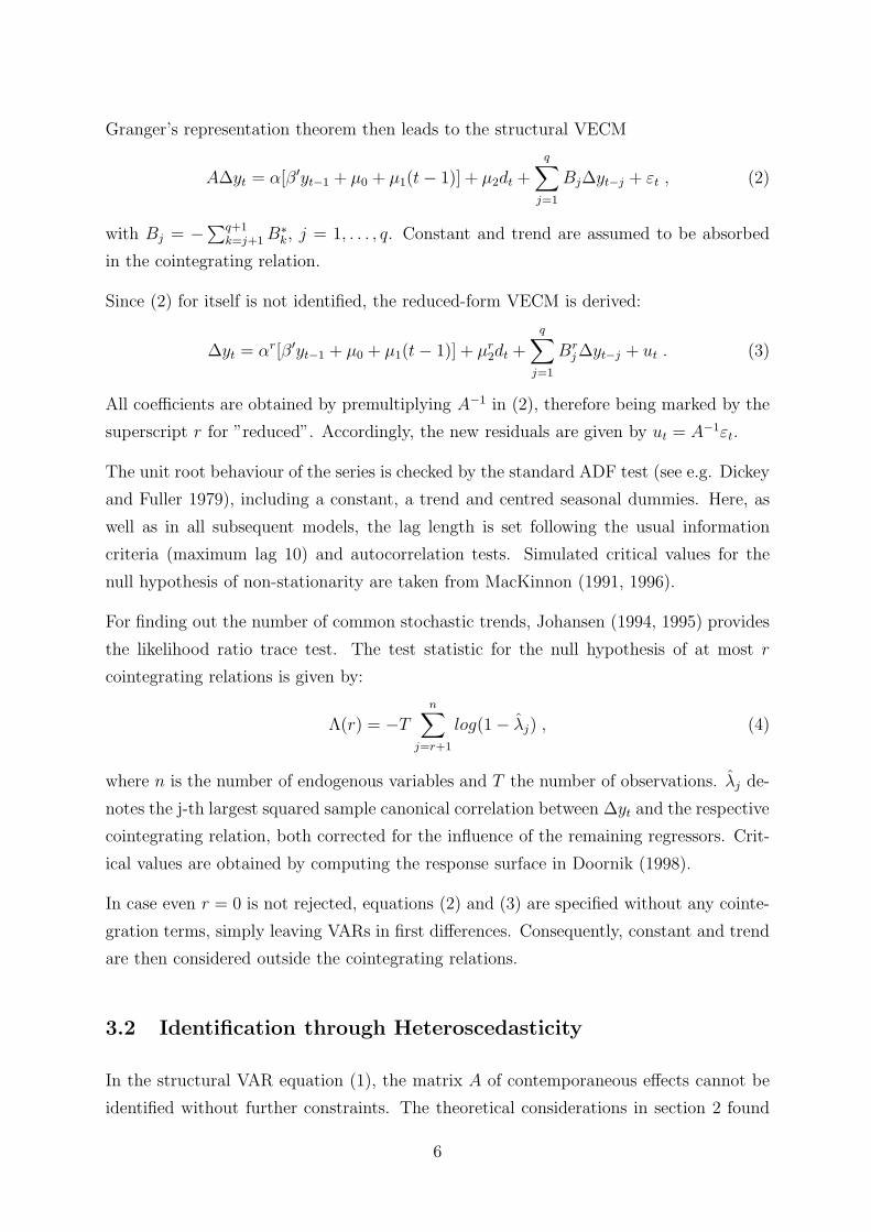
One cross-effect each can be found for New Zealand and Singapore: In New Zealand,
exchange rate shocks have a considerable impact on the money market variance, what
could be seen as typical for a small open economy. In Singapore, equity price shocks
prove relevant for the foreign exchange market, probably explained by the role of the city
state as an Asian financial centre.
New Zealand
⎛⎜⎝
log het
log hit
log hst
⎞⎟⎠=
⎛⎜⎜⎜⎜⎜⎜⎝
−0.043(0.012)
−0.663(0.227)
−0.119(0.032)
⎞⎟⎟⎟⎟⎟⎟⎠+
⎛⎜⎜⎜⎜⎜⎜⎝
0.994 0 0(0.009)
0 0.947 0(0.026)
0 0 0.979(0.009)
⎞⎟⎟⎟⎟⎟⎟⎠
⎛⎜⎝
log het−1
log hit−1
log hst−1
⎞⎟⎠+
⎛⎜⎜⎜⎜⎜⎜⎝
0.052 0 0(0.015)
0.174 0.226 0(0.067) (0.074)
0 0 0.135(0.036)
⎞⎟⎟⎟⎟⎟⎟⎠
⎛⎜⎝|εet−1||εit−1||εst−1|
⎞⎟⎠+
⎛⎜⎜⎜⎜⎜⎜⎝
0 0 0
0 0 0
0 0 −0.040(0.017)
⎞⎟⎟⎟⎟⎟⎟⎠
⎛⎜⎝
εet−1
εit−1
εst−1
⎞⎟⎠
Singapore
⎛⎜⎝
log het
log hit
log hst
⎞⎟⎠=
⎛⎜⎜⎜⎜⎜⎜⎝
−0.298(0.084)
−0.284(0.065)
−0.129(0.024)
⎞⎟⎟⎟⎟⎟⎟⎠+
⎛⎜⎜⎜⎜⎜⎜⎝
0.939 0 0(0.023)
0 0.976 0(0.007)
0 0 0.990(0.007)
⎞⎟⎟⎟⎟⎟⎟⎠
⎛⎜⎝
log het−1
log hit−1
log hst−1
⎞⎟⎠+
⎛⎜⎜⎜⎜⎜⎜⎝
0.094 0 0.088(0.028) (0.042)
0 0.201 0(0.040)
0 0 0.170(0.032)
⎞⎟⎟⎟⎟⎟⎟⎠
⎛⎜⎝|εet−1||εit−1||εst−1|
⎞⎟⎠+
⎛⎜⎜⎜⎜⎜⎜⎝
0 0 0
0 0 0
0 0 −0.031(0.013)
⎞⎟⎟⎟⎟⎟⎟⎠
⎛⎜⎝
εet−1
εit−1
εst−1
⎞⎟⎠
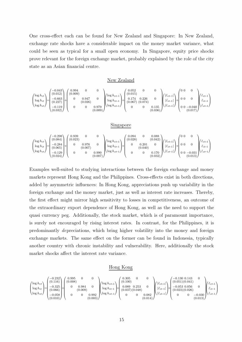
Examples well-suited to studying interactions between the foreign exchange and money
markets represent Hong Kong and the Philippines. Cross-effects exist in both directions,
added by asymmetric influences: In Hong Kong, appreciations push up variability in the
foreign exchange and the money market, just as well as interest rate increases. Thereby,
the first effect might mirror high sensitivity to losses in competitiveness, an outcome of
the extraordinary export dependence of Hong Kong, as well as the need to support the
quasi currency peg. Additionally, the stock market, which is of paramount importance,
is surely not encouraged by rising interest rates. In contrast, for the Philippines, it is
predominantly depreciations, which bring higher volatility into the money and foreign
exchange markets. The same effect on the former can be found in Indonesia, typically
another country with chronic instability and vulnerability. Here, additionally the stock
market shocks affect the interest rate variance.
Hong Kong
⎛⎜⎝
log het
log hit
log hst
⎞⎟⎠=
⎛⎜⎜⎜⎜⎜⎜⎝
−0.232(0.116)
−0.325(0.066)
−0.058(0.010)
⎞⎟⎟⎟⎟⎟⎟⎠+
⎛⎜⎜⎜⎜⎜⎜⎝
0.995 0 0(0.008)
0 0.984 0(0.009)
0 0 0.992(0.003)
⎞⎟⎟⎟⎟⎟⎟⎠
⎛⎜⎝
log het−1
log hit−1
log hst−1
⎞⎟⎠+
⎛⎜⎜⎜⎜⎜⎜⎝
0.305 0 0(0.100)
0.089 0.253 0(0.037)(0.048)
0 0 0.082(0.014)
⎞⎟⎟⎟⎟⎟⎟⎠
⎛⎜⎝|εet−1||εit−1||εst−1|
⎞⎟⎠+
⎛⎜⎜⎜⎜⎜⎜⎝
−0.130 0.143 0(0.051)(0.041)
−0.053 0.056 0(0.023)(0.026)
0 0 −0.030(0.013)
⎞⎟⎟⎟⎟⎟⎟⎠
⎛⎜⎝
εet−1
εit−1
εst−1
⎞⎟⎠
15

Philippines
⎛⎜⎝
log het
log hit
log hst
⎞⎟⎠=
⎛⎜⎜⎜⎜⎜⎜⎝
−0.341(0.057)
−0.542(0.074)
−0.137(0.032)
⎞⎟⎟⎟⎟⎟⎟⎠+
⎛⎜⎜⎜⎜⎜⎜⎝
0.982 0 0(0.010)
0 0.962 0(0.010)
0 0 0.944(0.024)
⎞⎟⎟⎟⎟⎟⎟⎠
⎛⎜⎝
log het−1
log hit−1
log hst−1
⎞⎟⎠+
⎛⎜⎜⎜⎜⎜⎜⎝
0.303 0.118 0(0.052)(0.046)
0.180 0.417 0(0.053)(0.059)
0 0 0.184(0.044)
⎞⎟⎟⎟⎟⎟⎟⎠
⎛⎜⎝|εet−1||εit−1||εst−1|
⎞⎟⎠+
⎛⎜⎜⎜⎜⎜⎜⎝
0.066 0 0.066(0.022) (0.028)
0.089 0.116 0(0.028)(0.034)
0 0 0
⎞⎟⎟⎟⎟⎟⎟⎠
⎛⎜⎝
εet−1
εit−1
εst−1
⎞⎟⎠
Indonesia
⎛⎜⎝
log het
log hit
log hst
⎞⎟⎠=
⎛⎜⎜⎜⎜⎜⎜⎝
−0.754(0.125)
−1.104(0.294)
−0.166(0.079)
⎞⎟⎟⎟⎟⎟⎟⎠+
⎛⎜⎜⎜⎜⎜⎜⎝
0.718 0 0(0.071)
0 0.850 0(0.050)
0 0 0.794(0.078)
⎞⎟⎟⎟⎟⎟⎟⎠
⎛⎜⎝
log het−1
log hit−1
log hst−1
⎞⎟⎠+
⎛⎜⎜⎜⎜⎜⎜⎝
0.418 0 0(0.072)
0 0.262 0.460(0.080)(0.206)
0 0 0.262(0.110)
⎞⎟⎟⎟⎟⎟⎟⎠
⎛⎜⎝|εet−1||εit−1||εst−1|
⎞⎟⎠+
⎛⎜⎜⎜⎜⎜⎜⎝
0 0 0
0.139 0 0(0.073)
0 0−0.172(0.076)
⎞⎟⎟⎟⎟⎟⎟⎠
⎛⎜⎝
εet−1
εit−1
εst−1
⎞⎟⎠
In India, falling equity prices raise the variability in the stock and foreign exchange mar-
kets. In turn, the stock index reacts to depreciating shocks, and in the money market,
above all contractionary shocks drive its variance. All in all, Indian markets seem to
be sensitive to reductions in the value of the respective assets. The Japanese estimated
cross-effects might be interpreted against the background of the deflationary period: Pos-
itive equity shocks serve as growth signals, giving grounds to deviate from the lasting
zero interest rate policy, interest rate increases reassure the foreign exchange market, and
exchange rate shocks matter for stock volatility.
India
⎛⎜⎝
log het
log hit
log hst
⎞⎟⎠=
⎛⎜⎜⎜⎜⎜⎜⎝
−0.391(0.108)
−0.204(0.095)
−0.139(0.023)
⎞⎟⎟⎟⎟⎟⎟⎠+
⎛⎜⎜⎜⎜⎜⎜⎝
0.966 0 0(0.016)
0 0.988 0(0.011)
0 0 0.925(0.020)
⎞⎟⎟⎟⎟⎟⎟⎠
⎛⎜⎝
log het−1
log hit−1
log hst−1
⎞⎟⎠+
⎛⎜⎜⎜⎜⎜⎜⎝
0.376 0 0(0.071)
0 0.208 0(0.067)
0 0 0.263(0.036)
⎞⎟⎟⎟⎟⎟⎟⎠
⎛⎜⎝|εet−1||εit−1||εst−1|
⎞⎟⎠+
⎛⎜⎜⎜⎜⎜⎜⎝
0 0 −0.060(0.026)
0 0.051 0(0.021)
0.084 0 −0.111(0.026) (0.027)
⎞⎟⎟⎟⎟⎟⎟⎠
⎛⎜⎝
εet−1
εit−1
εst−1
⎞⎟⎠
Japan
⎛⎜⎝
log het
log hit
log hst
⎞⎟⎠=
⎛⎜⎜⎜⎜⎜⎜⎝
−0.062(0.020)
−0.385(0.095)
−0.132(0.023)
⎞⎟⎟⎟⎟⎟⎟⎠+
⎛⎜⎜⎜⎜⎜⎜⎝
0.982 0 0(0.009)
0 0.986 0(0.008)
0 0 0.971(0.009)
⎞⎟⎟⎟⎟⎟⎟⎠
⎛⎜⎝
log het−1
log hit−1
log hst−1
⎞⎟⎠+
⎛⎜⎜⎜⎜⎜⎜⎝
0.056 0 0(0.018)
0 0.344 0(0.051)
0.063 0 0.130(0.026) (0.025)
⎞⎟⎟⎟⎟⎟⎟⎠
⎛⎜⎝|εet−1||εit−1||εst−1|
⎞⎟⎠+
⎛⎜⎜⎜⎜⎜⎜⎝
0−0.010 0(0.005)
0 0 0.121(0.042)
0 0 −0.053(0.018)
⎞⎟⎟⎟⎟⎟⎟⎠
⎛⎜⎝
εet−1
εit−1
εst−1
⎞⎟⎠
Thailand represents the only case with off-diagonal GARCH-parameters. On the one
hand, variance impacts from interest rate shocks in the foreign exchange market and from
the exchange rate on the equity index can be detected. On the other hand though, the
corresponding autoregressive coefficients are negative, so that the effect cushions very fast
in the following periods. Concerning the asymmetries, as in Hong Kong, again the strong
export orientation might be responsible for appreciations and bad equity news heightening
the exchange rate variability, which is anyway highly involved in the cross-dependences.
16

Thailand
⎛⎜⎝
log het
log hit
log hst
⎞⎟⎠=
⎛⎜⎜⎜⎜⎜⎜⎝
−0.439(0.077)
−0.809(0.201)
−0.206(0.040)
⎞⎟⎟⎟⎟⎟⎟⎠+
⎛⎜⎜⎜⎜⎜⎜⎝
0.981 −0.019 0(0.009) (0.006)
0 0.963 0(0.016)
−0.019 0 0.960(0.009) (0.010)
⎞⎟⎟⎟⎟⎟⎟⎠
⎛⎜⎝
log het−1
log hit−1
log hst−1
⎞⎟⎠+
⎛⎜⎜⎜⎜⎜⎜⎝
0.224 0.138 0(0.042) (0.043)
0.318 0.479 0(0.077) (0.147)
0.098 0 0.132(0.029) (0.031)
⎞⎟⎟⎟⎟⎟⎟⎠
⎛⎜⎝|εet−1||εit−1||εst−1|
⎞⎟⎠+
⎛⎜⎜⎜⎜⎜⎜⎝
−0.027 0 −0.033(0.014) (0.016)
0 0 0
0 −0.034 0(0.015)
⎞⎟⎟⎟⎟⎟⎟⎠
⎛⎜⎝
εet−1
εit−1
εst−1
⎞⎟⎠
Table 4 summarises the cross-effects in variance between the different financial markets.
As a first result, volatility transmission seems to appear above all in developing countries.
In general, this fact can be interpreted as both source and outcome of relatively higher
instability and insecurity in these economies. Recalling the initial main questions from
section 2, at first I can state, that the exchange rate indeed brings variability into the
domestic economy, above all into the money market. Monetary policy induced contagion
effects can be found in the exchange rate, but almost not in the stock index. In turn,
fluctuations from the equity prices spill over mainly into the foreign exchange market.
Effect Countries
exchange rate → interest rate NZL HK+ PLP− IDN− THL
exchange rate → stock index INDIA− JPN THL
interest rate → exchange rate HK+ PLP JPN− THL
interest rate → stock index THL−stock index → exchange rate SGP PLP+ INDIA− THL−stock index → interest rate IDN JPN+
+/− : Direction of asymmetry2
Table 4: Variance cross-effects in different countries
After presenting the results of the multivariate EGARCH estimations, I examine, if the
models catch up sufficiently the heteroscedasticity in the data. The p-values for the
ARCH-LM null hypothesis of no remaining ARCH in the residuals in Table 5 confirm the
standard literature result, that GARCH models of orders 1,1 are appropriate for financial
markets data. Given the quite considerable number of tests, several rejections should
not be too problematic. Furthermore, the autoregressive parameters smaller than one
meet the stability criterion; the still high persistence is a common feature throughout the
ARCH literature.
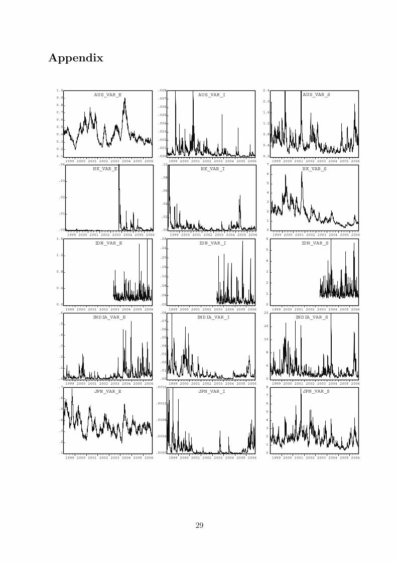
The graphs of the estimated conditional variances can be found in the Appendix Figure
2. As an overall impression, the volatilities in the money and stock markets might be
2The signs for the exchange rate appear reversed, because logically a depreciation is a negative change
despite the definition ”domestic currency / USD”.
17

AUS HK IDN INDIA JPN KOR NZL PLP SGP THL TWN
E 0.16 0.00 0.79 0.53 0.61 0.23 0.93 0.63 0.12 0.44 0.22LM(1) I 0.84 0.21 0.42 0.00 0.96 0.96 0.90 0.89 0.12 0.93 0.71
S 0.00 0.05 0.62 0.84 0.01 0.48 0.75 0.72 0.96 0.36 0.21
E 0.27 0.00 0.97 0.82 0.60 0.73 0.03 0.76 0.39 0.61 0.85LM(5) I 0.95 0.72 0.00 0.00 0.99 1.00 0.20 0.09 0.00 0.54 1.00
S 0.03 0.08 0.62 0.44 0.01 0.47 0.49 0.86 0.25 0.11 0.22
Table 5: p-values of LM-tests for no residual ARCH
slightly diminishing through time. While an economic stabilisation thus becomes evident,
no such clear pattern is revealed by the exchange rate variabilities.
4.4 Financial Markets Interlinkages
As has already been announced, this section contains the estimations of the fundamental
connections between the underlying financial markets. By maximising the likelihood
function (9), besides the EGARCH parameters, estimates of the contemporaneous impacts
are obtained. In the following VAR and VECM systems, the corresponding A matrices are
treated as given, what therefore allows the estimation of the right-hand sides of equation
(2), including as well the cointegrating relations. The dots serve as placeholders for the
deterministics and residuals. As a summary measure, below the respective equations, I
provide the total effects Ξ in the different models, which are usually reached quite quickly
in financial markets.
The long-run reactions of the variables to their own structural disturbances normally lie
around one. Only in the three models with cointegration (Japan, Korea, New Zealand)
the middle element is near or equal to zero, because the interest rate adjusts to the long-
run relation and therefore equalises all equilibrium deviations, including those produced
by its own shocks. Evidently, the interest rate is then bound to follow the development of
the overall economic performance revealed in the equity index. In the cases of Japan and
New Zealand, the interest rates even have zero total impact on all variables, since they
are the only ones adjusting to the cointegrating term. Above all, the stock prices are not
influenced by long-run disequilibria, thereby supporting the efficient market hypothesis.
For the better part of cases, the reactions of the exchange rates to money and stock
market shocks are straightforward: Increasing interest rates strengthen the currency, what
represents the textbook effect of monetary policy. Japan and New Zealand, for which the
18
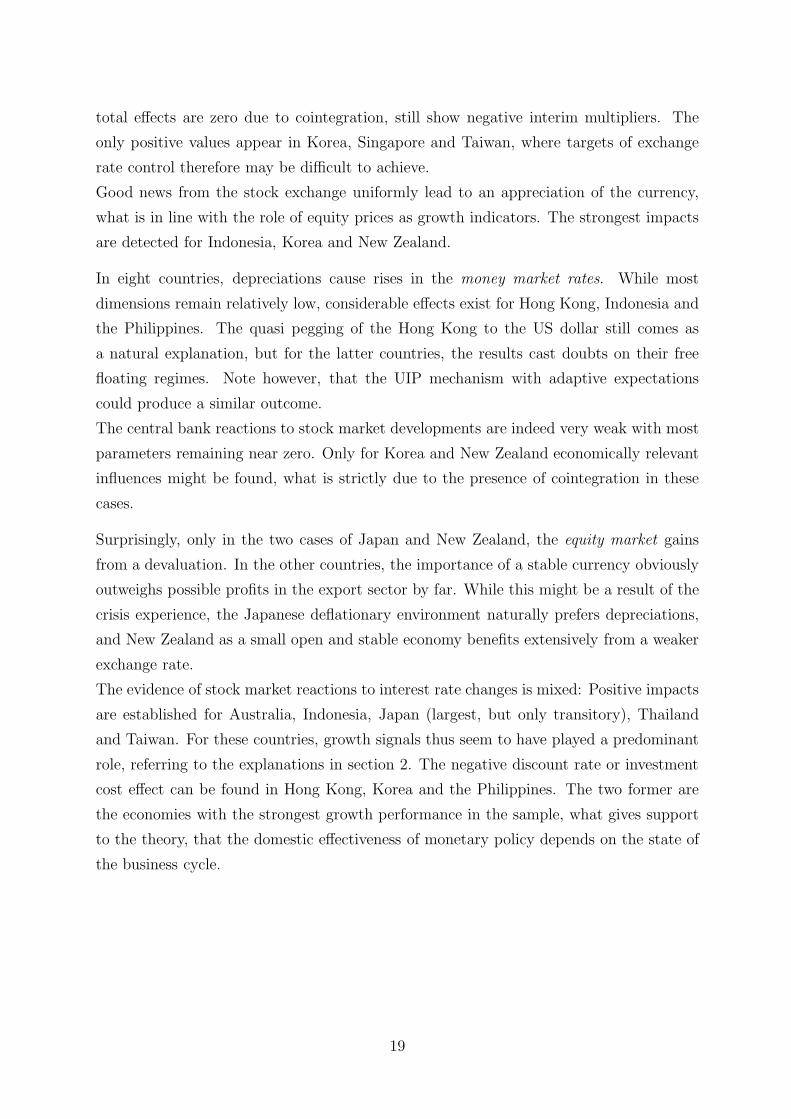
total effects are zero due to cointegration, still show negative interim multipliers. The
only positive values appear in Korea, Singapore and Taiwan, where targets of exchange
rate control therefore may be difficult to achieve.
Good news from the stock exchange uniformly lead to an appreciation of the currency,
what is in line with the role of equity prices as growth indicators. The strongest impacts
are detected for Indonesia, Korea and New Zealand.
In eight countries, depreciations cause rises in the money market rates. While most
dimensions remain relatively low, considerable effects exist for Hong Kong, Indonesia and
the Philippines. The quasi pegging of the Hong Kong to the US dollar still comes as
a natural explanation, but for the latter countries, the results cast doubts on their free
floating regimes. Note however, that the UIP mechanism with adaptive expectations
could produce a similar outcome.
The central bank reactions to stock market developments are indeed very weak with most
parameters remaining near zero. Only for Korea and New Zealand economically relevant
influences might be found, what is strictly due to the presence of cointegration in these
cases.
Surprisingly, only in the two cases of Japan and New Zealand, the equity market gains
from a devaluation. In the other countries, the importance of a stable currency obviously
outweighs possible profits in the export sector by far. While this might be a result of the
crisis experience, the Japanese deflationary environment naturally prefers depreciations,
and New Zealand as a small open and stable economy benefits extensively from a weaker
exchange rate.
The evidence of stock market reactions to interest rate changes is mixed: Positive impacts
are established for Australia, Indonesia, Japan (largest, but only transitory), Thailand
and Taiwan. For these countries, growth signals thus seem to have played a predominant
role, referring to the explanations in section 2. The negative discount rate or investment
cost effect can be found in Hong Kong, Korea and the Philippines. The two former are
the economies with the strongest growth performance in the sample, what gives support
to the theory, that the domestic effectiveness of monetary policy depends on the state of
the business cycle.
19

Australia
⎛⎜⎜⎜⎜⎜⎜⎝
1 0 0.085(0.021)
0 1 0
0.081 0 1(0.021)
⎞⎟⎟⎟⎟⎟⎟⎠
⎛⎜⎝
∆et
∆it
∆st
⎞⎟⎠=
⎛⎜⎜⎜⎜⎜⎜⎝
0 0 −0.073(0.020)
0 0.116 0(0.022)
0 0 −0.065(0.022)
⎞⎟⎟⎟⎟⎟⎟⎠
⎛⎜⎝
∆et−1
∆it−1
∆st−1
⎞⎟⎠+
⎛⎜⎜⎜⎜⎜⎜⎝
0 −1.939 0(0.640)
0 0.071 0.002(0.022) (0.001)
0 0 0
⎞⎟⎟⎟⎟⎟⎟⎠
⎛⎜⎝
∆et−2
∆it−2
∆st−2
⎞⎟⎠+. . .
Ξ =
⎛⎜⎝
1.013 −2.415 −0.155
−0.000 1.231 0.002
−0.077 0.184 0.951
⎞⎟⎠
Hong Kong
⎛⎜⎜⎜⎜⎜⎜⎝
1 0 0
0 1 0
2.570 1.930 1(1.016) (0.427)
⎞⎟⎟⎟⎟⎟⎟⎠
⎛⎜⎝
∆et
∆it
∆st
⎞⎟⎠=
⎛⎜⎜⎜⎜⎜⎜⎝
−0.059 0 0(0.022)
0.417 0.116 0(0.067) (0.022)
0 0 0
⎞⎟⎟⎟⎟⎟⎟⎠
⎛⎜⎝
∆et−1
∆it−1
∆st−1
⎞⎟⎠+
⎛⎜⎜⎜⎜⎜⎜⎝
0 −0.019 0(0.007)
0 −0.114 0(0.022)
0 0 0
⎞⎟⎟⎟⎟⎟⎟⎠
⎛⎜⎝
∆et−2
∆it−2
∆st−2
⎞⎟⎠+. . .
Ξ =
⎛⎜⎝
0.937 −0.018 0.000
0.392 0.995 0.000
−3.165 −1.874 1.000
⎞⎟⎠
Indonesia
⎛⎜⎜⎜⎜⎜⎜⎝
1 0 0.143(0.032)
0 1 0
0.567 −0.865 1(0.115) (0.320)
⎞⎟⎟⎟⎟⎟⎟⎠
⎛⎜⎝
∆et
∆it
∆st
⎞⎟⎠=
⎛⎜⎜⎜⎜⎜⎜⎝
0 0 0
0 0 0
0 0 0.130(0.030)
⎞⎟⎟⎟⎟⎟⎟⎠
⎛⎜⎝
∆et−1
∆it−1
∆st−1
⎞⎟⎠+
⎛⎜⎜⎜⎜⎜⎜⎝
−0.093 0 0(0.031)
0 0 0
−0.191 0 −0.114(0.078) (0.033)
⎞⎟⎟⎟⎟⎟⎟⎠
⎛⎜⎝
∆et−2
∆it−2
∆st−2
⎞⎟⎠
+
⎛⎜⎜⎜⎜⎜⎜⎝
0 0 −0.039(0.013)
0.023 0 0(0.010)
0 0 0
⎞⎟⎟⎟⎟⎟⎟⎠
⎛⎜⎝
∆et−3
∆it−3
∆st−3
⎞⎟⎠+
⎛⎜⎜⎜⎜⎜⎜⎝
0 0 0
0 0 −0.011(0.004)
−0.170 0.550 0(0.071) (0.238)
⎞⎟⎟⎟⎟⎟⎟⎠
⎛⎜⎝
∆et−4
∆it−4
∆st−4
⎞⎟⎠+
⎛⎜⎜⎜⎜⎜⎜⎝
0 0 0
0.031 −0.083 0(0.010) (0.033)
−0.324 0 0(0.071)
⎞⎟⎟⎟⎟⎟⎟⎠
⎛⎜⎝
∆et−5
∆it−5
∆st−5
⎞⎟⎠+. . .
Ξ =
⎛⎜⎝
1.144 −0.272 −0.209
0.071 0.893 −0.023
−1.374 1.636 1.252
⎞⎟⎠
India
⎛⎜⎜⎜⎜⎜⎜⎝
1 0 0.010(0.003)
0 1 0
0.973 0 1(0.158)
⎞⎟⎟⎟⎟⎟⎟⎠
⎛⎜⎝
∆et
∆it
∆st
⎞⎟⎠=
⎛⎜⎜⎜⎜⎜⎜⎝
−0.049 0 −0.006(0.022) (0.003)
0 0 −0.002(0.001)
0 0 0.072(0.022)
⎞⎟⎟⎟⎟⎟⎟⎠
⎛⎜⎝
∆et−1
∆it−1
∆st−1
⎞⎟⎠+. . .
Ξ =
⎛⎜⎝
0.969 0.000 −0.017
0.002 1.000 −0.002
−1.016 0.000 1.095
⎞⎟⎠
20

Japan
⎛⎜⎜⎜⎜⎜⎜⎝
1 2.769 0(1.593)
0 1 −0.001(0.0001)
0 −9.066 1(3.160)
⎞⎟⎟⎟⎟⎟⎟⎠
⎛⎜⎝
∆et
∆it
∆st
⎞⎟⎠=
⎛⎜⎜⎜⎜⎜⎝
0
−0.005(0.001)
0
⎞⎟⎟⎟⎟⎟⎠(
it−1−0.008st−1+8.016−0.0003(t−1)(0.003) (3.155)(0.00009)
)
+
⎛⎜⎜⎜⎜⎜⎜⎝
0 −2.851 0(1.188)
0 0.132 0.001(0.013) (0.0002)
0.130 0 0(0.046)
⎞⎟⎟⎟⎟⎟⎟⎠
⎛⎜⎝
∆et−1
∆it−1
∆st−1
⎞⎟⎠+
⎛⎜⎜⎜⎜⎜⎜⎝
0 0 0
0 −0.051 0.0004(0.013) (0.0002)
0 0 0
⎞⎟⎟⎟⎟⎟⎟⎠
⎛⎜⎝
∆et−2
∆it−2
∆st−2
⎞⎟⎠+
⎛⎜⎜⎜⎜⎜⎜⎝
0 0 −0.027(0.010)
0 0 0
0.202 0 0(0.049)
⎞⎟⎟⎟⎟⎟⎟⎠
⎛⎜⎝
∆et−3
∆it−3
∆st−3
⎞⎟⎠+. . .
Ξ =
⎛⎜⎝
0.975 0.000 −0.076
0.003 0.000 0.008
0.349 0.000 1.051
⎞⎟⎠
Korea
⎛⎜⎜⎜⎜⎜⎜⎝
1 −0.529 0.041(0.192) (0.006)
0 1 0
0.664 0 1(0.099)
⎞⎟⎟⎟⎟⎟⎟⎠
⎛⎜⎝
∆et
∆it
∆st
⎞⎟⎠=
⎛⎜⎜⎜⎜⎜⎝
0.04(0.013)
−0.008(0.002)
0
⎞⎟⎟⎟⎟⎟⎠(
it−1−0.050st−1+24.56+0.003(t−1)(0.008) (4.824)(0.000)
)+
⎛⎜⎜⎜⎜⎜⎜⎝
−0.097 0 −0.016(0.018) (0.005)
0 0.192 0(0.012)
0 0 0
⎞⎟⎟⎟⎟⎟⎟⎠
⎛⎜⎝
∆et−1
∆it−1
∆st−1
⎞⎟⎠+. . .
Ξ =
⎛⎜⎝
1.061 5.305 −0.247
−0.035 −0.176 0.058
−0.704 −3.522 1.164
⎞⎟⎠
New Zealand
⎛⎜⎝
∆et
∆it
∆st
⎞⎟⎠=
⎛⎜⎜⎜⎝
0
−0.003(0.001)
0
⎞⎟⎟⎟⎠(
it−1−0.067st−1+38.52(0.013) (9.018)
)+
⎛⎜⎜⎜⎜⎜⎜⎝
0 −1.193 −0.09(0.54) (0.023)
0.003 0.049 −0.003(0.001) (0.022) (0.001)
0.049 0 0(0.021)
⎞⎟⎟⎟⎟⎟⎟⎠
⎛⎜⎝
∆et−1
∆it−1
∆st−1
⎞⎟⎠+. . .
Ξ =
⎛⎜⎝
0.992 0.000 −0.169
0.003 0.000 0.067
0.049 0.000 0.992
⎞⎟⎠
Philippines
⎛⎜⎜⎜⎜⎜⎜⎝
1 0 0.016(0.007)
−0.075 1 0(0.013)
0.240 0.237 1(0.123) (0.093)
⎞⎟⎟⎟⎟⎟⎟⎠
⎛⎜⎝
∆et
∆it
∆st
⎞⎟⎠=
⎛⎜⎜⎜⎜⎜⎜⎝
−0.056 0 0(0.022)
0.265 0 0(0.020)
0 0 0.094(0.022)
⎞⎟⎟⎟⎟⎟⎟⎠
⎛⎜⎝
∆et−1
∆it−1
∆st−1
⎞⎟⎠+
⎛⎜⎜⎜⎜⎜⎜⎝
−0.060 −0.128 0(0.022) (0.023)
0.093 0.108 0(0.020) (0.021)
−0.136 0 0(0.051)
⎞⎟⎟⎟⎟⎟⎟⎠
⎛⎜⎝
∆et−2
∆it−2
∆st−2
⎞⎟⎠+. . .
Ξ =
⎛⎜⎝
0.855 −0.119 −0.015
0.415 1.064 −0.007
−0.464 −0.229 1.112
⎞⎟⎠
21
Singapore
⎛⎜⎜⎜⎜⎜⎜⎝
1 −0.294 0.013(0.120) (0.006)
−0.007 1 0(0.002)
0 0 1
⎞⎟⎟⎟⎟⎟⎟⎠
⎛⎜⎝
∆et
∆it
∆st
⎞⎟⎠=
⎛⎜⎜⎜⎜⎜⎜⎝
0 −0.004 −0.0002(0.001) (0.0001)
0.023 0 0(0.004)
0 0 0.001(0.0002)
⎞⎟⎟⎟⎟⎟⎟⎠
⎛⎜⎝
∆et−1
∆it−1
∆st−1
⎞⎟⎠+. . .
Ξ =
⎛⎜⎝
1.009 0.293 −0.013
0.030 1.009 −0.001
0.000 0.000 1.001
⎞⎟⎠
Thailand
⎛⎜⎜⎜⎜⎜⎜⎝
1 0 0.041(0.008)
0 1 0
0.616 0 1(0.096)
⎞⎟⎟⎟⎟⎟⎟⎠
⎛⎜⎝
∆et
∆it
∆st
⎞⎟⎠=
⎛⎜⎜⎜⎜⎜⎜⎝
0 −0.455 −0.019(0.125) (0.006)
0 0.070 −0.004(0.024) (0.001)
0 0 0.053(0.024)
⎞⎟⎟⎟⎟⎟⎟⎠
⎛⎜⎝
∆et−1
∆it−1
∆st−1
⎞⎟⎠+
⎛⎜⎜⎜⎜⎜⎜⎝
−0.049 0 0(0.024)
−0.011 0 0(0.005)
0 0 0.059(0.024)
⎞⎟⎟⎟⎟⎟⎟⎠
⎛⎜⎝
∆et−2
∆it−2
∆st−2
⎞⎟⎠+
⎛⎜⎜⎜⎜⎜⎜⎝
0 0 0
0 −0.135 0.003(0.025) (0.001)
0 0 0
⎞⎟⎟⎟⎟⎟⎟⎠
⎛⎜⎝
∆et−3
∆it−3
∆st−3
⎞⎟⎠+. . .
Ξ =
⎛⎜⎝
0.997 −0.426 −0.067
−0.010 0.943 −0.001
−0.692 0.296 1.173
⎞⎟⎠
Taiwan
⎛⎜⎜⎜⎜⎜⎜⎝
1 0 0.027(0.007)
−0.015 1 −0.003(0.003) (0.001)
0.827 −1.776 1(0.125) (0.538)
⎞⎟⎟⎟⎟⎟⎟⎠
⎛⎜⎝
∆et
∆it
∆st
⎞⎟⎠=
⎛⎜⎜⎜⎜⎜⎜⎝
−0.174 0 −0.012(0.022) (0.004)
0 −0.481 0.003(0.022) (0.001)
−0.325 0 0(0.119)
⎞⎟⎟⎟⎟⎟⎟⎠
⎛⎜⎝
∆et−1
∆it−1
∆st−1
⎞⎟⎠+
⎛⎜⎜⎜⎜⎜⎜⎝
0 0 −0.009(0.004)
0.012 −0.246 0.002(0.005) (0.024) (0.001)
0 0 0
⎞⎟⎟⎟⎟⎟⎟⎠
⎛⎜⎝
∆et−2
∆it−2
∆st−2
⎞⎟⎠
+
⎛⎜⎜⎜⎜⎜⎜⎝
0 0 0
0 −0.094 0(0.022)
0 0 0.051(0.022)
⎞⎟⎟⎟⎟⎟⎟⎠
⎛⎜⎝
∆et−3
∆it−3
∆st−3
⎞⎟⎠+
⎛⎜⎜⎜⎜⎜⎜⎝
0 0 0
0 0 0
0 0 −0.075(0.022)
⎞⎟⎟⎟⎟⎟⎟⎠
⎛⎜⎝
∆et−4
∆it−4
∆st−4
⎞⎟⎠+
⎛⎜⎜⎜⎜⎜⎜⎝
0.067 0.182 0(0.022) (0.083)
0 0 0
0 0 0
⎞⎟⎟⎟⎟⎟⎟⎠
⎛⎜⎝
∆et−5
∆it−5
∆st−5
⎞⎟⎠+. . .
Ξ =
⎛⎜⎝
0.951 0.052 −0.044
0.010 0.554 0.004
−1.053 0.902 1.033
⎞⎟⎠
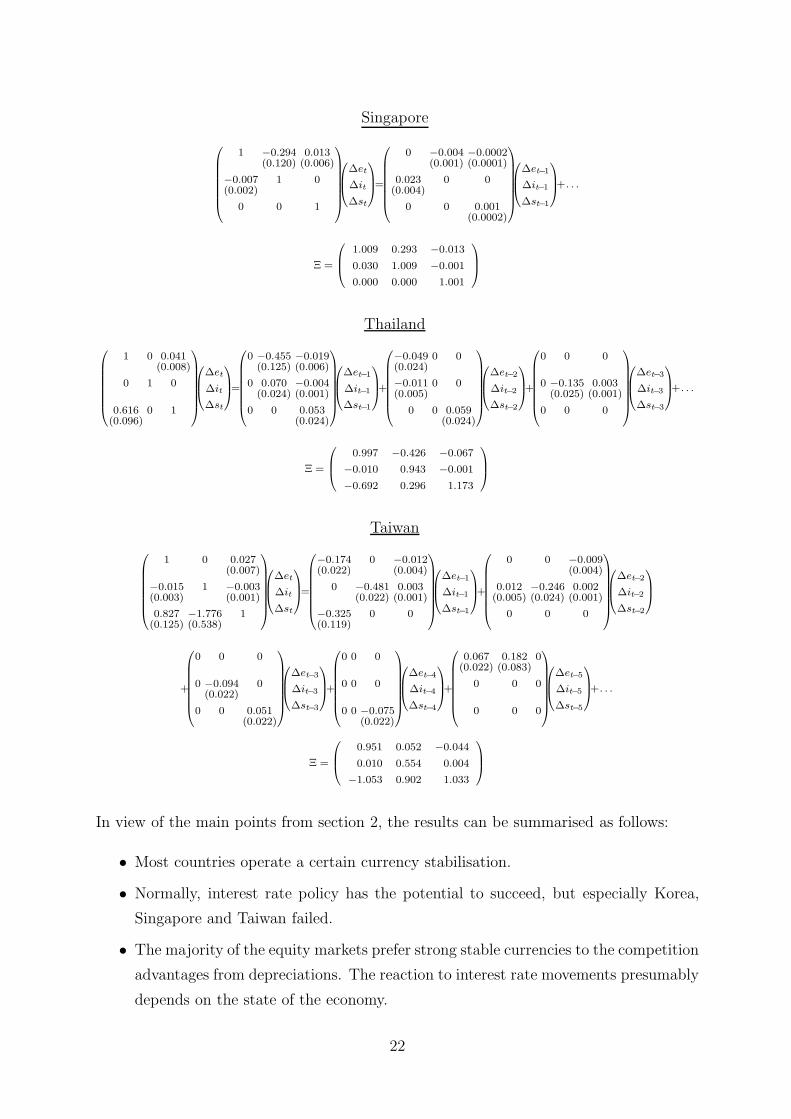
In view of the main points from section 2, the results can be summarised as follows:
• Most countries operate a certain currency stabilisation.
• Normally, interest rate policy has the potential to succeed, but especially Korea,
Singapore and Taiwan failed.
• The majority of the equity markets prefer strong stable currencies to the competition
advantages from depreciations. The reaction to interest rate movements presumably
depends on the state of the economy.
22
4.5 Common Regional Shocks
Until now, I have concentrated on level and volatility effects within models for the indi-
vidual countries. Naturally, the methodology can just as well be applied to estimating
systems including financial variables across different economies. In this paper however, I
take advantage of having identified the national economic disturbances to address regional
coherence: The following correlation analysis of the structural residuals should yield in-
formation not on the causal influences among the Asian Pacific countries, but on their
exposure to common shocks in the financial markets. Additionally, correlations among
the conditional variances could reveal common patterns in the sequence of volatile and
calm periods. This point of view gains its importance from the organisation of economic
cooperation in the Asian Pacific region, when for instance, symmetric innovations are
taken as prerequisites for an optimal South-East Asian currency area.
At first sight, Tables 6, 7 and 8 clarify, that relevant correlations exist only between the
exchange rate (mean = 0.24) and the stock market (mean = 0.29) shocks. In contrast,
the interest rate innovations (mean correlation = 0.03) seem to follow strong idiosyncratic
courses. Significance of the correlations is not assessed, because the high number of daily
observations allows almost no discrimination.
In the foreign exchange market, exceptions from the relatively strong linkages might be
Hong Kong, India, the Philippines and Taiwan; excluding these countries raises the mean
correlation to 0.35. For the former, the quasi dollar pegging comes as an obvious explana-
tion, India does of course not fit into the group of typical South-East Asian countries, and
the Philippines are characterised by an unstable economic environment with a number
of outliers. Interpreting the exchange rate correlations, one has to bear in mind, that
developments initiated by the US side are likely to have similar consequences on all con-
sidered currencies. While this describes a natural common factor for all exchange rates,
the variances are obviously less coherent (mean correlation = 0.12).
As has been mentioned above, the different money markets are not subject to relevant
common shocks. Contrary results might at most be found for the Oceanic countries
Australia and New Zealand as well as the cities of Hong Kong and Singapore. Evidently,
the markets are not governed by arbitrage mechanisms as described by the UIP, but
follow for example national monetary policy decisions. This result can be confirmed by
a cointegration analysis, producing hardly any evidence for commonness of stochastic
trends in the interest rates. The interpretation should nonetheless take into account, that
the turnovers in some of the national markets are quite low, rendering too far-reaching
23

AUS HK IDN INDIA JPN KOR NZL PLP SGP THL TWN
AUS × 0.05 0.04 0.18 0.21 -0.04 0.78 0.14 0.12 0.05 -0.05
HK 0.13 × -0.05 0.05 -0.03 -0.05 -0.04 -0.04 -0.01 0.07 0.02
IDN 0.22 0.10 × 0.17 0.09 0.10 0.10 0.25 0.27 0.13 0.08
INDIA 0.16 0.16 0.22 × 0.00 -0.01 0.28 -0.07 0.16 0.18 0.23
JPN 0.32 0.16 0.25 0.19 × 0.14 0.23 -0.05 0.33 0.14 0.11
KOR 0.16 0.11 0.30 0.16 0.32 × 0.03 0.08 0.34 0.34 0.24
NZL 0.77 0.11 0.18 0.14 0.27 0.15 × 0.10 0.15 0.23 0.09
PLP 0.08 0.03 0.28 0.07 0.14 0.20 0.09 × -0.04 0.07 0.03
SGP 0.37 0.17 0.35 0.24 0.58 0.36 0.36 0.22 × 0.36 0.15
THL 0.29 0.15 0.33 0.22 0.50 0.36 0.28 0.23 0.60 × 0.37
TWN 0.18 0.08 0.23 0.17 0.20 0.35 0.13 0.13 0.27 0.28 ×Table 6: Correlations of exchange rate shocks (lower left) and variances (upper right)
comparisons unreliable. The variances are correlated only slightly higher than the shocks
(mean=0.10), but for a cluster containing the industrialised economies of Hong Kong,
Japan, Korea, New Zealand and Singapore interest rate volatility is much more symmetric
(mean correlation=0.36). In contrast, the less developed markets seem to be disconnected
from any regional development.
AUS HK IDN INDIA JPN KOR NZL PLP SGP THL TWN
AUS × 0.03 0.02 0.12 -0.03 0.16 0.24 0.04 0.17 0.08 0.02
HK 0.10 × -0.05 0.21 0.34 0.28 0.47 -0.02 0.65 -0.00 -0.03
IDN -0.03 0.02 × -0.13 -0.06 0.06 0.07 -0.03 -0.10 0.05 -0.04
INDIA 0.02 0.05 0.00 × 0.26 0.16 0.18 0.05 0.41 0.06 -0.05
JPN 0.03 0.03 -0.01 0.02 × 0.08 0.26 -0.04 0.42 -0.02 -0.11
KOR 0.09 0.07 0.07 -0.01 -0.06 × 0.22 0.00 0.37 0.03 0.07
NZL 0.22 0.06 -0.04 -0.01 0.02 0.04 × -0.02 0.47 0.03 0.05
PLP 0.01 0.02 -0.03 -0.03 0.00 -0.00 0.03 × -0.04 0.02 0.01
SGP 0.07 0.22 -0.05 0.02 0.01 0.05 0.05 0.01 × 0.06 -0.00
THL 0.04 0.07 0.10 0.04 -0.01 0.03 0.04 0.06 0.07 × -0.01
TWN 0.03 0.02 -0.02 -0.03 0.01 0.04 0.06 0.01 0.01 0.03 ×Table 7: Correlations of interest rate shocks (lower left) and variances (upper right)
A totally different pattern can be established in the equity markets, where the most
coherent innovations are found. Deviations might at best be given in pairs including
24
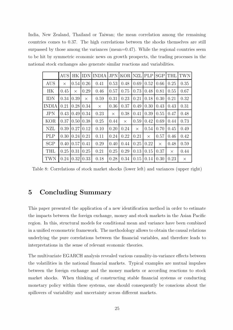
India, New Zealand, Thailand or Taiwan; the mean correlation among the remaining
countries comes to 0.37. The high correlations between the shocks themselves are still
surpassed by those among the variances (mean=0.47). While the regional countries seem
to be hit by symmetric economic news on growth prospects, the trading processes in the
national stock exchanges also generate similar reactions and variabilities.
AUS HK IDN INDIA JPN KOR NZL PLP SGP THL TWN
AUS × 0.54 0.26 0.41 0.53 0.48 0.69 0.52 0.66 0.25 0.35
HK 0.45 × 0.29 0.46 0.57 0.75 0.73 0.48 0.81 0.55 0.67
IDN 0.34 0.39 × 0.59 0.31 0.23 0.21 0.18 0.30 0.21 0.32
INDIA 0.21 0.28 0.34 × 0.36 0.37 0.49 0.30 0.43 0.43 0.31
JPN 0.43 0.49 0.34 0.23 × 0.38 0.41 0.39 0.55 0.47 0.48
KOR 0.37 0.50 0.38 0.25 0.44 × 0.59 0.42 0.69 0.44 0.73
NZL 0.39 0.27 0.12 0.10 0.20 0.24 × 0.54 0.70 0.45 0.49
PLP 0.30 0.24 0.21 0.11 0.24 0.22 0.21 × 0.57 0.46 0.42
SGP 0.40 0.57 0.41 0.29 0.40 0.44 0.25 0.22 × 0.48 0.59
THL 0.25 0.31 0.25 0.21 0.25 0.29 0.13 0.15 0.37 × 0.44
TWN 0.24 0.32 0.33 0.18 0.28 0.34 0.15 0.14 0.30 0.23 ×Table 8: Correlations of stock market shocks (lower left) and variances (upper right)
5 Concluding Summary
This paper presented the application of a new identification method in order to estimate
the impacts between the foreign exchange, money and stock markets in the Asian Pacific
region. In this, structural models for conditional mean and variance have been combined
in a unified econometric framework. The methodology allows to obtain the causal relations
underlying the pure correlations between the financial variables, and therefore leads to
interpretations in the sense of relevant economic theories.
The multivariate EGARCH analysis revealed various causality-in-variance effects between
the volatilities in the national financial markets. Typical examples are mutual impulses
between the foreign exchange and the money markets or according reactions to stock
market shocks. When thinking of constructing stable financial systems or conducting
monetary policy within these systems, one should consequently be conscious about the
spillovers of variability and uncertainty across different markets.
25

The identification of the important contemporaneous impacts allowed an interpretation
of financial interrelations in terms of causality: The short-term interest rates were found
to support the value of the domestic currencies, apart from few exceptions. For the bet-
ter part, the central banks should thus be able to stabilise the exchange rates of their
countries. Expectedly, the examination suggests, that most monetary authorities indeed
exploit this opportunity by reacting to currency fluctuations. Despite the official classifi-
cation as free floating, accordingly many exchange rate regimes seem still to be regulated
in some sense. One reason might be found in the stock markets, of which the majority
obviously prefers stable foreign exchanges to the export advantages of depreciating ten-
dencies. Opposingly, the evidence of money market rate influences on the stock market
is mixed: In one group of countries the straightforward negative effect prevails, but the
equity prices in another group rather seem to pick up the growth signals of rising interest
rates. At last, the appreciating propagation of positive equity shocks into the foreign
exchange market and the hardly relevant central bank reactions to such disturbances do
not come as a surprise.
Addressing the coherence of shocks in the Asian Pacific region, striking results could be
established: The highest correlations belong to the stock market residuals, suggesting
that growth innovations are fairly symmetric across the region. In contrast, international
money market linkages did not become evident. The foreign exchange markets revealed
clear signs of commonalities, at least for a cluster of economies.
Major actual political tasks in the Asian Pacific region include the stabilisation of the
financial system, the organisation of the future currency management and the backing of
sustained economic development. This research could give valuable information for all
these points. Future research might for example consider the task, if structural breaks
like the Asian financial crisis can be picked up by the variance process maintaining the
assumption of parameter constancy. A further type of interesting applications would be
given by including variables of different countries into one structural EGARCH model,
in order to address the international linkages directly. In this context, certain common
factors could be considered as an additional feature.
26

References
[1] Andersen, T.G., T. Bollerslev, F.X. Diebold, C. Vega (2005): Real-Time Price
Discovery in Stock, Bond and Foreign Exchange Markets. NBER Working Paper
W11312.
[2] Bautista, C.C. (2003): Interest Rate-Exchange Rate Dynamics in the Philippines: A
DCC Analysis. Applied Economics Letters, 10, 107-111.
[3] Berndt, E., B. Hall, R. Hall, J. Hausman (1974): Estimation and Inference in Non-
linear Structural Models. Annals of Social Measurement, 3, 653-665.
[4] Bollerslev, T., J.M. Wooldridge (1992): Quasi-Maximum Likelihood Estimation and
Inference in Dynamic Models with Time Varying Covariances. Econometric Reviews,
11, 143-172.
[5] Boyd, J.H., J. Hu, R. Jagannathan (2005): The Stock Market’s Reaction to Unem-
ployment News: Why Bad News Is Usually Good for Stocks. The Journal of Finance,
60, 649-672.
[6] Cappiello, L., R.A. De Santis (2005): Explaining exchange rate dynamics: The un-
covered equity return parity condition. ECB Working Paper 529.
[7] Caporale, G.M., A. Cipollini, P.O. Demetriades (2005): Monetary policy and the ex-
change rate during the Asian crisis: identification through heteroscedasticity. Journal
of International Money and Finance, 24, 39–53.
[8] Comte, F., O. Lieberman (2003): Asymptotic Theory for Multivariate GARCH Pro-
cesses. Journal of Multivariate Analysis, 84, 61–84.
[9] Dickey, D.A., W.A. Fuller (1979): Distribution of the Estimators for Autoregressive
Time Series with a Unit Root. Journal of the American Statistical Association, 74,
427-431.
[10] Doornik, J.A. (1996): Testing vector error autocorrelation and heteroscedasticity.
Unpublished paper, Nullfield College.
[11] Doornik, J.A. (1998): Approximations to the asymptotic distributions of cointegra-
tion tests. Journal of Economic Surveys, 12, 573-593.
[12] Johansen, S. (1994): The role of the constant and linear terms in cointegration
analysis of nonstationary time series. Econometric Reviews, 13, 205-231.
27

[13] Johansen, S. (1995): Likelihood-based Inference in Cointegrated Vector Autoregres-
sive Models. Oxford University Press, Oxford.
[14] MacKinnon, J.G. (1991): Critical Values for Cointegration Tests. Chapter 13 in
R.F. Engle, Granger, C.W.J. (eds.): Long-run Economic Relationships: Readings in
Cointegration, Oxford University Press, Oxford.
[15] MacKinnon, J.G. (1996): Numerical Distribution Functions for Unit Root and Coin-
tegration Tests. Journal of Applied Econometrics, 11, 601-618.
[16] Lee, K.Y. (2006): The contemporaneous interactions between the U.S., Japan, and
Hong Kong stock markets. Economics Letters, 90, 21–27.
[17] Nelson, D.B. (1991): Conditional Heteroskedasticity in Asset Returns: A New Ap-
proach. Econometrica, 59, 347-370.
[18] Rigobon, R. (2003): Identification through heteroscedasticity. Review of Economics
and Statistics, 85, 777-792.
[19] Rigobon, R., B. Sack (2003a): Measuring the reaction of monetary policy to the
stock market. Quarterly Journal of Economics, 118, 639–669.
[20] Rigobon, R., B. Sack (2003b): Spillovers across U.S. financial markets. Working
Paper, Sloan School of Management, MIT and NBER.
[21] Stiglitz, J.E. (1999): Interest rates, risk, and imperfect markets: puzzles and policies.
Oxford Review of Economic Policy, 15, 59–76.
28
Appendix
0.1
0.2
0.3
0.4
0.5
0.6
0.7
0.8
0.9
1.0
1999 2000 2001 2002 2003 2004 2005 2006
AUS_VAR_E
.000
.001
.002
.003
.004
.005
.006
.007
.008
1999 2000 2001 2002 2003 2004 2005 2006
AUS_VAR_I
0.0
0.4
0.8
1.2
1.6
2.0
2.4
1999 2000 2001 2002 2003 2004 2005 2006
AUS_VAR_S
.00
.01
.02
.03
.04
1999 2000 2001 2002 2003 2004 2005 2006
HK_VAR_E
.00
.02
.04
.06
.08
.10
1999 2000 2001 2002 2003 2004 2005 2006
HK_VAR_I
0
1
2
3
4
5
6
7
1999 2000 2001 2002 2003 2004 2005 2006
HK_VAR_S
0.0
0.4
0.8
1.2
1.6
1999 2000 2001 2002 2003 2004 2005 2006
I DN_VAR_E
.00
.04
.08
.12
.16
.20
.24
.28
1999 2000 2001 2002 2003 2004 2005 2006
I DN_VAR_I
0
1
2
3
4
5
6
1999 2000 2001 2002 2003 2004 2005 2006
I DN_VAR_S
.0
.1
.2
.3
.4
.5
.6
1999 2000 2001 2002 2003 2004 2005 2006
I NDI A_VAR_E
.00
.01
.02
.03
.04
.05
.06
.07
.08
1999 2000 2001 2002 2003 2004 2005 2006
I NDI A_VAR_I
0
4
8
12
16
20
1999 2000 2001 2002 2003 2004 2005 2006
I NDI A_VAR_S
.1
.2
.3
.4
.5
.6
.7
1999 2000 2001 2002 2003 2004 2005 2006
JPN_VAR_E
.0000
.0004
.0008
.0012
.0016
1999 2000 2001 2002 2003 2004 2005 2006
JPN_VAR_I
0
1
2
3
4
5
6
7
8
1999 2000 2001 2002 2003 2004 2005 2006
JPN_VAR_S
29

.0
.1
.2
.3
.4
.5
.6
.7
.8
1999 2000 2001 2002 2003 2004 2005 2006
KOR_VAR_E
.000
.005
.010
.015
.020
.025
.030
1999 2000 2001 2002 2003 2004 2005 2006
KOR_VAR_I
0
2
4
6
8
10
12
14
1999 2000 2001 2002 2003 2004 2005 2006
KOR_VAR_S
0.3
0.4
0.5
0.6
0.7
0.8
0.9
1.0
1.1
1999 2000 2001 2002 2003 2004 2005 2006
NZL_VAR_E
.000
.002
.004
.006
.008
.010
1999 2000 2001 2002 2003 2004 2005 2006
NZL_VAR_I
0.0
0.4
0.8
1.2
1.6
2.0
2.4
2.8
1999 2000 2001 2002 2003 2004 2005 2006
NZL_VAR_S
0.0
0.4
0.8
1.2
1.6
2.0
1999 2000 2001 2002 2003 2004 2005 2006
PLP_VAR_E
0
1
2
3
4
1999 2000 2001 2002 2003 2004 2005 2006
PLP_VAR_I
0
1
2
3
4
5
6
1999 2000 2001 2002 2003 2004 2005 2006
PLP_VAR_S
.00
.04
.08
.12
.16
.20
1999 2000 2001 2002 2003 2004 2005 2006
SGP_VAR_E
.000
.004
.008
.012
.016
.020
1999 2000 2001 2002 2003 2004 2005 2006
SGP_VAR_I
0
1
2
3
4
5
6
1999 2000 2001 2002 2003 2004 2005 2006
SGP_VAR_S
.0
.1
.2
.3
.4
.5
.6
.7
1999 2000 2001 2002 2003 2004 2005 2006
THL_VAR_E
.00
.01
.02
.03
.04
.05
.06
.07
1999 2000 2001 2002 2003 2004 2005 2006
THL_VAR_I
0
1
2
3
4
5
6
7
1999 2000 2001 2002 2003 2004 2005 2006
THL_VAR_S
.0
.1
.2
.3
.4
.5
.6
1999 2000 2001 2002 2003 2004 2005 2006
TW N_VAR_E
.00
.01
.02
.03
.04
.05
.06
1999 2000 2001 2002 2003 2004 2005 2006
TW N_VAR_I
0
2
4
6
8
10
12
14
1999 2000 2001 2002 2003 2004 2005 2006
TW N_VAR_S
Figure 2: Conditional variances of foreign exchange, money and stock market innovations
30

SFB 649 Discussion Paper Series 2007
For a complete list of Discussion Papers published by the SFB 649, please visit http://sfb649.wiwi.hu-berlin.de.
001 "Trade Liberalisation, Process and Product Innovation, and Relative Skill Demand" by Sebastian Braun, January 2007. 002 "Robust Risk Management. Accounting for Nonstationarity and Heavy Tails" by Ying Chen and Vladimir Spokoiny, January 2007. 003 "Explaining Asset Prices with External Habits and Wage Rigidities in a DSGE Model." by Harald Uhlig, January 2007. 004 "Volatility and Causality in Asia Pacific Financial Markets" by Enzo Weber, January 2007.
SFB 649, Spandauer Straße 1, D-10178 Berlin http://sfb649.wiwi.hu-berlin.de
This research was supported by the Deutsche
Forschungsgemeinschaft through the SFB 649 "Economic Risk".


