
Image Processing Applicationsa.k.a
Computational Photography
Dr. Shai AvidanFaculty of Engineering
Tel-Aviv University

Slide Credits (partial list)
• Rick Szeliski• Steve Seitz• Alyosha Efros• Yacov Hel-Or• Yossi Rubner• Miki Elad• Marc Levoy• Bill Freeman• Fredo Durand• Sylvain Paris

Grade Policy• Exam 40%• 3 Matlab projects each 20%

What I did not talk about• Camera Arrays• Light Fields• Coded Aperture• Sparse Codes• …

Syllabus• Sampling/Resampling• Image Pyramids• Image Warping• Image Retargeting
– Seam Carving– Inhomogeneous image scaling– Bidirectional Similarity– ShiftMap
• Gradient Domain Image Editing– Poisson Equation
• Edge Preserving Filters– Bilateral Filter– Anisotropic Diffusion– Non-local Means– Robust Statistics
• Wavelets• Image Completion• Texture Synthesis• Super Resolution• Optical Flow

Sampling/Resampling• Image Acquisition pipeline• Reconstruction conditions (Nyquist rate)• The Ideal Low-pass filter• Aliasing• Image scaling (up-sampling/down-sampling)• Resampling• Image warp (Forward/Backward mapping)

Image Pyramids• Gaussian Pyramid• Laplacian Pyramid
Applications:• Image blending• Texture Synthesis

Image Retargeting• What is image retargeting?• Seam Carving• Inhomogeneous image scaling• Bidirectional Similarity• Shift Map

Gradient Domain• Gradient Field• Laplace/Poisson Equation• Conjugate Gradient
Applications• Image inpainting• Image stitching• High Dynamic Range compression• RGB2Gray

Edge Preserving Filtering• Bilateral Filtering
– Cross Bilateral Filtering• Weighted Least Squares• Robust Statistics
– Line Process• Anisotropic Diffusion
– Scale Space• Connections between the different methods• Non-Local Means
Applications:• Edge Preserving Smoothing• Image Denoising• HDR Compression

Wavelets• The wavelet and inverse wavelet transforms
– Basis function– Scaling function
• Wavelet Lifting
Applications:• Wavelet Compression• Wavelet Shrinkage for image denoising

Texture Synthesis• Heeger-Bergen• DeBonet• Exemplar based methods
– Efros and Leung– Image Quilting– Criminisi et al.– Global Objective Function– K-coherence– PatchMatch– Internet-based

Super Resolution• HR from multiple LR images
– ML approach– MAP approach
• Exemplar-based Super Resolution– Nearest Neighbors– MRF model– Single scan
• Single Image SR

Optical Flow• Constant Brightness Assumption• Constant Brightness Equation• Normal Flow• Aperture Problem• Lucas-Kanade• Horn-Schunk

Three Methods for Resizing Images

Resampling
8×××× 16××××nearest neighbornearest neighbor nearest neighbornearest neighbor
bicubic interpolationbicubic interpolation bicubic interpolationbicubic interpolation
(resizing)


Super Resolution
• What if we have more than one image?– Either we have multiple low resolution
images– Or we have a database of low/high image
patches to rely on

Cubic Spline
Original70x70
Examplebased, training:generic
True280x280
Super Resolution

Scaling
Input Output

Retargeting
Non-Homogeneous[Wolf et al., ICCV’07]
Optimized Scale and Stretch [Wang at el, SIGGRAPH Asia’08]
Improved Seam Carving [Robinstein et al, SIGGRAPH’08]
Shift-Maps

Scaling
Input Output

Retargeting
Non-Homogeneous[Wolf et al., ICCV’07]
Optimized Scale and Stretch [Wang at el, SIGGRAPH Asia’08]
Improved Seam Carving [Robinstein et al, SIGGRAPH’08]
Shift-Maps

morphing
cross-fading
Image morphingimage #1 image #2
warp warp

Multiband Blending: example

© prof. dmartin
Multiband Blending: example

Editing in Gradient Domain
• Given vector field G=(u(x,y),v(x,y)) (pasted gradient) in a bounded region Ω. Find the values of f in Ω that optimize:
Ω∂∗
Ω∂Ω=−∇∫∫ ffwithGf
f
2min
G=(u,v)
f*
fI
f*
Ω

Image Compositing

2D case
From Perez et al. 2003

2D case
From Perez et al. 2003

2D case

Transparent CloningTransparent Cloning
I SΩ Ω∇ =∇2
S TI Ω ΩΩ
∇ +∇∇ = ( )max ,I S TΩ Ω Ω∇ = ∇ ∇
Possible Quiz Question

High Dynamic Range Images
Local tone mappingSimple contrast reduction


Bilateral Filter
• How to extend the Gaussian Filter?• What’s the problem with Gaussian
Filter?

space
Gaussian Blur and Bilateral Filter
space rangenormalization
Gaussian blur
( ) ( )∑∈
−−=S
IIIGGW
IBFq
qqpp
p qp ||||||1
][rs σσ
Bilateral filter[Aurich 95, Smith 97, Tomasi 98]
space
space
range
p
p
q
q
( )∑∈
−=S
IGIGBq
qp qp ||||][ σ

pp
Bilateral Filter on a Height Field
output input
( ) ( )∑∈
−−=S
IIIGGW
IBFq
qqpp
p qp ||||||1
][rs σσ
pp
reproducedfrom [Durand 02]

σs= 2
σs= 6
σs= 18
σr = 0.1 σr = 0.25σr = ∞
(Gaussian blur)
input
Exploring the Parameter SpaceExploring the Parameter Space
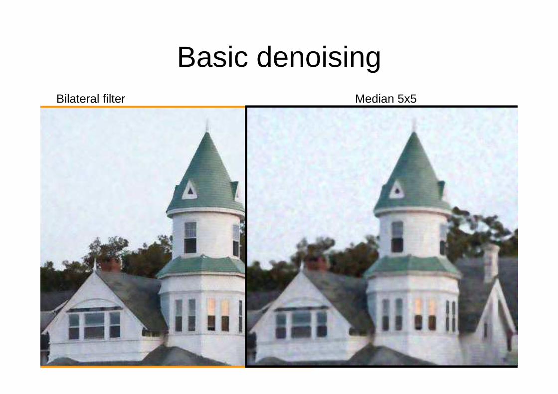
Bilateral filter
Basic denoisingMedian 5x5

Flash / No-Flash Photo Improvement(Petschnigg04) (Eisemann04)
Merge best features: warm, cozy candle light (no-flash)low-noise, detailed flash image

Petschnigg:
• Flash

Petschnigg:
• No Flash,

Petschnigg:
• Result

Another way to look at Denoising• What we want is to recover a signal X that is smooth. So lets define the
following objective function:Weighted Least Squares:
Robust Estimation
The matrix D stands for a one-sample shift to the right. Thus, the term (X-DX) is simply a discrete approximation of a backward first derivative. If Z = X-DX, then Z[k] = X[k]-X[k-1]. For example

BF is a single iteration of Jacobi method• BF is merely a single iteration of the Jacobi algorithm ,using the
objective function:
• This function is different from the one used by WLS/RE in the regularization term. Whereas WLS/RE penalizes smoothness with the first neighboring pixels, the new term penalizes nonsmoothness with distant pixels as well.

Anisotropic Diffusion
divergence gradient Laplacian
This reduces toe the isotropic heat diffusion equation if c(x,y,t)=const.
Suppose we knew at time (scale) t, the location of region bounariesappropriate for that scale. We would want to encourage smoothingwithin a region in preference to smoothing across boundaries.This could be achieved by setting the conduction coefficient to be 1 in the interior of each region and 0 at the boundary.
The problem: We don’t know the boundaries!
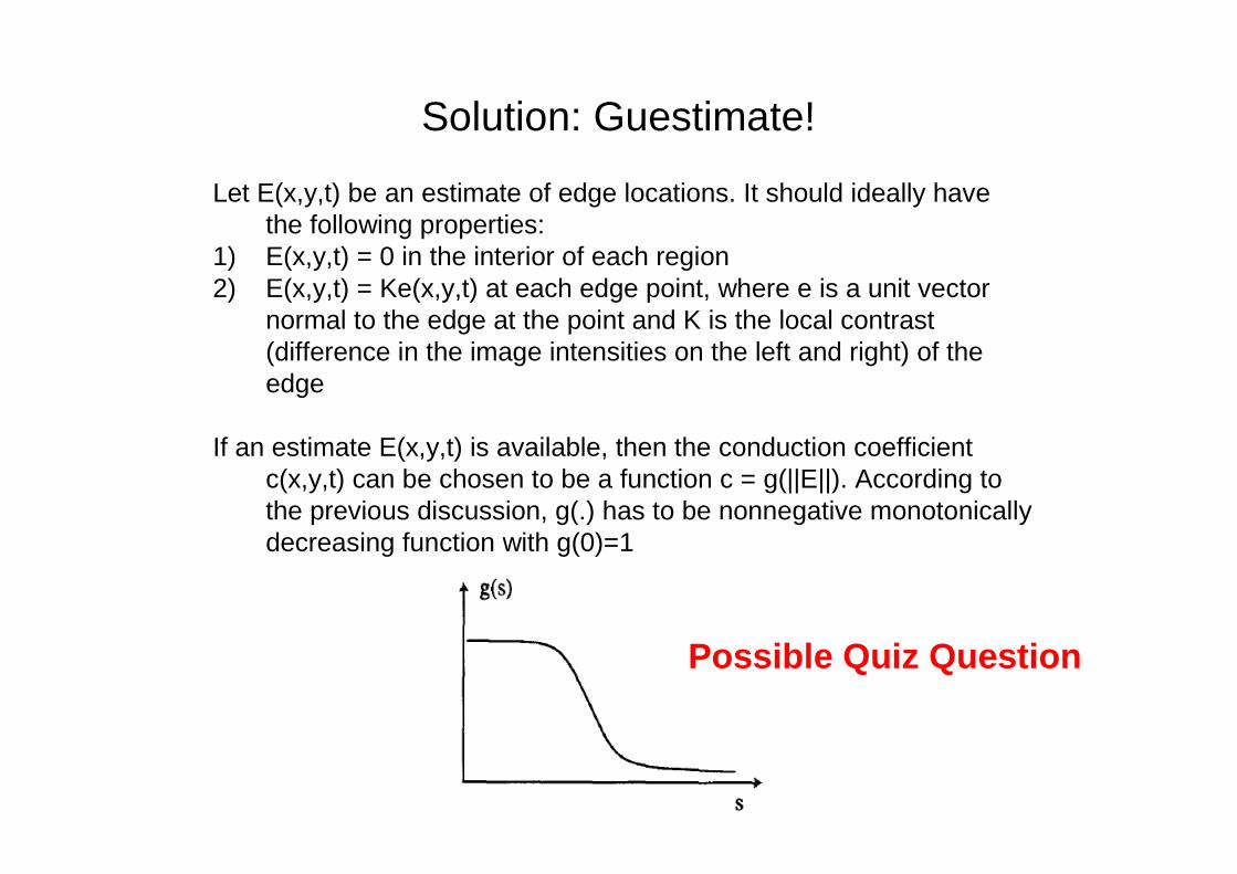
Solution: Guestimate!
Let E(x,y,t) be an estimate of edge locations. It should ideally have the following properties:
1) E(x,y,t) = 0 in the interior of each region2) E(x,y,t) = Ke(x,y,t) at each edge point, where e is a unit vector
normal to the edge at the point and K is the local contrast (difference in the image intensities on the left and right) of the edge
If an estimate E(x,y,t) is available, then the conduction coefficient c(x,y,t) can be chosen to be a function c = g(||E||). According to the previous discussion, g(.) has to be nonnegative monotonically decreasing function with g(0)=1
Possible Quiz Question

The choice of function phi()=g(Ix)Ix that leads to edge enhancement
When phi increases, its derivative is greater than zero and the edge will get blurred. At some point, \phi decreases and the edge will be enhanced. The g functions used in the paper are:
Possible Quiz Question

The basic 2x2 wavelet transform
Lets start with a simple transform
Given signal [a,b] we obtain [c,d]Given [c,d] we can recover [a,b]Observe that c is sum of elements and d is their difference
The scaling function: [1 1]The wavelet function: [-1 1]

Wavelet Shrinkage Pipeline

Wavelet Shrinkage Denoising

Texture Synthesis
• Histogram matching• Data Driven• Image/Video

Texture Synthesiswhite bread brick wall

“Onion skin” filling order

Structure guided filling
Original image Image with holeFilling in “onion skin”
orderStructure guided filling
Possible Quiz Question

Image Completion by Example-Based Inpainting
• A. Criminisi, P. Perez, and K. Toyama, CVPR 2003


Video
• Super resolution• Optic-flow
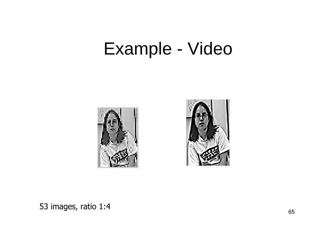
Example - Video
53 images, ratio 1:465
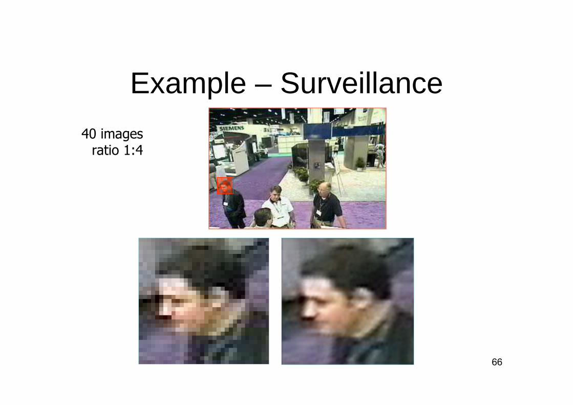
40 images ratio 1:4
Example – Surveillance
66

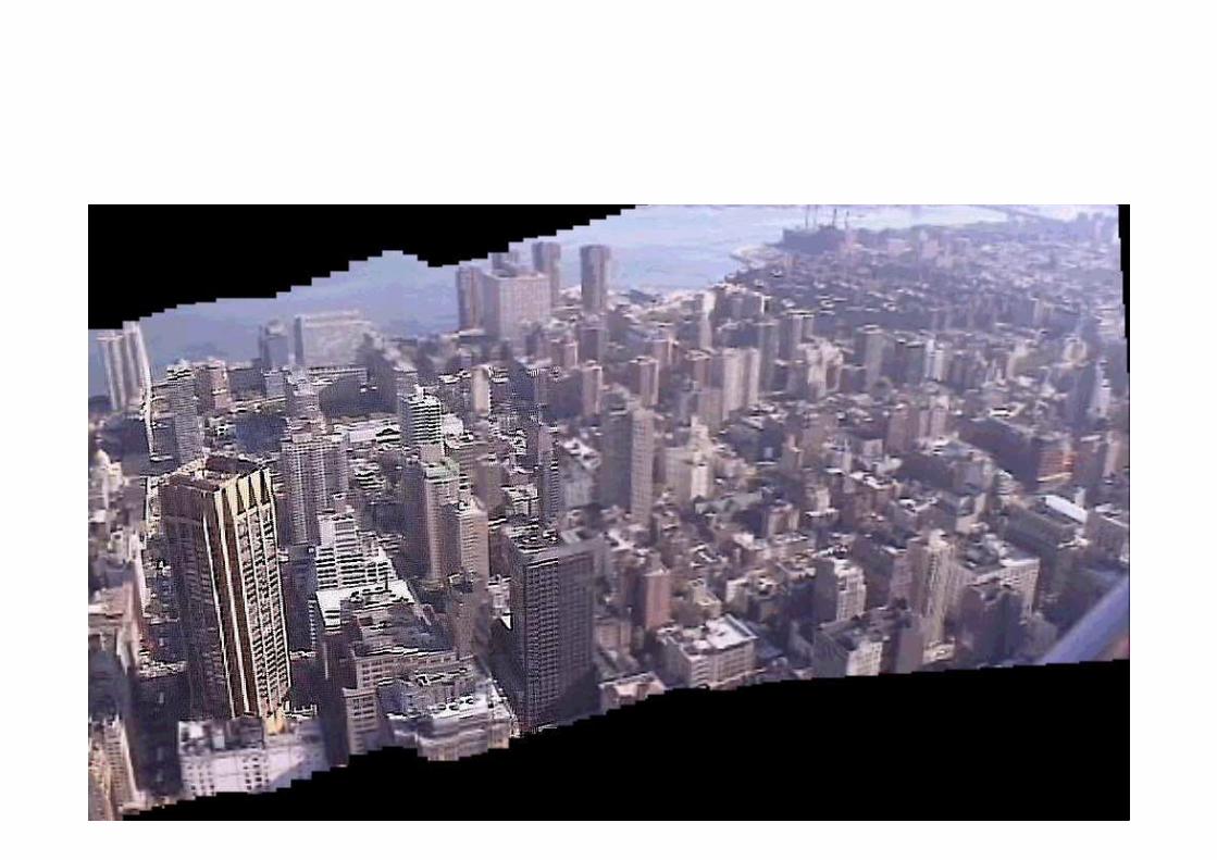
Example – Enhance Mosaics
67
68

Optical Flow
Pierre Kornprobst's Demo

Examples of Motion fields
Forward motion
Rotation Horizontal translation
Closer objects
appear to move faster!!

Example Quiz Questions 11. Image Retargeting
a. What is Image Retargeting? Describe one discrete and one continues method for solving the problem.b. Inhomogenous image scaling generates a forward map on a quad-mesh. How would you convert forward mapping to backward mapping? And why should you do that? c. Explain how to use Shift-Map for image reshuffling
2. Bilateral Filtera. Give the Bilateral Filter equation and explain how does it differ from a Weighted Least Squares approach?b. Explain Cross Bilateral Filter and how it is usedc. Give an example image where Bilateral Filter and Anisotropic Diffusion behave differently.
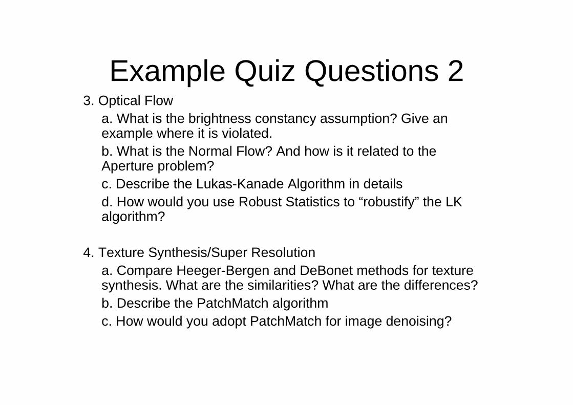
Example Quiz Questions 23. Optical Flow
a. What is the brightness constancy assumption? Give an example where it is violated.b. What is the Normal Flow? And how is it related to the Aperture problem?c. Describe the Lukas-Kanade Algorithm in detailsd. How would you use Robust Statistics to “robustify” the LK algorithm?
4. Texture Synthesis/Super Resolutiona. Compare Heeger-Bergen and DeBonet methods for texture synthesis. What are the similarities? What are the differences?b. Describe the PatchMatch algorithmc. How would you adopt PatchMatch for image denoising?


