
Working Paper Researchby Ayumu Ken Kikkawa, Glenn Magerman, Emmanuel Dhyne
January 2019 No 363
Imperfect competition in firm-to-firm trade
NBB WORKING PAPER No. 363 – JANUARY 2019
Editor
Pierre Wunsch, Governor of the National Bank of Belgium
Statement of purpose:
The purpose of these working papers is to promote the circulation of research results (Research Series) and analytical studies(Documents Series) made within the National Bank of Belgium or presented by external economists in seminars, conferencesand conventions organised by the Bank. The aim is therefore to provide a platform for discussion. The opinions expressed arestrictly those of the authors and do not necessarily reflect the views of the National Bank of Belgium.
Orders
For orders and information on subscriptions and reductions: National Bank of Belgium,Documentation - Publications service, boulevard de Berlaimont 14, 1000 Brussels
Tel +32 2 221 20 33 - Fax +32 2 21 30 42
The Working Papers are available on the website of the Bank: http://www.nbb.be
© National Bank of Belgium, Brussels
All rights reserved.Reproduction for educational and non-commercial purposes is permitted provided that the source is acknowledged.
ISSN: 1375-680X (print)ISSN: 1784-2476 (online)
NBB WORKING PAPER No. 363 – JANUARY 2019
Abstract
This paper studies the implications of imperfect competition in firm-to-firm trade. Using a dataset on
all transactions between Belgian firms, we find that firms charge higher markups if they have higher
input shares among their buyers. We interpret this as firms competing as oligopolies to supply inputs
to each buyer and build a model in which they charge different markups to different buyers. We use
the estimated model to quantify how distortionary firm-to-firm markups are. Reducing all markups infirm-to-firm trade by 20 percent increases welfare by around 7 percent, suggesting large distortions
due to double marginalization. We then investigate how endogenous markups in firm-to-firm trade
alter predictions of the transmission of shocks. In the counterfactual where we take a fall in import
prices as the shock, we show that allowing for oligopolistic competition generates larger cost
reductions for some firms, and attenuates these for others relative to a case with constant markups.
We demonstrate that a measure capturing firms’ positions in the production chain is a key metric in
explaining this heterogeneity.
JEL codes: F12, L13, L14
Keywords: Firm-to-firm networks, imperfect competition
Authors:Ayumu Ken Kikkawa, Sauder School of Business, University of British Columbia
- e-mail: [email protected] Magerman, Université Libre de Bruxelles - e-mail: [email protected] Dhyne, National Bank of Belgium and University of Mons
- e-mail: [email protected]
First version: November 2017. This paper was previously circulated under the title ”ImperfectCompetition and the Transmission of Shocks: The Network Matters.” Part of the analyses was donewhen Kikkawa was at the National Bank of Belgium as a researcher. The views expressed in thispaper are those of the authors and do not necessarily reflect the views of the National Bank of Belgiumor any other institution with which the authors are affiliated. We would like to thank Felix Tintelnot,Brent Neiman, Chad Syverson, Magne Mogstad, Costas Arkolakis, Jonathan Dingel, Jonathan Eaton,Rodrigo Adao, Yves Zenou, Yuta Takahashi, Yuan Mei, Pablo Robles, and Mons Chan for theirvaluable advisement, and Michal Fabinger, Teresa Fort, and Kevin Lim for helpful discussions.Kikkawa gratefully acknowledges the financial support of the University of Chicago Department ofEconomics Travel Grant. We would also like to thank the National Bank of Belgium for access to itsdatasets and for its assistance.
The views expressed in this paper are those of the authors and do not necessarily reflect the viewsof the National Bank of Belgium or any other institutions to which the authors are affiliated.

NBB WORKING PAPER No. 363 – JANUARY 2019

NBB WORKING PAPER – No. 363 – JANUARY 2019
TABLE OF CONTENTS
1. Introduction ........................................................................................................................ 1
2. Data and evidence .............................................................................................................. 62.1 Dataset and sample selection............................................................................................... 6
2.2 Skewed input shares across suppliers .................................................................................. 7
2.3 Markups and input shares .................................................................................................... 8
3. Model ................................................................................................................................ 12
3.1 Preference ......................................................................................................................... 12
3.2 Technology and market structure ....................................................................................... 13
3.3 Equilibrium ......................................................................................................................... 16
3.4 Alternative models as benchmarks ..................................................................................... 17
4. Estimation ........................................................................................................................ 19
5. How distortionary are markups in firm-to-firm trade? .................................................... 23
6. How do markups in firm-to-firm trade alter predictions of the transmissionof shocks? ........................................................................................................................ 28
7. Conclusion ....................................................................................................................... 35
References .................................................................................................................................. 36
Tables.......................................................................................................................................... 43
National Bank of Belgium - Working papers series ....................................................................... 85

NBB WORKING PAPER No. 363 – JANUARY 2019

1 Introduction
Firms largely operate and compete in relationships with other firms. Firms often deliver their output to
multiple firms, and they often purchase inputs from multiple firms. These buyer-supplier relationships
create a complex network of firm-to-firm transactions. One such complexity is that the set of firms
that a firm competes against when supplying to a certain buyer may be different from those when
supplying to a different buyer. This paper studies the nature of this competition in firm-to-firm trade
and analyzes its implications.
We examine detailed administrative data on all domestic firm-to-firm transactions in Belgium.
We explore and quantify to what extent firms engage in imperfect competition when they sell their
outputs to each individual firm. In Belgium, the firm-to-firm network is extremely sparse, and firms’
outputs pass through many other firms until they reach final demand. To the extent that firms are in
non-competitive environments when they engage in firm-to-firm trade, the distortions they face due to
firm-to-firm markups are likely heterogeneous depending on how downstream they are. Quantifica-
tion of these distortions requires accounting for the underlying structure of the firm-to-firm network.
We also explore the implications that markups in firm-to-firm trade have on counterfactual pre-
dictions. The Belgian data reveals large skewness in the input shares firms have across suppliers. If
these input shares reflect suppliers’ abilities to charge markups, then accounting for the endogene-
ity of markups for each firm-to-firm pair becomes important when analyzing how shocks transmit
through the economy. In response to shocks, firm-to-firm markups may change through changing
firm-to-firm input shares, thus attenuating or amplifying both firm-level and aggregate outcomes.
The data points out to the importance of focusing on firm-to-firm relationships when studying
firms’ competition. We find that firms charge higher average markups when they have larger input
shares amongst their buyers. Firm-level average markups are measured by either computing ac-
counting markups or estimating markups following De Loecker and Warzynski (2012). This positive
relationship holds even after controlling for the firms’ sectoral market shares. We interpret this fact
as firms competing as oligopolies to supply inputs to each buyer. In addition to the firm-level market
share within a sector, the firm’s pairwise input shares for each buyer capture the pair-level pricing
power the firm has for each of its buyers.
Motivated by this fact, we build a model of oligopolistic competition in firm-to-firm trade. With
a nested CES structure in the production function that builds on Atkeson and Burstein (2008), firms
charge different markups to each buyer firm. The more conventional implementation is where a firm’s
total sales share among same-sector firms determines its firm-level markup; in our model, the markup
a firm charges a buyer depends on the firm’s share in the buyer’s intermediate goods purchases. As
firms compete with different sets of firms when selling to each buyer, the shares that firms have in
each buyer’s intermediate goods vary across buyers. Therefore, the model puts emphasis on the firms’
1

pricing powers that vary across buyers.
Mapping the data to our model, we estimate the CES parameters in both preference and produc-
tion functions. We obtain these estimates so that the firm-level average markups – averages of the
model implied markups on sales to other producers and to the final consumer – provide the best fit of
those implied by the data. The estimated CES parameters reveal that firms generally charge higher
markups in their sales to other firms than in their sales to final demand.
Equipped with these estimates, we conduct two separate counterfactual exercises that explore
the implications of oligopolistic competition in firm-to-firm trade. In the first counterfactual exer-
cise, we quantify how distortionary firm-to-firm markups are. With each firm along the production
chain charging a different markup in the observed firm-to-firm trade network, the degree of double
marginalization can be large. From the estimated model we back out markups for each buyer-supplier
pair in the data and consider the reduction in those markups in firm-to-firm trade as the shock. We
find that in response to a 20 percent reduction in firm-to-firm markups, aggregate welfare – measured
as the level of household consumption – increases by 7 percent.
We contrast these results to those obtained by assuming a sectoral roundabout production econ-
omy. In the sectoral roundabout production economy we impose a simple network structure in which
there are two sets of common composite goods, one of which is used as intermediate goods and
the other as final consumption goods. In this exercise we keep the initial firm-level sales, firm-level
inputs, firms’ markups charged on sales to final demand, and firm-level average markups on interme-
diate goods sales consistent with our model. The impact of the markup reduction on welfare turns
out to be smaller under the sectoral roundabout production economy: in response to a 20 percent re-
duction in markups charged on common composite intermediate goods, aggregate welfare increases
by less than 5 percent. Failing to fully account for the observed firm-to-firm trade network leads to a
smaller magnitude of distortion because the sectoral roundabout production economy cannot capture
the heterogeneity in cost reductions that firms face. Under the observed firm-to-firm trade network,
some firms that are downstream experience extreme cost reductions leading to greater movements in
the aggregate due to non-linearities in the system.
In the second counterfactual exercise we explore how oligopolistic competition in firm-to-firm
trade affects predictions of the transmission of shocks both at the firm-level and at the aggregate level.
We shock an exogenous parameter in the model – the price of foreign goods – and see how the model’s
predictions differ from those without endogenous markups in firm-to-firm trade. As a benchmark, we
consider a special case of the model where we impose markups that are heterogeneous across buyers
but constant.
Implementing endogenous markups leads to two counteracting effects on top of the effects pre-
dicted under constant markups. First, endogenous markups imply an incomplete pass-through from
a change in the supplier’s input price to the change in its output price. When the price of foreign
2

goods fall, firms may increase their markups in response to reductions in their input costs. We call
this the “attenuation effect,” as firms’ cost changes are not fully passed on to their buyers attenuating
both firm-level and aggregate responses. Second, when a firm faces a reduction in its input costs, the
other suppliers that sell goods to the firm’s buyers may reduce their markups in the face of increased
competition. We call this the “pro-competitive effect,” as this amplifies the downstream effects of
cost reductions.
We characterize the magnitudes of these two counteracting effects operating within each buyer-
supplier pair. We find it important to account for endogenous markups in firm-to-firm trade to under-
stand cost changes at the firm-level. In response to a foreign price change, around half of the firms
face higher markups from their suppliers on average while the rest face lower markups. We demon-
strate that a measure capturing the firms’ respective positions in the production chain is a key metric
in explaining this heterogeneity. The more exposed a firm is to foreign inputs through its domestic
suppliers, the higher markups the firm faces from its suppliers on average. And overall, under the
uniform foreign price reduction that reduces the costs of all importers directly and of almost all firms
indirectly, we find that accounting for endogenous markups in firm-to-firm trade has quantitatively
small effects on aggregate welfare. The two counteracting effects largely cancel each other out in the
aggregate.
This paper contributes to the literature studying the implications of imperfect competition in inter-
mediate goods markets. Grassi (2018) develops a model in which firms engage in oligopolistic com-
petition in an economy with sectoral input-output linkages and studies the contribution of firm-level
shocks on the aggregate dynamics.1 Effects similar to our attenuation and pro-competitive effects
are studied extensively in other contexts. For example, Feenstra, Gagnon, and Knetter (1996) study
how the degree of price pass-through varies with the firm’s export market share. Amiti, Itskhoki,
and Konings (2017) study how firms’ prices respond to changes in the prices of their competitors.
Atkeson and Burstein (2008) focus on incomplete price pass-through to explain deviations of interna-
tional relative prices from relative PPP. These papers analyze oligopolistic competition where firms
compete with others within the same sector, implying that the firm’s market power is captured by its
market share in its sector.2 In contrast, we propose a more granular view on the competition between
firms. In addition to the firm-level market share within the sector being the determinant of the firm’s
market power, we suggest that the pair-level input shares across its buyers are also relevant metrics
1As in Grassi (2018), we focus on strategic complementarities across suppliers in the style of Atkeson and Burstein(2008). See Neiman (2011) for a similar model of variable markups that allows for arm’s length and intra-firm trans-actions. Mongey (2018) studies inflation and output responses to monetary shocks in oligopolistic market structures.Morlacco (2018) and Macedoni and Tyazhelnikov (2018) cast attention to firms’ market power as buyers of goods ininternational markets. For imperfect competition where complementarities arise from the demand side, see also Krugman(1979), Ottaviano, Tabuchi, and Thisse (2002), Melitz and Ottaviano (2008), and Zhelobodko, Kokovin, Parenti, andThisse (2012).
2There are also cases in which aggregate volatilities can be captured by the distribution of market shares. See for ex-ample Gabaix (2011), where the Herfindahl-Hirschman Index (HHI) is the main metric that captures aggregate volatility.
3
in capturing the firm’s ability to charge markups.
This paper is also related to the vast literature investigating the implications of distortions. Our
approach to assess the quantitative impact of distortions is similar to those in Restuccia and Rogerson
(2008) and Hsieh and Klenow (2009), in which they compute the aggregate counterfactuals upon
hypothetical reductions of wedges.3 We focus on a particular source of distortions, imperfect compe-
tition in firm-to-firm trade, and quantify how much distortion it creates in the aggregate. Focusing on
imperfect competition in firm-to-firm trade also connects our paper to research on on firm boundaries
and vertical relationships, seminally developed by Coase (1937). Our findings that reducing markups
in firm-to-firm transactions can substantially lower firms’ costs relate our paper to the literature study-
ing incentives of firms to vertically integrate. The efficiency motive for vertical integration has been
intensively studied and empirically investigated for selected sectors (see Lafontaine and Slade, 2007,
for a survey on this literature).4
We also relate this paper to the important work by Baqaee and Farhi (2018), which provides a
framework for aggregating micro shocks at the first-order or second-order approximation, using a
general model with distortions such as markups.5 Using U.S. firm-level data, they find that eliminat-
ing firm-level markups would increase aggregate TFP by around 20 percent.6 In this paper we capture
the heterogeneous markups firms potentially charge different buyers and investigate the distortions
created by markups in firm-to-firm trade. The markups we back out using the structure of the model
are generally higher in firm-to-firm trade than in firms’ sales to final demand. This implies that we
consider the reductions in markups that are initially at higher levels than the firm-level markups one
obtains by imposing them to be the same across destinations. We impose more structure on the pro-
duction functions and the competition environment, and focus on the global firm-level and aggregate
outcomes in response to large shocks. In doing so, we employ the technique developed by Dekle,
3Other papers that investigate misallocations arising from imperfect competition, resource misallocations, and finan-cial frictions include Hopenhayn and Rogerson (1993), Chari, Kehoe, and Mcgrattan (2007), Epifani and Gancia (2011),Fernald and Neiman (2011), Buera, Kaboski, and Shin (2011), Oberfield (2013), Bartelsman, Haltiwanger, and Scar-petta (2013), Midrigan and Xu (2014), Asker, Collard-wexler, and De Loecker (2014), Sandleris and Wright (2014),Hopenhayn (2014), Moll (2014), Edmond, Midrigan, and Xu (2015), Buera and Moll (2015), Peters (2016), Dhingraand Morrow (2016), Gopinath, Kalemli-Ozcan, Karabarbounis, and Villegas-Sanchez (2017), Haltiwanger, Kulick, andSyverson (2017), Sraer and Thesmar (2018), Edmond, Midrigan, and Xu (2018), Bilbiie, Ghironi, and Melitz (2018), andBehrens, Mion, Murata, and Suedekum (2018).
4Antras (2003) investigates the relationship between vertical integration and trade, and develops a model withincomplete-contracting and allocation of property rights. For empirical investigations on the efficiency motives of verticalintegration, see for example Grimm, Winston, and Evans (1992), Waterman and Weiss (1996), Chipty (2001), Hastingsand Gilbert (2005), and Hortacsu and Syverson (2007).
5An important benchmark in this literature is the work by Hulten (1978), which shows that the information on thestructure of the production network is irrelevant in an efficient and closed economy up to a first order approximation.Building on this result, Baqaee and Farhi (2017) analyze the importance of second order effects of firm-level TFP shocksin an efficient economy. For other papers that investigate the effects beyond Hulten (1978)’s network irrelevance result,see Altinoglu (2015), Liu (2016), and Bigio and La’o (2017), which model firms facing financial constraints, and Pasten,Schoenle, and Weber (2017), which constructs a model with price rigidities.
6Consistent with the findings from De Loecker and Eeckhout (2017), they find the distortions that firms’ markupscreate to increase over time.
4
Eaton, and Kortum (2007), which enables us to compute the counterfactual outcomes with just the
observed input shares and the estimated CES parameters.
Lastly, this paper also contributes to the literature on domestic production networks.7 The em-
pirical literature has investigated shocks transmission through production networks.8 By examining
firms sourcing from Japanese firms impacted by the 2011 Tohoku earthquake, Carvalho, Nirei, Saito,
and Tahbaz-Salehi (2014) and Boehm, Pandalai-Nayar, and Flaaen (2016) have found that shocks to
suppliers transmit to buyer firms. Barrot and Sauvagnat (2016) have also found shock transmission
through production linkages by looking at firms sourcing from firms located in places hit by natural
disasters in the U.S. In the context of sector-to-sector linkages, Acemoglu, Akcigit, and Kerr (2015)
study the propagation of demand and supply shocks. Motivated by this evidence, we focus on how
shocks transmit through the production network once oligopolistic competition in firm-to-firm trade
is accounted for.9
This paper proceeds as follows. Section 2 describes the data. This section also shows that suppli-
ers charge higher markups if their input shares to buyers are higher. Section 3 outlines the model of
oligopolistic competition in firm-to-firm trade along with several alternative models for comparison
to the counterfactual results. In Section 4 we estimate the model’s underlying parameters. With the
estimated model we quantify how distortionary markups in firm-to-firm trade are in Section 5. Sec-
tion 6 investigates accounting for endogenous markups in firm-to-firm trade affects predictions of the
transmission of shocks. Finally, Section 7 concludes.
7For works studying the structure of domestic production networks, see Atalay, Hortacsu, Roberts, and Syverson(2011). Bernard, Dhyne, Magerman, Manova, and Moxnes (2018) explore the importance of firm-to-firm relationshipsin generating observed firm-size heterogeneity. For works on production networks in international trade, see handbookchapter of Chaney (2016).
8A growing number of papers observe how extensive margins in firm-to-firm linkages play a role in the aggregate. Forexamples, see Baqaee (2014), Lim (2015), Bernard, Moxnes, and Saito (2016), Oberfield (2017), Tintelnot, Kikkawa,Mogstad, and Dhyne (2018), and Taschereau-Dumouchel (2018).
9In one of our counterfactual exercises, we consider the change in the foreign price as the shock and look at its firm-level and aggregate consequences. See, for example, Gopinath and Neiman (2014), Halpern, Koren, and Szeidl (2015),Magyari (2016), Antras, Fort, and Tintelnot (2017), Furusawa, Inui, Ito, and Tang (2017), and Tintelnot, Kikkawa,Mogstad, and Dhyne (2018) for papers studying the effects of import shocks on firms. On how such firm-level or othermicro shocks lead to aggregate fluctuations, Gabaix (2011) and Carvalho and Gabaix (2013) show that firm-level shocksmay not wash out in the aggregate if the firm-size distributions are fat-tailed. Acemoglu, Carvalho, Ozdaglar, and Tahbaz-Salehi (2012) illustrate that firm-level shocks may lead to aggregate fluctuations if input-output structures are asymmetric.Di Giovanni, Levchenko, and Mejean (2014) and Magerman, De Bruyne, Dhyne, and Van Hove (2016) study the twopotential sources of aggregate fluctuations together. Yeh (2016) points out that large firms tend to be less volatile, leadingto mitigated effects of fat-tailed firm size distributions in the aggregate. Papers that study the importance of microshocks on aggregate volatility include Jovanovic (1987), Durlauf (1993), Bak, Chen, Scheinkman, and Woodford (1993),Horvath (1998), Horvath (2000), Carvalho (2010), Foerster, Sarte, and Watson (2011), Di Giovanni, Levchenko, andMejean (2014), Stella (2015), Atalay (2017), and Acemoglu, Ozdaglar, and Tahbaz-Salehi (2017).
5

2 Data and evidence
2.1 Dataset and sample selection
Our main dataset is the National Bank of Belgium (NBB) Business-to-Business (B2B) transactions
database, which is a panel of VAT-ID to VAT-ID transactions among the universe of Belgian VAT-IDs
from 2002–2014. As explained in detail in Dhyne, Magerman, and Rubinova (2015), all enterprises
in Belgium are assigned unique VAT-IDs and are required to report total yearly sales exceeding 250
Euro to other VAT-IDs. We also make use of the VAT declarations where we observe their total sales
and total purchases.
We merge the datasets with the annual account filings and the international trade dataset. From
the annual accounts we observe the primary sector of each VAT-ID (NACE Rev. 2, 4-digit), total
sales, labor cost, ownership relations to other VAT-ID’s, location (ZIP code), and other variables that
are standard in the annual accounts. The international trade dataset contains the values of imports
and exports of goods at the VAT-country-product (CN 8-digit)-year level.
One firm can have multiple VAT-IDs. We focus on competitions and pricing decisions that occur
across firm boundaries. The nature of these may be different from those within firm boundaries. Thus,
we aggregate VAT-IDs up to the firm-level using ownership filings in the annual accounts and foreign
ownership filings in the Balance of Payments survey. The Balance of Payments survey reports each
VAT-ID, the name, and the country of a foreign firm that owns at least 10 percent of the shares, along
with the associated ownership share. We group all VAT-IDs into firms if they are linked with more
than or equal to 50 percent of ownership, or if they share the same foreign parent firm that holds more
than or equal to 50 percent of their shares. See Appendix A.1 for further details.
We select private and non-financial sector Belgian firms that report positive sales, labor cost, and
at least one full-time equivalent employee as our sample for analysis. Following De Loecker, Fuss,
and Van Biesebroeck (2014), we select firms that report tangible assets of more than 100 Euro and
positive total assets for at least one year throughout our sample period. Table 1 describes the coverage
of our selected sample compared to the Belgian aggregate statistics.10 The numbers in Table 1 are
identical to those in Table 1 in Tintelnot, Kikkawa, Mogstad, and Dhyne (2018), as we follow the
same sampling and aggregation procedures. Note that the total sales in our sample turn out to be
larger than those in the aggregate statistics. The differences can be explained by the fact that the
output values in the aggregate statistics sum up value added for trade intermediaries instead of gross
output, hence the smaller numbers in the aggregate statistics.
10In Appendix A.2 we also report the coverage of the full sample constructed in Dhyne, Magerman, and Rubinova(2015). There we also provide the sectoral composition of our sample, the aggregate statistics of the B2B dataset, andsome descriptive statistics of the production network.
6
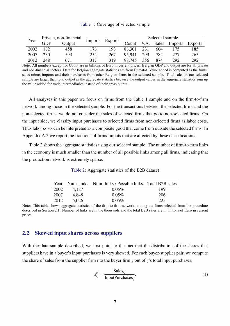
Table 1: Coverage of selected sample
YearPrivate, non-financial
Imports ExportsSelected sample
GDP Output Count V.A. Sales Imports Exports2002 182 458 178 193 88,301 231 604 175 1852007 230 593 254 267 95,941 299 782 277 2652012 248 671 317 319 98,745 356 874 292 292
Note: All numbers except for Count are in billions of Euro in current prices. Belgian GDP and output are for all privateand non-financial sectors. Data for Belgian aggregate statistics are from Eurostat. Value added is computed as the firms’sales minus imports and their purchases from other Belgian firms in the selected sample. Total sales in our selectedsample are larger than total output in the aggregate statistics because the output values in the aggregate statistics sum upthe value added for trade intermediaries instead of their gross output.
All analyses in this paper we focus on firms from the Table 1 sample and on the firm-to-firm
network among those in the selected sample. For the transactions between the selected firms and the
non-selected firms, we do not consider the sales of selected firms that go to non-selected firms. On
the input side, we classify input purchases to selected firms from non-selected firms as labor costs.
Thus labor costs can be interpreted as a composite good that come from outside the selected firms. In
Appendix A.2 we report the fractions of firms’ inputs that are affected by these classifications.
Table 2 shows the aggregate statistics using our selected sample. The number of firm-to-firm links
in the economy is much smaller than the number of all possible links among all firms, indicating that
the production network is extremely sparse.
Table 2: Aggregate statistics of the B2B dataset
Year Num. links Num. links / Possible links Total B2B sales2002 4,187 0.05% 1992007 4,848 0.05% 2062012 5,026 0.05% 225
Note: This table shows aggregate statistics of the firm-to-firm network, among the firms selected from the proceduredescribed in Section 2.1. Number of links are in the thousands and the total B2B sales are in billions of Euro in currentprices.
2.2 Skewed input shares across suppliers
With the data sample described, we first point to the fact that the distribution of the shares that
suppliers have in a buyer’s input purchases is very skewed. For each buyer-supplier pair, we compute
the share of sales from the supplier firm i to the buyer firm j out of j’s total input purchases:
smi j =
Salesi j
InputPurchases j. (1)
7
Input purchases here includes all purchases from other Belgian firms in our sample and imports.
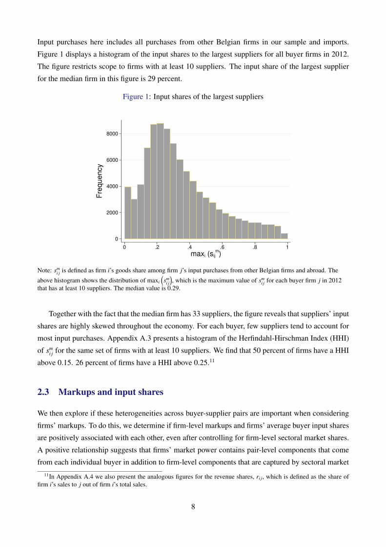
Figure 1 displays a histogram of the input shares to the largest suppliers for all buyer firms in 2012.
The figure restricts scope to firms with at least 10 suppliers. The input share of the largest supplier
for the median firm in this figure is 29 percent.
Figure 1: Input shares of the largest suppliers
0
2000
4000
6000
8000
Fre
qu
en
cy
0 .2 .4 .6 .8 1
maxi (sijm)
Note: smi j is defined as firm i’s goods share among firm j’s input purchases from other Belgian firms and abroad. The
above histogram shows the distribution of maxi
(sm
i j
), which is the maximum value of sm
i j for each buyer firm j in 2012that has at least 10 suppliers. The median value is 0.29.
Together with the fact that the median firm has 33 suppliers, the figure reveals that suppliers’ input
shares are highly skewed throughout the economy. For each buyer, few suppliers tend to account for
most input purchases. Appendix A.3 presents a histogram of the Herfindahl-Hirschman Index (HHI)
of smi j for the same set of firms with at least 10 suppliers. We find that 50 percent of firms have a HHI
above 0.15. 26 percent of firms have a HHI above 0.25.11
2.3 Markups and input shares
We then explore if these heterogeneities across buyer-supplier pairs are important when considering
firms’ markups. To do this, we determine if firm-level markups and firms’ average buyer input shares
are positively associated with each other, even after controlling for firm-level sectoral market shares.
A positive relationship suggests that firms’ market power contains pair-level components that come
from each individual buyer in addition to firm-level components that are captured by sectoral market
11In Appendix A.4 we also present the analogous figures for the revenue shares, ri j, which is defined as the share offirm i’s sales to j out of firm i’s total sales.
8
shares.
Firm-level markups, µi,t, are measured as the ratio of firms’ total sales over variable costs (the
sum of input purchases and labor costs). This measure of firm-level markups is consistent with the
model we construct in Section 3, which is static and features CRS production technologies. As firms
might use additional factors, such as capital inputs, we consider alternative measures of firm-level
markups in Appendix A.7 following De Loecker and Warzynski (2012).12
Firm-level sectoral market shares, SctrMktSharei,t, are computed at the NACE 4-digit level. This
measure captures firms’ market power in models that feature oligopolistic competition where firms’
outputs are aggregated at the sectoral level.
We construct a measure that captures the input shares firms have within their buyers. Using the
pairwise input shares defined in equation (1), we compute firm i’s weighted average input shares to
its buyers at year t, smi·,t, as
smi·,t =
∑j∈Wi,t
InputPurchases j,t∑k∈Wi,t
InputPurchasesk,tsm
i j,t
=
∑j∈Wi,t
Salesi j,t∑j∈Wi,t
InputPurchases j,t,
where Wi,t is the set of i’s buyers at year t. Total input purchases are assigned as weights for each
buyer firm.
With these variables, we run the following regression:
µi,t = βSctrMktSharei,t + γ smi·,t + ϕ Xi,t + δt + εi,t, (2)
where firm-level controls and year fixed effects are included. Table 3 reports the results. The speci-
fication of the first column includes sector fixed effects, and the specifications of the second and the
third columns include firm fixed effects. First, unsurprisingly, in all specifications we see a positive
relationship between markups and firm-level market shares. The result in the third column, for exam-
ple, indicates that within each firm, an increase of one standard deviation in the firm’s market share is
associated with an increase of around 2.2 percentage points in the firm’s markup. More interestingly,
even after controlling for these sectoral market shares, the coefficients on the firms’ average input
shares to buyers are positive. The third column indicates that within each firm a single standard devi-
ation increase in average input shares to buyers leads to around an increase of 3.9 percentage points
in the firm’s markup. Controlling for firms’ size in each sector, firms have greater ability to charge
markups if they have higher shares within their buyers’ inputs.
12We exclude the user cost of capital in the calculation of markups in our baseline case. This is because the firm-to-firmtrade data may capture purchases of capital goods. Adding a measure of user cost of capital leads to double counting ofcapital goods.
9
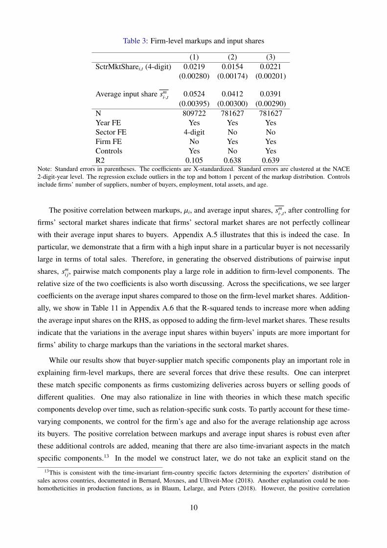
Table 3: Firm-level markups and input shares
(1) (2) (3)SctrMktSharei,t (4-digit) 0.0219 0.0154 0.0221
(0.00280) (0.00174) (0.00201)
Average input share smi·,t 0.0524 0.0412 0.0391
(0.00395) (0.00300) (0.00290)N 809722 781627 781627Year FE Yes Yes YesSector FE 4-digit No NoFirm FE No Yes YesControls Yes No YesR2 0.105 0.638 0.639
Note: Standard errors in parentheses. The coefficients are X-standardized. Standard errors are clustered at the NACE2-digit-year level. The regression exclude outliers in the top and bottom 1 percent of the markup distribution. Controlsinclude firms’ number of suppliers, number of buyers, employment, total assets, and age.
The positive correlation between markups, µi, and average input shares, smi·,t, after controlling for
firms’ sectoral market shares indicate that firms’ sectoral market shares are not perfectly collinear
with their average input shares to buyers. Appendix A.5 illustrates that this is indeed the case. In
particular, we demonstrate that a firm with a high input share in a particular buyer is not necessarily
large in terms of total sales. Therefore, in generating the observed distributions of pairwise input
shares, smi j, pairwise match components play a large role in addition to firm-level components. The
relative size of the two coefficients is also worth discussing. Across the specifications, we see larger
coefficients on the average input shares compared to those on the firm-level market shares. Addition-
ally, we show in Table 11 in Appendix A.6 that the R-squared tends to increase more when adding
the average input shares on the RHS, as opposed to adding the firm-level market shares. These results
indicate that the variations in the average input shares within buyers’ inputs are more important for
firms’ ability to charge markups than the variations in the sectoral market shares.
While our results show that buyer-supplier match specific components play an important role in
explaining firm-level markups, there are several forces that drive these results. One can interpret
these match specific components as firms customizing deliveries across buyers or selling goods of
different qualities. One may also rationalize in line with theories in which these match specific
components develop over time, such as relation-specific sunk costs. To partly account for these time-
varying components, we control for the firm’s age and also for the average relationship age across
its buyers. The positive correlation between markups and average input shares is robust even after
these additional controls are added, meaning that there are also time-invariant aspects in the match
specific components.13 In the model we construct later, we do not take an explicit stand on the
13This is consistent with the time-invariant firm-country specific factors determining the exporters’ distribution ofsales across countries, documented in Bernard, Moxnes, and Ulltveit-Moe (2018). Another explanation could be non-homotheticities in production functions, as in Blaum, Lelarge, and Peters (2018). However, the positive correlation
10
potential sources that drive these components but treat them as pair-specific constant variables in the
production functions, that reflect how suitable goods from each supplier are as inputs for the buyer.
The positive correlation is robust under different average measures of smi·,t, such as taking simple
averages or median values. Furthermore, it is also robust when using other measures of pairwise
input shares. For example, instead of using smi j we use si j, which is the firm i’s sales share in j’s total
variable inputs (input purchases plus labor costs). Another alternative share we use is the supplier’s
sales share among the buyer’s goods inputs that are classified the same as the supplier’s, either at the
2-digit or 4-digit level. We report these results and those of other robustness checks in Appendix A.6.
between markups and average input shares is robust after adding an additional buyer size control variable.
11
3 Model
In the previous section, the Belgian firm-to-firm trade data revealed that firms charge higher markups
when they have higher input shares within their buyers. We interpret this fact as firms competing
as oligopolies to supply inputs to each buyer. In this section, we set up a model of oligopolistic
competition in firm-to-firm trade. Throughout the model we assume a small, open economy, where
we take the foreign price and the foreign demand shifter as given.
3.1 Preference
There is a representative household providing L units of labor. Households have a CES preference
over all firms’ goods with the substitution parameter σ. We assume that firms’ goods are substi-
tutes, thus σ > 1. We also assume that households do not directly consume foreign goods in the
heterogeneous goods sector. The household’s preference is denoted as
U =
∑i∈Ω
βiHqσ−1σ
iH
σσ−1
, (3)
where Ω denotes the set of domestic firms. qiH denotes the quantity of goods that firm i sells to the
household. Given the price that i charges to the household, piH, qiH can be written as
qiH = βσiHp−σiH
P1−σ E, (4)
where E denotes the aggregate expenditure. P denotes the aggregate price index:
P =
∑i∈Ω
βσiH p1−σiH
1
1−σ
. (5)
Demand from abroad is modeled with the same structure as the domestic household. Let IiF be
an indicator of whether firm i is an exporter or not. Given a price that i charges on exported goods,
piF , export quantity, qiF , can be written as
qiF = IiF p−σiF D∗, (6)
where D∗ is the exogenous demand shifter from abroad.
12

3.2 Technology and market structure
Each firm produces a single differentiated good. In addition to labor inputs, they purchase goods from
other firms and/or purchase imported goods as intermediate goods. On the output side, they sell goods
directly to final demand, to other domestic firms, and/or export. We treat firms to be infinitesimal in
the final demand market and assume Dixit and Stiglitz (1977) monopolistic competition. Thus firms
charge constant markups on their goods when selling to the final consumer. We also assume that
firms apply the same markups when exporting.
When considering firm-to-firm trade markets, the assumption of infinitesimal suppliers for each
buyer is not consistent with the data. In Section 2.2, we showed that firms tend to have highly
concentrated input share distributions. A handful of top supplier firms account for the majority of
firms’ goods purchases. Moreover, in Section 2.3, we found that firms charge higher markups when
they have higher input shares to buyers. Therefore, we assume oligopolistic competition in firm-to-
firm trade, where firms charge different markups to different buyers depending on the shares they
have in each buyer’s goods purchases. In doing so, we apply the framework of Atkeson and Burstein
(2008) to firms’ pricing decisions in the relationships with each buyer.
Let Zi be firm i’s set of domestic suppliers and let IFi be the indicator for the importing status of
firm i. We denote i’s sector as u and j’s sector as v. We assume nested CES structures in firms’ pro-
duction functions. A firm first combines domestically supplied goods into sector-level intermediate
goods bundles. Then it combines these sectoral goods and imported goods into a different interme-
diate goods bundle. Finally, the firm combines labor inputs and the intermediate goods bundle to
produce its output. We denote the elasticity of substitution across firms’ goods in sector u as σu. The
substitution parameter across sectoral goods and imported goods is ρ, and the substitution parameter
across labor inputs and the intermediate goods bundle is η. We assume all substitution parameters are
above one.14
The implied unit cost of firm i is
ci = φ−1i
(ωηl w1−η + ωη
m p1−ηmi
) 11−η, (7)
where φi is i’s core productivity. ωl and ωm denote CES weights in the production function on labor
and intermediate goods. w denotes wage, and pmi is the firm-specific price index of intermediate
goods. pmi is another aggregate of firm i’s sector-level domestic intermediate price indices, pmvi, and
the foreign price, pF . pmi and pmvi vary with firms’ sourcing strategy, Zi and IFi, along with the saliency
14We do not impose any restrictions concerning the relative magnitudes among σu, ρ, and η when we estimate themin Section 4.
13
parameters, α ji and αFi:
pmi =
∑v
αρv(pm
vi)1−ρ
+ IFiαρFi p
1−ρF
1
1−ρ
pmvi =
∑j∈Zi, j∈V
ασv( j)
ji p1−σv( j)
ji
1
1−σv( j)
. (8)
V denotes the set of firms in sector v. The term p ji denotes the price that firm j charges for its goods
when selling to firm i. pF is the exogenous price of the foreign good. The terms α ji and αFi reflect
how suitable goods from firm j and foreign imports are as inputs for firm i.
Before discussing the market structures of the final demand market and of the firm-to-firm mar-
kets, we derive the firms’ shares on inputs implied by the above CES structures. The share of firm i’s
variable costs spent on labor, sli, is
sli =ωηl w1−η
c1−ηi φ
1−ηi
. (9)
The intermediate goods’ share, smi, becomes
smi = 1 − sli
=ωηm p1−η
mi
c1−ηi φ
1−ηi
. (10)
Among i’s variable costs spent on intermediate goods, the share of sector v goods, smvi, and the share
of foreign goods, smFi, are, respectively,
smvi = αρv
(pm
vi
)1−ρ
p1−ρmi
,
smFi = IFiα
ρFi
p1−ρF
p1−ρmi
. (11)
Among i’s variable costs spent on sector v goods, the share of firm j’s goods, sv( j)ji , is
sv( j)ji = α
σv( j)
ji
p1−σv( j)
ji(pm
v( j)i
)1−σv( j). (12)
Analogously, we can write s ji and sFi respectively as the shares of j’s goods and foreign goods out of
i’s total variable costs, s ji = sv( j)ji sm
v( j)ismi and sFi = smFismi.
Finally, we turn to the market structures. We assume monopolistic competition when firms sell
to final demand. Firms charge a constant markup over marginal cost, and we assume the same when
14
firms export:
piH = piF =σ
σ − 1ci. (13)
We introduce oligopolistic competition in firm-to-firm trade in the following way. When selling
to firm i, firm j sets price p ji that maximizes variable profits by taking as given prices of i’s other
suppliers and i’s unit cost and output, ci and qi. Solving the firm’s profit maximization problem yields
the following price:
p ji = µ jic j =ε ji
ε ji − 1c j
ε ji = σv( j)
(1 − sv( j)
ji
)+ ρsv( j)
ji
(1 − sm
v( j)i
)+ ηsv( j)
ji smv( j)i. (14)
The price implies that the markup firm j charges on firm i, µ ji, depends on the input shares that j’s
goods have in i’s intermediate goods, sv( j)ji and sm
v( j)i.15 If the supplier j in sector v has an infinitesimally
small share in buyer i’s intermediate goods bundle (sv( j)ji → 0), then all the competition the supplier j
engages in are with the other suppliers in sector v ( j) sharing the same buyer i. The price converges to
the value obtained assuming monopolistic competition, a constant markup of σv( j)
σv( j)−1 . As the supplier’s
input share on the buyer increases, then not only does the supplier compete with the other suppliers,
but also with other suppliers in sectors other than v and the labor input that buyer firm i employs.
Thus, the demand elasticity the supplier faces, ε ji, is a weighted average of σv( j), ρ, and η. These
weights are constructed from the shares sv( j)ji and sm
v( j)i. When the supplier j is the only firm supplying
the buyer (sv( j)ji , s
mv( j)i → 1), the markup converges to η
η−1 . The intuition of how pairwise markups
depend on pairwise shares are identical to what is described in Atkeson and Burstein (2008). The key
difference is that here the relevant shares and markups are defined for each buyer-supplier pair.
As aforementioned, we assume that the supplier takes as given the buyer’s unit cost and output.
This is consistent with the assumption of Bertrand competition, where firms take as given all others’
prices, including the prices of their buyers. A plausible alternative would be to assume that the
supplier firm internalizes the change in demand for the buyer’s good when determining price. In
this case, the supplier needs to know the output composition of the buyer firm to infer the elasticity
of demand the buyer is facing. As firms are unlikely to observe the flow of goods distant in the
production chain, we find our assumption to be reasonable.16
15See Appendix B.1 for firm j’s maximization problem.16The assumption that firms have incomplete information about firms that are distant in the production chain is similar
to that considered by Antras and de Gortari (2017). In Appendix B.2 we discuss in detail the optimal prices that firmscharge their buyers under alternative assumptions. When a firm internalizes the effect of its price on the demand for thebuyer’s goods, the markup it charges not only depends on sv( j)
ji and smv( j)i but also on quantities that the buyer sells to other
firms and the quantities that it sells to final demand. One can also assume that firms take as given a constant demandelasticity buyers are presumed to face. In this case, if one assumes the value of the demand elasticity is η, the pricingequation collapses to that of equation (14). In Appendix B.2 we also discuss optimal prices when firms engage in Cournotcompetition instead of Bertrand competition.
15
This assumption is also consistent with the empirical evidence. Section 2.3 confirmed that firms’
markups are correlated with the firms average input shares within their buyers. We further investigate
if firms’ markups are correlated with the average input shares their buyers have within those buyers’
buyers. We find that the coefficient on these second-degree average input shares is not significant
and close to zero. These results indicate that although firms charge higher markups when possessing
have higher input shares in their buyers, this is not necessarily the case when their buyers have higher
input shares. See Table 19 in Appendix A.6 for details.
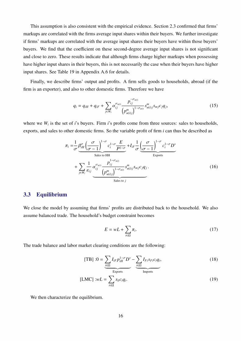
Finally, we describe firms’ output and profits. A firm sells goods to households, abroad (if the
firm is an exporter), and also to other domestic firms. Therefore we have
qi = qiH + qiF +∑j∈Wi
ασu(i)i j
p−σu(i)i j(
pmu(i) j
)1−σu(i)sm
u(i) jsm jc jq j, (15)
where we Wi is the set of i’s buyers. Firm i’s profits come from three sources: sales to households,
exports, and sales to other domestic firms. So the variable profit of firm i can thus be described as
πi =1σβσiH
(σ
σ − 1
)1−σc1−σ
iE
P1−σ︸ ︷︷ ︸Sales to HH
+IiF1σ
(σ
σ − 1
)1−σc1−σ
i D∗︸ ︷︷ ︸Exports
+∑j∈Wi
1εi j
ασu(i)i j
p1−σu(i)i j(
pmu(i) j
)1−σu(i)sm
u(i) jsm jc jq j︸ ︷︷ ︸Sales to j
. (16)
3.3 Equilibrium
We close the model by assuming that firms’ profits are distributed back to the household. We also
assume balanced trade. The household’s budget constraint becomes
E = wL +∑i∈Ω
πi. (17)
The trade balance and labor market clearing conditions are the following:
[TB] :0 =∑i∈Ω
IiF p1−σiH D∗︸ ︷︷ ︸
Exports
−∑i∈Ω
IFisFiciqi︸ ︷︷ ︸Imports
, (18)
[LMC] :wL =∑i∈Ω
sliciqi. (19)
We then characterize the equilibrium.
16
Definition (Equilibrium). Take as given the foreign demand shifter, D∗, and the foreign price, pF .
An equilibrium is a set of variables, w, P, E, qi, that satisfy equations (4)–(19).
Using the system of equations above that defines the equilibrium, in Sections 5 and 6 we solve for
the equilibrium changes in firm-level costs and aggregate welfare, taking the changes in firm-to-firm
markups or the changes in the foreign price as the shock. We implement the technique developed
by Dekle, Eaton, and Kortum (2007), which enables us to compute the counterfactual outcomes with
only shares directly observed in the data,sli, smi, sm
i j, smFi, siH
, and the estimated CES parameters.17
3.4 Alternative models as benchmarks
Before estimating the CES parameters and conducting counterfactual exercises, we provide with
variations of alternative modeling assumptions useful in benchmarking the counterfactual results of
Sections 5 and 6.
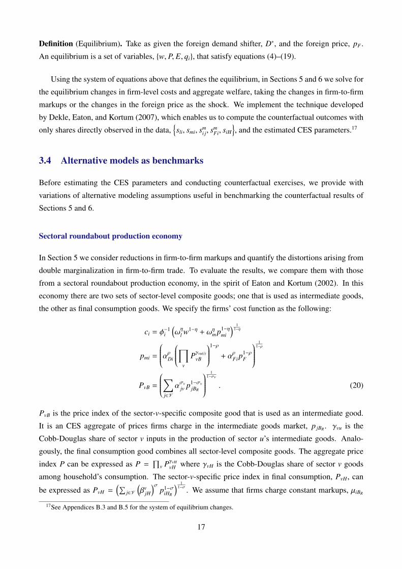
Sectoral roundabout production economy
In Section 5 we consider reductions in firm-to-firm markups and quantify the distortions arising from
double marginalization in firm-to-firm trade. To evaluate the results, we compare them with those
from a sectoral roundabout production economy, in the spirit of Eaton and Kortum (2002). In this
economy there are two sets of sector-level composite goods; one that is used as intermediate goods,
the other as final consumption goods. We specify the firms’ cost function as the following:
ci = φ−1i
(ωηl w1−η + ωη
m p1−ηmi
) 11−η
pmi =
αρDi
∏v
Pγvu(i)vB
1−ρ
+ αρFi p
1−ρF
1
1−ρ
PvB =
∑j∈V
ασvjv p1−σv
jBR
1
1−σv
. (20)
PvB is the price index of the sector-v-specific composite good that is used as an intermediate good.
It is an CES aggregate of prices firms charge in the intermediate goods market, p jBR . γvu is the
Cobb-Douglas share of sector v inputs in the production of sector u’s intermediate goods. Analo-
gously, the final consumption good combines all sector-level composite goods. The aggregate price
index P can be expressed as P =∏
v PγvHvH where γvH is the Cobb-Douglas share of sector v goods
among household’s consumption. The sector-v-specific price index in final consumption, PvH, can
be expressed as PvH =(∑
j∈V
(βv
jH
)σp1−σ
iHR
) 11−σ . We assume that firms charge constant markups, µiBR
17See Appendices B.3 and B.5 for the system of equilibrium changes.
17

and µiHR , to both composite goods for intermediate goods and final consumption, piBR = µiBRci and
piHR = µiHRci. We assume these constant markups to be consistent with the average markups firms
charge on intermediate goods sales and on their sales to final demand in our baseline model.18
This sectoral roundabout production economy is useful as a benchmark because it assumes a sim-
ple network structure while keeping firm-level variables (such as firms’ sales, firms’ inputs, firms’
markups on final demand) and firm-level average markups on intermediate goods sales still consistent
with the data. This roundabout economy has few production layers of intermediate goods, whereas
the real firm-to-firm network features a much more complex production network structure. See Ap-
pendix B.4 for the system of equations solving for the changes in equilibrium variables under this
sectoral roundabout production economy.
Economy with constant markups
In Section 6 we consider changes in the price of foreign goods as the shock and analyze whether
accounting for oligopolistic competition in firm-to-firm trade alters predictions of the transmission of
shocks. To this end, we consider as a benchmark an economy where firms charge constant markups
in firm-to-firm trade. To make the comparison as consistent as possible, we assume firms charge the
same heterogeneous markups that are implied by the baseline economy. However, here we assume
markups are constant and do not change in response to shocks. This alternative model with constant
markups is close to what is considered in Tintelnot, Kikkawa, Mogstad, and Dhyne (2018), but
with sectoral layers in the production functions. We present the system of equations solving for the
changes in equilibrium variables in Appendix B.6.19
18Specifically, we assume µiHR = σσ−1 and µiBR =
∑j pi jqi j
ciqi−piH qiH +piF qiF
µiHR
.19To benchmark the results from Section 6, we additionally consider a back-of-the-envelope calculation of the econ-
omy’s aggregate response under the assumption of perfect competition. Analogous to the argument made by Hulten(1978), with perfect competition and other assumptions, one can solve for the aggregate counterfactual changes usingfirm-level information alone. We outline this approach in Appendix B.7.
18

4 Estimation
The counterfactual exercises using the model setup in the previous section require estimates of the
CES parameters in the preference and production functions, σu , ρ, η, σ, and observables from the
Belgian firm-to-firm trade data. In this section we describe the estimation procedures for the CES
parameters.
We estimate the CES parameters, σu , ρ, η, σ, by exploiting the variations of sales and input
shares at the firm-to-firm level in the data. Recall that in equation (14), pairwise markups, µi j =εi j
εi j−1 ,
are functions of parameters,σu(i)
, ρ, η
, and observable input shares, su(i)
i j and smu(i) j. We have also
assumed markups firms charge on goods sold to domestic households and on exports, µiH, to be σσ−1 .
In our static model, a firm’s total variable input cost — sum of labor costs, purchases from other
firms, and imports, ciqi — has to equal the firm’s total sales, each deflated by destination-specific
markups,∑
jVi j
µi j+ ViH
µiH+ ViF
µiH. Denote the total variable input costs implied from the model as Ci =∑
jVi j
µi j+ ViH
µiH+ ViF
µiH. Respresent the difference between the observed input costs and the model implied
input costs, relative to the observed input costs as
εi =ciqi −Ci
ciqi. (21)
We assume that the accounting identity ciqi = Ci holds in the data up to a measurement error, εi:
Assumption 1. εi are measurement errors and constant variables for each firm.
In the Belgian dataset we observe the input costs, ciqi, firm i’s sales to firm j, Vi j, firm i’s sales to
households, ViH, and firm i’s exports, ViF , for all firms and input shares at the buyer-supplier level, su(i)i j
and smu(i) j. Using these observables, we estimate the CES parameters, σu , ρ, η, σ, by minimizing
the squared sum of the measurement errors, εi:
minσu,ρ,η,σ
∑i
ciqi −Ci
(σu(i)
, ρ, η, σ, su(i)
i j , smu(i) j
)ciqi
2
. (22)
Since firms’ markups to final demand, µiH, are constants of σσ−1 , the variations in the ratio of
firms’ sales to final demand and exports (ViH + ViF) over firms’ total inputs (ciqi) pin down the value
of σ. Firm-to-firm markups, µi j, are functions of pair specific shares, su(i)i j and sm
u(i) j, and parameters,
σu, ρ, and η. Thus the ratio of firm-to-firm sales(Vi j
)over suppliers’ input costs (ciqi), and the input
shares su(i)i j and sm
u(i) j, jointly determine the value of the two parameters.20
We use the categorization of “intermediate SNA/ISIC aggregation A*38” in NACE Rev.2 classi-
20Edmond, Midrigan, and Xu (2015) use a similar procedure with sectoral market shares to infer one of the CESparameters in models with endogenous markups.
19

fication, which leaves us to estimate 29 sectoral substitution parameters of σu and three parameters
of σ, ρ, and η.21 Finally, the model cannot accommodate firms total sales less than their variable
input costs. We drop these firms from the estimation sample, losing around 15 percent of firms that
account for around 28 percent of output. We report the estimation results in Table 4.22
21See European Commission (2008) for details. We aggregate two A*38 codes, CD and CE, into one sector.22To evaluate the sensitivity of estimates to firms in the network, for each sector we draw firm-level samples from the
data with replacements and compute the standard deviations of the estimates from the re-sampled data. However, as thesefirm-level observations are interdependent on the activities of their suppliers and buyers, standard asymptotic propertiesmay not hold with the re-sampled data. See Chandrasekhar (2015) for discussions on conducting inference using networkdata.
20
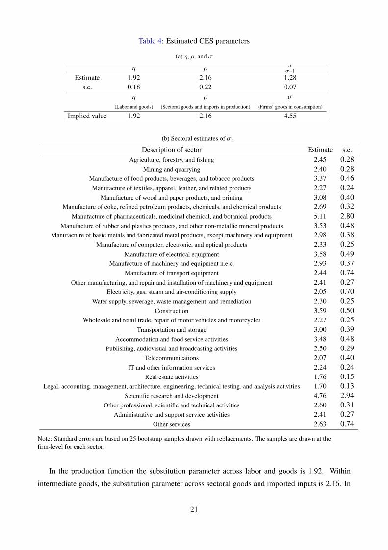
Table 4: Estimated CES parameters
(a) η, ρ, and σ
η ρ σσ−1
Estimate 1.92 2.16 1.28s.e. 0.18 0.22 0.07
η ρ σ
(Labor and goods) (Sectoral goods and imports in production) (Firms’ goods in consumption)
Implied value 1.92 2.16 4.55
(b) Sectoral estimates of σu
Description of sector Estimate s.e.Agriculture, forestry, and fishing 2.45 0.28
Mining and quarrying 2.40 0.28Manufacture of food products, beverages, and tobacco products 3.37 0.46Manufacture of textiles, apparel, leather, and related products 2.27 0.24
Manufacture of wood and paper products, and printing 3.08 0.40Manufacture of coke, refined petroleum products, chemicals, and chemical products 2.69 0.32
Manufacture of pharmaceuticals, medicinal chemical, and botanical products 5.11 2.80Manufacture of rubber and plastics products, and other non-metallic mineral products 3.53 0.48
Manufacture of basic metals and fabricated metal products, except machinery and equipment 2.98 0.38Manufacture of computer, electronic, and optical products 2.33 0.25
Manufacture of electrical equipment 3.58 0.49Manufacture of machinery and equipment n.e.c. 2.93 0.37
Manufacture of transport equipment 2.44 0.74Other manufacturing, and repair and installation of machinery and equipment 2.41 0.27
Electricity, gas, steam and air-conditioning supply 2.05 0.70Water supply, sewerage, waste management, and remediation 2.30 0.25
Construction 3.59 0.50Wholesale and retail trade, repair of motor vehicles and motorcycles 2.27 0.25
Transportation and storage 3.00 0.39Accommodation and food service activities 3.48 0.48
Publishing, audiovisual and broadcasting activities 2.50 0.29Telecommunications 2.07 0.40
IT and other information services 2.24 0.24Real estate activities 1.76 0.15
Legal, accounting, management, architecture, engineering, technical testing, and analysis activities 1.70 0.13Scientific research and development 4.76 2.94
Other professional, scientific and technical activities 2.60 0.31Administrative and support service activities 2.41 0.27
Other services 2.63 0.74
Note: Standard errors are based on 25 bootstrap samples drawn with replacements. The samples are drawn at thefirm-level for each sector.
In the production function the substitution parameter across labor and goods is 1.92. Within
intermediate goods, the substitution parameter across sectoral goods and imported inputs is 2.16. In
21
the preference function, the substitution parameter across goods is 4.55. The estimated values fall in
ranges not far from the findings of different approaches. Chan (2017) finds labor and intermediates
to be gross substitutes. The survey of Anderson and van Wincoop (2004) finds that, within sectors,
the elasticity of substitution across goods in the production function ranges from around 5 to 10
depending on the aggregation. Our estimates of σu are slightly lower than this because our estimates
pick up the substitutability of firms goods among the small set of suppliers that firms source from in
each sector instead of the substitutability of goods among all firms in each sector.23
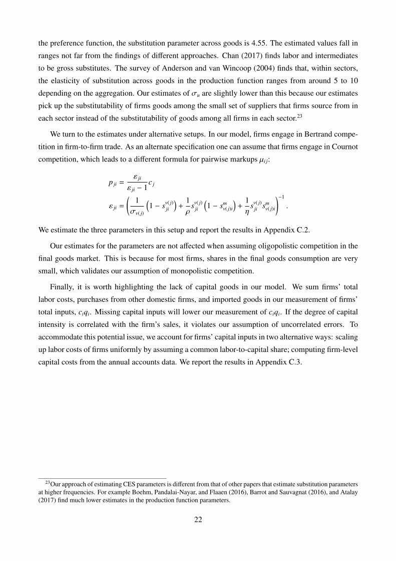
We turn to the estimates under alternative setups. In our model, firms engage in Bertrand compe-
tition in firm-to-firm trade. As an alternate specification one can assume that firms engage in Cournot
competition, which leads to a different formula for pairwise markups µi j:
p ji =ε ji
ε ji − 1c j
ε ji =
(1
σv( j)
(1 − sv( j)
ji
)+
1ρ
sv( j)ji
(1 − sm
v( j)i
)+
1η
sv( j)ji sm
v( j)i
)−1
.
We estimate the three parameters in this setup and report the results in Appendix C.2.
Our estimates for the parameters are not affected when assuming oligopolistic competition in the
final goods market. This is because for most firms, shares in the final goods consumption are very
small, which validates our assumption of monopolistic competition.
Finally, it is worth highlighting the lack of capital goods in our model. We sum firms’ total
labor costs, purchases from other domestic firms, and imported goods in our measurement of firms’
total inputs, ciqi. Missing capital inputs will lower our measurement of ciqi. If the degree of capital
intensity is correlated with the firm’s sales, it violates our assumption of uncorrelated errors. To
accommodate this potential issue, we account for firms’ capital inputs in two alternative ways: scaling
up labor costs of firms uniformly by assuming a common labor-to-capital share; computing firm-level
capital costs from the annual accounts data. We report the results in Appendix C.3.
23Our approach of estimating CES parameters is different from that of other papers that estimate substitution parametersat higher frequencies. For example Boehm, Pandalai-Nayar, and Flaaen (2016), Barrot and Sauvagnat (2016), and Atalay(2017) find much lower estimates in the production function parameters.
22
5 How distortionary are markups in firm-to-firm trade?
With the estimated parameters, in this section we explore how distortionary markups in firm-to-firm
trade are. The observed input shares at the buyer-supplier level, sv( j)ji and sm
v( j)i, and the CES parameters
enable us to back-out the pair-specific markups implied by the model (see equation (14)). We consider
a reduction in those markups in firm-to-firm trade, µi j, as the shock.
Because firms’ outputs pass through many other firms until reaching final demand, the effect of
a reduction in a markup that firm i charges to firm j, µi j, will be amplified when firm j reduces
markups to its buyers. We feed in the shock of µi j, where µi j is the markup backed-out from the data,
and consider the following system of counterfactual changes:
c1−ηi =sliw1−η + smi p
1−ηmi
p1−ρmi =
∑v
smvi(pm
vi)1−ρ
+ smFi(
pmvi)1−σv =
∑j∈Zi, j∈V
sv( j)ji µ
1−σvji c1−σv( j)
j
Ci =1Ci
ViH
µiHsiH E +
1Ci
ViF
µiHViF +
1Ci
∑j
Vi j si j
µi jµi jC j
E =1
1 −∑
i1EµiH−1µiH
ViH siH
wLE
w +∑
i
πi
E
∑k
1πi
Vikµikµik − 1µikµik
sikCk +1πi
µiH − 1µiH
ViFViF
w =
1wL
∑i
sliciqi sliCi. (23)
Ci denotes the total input values of firm i implied by the model: Ci =∑
jVi j
µi j+ ViH
µiH+ ViF
µiH. Furthermore,
sv( j)ji = µ
1−σv( j)
ji c1−σv( j)
j
(pm
v( j)i
)σv( j)−1, sm
vi =(pm
vi
)1−ρpρ−1
mi , smi = p1−ηmi cη−1
i , s ji = sv( j)ji sm
v( j)i smi, sli = w1−ηcη−1i ,
siH = c1−σi Pσ−1, P1−σ =
∑i siH c1−σ
i , ViF = c1−σi .
Taking the data into the system above reveals that firms’ total input values implied by the model,
Ci, do not necessary match the observed input values, ciqi. While we minimized the difference
between the two when estimating the CES parameters, the model under the estimated parameters
is still not entirely consistent with the data. For some firms the observed inputs, ciqi, are larger
than the model implied values, Ci. For other firms, the observed input values seem lower than is
necessary to produce what is sold. To be consistent with the estimation strategy, in the counterfactual
analyses we take the error term in equation (21), εi =ciqi−Ci
ciqi, as constants. We designate ξi as the
difference between the observed input values and model implied input values, ξi = ciqi − Ci. With
this assumption, the changes in the observed inputs, ciqi∧
, are equal to the changes in the model
implied inputs, Ci, and are also equal to the changes in the difference between the two, ξi. One
may alternatively take the values of ξi as constant numbers, and solve for both ciqi∧
and Ci using the
23
relationship ciqi∧
= Ciciqi
Ci +ξi
ciqi. However, for firms with negative values of ξi and under extreme cases
where the values of Ci are low, ciqi∧
can become negative and not well defined. We treat the observed
trade balance as fixed in the counterfactual analyses. We outline the detailed steps solving the system
of counterfactual changes in Appendix B.3.
To evaluate the results, we contrast them with the results from the sectoral roundabout production
economy described in Section 3.4. The sectoral roundabout production economy imposes a particular
structure on the production network. There are two distinct composite goods, one of which is used
as intermediate goods and the another is used as a final consumption good. The sectoral roundabout
production economy does not match the observed firm-to-firm transactions but matches the firm-level
exports, imports, domestic sales, labor costs, domestic purchases, value added, markups charged to
final demand sales, and firm-level average markups charged to sales to intermediate goods. Therefore,
this comparison with the roundabout production economy is useful for evaluating the implications of
markup distortions that account for the real firm-to-firm network. We consider the reduction in the
markups firms charge to the composite good used as intermediate goods as the shock. We outline the
system of counterfactual changes under the sectoral roundabout production economy in Appendix
B.4.
We focus on a 20 percent reduction in markups under the two models.24 That is, we feed in
the shock of µi j =(µi j−1)×0.8+1
µi jfor the baseline economy and µiBR =
(µiBR−1)×0.8+1µiBR
for the sectoral
roundabout production economy. We present the results of firm-level cost changes under the two
economies in Figure 2. In both economies the cost changes are bounded from above by the increases
in the nominal wage, w, which are 4.2 percent in the baseline economy and 4.4 percent in the sec-
toral roundabout production economy. While there is a large heterogeneity in the cost changes under
the baseline economy, the cost changes under the sectoral roundabout production economy are more
compressed. In the baseline economy some firms’ costs decrease by up to 37 percent, the largest de-
cline in firm-level costs in the sectoral roundabout production economy is only by 14 percent. This is
because the sectoral roundabout production economy cannot capture the within sector heterogeneities
in firms’ exposure to other firms’ goods.
24We present results for the other magnitudes of markup reductions in Appendix D.3.
24
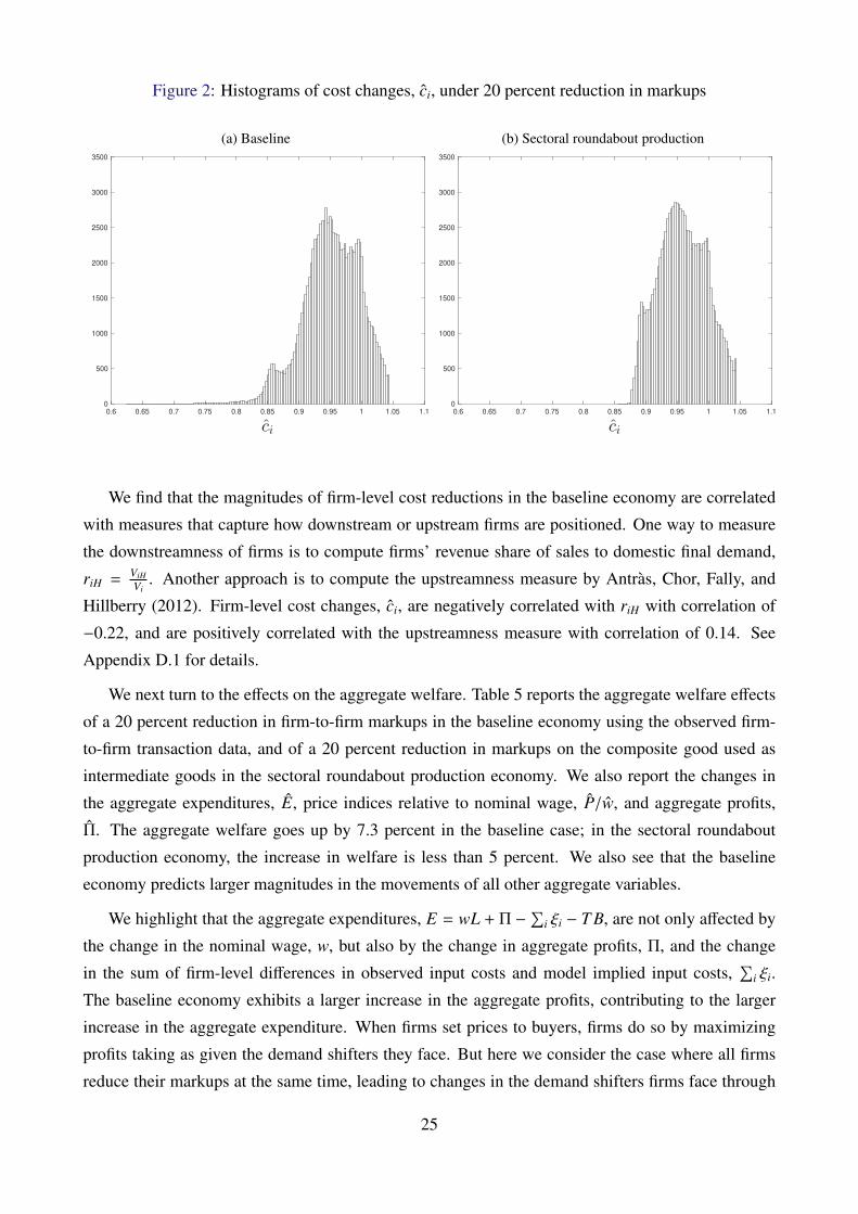
Figure 2: Histograms of cost changes, ci, under 20 percent reduction in markups
(a) Baseline
0.6 0.65 0.7 0.75 0.8 0.85 0.9 0.95 1 1.05 1.1
0
500
1000
1500
2000
2500
3000
3500
(b) Sectoral roundabout production
0.6 0.65 0.7 0.75 0.8 0.85 0.9 0.95 1 1.05 1.1
0
500
1000
1500
2000
2500
3000
3500
We find that the magnitudes of firm-level cost reductions in the baseline economy are correlated
with measures that capture how downstream or upstream firms are positioned. One way to measure
the downstreamness of firms is to compute firms’ revenue share of sales to domestic final demand,
riH = ViHVi
. Another approach is to compute the upstreamness measure by Antras, Chor, Fally, and
Hillberry (2012). Firm-level cost changes, ci, are negatively correlated with riH with correlation of
−0.22, and are positively correlated with the upstreamness measure with correlation of 0.14. See
Appendix D.1 for details.
We next turn to the effects on the aggregate welfare. Table 5 reports the aggregate welfare effects
of a 20 percent reduction in firm-to-firm markups in the baseline economy using the observed firm-
to-firm transaction data, and of a 20 percent reduction in markups on the composite good used as
intermediate goods in the sectoral roundabout production economy. We also report the changes in
the aggregate expenditures, E, price indices relative to nominal wage, P/w, and aggregate profits,
Π. The aggregate welfare goes up by 7.3 percent in the baseline case; in the sectoral roundabout
production economy, the increase in welfare is less than 5 percent. We also see that the baseline
economy predicts larger magnitudes in the movements of all other aggregate variables.
We highlight that the aggregate expenditures, E = wL + Π −∑
i ξi − T B, are not only affected by
the change in the nominal wage, w, but also by the change in aggregate profits, Π, and the change
in the sum of firm-level differences in observed input costs and model implied input costs,∑
i ξi.
The baseline economy exhibits a larger increase in the aggregate profits, contributing to the larger
increase in the aggregate expenditure. When firms set prices to buyers, firms do so by maximizing
profits taking as given the demand shifters they face. But here we consider the case where all firms
reduce their markups at the same time, leading to changes in the demand shifters firms face through
25

the general equilibrium. In the observed firm-to-firm network, firms’ outputs go through multiple
firms until final demand, resulting in larger magnitudes of these general equilibrium effects. On
the other hand, in the sectoral roundabout production economy all firms’ output reach final demand
through a layer of the composite goods, resulting in smaller magnitudes of changes in the demand
shifters.
In addition to these changes in profits, as markups go down and firms use greater amount of inputs,
the differences in observed input costs and model implied input costs,∑
i ξi, become larger as well.
This stems from the assumption that we keep the firm-level ratio of εi = ξi/ciqi fixed instead of the
values of the differences, ξi. In both the baseline economy and in the sectoral roundabout economy,
the total differences,∑
i ξi, increase by 31 percent. These increases in∑
i ξi move in the direction
that will decrease the aggregate expenditures, E. Therefore we interpret the 2.1 percent increase in
the aggregate expenditure as a conservative estimate. In order to only take into account the effects
of the changes in the nominal wage and the aggregate profits on the changes in aggregate welfare,
in Appendix D.2 we present results on the aggregate changes from three different approaches. First,
we compute the changes in aggregate welfare without considering the change in∑
i ξi. We define E
as wL + Π − T B and present the aggregate changes that come from the changes in E. Second, we
present counterfactual results in which we treat ξi as fixed instead of treating εi as fixed.25 Third,
we follow the approach by Ossa (2014) and first eliminate the differences between the observed and
model implied input values, ξi. We solve for the counterfactual changes by forcing the observed
differences, ξi, to zero. The resulting economy becomes fully consistent with the model, with which
we can solve for the counterfactual changes under µi j. In all three approaches aggregate expenditure,
E, increases by larger amounts.
Table 5: Aggregate effects of a 20 percent reduction in markups
Baseline Sectoral roundaboutU = E/P 1.073 1.049
E 1.021 1.010P/w 0.913 0.920Π 1.100 1.079
Note: In the baseline case we take the baseline model using the observed firm-to-firm trade network in 2012. We feed a20 percent reduction in all markups in firm-to-firm trade as the shock, µi j =
(µi j−1)×0.8+1µi j
. In the roundabout productioncase we take the roundabout production economy using the observed firm-level sales and inputs in 2012. We feed a 20
percent reduction in all markups charged to the composite good used as intermediate goods, µiBR =(µiBR−1)×0.8+1
µiBR.
It is worthwhile to put these numbers in context with other papers in the literature. Baqaee
and Farhi (2018) use firm-level data with sectoral Input-Output data from the U.S. and find that
eliminating firm-level markups would lead to an increase in the TFP by around 20 percent at the
25As mentioned on page 24, this approach cannot accommodate extreme cases.
26

second-order approximation. Instead of taking first-order or second-order approximations, we impose
a particular structure on how markups are determined at the firm-to-firm level, and compute the
welfare benefits of reducing those markups. Although these numbers are not directly comparable,
one reason we predict large aggregate effects is that the markups we back out are generally higher
in firm-to-firm trade than in firms’ sales to final demand. With our estimates of the CES parameters,
our model indicates that while firms charge markups of 1.28 in their sales to final demand, firms on
average charge markups of around 1.62 to other firms.26 Instead of assuming firm-level markups that
are common across destinations, we incorporate these differences and consider reductions in markups
that are initially at higher levels.
Another reason relates to the greater effects of our baseline economy compared to the sectoral
roundabout production economy. Considering the observed firm-to-firm network generates substan-
tial heterogeneity in firm-level cost changes, and there are a few firms that experience extreme cost
reductions.27 Due to non-linearities in the system of equilibrium changes (23), firms with large cost
reductions obtain larger shares in both the final demand market and among their buyers’ inputs, which
leads to greater movements in the aggregate. As we saw in Figure 2, the sectoral roundabout produc-
tion economy fails to capture large heterogeneity in firm-level cost changes. In Appendix D.3 we also
consider the system of first-order approximated equilibrium changes and illustrate the non-linearities
of the system by analyzing different magnitudes of shocks. We find that under first-order approxi-
mation, eliminating all firm-to-firm markups would lead to a 30 percent approximate increase in the
aggregate welfare.
26The level of these accounting markups are generally higher than other estimates of markups for Belgium (see forexample De Loecker et al., 2018). This is primarily because our measure of accounting markups only take into accountimports, labor costs, and inputs from other firms as production costs, and exclude other costs such as capital usage costs.
27Because of this subset of firms that experience extreme cost reductions, we cannot compute counterfactual changesupon shocks of magnitudes larger than 50 percent reduction in markups. Beyond this point, there are firms with ci soclose to zero that a numerical solution is not obtained.
27
6 How do markups in firm-to-firm trade alter predictions of the
transmission of shocks?
In the previous section, we backed out markups at the buyer-supplier level and took the reduction
of these markups as the exogenous shock. The exercise informed us of the magnitude of distortions
that are present due to double marginalization in the observed firm-to-firm network. Another point of
interest is the treatment of these markups as endogenous variables and the investigation of how these
endogenous markups in firm-to-firm trade alter predictions of transmission shocks.
In this section we take the exogenous parameter of the model, the price of foreign goods, pF , and
use its changes as the shock. Similar to the approaches taken in the previous section, we take as given
the change in foreign price, pF , and consider the system of counterfactual changes presented below:
c1−ηi =sliw1−η + smi p
1−ηmi
p1−ρmi =
∑v
smvi(pm
vi)1−ρ
+ smFi p
1−ρF(
pmvi)1−σv =
∑j∈Zi, j∈V
sv( j)ji µ
1−σvji c1−σv
j
µ ji =ε jiε ji − 1ε jiε ji − 1
Ci =1Ci
ViH
µiHsiH E +
1Ci
ViF
µiHViF +
1Ci
∑j
Vi j si j
µi jµi jC j
E =1
1 −∑
i1EµiH−1µiH
ViH siH
wLE
w +∑
i
πi
E
∑k
1πi
Vikµikµik − 1µikµik
sikCk +1πi
µiH − 1µiH
ViFViF
w =
1wL
∑i
sliciqi sliCi. (24)
Furthermore, ε jiε ji = σv( j)
(1 − sv( j)
ji sv( j)ji
)+ ρsv( j)
ji sv( j)ji
(1 − sm
v( j)i smv( j)i
)+ ηsv( j)
ji smv( j)i s
v( j)ji sm
v( j)i,
sv( j)ji = µ
1−σv( j)
ji c1−σv( j)
j
(pm
v( j)i
)σv( j)−1, sm
vi =(pm
vi
)1−ρpρ−1
mi , smi = p1−ηmi cη−1
i , sli = w1−ηcη−1i , P1−σ =
∑i siH c1−σ
i ,
siH = c1−σi Pσ−1, and ViF = c1−σ
i . The above system is different from the system presented in (23) in
that we now have the shock pF in the second equation and that the changes in firm-to-firm markups,
µi j, are additional endogenous variables to solve for. As in the previous section, we treat the error
terms in equation (21), εi =ξi
ciqi, and observed trade balance as constants.
We focus on a 20 percent reduction in the foreign price as the shock, pF = 0.8, and analyze its
firm-level and aggregate consequences.28 We compare these results with those from the alternative
model of constant markups laid out in Section 3.4.
We plot the histogram of firm-level cost changes under the above system in Figure 3a. Nominal
28We present results for the other magnitudes of foreign price reductions in Appendix E.5.
28
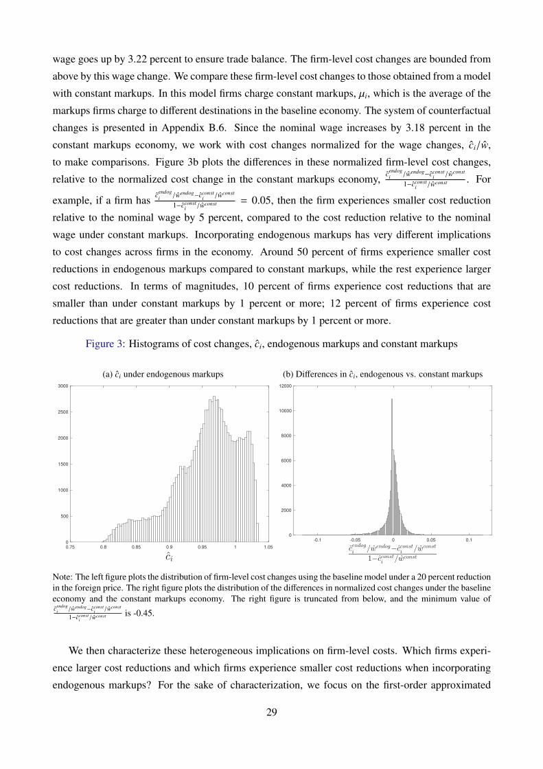
wage goes up by 3.22 percent to ensure trade balance. The firm-level cost changes are bounded from
above by this wage change. We compare these firm-level cost changes to those obtained from a model
with constant markups. In this model firms charge constant markups, µi, which is the average of the
markups firms charge to different destinations in the baseline economy. The system of counterfactual
changes is presented in Appendix B.6. Since the nominal wage increases by 3.18 percent in the
constant markups economy, we work with cost changes normalized for the wage changes, ci/w,
to make comparisons. Figure 3b plots the differences in these normalized firm-level cost changes,
relative to the normalized cost change in the constant markups economy, cendogi /wendog−cconst
i /wconst
1−cconsti /wconst . For
example, if a firm has cendogi /wendog−cconst
i /wconst
1−cconsti /wconst = 0.05, then the firm experiences smaller cost reduction
relative to the nominal wage by 5 percent, compared to the cost reduction relative to the nominal
wage under constant markups. Incorporating endogenous markups has very different implications
to cost changes across firms in the economy. Around 50 percent of firms experience smaller cost
reductions in endogenous markups compared to constant markups, while the rest experience larger
cost reductions. In terms of magnitudes, 10 percent of firms experience cost reductions that are
smaller than under constant markups by 1 percent or more; 12 percent of firms experience cost
reductions that are greater than under constant markups by 1 percent or more.
Figure 3: Histograms of cost changes, ci, endogenous markups and constant markups
(a) ci under endogenous markups
0.75 0.8 0.85 0.9 0.95 1 1.05
0
500
1000
1500
2000
2500
3000
(b) Differences in ci, endogenous vs. constant markups
-0.1 -0.05 0 0.05 0.1
0
2000
4000
6000
8000
10000
12000
Note: The left figure plots the distribution of firm-level cost changes using the baseline model under a 20 percent reductionin the foreign price. The right figure plots the distribution of the differences in normalized cost changes under the baselineeconomy and the constant markups economy. The right figure is truncated from below, and the minimum value ofcendog
i /wendog−cconsti /wconst
1−cconsti /wconst is -0.45.
We then characterize these heterogeneous implications on firm-level costs. Which firms experi-
ence larger cost reductions and which firms experience smaller cost reductions when incorporating
endogenous markups? For the sake of characterization, we focus on the first-order approximated
29
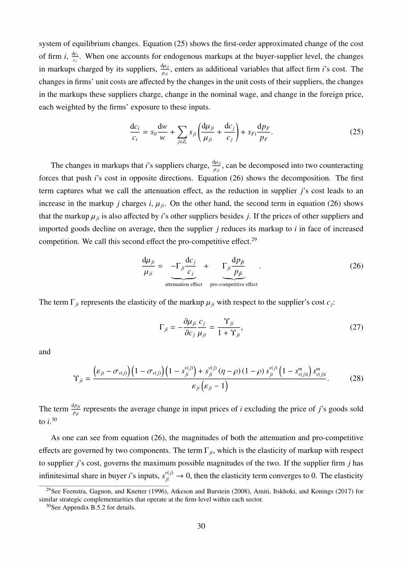
system of equilibrium changes. Equation (25) shows the first-order approximated change of the cost
of firm i, dcici
. When one accounts for endogenous markups at the buyer-supplier level, the changes
in markups charged by its suppliers, dµ ji
µ ji, enters as additional variables that affect firm i’s cost. The
changes in firms’ unit costs are affected by the changes in the unit costs of their suppliers, the changes
in the markups these suppliers charge, change in the nominal wage, and change in the foreign price,
each weighted by the firms’ exposure to these inputs.
dci
ci= sli
dww
+∑j∈Zi
s ji
(dµ ji
µ ji+
dc j
c j
)+ sFi
dpF
pF. (25)
The changes in markups that i’s suppliers charge, dµ ji
µ ji, can be decomposed into two counteracting
forces that push i’s cost in opposite directions. Equation (26) shows the decomposition. The first
term captures what we call the attenuation effect, as the reduction in supplier j’s cost leads to an
increase in the markup j charges i, µ ji. On the other hand, the second term in equation (26) shows
that the markup µ ji is also affected by i’s other suppliers besides j. If the prices of other suppliers and
imported goods decline on average, then the supplier j reduces its markup to i in face of increased
competition. We call this second effect the pro-competitive effect.29
dµ ji
µ ji= −Γ ji
dc j
c j︸ ︷︷ ︸attenuation effect
+ Γ jidp6 jip6 ji︸ ︷︷ ︸
pro-competitive effect
. (26)
The term Γ ji represents the elasticity of the markup µ ji with respect to the supplier’s cost c j:
Γ ji = −∂µ ji
∂c j
c j
µ ji=
Υ ji
1 + Υ ji, (27)
and
Υ ji =
(ε ji − σv( j)
) (1 − σv( j)
) (1 − sv( j)
ji
)+ sv( j)
ji (η − ρ) (1 − ρ) sv( j)ji
(1 − sm
v( j)i
)sm
v( j)i
ε ji
(ε ji − 1
) . (28)
The term dp6 jip6 ji
represents the average change in input prices of i excluding the price of j’s goods sold
to i.30
As one can see from equation (26), the magnitudes of both the attenuation and pro-competitive
effects are governed by two components. The term Γ ji, which is the elasticity of markup with respect
to supplier j’s cost, governs the maximum possible magnitudes of the two. If the supplier firm j has
infinitesimal share in buyer i’s inputs, sv( j)ji → 0, then the elasticity term converges to 0. The elasticity
29See Feenstra, Gagnon, and Knetter (1996), Atkeson and Burstein (2008), Amiti, Itskhoki, and Konings (2017) forsimilar strategic complementarities that operate at the firm-level within each sector.
30See Appendix B.5.2 for details.
30
term also converges to 0 when the supplier firm j is the only supplier of buyer i, sv( j)ji , s
mv( j)i → 1.
Hence both attenuation and pro-competitive effects can have large magnitudes when the pair-specific
input shares are in the intermediate range. This point can be conveyed visually when we collapse
the model to a single-sector model. Once we assume σu = ρ, then the relevant input share that
determines the markup becomes smji = sv( j)
ji smv( j)i from equation (14), and equation (28) collapses to
Υ ji =(ε ji−ρ)(1−ρ)
(1−sm
ji
)ε ji(ε ji−1) . Figure 4 plots markups, µ ji, and the elasticity of markups, Γ ji, with respect to
the input share, smji. One can see that Γ ji displays a hump shape with respect to the input share, sm
ji,
and when the input share is around 0.7, both attenuation and pro-competitive effects can have large
magnitudes.
Figure 4: Markup µ ji and elasticity Γ ji with respect to input share smji, single-sector model
0 0.5 1
1
1.5
2
2.5
0 0.5 1
0
0.05
0.1
0.15
0.2
0.25
Note: The left figure plots the pairwise markup, µ ji, as a function of smji. The right figure plots the elasticity of µ ji with
respect to c j, Γ ji, as a function of smji. For illustration we impose a single-sector structure, σu = ρ. We use the parameter
values of ρ = 2.16 and η = 1.92.
In addition to the elasticity term Γ ji, the magnitudes of the attenuation and pro-competitive effects
are each influenced by how much shock the supplier or other suppliers received, dc j
c jand dp6 ji
p6 ji, respec-
tively. For example, even if the input share for a specific pair is in the region where the elasticity Γ ji
is large, if the supplier’s cost did not decrease at all, there will be no attenuation effect. The mag-
nitudes of cost reductions by the suppliers govern the magnitudes of attenuation effects within the
same values of input shares. Likewise, the average magnitudes of price changes by other suppliers
determine the magnitudes of pro-competitive effects within the same value of input shares. Further-
more, the markup that the supplier j charges i would see net decrease if supplier j’s cost reduction is
greater than the average cost reductions of other suppliers. It would see net increase if other suppliers
received greater cost reductions than what j received.
Having characterized the changes in markups at the buyer-supplier level, we move our attention
to firm-level changes in average markups. As seen in equation (25), the additional force that affects
firm i’s costs by taking into account endogenous markups can be summarized by the average change
31
in markups that suppliers charge to firm i,∑
j∈Zis ji
dµ ji
µ ji. As discussed above, these changes in markups
are governed by the input shares suppliers have and the relative magnitudes of the suppliers’ cost
changes to the other suppliers’ cost changes. Suppose that firm i has multiple suppliers. The largest
supplier, j, with input shares sv( j)ji and sm
v( j)i which predict a large markup elasticity, Γ ji, receives the
largest cost reduction among i’s suppliers. Then the supplier j will increase its markup, and i will
experience higher markups from its suppliers on average. If, on the other hand, j does not experience
any cost reduction while other suppliers do, then j will reduce its markup and i will experience lower
markups from its suppliers on average.
To approximate these firm-level changes in average markups, we consider a measure that captures
firms’ indirect exposure to foreign inputs, sIndirectFi . We first construct the measure of “total foreign
input share,” sTotalFi , that captures firm i’s exposure to foreign inputs by summing its direct exposure,
its suppliers’ exposure, and so on:31
sTotalFi = sFi +
∑k∈Zi
skisTotalFk .
We then subtract firms’ direct exposure to foreign inputs: sIndirectFi = sTotal
Fi − sFi. Figure 5 plots these
average changes in suppliers’ markups,∑
j∈Zis ji
dµ ji
µ ji, against firms’ indirect exposure to foreign inputs,
sIndirectFi . There is a positive correlation between the two measures. Consider a firm with high value of
sIndirectFi , meaning that the supplier with a high input share is highly exposed to foreign imports. In this
case the supplier with the high input share increases its markup and the firm will experience higher
markups on average. This positive correlation informs us that the firm’s position in its production
network is an important determinant of whether the firm experiences greater or smaller cost changes
than those implied from models with constant markups.
To confirm this point, we present the correlations of firm-level cost changes and firm-level vari-
ables in Appendix E.1. The measure of the total foreign input share, sTotalFi , has the largest correlation
with the cost changes under endogenous markups among other firm-level variables such as total
sales, import share, and the number of suppliers. Even so, the measure of indirect foreign input
share, sIndirectFi , predicts best the differences in cost changes under endogenous markups and constant
markups, cendogi /wendog−cconst
i /wconst
1−cconsti /wconst .
31We follow the definition of sTotalFi by Tintelnot, Kikkawa, Mogstad, and Dhyne (2018).
32

Figure 5: Average change in markups,∑
j∈Zis ji
dµ ji
µ ji, and indirect exposure to foreign inputs, sIndirect
Fi
Note: The figure plots the first-order approximated changes in average markups charged by suppliers,∑
j∈Zis ji
dµ ji
µ ji, on a
20 percent reduction in the price of foreign goods, against firms’ indirect exposure to foreign goods, sIndirectFi . The
least-squares line has a y-intercept of -0.0002 and slope coefficient of 0.0009. The R-squared is 0.15. The correlationbetween the two variables is 0.39.
In addition to the firms’ position in the production network, the nature of the shock itself also
affects how firms’ cost changes behave differently from those under constant markups. The shock we
focus on here affects all importers (accounting for around 20 percent of all firms) directly, and many
other firms indirectly at the same time. The median value of the total foreign input share, sTotalFi , is
around 39 percent. As the shock affects many firms in the economy at the same time, many firms
have multiple suppliers which experience roughly the same degree of cost reductions. In these cases,
both the attenuation effects and the pro-competitive effects tend to cancel each other out. To illustrate
this point, in Appendix E.2 we study an alternative shock where we hit only one importer with the
foreign price reduction.32 We demonstrate that the positive correlation between the average changes
in markups,∑
j∈Zis ji
dµ ji
µ ji, and firms’ exposure to the firm’s goods is much stronger. Moreover, we
show that the differences in firm-level cost changes between the baseline model and under constant
markups become greater. In this case, 71 percent of firms experience cost reductions that are smaller
than under constant markups by 1 percent or more, and 9 percent of firms experience cost reductions
that are greater than under constant markups by 1 percent or more.
Finally, we turn to the aggregate counterfactual changes. We report in Table 6 the counterfactual
changes of aggregate welfare, expenditure, price index relative to nominal wage, and profits across the
32We choose the importer with the largest number of domestic buyer as the firm receiving the shock.
33
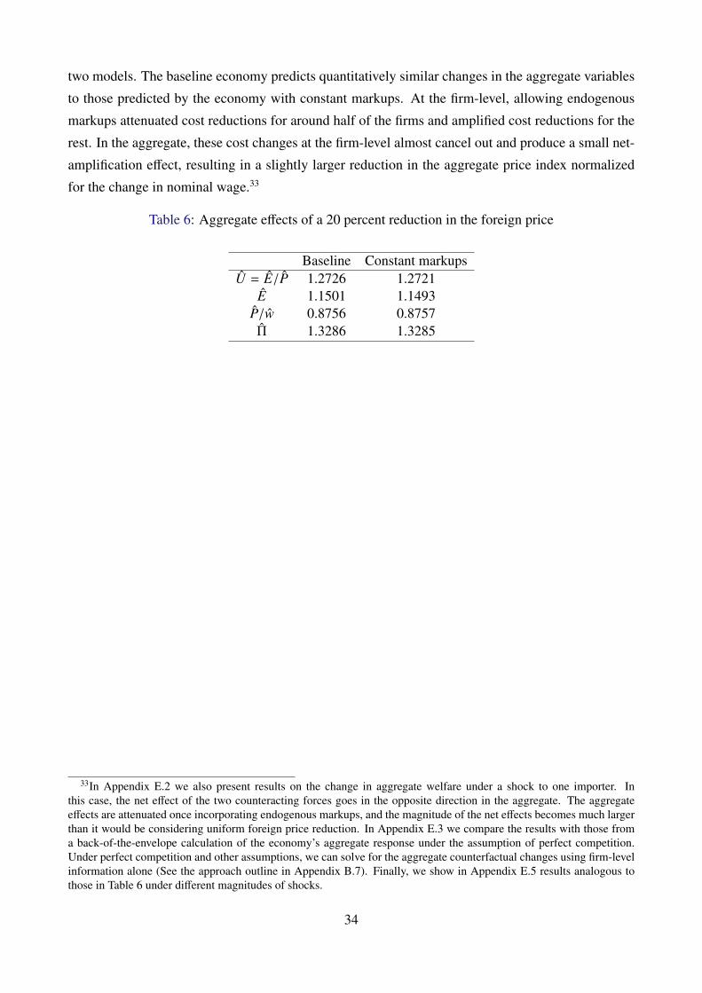
two models. The baseline economy predicts quantitatively similar changes in the aggregate variables
to those predicted by the economy with constant markups. At the firm-level, allowing endogenous
markups attenuated cost reductions for around half of the firms and amplified cost reductions for the
rest. In the aggregate, these cost changes at the firm-level almost cancel out and produce a small net-
amplification effect, resulting in a slightly larger reduction in the aggregate price index normalized
for the change in nominal wage.33
Table 6: Aggregate effects of a 20 percent reduction in the foreign price
Baseline Constant markupsU = E/P 1.2726 1.2721
E 1.1501 1.1493P/w 0.8756 0.8757Π 1.3286 1.3285
33In Appendix E.2 we also present results on the change in aggregate welfare under a shock to one importer. Inthis case, the net effect of the two counteracting forces goes in the opposite direction in the aggregate. The aggregateeffects are attenuated once incorporating endogenous markups, and the magnitude of the net effects becomes much largerthan it would be considering uniform foreign price reduction. In Appendix E.3 we compare the results with those froma back-of-the-envelope calculation of the economy’s aggregate response under the assumption of perfect competition.Under perfect competition and other assumptions, we can solve for the aggregate counterfactual changes using firm-levelinformation alone (See the approach outline in Appendix B.7). Finally, we show in Appendix E.5 results analogous tothose in Table 6 under different magnitudes of shocks.
34

7 Conclusion
In this paper we studied the implications of imperfect competition in firm-to-firm trade. We proposed
a novel view on competition between firms. In addition to the market shares within sectors deter-
mining firms’ market power, we suggest that the relative size of the firm in the total input sourcing
of its buyers is also a relevant metric. The data on firm-to-firm transactions supports this view; firms
charge higher markups if they have higher average input shares within their buyer firms, controlling
for their sectoral market shares.
Using a model of oligopolistic competition in firm-to-firm trade where firms charge different
markups to different buyers, we offered two counterfactual exercises. We first investigated the amount
of distortion caused by variable markups in firm-to-firm trade. We backed out markups for each
buyer-supplier pair in the data and found that the magnitudes of distortions coming from markups
can be larger than previously suspected. Reducing all markups in firm-to-firm relationships by 20
percent could increase aggregate welfare by around 7 percent.
We also explored the effect of endogenous markups in firm-to-firm trade on the predictions of
shock transmissions in both the aggregate and at the firm-level. Compared to a model featuring
constant markups in firm-to-firm trade, we found a large heterogeneity at the firm-level. In the coun-
terfactual where we take a fall in import prices as the shock, we found that incorporating endogenous
markups in firm-to-firm trade would amplify cost changes for some firms and attenuate cost changes
for others. We characterized these differences and demonstrated that a measure of the firm’s exposure
to the indirect shock through its domestic suppliers is an important metric in explaining this firm-level
heterogeneity.
While we focused on two specific counterfactual exercises, all results and intuitions offer insights
into responses to other types of shocks, such as industry-level shocks or firm-level shocks. Moreover,
our framework would be useful in analyzing the effects of various policies such as international trade
policies and competition policies.
35

References
Acemoglu, D., U. Akcigit, and W. Kerr (2015). Networks and the Macroeconomy : An Empirical
Exploration. In M. Eichenbaum and J. Parker (Eds.), NBER Macroeconomics Annual 2015, Volume
30. University of Chicago Press.
Acemoglu, D., V. M. Carvalho, A. Ozdaglar, and A. Tahbaz-Salehi (2012). The Network Origins of
Aggregate Fluctuations. Econometrica 80(5), 1977–2016.
Acemoglu, D., A. Ozdaglar, and A. Tahbaz-Salehi (2017). Microeconomic origins of macroeconomic
tail risks. American Economic Review 107(1), 54–108.
Altinoglu, L. (2015). The Origins of Aggregate Fluctuations in a Credit Network Economy. pp.
1–62.
Amiti, M., O. Itskhoki, and J. Konings (2017). International Shocks and Domestic Prices: How Large
Are Strategic Complementarities?
Anderson, J. E. and E. van Wincoop (2004). Trade Costs. Journal of Economic Literature 42(3),
691–751.
Antras, P. (2003). Firms, Contracts, and Trade Structure. Quarterly Journal of Economics.
Antras, P., D. Chor, T. Fally, and R. Hillberry (2012). Measuring the Upstreamness of Production
and Trade Flows. American Economic Review Papers & Proceedings 102(3), 412 – 416.
Antras, P. and A. de Gortari (2017). On the Geography of Global Value Chains.
Antras, P., T. C. Fort, and F. Tintelnot (2017). The Margins of Global Sourcing: Theory and Evidence
from U.S. Firms. American Economic Review 107(9), 2514 – 64.
Asker, J., A. Collard-wexler, and J. De Loecker (2014). Dynamic Inputs and Resource
(Mis)Allocation. Journal of Political Economy 122(5), 1013–1063.
Atalay, E. (2017). How Important Are Sectoral Shocks? American Economic Journal: Macroeco-
nomics.
Atalay, E., A. Hortacsu, J. Roberts, and C. Syverson (2011). Network structure of production. Pro-
ceedings of the National Academy of Sciences 108(13), 5199–5202.
Atkeson, A. and A. Burstein (2008). Trade Costs, Pricing to Market, and International Relative
Prices. American Economic Review 98(5), 1998–2031.
36
Bak, P., K. Chen, J. Scheinkman, and M. Woodford (1993). Aggregate Fluc Tuations from In-
dependent Sectorial Shocks: Self-Organized Criticality in a Model of Production and Inventory
Dynamics. Ricerche Economiche 47, 3–30.
Baqaee, D. R. (2014). Cascading Failures in Production Networks. pp. 1–60.
Baqaee, D. R. and E. Farhi (2017). The Macroeconomic Impact of Microeconomic Shocks: Beyond
Hulten’s Theorem.
Baqaee, D. R. and E. Farhi (2018). Productivity and Misallocation in General Equilibrium.
Barrot, J. N. and J. Sauvagnat (2016). Input Specificity and the Propagation of Idiosyncratic Shocks
in Production. Quarterly Journal of Economics 131(3), 1543 – 1592.
Bartelsman, E., J. Haltiwanger, and S. Scarpetta (2013). Cross-country differences in productivity:
The role of allocation and selection. American Economic Review 103(1), 305–334.
Behrens, K., G. Mion, Y. Murata, and J. Suedekum (2018). Quantifying the Gap between Equilibrium
and Optimum Under Monopolistic Competition.
Bernard, A. B., E. Dhyne, G. Magerman, K. Manova, and A. Moxnes (2018). The Origins of Firm
Heterogeneity: A Production Network Approach.
Bernard, A. B., A. Moxnes, and Y. U. Saito (2016). Production Networks, Geography and Firm
Performance.
Bernard, A. B., A. Moxnes, and K. H. Ulltveit-Moe (2018). Two-Sided Heterogeneity and Trade.
Review of Economics and Statistics 100(3).
Bigio, S. and J. La’o (2017). Financial Frictions in Production Networks.
Bilbiie, F. O., F. Ghironi, and M. J. Melitz (2018). Monopoly Power and Endogenous Product Variety:
Distortions and Remedies.
Blaum, J., C. Lelarge, and M. Peters (2018). Firm Size and the Intensive Margin of Import Demand.
Boehm, C. E., N. Pandalai-Nayar, and A. Flaaen (2016). Input Linkages and the Transmission of
Shocks: Firm-Level Evidence from the 2011 Tohoku Earthquake.
Buera, B. F. J. and B. Moll (2015). Aggregate Implications of a Credit Crunch. American Economic
Journal: Macroeconomics 7(3), 1–42.
Buera, F. J., J. P. Kaboski, and Y. Shin (2011). Finance and Development: A Tale of Two Sectors.
American Economic Review 101(5), 1964–2002.
37

Carvalho, V. M. (2010). Aggregate Fluctuations and the Network Structure of Intersectoral Trade.
pp. 1–54.
Carvalho, V. M. and X. Gabaix (2013). The Great Diversification and its Undoing. American Eco-
nomic Review 103(5), 1–39.
Carvalho, V. M., M. Nirei, Y. Saito, and A. Tahbaz-Salehi (2014). Supply Chain Disruptions: Evi-
dence from the Great East Japan Earthquake.
Chan, M. (2017). How Substitutable Are Labor and Intermediates?
Chandrasekhar, A. G. (2015). Econometrics of Network Formation. In Y. Bramoulle, A. Galeotti,
and B. Rogers (Eds.), Oxford Handbook on the Economics of Networks. Oxford University Press.
Chaney, T. (2016). Networks in International Trade. In Y. Bramoulle, A. Galeotti, and B. Rogers
(Eds.), The Oxford Handbook of the Economics of Networks. Oxford University Press.
Chari, V. V., P. J. Kehoe, and E. Mcgrattan (2007). Business Cycle Accounting. 75(3), 781–836.
Chipty, T. (2001). Vertical integration, market foreclosure, and consumer welfare in the cable televi-
sion industry. American Economic Review 91(3), 428–453.
Coase, R. H. (1937). The Nature of the Firm. Economica 4(16), 386–405.
De Loecker, J. and J. Eeckhout (2017). The Rise of Market Power and the Macroeconomic Implica-
tions.
De Loecker, J., C. Fuss, and J. Van Biesebroeck (2014). International competition and firm perfor-
mance : Evidence from Belgium. NBB Working Paper Series (269).
De Loecker, J., C. Fuss, and J. Van Biesebroeck (2018). Markup and price dynamics : linking micro
to macro. National Bank of Belgium Working Paper Series (357).
De Loecker, J. and F. Warzynski (2012). Markups and Firm-Level Export Status. American Economic
Review 102(6), 2437–2471.
Dekle, R., J. Eaton, and S. Kortum (2007). Unbalanced Trade. American Economic Review Papers
& Proceedings.
Dhingra, S. and J. Morrow (2016). Monopolistic Competition and Optimum Product Diversity Under
Firm Heterogeneity.
Dhyne, E., G. Magerman, and S. Rubinova (2015). The Belgian production network 2002-2012.
National Bank of Belgium Working Paper Series 288.
38

Dhyne, E., A. Petrin, V. Smeets, and F. Warzynski (2017). Multi-Product Firms, Import Competition,
and the Evolution of Firm-product Technical Efficiencies.
Di Giovanni, J., A. A. Levchenko, and I. Mejean (2014). Firms, Destinations, and Aggregate Fluctu-
ations. Econometrica 82(4), 1303–1340.
Dixit, A. K. and J. E. Stiglitz (1977). Monopolistic Competition and Optimum Product Diversity.
American Economic Review 67(3), 297–308.
Domar, E. D. (1961). On the Measurement of Technological Change. The Economic Journal 71(284),
709–729.
Durlauf, S. (1993). Nonergodic Economic Growth. The Review of Economic Studies 60(2), 349 366.
Eaton, J. and S. Kortum (2002). Technology, Geography, and Trade. Econometrica 70(5), 1741–
1779.
Edmond, C., V. Midrigan, and D. Y. Xu (2015). Competition, markups, and the gains from interna-
tional trade. American Economic Review 105(10), 3183 – 3221.
Edmond, C., V. Midrigan, and D. Y. Xu (2018). How Costly Are Markups?
Epifani, P. and G. Gancia (2011). Trade, markup heterogeneity and misallocations. Journal of
International Economics 83(1), 1–13.
European Commission (2008). NACE Rev. 2 Statistical classification of economic activites in the
European Community.
Feenstra, R. C., J. E. Gagnon, and M. M. Knetter (1996). Market share and exchange rate pass-
through in world automobile trade. Journal of International Economics 40, 187–207.
Fernald, J. and B. Neiman (2011). Growth Accounting with Misallocation : Or , Doing Less with
More in Singapore. American Economic Journal: Macroeconomics 3(2), 29–74.
Foerster, A. T., P.-D. G. Sarte, and M. W. Watson (2011). Sectoral versus Aggregate Shocks: A
Structural Factor Analysis of Industrial Production. Journal of Political Economy 119(1), 1–38.
Furusawa, T., T. Inui, K. Ito, and H. Tang (2017). Global Sourcing and Domestic Production Net-
works.
Gabaix, X. (2011). The Granular Origins of Aggregate Fluctuations. Econometrica 79(3), 733–772.
Gopinath, G., S. Kalemli-Ozcan, L. Karabarbounis, and C. Villegas-Sanchez (2017). Capital Alloca-
tion and Productivity in South Europe. Quarterly Journal of Economics.
39

Gopinath, G. and B. Neiman (2014). Trade Adjustment and Productivity in Large Crises. American
Economic Review 104(3), 793–831.
Grassi, B. (2018). IO in I-O : Competition and Volatility in Input-Output Networks.
Grimm, C. M., C. Winston, and C. A. Evans (1992). Foreclosure of Railroad Markets: A Test of
Chicago Leverage Theory. Journal of Law and Economics.
Halpern, L., M. Koren, and A. Szeidl (2015). Imported inputs and productivity. American Economic
Review 105(12), 3660–3703.
Haltiwanger, J., R. Kulick, and C. Syverson (2017). Misallocation Measures: The Distortion That
Ate the Residual.
Hastings, J. S. and R. J. Gilbert (2005). Market Power, Vertical Integration and the Wholesale Price
of Gasoline. Journal of Industrial Economics 53(4).
Hopenhayn, H. A. (2014). On the Measure of Distortions. NBER Working Paper (20404).
Hopenhayn, H. A. and R. Rogerson (1993). Job Turnover and Policy Evaluation: A General Equilib-
rium Analysis. Journal of Political Economy 101(5), 915–938.
Hortacsu, A. and C. Syverson (2007). Cementing Relationships: Vertical Integration, Foreclosure,
Productivity, and Prices. Journal of Political Economy 115(2).
Horvath, M. (1998). Cyclicality and Sectoral Linkages: Aggregate Fluctuations from Independent
Sectoral Shocks. Review of Economic Dynamics 1(4), 781–808.
Horvath, M. (2000). Sectoral shocks and aggregate fluctuations. Journal of Monetary Eco-
nomics 45(1), 69–106.
Hsieh, C.-t. and P. J. Klenow (2009). Misallocation and Manufacturing TFP in China and India.
Quarterly Journal of Economics.
Hulten, C. R. (1978). Growth Accounting with Intermediate Inputs. The Review of Economic Stud-
ies 45(3), 511–518.
Jovanovic, B. (1987). Micro Shocks and Aggregate Risk. Quarterly Journal of Economics 102(2),
395 – 410.
Krugman, P. R. (1979). Increasing Returns, Monopolistic Competition, and International Trade.
Journal of International Economics 9(4), pp. 469–479.
Lafontaine, F. and M. Slade (2007). Vertical Integration and Firm Boundaries: The Evidence. Journal
of Economic Literature 45(3), 629–685.
40

Levinsohn, J. and A. Petrin (2003). Estimating production functions using inputs to control for
unobservables. Review of Economic Studies 70(2), 317–341.
Lim, K. (2015). Firm-to-firm Trade in Sticky Production Networks.
Liu, E. (2016). Industrial Policies and Economic Development.
Macedoni, L. and V. Tyazhelnikov (2018). Oligopoly and Oligopsony in International Trade.
Magerman, G., K. De Bruyne, E. Dhyne, and Van Hove (2016). Heterogeneous firms and the micro
origins of aggregate fluctuations. National Bank of Belgium Working Paper Series (312).
Magyari, I. (2016). Firm Reorganization, Chinese Imports, and US Manufacturing Employment.
Melitz, M. J. and G. I. P. Ottaviano (2008). Market size, trade, and productivity. Review of Economic
Studies 75, 295–316.
Midrigan, V. and D. Y. Xu (2014). Finance and misallocation: evidence from plant level data. Amer-
ican economic review 104(2), 422–458.
Moll, B. (2014). Productivity losses from financial frictions: Can self-financing undo capital misal-
location? American Economic Review 104(10), 3186–3221.
Mongey, S. (2018). Market Structure and Monetary Non-neutrality.
Morlacco, M. (2018). Market Power in Input Markets : Theory and Evidence from French Manufac-
turing.
Neiman, B. (2011). A state-dependent model of intermediate goods pricing. Journal of International
Economics 85(1), 1–13.
Oberfield, E. (2013). Productivity and misallocation during a crisis: Evidence from the Chilean crisis
of 1982. Review of Economic Dynamics 16(1), 100–119.
Oberfield, E. (2017). A Theory of Input-Output Architecture. Econometrica.
Ossa, R. (2014). Trade Wars and Trade Talks with Data. American Economic Review 104(12),
4104–4146.
Ottaviano, G., T. Tabuchi, and J.-F. Thisse (2002). Agglomeration and trade revisited. International
Economic Review 43(2), 409–436.
Pasten, E., R. Schoenle, and M. Weber (2017). Price Rigidities and the Granular Origins of Aggregate
Fluctuations.
41

Peters, M. (2016). Heterogeneous Mark-Ups and Endogenous Misallocation.
Restuccia, D. and R. Rogerson (2008). Policy Distortions and Aggregate Productivity with Hetero-
geneous Establishments. Review of Economic Dynamics 11(4), 707–720.
Sandleris, G. and M. L. Wright (2014). The costs of financial crises: Resource misallocation, pro-
ductivity, and welfare in the 2001 argentine crisis. Scandinavian Journal of Economics 116(1),
87–127.
Sraer, D. and D. Thesmar (2018). A Sufficient Statistics Approach for Aggregating Firm-Level
Experiments. NBB Working Paper Series (24208).
Stella, A. (2015). Firm dynamics and the origins of aggregate fluctuations. Journal of Economic
Dynamics and Control 55, 71–88.
Taschereau-Dumouchel, M. (2018). Cascades and Fluctuations in an Economy with an Endogenous
Production Network.
Tintelnot, F., A. K. Kikkawa, M. Mogstad, and E. Dhyne (2018). Trade and Domestic Production
Networks.
U.S. Department of Justice and Federal Trade Commission (2010). Horizontal Merger Guidelines.
Technical report.
Waterman, D. and A. A. Weiss (1996). The effects of vertical integration between cable television
systems and pay cable networks. Journal of Econometrics 72, 357–395.
Yeh, C. (2016). Are firm-level idiosyncratic shocks important for U.S. aggregate volatility?
Zhelobodko, E., S. Kokovin, M. Parenti, and J.-F. Thisse (2012). Monopolistic Competition: Beyond
the Constant Elasticity of Substitution. Econometrica 80(6), 2765–2784.
42

A Data and additional empirical results
A.1 Aggregating VAT-IDs into firms
Our datasets are all at the VAT-ID level. Using the same procedure as in Tintelnot, Kikkawa, Mogstad,
and Dhyne (2018), we aggregate the VAT-IDs into firms. As mentioned in the main text, we group
all VAT-IDs into firms if they are linked with more than or equal to 50 percent of ownership, or if
they share the same foreign parent firm that holds more than or equal to 50 percent of their shares. To
determine if the two VAT-IDs share the same foreign parent firm, we use a “fuzzy string matching”
method and compare the all possible pairs of the foreign parent firms’ names. In order to correct for
misreporting, we pair two separate VAT-IDs into one firm if the two were paired as one firm in the
year before and the year after.
We then identify one VAT-ID as the “head VAT-ID” for each group of multiple VAT-IDs. This
“head VAT-ID” will work as the identifier of the firm. We also make corrections on which VAT-ID
becomes the “head VAT-ID” of the firm, so that the identifiers of the firms become consistent over
time. For the procedure to choose the “head VAT-ID” and the corrections, see Appendix C.1 of
Tintelnot, Kikkawa, Mogstad, and Dhyne (2018).
When converting the VAT-ID level variables into firm level variables, we simply sum up the
variables if the variables are numeric. For variables such as total sales and inputs, we correct for
double counting that arises from VAT-ID-to-VAT-ID trade that occur within firms. For other variables
including the firm’s age and sector, we take the values of the firm’s “head VAT-ID”.
A.2 Coverage and descriptive statistics
Table 7 reports the coverage of the full sample constructed in Dhyne, Magerman, and Rubinova
(2015).
Table 7: Coverage of all Belgian firms
YearAll Belgian firms Selected sample
Count V.A. Sales Imports Exports Count V.A. Sales Imports Exports2002 714,469 226 812 204 217 88,301 231 604 175 1852007 782,006 315 1080 294 282 95,941 299 782 277 2652012 860,373 322 1244 320 317 98,745 356 874 292 292
Note: All numbers except for Count are in billions of Euro in current prices. Data for Belgian aggregate statistics arefrom Eurostat. Value added is computed as the firms’ sales minus imports and their purchases from other Belgian firms inthe selected sample. The sample for “All Belgian firms” cover all firms in the dataset constructed in Dhyne, Magerman,and Rubinova (2015). The “Selected sample” are the sample selected from the procedure described in Section 2.1.
Table 8 shows the sectoral composition of our selected sample.
43
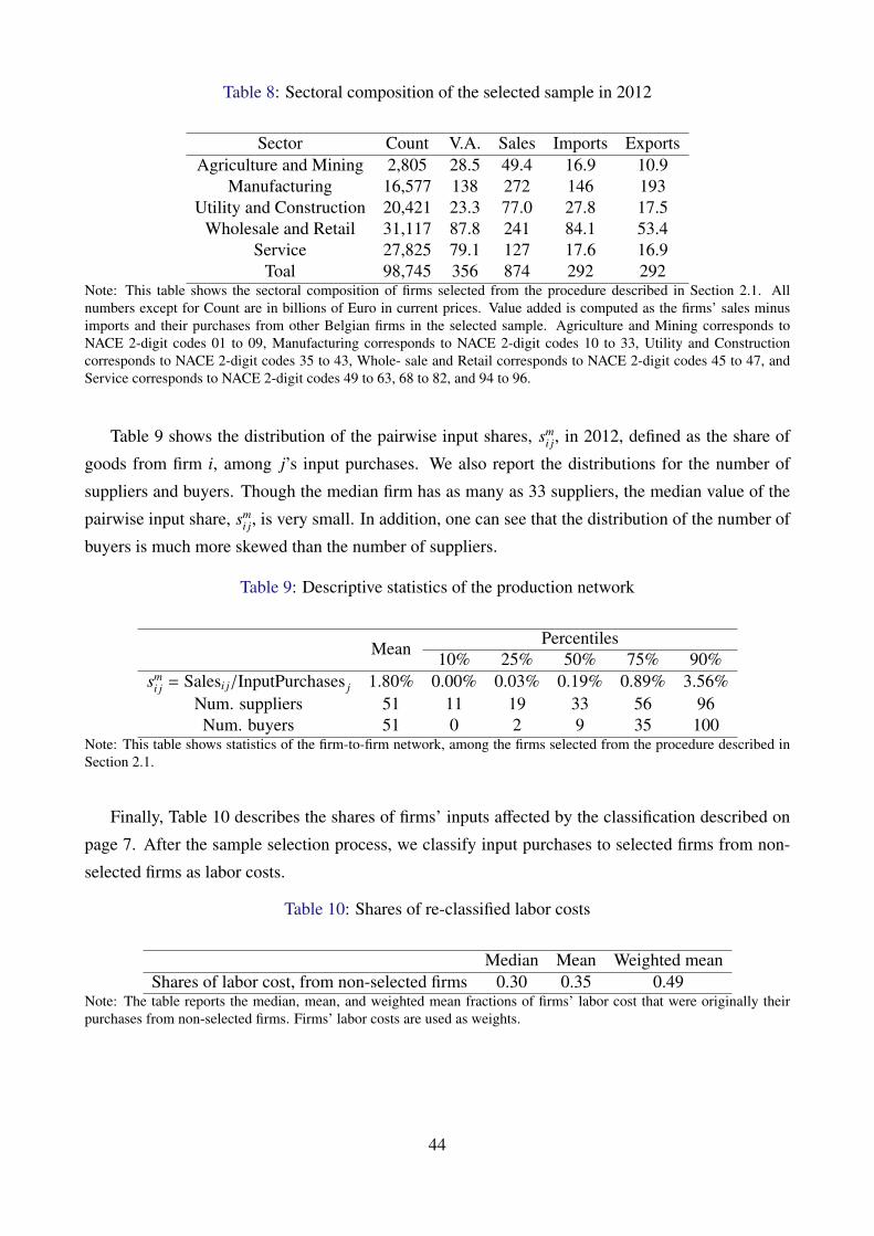
Table 8: Sectoral composition of the selected sample in 2012
Sector Count V.A. Sales Imports ExportsAgriculture and Mining 2,805 28.5 49.4 16.9 10.9
Manufacturing 16,577 138 272 146 193Utility and Construction 20,421 23.3 77.0 27.8 17.5
Wholesale and Retail 31,117 87.8 241 84.1 53.4Service 27,825 79.1 127 17.6 16.9
Toal 98,745 356 874 292 292Note: This table shows the sectoral composition of firms selected from the procedure described in Section 2.1. Allnumbers except for Count are in billions of Euro in current prices. Value added is computed as the firms’ sales minusimports and their purchases from other Belgian firms in the selected sample. Agriculture and Mining corresponds toNACE 2-digit codes 01 to 09, Manufacturing corresponds to NACE 2-digit codes 10 to 33, Utility and Constructioncorresponds to NACE 2-digit codes 35 to 43, Whole- sale and Retail corresponds to NACE 2-digit codes 45 to 47, andService corresponds to NACE 2-digit codes 49 to 63, 68 to 82, and 94 to 96.
Table 9 shows the distribution of the pairwise input shares, smi j, in 2012, defined as the share of
goods from firm i, among j’s input purchases. We also report the distributions for the number of
suppliers and buyers. Though the median firm has as many as 33 suppliers, the median value of the
pairwise input share, smi j, is very small. In addition, one can see that the distribution of the number of
buyers is much more skewed than the number of suppliers.
Table 9: Descriptive statistics of the production network
MeanPercentiles
10% 25% 50% 75% 90%sm
i j = Salesi j/InputPurchases j 1.80% 0.00% 0.03% 0.19% 0.89% 3.56%Num. suppliers 51 11 19 33 56 96Num. buyers 51 0 2 9 35 100
Note: This table shows statistics of the firm-to-firm network, among the firms selected from the procedure described inSection 2.1.
Finally, Table 10 describes the shares of firms’ inputs affected by the classification described on
page 7. After the sample selection process, we classify input purchases to selected firms from non-
selected firms as labor costs.
Table 10: Shares of re-classified labor costs
Median Mean Weighted meanShares of labor cost, from non-selected firms 0.30 0.35 0.49
Note: The table reports the median, mean, and weighted mean fractions of firms’ labor cost that were originally theirpurchases from non-selected firms. Firms’ labor costs are used as weights.
44
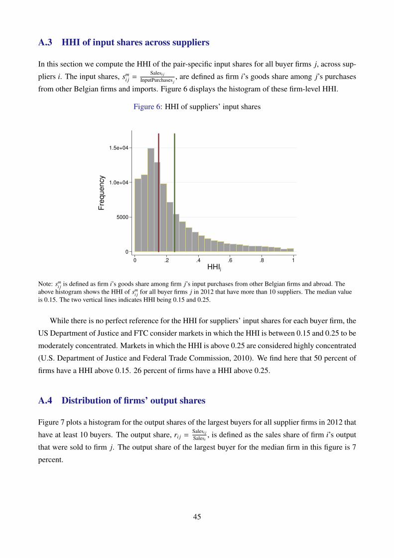
A.3 HHI of input shares across suppliers
In this section we compute the HHI of the pair-specific input shares for all buyer firms j, across sup-
pliers i. The input shares, smi j =
Salesi j
InputPurchases j, are defined as firm i’s goods share among j’s purchases
from other Belgian firms and imports. Figure 6 displays the histogram of these firm-level HHI.
Figure 6: HHI of suppliers’ input shares
0
5000
1.0e+04
1.5e+04
Fre
qu
en
cy
0 .2 .4 .6 .8 1
HHIj
Note: smi j is defined as firm i’s goods share among firm j’s input purchases from other Belgian firms and abroad. The
above histogram shows the HHI of smi j for all buyer firms j in 2012 that have more than 10 suppliers. The median value
is 0.15. The two vertical lines indicates HHI being 0.15 and 0.25.
While there is no perfect reference for the HHI for suppliers’ input shares for each buyer firm, the
US Department of Justice and FTC consider markets in which the HHI is between 0.15 and 0.25 to be
moderately concentrated. Markets in which the HHI is above 0.25 are considered highly concentrated
(U.S. Department of Justice and Federal Trade Commission, 2010). We find here that 50 percent of
firms have a HHI above 0.15. 26 percent of firms have a HHI above 0.25.
A.4 Distribution of firms’ output shares
Figure 7 plots a histogram for the output shares of the largest buyers for all supplier firms in 2012 that
have at least 10 buyers. The output share, ri j =Salesi j
Salesi, is defined as the sales share of firm i’s output
that were sold to firm j. The output share of the largest buyer for the median firm in this figure is 7
percent.
45
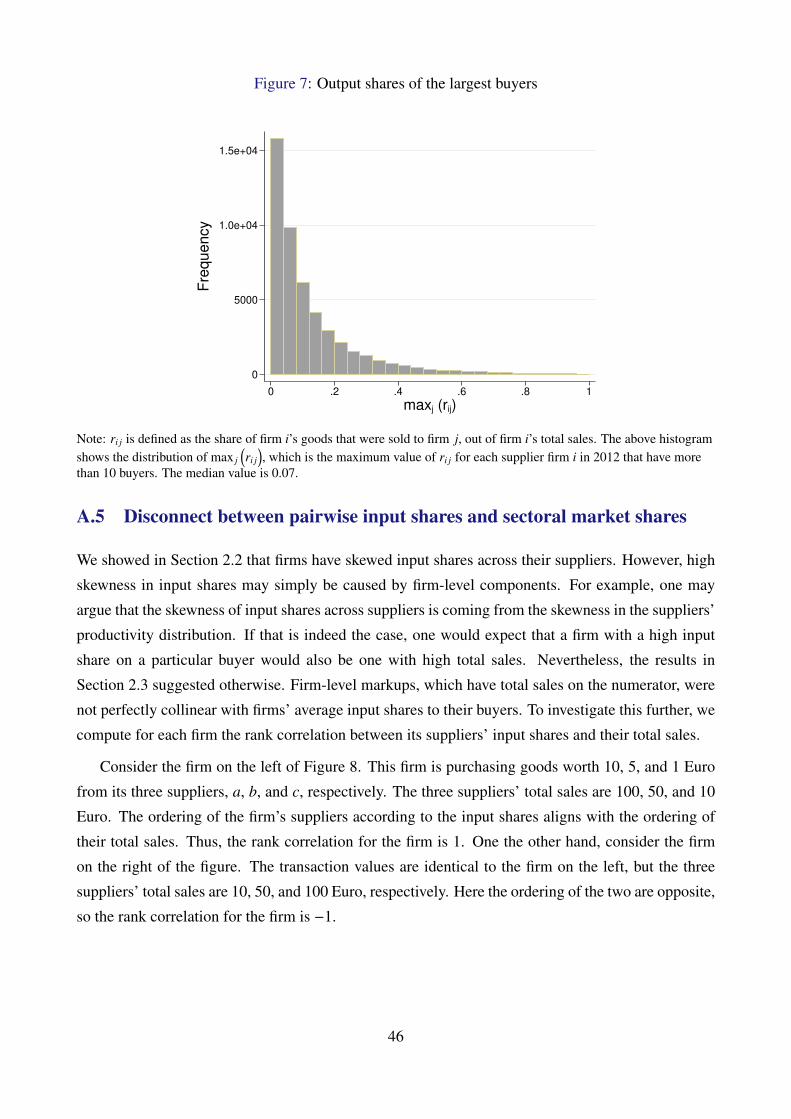
Figure 7: Output shares of the largest buyers
0
5000
1.0e+04
1.5e+04
Fre
qu
en
cy
0 .2 .4 .6 .8 1
maxj (rij)
Note: ri j is defined as the share of firm i’s goods that were sold to firm j, out of firm i’s total sales. The above histogramshows the distribution of max j
(ri j
), which is the maximum value of ri j for each supplier firm i in 2012 that have more
than 10 buyers. The median value is 0.07.
A.5 Disconnect between pairwise input shares and sectoral market shares
We showed in Section 2.2 that firms have skewed input shares across their suppliers. However, high
skewness in input shares may simply be caused by firm-level components. For example, one may
argue that the skewness of input shares across suppliers is coming from the skewness in the suppliers’
productivity distribution. If that is indeed the case, one would expect that a firm with a high input
share on a particular buyer would also be one with high total sales. Nevertheless, the results in
Section 2.3 suggested otherwise. Firm-level markups, which have total sales on the numerator, were
not perfectly collinear with firms’ average input shares to their buyers. To investigate this further, we
compute for each firm the rank correlation between its suppliers’ input shares and their total sales.
Consider the firm on the left of Figure 8. This firm is purchasing goods worth 10, 5, and 1 Euro
from its three suppliers, a, b, and c, respectively. The three suppliers’ total sales are 100, 50, and 10
Euro. The ordering of the firm’s suppliers according to the input shares aligns with the ordering of
their total sales. Thus, the rank correlation for the firm is 1. One the other hand, consider the firm
on the right of the figure. The transaction values are identical to the firm on the left, but the three
suppliers’ total sales are 10, 50, and 100 Euro, respectively. Here the ordering of the two are opposite,
so the rank correlation for the firm is −1.
46
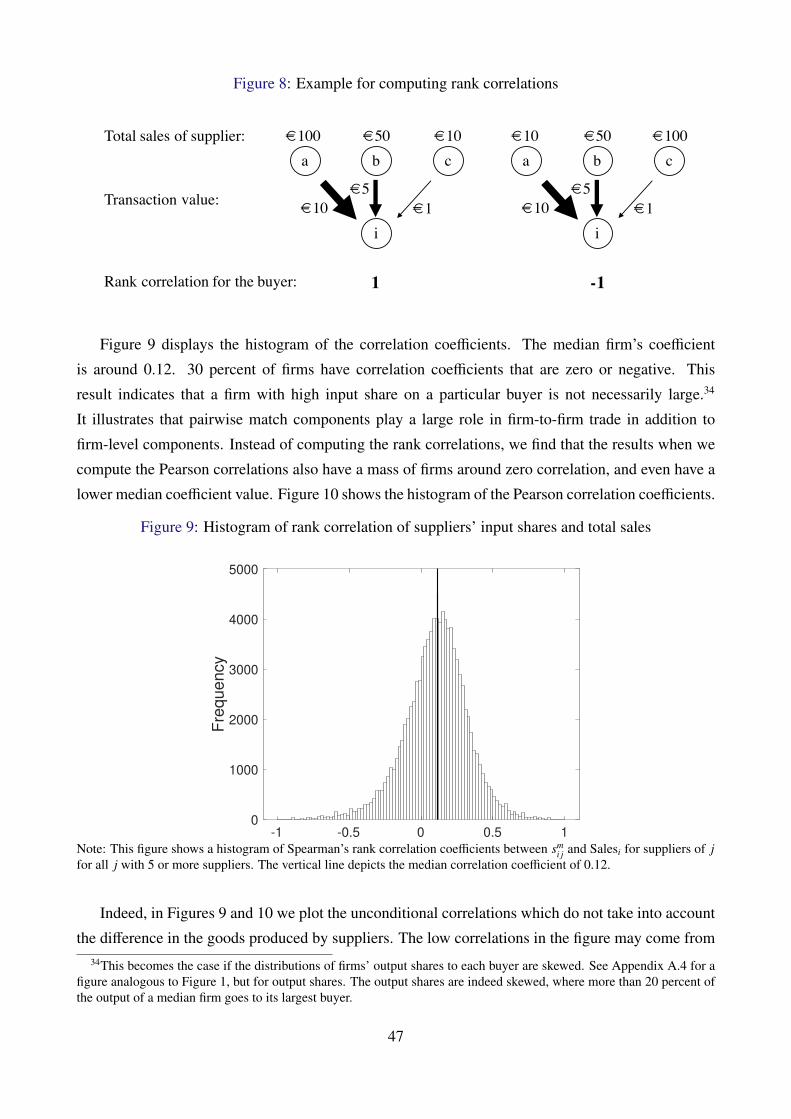
Figure 8: Example for computing rank correlations
i
ca bTotal sales of supplier: €100 €50 €10
Transaction value: €10€5
€1
1
i
ca b€10 €50 €100
€10€5
€1
-1Rank correlation for the buyer:
Figure 9 displays the histogram of the correlation coefficients. The median firm’s coefficient
is around 0.12. 30 percent of firms have correlation coefficients that are zero or negative. This
result indicates that a firm with high input share on a particular buyer is not necessarily large.34
It illustrates that pairwise match components play a large role in firm-to-firm trade in addition to
firm-level components. Instead of computing the rank correlations, we find that the results when we
compute the Pearson correlations also have a mass of firms around zero correlation, and even have a
lower median coefficient value. Figure 10 shows the histogram of the Pearson correlation coefficients.
Figure 9: Histogram of rank correlation of suppliers’ input shares and total sales
-1 -0.5 0 0.5 10
1000
2000
3000
4000
5000
Fre
quency
Note: This figure shows a histogram of Spearman’s rank correlation coefficients between smi j and Salesi for suppliers of j
for all j with 5 or more suppliers. The vertical line depicts the median correlation coefficient of 0.12.
Indeed, in Figures 9 and 10 we plot the unconditional correlations which do not take into account
the difference in the goods produced by suppliers. The low correlations in the figure may come from34This becomes the case if the distributions of firms’ output shares to each buyer are skewed. See Appendix A.4 for a
figure analogous to Figure 1, but for output shares. The output shares are indeed skewed, where more than 20 percent ofthe output of a median firm goes to its largest buyer.
47
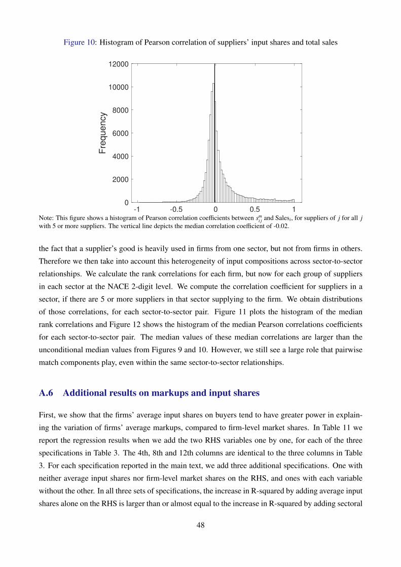
Figure 10: Histogram of Pearson correlation of suppliers’ input shares and total sales
-1 -0.5 0 0.5 10
2000
4000
6000
8000
10000
12000
Fre
qu
en
cy
Note: This figure shows a histogram of Pearson correlation coefficients between smi j and Salesi, for suppliers of j for all j
with 5 or more suppliers. The vertical line depicts the median correlation coefficient of -0.02.
the fact that a supplier’s good is heavily used in firms from one sector, but not from firms in others.
Therefore we then take into account this heterogeneity of input compositions across sector-to-sector
relationships. We calculate the rank correlations for each firm, but now for each group of suppliers
in each sector at the NACE 2-digit level. We compute the correlation coefficient for suppliers in a
sector, if there are 5 or more suppliers in that sector supplying to the firm. We obtain distributions
of those correlations, for each sector-to-sector pair. Figure 11 plots the histogram of the median
rank correlations and Figure 12 shows the histogram of the median Pearson correlations coefficients
for each sector-to-sector pair. The median values of these median correlations are larger than the
unconditional median values from Figures 9 and 10. However, we still see a large role that pairwise
match components play, even within the same sector-to-sector relationships.
A.6 Additional results on markups and input shares
First, we show that the firms’ average input shares on buyers tend to have greater power in explain-
ing the variation of firms’ average markups, compared to firm-level market shares. In Table 11 we
report the regression results when we add the two RHS variables one by one, for each of the three
specifications in Table 3. The 4th, 8th and 12th columns are identical to the three columns in Table
3. For each specification reported in the main text, we add three additional specifications. One with
neither average input shares nor firm-level market shares on the RHS, and ones with each variable
without the other. In all three sets of specifications, the increase in R-squared by adding average input
shares alone on the RHS is larger than or almost equal to the increase in R-squared by adding sectoral
48
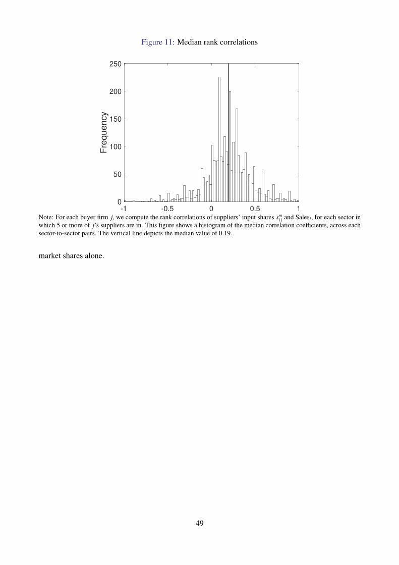
Figure 11: Median rank correlations
-1 -0.5 0 0.5 10
50
100
150
200
250
Fre
qu
en
cy
Note: For each buyer firm j, we compute the rank correlations of suppliers’ input shares smi j and Salesi, for each sector in
which 5 or more of j’s suppliers are in. This figure shows a histogram of the median correlation coefficients, across eachsector-to-sector pairs. The vertical line depicts the median value of 0.19.
market shares alone.
49
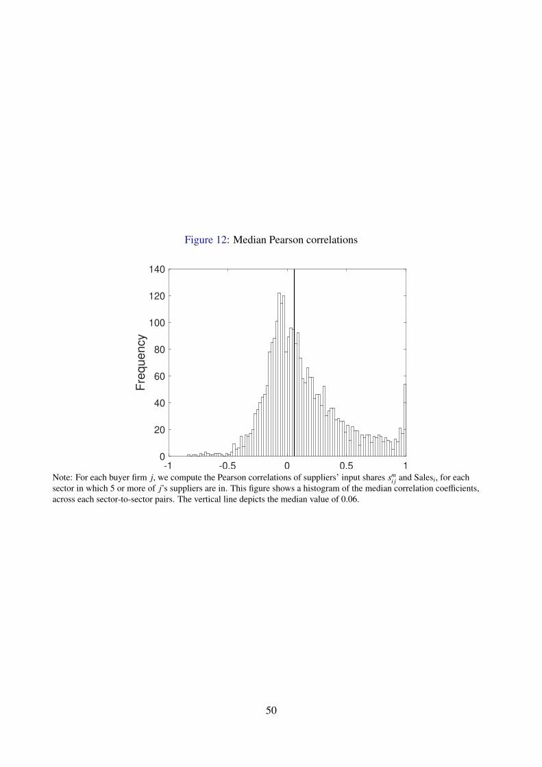
Figure 12: Median Pearson correlations
-1 -0.5 0 0.5 10
20
40
60
80
100
120
140
Fre
qu
en
cy
Note: For each buyer firm j, we compute the Pearson correlations of suppliers’ input shares smi j and Salesi, for each
sector in which 5 or more of j’s suppliers are in. This figure shows a histogram of the median correlation coefficients,across each sector-to-sector pairs. The vertical line depicts the median value of 0.06.
50

Tabl
e11
:Fir
m-l
evel
mar
kups
and
inpu
tsha
res,
R-s
quar
edac
ross
spec
ifica
tions
(1)
(2)
(3)
(4)
(5)
(6)
(7)
(8)
(9)
(10)
(11)
(12)
Sctr
Mkt
Shar
e i,t
(4-d
igit)
0.02
240.
0219
0.01
530.
0154
0.02
210.
0221
(0.0
0283
)(0
.002
80)
(0.0
0174
)(0
.001
74)
(0.0
0202
)(0
.002
01)
Ave
rage
inpu
tsha
resm i·,
t0.
0534
0.05
240.
0412
0.04
120.
0391
0.03
91(0
.003
96)
(0.0
0395
)(0
.002
99)
(0.0
0300
)(0
.002
91)
(0.0
0290
)N
8097
2280
9722
8097
2280
9722
7816
2778
1627
7816
2778
1627
7816
2778
1627
7816
2778
1627
Yea
rFE
Yes
Yes
Yes
Yes
Yes
Yes
Yes
Yes
Yes
Yes
Yes
Yes
Sect
orFE
4-di
git
4-di
git
4-di
git
4-di
git
No
No
No
No
No
No
No
No
Firm
FEN
oN
oN
oN
oY
esY
esY
esY
esY
esY
esY
esY
esC
ontr
ols
Yes
Yes
Yes
Yes
No
No
No
No
Yes
Yes
Yes
Yes
R2
0.10
330.
1040
0.10
430.
1050
0.63
750.
6376
0.63
770.
6378
0.63
850.
6387
0.63
870.
6389
Not
e:St
anda
rder
rors
inpa
rent
hese
s.T
heco
effici
ents
are
X-s
tand
ardi
zed.
Stan
dard
erro
rsar
ecl
uste
red
atth
eN
AC
E2-
digi
t-ye
arle
vel.
The
regr
essi
onex
clud
eou
tlier
sin
the
top
and
botto
m1
perc
ento
fthe
mar
kup
dist
ribu
tion.
Con
trol
sin
clud
efir
ms’
num
bero
fsup
plie
rs,n
umbe
rofb
uyer
s,em
ploy
men
t,to
tala
sset
s,an
dag
e.
51
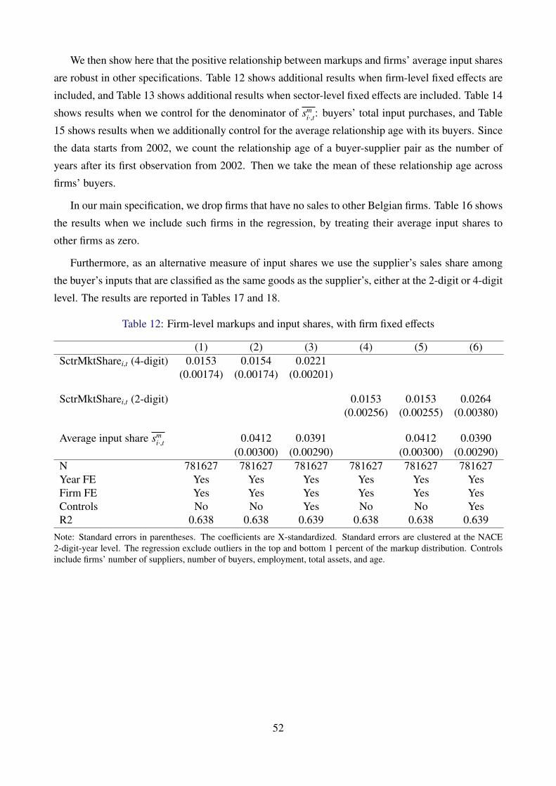
We then show here that the positive relationship between markups and firms’ average input shares
are robust in other specifications. Table 12 shows additional results when firm-level fixed effects are
included, and Table 13 shows additional results when sector-level fixed effects are included. Table 14
shows results when we control for the denominator of smi·,t: buyers’ total input purchases, and Table
15 shows results when we additionally control for the average relationship age with its buyers. Since
the data starts from 2002, we count the relationship age of a buyer-supplier pair as the number of
years after its first observation from 2002. Then we take the mean of these relationship age across
firms’ buyers.
In our main specification, we drop firms that have no sales to other Belgian firms. Table 16 shows
the results when we include such firms in the regression, by treating their average input shares to
other firms as zero.
Furthermore, as an alternative measure of input shares we use the supplier’s sales share among
the buyer’s inputs that are classified as the same goods as the supplier’s, either at the 2-digit or 4-digit
level. The results are reported in Tables 17 and 18.
Table 12: Firm-level markups and input shares, with firm fixed effects
(1) (2) (3) (4) (5) (6)SctrMktSharei,t (4-digit) 0.0153 0.0154 0.0221
(0.00174) (0.00174) (0.00201)
SctrMktSharei,t (2-digit) 0.0153 0.0153 0.0264(0.00256) (0.00255) (0.00380)
Average input share smi·,t 0.0412 0.0391 0.0412 0.0390
(0.00300) (0.00290) (0.00300) (0.00290)N 781627 781627 781627 781627 781627 781627Year FE Yes Yes Yes Yes Yes YesFirm FE Yes Yes Yes Yes Yes YesControls No No Yes No No YesR2 0.638 0.638 0.639 0.638 0.638 0.639
Note: Standard errors in parentheses. The coefficients are X-standardized. Standard errors are clustered at the NACE2-digit-year level. The regression exclude outliers in the top and bottom 1 percent of the markup distribution. Controlsinclude firms’ number of suppliers, number of buyers, employment, total assets, and age.
52

Table 13: Firm-level markups and input shares, with sector fixed effects
(1) (2) (3) (4)SctrMktSharei,t (4-digit) 0.0224 0.0219
(0.00283) (0.00280)
SctrMktSharei,t (2-digit) 0.0220 0.0215(0.00226) (0.00223)
Average input share smi·,t 0.0524 0.0540
(0.00395) (0.00422)N 809722 809722 809727 809727Year FE Yes Yes Yes YesSector FE 4-digit 4-digit 2-digit 2-digitControls Yes Yes Yes YesR2 0.104 0.105 0.0719 0.0729
Note: Standard errors in parentheses. The coefficients are X-standardized. Standard errors are clustered at the NACE2-digit-year level. The regression exclude outliers in the top and bottom 1 percent of the markup distribution. Controlsinclude firms’ number of suppliers, number of buyers, employment, total assets, and age.
Table 14: Firm-level markups and input shares, controlling for buyers’ size
(1) (2)SctrMktSharei,t (4-digit) 0.0235 0.0221
(0.00264) (0.00201)
Average input share smi·,t 0.0417 0.0385
(0.00358) (0.00291)N 809722 781627Year FE Yes YesSector FE 4-digit NoFirm FE No YesControls Yes YesR2 0.108 0.639
Note: Standard errors in parentheses. The coefficients are X-standardized. Standard errors are clustered at the NACE2-digit-year level. The regression exclude outliers in the top and bottom 1 percent of the markup distribution. Controlsinclude firms’ number of suppliers, number of buyers, employment, total assets, age, and buyers’ total input purchases.
53
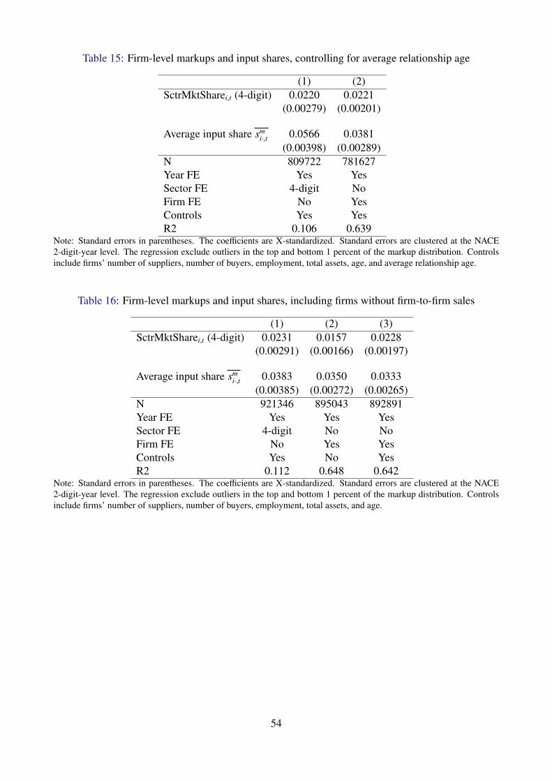
Table 15: Firm-level markups and input shares, controlling for average relationship age
(1) (2)SctrMktSharei,t (4-digit) 0.0220 0.0221
(0.00279) (0.00201)
Average input share smi·,t 0.0566 0.0381
(0.00398) (0.00289)N 809722 781627Year FE Yes YesSector FE 4-digit NoFirm FE No YesControls Yes YesR2 0.106 0.639
Note: Standard errors in parentheses. The coefficients are X-standardized. Standard errors are clustered at the NACE2-digit-year level. The regression exclude outliers in the top and bottom 1 percent of the markup distribution. Controlsinclude firms’ number of suppliers, number of buyers, employment, total assets, age, and average relationship age.
Table 16: Firm-level markups and input shares, including firms without firm-to-firm sales
(1) (2) (3)SctrMktSharei,t (4-digit) 0.0231 0.0157 0.0228
(0.00291) (0.00166) (0.00197)
Average input share smi·,t 0.0383 0.0350 0.0333
(0.00385) (0.00272) (0.00265)N 921346 895043 892891Year FE Yes Yes YesSector FE 4-digit No NoFirm FE No Yes YesControls Yes No YesR2 0.112 0.648 0.642
Note: Standard errors in parentheses. The coefficients are X-standardized. Standard errors are clustered at the NACE2-digit-year level. The regression exclude outliers in the top and bottom 1 percent of the markup distribution. Controlsinclude firms’ number of suppliers, number of buyers, employment, total assets, and age.
54
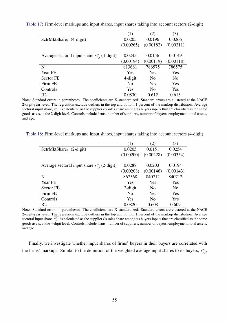
Table 17: Firm-level markups and input shares, input shares taking into account sectors (2-digit)
(1) (2) (3)SctrMktSharei,t (4-digit) 0.0205 0.0196 0.0266
(0.00265) (0.00182) (0.00211)
Average sectoral input share smi·,t (4-digit) 0.0245 0.0156 0.0149
(0.00194) (0.00119) (0.00118)N 813681 786575 786575Year FE Yes Yes YesSector FE 4-digit No NoFirm FE No Yes YesControls Yes No YesR2 0.0830 0.612 0.613
Note: Standard errors in parentheses. The coefficients are X-standardized. Standard errors are clustered at the NACE2-digit-year level. The regression exclude outliers in the top and bottom 1 percent of the markup distribution. Averagesectoral input share, sm
i·,t, is calculated as the supplier i’s sales share among its buyers inputs that are classified as the samegoods as i’s, at the 2-digit level. Controls include firms’ number of suppliers, number of buyers, employment, total assets,and age.
Table 18: Firm-level markups and input shares, input shares taking into account sectors (4-digit)
(1) (2) (3)SctrMktSharei,t (2-digit) 0.0205 0.0151 0.0254
(0.00200) (0.00228) (0.00354)
Average sectoral input share smi·,t (2-digit) 0.0288 0.0203 0.0194
(0.00208) (0.00146) (0.00143)N 867568 840712 840712Year FE Yes Yes YesSector FE 2-digit No NoFirm FE No Yes YesControls Yes No YesR2 0.0820 0.608 0.609
Note: Standard errors in parentheses. The coefficients are X-standardized. Standard errors are clustered at the NACE2-digit-year level. The regression exclude outliers in the top and bottom 1 percent of the markup distribution. Averagesectoral input share, sm
i·,t, is calculated as the supplier i’s sales share among its buyers inputs that are classified as the samegoods as i’s, at the 4-digit level. Controls include firms’ number of suppliers, number of buyers, employment, total assets,and age.
Finally, we investigate whether input shares of firms’ buyers in their buyers are correlated with
the firms’ markups. Similar to the definition of the weighted average input shares to its buyers, smi·,t,
55
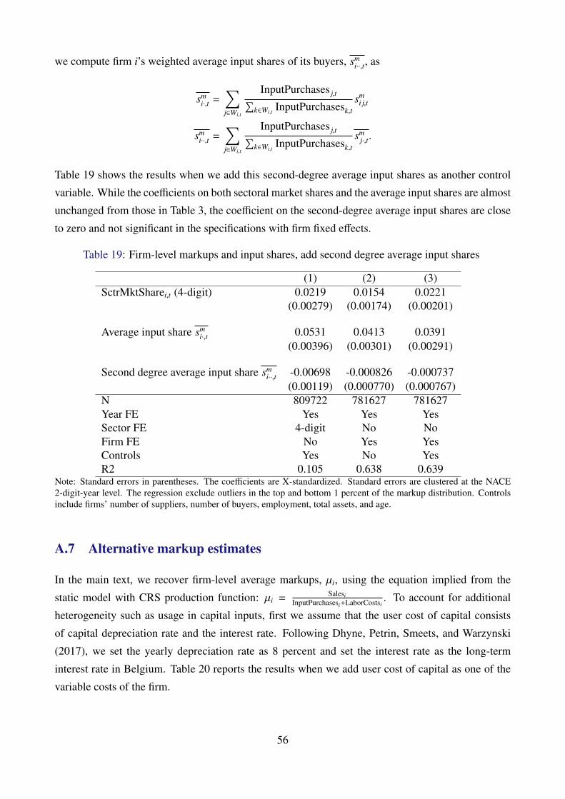
we compute firm i’s weighted average input shares of its buyers, smi··,t, as
smi·,t =
∑j∈Wi,t
InputPurchases j,t∑k∈Wi,t
InputPurchasesk,tsm
i j,t
smi··,t =
∑j∈Wi,t
InputPurchases j,t∑k∈Wi,t
InputPurchasesk,tsm
j·,t.
Table 19 shows the results when we add this second-degree average input shares as another control
variable. While the coefficients on both sectoral market shares and the average input shares are almost
unchanged from those in Table 3, the coefficient on the second-degree average input shares are close
to zero and not significant in the specifications with firm fixed effects.
Table 19: Firm-level markups and input shares, add second degree average input shares
(1) (2) (3)SctrMktSharei,t (4-digit) 0.0219 0.0154 0.0221
(0.00279) (0.00174) (0.00201)
Average input share smi·,t 0.0531 0.0413 0.0391
(0.00396) (0.00301) (0.00291)
Second degree average input share smi··,t -0.00698 -0.000826 -0.000737
(0.00119) (0.000770) (0.000767)N 809722 781627 781627Year FE Yes Yes YesSector FE 4-digit No NoFirm FE No Yes YesControls Yes No YesR2 0.105 0.638 0.639
Note: Standard errors in parentheses. The coefficients are X-standardized. Standard errors are clustered at the NACE2-digit-year level. The regression exclude outliers in the top and bottom 1 percent of the markup distribution. Controlsinclude firms’ number of suppliers, number of buyers, employment, total assets, and age.
A.7 Alternative markup estimates
In the main text, we recover firm-level average markups, µi, using the equation implied from the
static model with CRS production function: µi = SalesiInputPurchasesi+LaborCostsi
. To account for additional
heterogeneity such as usage in capital inputs, first we assume that the user cost of capital consists
of capital depreciation rate and the interest rate. Following Dhyne, Petrin, Smeets, and Warzynski
(2017), we set the yearly depreciation rate as 8 percent and set the interest rate as the long-term
interest rate in Belgium. Table 20 reports the results when we add user cost of capital as one of the
variable costs of the firm.
56
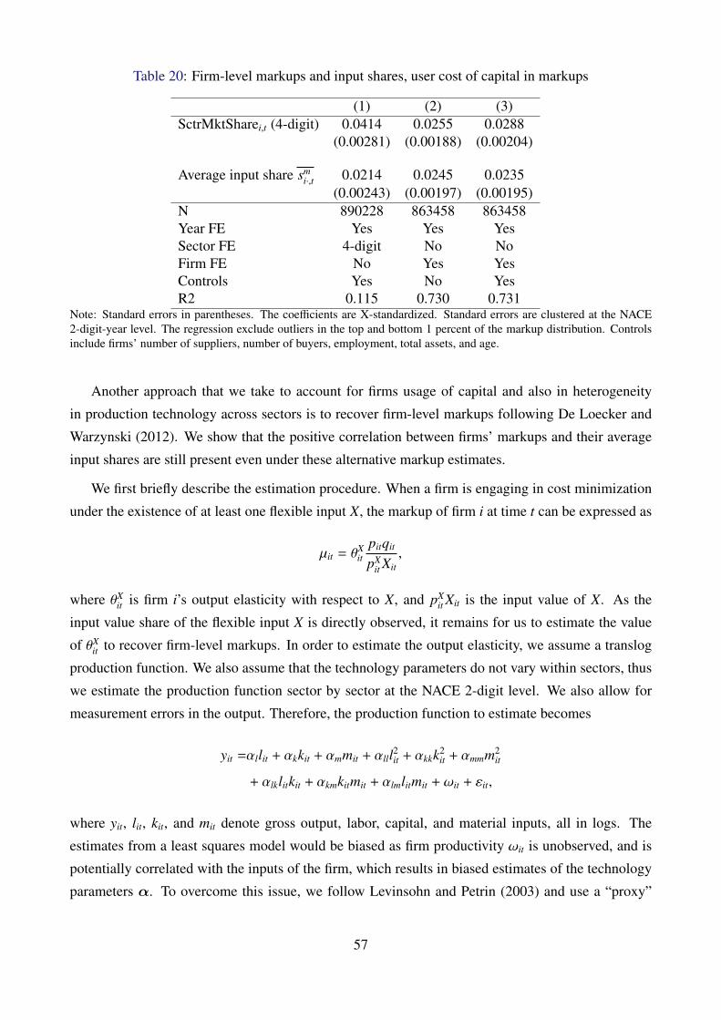
Table 20: Firm-level markups and input shares, user cost of capital in markups
(1) (2) (3)SctrMktSharei,t (4-digit) 0.0414 0.0255 0.0288
(0.00281) (0.00188) (0.00204)
Average input share smi·,t 0.0214 0.0245 0.0235
(0.00243) (0.00197) (0.00195)N 890228 863458 863458Year FE Yes Yes YesSector FE 4-digit No NoFirm FE No Yes YesControls Yes No YesR2 0.115 0.730 0.731
Note: Standard errors in parentheses. The coefficients are X-standardized. Standard errors are clustered at the NACE2-digit-year level. The regression exclude outliers in the top and bottom 1 percent of the markup distribution. Controlsinclude firms’ number of suppliers, number of buyers, employment, total assets, and age.
Another approach that we take to account for firms usage of capital and also in heterogeneity
in production technology across sectors is to recover firm-level markups following De Loecker and
Warzynski (2012). We show that the positive correlation between firms’ markups and their average
input shares are still present even under these alternative markup estimates.
We first briefly describe the estimation procedure. When a firm is engaging in cost minimization
under the existence of at least one flexible input X, the markup of firm i at time t can be expressed as
µit = θXit
pitqit
pXit Xit
,
where θXit is firm i’s output elasticity with respect to X, and pX
it Xit is the input value of X. As the
input value share of the flexible input X is directly observed, it remains for us to estimate the value
of θXit to recover firm-level markups. In order to estimate the output elasticity, we assume a translog
production function. We also assume that the technology parameters do not vary within sectors, thus
we estimate the production function sector by sector at the NACE 2-digit level. We also allow for
measurement errors in the output. Therefore, the production function to estimate becomes
yit =αllit + αkkit + αmmit + αlll2it + αkkk2
it + αmmm2it
+ αlklitkit + αkmkitmit + αlmlitmit + ωit + εit,
where yit, lit, kit, and mit denote gross output, labor, capital, and material inputs, all in logs. The
estimates from a least squares model would be biased as firm productivity ωit is unobserved, and is
potentially correlated with the inputs of the firm, which results in biased estimates of the technology
parameters α. To overcome this issue, we follow Levinsohn and Petrin (2003) and use a “proxy”
57
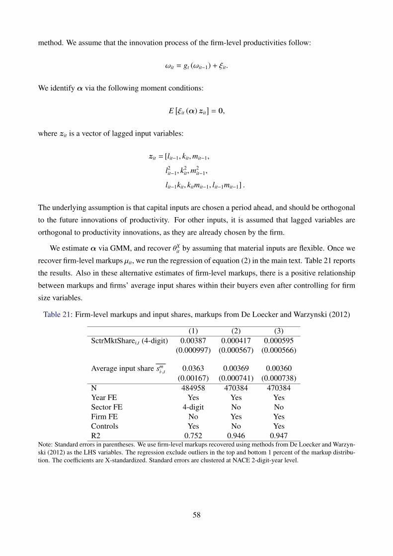
method. We assume that the innovation process of the firm-level productivities follow:
ωit = gt (ωit−1) + ξit.
We identify α via the following moment conditions:
E[ξit (α) zit
]= 0,
where zit is a vector of lagged input variables:
zit = [lit−1, kit,mit−1,
l2it−1, k
2it,m
2it−1,
lit−1kit, kitmit−1, lit−1mit−1] .
The underlying assumption is that capital inputs are chosen a period ahead, and should be orthogonal
to the future innovations of productivity. For other inputs, it is assumed that lagged variables are
orthogonal to productivity innovations, as they are already chosen by the firm.
We estimate α via GMM, and recover θXit by assuming that material inputs are flexible. Once we
recover firm-level markups µit, we run the regression of equation (2) in the main text. Table 21 reports
the results. Also in these alternative estimates of firm-level markups, there is a positive relationship
between markups and firms’ average input shares within their buyers even after controlling for firm
size variables.
Table 21: Firm-level markups and input shares, markups from De Loecker and Warzynski (2012)
(1) (2) (3)SctrMktSharei,t (4-digit) 0.00387 0.000417 0.000595
(0.000997) (0.000567) (0.000566)
Average input share smi·,t 0.0363 0.00369 0.00360
(0.00167) (0.000741) (0.000738)N 484958 470384 470384Year FE Yes Yes YesSector FE 4-digit No NoFirm FE No Yes YesControls Yes No YesR2 0.752 0.946 0.947
Note: Standard errors in parentheses. We use firm-level markups recovered using methods from De Loecker and Warzyn-ski (2012) as the LHS variables. The regression exclude outliers in the top and bottom 1 percent of the markup distribu-tion. The coefficients are X-standardized. Standard errors are clustered at NACE 2-digit-year level.
58

B Theoretical results
B.1 Derivation of equation (14)
Consider firm j selling its goods to i. Firm j chooses p ji to maximize profits, taking into account the
effect of p ji on i’s price indices for its intermediate goods, pmi and pmv( j)i. It takes as given i’s unit cost
and production, ci, and qi, as well as i’s sourcing sets, Zi and IFi. The firm’s problem is as follows:
maxp ji
(p ji − c j
)q ji
s.t.q ji = ασv( j)
ji αρ
v( j) p−σv( j)
ji
(pm
v( j)i
)σv( j)−1 (pm
v( j)i
)1−ρpρmimi
mi = ωηm p−ηmiφ
η−1i cηi qi.
Solving the above problem while taking into account that ∂pmi∂p ji, 0 and
∂pmv( j)i
∂p ji, 0 yields
p ji =ε ji
ε ji − 1c j
ε ji = σv( j)
(1 − sv( j)
ji
)+ ρsv( j)
ji
(1 − sm
v( j)i
)+ ηsv( j)
ji smv( j)i.
B.2 Alternative market structures
In our model we assume the following when firms participate in firm-to-firm trade. When selling to
firm i, firm j sets price p ji by internalizing the effect of p ji on j’s price indices for its intermediate
goods, pmi and pmv( j)i. However, it takes as given i’s unit cost and total production, ci and qi. This
yields our pricing equation of
p ji =ε ji
ε ji − 1c j
ε ji = σv( j)
(1 − sv( j)
ji
)+ ρsv( j)
ji
(1 − sm
v( j)i
)+ ηsv( j)
ji smv( j)i.
In this section we discuss alternative market structures in firm-to-firm trade.
B.2.1 Cournot competition
Instead of assuming Bertrand competition one can alternatively assume that firms engage in Cournot
competition, where firms set quantity q ji to maximize variable profits. In that case, the demand
elasticity that firm j faces, ε ji, becomes a weighted harmonic mean of the CES parameters σv( j), ρ,
59
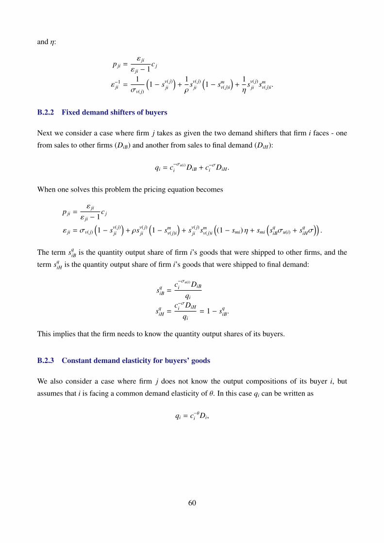
and η:
p ji =ε ji
ε ji − 1c j
ε−1ji =
1σv( j)
(1 − sv( j)
ji
)+
1ρ
sv( j)ji
(1 − sm
v( j)i
)+
1η
sv( j)ji sm
v( j)i.
B.2.2 Fixed demand shifters of buyers
Next we consider a case where firm j takes as given the two demand shifters that firm i faces - one
from sales to other firms (DiB) and another from sales to final demand (DiH):
qi = c−σu(i)i DiB + c−σi DiH.
When one solves this problem the pricing equation becomes
p ji =ε ji
ε ji − 1c j
ε ji = σv( j)
(1 − sv( j)
ji
)+ ρsv( j)
ji
(1 − sm
v( j)i
)+ sv( j)
ji smv( j)i
((1 − smi) η + smi
(sq
iBσu(i) + sqiHσ
)).
The term sqiB is the quantity output share of firm i’s goods that were shipped to other firms, and the
term sqiH is the quantity output share of firm i’s goods that were shipped to final demand:
sqiB =
c−σu(i)i DiB
qi
sqiH =
c−σi DiH
qi= 1 − sq
iB.
This implies that the firm needs to know the quantity output shares of its buyers.
B.2.3 Constant demand elasticity for buyers’ goods
We also consider a case where firm j does not know the output compositions of its buyer i, but
assumes that i is facing a common demand elasticity of θ. In this case qi can be written as
qi = c−θi Di,
60

in which firm j takes as given the demand shifter, Di. When one solves the problem of firm j under
this setup, the pricing equation becomes
p ji =ε ji
ε ji − 1c j
ε ji = σv( j)
(1 − sv( j)
ji
)+ ρsv( j)
ji
(1 − sm
v( j)i
)+ sv( j)
ji smv( j)i ((1 − smi) η + smiθ) .
Notice that if we additionally assume that θ = η, the above equation collapses to equation (14).
B.3 System of equilibrium changes upon changes in markups
B.3.1 System of exact changes
In this section we take the observed firm-to-firm trade network, and present the system of equations
that pins down changes in the equilibrium variables upon exogenous changes inµi j
.
The total variable inputs observed in the data is denoted by ciqi = wli +∑
k Vki + VFi. Also denote
total input cost of firm i implied from the model as Ci =∑
jVi j
µi j+ ViH
µiH+ ViF
µiH. The difference between
the two is denoted as ξi = ciqi − Ci. We take the error term in equation (21), εi =ξi
ciqi, as constants.
With this assumption, the changes in the observed inputs, ciqi∧
, are equal to the changes in the model
implied inputs, Ci, and also to the changes in the difference between the two, ξi. We also denote trade
balance as T B and treat them as fixed.
We now have the following system of equations defining the equilibrium:
E = wL +∑
i
πi −∑
i
ξi − T B
πi =∑k∈Wi
µik − 1µik
Vik +µiH − 1µiH
(ViH + ViF)
Vik = su(i)ik sm
u(i)ksmkckqk
ViH = siHE
ViF = µ1−σiH c1−σ
i D∗
ξi = ciqi −Ci
= ciqi −
ViH
µiH+
ViF
µiH+
∑j
Vi j
µi j
.From this system, we then proceed with the following steps and compute the hat-variables upon µi j.
1. Guess the change in nominal wage, w.
61

2. Compute the changes in prices with
c1−ηi = sliw1−η + smi p
1−ηmi
p1−ρmi =
∑v
smvi(pm
vi)1−ρ
+ smFi(
pmvi)1−σv =
∑j∈Zi, j∈V
sv( j)ji µ
1−σvji c1−σv( j)
j .
3. Compute other variables’ changes with
sv( j)ji = µ
1−σv( j)
ji c1−σv( j)
j
(pm
v( j)i
)σv( j)−1
smvi =
(pm
vi)1−ρ pρ−1
mi
smi = p1−ηmi cη−1
i
sli = w1−ηcη−1i
s ji = sv( j)ji sm
v( j)i smi
P =
∑i
siH c1−σi
1
1−σ
siH = c1−σi Pσ−1
ViF = c1−σi .
4. Compute Ci from
Ci =1Ci
ViH
µiHsiH E +
1Ci
ViF
µiHViF +
1Ci
∑j
Vi j si j
µi jµi jC j
E =1
1 −∑
i1EµiH−1µiH
ViH siH
×
wLE
w −T BE−
∑i ξiCi
E+
∑i
πi
E
∑k
1πi
Vikµikµik − 1µikµik
sikCk +1πi
µiH − 1µiH
ViFViF
.
5. Update w from
w =1
wL
∑i
sliciqi sliCi,
and iterate from Step 1 until w converges.
B.3.2 System of first-order approximated changes
We take the system of equilibrium changes in the previous section and solve for the first-order ap-
proximated changes. Now we denote the shock withdµi j
µi j
.
62
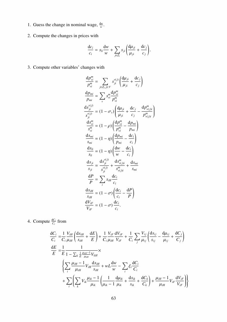
1. Guess the change in nominal wage, dww .
2. Compute the changes in prices with
dci
ci= sli
dww
+∑j∈Zi
s ji
(dµ ji
µ ji+
dc j
c j
).
3. Compute other variables’ changes with
dpmvi
pmvi
=∑
j∈Zi, j∈V
sv( j)ji
(dµ ji
µ ji+
dc j
c j
)dpmi
pmi=
∑v
smvi
dpmvi
pmvi
dsv( j)ji
sv( j)ji
= (1 − σv)
dµ ji
µ ji+
dc j
c j−
dpmv( j)i
pmv( j)i
dsm
vi
smvi
= (1 − ρ)(dpm
vi
pmvi−
dpmi
pmi
)dsmi
smi= (1 − η)
(dpmi
pmi−
dci
ci
)dsli
sli= (1 − η)
(dww−
dci
ci
)ds ji
s ji=
dsv( j)ji
sv( j)ji
+dsm
v( j)i
smv( j)i
+dsmi
smi
dPP
=∑
i
siHdci
ci
dsiH
siH= (1 − σ)
(dci
ci−
dPP
)dViF
ViF= (1 − σ)
dci
ci.
4. Compute dCiCi
from
dCi
Ci=
1Ci
ViH
µiH
(dsiH
siH+
dEE
)+
1Ci
ViF
µiH
dViF
ViF+
1Ci
∑j
Vi j
µi j
(dsi j
si j−
dµi j
µi j+
dC j
C j
)dEE
=1E
1
1 −∑
k1EµkH−1µkH
VkH
×∑i
µiH − 1µiH
ViHdsiH
siH+ wL
dww−
∑i
ξidCi
Ci
+∑
i
∑k
Vikµik − 1µik
(1
µik − 1dµik
µik+
dsik
sik+
dCk
Ck
)+µiH − 1µiH
ViFdViF
ViF
63

5. Update dww from
dww
=1
wL
∑i
wli
(dsli
sli+
dCi
Ci
),
and iterate from Step 1 until dww converges.
B.4 System of equilibrium changes upon changes in markups, sectoralroundabout production network
We also consider a sectoral roundabout production network that is consistent with the observed firm-
level data, and present the system of equations that pins down changes in the equilibrium variables
upon exogenous changes in markups. We consider a network where there two distinct composite
goods, one of which is used as intermediate goods and another of which is used as a final consumption
good. The cost function for firm i is expressed by equation (20). As in the previous section, the total
variable inputs observed in the data is denoted by ciqi = wli +∑
k Vki + VFi, and the total input cost
of firm i implied from the model is denoted as Ci =∑
jVi j
µiB+ ViH
µiH+ ViF
µiH. The difference between the
two is denoted as ξi = ciqi − Ci. We also assume that the error terms in the estimating equation (22),
εi =ξi
ciqi, are constants. Therefore we have ξi = ciqi
∧= Ci.
We assume that firms charge constant markups µi =∑
j Vi j+ViH+ViF
Cito both composite goods. This as-
sumption makes markups at the firm-level consistent with the baseline model with variable markups.
We take the reduction in the markups that firms charge to the composite good used for intermediate
inputs, µiBR , as the shock.
Before proceeding with the following steps, we first compute the share of sector u goods in house-
hold consumption as γuH =∑
i∈u ViH∑i ViH
. Denote the share of sector v goods in the domestic intermediate
input bundle for sector u as γvu =∑
i∈v∑
j∈u Vi j∑k∑
j∈u Vk j. Also denote sH
iu(i) as firm i’s share of sales to household
among other firms in the same sector, thus siH = sHiu(i)γu(i)H. Analogously, denote sB
iu(i) as firm i’s share
of sales to other firms, among other firms in the same sector.
1. Guess the change in nominal wage, w.
2. Compute the changes in prices with
c1−ηi = sliw1−η + smi p
1−ηmi
p1−ρmi = sm
Di
∏v
Pγvu(i)vB
1−ρ
+ smFi
P1−σv( j)
v( j)B =∑j∈V
sBjv( j)µ
1−σv( j)
jBRc1−σv( j)
j .
64

3. Compute other variables’ changes with
P1−σvH =
∑j∈v
sHjv( j)c
1−σj
P =∏
v
PγvHvH
smDi =
∏v
Pγvu(i)vB
1−ρ
pρ−1mi
smi = p1−ηmi cη−1
i
sli = w1−ηcη−1i
sBiu(i) = µ
1−σu(i)iBR
c1−σu(i)i Pσu(i)−1
u(i)B
sHiu(i) = c1−σ
i Pσ−1u(i)H
ViF = c1−σi .
4. Compute Ci from
Ci =1Ci
siHEµi
sHiu(i)E +
1Ci
sBiu(i) s
Biu(i)
µiµiBR
∑v
γu(i)v
∑j∈v
VD j smD j sm jC j
+1Ci
ViF
µiViF
E =1
1 −∑
iµi−1µi
siH sHiu(i)
×
wLE
w +1E
∑i
µiµiBR − 1µiµiBR
sBiu(i) s
Biu(i)
∑v
γu(i)v
∑j∈v
VD j smD j sm jC j
+
1E
∑i
µi − 1µi
ViFViF −T BE−
∑i ξiCi
E
5. Update w from
w =1
wL
∑i
wli sliCi,
and iterate from Step 1 until w converges.
B.5 System of equilibrium changes upon changes in the foreign price
Here we present the system of equations that pins down changes in the equilibrium variables upon an
exogenous change in the price of foreign goods, pF .
65

B.5.1 System of exact changes
First we present the system under endogenous markups. Unlike the system in Appendix B.3, markupsµi j
are endogenous variables. In this section, we assume that the error terms in the estimating
equation (22), εi =ξi
ciqi, are constants. Therefore we have ξi = ciqi
∧= Ci.
We first focus on the exact changes, and follow the steps below.
1. Guess the change in nominal wage, w.
2. Compute the changes in prices and shares with
c1−ηi = sliw1−η + smi p
1−ηmi
p1−ρmi =
∑v
smvi(pm
vi)1−ρ
+ smFi p
1−ρF(
pmvi)1−σv =
∑j∈Zi, j∈V
sv( j)ji µ
1−σvji c1−σv
j
µ ji = ε jiε ji − 1ε jiε ji − 1
ε ji = σv( j)
(1 − sv( j)
ji
)+ ρsv( j)
ji
(1 − sm
v( j)i
)+ ηsv( j)
ji smv( j)i
ε ji =1ε ji
(σv( j)
(1 − sv( j)
ji sv( j)ji
)+ ρsv( j)
ji sv( j)ji
(1 − sm
v( j)i smv( j)i
)+ ηsv( j)
ji smv( j)i s
v( j)ji sm
v( j)i
)sv( j)
ji = µ1−σv( j)
ji c1−σv( j)
j
(pm
v( j)i
)σv( j)−1
smvi =
(pm
vi)1−ρ pρ−1
mi .
3. Compute other changes in prices and shares with
smi = p1−ηmi cη−1
i
sli = w1−ηcη−1i
s ji = sv( j)ji sm
v( j)i smi
P =
∑i
siH c1−σi
1
1−σ
siH = c1−σi Pσ−1
ViF = c1−σi .
66

4. Compute Ci from
Ci =1Ci
ViH
µiHsiH E +
1Ci
ViF
µiHViF +
1Ci
∑j
Vi j si j
µi jµi jC j
E =1
1 −∑
i1EµiH−1µiH
ViH siH
×
wLE
w −∑
i
ξi
ECi −
T BE
+∑
i
πi
E
∑k
1πi
Vikµikµik − 1µikµik
sikCk +1πi
µiH − 1µiH
ViFViF
.
5. Update w from
w =1
wL
∑i
sliciqi sliCi,
and iterate from Step 1 until w converges.
B.5.2 System of first-order approximated changes
We then turn to the system of first-order approximated changes. Taking first order approximations of
the system presented in the previous section, we obtain the following steps.
1. Guess the change in nominal wage, dww .
2. Compute the changes in prices and markups with
dci
ci=sli
dww
+∑j∈Zi
s ji
(dµ ji
µ ji+
dc j
c j
)+ sFi
dpF
pF
dµ ji
µ ji= − Γ ji
dc j
c j+ Γ ji
dp6 jip6 ji
,
where Γ ji equals the elasticity of markup µ ji with respect to the supplier’s cost c j:
Γ ji = −∂µ ji
∂c j
c j
µ ji
=Υ ji
1 + Υ ji
Υ ji =
(ε ji − σv( j)
) (1 − σv( j)
) (1 − sv( j)
ji
)+ sv( j)
ji (η − ρ) (1 − ρ) sv( j)ji
(1 − sm
v( j)i
)sm
v( j)i
ε ji
(ε ji − 1
) .
The term dp6 jip6 ji
is expressed as:
dp6 jip6 ji
=Υ·∈V ( j)·i
Υ ji
∑k∈V ( j),k, j
sv( j)ki
(dµki
µki+
dck
ck
)+
ΥU (·),v( j)·i
Υ ji
∑k∈U ,u,v( j)
smki
(dµki
µki+
dck
ck
)+ sm
FidpF
pF
67

where
Υ·∈V ( j)·i =
(ε ji − σv( j)
) (1 − σv( j)
)− (η − ρ) (1 − ρ) sv( j)
ji
(1 − sm
v( j)i
)sm
v( j)i
ε ji
(ε ji − 1
)Υ
U (·),v( j)·i =
sv( j)ji (η − ρ) (1 − ρ) sm
v( j)i
ε ji
(ε ji − 1
) .
dp6 jip6 ji
is the weighted average of the price changes of i’s suppliers other than j, with suppliers in
the same sector as j’s sector (k ∈ V ( j) , k , j) and suppliers in different sectors as j’s sector
(k ∈ U , u , v ( j)) having different elasticity weights.35
3. Compute other changes in prices and shares with
dpmvi
pmvi
=∑
j∈Zi, j∈V
sv( j)ji
(dµ ji
µ ji+
dc j
c j
)dpmi
pmi=
∑v
smvi
dpmvi
pmvi
+ smFi
dpF
pF
dsv( j)ji
sv( j)ji
= (1 − σv)(dµ ji
µ ji+
dc j
c j−
dpmvi
pmvi
)dsm
vi
smvi
= (1 − ρ)(dpm
vi
pmvi−
dpmi
pmi
)dsmi
smi= (1 − η)
(dpmi
pmi−
dci
ci
)dsli
sli= (1 − η)
(dww−
dci
ci
)ds ji
s ji=
dsv( j)ji
sv( j)ji
+dsm
v( j)i
smv( j)i
+dsmi
smi
dPP
=∑
i
siHdci
ci
dsiH
siH= (1 − σ)
(dci
ci−
dPP
)dViF
ViF= (1 − σ)
dci
ci.
35For illustration, consider a single-sector model where we impose σu = ρ. Then we obtain Υ ji =(ε ji−ρ)(1−ρ)
(1−sm
ji
)ε ji(ε ji−1) and
dp6 jip6 ji
= 11−sm
ji
(∑k, j sm
ki
(dµkiµki
+ dckck
)+ sm
FidpFpF
).
68

4. Compute dCiCi
from
dCi
Ci=
1Ci
ViH
µiH
(dsiH
siH+
dEE
)+
1Ci
ViF
µiH
dViF
ViF+
1Ci
∑j
Vi j
µi j
(dsi j
si j−
dµi j
µi j+
dC j
C j
)dEE
=1E
1
1 −∑
k1EµkH−1µkH
VkH
×∑i
µiH − 1µiH
ViHdsiH
siH+ wL
dww−
∑i
ξidCi
Ci
+∑
i
∑k
Vikµik − 1µik
(1
µik − 1dµik
µik+
dsik
sik+
dCk
Ck
)+µiH − 1µiH
ViFdViF
ViF
5. Update dww from
dww
=1
wL
∑i
wli
(dsli
sli+
dCi
Ci
).
B.6 System of equilibrium changes upon changes in the foreign price,constant markups
Now we consider the system under constant markups, where firms charge heterogeneous markups of
µi j and µiH as in the baseline economy. We back-out these markups as we do for the baseline economy,
but treat them as fixed in the counterfactual exercise. As in the previous section, we assume that the
error terms in the estimating equation (22), εi =ξi
ciqi, are constants.
1. Guess the change in nominal wage, w.
2. Compute the changes in prices and shares with
c1−ηi = sliw1−η + smi p
1−ηmi
p1−ρmi =
∑v
smvi(pm
vi)1−ρ
+ smFi p
1−ρF(
pmvi)1−σv =
∑j∈Zi, j∈V
sv( j)ji c1−σv
j .
69
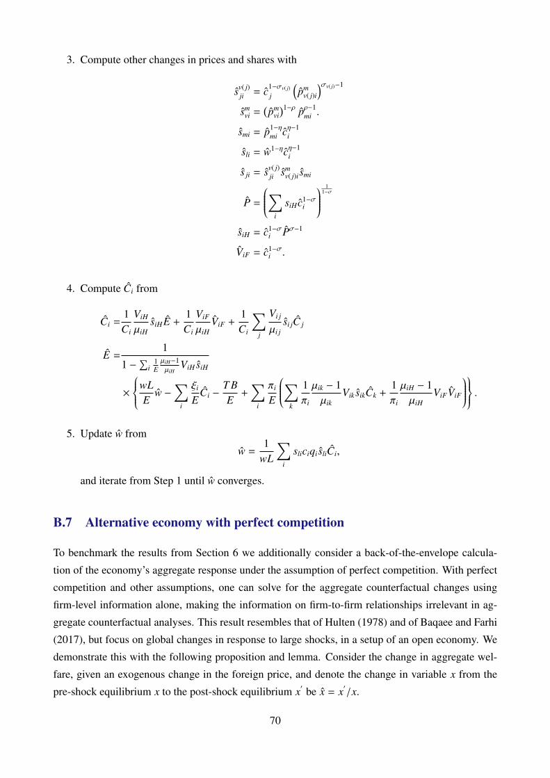
3. Compute other changes in prices and shares with
sv( j)ji = c1−σv( j)
j
(pm
v( j)i
)σv( j)−1
smvi =
(pm
vi)1−ρ pρ−1
mi .
smi = p1−ηmi cη−1
i
sli = w1−ηcη−1i
s ji = sv( j)ji sm
v( j)i smi
P =
∑i
siH c1−σi
1
1−σ
siH = c1−σi Pσ−1
ViF = c1−σi .
4. Compute Ci from
Ci =1Ci
ViH
µiHsiH E +
1Ci
ViF
µiHViF +
1Ci
∑j
Vi j
µi jsi jC j
E =1
1 −∑
i1EµiH−1µiH
ViH siH
×
wLE
w −∑
i
ξi
ECi −
T BE
+∑
i
πi
E
∑k
1πi
µik − 1µik
Vik sikCk +1πi
µiH − 1µiH
ViFViF
.
5. Update w from
w =1
wL
∑i
sliciqi sliCi,
and iterate from Step 1 until w converges.
B.7 Alternative economy with perfect competition
To benchmark the results from Section 6 we additionally consider a back-of-the-envelope calcula-
tion of the economy’s aggregate response under the assumption of perfect competition. With perfect
competition and other assumptions, one can solve for the aggregate counterfactual changes using
firm-level information alone, making the information on firm-to-firm relationships irrelevant in ag-
gregate counterfactual analyses. This result resembles that of Hulten (1978) and of Baqaee and Farhi
(2017), but focus on global changes in response to large shocks, in a setup of an open economy. We
demonstrate this with the following proposition and lemma. Consider the change in aggregate wel-
fare, given an exogenous change in the foreign price, and denote the change in variable x from the
pre-shock equilibrium x to the post-shock equilibrium x′
be x = x′
/x.
70
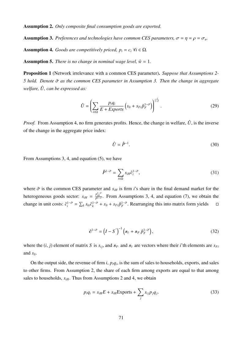
Assumption 2. Only composite final consumption goods are exported.
Assumption 3. Preferences and technologies have common CES parameters, σ = η = ρ = σu.
Assumption 4. Goods are competitively priced, pi = ci ∀i ∈ Ω.
Assumption 5. There is no change in nominal wage level, w = 1.
Proposition 1 (Network irrelevance with a common CES parameter). Suppose that Assumptions 2-
5 hold. Denote σ as the common CES parameter in Assumption 3. Then the change in aggregate
welfare, U, can be expressed as:
U =
∑i∈Ω
piqi
E + Exports
(sli + sFi p1−σ
F
)−1
1−σ
. (29)
Proof. From Assumption 4, no firm generates profits. Hence, the change in welfare, U, is the inverse
of the change in the aggregate price index:
U = P−1. (30)
From Assumptions 3, 4, and equation (5), we have
P1−σ =∑i∈Ω
siH c1−σi , (31)
where σ is the common CES parameter and siH is firm i’s share in the final demand market for the
heterogeneous goods sector: siH =p1−σ
iHP1−σ . From Assumptions 3, 4, and equation (7), we obtain the
change in unit costs: c1−σi =
∑k skic1−σ
k + sli + sFi p1−σF . Rearranging this into matrix form yields
c1−σ =(I − S
′)−1 (
sl· + sF· p1−σF
), (32)
where the (i, j) element of matrix S is si j, and sF· and sl· are vectors where their i’th elements are sFi
and sli.
On the output side, the revenue of firm i, piqi, is the sum of sales to households, exports, and sales
to other firms. From Assumption 2, the share of each firm among exports are equal to that among
sales to households, siH. Thus from Assumptions 2 and 4, we obtain
piqi = siHE + siHExports +∑
j
si j p jq j. (33)
71
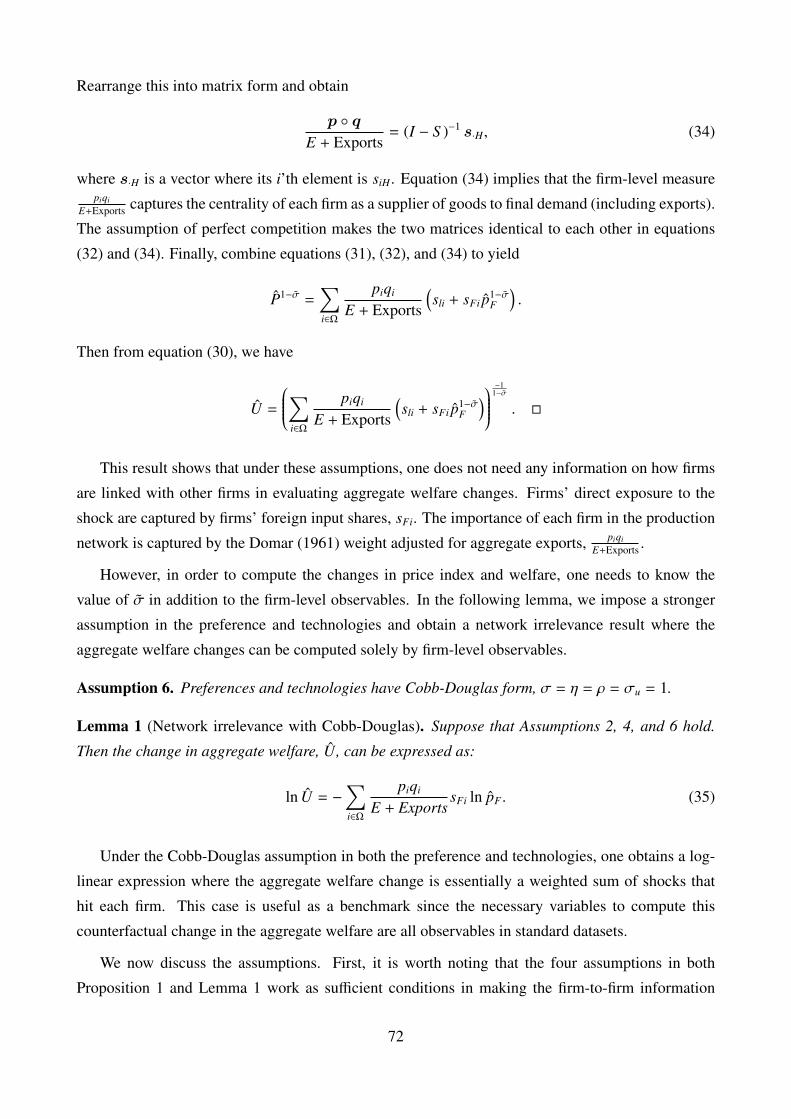
Rearrange this into matrix form and obtain
p q
E + Exports= (I − S )−1 s·H, (34)
where s·H is a vector where its i’th element is siH. Equation (34) implies that the firm-level measurepiqi
E+Exports captures the centrality of each firm as a supplier of goods to final demand (including exports).
The assumption of perfect competition makes the two matrices identical to each other in equations
(32) and (34). Finally, combine equations (31), (32), and (34) to yield
P1−σ =∑i∈Ω
piqi
E + Exports
(sli + sFi p1−σ
F
).
Then from equation (30), we have
U =
∑i∈Ω
piqi
E + Exports
(sli + sFi p1−σ
F
)−1
1−σ
.
This result shows that under these assumptions, one does not need any information on how firms
are linked with other firms in evaluating aggregate welfare changes. Firms’ direct exposure to the
shock are captured by firms’ foreign input shares, sFi. The importance of each firm in the production
network is captured by the Domar (1961) weight adjusted for aggregate exports, piqiE+Exports .
However, in order to compute the changes in price index and welfare, one needs to know the
value of σ in addition to the firm-level observables. In the following lemma, we impose a stronger
assumption in the preference and technologies and obtain a network irrelevance result where the
aggregate welfare changes can be computed solely by firm-level observables.
Assumption 6. Preferences and technologies have Cobb-Douglas form, σ = η = ρ = σu = 1.
Lemma 1 (Network irrelevance with Cobb-Douglas). Suppose that Assumptions 2, 4, and 6 hold.
Then the change in aggregate welfare, U, can be expressed as:
ln U = −∑i∈Ω
piqi
E + ExportssFi ln pF . (35)
Under the Cobb-Douglas assumption in both the preference and technologies, one obtains a log-
linear expression where the aggregate welfare change is essentially a weighted sum of shocks that
hit each firm. This case is useful as a benchmark since the necessary variables to compute this
counterfactual change in the aggregate welfare are all observables in standard datasets.
We now discuss the assumptions. First, it is worth noting that the four assumptions in both
Proposition 1 and Lemma 1 work as sufficient conditions in making the firm-to-firm information
72
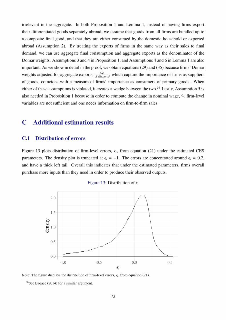
irrelevant in the aggregate. In both Proposition 1 and Lemma 1, instead of having firms export
their differentiated goods separately abroad, we assume that goods from all firms are bundled up to
a composite final good, and that they are either consumed by the domestic household or exported
abroad (Assumption 2). By treating the exports of firms in the same way as their sales to final
demand, we can use aggregate final consumption and aggregate exports as the denominator of the
Domar weights. Assumptions 3 and 4 in Proposition 1, and Assumptions 4 and 6 in Lemma 1 are also
important. As we show in detail in the proof, we obtain equations (29) and (35) because firms’ Domar
weights adjusted for aggregate exports, piqiE+Exports , which capture the importance of firms as suppliers
of goods, coincides with a measure of firms’ importance as consumers of primary goods. When
either of these assumptions is violated, it creates a wedge between the two.36 Lastly, Assumption 5 is
also needed in Proposition 1 because in order to compute the change in nominal wage, w, firm-level
variables are not sufficient and one needs information on firm-to-firm sales.
C Additional estimation results
C.1 Distribution of errors
Figure 13 plots distribution of firm-level errors, εi, from equation (21) under the estimated CES
parameters. The density plot is truncated at εi = −1. The errors are concentrated around εi = 0.2,
and have a thick left tail. Overall this indicates that under the estimated parameters, firms overall
purchase more inputs than they need in order to produce their observed outputs.
Figure 13: Distribution of εi
0.0
0.5
1.0
1.5
2.0
-1.0 -0.5 0.0 0.5εi
dens
ity
Note: The figure displays the distribution of firm-level errors, εi, from equation (21).
36See Baqaee (2014) for a similar argument.
73

C.2 Assuming Cournot competition
When assuming Cournot competition in firm-to-firm trade instead, equation (14) becomes
p ji =ε ji
ε ji − 1c j
ε ji =
(1
σv( j)
(1 − sv( j)
ji
)+
1ρ
sv( j)ji
(1 − sm
v( j)i
)+
1η
sv( j)ji sm
v( j)i
)−1
.
We follow the same procedure described in Section 4 and obtain the estimates shown in Table 22.
74
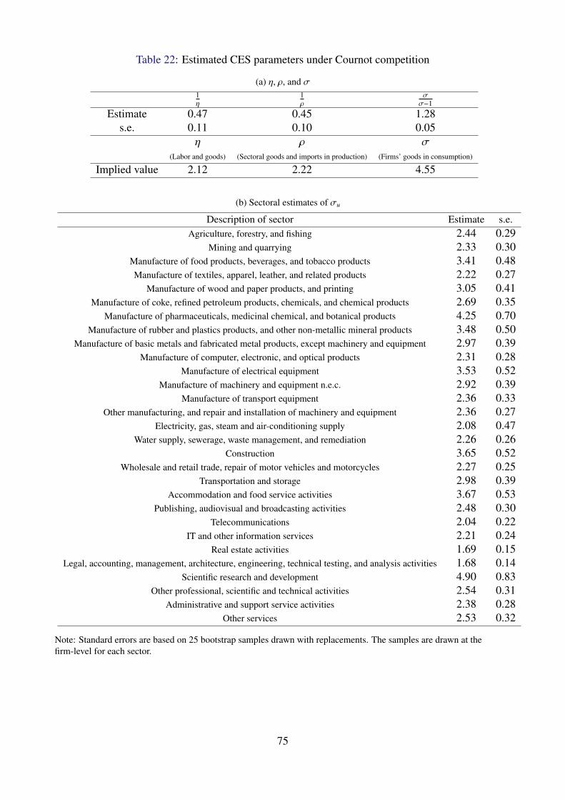
Table 22: Estimated CES parameters under Cournot competition
(a) η, ρ, and σ1η
1ρ
σσ−1
Estimate 0.47 0.45 1.28s.e. 0.11 0.10 0.05
η ρ σ(Labor and goods) (Sectoral goods and imports in production) (Firms’ goods in consumption)
Implied value 2.12 2.22 4.55
(b) Sectoral estimates of σu
Description of sector Estimate s.e.Agriculture, forestry, and fishing 2.44 0.29
Mining and quarrying 2.33 0.30Manufacture of food products, beverages, and tobacco products 3.41 0.48Manufacture of textiles, apparel, leather, and related products 2.22 0.27
Manufacture of wood and paper products, and printing 3.05 0.41Manufacture of coke, refined petroleum products, chemicals, and chemical products 2.69 0.35
Manufacture of pharmaceuticals, medicinal chemical, and botanical products 4.25 0.70Manufacture of rubber and plastics products, and other non-metallic mineral products 3.48 0.50
Manufacture of basic metals and fabricated metal products, except machinery and equipment 2.97 0.39Manufacture of computer, electronic, and optical products 2.31 0.28
Manufacture of electrical equipment 3.53 0.52Manufacture of machinery and equipment n.e.c. 2.92 0.39
Manufacture of transport equipment 2.36 0.33Other manufacturing, and repair and installation of machinery and equipment 2.36 0.27
Electricity, gas, steam and air-conditioning supply 2.08 0.47Water supply, sewerage, waste management, and remediation 2.26 0.26
Construction 3.65 0.52Wholesale and retail trade, repair of motor vehicles and motorcycles 2.27 0.25
Transportation and storage 2.98 0.39Accommodation and food service activities 3.67 0.53
Publishing, audiovisual and broadcasting activities 2.48 0.30Telecommunications 2.04 0.22
IT and other information services 2.21 0.24Real estate activities 1.69 0.15
Legal, accounting, management, architecture, engineering, technical testing, and analysis activities 1.68 0.14Scientific research and development 4.90 0.83
Other professional, scientific and technical activities 2.54 0.31Administrative and support service activities 2.38 0.28
Other services 2.53 0.32
Note: Standard errors are based on 25 bootstrap samples drawn with replacements. The samples are drawn at thefirm-level for each sector.
75

C.3 Accounting for capital inputs
In the model, total input ciqi is an aggregate of labor costs and goods purchases. Here we account for
capital inputs by interpreting labor as the composite input of labor and capital. As we do not directly
observe capital rental costs for each firm, we take two alternate approaches.
First, we assume that firms have common labor shares, and uniformly scale up labor cost. We
use the aggregate labor share of 2/3 that we compute as the total labor cost divided by the total value
added. Second, we assume that the user cost of capital consists of capital depreciation rate and the
interest rate. Following Dhyne, Petrin, Smeets, and Warzynski (2017), we set the yearly depreciation
rate as 8 percent and set the interest rate as the long-term interest rate in Belgium. We compute
the capital rental costs using fixed tangible assets reported in the annual accounts. We report the
estimation results in Table 23.
76
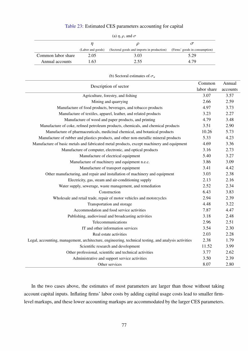
Table 23: Estimated CES parameters accounting for capital
(a) η, ρ, and σ
η ρ σ(Labor and goods) (Sectoral goods and imports in production) (Firms’ goods in consumption)
Common labor share 2.05 3.03 5.29Annual accounts 1.63 2.55 4.79
(b) Sectoral estimates of σu
Description of sectorCommon Annual
labor share accountsAgriculture, forestry, and fishing 3.07 3.57
Mining and quarrying 2.66 2.59Manufacture of food products, beverages, and tobacco products 4.97 3.73Manufacture of textiles, apparel, leather, and related products 3.23 2.27
Manufacture of wood and paper products, and printing 4.79 3.48Manufacture of coke, refined petroleum products, chemicals, and chemical products 3.51 2.90
Manufacture of pharmaceuticals, medicinal chemical, and botanical products 10.26 5.73Manufacture of rubber and plastics products, and other non-metallic mineral products 5.33 4.23
Manufacture of basic metals and fabricated metal products, except machinery and equipment 4.69 3.36Manufacture of computer, electronic, and optical products 3.16 2.73
Manufacture of electrical equipment 5.40 3.27Manufacture of machinery and equipment n.e.c. 3.86 3.09
Manufacture of transport equipment 3.41 4.42Other manufacturing, and repair and installation of machinery and equipment 3.03 2.38
Electricity, gas, steam and air-conditioning supply 2.13 2.16Water supply, sewerage, waste management, and remediation 2.52 2.34
Construction 6.43 3.83Wholesale and retail trade, repair of motor vehicles and motorcycles 2.94 2.39
Transportation and storage 4.48 3.22Accommodation and food service activities 7.87 4.47
Publishing, audiovisual and broadcasting activities 3.18 2.48Telecommunications 2.96 2.51
IT and other information services 3.54 2.30Real estate activities 2.03 2.28
Legal, accounting, management, architecture, engineering, technical testing, and analysis activities 2.38 1.79Scientific research and development 11.52 3.99
Other professional, scientific and technical activities 3.77 2.62Administrative and support service activities 3.50 2.39
Other services 8.07 2.80
In the two cases above, the estimates of most parameters are larger than those without taking
account capital inputs. Inflating firms’ labor costs by adding capital usage costs lead to smaller firm-
level markups, and these lower accounting markups are accommodated by the larger CES parameters.
77
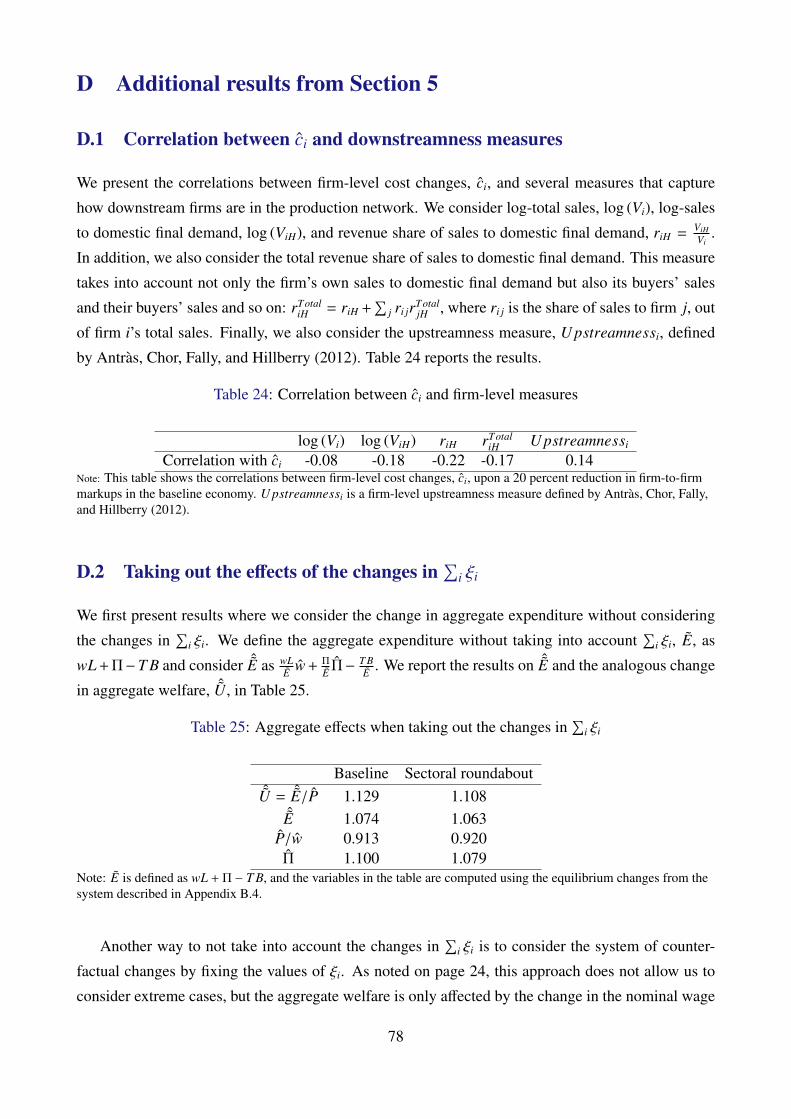
D Additional results from Section 5
D.1 Correlation between ci and downstreamness measures
We present the correlations between firm-level cost changes, ci, and several measures that capture
how downstream firms are in the production network. We consider log-total sales, log (Vi), log-sales
to domestic final demand, log (ViH), and revenue share of sales to domestic final demand, riH = ViHVi
.
In addition, we also consider the total revenue share of sales to domestic final demand. This measure
takes into account not only the firm’s own sales to domestic final demand but also its buyers’ sales
and their buyers’ sales and so on: rTotaliH = riH +
∑j ri jrTotal
jH , where ri j is the share of sales to firm j, out
of firm i’s total sales. Finally, we also consider the upstreamness measure, U pstreamnessi, defined
by Antras, Chor, Fally, and Hillberry (2012). Table 24 reports the results.
Table 24: Correlation between ci and firm-level measures
log (Vi) log (ViH) riH rTotaliH U pstreamnessi
Correlation with ci -0.08 -0.18 -0.22 -0.17 0.14Note: This table shows the correlations between firm-level cost changes, ci, upon a 20 percent reduction in firm-to-firmmarkups in the baseline economy. U pstreamnessi is a firm-level upstreamness measure defined by Antras, Chor, Fally,and Hillberry (2012).
D.2 Taking out the effects of the changes in∑
i ξi
We first present results where we consider the change in aggregate expenditure without considering
the changes in∑
i ξi. We define the aggregate expenditure without taking into account∑
i ξi, E, as
wL + Π−T B and consider ˆE as wLE w + Π
E Π− T BE . We report the results on ˆE and the analogous change
in aggregate welfare, ˆU, in Table 25.
Table 25: Aggregate effects when taking out the changes in∑
i ξi
Baseline Sectoral roundaboutˆU = ˆE/P 1.129 1.108
ˆE 1.074 1.063P/w 0.913 0.920Π 1.100 1.079
Note: E is defined as wL + Π − T B, and the variables in the table are computed using the equilibrium changes from thesystem described in Appendix B.4.
Another way to not take into account the changes in∑
i ξi is to consider the system of counter-
factual changes by fixing the values of ξi. As noted on page 24, this approach does not allow us to
consider extreme cases, but the aggregate welfare is only affected by the change in the nominal wage
78
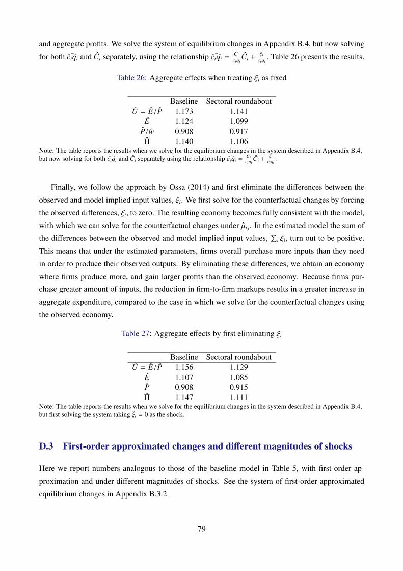
and aggregate profits. We solve the system of equilibrium changes in Appendix B.4, but now solving
for both ciqi∧
and Ci separately, using the relationship ciqi∧
= Ciciqi
Ci +ξi
ciqi. Table 26 presents the results.
Table 26: Aggregate effects when treating ξi as fixed
Baseline Sectoral roundaboutU = E/P 1.173 1.141
E 1.124 1.099P/w 0.908 0.917Π 1.140 1.106
Note: The table reports the results when we solve for the equilibrium changes in the system described in Appendix B.4,but now solving for both ciqi
∧and Ci separately using the relationship ciqi
∧= Ci
ciqiCi +
ξiciqi
.
Finally, we follow the approach by Ossa (2014) and first eliminate the differences between the
observed and model implied input values, ξi. We first solve for the counterfactual changes by forcing
the observed differences, ξi, to zero. The resulting economy becomes fully consistent with the model,
with which we can solve for the counterfactual changes under µi j. In the estimated model the sum of
the differences between the observed and model implied input values,∑
i ξi, turn out to be positive.
This means that under the estimated parameters, firms overall purchase more inputs than they need
in order to produce their observed outputs. By eliminating these differences, we obtain an economy
where firms produce more, and gain larger profits than the observed economy. Because firms pur-
chase greater amount of inputs, the reduction in firm-to-firm markups results in a greater increase in
aggregate expenditure, compared to the case in which we solve for the counterfactual changes using
the observed economy.
Table 27: Aggregate effects by first eliminating ξi
Baseline Sectoral roundaboutU = E/P 1.156 1.129
E 1.107 1.085P 0.908 0.915Π 1.147 1.111
Note: The table reports the results when we solve for the equilibrium changes in the system described in Appendix B.4,but first solving the system taking ξi = 0 as the shock.
D.3 First-order approximated changes and different magnitudes of shocks
Here we report numbers analogous to those of the baseline model in Table 5, with first-order ap-
proximation and under different magnitudes of shocks. See the system of first-order approximated
equilibrium changes in Appendix B.3.2.
79
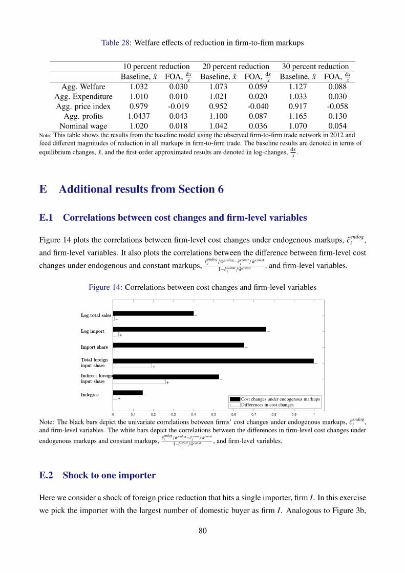
Table 28: Welfare effects of reduction in firm-to-firm markups
10 percent reduction 20 percent reduction 30 percent reductionBaseline, x FOA, dx
x Baseline, x FOA, dxx Baseline, x FOA, dx
xAgg. Welfare 1.032 0.030 1.073 0.059 1.127 0.088
Agg. Expenditure 1.010 0.010 1.021 0.020 1.033 0.030Agg. price index 0.979 -0.019 0.952 -0.040 0.917 -0.058
Agg. profits 1.0437 0.043 1.100 0.087 1.165 0.130Nominal wage 1.020 0.018 1.042 0.036 1.070 0.054
Note: This table shows the results from the baseline model using the observed firm-to-firm trade network in 2012 andfeed different magnitudes of reduction in all markups in firm-to-firm trade. The baseline results are denoted in terms ofequilibrium changes, x, and the first-order approximated results are denoted in log-changes, dx
x .
E Additional results from Section 6
E.1 Correlations between cost changes and firm-level variables
Figure 14 plots the correlations between firm-level cost changes under endogenous markups, cendogi ,
and firm-level variables. It also plots the correlations between the difference between firm-level cost
changes under endogenous and constant markups, cendogi /wendog−cconst
i /wconst
1−cconsti /wconst , and firm-level variables.
Figure 14: Correlations between cost changes and firm-level variables
+
+
+
+
0 0.1 0.2 0.3 0.4 0.5 0.6 0.7 0.8 0.9 1
Cost changes under endogenous markups
Differences in cost changes
Note: The black bars depict the univariate correlations between firms’ cost changes under endogenous markups, cendogi ,
and firm-level variables. The white bars depict the correlations between the differences in firm-level cost changes under
endogenous markups and constant markups, cendogi /wendog−cconst
i /wconst
1−cconsti /wconst , and firm-level variables.
E.2 Shock to one importer
Here we consider a shock of foreign price reduction that hits a single importer, firm I. In this exercise
we pick the importer with the largest number of domestic buyer as firm I. Analogous to Figure 3b,
80

we first plot the differences in firm-level cost changes normalized for changes in nominal wages,
across two economies: the baseline economy and the economy with constant markups. We plot
the histogram of these differences in Figure 15. Compared to Figure 3b in which we consider a
uniform foreign price change that affected all importers, Figure 15 shows larger differences between
cost changes under endogenous markups and cost changes under constant markups. In this case,
71 percent of firms experience cost reductions that are smaller than under constant markups by 1
percent or more, and 9 percent of firms experience cost reductions that are greater than under constant
markups by 1 percent or more.
Figure 15: Differences in ci, endogenous vs. constant markups
-0.4 -0.3 -0.2 -0.1 0 0.1 0.2 0.3
0
2000
4000
6000
8000
10000
12000
Note: The figure plots the distribution of the differences in normalized cost changes under the baseline economy and the
constant markups economy. The right figure is truncated from below, and the minimum value of cendogi /wendog−cconst
i /wconst
1−cconsti /wconst is
-0.47.
We then plot in Figure 16 the firms’ average change in markups,∑
j∈Zis ji
dµ ji
µ ji, against the measure
capturing how close first are to the shock. We construct a measure sTotalIi that captures firms’ exposure
to firm I’s goods:
sTotalIi =
∑k∈Zi
skisTotalIk if i , I
sTotalIi = 1 if i = I.
As in Figure 5, one can also see a positive correlation between the two measures. In this case the
correlation between the two measures is 0.59, larger than that under the uniform foreign price change.
81
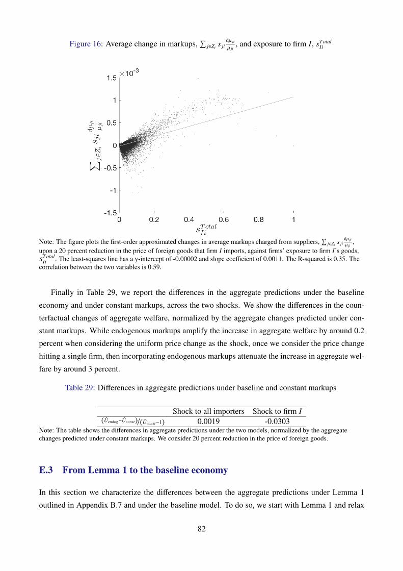
Figure 16: Average change in markups,∑
j∈Zis ji
dµ ji
µ ji, and exposure to firm I, sTotal
Ii
Note: The figure plots the first-order approximated changes in average markups charged from suppliers,∑
j∈Zis ji
dµ ji
µ ji,
upon a 20 percent reduction in the price of foreign goods that firm I imports, against firms’ exposure to firm I’s goods,sTotal
Ii . The least-squares line has a y-intercept of -0.00002 and slope coefficient of 0.0011. The R-squared is 0.35. Thecorrelation between the two variables is 0.59.
Finally in Table 29, we report the differences in the aggregate predictions under the baseline
economy and under constant markups, across the two shocks. We show the differences in the coun-
terfactual changes of aggregate welfare, normalized by the aggregate changes predicted under con-
stant markups. While endogenous markups amplify the increase in aggregate welfare by around 0.2
percent when considering the uniform price change as the shock, once we consider the price change
hitting a single firm, then incorporating endogenous markups attenuate the increase in aggregate wel-
fare by around 3 percent.
Table 29: Differences in aggregate predictions under baseline and constant markups
Shock to all importers Shock to firm I(Uendog−Uconst)/(Uconst−1) 0.0019 -0.0303
Note: The table shows the differences in aggregate predictions under the two models, normalized by the aggregatechanges predicted under constant markups. We consider 20 percent reduction in the price of foreign goods.
E.3 From Lemma 1 to the baseline economy
In this section we characterize the differences between the aggregate predictions under Lemma 1
outlined in Appendix B.7 and under the baseline model. To do so, we start with Lemma 1 and relax
82
the assumptions one by one and also add assumptions needed to make the underlying model closer
to the baseline model.
Table 30 reports the results. In the left column we present the results from Lemma 1, which in-
volved Assumptions 2, 4, and 6. In the next column we first relax Assumption 2, which assumes that
exports are done by the composite final good. The third column further relaxes the Cobb-Douglas
assumption (Assumption 6), and introduce CES production functions and preference using the esti-
mated parameters. Further, in order to compute for nominal wage changes that ensure trade balance
we introduce Assumption 1 of constant measurement errors, εi. The fourth column further relaxes the
perfect competition assumption (Assumption 4). This model is identical to the model under constant
markups introduced in Section 3.4. Finally, we introduce oligopolistic competition, which makes the
model to our baseline model. Comparing the aggregate predictions across models, we find that relax-
ing the Cobb-Douglas assumption and using CES structures makes quantitatively the largest change,
making the prediction of the model closer to that of the baseline model.
Table 30: Aggregate effects from Lemma 1 to baseline model
Lemma 1 Perfect competition, Perfect competition, Constant markups, BaselineCobb-Douglas CES CES
Assumptions 2, 4, and 6 4 and 6 1 and 4 1 1U = E/P 1.129 1.109 1.284 1.272 1.273
E 1 1 1.162 1.149 1.150P/w 0.886 0.902 0.874 0.876 0.876Π NA NA NA 1.329 1.329
Note: This table shows aggregate predictions upon a 20 percent reduction in the price of foreign goods.
E.4 Proposition 1, with different values of σ
Table 31 reports the change in aggregate welfare predicted as in Proposition 1 outlined in Appendix
B.7. We show results when we feed in no shock, pF = 1, and 20 percent reduction in the foreign
price, pF . For the common CES parameter σ, we use three different values: the estimates values for
σ, ρ, and η.
Notice that even when we feed in no shock, Proposition 1 predicts declines in welfare when
we feed in the data. When pF = 1, equation (29) becomes∑
ipiqi(sli+sFi)E+Exports , which should equal to 1
under the assumptions for the Proposition and the trade balance condition. However, since aggregate
expenditure is larger than the sum of labor costs,∑
ipiqi(sli+sFi)E+Exports in the data is around 0.919. Therefore
the change in aggregate welfare is biased downwards under Proposition 1 when one feeds in the data.
83
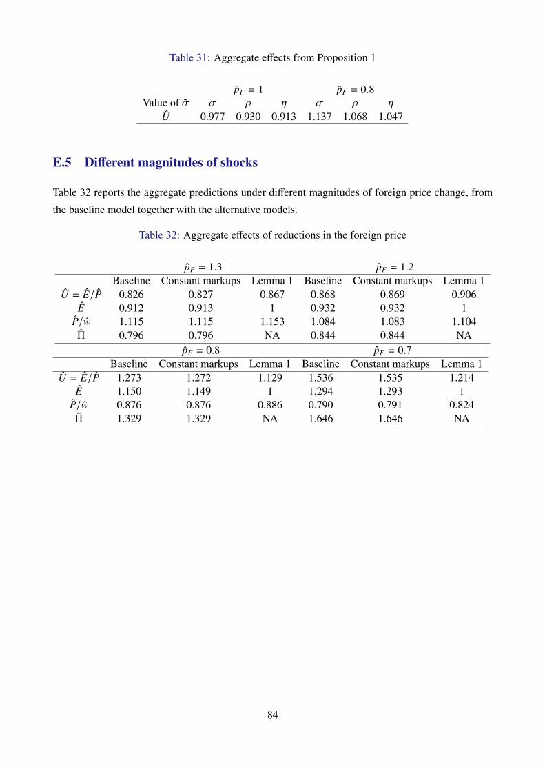
Table 31: Aggregate effects from Proposition 1
pF = 1 pF = 0.8Value of σ σ ρ η σ ρ η
U 0.977 0.930 0.913 1.137 1.068 1.047
E.5 Different magnitudes of shocks
Table 32 reports the aggregate predictions under different magnitudes of foreign price change, from
the baseline model together with the alternative models.
Table 32: Aggregate effects of reductions in the foreign price
pF = 1.3 pF = 1.2Baseline Constant markups Lemma 1 Baseline Constant markups Lemma 1
U = E/P 0.826 0.827 0.867 0.868 0.869 0.906E 0.912 0.913 1 0.932 0.932 1
P/w 1.115 1.115 1.153 1.084 1.083 1.104Π 0.796 0.796 NA 0.844 0.844 NA
pF = 0.8 pF = 0.7Baseline Constant markups Lemma 1 Baseline Constant markups Lemma 1
U = E/P 1.273 1.272 1.129 1.536 1.535 1.214E 1.150 1.149 1 1.294 1.293 1
P/w 0.876 0.876 0.886 0.790 0.791 0.824Π 1.329 1.329 NA 1.646 1.646 NA
84
NBB WORKING PAPER No. 363 – JANUARY 2019 85
NATIONAL BANK OF BELGIUM - WORKING PAPERS SERIES
The Working Papers are available on the website of the Bank: http://www.nbb.be.
317. “An estimated two-country EA-US model with limited exchange rate pass-through”, by G. de Walque,Ph. Jeanfils, T. Lejeune, Y. Rychalovska and R. Wouters, Research series, March 2017.
318. Using bank loans as collateral in Europe: The role of liquidity and funding purposes”, by F. Koulischer andP. Van Roy, Research series, April 2017.
319. “The impact of service and goods offshoring on employment: Firm-level evidence”, by C. Ornaghi,I. Van Beveren and S. Vanormelingen, Research series, May 2017.
320. “On the estimation of panel fiscal reaction functions: Heterogeneity or fiscal fatigue?”, by G. Everaert andS. Jansen, Research series, June 2017.
321. “Economic importance of the Belgian ports: Flemish maritime ports, Liège port complex and the port ofBrussels - Report 2015”, by C. Mathys, Document series, June 2017.
322. “Foreign banks as shock absorbers in the financial crisis?”, by G. Barboni, Research series, June 2017.323. “The IMF and precautionary lending: An empirical evaluation of the selectivity and effectiveness of the
flexible credit line”, by D. Essers and S. Ide, Research series, June 2017.324. “Economic importance of air transport and airport activities in Belgium – Report 2015”, by S. Vennix,
Document series, July 2017.325. “Economic importance of the logistics sector in Belgium”, by H. De Doncker, Document series, July 2017.326. “Identifying the provisioning policies of Belgian banks”, by E. Arbak, Research series, July 2017.327. “The impact of the mortgage interest and capital deduction scheme on the Belgian mortgage market”, by
A. Hoebeeck and K. Inghelbrecht, Research series, September 2017.
328. “Firm heterogeneity and aggregate business services exports: Micro evidence from Belgium, France,Germany and Spain”, by A. Ariu, E. Biewen, S. Blank, G. Gaulier, M.J. González, Ph. Meinen, D. Mirza,C. Martín and P. Tello, Research series, September 2017.
329. “The interconnections between services and goods trade at the firm-level”, by A. Ariu, H. Breinlichz,G. Corcosx, G. Mion, Research series, October 2017.
330. “Why do manufacturing firms produce services? Evidence for the servitization paradox in Belgium”, byP. Blanchard, C. Fuss and C. Mathieu, Research series, November 2017.
331. “Nowcasting real economic activity in the euro area: Assessing the impact of qualitative surveys”, byR. Basselier, D. de Antonio Liedo and G. Langenus, Research series, December 2017.
332. “Pockets of risk in the Belgian mortgage market: Evidence from the Household Finance and ConsumptionSurvey (HFCS)”, by Ph. Du Caju, Research series, December 2017.
333. “The employment consequences of SMEs’ credit constraints in the wake of the great recession” byD. Cornille, F. Rycx and I. Tojerow, Research series, December 2017.
334. “Exchange rate movements, firm-level exports and heterogeneity”, by A. Berthou and E. Dhyne, Researchseries, January 2018.
335 “Nonparametric identification of unobserved technological heterogeneity in production”, by L. Cherchye,T. Demuynck, B. De Rock and M. Verschelde, Research series, February 2018.
336 “Compositional changes in aggregate productivity in an era of globalisation and financial crisis”, by C. Fussand A. Theodorakopoulos, Research series, February 2018.
337. “Decomposing firm-product appeal: How important is consumer taste?”, by B. Y. Aw, Y. Lee andH. Vandenbussche, Research series, March 2018.
338 “Sensitivity of credit risk stress test results: Modelling issues with an application to Belgium”, byP. Van Roy, S. Ferrari and C. Vespro, Research series, March 2018.
339. “Paul van Zeeland and the first decade of the US Federal Reserve System: The analysis from a Europeancentral banker who was a student of Kemmerer”, by I. Maes and R. Gomez Betancourt, Research series,March 2018.
340. “One way to the top: How services boost the demand for goods”, by A. Ariu, F. Mayneris and M. Parenti,Research series, March 2018.
341 “Alexandre Lamfalussy and the monetary policy debates among central bankers during the Great Inflation”,by I. Maes and P. Clement, Research series, April 2018.
342. “The economic importance of the Belgian ports: Flemish maritime ports, Liège port complex and the portof Brussels – Report 2016”, by F. Coppens, C. Mathys, J.-P. Merckx, P. Ringoot and M. Van Kerckhoven,Document series, April 2018.
343. “The unemployment impact of product and labour market regulation: Evidence from European countries”,by C. Piton, Research series, June 2018.
344. “Trade and domestic production networks”, by F. Tintelnot, A. Ken Kikkawa, M. Mogstad, E. Dhyne,Research series, September 2018.
86 NBB WORKING PAPER No. 363 – JANUARY 2019
345. “Review essay: Central banking through the centuries”, by I. Maes, Research series, October 2018.346. “IT and productivity: A firm level analysis”, by E. Dhyne, J. Konings, J. Van den Bosch, S. Vanormelingen,
Research series, October 2018.347. “Identifying credit supply shocks with bank-firm data: methods and applications”, by H. Degryse,
O. De Jonghe, S. Jakovljević, Klaas Mulier, Glenn Schepens, Research series, October 2018.348. “Can inflation expectations in business or consumer surveys improve inflation forecasts?”, by R. Basselier,
D. de Antonio Liedo, J. Jonckheere and G. Langenus, Research series, October 2018.349. “Quantile-based inflation risk models”, by E. Ghysels, L. Iania and J. Striaukas, Research series,
October 2018.350. “International food commodity prices and missing (dis)inflation in the euro area”, by G. Peersman,
Research series, October 2018.351. “Pipeline pressures and sectoral inflation dynamics”, by F. Smets, J. Tielens and J. Van Hove, Research
series, October 2018.352. “Price updating in production networks”, by C. Duprez and G. Magerman, Research series, October 2018.353. “Dominant currencies. How firms choose currency invoicing and why it matters”, by M. Amiti, O. Itskhoki
and J. Konings, Research series, October 2018.354. “Endogenous forward guidance”, by B. Chafwehé, R. Oikonomou, R. Priftis and L. Vogel, Research series,
October 2018.355. “Is euro area Iowflation here to stay? Insights from a time-varying parameter model with survey data”, by
A. Stevens and J. Wauters, Research series, October 2018.356. “A price index with variable mark-ups and changing variety”, by T. Demuynck and M. Parenti, Research
series, October 2018.357. “Markup and price dynamics: Linking micro to macro”, by J. De Loecker, C. Fuss and J. Van Biesebroeck,
Research series, October 2018.358. “Productivity, wages and profits: Does firms’ position in the value chain matter?”, by B. Mahy, F. Rycx,
G. Vermeylen and M. Volral, Research series, October 2018.359. “Upstreamness, social upgrading and gender: Equal benefits for all?”, by N. Gagliardi, B. Mahy and
F. Rycx, Research series, December 2018.360. “A macro-financial analysis of the corporate bond market”, by H. Dewachter, L. Iania, W. Lemke and
M. Lyrio, Research series, December 2018.361. “Some borrowers are more equal than others: Bank funding shocks and credit reallocation”, by
O. De Jonghe, H. Dewachter, K. Mulier, S. Ongena and G. Schepens, Research series, December 2018.362. “The origins of firm heterogeneity: A production network approach”, by A. B. Bernard, E. Dhyne,
G. Magerman, K. Manova and A. Moxnes, Research series, January 2019.363. “Imperfect competition in firm-to-firm trade”, by A. Ken Kikkawa, G. Magerman and E. Dhyne, Research
series, January 2019.
© Illustrations : National Bank of Belgium
Layout : Analysis and Research Group Cover : NBB AG – Prepress & Image
Published in January 2019
Editor
Pierre WunschGovernor of the National Bank of Belgium
National Bank of Belgium Limited liability company RLP Brussels – Company’s number : 0203.201.340 Registered office : boulevard de Berlaimont 14 – BE -1000 Brussels www.nbb.be


![Level 5 Economics: Theory of the Firm [3] Economic Principles Economic Principles Economic Environment Economic Environment Imperfect Competition Imperfect](https://cdn.vdocument.in/doc/165x107/56649e755503460f94b76c5f/level-5-economics-theory-of-the-firm-3-economic-principles-economic-principles.jpg)