
1
INDEX NUMBER THEORY AND MEASUREMENT ECONOMICS
By W.E. Diewert, January, 2015.
CHAPTER 7: The Use of Annual Weights in a Monthly Index
1. The Lowe Index with Monthly Prices and Annual Base Year Quantities
It is now necessary to discuss a major practical problem with the theory of bilateral
indexes that we have been discussing in earlier chapters. Recall that the Lowe (1823)
index was defined by equation (19) in chapter 1 as follows:
(1) PLo(p0,p
1,q) p
1q / p
0q.
The Lowe index can be written in expenditure share form as follows:
(2) PLo(p0,p
1,q) n=1
N pn
1qn / n=1
N pn
0qn
= n=1N (pn
1/pn
0) sn
where the (hypothetical) hybrid expenditure shares sn corresponding to the quantity
weights vector q are defined by:1
(3) sn pn0qn / n=1
N pn
0qn for n = 1,…,N.
Up to now, it has been assumed that the quantity vector q (q1,q2,…,qN) that appeared in
the definition of the Lowe index, PLo(p0,p
1,q), is either the base period quantity vector q
0
or the current period quantity vector q1 or an average of these two quantity vectors. In
fact, in terms of actual statistical agency practice, the quantity vector q is usually taken to
be an annual quantity vector that refers to a base year, b say, that is prior to the base
period for the prices, period 0. Typically, a statistical agency will produce a Consumer
Price Index at a monthly or quarterly frequency but for the sake of definiteness, a
monthly frequency will be assumed in what follows. Thus a typical price index will have
the form PLo(p0,p
t,q
b), where p
0 is the price vector pertaining to the base period month for
prices, month 0, pt is the price vector pertaining to the current period month for prices,
month t say, and qb is a reference basket quantity vector that refers to the base year b,
which is equal to or prior to month 0.2 Note that this Lowe index PLo(p
0,p
t,q
b) is not a
true Laspeyres index (because the annual quantity vector qb is not equal to the monthly
quantity vector q0 in general).
3
1 Fisher (1922; 53) used the terminology “weighted by a hybrid value” while Walsh (1932; 657) used the
term “hybrid weights”. 2 Month 0 is called the price reference period and year b is called the weight reference period.
3 Triplett (1981; 12) defined the Lowe index, calling it a Laspeyres index, and calling the index that has the
weight reference period equal to the price reference period, a pure Laspeyres index. However, Balk (1980;
69) asserted that although the Lowe index is of the fixed base type, it is not a Laspeyres price index.
Triplett also noted the hybrid share representation for the Lowe index defined by (2) and (3) above.
Triplett noted that the ratio of two Lowe indices using the same quantity weights was also a Lowe index.
Baldwin (1990; 255) called the Lowe index an annual basket index.
2
The question is: why do statistical agencies not pick the reference quantity vector q in the
Lowe formula to be the monthly quantity vector q0 that pertains to transactions in month
0 (so that the index would reduce to an ordinary Laspeyres price index)? There are two
main reasons why this is not done:
Most economies are subject to seasonal fluctuations and so picking the quantity
vector of month 0 as the reference quantity vector for all months of the year
would not be representative of transactions made throughout the year.
Monthly household quantity or expenditure weights are usually collected by the
statistical agency using a household expenditure survey with a relatively small
sample. Hence the resulting weights are usually subject to very large sampling
errors and so standard practice is to average these monthly expenditure or
quantity weights over an entire year (or in some cases, over several years), in an
attempt to reduce these sampling errors.
The index number problems that are caused by seasonal monthly weights will be studied
in more detail in a later chapter. For now, it can be argued that the use of annual weights
in a monthly index number formula is simply a method for dealing with the seasonality
problem.4
One problem with using annual weights corresponding to a perhaps distant year in the
context of a monthly Consumer Price Index must be noted at this point: if there are
systematic (but divergent) trends in commodity prices and households increase their
purchases of commodities that decline (relatively) in price and decrease their purchases
of commodities that increase (relatively) in price, then the use of distant quantity weights
will tend to lead to an upward bias in this Lowe index compared to one that used more
current weights, as will be shown below. This observation suggests that statistical
agencies should strive to get up to date weights on an ongoing basis.
It is useful to explain how the annual quantity vector qb could be obtained from monthly
expenditures on each commodity during the chosen base year b. Let the month m
expenditure of the reference population in the base year b for commodity i be vib,m
and let
the corresponding price and quantity be pib,m
and qib,m
respectively. Of course, value,
price and quantity for each commodity are related by the following equations:
(4) vnb,m
= pnb,m
qnb,m
; n = 1,…,N ; m = 1,…,12.
For each commodity n, the annual total, qnb can be obtained by price deflating monthly
values and summing over months in the base year b as follows:
(5) qnb = m=1
12 vn
b,m / pn
b,m = m=1
12 qn
b,m ; n = 1,…,N
4 In fact, the use of the Lowe index PLo(p
0,p
t,q
b) in the context of seasonal commodities corresponds to
Bean and Stine’s (1924; 31) Type A index number formula. Bean and Stine made 3 additional suggestions
for price indexes in the context of seasonal commodities. Their contributions will be evaluated in a later
chapter.
3
where (4) was used to derive the second equation in (5). In practice, the above equations
will be evaluated using aggregate expenditures over closely related commodities and the
price pnb,m
will be the month m price index for this elementary commodity group n in
year b relative to the first month of year b.
For some purposes, it is also useful to have annual prices by commodity to match up with
the annual quantities defined by (5). Following national income accounting conventions,
a reasonable5 price pn
b to match up with the annual quantity qn
b is the value of total
consumption of commodity n in year b divided by qnb. Thus we have:
(6) pnb m=1
12 vn
b,m /qn
b n = 1,…,N
= m=112
vnb,m
/[m=112
vnb,m
/ pnb,m
] using (5)
= [m=112
snb,m
(pnb,m
)1
]1
where the share of annual expenditure on commodity n in month m of the base year is
(7) snb,m
vnb,m
/k=112
vnb,k
; n = 1,…,N ; m = 1,…,12.
Thus the annual base year price for commodity n, pnb, turns out to be a monthly
expenditure weighted harmonic mean of the monthly prices for commodity n in the base
year, pnb,1
, pnb,2
,…, pnb,12
.
Using the annual commodity prices for the base year defined by (6), a vector of these
prices can be defined as pb [p1
b,…,pN
b]. Using this definition, the Lowe index
PLo(p0,p
t,q
b) can be expressed as a ratio of two Laspeyres indexes where the price vector
pb plays the role of base period prices in each of the two Laspeyres indexes:
(8) PLo(p0,p
t,q
b) p
tq
b /p
0q
b
= [ptq
b /p
bq
b]/[p
0q
b /p
bq
b]
= PL(pb,p
t,q
b)/PL(p
b,p
0,q
b)
= n=1N (pn
t/pn
b) sn
b /n=1
N (pn
0/pn
b) sn
b
where the Laspeyres formula PL was defined in Chapter 1. Thus the above equation
shows that the Lowe monthly price index comparing the prices of month 0 to those of
month t using the quantities of base year b as weights, PLo(p0,p
t,q
b), is equal to the
Laspeyres index that compares the prices of month t to those of year b, PL(pb,p
t,q
b),
divided by the Laspeyres index that compares the prices of month 0 to those of year b,
PL(pb,p
0,q
b). Note that the Laspeyres index in the numerator can be calculated if the base
5 Hence these annual commodity prices are essentially unit value prices. Under conditions of high
inflation, the annual prices defined by (6) may no longer be “reasonable” or representative of prices during
the entire base year because the expenditures in the final months of the high inflation year will be
somewhat artificially blown up by general inflation. Under these conditions, the annual prices and annual
commodity expenditure shares should be interpreted with caution. For more on dealing with situations
where there is high inflation within a year, see Hill (1996).

4
year commodity expenditure shares, snb, are known along with the price ratios that
compare the prices of commodity n in month t, pnt, with the corresponding annual
average prices in the base year b, pnb. The Laspeyres index in the denominator can be
calculated if the base year commodity expenditure shares, snb, are known along with the
price ratios that compare the prices of commodity n in month 0, pn0, with the
corresponding annual average prices in the base year b, pnb.
There is another convenient formula for evaluating the Lowe index, PLo(p0,p
t,q
b), and that
is to use the hybrid weights formula, (2). In the present context, the formula becomes:
(9) PLo(p0,p
t,q
b) n=1
N pn
tqn
b / n=1
N pn
0qn
b
= n=1N (pn
t/pn
0) sn
0b
where the (hypothetical) hybrid expenditure shares sn0b
corresponding to the quantity
weights vector q are defined by:6
(10) sn0b
pn0qn
b / n=1
N pn
0qn
b for n = 1,…,N
= pnbqn
b(pn
0/pn
b)/j=1
N pj
bqj
b(pj
0/pj
b).
The second equation in (10) shows how the base year expenditures on commodity n,
pnbqn
b, can be multiplied by the commodity price indexes, pn
0/pn
b, in order to calculate the
hybrid shares.
There is one additional formula for the Lowe index, PLo(p0,p
t,q
b), that will be exhibited.
Note that the Laspeyres decomposition of the Lowe index defined by the fourth line in
(8) involves the very long term price relatives, pnt/pn
b, which compare the prices in month
t, pnt, with the possibly distant base year prices, pn
b, and that the hybrid share
decomposition of the Lowe index defined by the second line in (9) involves the long term
monthly price relatives, pit/pi
0, which compare the prices in month t, pi
t, with the base
month prices, pi0. Both of these formulae are not satisfactory in practice due to the
problem of sample attrition: each month, a substantial fraction of commodities disappears
from the marketplace and thus it is useful to have a formula for updating the previous
month’s price index using just month over month price relatives. In other words, long
term price relatives disappear at a rate that is too large in practice to base an index
number formula on their use. The Lowe index for month t+1, PLo(p0,p
t+1,q
b), can be
written in terms of the Lowe index for month t, PLo(p0,p
t,q
b), and an updating factor as
follows:
(11) PLo(p0,p
t+1,q
b) p
t+1q
b /p
0q
b
= [ptq
b /p
0q
b][p
t+1q
b /p
tq
b]
= PLo(p0,p
t,q
b)[p
t+1q
b /p
tq
b]
= PLo(p0,p
t,q
b)[n=1
N sn
tb(pn
t+1/pn
t)]
6 Fisher (1922; 53) used the terminology “weighted by a hybrid value” while Walsh (1932; 657) used the
term “hybrid weights”.
5
where the hybrid weights sntb
are defined by
(12) sntb
pntqn
b/k=1
N pk
tqk
b ; n = 1,…,N.
Thus the required updating factor, going from month t to month t+1, is the chain link
index n=1N sn
tb (pn
t+1/pn
t), which uses the hybrid share weights sn
tb corresponding to
month t and base year b.
It should be noted that the month t hybrid shares, can be constructed from the previous
month’s hybrid shares, snt1,b
pnt1
qnb/k=1
N pk
t1qk
b, by using the following updating
formula:
(13) sntb
pntqn
b/k=1
N pk
tqk
b ; n = 1,…,N
= pnt1
qnb(pn
t/pn
t1)/j=1
N pj
tqj
b
= [pnt1
qnb(pn
t/pn
t1)/p
t1q
b] /[j=1
N pj
tqj
b/p
t1q
b]
= snt1,b
(pnt/pn
t1)/[j=1
N pj
tqj
b/p
t1q
b]
= snt1,b
(pnt/pn
t1)/[j=1
N (pj
t/pj
t1)pj
t1qj
b/p
t1q
b]
= snt1,b
(pnt/pn
t1)/[j=1
N (pj
t/pj
t1)sj
t1,b]
= (pnt/pn
t1)sn
t1,b/[j=1
N (pj
t/pj
t1)sj
t1,b].
Formula (13) can be used recursively until we get to t = 1, when (13) becomes:
(14) sn1,b
pn1qn
b/k=1
N pk
1qk
b ; n = 1,…,N
= (pn1/pn
0)sn
0,b/[j=1
N (pj
1/pj
0)sj
0,b].
The hybrid shares, sn0,b
, that use the components of the base year quantity vector qb and
the base month price vector p0, can be constructed from base year expenditures, pn
bqn
b,
and the “mixed” month to year price relatives, (pn0/pn
b), using formula (10) above. Thus
we have developed a complete set of “practical” updating formulae.
The Lowe index PLo(p0,p
t,q
b) can be regarded as an approximation to the ordinary
Laspeyres index, PL(p0,p
t,q
0), that compares the prices of the base month 0, p
0, to those of
month t, pt, using the quantity vector of month 0, q
0, as weights. It turns out that there is
a relatively simple formula that relates these two indexes. However, before we present
this formula, we digress momentarily and develop a relationship between the Paasche and
Laspeyres price indexes. It turns out that we can adapt this methodology to the problem
of relating the Lowe index to the Laspeyres index.
2. The Bortkiewicz Decomposition between the Paasche and Laspeyres Indexes
In this section, we will develop a relationship between the ordinary Paasche and
Laspeyres price indexes.7 In order to explain this formula, it is first necessary to make a
few definitions. Define the nth price relative between month 0 and month t as
7 This relationship was originally discovered by Bortkiewicz (1923; 374-375).

6
(15) rn pnt/pn
0 ; n = 1,…,N.
The ordinary Laspeyres price index, relating the prices of month 0 to those of month t,
can be defined as a weighted average of these price relatives as follows:
(16) PL(p0,p
t,q
0) n=1
N sn
0 (pn
t/pn
0)
= n=1N sn
0 rn using (15)
r*
where the month 0 expenditure shares sn0 are defined as follows:
(17) sn0 pn
0qn
0/k=1
N pk
0qk
0 ; n = 1,…,N.
Define the nth quantity relative tn as the ratio of the quantity of commodity n used in the
month t, qnt, to the quantity used in month 0, qn
0, as follows:
(18) tn qnt/qn
0 ; n = 1,…,N.
The Laspeyres quantity index, QL(q0,q
t,p
0), that compares quantities in month t, q
t, to the
corresponding quantities in month 0, q0, using the prices of month 0, p
0, as weights can
be defined as a weighted average of the quantity ratios tn as follows:
(19) QL(q0,q
t,p
0) p
0q
t /p
0q
0
= n=1N sn
0 tn using (17) and (18)
t*.
Before we compare the Paasche and Laspeyres price indexes, we need to undertake a
preliminary computation using the above definitions of rn and tn:
(20) Cov(r,t,s0) n=1
N (rn r*)(tn t*)sn
0
= n=1N rntnsn
0 n=1
N rnt*sn
0 n=1
N r*tnsn
0 + n=1
N r*t*sn
0
= n=1N rntnsn
0 t*n=1
N rnsn
0 r*n=1
N tnsn
0 + r*t*n=1
N sn
0
= n=1N rntnsn
0 t*n=1
N rnsn
0 r*n=1
N tnsn
0 + r*t* using n=1
N sn
0 = 1
= n=1N rntnsn
0 t*r* r*t* + r*t* using (16) and (19)
= n=1N rntnsn
0 t*r*.
Note that Cov(r,t,s0) can be interpreted as a weighted covariance between the vector of
price relatives, r [r1,…,rN], and the vector of quantity relatives, t [t1,…,tN], using the
base period vector of expenditure shares, s0 [s1
0,…,sN
0], as weights. More explicitly, let
r and t be discrete random variables that take on the N values rn and tn respectively. Let
sn0 be the joint probability that r = rn and t = tn for n = 1,…,N and let the joint probability
be 0 if r = ri and t = tj where i j. It can be verified that Cov(r,t,s0) defined in the first

7
line of (20) is the covariance between the price relatives rn and the corresponding quantity
relatives tn. This covariance can be converted into a correlation coefficient.8
Now we are ready to exhibit von Bortkiewicz’s formula relating the Paasche and
Laspeyres indexes. The Paasche index, PP(p0,p
t,q
t), that compares the prices of the base
month 0, p0, to those of month t, p
t, using the quantity vector of month t, q
t, as a
weighting vector is defined as follows:
(21) PP(p0,p
t,q
t) n=1
N pn
tqn
t / n=1
N pn
0qn
t
= n=1N rntn pn
0qn
0 / n=1
N tn pn
0qn
0 using definitions (15) and (18)
= [n=1N rntn pn
0qn
0/p
0q
0]/[n=1
N tn pn
0qn
0/p
0q
0]
= n=1N rntn sn
0 /n=1
N tn sn
0 using definitions (17)
= n=1N rntn sn
0 /t* using definition (19)
= [{n=1N (rn r*)(tn t*)sn
0} + r*t*]/t* using (20)
= [n=1N (rn r*)(tn t*)sn
0/t*] + r*
= [n=1N (rn r*)(tn t*)sn
0/QL(q
0,q
t,p
0)] + PL(p
0,p
t,q
0)
using (16) and (19).
Subtracting PL(p0,p
t,q
0) from both sides of (21) leads to the following relationship
between the Paasche and Laspeyres price indexes:
(22) PP(p0,p
t,q
t) PL(p
0,p
t,q
0) = n=1
N (rn r*)(tn t*)sn
0/QL(q
0,q
t,p
0)
= Cov(r,t,s0)/QL(q
0,q
t,p
0).
Thus the difference between the Paasche and Laspeyres price indexes relating the prices
of period 0 to those of period t is equal to the covariance between the relative price and
relative quantity vectors, Cov(r,t,s0), divided by the Laspeyres quantity index,
QL(q0,q
t,p
0). Usually, this covariance will be negative for most value aggregates
9 so that
usually the Paasche index will be less than the corresponding Laspeyres index.
In the following section, we will develop a similar relationship between the Lowe and
Laspeyres indexes using the same technique as was used by Bortkiewicz.
3. The Relationship between the Lowe, Laspeyres and Paasche Indexes
We shall use the same notation for the long term monthly price relatives rn pnt/pn
0 that
was used in the previous section so that (15)-(17) are still used in the present section.
However, we shall change the definition of the tn in the previous section in order to relate
the base year annual quantities qnb to the base month quantities qn
0:
(23) tn qnb/qn
0 ; n = 1,…,N.
8 See Bortkiewicz (1923; 374-375) for the first application of this correlation coefficient decomposition
technique. 9 As we shall see later, this corresponds to the situation where demander substitution effects outweigh
supplier substitution effects.

8
We also define a new Laspeyres quantity index QL(q0,q
b,p
0), which compares the base
year quantity vector qb to the base month quantity vector q
0, using the price weights of
the base month p0, as follows:
(24) QL(q0,q
b,p
0) p
0q
b/p
0q
0
= n=1N pn
0qn
b / n=1
N pn
0qn
0
= n=1N pn
0qn
0 (qn
b/qn
0) / n=1
N pn
0qn
0
= n=1N sn
0 (qn
b/qn
0) using definitions (17)
= n=1N sn
0(tn) using definitions (23)
t*.
Using definition (9), the Lowe index comparing the prices in month t to those of month 0,
using the quantity weights of the base year b, is equal to:
(25) PLo(p0,p
t,q
b) n=1
N pn
tqn
b / n=1
N pn
0qn
b
= n=1N pn
t tnqn
0 / n=1
N pn
0 tnqn
0 using definitions (23)
= n=1N rnpn
0 tnqn
0 / n=1
N pn
0 tnqn
0 using definitions (15)
= [n=1N rntn pn
0qn
0/p
0q
0] / [n=1
N tnpn
0qn
0/p
0q
0]
= n=1N rntn sn
0 / n=1
N tn sn
0 using definitions (17)
= n=1N rntn sn
0 / t* using (24)
= [{n=1N (rn r*)(tn t*)sn
0} + t*r*]/t* using the identity (20)
= [n=1N (rn r*)(tn t*)sn
0/t*] + r*
= [n=1N (rn r*)(tn t*)sn
0/t*] + PL(p
0,p
t,q
0) using definition (16)
= [Cov(r,t,s0)/QL(q
0,q
b,p
0)] + PL(p
0,p
t,q
0)
where the last equality follows using definitions (20) and (24). Subtracting the Laspeyres
price index relating the prices of month t to those of month 0, PL(p0,p
t,q
0), from both
sides of (25) leads to the following relationship of this monthly Laspeyres price index to
its Lowe counterpart:
(26) PLo(p0,p
t,q
b) PL(p
0,p
t,q
0) = n=1
N (rn r*)(tn t*)sn
0/QL(q
0,q
b,p
0)
= Cov(r,t,s0)/QL(q
0,q
b,p
0).
Thus the difference between the Lowe and Laspeyres price indexes relating the prices of
period 0 to those of period t is equal to the covariance between the relative price and
relative quantity vectors, Cov(r,t,s0), divided by the Laspeyres quantity index,
QL(q0,q
b,p
0). Thus (26) tells us that the Lowe price index using the quantities of year b as
weights, PLo(p0,p
t,q
b), is equal to the usual Laspeyres index using the quantities of month
0 as weights, PL(p0,p
t,q
0), plus a covariance term n=1
N (rn r*)(tn t*)sn
0 between the
long term monthly price relatives rn pnt/pn
0 and the quantity relatives tn qn
b/qn
0 (which
are equal to the base year quantities qnb
divided by the base month quantities qn0), divided
by the Laspeyres quantity index QL(q0,q
b,p
0) between month 0 and base year b.
9
Formula (26) shows that the Lowe price index will coincide with the Laspeyres price
index if the covariance or correlation between the month 0 to t price relatives rn pnt/pn
0
and the month 0 to year b quantity relatives tn qnb/qn
0 is zero. Note that this covariance
will be zero under three different sets of conditions:
If the month t prices are proportional to the month 0 prices so that all rn equal r*;
If the base year b quantities are proportional to the month 0 quantities so that all tn
equal t*;
If the distribution of the relative prices rn is independent of the distribution of the
relative quantities tn.
The first two conditions are unlikely to hold empirically but the third is possible, at least
approximately, if consumers do not systematically change their purchasing habits in
response to changes in relative prices.
If the covariance in (26) is negative, then the Lowe index will be less than the Laspeyres
and finally, if the covariance is positive, then the Lowe index will be greater than the
Laspeyres index. Although the sign and magnitude of the covariance term, n=1N (rn
r*)(tn t*)sn0, is ultimately an empirical matter, it is possible to make some reasonable
conjectures about its likely sign. If the base year b precedes the price reference month 0
and there are long term trends in prices, then it is likely that this covariance is positive
and hence the Lowe index will exceed the corresponding Laspeyres price index10
; i.e.,
(27) PLo(p0,p
t,q
b) > PL(p
0,p
t,q
0).
To see why this covariance is likely to be positive, suppose that there is a long term
upward trend in the price of commodity n so that rn r* (pnt/pn
0) r* is positive. With
normal consumer substitution responses11
, qnt/qn
0 less an average quantity change of this
type is likely to be negative, or, upon taking reciprocals, qn0/qn
t less an average quantity
change of this (reciprocal) type is likely to be positive. But if the long term upward trend
in prices has persisted back to the base year b, then tn t* (qnb/qn
0) t* is also likely to
be positive. Hence, the covariance will be positive under these circumstances.
Moreover, the more distant is the base year b from the base month 0, the bigger the
residuals tn t* will likely be and the bigger will be the positive covariance. Similarly,
the more distant is the current period month t from the base period month 0, the bigger
the residuals rn r* will likely be and the bigger will be the positive covariance. Thus
under the assumptions that there are long term trends in prices and normal consumer
10
It is also necessary to assume that households have normal substitution effects in response to these long
term trends in prices; i.e., if a commodity increases (relatively) in price, its consumption will decline
(relatively) and if a commodity decreases relatively in price, its consumption will increase relatively. 11
Walsh (1901; 281-282) was well aware of consumer substitution effects as can be seen in the following
comment which noted the basic problem with a fixed basket index that uses the quantity weights of a single
period: “The argument made by the arithmetic averagist supposes that we buy the same quantities of every
class at both periods in spite of the variation in their prices, which we rarely, if ever, do. As a rough
proposition, we –a community –generally spend more on articles that have risen in price and get less of
them, and spend less on articles that have fallen in price and get more of them.”
10
substitution responses, the Lowe index will usually be greater than the corresponding
Laspeyres index.
Recall relationship (22) in the previous section, which related the difference between the
Paasche and Laspeyres price indexes, PP(p0,p
t,q
t) and PL(p
0,p
t,q
0), to the covariance term,
n=1N (rn r*)(tn t*)sn
0, where the quantity relatives tn qn
t/qn
0 were defined by (18).
Although the sign and magnitude of the covariance term in (22), n=1N (rn r*)(tn
t*)sn0, is again an empirical matter, it is possible to make a reasonable conjecture about
its likely sign. If there are long term trends in prices and consumers respond normally to
price changes in their purchases, then it is likely that that this covariance is negative and
hence the Paasche index will be less than the corresponding Laspeyres price index; i.e.,
(28) PP(p0,p
t,q
t) < PL(p
0,p
t,q
0).
To see why this covariance is likely to be negative, suppose that there is a long term
upward trend in the price of commodity n12
so that rn r* (pnt/pn
0) r* is positive.
With normal consumer substitution responses, qnt/qn
0 less an average quantity change of
this type is likely to be negative. Hence tn t* (qnt/qn
0) t* is likely to be negative.
Thus, the covariance will be negative under these circumstances. Moreover, the more
distant is the base month 0 from the current month t, the bigger in magnitude the
residuals tn t* will likely be and the bigger in magnitude will be the negative
covariance.13
Similarly, the more distant is the current period month t from the base
period month 0, the bigger the residuals rn r* will likely be and the bigger in magnitude
will be the covariance. Thus under the assumptions that there are long term trends in
prices and normal consumer substitution responses, the Laspeyres index will be greater
than the corresponding Paasche index, with the divergence likely growing as month t
becomes more distant from month 0.
Putting the arguments in the three previous paragraphs together, it can be seen that under
the assumptions that there are long term trends in prices and normal consumer
substitution responses, the Lowe price index between months 0 and t will exceed the
corresponding Laspeyres price index which in turn will exceed the corresponding
Paasche price index; i.e., under these hypotheses,
(29) PLo(p0,p
t,q
b) > PL(p
0,p
t,q
0) > PP(p
0,p
t,q
t).
Thus if the long run target price index is an average of the Laspeyres and Paasche
indexes, it can be seen that the Laspeyres index will have an upward bias relative to this
target index and the Paasche index will have a downward bias. In addition, if the base
year b is prior to the price reference month, month 0, then the Lowe index will also have
12
The reader can carry through the argument if there is a long term relative decline in the price of the ith
commodity. The argument required to obtain a negative covariance requires that there be some differences
in the long term trends in prices; i.e., if all prices grow (or fall) at the same rate, we have price
proportionality and the covariance will be zero. 13
However, QL = t* may also be growing in magnitude so the net effect on the divergence between PL and
PP is ambiguous.
11
an upward bias relative to the Laspeyres index and hence also to the target index. The
previous sentence is not good news for statistical agencies that base their consumer price
index on the Lowe index that uses base year quantities for a distant year as weights.
5. The Lowe Index and Midyear Indexes
The discussion in the previous sections assumed that the base year b for quantities
preceded the base month for prices, month 0. However, if the current period month t is
quite distant from the base month 0, then it is possible to collect expenditure information
for a base year b that lies between months 0 and t. If the year b does fall between months
0 and t, then the Lowe index becomes a midyear index.14
It turns out that if the base year
is between monthly periods 0 and t, then the Lowe midyear index no longer has the
upward biases indicated by the inequalities in (29) under the assumption of long term
trends in prices and normal substitution responses by quantities.
We now assume that the base year quantity vector qb corresponds to a year that lies
between months 0 and t. Under the assumption of long term trends in prices and normal
substitution effects so that there are also long term trends in quantities (in the opposite
direction to the trends in prices so that if the nth commodity price is trending up, then the
corresponding nth quantity is trending down), it is likely that the intermediate year
quantity vector will lie between the monthly quantity vectors q0 and q
t. The midyear
Lowe index, PLo(p0,p
t,q
b), and the Laspeyres index going from month 0 to t, PL(p
0,p
t,q
0),
will still satisfy the exact relationship given by equation (26) above. Thus PLo(p0,p
t,q
b)
will equal PL(p0,p
t,q
0) plus the covariance term [n=1
N (rn r*)(tn t*)sn
0 ]/QL(q
0,q
b,p
0),
where QL(q0,q
b,p
0) is the Laspeyres quantity index going from month 0 to base year b.
This covariance term is likely to be negative so that
(30) PLo(p0,p
t,q
b) < PL(p
0,p
t,q
0).
To see why this covariance is likely to be negative, suppose that there is a long term
upward trend in the price of commodity n so that rn r* (pnt/pn
0) r* is positive. With
14
This concept can be traced to Peter Hill (1998; 46): “When inflation has to be measured over a specified
sequence of years, such as a decade, a pragmatic solution to the problems raised above would be to take the
middle year as the base year. This can be justified on the grounds that the basket of goods and services
purchased in the middle year is likely to be much more representative of the pattern of consumption over
the decade as a whole than baskets purchased in either the first or the last years. Moreover, choosing a
more representative basket will also tend to reduce, or even eliminate, any bias in the rate of inflation over
the decade as a whole as compared with the increase in the CoL index.” Thus in addition to introducing the
concept of a midyear index, Hill also introduced the terminology representativity bias. Baldwin (1990;
255-256) also introduced the term representativeness: “Here representativeness [in an index number
formula] requires that the weights used in any comparison of price levels are related to the volume of
purchases in the periods of comparison.” However, this basic idea dates back to Walsh (1901; 104) (1921a;
90). Baldwin (1990; 255) also noted that his concept of representativeness was the same as Drechsler’s
(1973; 19) concept of characteristicity. For additional material on midyear indexes, see Schultz (1999) and
Okamoto (2001). Note that the midyear index concept could be viewed as a close competitor to Walsh’s
(1901; 431) multiyear fixed basket index where the quantity vector was chosen to be an arithmetic or
geometric average of the quantity vectors in the span of periods under consideration.
12
normal consumer substitution responses, qn will tend to decrease relatively over time and
since qnb is assumed to be between qn
0 and qn
t, qn
b/qn
0 less an average quantity change of
this type is likely to be negative. Hence tn t* (qnb/qn
0) t* is likely to be negative.
Thus, the covariance is likely to be negative under these circumstances. Thus under the
assumptions that the quantity base year falls between months 0 and t and that there are
long term trends in prices and normal consumer substitution responses, the Laspeyres
index will normally be larger than the corresponding Lowe midyear index, with the
divergence likely growing as month t becomes more distant from month 0.
It can also be seen that under the above assumptions, the midyear Lowe index is likely to
be greater than the Paasche index between months 0 and t; i.e.,
(31) PLo(p0,p
t,q
b) > PP(p
0,p
t,q
t).
To see why the above inequality is likely to hold, think of qb starting at the month 0
quantity vector q0 and then trending smoothly to the month t quantity vector q
t. When q
b
= q0, the Lowe index PLo(p
0,p
t,q
b) becomes the Laspeyres index PL(p
0,p
t,q
0). When q
b =
qt, the Lowe index PLo(p
0,p
t,q
b) becomes the Paasche index PP(p
0,p
t,q
t). Under the
assumption of trending prices and normal substitution responses to these trending prices,
it was shown earlier that the Paasche index will be less than the corresponding Laspeyres
price index; i.e., that PP(p0,p
t,q
t) was less than PL(p
0,p
t,q
0); recall (22). Thus under the
assumption of smoothly trending prices and quantities between months 0 and t, and
assuming that qb is between q
0 and q
t, we will have
(32) PP(p0,p
t,q
t) < PLo(p
0,p
t,q
b) < PL(p
0,p
t,q
0).
Thus if the base year for the Lowe index is chosen to be in between the base month for the
prices, month 0, and the current month for prices, month t, and there are trends in prices
with corresponding trends in quantities that correspond to normal consumer substitution
effects, then the resulting Lowe index is likely to lie between the Paasche and Laspeyres
indexes going from months 0 to t. If the trends in prices and quantities are smooth, then
choosing the base year half way between periods 0 and t should give a Lowe index that is
approximately half way between the Paasche and Laspeyres indexes and hence will be
very close to an ideal target index between months 0 and t. This basic idea has been
implemented by Okamoto (2001) using Japanese consumer data and he found that the
resulting midyear indexes approximated the corresponding Fisher ideal indexes very
closely. However, the assumption of smooth trends in prices and quantities is necessary
to get this close approximation.
All of the inequalities derived in this chapter rest on the assumption of long term trends in
prices (and corresponding economic responses in quantities). If there are no systematic
long run trends in prices, but only random fluctuations around a common trend in all
prices, then the above inequalities are not valid and the Lowe index using a prior base
year will probably provide a perfectly adequate approximation to both the Paasche and
Laspeyres indices. However, there are some reasons for believing that there are some
long run trends in prices. Some of these reasons are:

13
The computer chip revolution of the past 40 years has led to strong downward
trends in the prices of products that use these chips intensively. As new uses for
chips have been developed over the years, the share of products that are chip
intensive has grown and this implies that what used to be a relatively minor
problem has become a more major problem.
Other major scientific advances have had similar effects. For example, the
invention of fiber optic cable (and lasers) has led to a downward trend in
telecommunications prices as obsolete technologies based on copper wire are
gradually replaced.
Since the end of World War II, there have been a series of international trade
agreements that have dramatically reduced tariffs around the world. These
reductions, combined with improvements in transportation technologies, have led
to a very rapid growth of international trade and remarkable improvements in
international specialization. Manufacturing activities in the more developed
economies have gradually been outsourced to lower wage countries, leading to
deflation in goods prices in most countries around the world. However, many
services cannot be readily outsourced15
and so on average, the price of services
trends upwards while the price of goods trends downwards.
At the microeconomic level, there are tremendous differences in growth rates of
firms. Successful firms expand their scale, lower their costs, and cause less
successful competitors to wither away with their higher prices and lower volumes.
This leads to a systematic negative correlation between changes in item prices and
the corresponding changes in item volumes that can be very large indeed.
Thus there is some a priori basis for assuming long run divergent trends in prices and
hence there is some basis for concern that a Lowe index that uses a distant base year for
quantity weights that is prior to the base month for prices may be upward biased,
compared to a more ideal target index.
6. The Young Index
Recall the definitions for the base year quantities, qnb, and the base year prices, pn
b, (5)
and (6) above. The base year expenditure shares snb can be defined in the usual way as
follows:
(33) snb pn
bqn
b/k=1
N pk
bqk
b ; n = 1,…,N.
Define the vector of base year expenditure shares in the usual way as sb [s1
b,…,sN
b].
These base year expenditure shares were used to provide an alternative formula for the
base year b Lowe price index going from month 0 to t defined in (8) as PLo(p0,p
t,q
b) =
n=1N (pn
t/pn
b) sn
b /n=1
N (pn
0/pn
b) sn
b. Rather than using this index as their short run target
index, many statistical agencies use the following closely related Young price index:
15
However some services can be internationally outsourced; e.g., call centers, computer programming,
airline maintenance, etc.

14
(34) PY(p0,p
t,s
b) n=1
N (pn
t/pn
0) sn
b.
This type of index was first defined by the English economist, Arthur Young (1812).16
Note that there is a change in focus when the Young index is used compared to the other
indexes proposed earlier in this chapter. Up to this point, the indexes proposed have been
of the fixed basket type (or averages of such indexes) where a commodity basket that is
somehow representative for the two periods being compared is chosen and then
“purchased” at the prices of the two periods and the index is taken to be the ratio of these
two costs. On the other hand, for the Young index, one instead chooses representative
expenditure shares that pertain to the two periods under consideration and then uses these
shares to calculate the overall index as a share weighted average of the individual price
ratios, pnt/pn
0. Note that this share weighted average of price ratios view of index
number theory is a bit different from the view taken at the beginning of this chapter,
which viewed the index number problem as the problem of decomposing a value ratio
into the product of two terms, one of which expresses the amount of price change
between the two periods and the other which expresses the amount of quantity change.17
Statistical agencies sometimes regard the Young index defined above as an
approximation to the Laspeyres price index PL(p0,p
t,q
0). Hence, it is of interest to see
how the two indexes compare. Defining the long term monthly price relatives going
from month 0 to t as rn pnt/pn
0 and using definitions (34) and (16):
(35) PY(p0,p
t,s
b) PL(p
0,p
t,s
0) = n=1
N (pn
t/pn
0) sn
b n=1
N (pn
t/pn
0) sn
0
= n=1N (pn
t/pn
0)[
sn
b
sn
0]
= n=1N rn[
sn
b
sn
0] using definitions (15)
= n=1N [rn r*][
sn
b
sn
0] + r*n=1
N [
sn
b
sn
0]
= n=1N [rn r*][
sn
b
sn
0]
since n=1N sn
b = n=1
N sn
0 = 1 and defining r* n=1
N sn
0rn = PL(p
0,p
t,q
0). Thus the
Young index PY(p0,p
t,s
b) is equal to the Laspeyres index PL(p
0,p
t,q
0) plus the covariance
16
The attribution of this formula to Young is due to Walsh (1901; 536) (1932; 657). 17
Fisher’s 1922 book is famous for developing the value ratio decomposition approach to index number
theory but his introductory chapters took the share weighted average point of view: “An index number of
prices, then shows the average percentage change of prices from one point of time to another.” Irving
Fisher (1922; 3). Fisher went on to note the importance of economic weighting: “The preceding calculation
treats all the commodities as equally important; consequently, the average was called ‘simple’. If one
commodity is more important than another, we may treat the more important as though it were two or three
commodities, thus giving it two or three times as much ‘weight’ as the other commodity.” Irving Fisher
(1922; 6). Walsh (1901; 430-431) considered both approaches: “We can either (1) draw some average of
the total money values of the classes during an epoch of years, and with weighting so determined employ
the geometric average of the price variations [ratios]; or (2) draw some average of the mass quantities of
the classes during the epoch, and apply to them Scrope’s method.” Scrope’s method is the same as using
the Lowe index. Walsh (1901; 88-90) consistently stressed the importance of weighting price ratios by
their economic importance (rather than using equally weighted averages of price relatives). Both the value
ratio decomposition approach and the share weighted average approach to index number theory were
studied from the axiomatic perspective in Chapter 3.

15
between the difference in the annual shares pertaining to year b and the month 0 shares,
snb sn
0, and the deviations of the relative prices from their mean, rn r*.
18
It is no longer possible to guess at what the likely sign of the covariance term is. The
question is no longer whether the quantity demanded goes down as the price of
commodity n goes up (the answer to this question is usually yes) but the new question is:
does the share of expenditure on commodity n go down as the price of commodity n goes
up? The answer to this question depends on the elasticity of demand for the product.
However, let us provisionally assume that there are long run trends in commodity prices
and if the trend in prices for commodity n is above the mean, then the expenditure share
for the commodity trends down (and vice versa). Thus we are assuming high elasticities
or very strong substitution effects. Assuming also that the base year b is prior to month
0, then under these conditions, suppose that there is a long term upward trend in the price
of commodity n so that rn r* (pnt/pn
0) r* is positive. With the assumed very elastic
consumer substitution responses, sn will tend to decrease relatively over time and since
snb is assumed to be prior to sn
0, sn
0 is expected to be less than sn
b or sn
b sn
0 will likely be
positive. Thus, the covariance is likely to be positive under these circumstances. Hence
with long run trends in prices and very elastic responses of consumers to price changes,
the Young index is likely to be greater than the corresponding Laspeyres index.
Assume that there are long run trends in commodity prices. Suppose the trend in price
for commodity n is above the mean, and suppose that the expenditure share for the
commodity trends up (and vice versa). Thus we are assuming low elasticities or very
weak substitution effects. Assume also that the base year b is prior to month 0 and since
we have supposed that there is a long term upward trend in the price of commodity n,
then rn r* (pnt/pn
0) r* will be positive. With the assumed very inelastic consumer
substitution responses, sn will tend to increase relatively over time and since snb is
assumed to be prior to sn0, it will be the case that sn
0 is greater than sn
b or sn
b sn
0 is
negative. Thus, the covariance is likely to be negative under these circumstances. Hence
with long run trends in prices and very inelastic responses of consumers to price
changes, the Young index is likely to be less than the corresponding Laspeyres index.
The previous two paragraphs indicate that a priori, it is not known what the likely
difference between the Young index and the corresponding Laspeyres index will be. If
elasticities of substitution are close to one, then the two sets of expenditure shares, sib and
si0, will be close to each other and the difference between the two indices will be close to
zero. However, if monthly expenditure shares have strong seasonal components, then the
annual shares sib could differ substantially from the monthly shares si
0.
It is useful to have a formula for updating the previous month’s Young price index using
just month over month price relatives. The Young index for month t+1, PY(p0,p
t+1,s
b),
can be written in terms of the Young index for month t, PY(p0,p
t,s
b), and an updating
factor as follows:
18
Strictly speaking, the covariance between the vectors r and [sbs
0] is (1/N)[rr*1N][s
bs
0]; i.e., the
weighting factor (1/N) is missing in (35).
16
(36) PY(p0,p
t+1,s
b) n=1
N (pn
t+1/pn
0) sn
b
= PY(p0,p
t,s
b) n=1
N (pn
t+1/pn
0) sn
b/n=1
N (pn
t/pn
0) sn
b
= PY(p0,p
t,s
b) n=1
N (pn
t+1/pn
t)(pn
t/pn
0) sn
b/n=1
N (pn
t/pn
0) sn
b
= PY(p0,p
t,s
b) n=1
N (pn
t+1/pn
t) sn
b0t
where the hybrid weights snb0t
are defined as
(37) snb0t
(pnt/pn
0) sn
b/n=1
N (pn
t/pn
0) sn
b ; n = 1,..,N.
Thus the hybrid weights snb0t
can be obtained from the base year expenditure shares snb by
updating them; i.e., by multiplying them by the price relatives, (or indexes at higher
levels of aggregation), pnt/pn
0. Thus the required updating factor, going from month t to
month t+1, is the chain link index, n=1N sn
b0t (pn
t+1/pn
t), which uses the hybrid share
weights snb0t
defined by (37).
Even if the Young index provides a close approximation to the corresponding Laspeyres
index, it is difficult to recommend the use of the Young index as a final estimate of the
change in prices going from period 0 to t, just as it was difficult to recommend the use of
the Laspeyres index as the final estimate of inflation going from period 0 to t. Recall that
the problem with the Laspeyres index was its lack of symmetry in the treatment of the
two periods under consideration; i.e., using the justification for the Laspeyres index as a
good fixed basket index, there was an identical justification for the use of the Paasche
index as an equally good fixed basket index to compare periods 0 and t. The Young
index suffers from a similar lack of symmetry with respect to the treatment of the base
period. The problem can be explained as follows. The Young index, PY(p0,p
t,s
b) defined
by (34) calculates the price change between months 0 and t treating month 0 as the base.
But there is no particular reason to treat month 0 as the base month other than
convention. Hence, if we treat month t as the base and use the same formula to measure
the price change from month t back to month 0, the index PY(pt,p
0,s
b) = n=1
N sn
b(pn
0/pn
t)
would be appropriate. This estimate of price change can then be made comparable to the
original Young index by taking its reciprocal, leading to the following rebased Young
index19
, PY*(p0,p
t,s
b), defined as follows:
(38) PY*(p0,p
t,s
b) 1/ n=1
N (pn
0/pn
t) sn
b
= [n=1N sn
b (pn
t/pn
0)1
]1
.
Thus the rebased Young index, PY*(p0,p
t,s
b), that uses the current month as the initial
base period is a share weighted harmonic mean of the price relatives going from month 0
to month t, whereas the original Young index, PY(p0,p
t,s
b), is a share weighted arithmetic
mean of the same price relatives.
Fisher argued as follows that an index number formula should give the same answer no
matter which period was chosen as the base:
19
Using Fisher’s (1922; 118) terminology, PY*(p0,p
t,s
b) 1/[PY(p
t,p
0,s
b)] is the time antithesis of the
original Young index, PY(p0,p
t,s
b).

17
“Either one of the two times may be taken as the ‘base’. Will it make a difference which is chosen?
Certainly, it ought not and our Test 1 demands that it shall not. More fully expressed, the test is that the
formula for calculating an index number should be such that it will give the same ratio between one point
of comparison and the other point, no matter which of the two is taken as the base.” Irving Fisher (1922;
64).
Problem
1. Show that the Young index and its rebased counterpart satisfy the following inequality:
(39) PY*(p0,p
t,s
b) PY(p
0,p
t,s
b)
with a strict inequality provided that the period t price vector pt is not proportional to the
period 0 price vector p0.20
Thus a statistical agency that uses the direct Young index
PY(p0,p
t,s
b) will generally show a higher inflation rate than a statistical agency that uses
the same raw data but uses the rebased Young index, PY*(p0,p
t,s
b).
The inequality (39) does not tell us by how much the Young index will exceed its rebased
time antithesis. However, it can be shown that to the accuracy of a certain second order
Taylor series approximation, the following relationship holds between the direct Young
index and its time antithesis:
(40) PY(p0,p
t,s
b) PY*(p
0,p
t,s
b) + PY(p
0,p
t,s
b) Var e
where Var e is defined as
(41) Var e n=1N sn
b[ene*]
2.
The deviations en are defined by
(42) 1+en rn/r*; n = 1,…,N
where the rn and their weighted mean r* are defined by (43) and (44) below:
(43) rn pnt/pn
0 ; n = 1,…,N;
(44) r* n=1N sn
brn
20
Walsh (1901; 330-332) explicitly noted the inequality (39) and also noted that the corresponding
geometric average would fall between the harmonic and arithmetic averages. Walsh (1901; 432) computed
some numerical examples of the Young index and found big differences between it and his “best” indexes,
even using weights that were representative for the periods being compared. Recall that the Lowe index
becomes the Walsh index when geometric mean quantity weights are chosen and so the Lowe index can
perform well when representative weights are used. This is not necessarily the case for the Young index,
even using representative weights. Walsh (1901; 433) summed up his numerical experiments with the
Young index as follows: “In fact, Young’s method, in every form, has been found to be bad.”

18
which turns out to equal the direct Young index, PY(p0,p
t,s
b). The weighted mean of the
en is defined as
(45) e* n=1N sn
b en.
Problem
2. Show that e* = 0.
Looking at (40), we see that the more dispersion there is in the price relatives pnt/pn
0, to
the accuracy of a second order approximation, the more the direct Young index will
exceed its counterpart that uses month t as the initial base period rather than month 0.
We indicate how the result (40) can be established.
The direct Young index, PY(p0,p
t,s
b), and its time antithesis, PY*(p
0,p
t,s
b), can be written
as functions of r*, the weights snb and the deviations of the price relatives en as follows:
(46) PY(p0,p
t,s
b) = n=1
N sn
brn = r*;
(47) PY*(p0,p
t,s
b) [n=1
N sn
b (pn
t/pn
0)1
]1
= [n=1N sn
b (rn)
1]1
using (43)
= r*[n=1N sn
b (1+en)
1]1
using (42)
r* f(e1,e2,…,eN).
Problem
3. Calculate the second order Taylor series approximation to f(e) defined in (47) around
the point e = 0N and show that it simplifies to 1 Var e. Hence we obtain the
approximate equality PY*(p0,p
t,s
b) r*(1Var e), which is equivalent to the approximate
equality (40).21
Given two a priori equally plausible index number formula that give different answers,
such as the Young index and its time antithesis, Fisher (1922; 136) generally suggested
taking the geometric average of the two indexes22
and a benefit of this averaging is that
the resulting formula will satisfy the time reversal test. Thus rather than using either the
base period 0 Young index, PY(p0,p
t,s
b), or the current period t Young index,
21
This type of second order approximation is due to Dalén (1992; 143) for the case r* =1 and to Diewert
(1995; 29) for the case of a general r*. 22
“We now come to a third use of these tests, namely, to ‘rectify’ formulae, i.e., to derive from any given
formula which does not satisfy a test another formula which does satisfy it; …. This is easily done by
‘crossing’, that is, by averaging antitheses. If a given formula fails to satisfy Test 1 [the time reversal test],
its time antithesis will also fail to satisfy it; but the two will fail, as it were, in opposite ways, so that a cross
between them (obtained by geometrical averaging) will give the golden mean which does satisfy.” Irving
Fisher (1922; 136). Actually the basic idea behind Fisher’s rectification procedure was suggested by
Walsh, who was a discussant for Fisher (1921), where Fisher gave a preview of his 1922 book: “We merely
have to take any index number, find its antithesis in the way prescribed by Professor Fisher, and then draw
the geometric mean between the two.” Correa Moylan Walsh (1921b; 542).

19
PY*(p0,p
t,s
b), which is always below the base period 0 Young index if there is any
dispersion in relative prices, it seems preferable to use the following index, which is the
geometric average of the two alternatively based Young indexes:23
(48) PY**(pt,p
0,s
b) [PY(p
t,p
0,s
b) PY*(p
t,p
0,s
b)]
1/2.
If the base year shares snb happen to coincide with both the month 0 and month t shares,
sn0 and sn
t respectively, it can be seen that the time rectified Young index PY**(p
0,p
t,s
b)
defined by (48) will coincide with the Fisher ideal price index between months 0 and t,
PF(p0,p
t,q
0,q
t) (which will also equal the Laspeyres and Paasche indexes under these
conditions). Note also that the index PY** defined by (48) can be produced on a timely
basis by a statistical agency.
7. An Economic Approach to the Monthly Lowe Index with Annual Weights24
Recall the definition of the Lowe index, PLo(p0,p
1,q) defined by (1) above. We noted
earlier that this formula is frequently used by statistical agencies as a target index for a
CPI. We also noted that while the price vectors p0 (the base period price vector) and p
1
(the current period price vector) were monthly or quarterly price vectors, the quantity
vector q (q1,q2,…,qN) which appeared in this basket type formula was usually taken to
be an annual quantity vector that referred to a base year, b say, that is prior to the base
period for the prices, month 0. Thus, typically, a statistical agency will produce a
Consumer Price Index at a monthly frequency that has the form PLo(p0,p
t,q
b), where p
0 is
the price vector pertaining to the base period month for prices, month 0, pt is the price
vector pertaining to the current period month for prices, month t say, and qb is a reference
basket quantity vector that refers to the base year b, which is equal to or prior to month
0.25
The question to be addressed in the present section is: can this index be related to
one based on the economic approach to index number theory?
Assume that the consumer has preferences defined over consumption vectors q
[q1,…,qN] that can be represented by the continuous increasing utility function f(q). Thus
if f(q1) > f(q
0), then the consumer prefers the consumption vector q
1 to q
0. Let q
b be the
annual consumption vector for the consumer in the base year b. Define the base year
utility level ub as the utility level that corresponds to f(q) evaluated at q
b:
(48) ub f(q
b).
For any vector of positive commodity prices p [p1,…,pN] and for any feasible utility
level u, the consumer’s cost function, C(u,p),can be defined in the usual way as the
minimum expenditure required to achieve the utility level u when facing the prices p:
23 This index is a base year weighted counterpart to an equally weighted index proposed by Carruthers,
Sellwood and Ward (1980; 25) and Dalén (1992; 140) in the context of elementary index number formulae.
See Chapter 11 for further discussion of this unweighted index. 24
The material in this section is based on joint work with Bert Balk. 25
As noted earlier, month 0 is called the price reference period and year b is called the weight reference
period.

20
(49) C(u,p) min q {n=1N pnqn: f(q1,…,qN) = u}.
Let pb [p1
b,…,pN
b] be the vector of annual prices that the consumer faced in the base
year b. Assume that the observed base year consumption vector qb [q1
b,…,qN
b] solves
the following base year cost minimization problem:
(50) C(ub,p
b) min q {n=1
N pn
bqn: f(q1,…,qN) = u
b} = n=1
N pn
bqn
b.
The cost function will be used below in order to define the consumer’s cost of living price
index.
Let p0 and p
t be the monthly price vectors that the consumer faces in months 0 and t.
Then the Konüs (1924) true cost of living index, PK(p0,p
t,q
b), between months 0 and t,
using the base year utility level ub = f(q
b) as the reference standard of living, is defined as
the following ratio of minimum monthly costs of achieving the utility level ub:
(51) PK(p0,p
t,q
b) C[f(q
b),p
t)]/C[f(q
b),p
0)].
Using the definition of the monthly cost minimization problem that corresponds to the
cost C[f(qb),p
t], it can be seen that the following inequality holds:
(52) C[f(qb),p
t)] min q {n=1
N pn
tqn: f(q1,…,qN) = f(q1
b,…,qN
b)}
n=1N pn
tqn
b
since the base year quantity vector qb is feasible for the cost minimization problem.
Similarly, using the definition of the monthly cost minimization problem that corresponds
to the month 0 cost C(f(qb),p
0), it can be seen that the following inequality holds:
(53) C[f(qb),p
0)] min q {n=1
N pn
0qn: f(q1,…,qN) = f(q1
b,…,qN
b)}
n=1N pn
0qn
b
since the base year quantity vector qb is feasible for the cost minimization problem.
It will prove useful to rewrite the two inequalities (52) and (53) as equalities. This can be
done if nonnegative substitution bias terms, et and e
0, are subtracted from the right hand
sides of these two inequalities. Thus (52) and (53) can be rewritten as follows:
(54) C(ub,p
t) = n=1
N pn
tqn
b e
t ;
(55) C(ub,p
0) = n=1
N pn
0qn
b e
0
where e0 0 and e
t 0. Using (54) and (55) and the definition (8) for the Lowe index,
the following approximate equality for the Lowe index results:
(56) PLo(p0,p
t,q
b) n=1
N pn
tqn
b/n=1
N pn
0qn
b
= [C(ub,p
t) + e
t]/[ C(u
b,p
0) + e
0]

21
C(ub,p
t)/C(u
b,p
0)
PK(p0,p
t,q
b) using definition (51).
Thus if the nonnegative substitution bias terms e0 and e
t are small, then the Lowe index
between months 0 and t, PLo(p0,p
t.q
b), will be an adequate approximation to the true cost
of living index between months 0 and t, PK(p0,p
t,q
b).
26
A bit of algebraic manipulation shows that the Lowe index will be exactly equal to its
cost of living counterpart if the substitution bias terms satisfy the following
relationship:27
(57) et/e
0 = C(u
b,p
t)/C(u
b,p
0) = PK(p
0,p
t,q
b).
Equations (56) and (57) can be interpreted as follows: if the rate of growth in the amount
of substitution bias between months 0 and t is equal to the rate of growth in the minimum
cost of achieving the base year utility level ub between months 0 and t, then the
observable Lowe index, PLo(p0,p
t.q
b), will be exactly equal to its true cost of living index
counterpart, PK(p0,p
t,q
b).
28
It is difficult to know whether condition (57) will hold or whether the substitution bias
terms e0 and e
t will be small. Thus in the following two sections, first and second order
Taylor series approximations to these substitution bias terms will be developed.
8. A First Order Approximation to the Bias of the Lowe Index
The true cost of living index between months 0 and t, using the base year utility level ub
as the reference utility level, is the ratio of two unobservable costs, C(ub,p
t)/C(u
b,p
0).
However, both of these hypothetical costs can be approximated by first order Taylor
series approximations that can be evaluated using observable information on prices and
base year quantities. The first order Taylor series approximation to C(ub,p
t) around the
annual base year price vector pb is given by the following approximate equation:
29
(58) C(ub,p
t) C(u
b,p
b) + n=1
N [C(u
b,p
b)/pn][pn
t pn
b]
= n=1N pn
bqn
b + n=1
N [C(u
b,p
b)/pn][pn
t pn
b] using (50)
= n=1N pn
bqn
b + n=1
N qn
b[pn
t pn
b] using Shephard’s Lemma
= n=1N pn
tqn
b .
26
Although PK(p0,p
t,q
b) is a true cost of living index, it may not be a very relevant one if the base year
consumption vector qb is rather far from the consumption vectors that pertain to months 0 and t. This
limitation of the analysis must be kept in mind. 27
This assumes that e0 is greater than zero. If e
0 is equal to zero, then to have equality of PK and PLo, it
must be the case that et is also equal to zero.
28 It can be seen that when month t is set equal to month 0, e
t = e
0 and C(u
b,p
t) = C(u
b,p
0) and thus (57) is
satisfied and PLo = PK. This is not surprising since both indexes are equal to unity when t = 0. 29
This type of Taylor series approximation was used in Schultze and Mackie (2002; 91) in the cost of
living index context but it essentially dates back to Hicks (1941-42; 134) in the consumer surplus context.
See also Diewert (1992; 568) and Hausman (2002; 8).

22
Similarly, the first order Taylor series approximation to C(ub,p
0) around the annual base
year price vector pb is given by the following approximate equation:
(59) C(ub,p
0) C(u
b,p
b) + n=1
N [C(u
b,p
b)/pn][pn
0 pn
b]
= n=1N pn
bqn
b + n=1
N [C(u
b,p
b)/pn][pn
0 pn
b] using (50)
= n=1N pn
bqn
b + n=1
N qn
b[pn
0 pn
b] using Shephard’s Lemma
= n=1N pn
0qn
b .
Comparing (58) with (54) and comparing (59) with (55), it can be seen that to the
accuracy of the first order approximations used in (58) and (59), the substitution bias
terms et and e
0 will be zero. Using these results to reinterpret (56), it can be seen that if
the month 0 and month t price vectors, p0 and p
t, are not too different from the base year
vector of prices pb, then the Lowe index PLo(p
0,p
t,q
b) will approximate the true cost of
living index PK(p0,p
t,q
b) to the accuracy of a first order approximation. This result is
quite useful, since it indicates that if the monthly price vectors p0 and p
t are just randomly
fluctuating around the base year prices pb (with modest variances), then the Lowe index
will serve as an adequate approximation to a theoretical cost of living index. However,
if there are systematic long term trends in prices and month t is fairly distant from month
0 (or the end of year b is quite distant from month 0), then the first order approximations
given by (58) and (59) may no longer be adequate and the Lowe index may have a
considerable bias relative to its cost of living counterpart. The hypothesis of long run
trends in prices will be explored in the following section.
9. A Second Order Approximation to the Substitution Bias of the Lowe Index
A second order Taylor series approximation to C(ub,p
t) around the base year price vector
pb is given by the following approximate equation:
(60) C(ub,p
t) C(u
b,p
b) + n=1
N [C(u
b,p
b)/pn][pn
t pn
b]
+ (1/2) n=1N k=1
N [
2C(u
b,p
b)/pnpk][pn
t pn
b][pk
t pk
b]
= n=1N pn
tqn
b + (1/2) n=1
N k=1
N [
2C(u
b,p
b)/pnpk][pn
t pn
b][pk
t pk
b]
where the last equality follows using (50) and Shephard’s Lemma.30
Similarly, a second
order Taylor series approximation to C(ub,p
0) around the base year price vector p
b is
given by the following approximate equation:
(61) C(ub,p
0) C(u
b,p
b) + n=1
N [C(u
b,p
b)/pn][pn
0 pn
b]
+ (1/2) n=1N k=1
N [
2C(u
b,p
b)/pnpk][pn
0 pn
b][pk
0 pk
b]
= n=1N pn
0qn
b + (1/2) n=1
N k=1
N [
2C(u
b,p
b)/pnpk][pn
0 pn
b][pk
0 pk
b]
where the last equality follows using (50) and Shephard’s Lemma.
30
This type of second order approximation is due to Hicks (1941-42; 133-134) (1946; 331). See also
Diewert (1992; 568), Hausman (2002; 18) and Schultze and Mackie (2002; 91). For alternative approaches
to modeling substitution bias, see Diewert (1998) (2002; 598-603) and Hausman (2002).

23
Comparing (60) to (54), and (61) to (55), it can be seen that to the accuracy of a second
order approximation, the month 0 and month t substitution bias terms, e0 and e
t, will be
equal to the following expressions involving the second order partial derivatives of the
consumer’s cost function 2C(u
b,p
b)/pnpk evaluated at the base year standard of living
ub and at the base year prices p
b:
(62) e0 (1/2) n=1
N k=1
N [
2C(u
b,p
b)/pnpk][pn
0 pn
b][pk
0 pk
b] ;
(63) et (1/2) n=1
N k=1
N [
2C(u
b,p
b)/pnpk][pn
t pn
b][pk
t pk
b] .
Since the consumer’s cost function C(u,p) is a concave function in the components of the
price vector p31
, we know32
that the N by N (symmetric) matrix of second order partial
derivatives [2C(u
b,p
b)/pipj] is negative semidefinite.
33 Hence, for arbitrary price
vectors pb, p
0 and p
t, the right hand sides of (62) and (63) will be nonnegative. Thus to
the accuracy of a second order approximation, the substitution bias terms e0 and e
t will be
nonnegative.
Now assume that there are long run systematic trends in prices. Assume that the last
month of the base year for quantities occurs M months prior to month 0, the base month
for prices, and assume that prices trend linearly with time, starting with the last month of
the base year for quantities. Thus assume the existence of constants j for j = 1,…,N
such that the price of commodity j in month t is given by:
(64) pjt = pj
b + j(M + t) ; j = 1,…,N ; t = 0,1,2,…,T.
Substituting (64) into (62) and (63) leads to the following second order approximations to
the two substitution bias terms, e0 and e
t:34
(65) e0 M
2 ;
(66) et (M+t)
2
where is defined as follows:
(67) (1/2) n=1N k=1
N [
2C(u
b,p
b)/pnpk] nk 0.
It should be noted that the parameter will be zero under two sets of conditions:35
31
See for example Diewert (1993; 109-110). 32
See for example Diewert (1993; 149). 33
A symmetric N by N matrix A with ijth element equal to aij is negative semidefinite if and only if for
every vector z [z1,…,zN], it is the case that i=1N j=1
N aij zizj 0.
34 Note that the period 0 approximate bias defined by the right hand side of (65) is fixed while the period t
approximate bias defined by the right hand side of (66) increases quadratically with time t. Hence the
period t approximate bias term will eventually overwhelm the period 0 approximate bias in this linear time
trends case if t is allowed to become large enough.

24
All of the second order partial derivatives of the consumer’s cost function
2C(u
b,p
b)/pnpk are equal to zero;
Each commodity price change parameter j is proportional to the corresponding
commodity j base year price pjb.36
The first condition is empirically unlikely since it implies that the consumer will not
substitute away from commodities whose relative price has increased. The second
condition is also empirically unlikely, since it implies that the structure of relative prices
remains unchanged over time. Thus in what follows, it will be assumed that is a
positive number.
In order to simplify the notation in what follows, define the denominator and numerator
of the month t Lowe index, PLo(p0,p
t,q
b), as a and b respectively; i.e.; define:
(68) a n=1N pn
0qn
b ;
(69) b n=1N pn
tqn
b.
Using equations (64) to eliminate the month 0 prices pn0 from (68) and the month t prices
pit from (69) leads to the following expressions for a and b:
(70) a = n=1N pn
bqn
b + n=1
N nqn
bM ;
(71) b = n=1N pn
bqn
b + n=1
N nqn
b (M+t) = a + n=1
N nqn
b t.
It is assumed that a and b are positive37
and that
(72) n=1N nqn
b 0.
Assumption (72) rules out a general deflation in prices.
Define the bias in the month t Lowe index, Bt, as the difference between the true cost of
living index PK(p0,p
t,q
b) defined by (51) and the corresponding Lowe index PLo(p
0,p
t,q
b):
(73) Bt PK(p
0,p
t,q
b) PLo(p
0,p
t,q
b)
= [C[f(qb),p
t)]/C[f(q
b),p
0)] [b/a] using (51), (56), (70) and (71)
= [(b et)/(a e
0)] [b/a] using (54), (55), (70) and (71)
[(b (M+t)2)/(a M
2)] [b/a] using the approximations (65) and (66)
35
A more general condition that ensures the positivity of is that the vector [1,…,N] is not an
eigenvector of the matrix of second order partial derivatives 2C(u
b,p
b)/pipj that corresponds to a zero
eigenvalue. 36
We know that C(u,p) is linearly homogeneous in the components of the price vector p; see Diewert
(1993; 109) for example. Hence using Euler’s Theorem on homogeneous functions, it can be shown that pb
is an eigenvector of the matrix of second order partial derivatives 2C(u,p)/pipj that corresponds to a zero
eigenvalue and thus i=1N j=1
N [
2C(u,p)/pipj] pi
b pj
b = 0; see Diewert (1993; 149) for a detailed proof of
this result. 37
We also assume that a M2 is positive.
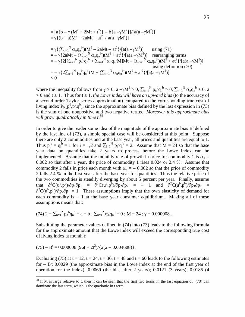
25
= [a{b (M2 + 2Mt + t
2)} b{a M
2}]/[a(a M
2)]
= {(b a)M2 2aMt at
2}/[a(a M
2)]
= {(n=1N nqn
b )tM
2 2aMt at
2}/[a(a M
2)] using (71)
= {2aMt (n=1N nqn
b )tM
2 + at
2}/[a(a M
2)] rearranging terms
= {2[n=1N pn
bqn
b + n=1
N nqn
bM]Mt (n=1
N nqn
b )tM
2 + at
2}/[a(a M
2)]
using definition (70)
= {2n=1N pn
bqn
b tM + (n=1
N nqn
b )tM
2 + at
2}/[a(a M
2)]
< 0
where the inequality follows from > 0, a M2 > 0, n=1
N pn
bqn
b > 0, n=1
N nqn
b 0, a
> 0 and t 1. Thus for t 1, the Lowe index will have an upward bias (to the accuracy of
a second order Taylor series approximation) compared to the corresponding true cost of
living index PK(p0,p
t,q
b), since the approximate bias defined by the last expression in (73)
is the sum of one nonpositive and two negative terms. Moreover this approximate bias
will grow quadratically in time t.38
In order to give the reader some idea of the magnitude of the approximate bias Bt defined
by the last line of (73), a simple special case will be considered at this point. Suppose
there are only 2 commodities and at the base year, all prices and quantities are equal to 1.
Thus pib = qi
b = 1 for i = 1,2 and i=1
N pi
bqi
b = 2. Assume that M = 24 so that the base
year data on quantities take 2 years to process before the Lowe index can be
implemented. Assume that the monthly rate of growth in price for commodity 1 is 1 =
0.002 so that after 1 year, the price of commodity 1 rises 0.024 or 2.4 %. Assume that
commodity 2 falls in price each month with 2 = 0.002 so that the price of commodity
2 falls 2.4 % in the first year after the base year for quantities. Thus the relative price of
the two commodities is steadily diverging by about 5 percent per year. Finally, assume
that 2C(u
b,p
b)/p1p1 =
2C(u
b,p
b)/p2p2 = 1 and
2C(u
b,p
b)/p1p2 =
2C(u
b,p
b)/p2p1 = 1. These assumptions imply that the own elasticity of demand for
each commodity is 1 at the base year consumer equilibrium. Making all of these
assumptions means that:
(74) 2 = n=12 pn
bqn
b = a = b ; n=1
2 nqn
b = 0 ; M = 24 ; = 0.000008 .
Substituting the parameter values defined in (74) into (73) leads to the following formula
for the approximate amount that the Lowe index will exceed the corresponding true cost
of living index at month t:
(75) Bt = 0.000008 (96t + 2t
2)/{2(2 0.004608)}.
Evaluating (75) at t = 12, t = 24, t = 36, t = 48 and t = 60 leads to the following estimates
for Bt: 0.0029 (the approximate bias in the Lowe index at the end of the first year of
operation for the index); 0.0069 (the bias after 2 years); 0.0121 (3 years); 0.0185 (4
38
If M is large relative to t, then it can be seen that the first two terms in the last equation of (73) can
dominate the last term, which is the quadratic in t term.

26
years); 0.0260 (5 years). Thus at the end of the first year of the operation of the Lowe
index, it will only be above the corresponding true cost of living index by approximately
a third of a percentage point but by the end of the fifth year of operation, it will exceed
the corresponding cost of living index by about 2.6 percentage points, which is no longer
a negligible amount.39
The numerical results in the previous paragraph are only indicative of the approximate
magnitude of the difference between a cost of living index and the corresponding Lowe
index. The important point to note is that to the accuracy of a second order
approximation, the Lowe index will generally exceed its cost of living counterpart.
However, the results also indicate that this difference can be reduced to a negligible
amount if:
the lag in obtaining the base year quantity weights is minimized and
the base year is changed as frequently as possible.
It also should be noted that the numerical results depend on the assumption that long run
trends in prices exist, which may not be true,40
and on elasticity assumptions that may not
be justified.41
Thus statistical agencies should prepare their own carefully constructed
estimates of the differences between a Lowe index and a cost of living index in the light
of their own particular circumstances.
References
Baldwin, A. (1990), “Seasonal Baskets in Consumer Price Indexes”, Journal of Official
Statistics 6:3, 251-273.
Balk, B.M. (1980), “A Method for Constructing Price Indices for Seasonal
Commodities”, The Journal of the Royal Statistical Society Series A 143, 68-75.
Bean, L. H. and O. C. Stine (1924), “Four Types of Index Numbers of Farm Prices”,
Journal of the American Statistical Association 19, 30-35.
Bortkiewicz, L.v. (1923), “Zweck und Struktur einer Preisindexzahl”, Nordisk Statistisk
Tidsskrift 2, 369-408.
Carruthers, A. G., D. J. Sellwood and P. W. Ward (1980), “Recent Developments in the
Retail Prices Index”, The Statistician 29, 1-32.
39
Note that the relatively large magnitude of M compared to t leads to a bias that grows approximately
linearly with t rather than quadratically. 40
For mathematical convenience, the trends in prices were assumed to be linear rather than the more
natural assumption of geometric trends in prices. 41
Another key assumption that was used to derive the numerical results is the magnitude of the divergent
trends in prices. If the price divergence vector is doubled to 1 = 0.004 and 2 = 0.004, then the
parameter quadruples and the approximate bias will also quadruple.

27
Dalén, J. (1992), “Computing Elementary Aggregates in the Swedish Consumer Price
Index,” Journal of Official Statistics 8, 129-147.
Diewert, W.E. (1992), “Exact and Superlative Welfare Change Indicators”, Economic
Inquiry 30, 565-582.
Diewert, W.E. (1993), “Duality Approaches To Microeconomic Theory”, pp. 105-175 in
Essays in Index Number Theory, Volume 1, Contributions to Economic Analysis
217, W.E. Diewert and A.O. Nakamura (eds.), Amsterdam: North-Holland.
Diewert, W. E. (1995), “Axiomatic and Economic Approaches to Elementary Price
Indexes”, Discussion Paper No. 95-01, Department of Economics, University of
British Columbia, Vancouver, Canada.
Diewert, W.E. (1998), “Index Number Issues in the Consumer Price Index”, The Journal
of Economic Perspectives 12:1, 47-58.
Diewert, W.E. (2002), “Harmonized Indexes of Consumer Prices: Their Conceptual
Foundations”, Swiss Journal of Economics and Statistics 138, 547-637.
Drechsler, L. (1973), “Weighting of Index Numbers in Multilateral International
Comparisons”, Review of Income and Wealth 19, 17-34.
Fisher, I. (1921), “The Best Form of Index Number”, Journal of the American Statistical
Association 17, 533-537.
Fisher, I. (1922), The Making of Index Numbers, Houghton-Mifflin, Boston.
Hausman, J. (2002), “Sources of Bias and Solutions to Bias in the CPI”, NBER Working
Paper 9298, Cambridge, MA: National Bureau of Economic Research.
Hicks, J.R. (1941-42), “Consumers’ Surplus and Index Numbers”, The Review of
Economic Studies 9, 126-137.
Hicks, J.R. (1946), Value and Capital, Second Edition, Oxford: Clarendon Press.
Hill, T. P. (1996), Inflation Accounting: A Manual on National Accounting under
Conditions of High Inflation, Paris: OECD.
Hill, T. P. (1998), “The Measurement of Inflation and Changes in the Cost of Living”,
Statistical Journal of the United Nations ECE 15, 37-51.
Konüs, A.A. (1924), “The Problem of the True Index of the Cost of Living”, translated in
Econometrica 7, (1939), 10-29.

28
Lowe, J. (1823), The Present State of England in Regard to Agriculture, Trade and
Finance, second edition, London: Longman, Hurst, Rees, Orme and Brown.
Okamoto, M. (2001), “Mid-Year Basket Index as a Practical Approximation to a
Superlative Index”, Paper presented at the Sixth Meeting of the International
Working Group on Price Indices, Canberra, April 2-6, 2001.
Schultz, B. (1999), “Effects of Using Various Macro-Index Formulae in Longitudinal
Price and Comparisons: Empirical Studies”, pp. 236-249 in Proceedings of the
Fourth Meeting of the International Working Group on Price Indices, W. Lane
(ed.), Bureau of Labor Statistics, U.S. Department of Labor, Washington D.C.
Schultze, C.L. and C. Mackie (eds.) (2002), At What Price? Conceptualizing and
Measuring Cost-of Living and Price Indices, Washington DC: National Academy
Press.
Triplett, J. E. (1981), “Reconciling the CPI and the PCE Deflator”, Monthly Labor
Review (September), 3-15.
Walsh, C. M. (1901), The Measurement of General Exchange Value, New York:
Macmillan and Co.
Walsh, C. M. (1921a), The Problem of Estimation, London: P.S. King & Son.
Walsh, C. M. (1921b), “Discussion”, Journal of the American Statistical Association 17,
537-544.
Walsh, C. M. (1932), “Index Numbers”, pp. 652-658 in Encyclopedia of the Social
Sciences, Volume 7, E. R. A. Seligman (editor in chief), New York : The
Macmillan Co.
Young, A. (1812), An Inquiry into the Progressive Value of Money in England as Marked
by the Price of Agricultural Products, London.


