Inequality Measures, Equivalence Scales and Adjustment for Household
Size and Composition
Trinity Economic Paper SeriesTechnical Paper No. 98 / 8
JEL Classification: D31 & D63
Paolo FiginiDept. of Economics
Trinity CollegeDublin 2, Ireland.
e-mail: [email protected]
AbstractTotal household income inequality can be very different from inequalitymeasured at the income per-capita level but only in recent years has the patternof this divergence been investigated. In this paper, results from Coulter et al.(1992) using a one-parameter equivalence scale are updated using data forIreland, Italy, the UK and the US. A class of two-parameter equivalence scales,representing relative weights for adults and children, is then analysed. Resultsare shown to depend on the distribution of household size and compositionamong deciles of the population. Inequality generally increases with children'sweight and decreases with adults' weight. OECD and other two-parameterequivalence scales empirically used show similar results to the one-parameterequivalence scale with elasticity around 0.5.
AcknowledgementsThis work has been supported by the grant "Borsa di Studio per ilPerfezionamento degli Studi all'Estero, Area Scienze Economico-Statistiche"from University of Pavia. Thanks to Francis O'Toole and Brian Nolan for theiruseful comments. The opinions expressed in this work are the sole responsibilityof the author and do not necessarily reflect those of the Department ofEconomics, Trinity College or of its members.
2
Studies of income distribution are heavily affected by the different
procedures that researchers can choose to measure inequality. One of the major
issues involved here is to assess the direction and the extent of the change in
inequality when different adjustments for household size and composition are
allowed.1 Until a few years ago, the relevant unit in inequality studies was
chosen between total household income (H), household per-capita income (Y)
and individual income. While individual income is the simplest unit of analysis, a
better alternative is to consider H, as the household is the locus of decisions on
income getting and income spending of individual members. An even better
solution is considered Y, in which total household income is shared equally
among the household members. Y was the preferred unit taken into
consideration until a more precise welfare analysis has been brought about in
recent years.
In fact, the analysis of Y rules out the possibility of different economies of
scale in households of different size: the underlying assumption of the household
per-capita income analysis is that the well-being of an individual sharing
£20,000 in a two-person household is the same as the well-being of an individual
sharing £40,000 in a four-person household. It seems more reasonable to
postulate the existence of positive economies of scale within the household;
hence, a consistent measure of individual well-being W can be written as in
equation (1):
W = H / Sε (1)
where H is the sum of individual incomes in the household (total household
income), S is household size and ε is a parameter representing economies of
1 Other issues refer to i) the modification of extreme incomes (the procedure is known as bottom and toprecoding); ii) the comparison across countries of definitions such as gross income, disposable income orhousehold; iii) the indices used to assess inequality (indices are neither ordinally nor cardinally equivalent).On this last point, see Cowell (1995). See also Champernowne (1974), Figini (1997), Bigsten (1991) and

3
scale within the household. ε ranges from 0 (perfect economies of scale) to 1
(absence of economies of scale). Therefore, household income H (ε = 0) and
household income per capita Y (ε = 1) are the two extreme cases of a welfare
analysis in which the elasticity of scale ε plays a fundamental role.2
Buhmann et al. (1988) find that all the equivalence scales empirically used
can be approximated by a single parameter scale as (1) and in recent years one-
parameter scales have been directly used (Atkinson et al., 1995 measure
inequality in OECD countries setting ε = 0.5). This evolution raises a few
questions about the "best" value for ε to be used and about the pattern of
inequality change when the value of ε varies. While the former problem invokes
thinking about welfare assumptions and economies of scale within households,
the latter issue has been tackled theoretically and empirically by Coulter et al.
(1992): increasing the value of ε from 0 to 1, inequality first decreases and then
increases, thus depicting a U-shape. These general findings are re-assessed in
the present paper.
Yet, equation (1) is a simplification of a more general formula in which
other household characteristics such as composition, location and age might be
considered. This approach in adjusting for household characteristics can be
represented in (2):
( )W
H
N N Nk k
=+ + +α α α ε
1 1 2 2 ...(2)
where Ni is the size of each type k of components of the household (elderly
people, adults, children…), αι is the relative weight given to them and ε
Sundrum (1990). On the technical aspects of the management of household surveys an excellent overview isprovided in Atkinson et al. (1995).2 Actually, household income inequality is not technically equal to equation 1 with a parameter ε = 0 becauseof the different weighting procedure applied to the sample of data: in the former case we weight according tothe number of households, in the latter to the number of individuals.

4
represents the economies of scale within the household. A particular sub-class of
this formula will be analysed throughout the paper.
The rest of this paper is organised as follows: in the next section the
Luxembourg Income Study (LIS) database, used in this work, is presented. In
Section II, a comparison of inequality considering H and Y inequality, following
Sundrum's analysis (Sundrum, 1990) is outlined. Section III follows the
procedure of Coulter et al. (1992) comparing inequality using equation (1) in
four different countries: Ireland, Italy, UK and US. In Section IV, a particular
subclass of formula (2) is considered: a two-parameter equivalence scale, which
distinguishes between the household head, other adults and children in the
household. A weight of 1 for the household head and weights α1 and α2 ranging
between 0 and 1 for other adults (N1) and children (N2) in the household are
respectively used (equation 3).3
WH
=1 + N + N1 1 2 2α α
. (3)
Section IV also provides a comparison between the different scales used
while Section V concludes.
Section I: The data
Since the Luxembourg Income Study (LIS) project was founded in 1983,
a huge step towards a better understanding of inequality and its measurement has
been made. The project has four main goals: i) to create a database containing
social and economic data collected in household surveys from different
countries; ii) to provide a method allowing researchers to use the data under
restrictions required by the countries providing the data; iii) to create a system to
3 OECD scale is a particular case of equation (3), in which α1 = 0.7 and α2 = 0.5. Other scales often used,attach values of 0.6 or 0.5 to α1 and 0.4 or 0.3 to α2.

5
allow remote access and to elaborate data using computer networking and iv) to
promote comparative studies on income aggregates. At this stage the LIS
database includes about 70 observations for 25 countries, covering the period
from 1967 to 1995. For almost each survey there are three different files, the
first with data at the household level (allowing sometimes a disaggregation also
among multi-family households), the second at the individual level and the third
at the child level. One of the main issues in setting up such a database is to
elaborate data from single surveys transforming variables and re-weighting
single cases so as to allow a satisfactory international comparison. Of course,
perfect comparability will never be reached but, at this stage, the LIS database
allows a good degree of comparability among countries.4
Section II: Household Income and Household Per-capita Income Inequality
How much does inequality change moving from household income (H) to
household per-capita income (Y) inequality? Is the change similar for all the
indices? Is the change similar for all the countries?
The problem can be represented in the following way: household per-
capita income is the ratio of household income over household size (S).
Y = H / S. (4)
Considering logarithmic values and the coefficient of variation (CV) as a
measure of inequality, Sundrum (1990) shows that CVY < CVH if:
22
2ρ ρCV CV CVCV
CVH S S
S
H> > or if (5)
4 Technically, the preliminary stage of the research is to set up some "jobs" (SPSS commands) which are sentvia e-mail to the server address in the LIS headquarters in Luxembourg. These jobs are automatically executedand the output is sent back to the original e-mail address in a few minutes. A complete documentation withdescription, frequencies and labels for each variable of the database is also available online(http://lissy.ceps.lu/) to allow researchers to overcome problems of definition and transformation that theirown work can require. Technical assistance is always available from LIS staff.

6
where ρ is the coefficient of correlation between household size and household
income. Since CVS is usually smaller than CVH, the right-hand side of equation
(5) is sufficiently small compared to ρ if there is strong positive correlation
between size and total household income (as there is in household data).5
Therefore, in the generality of cases, Y inequality would be lower than H
inequality. LIS database highlights this decrease in inequality moving from H to
Y, as Table 1 shows. The 22 countries for which information on inequality in
the period 1987-1992 is available are listed. For each country, three different
measures of inequality (Gini, Theil and Atkinson with a sensitivity of 0.5) are
computed. Table 1 shows that inequality generally decreases moving from H to
Y. The only cases for which inequality increases are Israel, Italy, Poland and US
(only for Gini and Theil indices).
Section III: Bringing in Economies of Scale within the Household
The procedure illustrated in the previous section is a necessary step to
avoid distortions caused by the fact that rich households have a different size
compared to poor households. Accordingly, two new elements of bias have been
introduced into the analysis: i) the implicit assumption of no intra-household
inequality: H is postulated to be evenly distributed among the components of the
household. This is not always true, particularly in the case of multi-family
households, but for the rest of the paper we will always rely on this hypothesis.
ii) The assumption of not having economies of scale within the household. If two
households, one composed of two individuals with a total income of £20,000
and another one of four components and £40,000 are considered equivalent, as
5 The average household size of the bottom decile of the distribution of total household income is the lowestwhile for the top decile it is the highest for every country in the LIS database. The number of childrenincreases until the 3rd-7th decile and then decreases and, as a result, also the number of economically activepersons (computed as the number of household components minus children) increases with total household

7
equation (4) assumes, the possibility of having intra-household economies of
scale is ruled out.
This latter assumption is now relaxed and households are adjusted in
order to catch positive economies of scale as size increases. The Buhmann's
scale (Buhmann et al., 1988), represented in equation 1, allows this possibility.
Coulter et al. (1992), explain the theoretical relationship between equivalence
scales and inequality: the well-being Wi of an individual is a function of four
different variables, total household income (H), household size (S), elasticity of
scale (ε) and household characteristics (η):
Wi = Y(Hi, Si, ει, ηι). (6)
The well-being reduces to (4) if household characteristics (such as
location, age, health) are normalised and the elasticity of scale is set equal to 1.
In this section the analysis is broadened by allowing the parameter
ε, representing the intensity of economies of scale, to vary according to the
Buhmann's scale. When ε is equal to 0, W reduces to H (perfect economies of
scale are assumed); when ε is equal to 1, W reduces to Y as in (4) (economies of
scale are ruled out and the well being of each individual is simply equal to
household per-capita income). Neither of these two cases are realistic because in
each household there are some relatively fixed expenditures that are shared
among its components (rent, bills) and the scale of the sharing is a function of
the household size. In other words, if there are economies of scale, an individual
sharing £20,000 within a two-person household is worse off than an individual
who shares £40,000 in a four-person household.
Buhmann et al. (1988) and Coulter et al. (1992) demonstrate that the
movement between household income and household per-capita income
income. Data for all the countries are available from the author. Data for Ireland, Italy, UK and US arepublished in Table 5.

8
inequality is not linear (as it could be infered from the previous section) but
involves a U-shape with respect to ε. Inequality first decreases moving from ε =
0 to a higher value and, from a certain stage up to 1, inequality increases. When
households are ranked according to their total income, rich households are the
largest ones. Therefore, when income is adjusted via the parameter ε, the
denominator in equation (1) increases respectively more than the numerator, thus
having an equalising effect on the distribution. But, for high values of ε, the re-
ranking process acts to counter-balance this change in inequality: by increasing
ε, the possibility of a re-ranking of units in the distribution augments. The total
effect on income inequality would depend on the strenght of the two effects. For
low values of ε, the re-ranking effect is not strong enough to reverse the
equalising effect but, for higher ε, the re-ranking will be strong enough to lead to
an increase in inequality. This process can be understood by looking at the
example outlined in Table 2.
Using variance as a measure of inequality, the introduction of the
parameter ε can be represented as follows:
VAR (w) = VAR (h) + VAR (sε) - 2ρε (VAR (h) VAR (s))0.5. (7)
An increase in ε widens the gap between H and W inequality. But above a
threshold level, the rise in ε implies a more likely re-ranking of the households
causing an overall decrease in the gap. The result is a composite effect depicted
by a U-pattern of inequality.
The above model has been tested by Cowell et al. (1992) on different
indices of the General Entropy Measures family (GEM), (including Theil,
Atkinson and Coefficient of Variation) and on the Gini index: data from the UK
confirmed the U-shape in inequality with respect to ε. They also find a different
skewness of the U curve for different indices: keeping everything else constant,
indices more sensitive to inequality among high-incomes (such as the Coefficient
9
of Variation) show a U curve skewed to the left, more similar to a J-shape.
Indices more sensitive to inequality among low-incomes (as Atkinson) show a U
curve more skewed to the right, more similar to an inverted J-curve (for the
explanation, see Coulter et al., 1992, p. 1073).
In this paper, LIS data for the UK 1991, the US 1991, Ireland 1987 and
Italy 1991 are used. For each country Gini, CV, Theil and Atkinson(0.5) indices
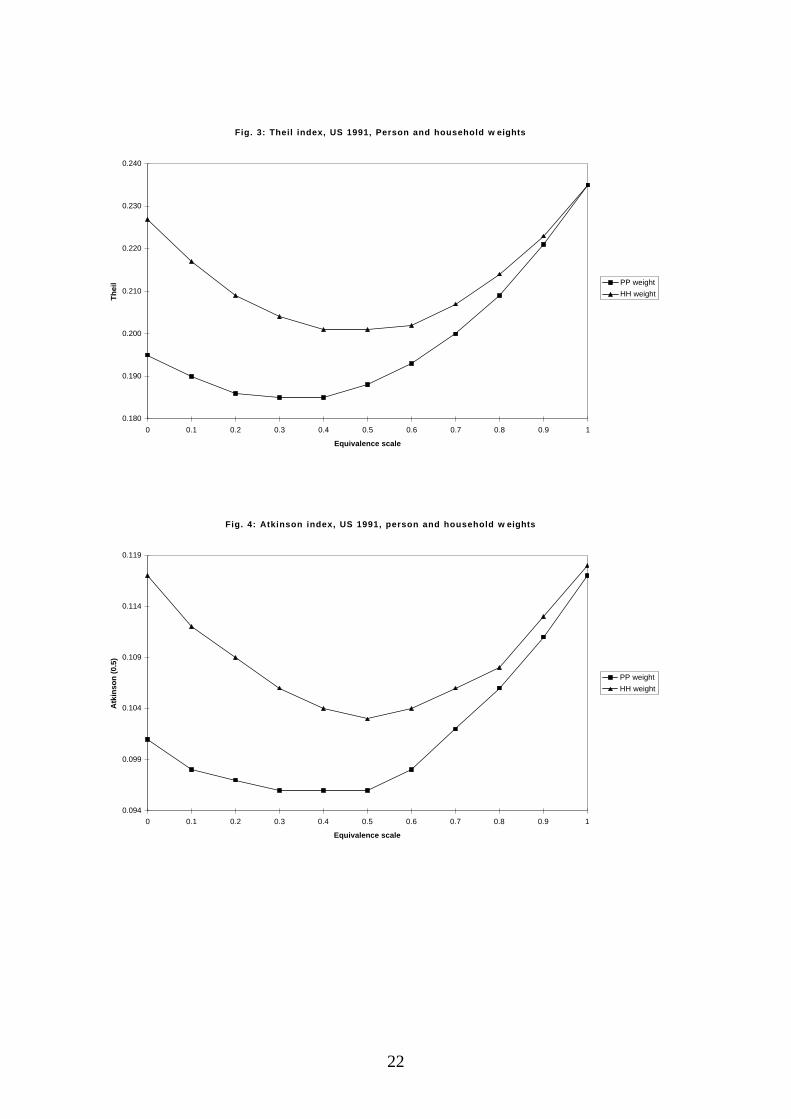
are computed for both person and household weighting.6 The main results of the
analysis are listed as follows and the patterns of inequality change are recalled in
Figures 1 and 2 (UK 1991), 3 and 4 (US 1991), 5 and 6 (Ireland 1987) and 7
and 8 (Italy 1991).
i) The U shape holds for all the countries and all the indices: inequality is
a non-linear function of ε.
ii) Contrary to the remark of Coulter et al. (Coulter et al., 1992, note 12,
p.1077) the choice of whether to weight according to the number of individuals
(PP curves in the figures) or households (HH curves in the figures) affects the
robustness of the results. Coulter et al. use household weights, finding that the
McClements equivalence scale used by the British Institute for Fiscal Studies (ε
≅ 0.6) actually minimises the extent of inequality. Using person weights, which
seem more appropriate in measuring individual well-being, the minimum of
inequality is generally reached at a lower value of ε. For this reason, the U-curve
depicted using person weights becomes more skewed to the left than the curve
drawn using household weights: the J-shape becomes more evident.
iii) The difference between PP and HH curves is not constant. For some
countries, namely the UK, the US and Ireland, the difference between PP and
6 To have results that are significant for the whole population, single cases from the sample have to beweighted. When H income (ε = 0) is measured, it seems appropriate to weight according to the number ofhouseholds (HH). With other values of the parameter, since individual well-being, is analysed, it seems moreappropriate to weight according to the number of individuals (PP). Here both possibilities are considered.
10
HH is minimised considering per-capita income (ε = 1) but this is not the only
possibility. For Italy the gap lowers until the point of minimum inequality (ε =
0.5) and then it goes up again.
iv) The values of ε for which inequality is minimised are shown in Table
3. Minima for PP are 1-2 tenth of ε lower than HH minima. Gini has the highest
minimum (ε is around 0.5/0.6 for HH) together with Atkinson. Theil is
minimised for ε around 0.4/0.5 and CV is minimised for ε around 0.4, thus
confirming the theoretical discussion by Coulter et al.: patterns for those indices
which are more sensitive to high income inequality are more skewed to the left
than indices which are more sensitive to low income inequality. For PP weights,
the minimum moves down to ε around 0.3 for CV and ε around 0.5 for Atkinson
and Gini.
v) The shape of the curves also depends on the country, with the US and
Italy being more skewed to the left than the UK and Ireland. Countries with a
higher inequality in household size distribution (UK and Ireland) are more likely
to have a U-shape skewed to the right while countries with lower inequality in
household size distribution (U.S. and Italy) seem to have a U-shape more
skewed to the left (see Table 5).
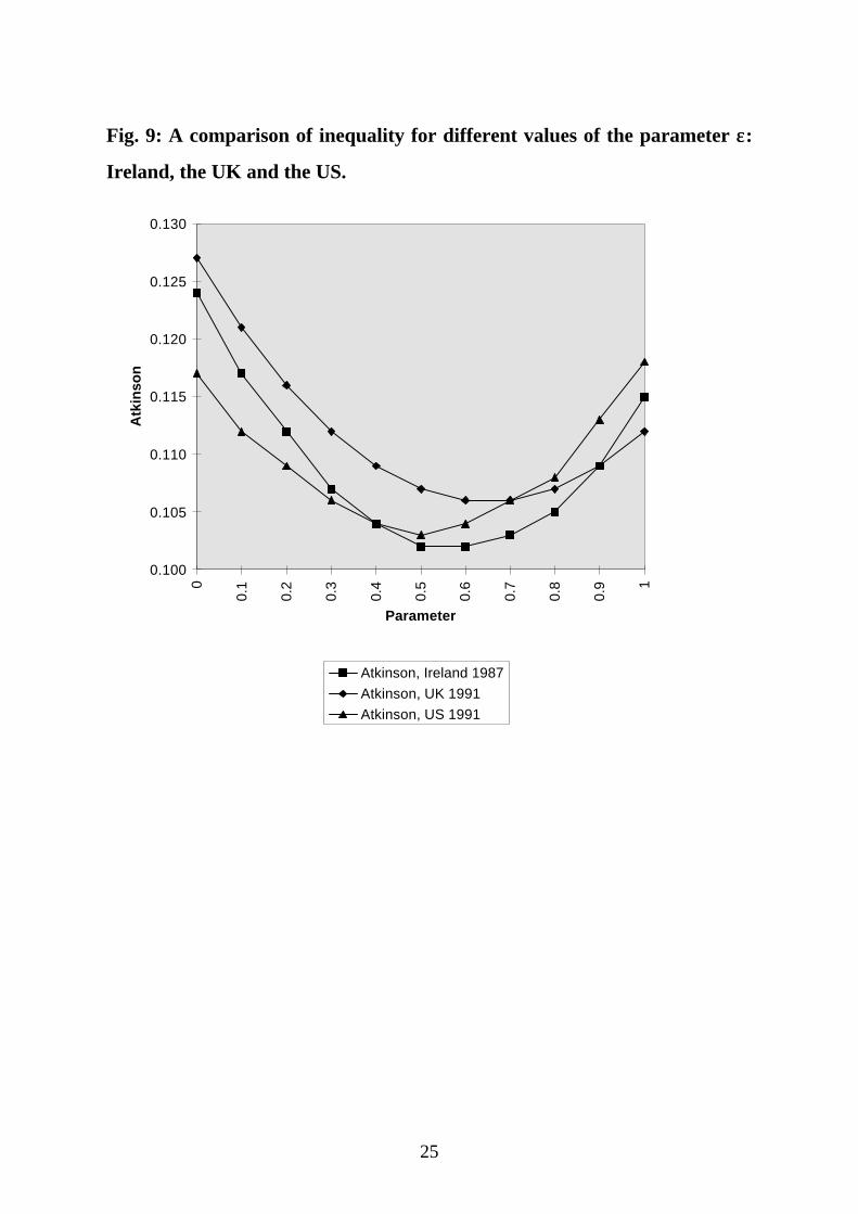
In conclusion, the use of a particular value of elasticity is fundamental in
assessing not only the absolute level of inequality and its change, but also the
ranking between countries. In fact, when the extent of inequality is similar, as it
is in the case of Ireland, the UK and the US, the ranking can be affected. The
ranking of these three countries, given the most usual assumptions (person
weighting and ε = 0.5) is shown, according to the Gini coefficient, in the second
column of Table 4. But using different assumptions (household weighting and ε
= 1), as in the third column of the same table, the ranking changes. The same
picture, using the Atkinson index and person weighting, is represented in Figure

11
9. The UK starts as the most unequal country for ε = 0 and becomes the most
equal for ε = 1.
Section IV: An Analysis with a Two-Parameter Equivalence Scale
A more precise way to adjust for household characteristics is to measure
individual welfare not only with respect to income and size, but also with respect
to the number of earners, children and elderly people in the household, as in
equation (2). An example of such an equivalence scale is the OECD scale (8):
W = H / (1 + 0.7(Nα-1) + 0.5Nc) (8)
where Nα and Nc are the number of adults and children respectively and a weight
of 1 is attached to the household head. Using the same procedure followed for
the analysis of one-parameter equivalence scale, the fundamental question that
will be tackled in this section is: how do measures of inequality change when
parameters α1 and α2 in equation 2 vary between 0 and 1?
Considering the variance as a measure of inequality, and the variables in
logarithmic terms, we have that:
VAR(w) = VAR(h) + VAR log(1+a1S1+a2S2) - 2COV(h, log(1+a1S1+a2S2)) (9)
with the chage in VAR(w) depending on the distribution of adults and children
and on their correlation with household income. To be more precise, the class of
Generalised Entropy Measures (I) is considered:7
IN
W
Wi
i=−
−∑
1
11
θ θ
θ
( )(10)
7 When θ = 1, I is equivalent to the Theil index; when θ = 2 an index cardinally equivalent to the Herfindalindex is obtained, when θ = 3 the index is ordinally equivalent to the Coefficient of Variation and when θ = 1- φ, I is ordinally equivalent to the class of Atkinson indices with parameter φ. See Cowell (1995) and Figini(1998).
12
where θ is a parameter determining the aversion to inequality, N is the number
of observations, Wi is the well being of the individual-i and W is the average of
the measure. Wi is calculated according to (11):
WH
S Si
ii i
=+ +1 1 1 2 2α α
(11)
where Hi is total household income, S1 is the number of adults in the household
minus the head, S2 is the number of children in the household, the weight of the
household head is set equal to 1, and α1 and α2 are the weights of, respectively,
other adults and children.
The differentiation of GEM with respect to changes in α1 is shown in
(12). A similar formula holds for changes in α2, the only difference being the
substitution of S1i and S1
j with S2i and S2
j in the numerator of M.
( )
∂∂α θ
θI
N
W
WMi
i1
11
1=
−
∑−
(12)
where M is:
( )M
WS W
S S
W
N
Y S
S S
W
ii
i ii j
j
j jj
=+ +
−+ +
∑1
1 1 2 2
1
1 1 2 2
2
2
1 1α α α α. (13)
This formula can be read in this way. The change in inequality depends on
θ and on the sign of M which, in turn, depends on the values of S1 and S2 in each
household. Theoretically any sign can result and empirically this would depend
on the type of distribution of adults and children among households. Table 5
shows that the number of adults generally increases along the distribution of
total household income. Given a certain weight α2, an increase in the weight
given to the number of adults raises the denominator of equation (11), thus
implying an equalising effect. Table 5 also shows that the distribution of children
13
is more heterogeneous. In the four countries under consideration, the number of
children increases up to the 3rd decile (Ireland and Italy), to the 5th (US) and to
the 7th (UK), declining thereafter. Given α1, an increase in the weight given to
children has instead a disequalising effect because rich households have,
generally, less children. The total effect, increasing at the same time α1 and α2,
is less clear and depends also on the re-ranking effect, the absolute values of S1
and S2 and the value of parameter θ in GEM.
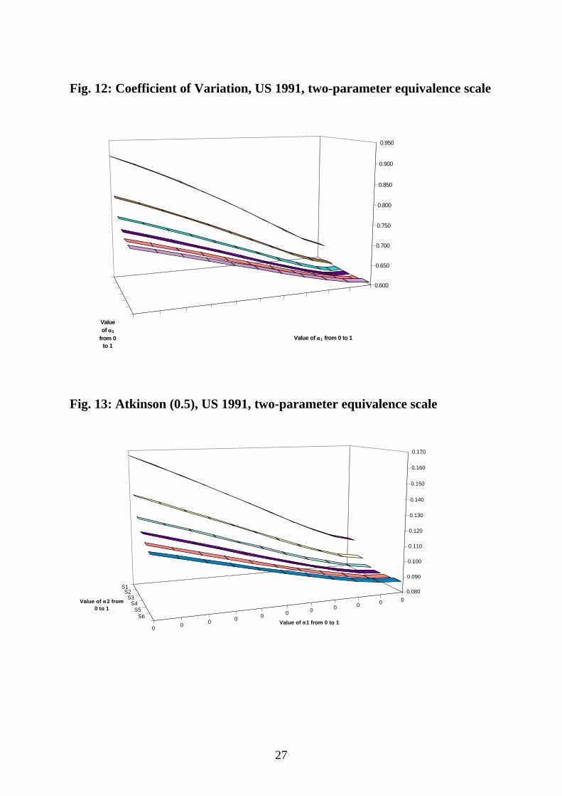
Empirically, the complexity of the situation and the possibility of
contrasting results is fortunately reduced. Given the similar pattern in adults and
children distributions among countries, a few stylised facts can be highlighted
(see also figures from 10 to 13).
i) When α1 is held fixed, inequality increases with α2; for high values of
α1, however, a J-shape appears with inequality decreasing at low values of α2.
ii) When α2 is held fixed, inequality decreases with increases in α1; for
low values of α2, however, an inverted J-shape appears with inequality
increasing at high values of α1.
iii) When the two weights vary together, the overall trend is depicted by
an inclined surface with highest inequality for low values of α1 and high values
of α2 and lowest inequality for high values of α1 and low values of α2.
Increasing both weights together we obtain a very slight U shape. Inequality is
more sensitive to changes in children's weights than to changes in adults'
weights.
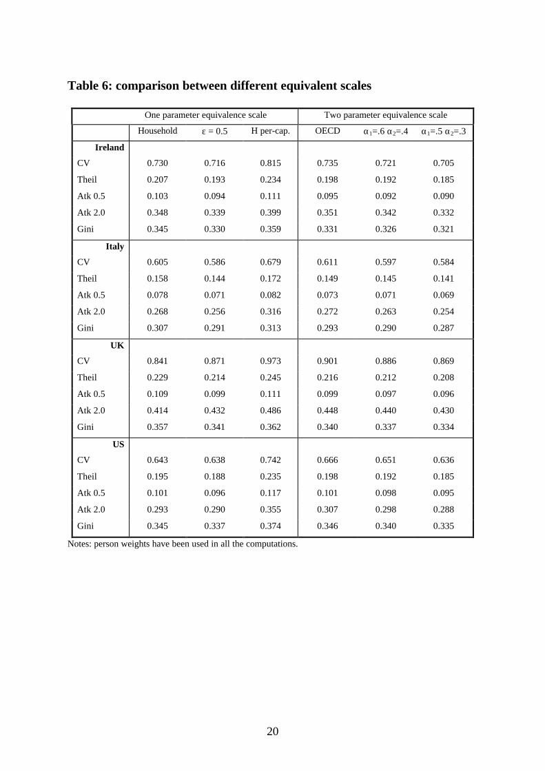
iv) Particular scales have remarkable importance: the OECD scale (α1 =
0.7 and α2 = 0.5) and other two scales in which weights are α1 = 0.6 and α2 =
0.4 and α1 = 0.5 and α2 = 0.3 respectively. Among two-parameter scales, their
values are in the middle of the range, with OECD showing the highest value of
inequality of the three. Compared to one-parameter scales, Table 6 shows that
14
they are very close to the value that we would get using (1) with ε around 0.5-
0.6.
Section V: Concluding Remarks about Inequality Comparisons
The extent of inequality is heavily dependent on the type of adjustment for
household size and composition and on the value of the parameter used to
describe economies of scale within the household. Few remarks can be outlined.
i) Among one-parameter scales, each country and each index has a
peculiar way of reacting to the choice of the elasticity of scale. Inequality has a
U-shape with respect to the value of ε, but the skewness of the curve, the
difference between two alternative weighting procedures (person and household
weights) and the value of ε which minimises inequality vary considerably.
ii) These multiple variations affect quite heavily the robustness of
inequality measurement. When one single country is analysed, the range of
values that the index can have might be larger than changes in "real" inequality:
in Table 4, between the highest and the lowest value of Gini for Ireland 1987
there is a difference of 12% which is larger than any "real" change of inequality
experienced by that country over time. More important is the fact that the
ranking of countries in the "inequality league" can be affected by the parameter
chosen.
iii) Using two-parameter equivalence scales, an increase in the weight of
the adults decreases inequality while an increase in the weight of children
increases inequality very heavily. For extreme values of the weights (high α1 and
low α2) the change in the other weight can provoke a J or an inverted J-shape.
These results are not a "law" but stylised facts due to the particular pattern of
distribution of adults and children among households ranked with respect to
15
income. When the two weights are increased together both a J-shape and a linear
increase in the measure of inequality can appear.
iv) The two-parameter scales empirically used are very close to the one-
parameter scale with a value of ε around 0.5-0.6. OECD scale slightly over-
measures inequality compared to one-parameter with ε = 0.5.
v) Also for two-parameter scales, the robustness of the results depends on
the index used, the country under examination and the distribution of children
and adults within each household. In theory a broad spectrum of heterogeneous
results might appear.
vi) Empirically, inequality as measured using the most common
equivalence scales does not change considerably. This is not due to an intrinsic
robustness of results but is the consequence of the fact that equivalence scales
empirically used have very similar underlying assumptions. On the other hand,
the use of odd scales (e.g., α1 = 0 and α2 = 1) can produce very particular
results. This general conclusion is twinned to another similar conclusion
regarding the choice of the index. The most common indices of inequality
produce very similar results because they have very similar aversions to
inequality. Particular aversions to inequality (as for the Coefficient of variation
or for the Atkinson (ε=2) index) produce peculiar measures of inequality.8
vii) While we need to be aware of the sensitivity of results to changes in
the equivalence scale, in empirical studies there is a tendency towards using ε =
0.5. Yet, a comparison of well-being between countries should allow ε to take
different values for each country in order to catch in a more precise way the
country's peculiarity in terms of household structure and within-household
economies of scale. As we can easily figure out, this might have disruptive
8 For a study of how inequality changes changing the indices used, see Figini (1998).

16
consequences on the way in which inequality is measured but, without any
doubt, further research is needed in this area.

17
Table 1: inequality considering different recipient units
Country Unit Gini Theil AtkinsonAUSTRALIA '89 H 0.354 0.210 0.107AUSTRALIA '89 Y 0.333 0.191 0.093BELGIUM '92 H 0.301 0.150 0.081BELGIUM '92 Y 0.251 0.108 0.057CANADA '91 H 0.339 0.192 0.097CANADA '91 Y 0.312 0.167 0.081
CZECH REPUBLIC '92 H 0.297 0.152 0.073CZECH REPUBLIC '92 Y 0.210 0.086 0.039
DENMARK '92 H 0.342 0.201 0.103DENMARK '92 Y 0.248 0.120 0.059FINLAND '91 H 0.313 0.158 0.081FINLAND '91 Y 0.256 0.114 0.054FRANCE '89 H 0.390 0.272 0.145FRANCE '89 Y 0.380 0.263 0.134
HUNGARY '91 H 0.364 0.229 0.115HUNGARY '91 Y 0.294 0.165 0.081IRELAND '87 H 0.381 0.252 0.124IRELAND '87 Y 0.359 0.234 0.111ISRAEL '92 H 0.347 0.199 0.098ISRAEL '92 Y 0.355 0.222 0.102ITALY '91 H 0.330 0.182 0.091ITALY '91 Y 0.313 0.172 0.082
NETHERLANDS '91 H 0.325 0.191 0.097NETHERLANDS '91 Y 0.316 0.187 0.091
NORWAY '91 H 0.333 0.189 0.095NORWAY '91 Y 0.253 0.114 0.055POLAND '92 H 0.323 0.177 0.086POLAND '92 Y 0.326 0.184 0.088RUSSIA '92 H 0.501 0.631 0.230RUSSIA '92 Y 0.440 0.550 0.187
SLOVAKIA '92 H 0.285 0.135 0.067SLOVAKIA '92 Y 0.202 0.074 0.035
SPAIN '90 H 0.349 0.211 0.102SPAIN '90 Y 0.326 0.194 0.091
SWEDEN '92 H 0.329 0.178 0.091SWEDEN '92 Y 0.251 0.108 0.054
SWITZERLAND '82 H 0.385 0.308 0.137SWITZERLAND '82 Y 0.361 0.274 0.117
TAIWAN '91 H 0.338 0.203 0.096TAIWAN '91 Y 0.322 0.194 0.086
UK '91 H 0.389 0.271 0.127UK '91 Y 0.362 0.245 0.111USA '91 H 0.372 0.227 0.117USA '91 Y 0.374 0.235 0.117
Notes: H = total household income; Y = household per-capita income. Household inequality measuredweighting for the number of households. In italics cases where inequality increases moving from H to Y.

18
Table 2: extent of inequality (coefficient of variation) of a sampledistribution when different adjustments for household size are made
Indiv. component Individual income when different parameters are consideredεε = 0 εε = 0.3 εε = 0.6 εε = 1
1, A 10 10 10 102, A 18 14.62 11.88 92, B 18 14.62 11.88 93, A 26 18.70 13.45 8.673, B 26 18.70 13.45 8.673, C 26 18.70 13.45 8.674, A 35 21.60 13.33 74, B 35 21.60 13.33 74, C 35 21.60 13.33 74, D 35 21.60 13.33 74, E 35 21.60 13.33 7
Mean income ofthe sample
27.181 18.485 12.796 8.092
Coeff. of Var. 0.324 0.210 0.086 0.137Notes: Income distribution adjusted for household size (person weighting). Number of households: 4. Totalhousehold income: [10, 18, 26, 35]. Household size: [1, 2, 3, 5]. Households are numbered while individualsare represented by letters. In the first column each individual is named after his/her belonging to one of thefour households. In the following columns adjusted income is computed according to the formula:
Y = Total Household Income / Household sizeε
for values of ε respectively of 0, 0.3, 0.6, 1. Inequality decreases from column 2 to 3 and to 4 because of theequalising effect due to increasing ε. Re-ranking effect, which starts in column 3 (members of household Nr. 4become poorer than members of household 3), becomes more evident in column 4. Its disequalising effectbecomes stronger in column 4 driving the overall inequality, as the coefficient of variation shows, up again.
Table 3: values of εε for which inequality is minimised for different choicesof country, index and weighting procedure
GiniHH GiniPP CVHH CVPP TheilHH TheilPP AtkHH AtkPP
Ireland 0.6 0.4/0.5 0.5 0.3 0.5/0.6 0.4/0.5 0.5/0.6 0.4/0.5Italy 0.5 0.4/0.5 0.4 0.4 0.4/0.5 0.4 0.5 0.4/0.5UK 0.6/0.7 0.4/0.5 0.4 0 0.6 0.4/0.5 0.6/0.7 0.4/0.5US 0.5 0.3/0.4 0.4 0.3 0.4/0.5 0.3/0.4 0.5 0.3/0.4/0.5

19
Table 4 - Inequality ranking using different assumptions
GiniPP, εε = 0.5 GiniHH, εε = 1UK 0.341 (1) 0.363 (3)US 0.337 (2) 0.364 (2)
Ireland 0.330 (3) 0.375 (1)Notes: in column 2, Gini is computed using person weights and ε is set equal to 0.5. In column 3, Gini iscomputed using household weights and ε is set equal to 1.
Table 5: average household size and composition in selected countries
Ireland (1987) Italy (1991) United Kingdom(1991)
United States (1991)
Deciles size adults childrn size adults childrn size adults childrn size adults childrn
1 2.83 1.74 1.09 2.61 2.02 .59 1.84 1.39 .45 2.46 1.51 .95
2 3.70 2.03 1.67 3.21 2.28 .93 2.42 1.68 .74 2.97 1.82 1.15
3 4.74 2.15 2.59 3.44 2.41 1.03 2.88 1.84 1.04 3.31 1.98 1.33
4 4.74 2.28 2.46 3.54 2.55 .99 3.14 1.97 1.17 3.33 2.09 1.24
5 4.67 2.39 2.28 3.61 2.68 .93 3.24 2.07 1.17 3.61 2.23 1.38
6 4.87 2.64 2.23 3.69 2.79 .90 3.39 2.19 1.20 3.59 2.24 1.35
7 5.15 2.83 2.32 3.75 2.89 .86 3.55 2.31 1.24 3.56 2.36 1.20
8 5.14 2.85 2.29 3.91 3.03 .88 3.42 2.40 1.02 3.66 2.46 1.20
9 5.36 3.37 1.99 4.13 3.29 .84 3.36 2.47 .89 3.80 2.61 1.19
10 5.49 3.90 1.59 4.13 3.48 .65 3.73 2.72 1.01 4.08 2.93 1.15
CV 0.175 0.249 0.227 0.126 0.165 0.162 0.186 0.189 0.246 0.132 0.182 0.102
Notes: average size, number of adults and number of children in each decile of the population. A measure ofinequality CV (coefficient of variation) for the variables is calculated in the last row.
20
Table 6: comparison between different equivalent scales
One parameter equivalence scale Two parameter equivalence scale
Household ε = 0.5 H per-cap. OECD α1=.6 α2=.4 α1=.5 α2=.3
Ireland
CV 0.730 0.716 0.815 0.735 0.721 0.705
Theil 0.207 0.193 0.234 0.198 0.192 0.185
Atk 0.5 0.103 0.094 0.111 0.095 0.092 0.090
Atk 2.0 0.348 0.339 0.399 0.351 0.342 0.332
Gini 0.345 0.330 0.359 0.331 0.326 0.321
Italy
CV 0.605 0.586 0.679 0.611 0.597 0.584
Theil 0.158 0.144 0.172 0.149 0.145 0.141
Atk 0.5 0.078 0.071 0.082 0.073 0.071 0.069
Atk 2.0 0.268 0.256 0.316 0.272 0.263 0.254
Gini 0.307 0.291 0.313 0.293 0.290 0.287
UK
CV 0.841 0.871 0.973 0.901 0.886 0.869
Theil 0.229 0.214 0.245 0.216 0.212 0.208
Atk 0.5 0.109 0.099 0.111 0.099 0.097 0.096
Atk 2.0 0.414 0.432 0.486 0.448 0.440 0.430
Gini 0.357 0.341 0.362 0.340 0.337 0.334
US
CV 0.643 0.638 0.742 0.666 0.651 0.636
Theil 0.195 0.188 0.235 0.198 0.192 0.185
Atk 0.5 0.101 0.096 0.117 0.101 0.098 0.095
Atk 2.0 0.293 0.290 0.355 0.307 0.298 0.288
Gini 0.345 0.337 0.374 0.346 0.340 0.335
Notes: person weights have been used in all the computations.

21
Fig. 1: Gini index, the UK 1991, for both person and household w eighting
0 . 3 3
0 . 3 4
0 . 3 5
0 . 3 6
0 . 3 7
0 . 3 8
0 . 3 9
0 . 4
0 0 . 1 0 . 2 0 . 3 0 . 4 0 . 5 0 . 6 0 . 7 0 . 8 0 . 9 1
Equivalence scale
Gin
i Gini, ppw eight
Gini, hhw eight
Fig. 2: Coefficient of Variation, the UK 1991, for both person and household w eighting
0 . 8 0 0
0 . 8 2 0
0 . 8 4 0
0 . 8 6 0
0 . 8 8 0
0 . 9 0 0
0 . 9 2 0
0 . 9 4 0
0 . 9 6 0
0 . 9 8 0
1 . 0 0 0
0 0 . 1 0 . 2 0 . 3 0 . 4 0 . 5 0 . 6 0 . 7 0 . 8 0 . 9 1
Equivalence scale
CV
CV, ppweight
CV, hhweight
22
Fig. 3: Theil index, US 1991, Person and household w eights
0.180
0.190
0.200
0.210
0.220
0.230
0.240
0 0.1 0.2 0.3 0.4 0.5 0.6 0.7 0.8 0.9 1
Equivalence scale
Th
eil PP weight
HH weight
Fig. 4: Atkinson index, US 1991, person and household w eights
0.094
0.099
0.104
0.109
0.114
0.119
0 0.1 0.2 0.3 0.4 0.5 0.6 0.7 0.8 0.9 1
Equivalence scale
Atk
inso
n (
0.5)
PP weight
HH weight

23
Fig. 5: Gini index, Ireland 1987, person and household w eights
0 . 3 2 0
0 . 3 3 0
0 . 3 4 0
0 . 3 5 0
0 . 3 6 0
0 . 3 7 0
0 . 3 8 0
0 . 3 9 0
0 0 . 1 0 . 2 0 . 3 0 . 4 0 . 5 0 . 6 0 . 7 0 . 8 0 . 9 1
Equivalence scale
Gin
i
Gini (HH w eight)
Gini (PP w eight)
Fig. 6: Atkinson index, Ireland 1987, person and household w eights
0 . 0 9 0
0 . 0 9 5
0 . 1 0 0
0 . 1 0 5
0 . 1 1 0
0 . 1 1 5
0 . 1 2 0
0 . 1 2 5
0 0 . 1 0 . 2 0 . 3 0 . 4 0 . 5 0 . 6 0 . 7 0 . 8 0 . 9 1
Equivalence scale
Atk
inso
n
Atk inson (HH weight)
Atkinson (PP weight)

24
Fig. 7: Coefficient of Variation, Italy 1991, person and household w eights
0 . 4 5 0
0 . 5 0 0
0 . 5 5 0
0 . 6 0 0
0 . 6 5 0
0 . 7 0 0
0 . 0 0 0 . 1 0 0 . 2 0 0 . 3 0 0 . 4 0 0 . 5 0 0 . 6 0 0 . 7 0 0 . 8 0 0 . 9 0 1 . 0 0
Equivalence scale
CV
CV, PPw eight
CV, HHweight
Fig. 8: Atkinson index, Italy 1991, person and household w eights
0 . 0 5 0
0 . 0 5 5
0 . 0 6 0
0 . 0 6 5
0 . 0 7 0
0 . 0 7 5
0 . 0 0 0 . 1 0 0 . 2 0 0 . 3 0 0 . 4 0 0 . 5 0 0 . 6 0 0 . 7 0 0 . 8 0 0 . 9 0 1 . 0 0
Equivalence scale
Atk
inso
n, 0
.5
Atk inson, ppweight
Atk inson, hhweight
25
Fig. 9: A comparison of inequality for different values of the parameter εε:
Ireland, the UK and the US.
0.100
0.105
0.110
0.115
0.120
0.125
0.130
0
0.1
0.2
0.3
0.4
0.5
0.6
0.7
0.8
0.9 1
Parameter
Atk
inso
n
Atkinson, Ireland 1987
Atkinson, UK 1991
Atkinson, US 1991

26
Fig. 10: Theil index, Ireland 1987, two-parameter equivalence scale
12345678910
11
S1
S3
S5
S7
S9
S11
0.150
0.200
0.250
0.300
0.350
0.400
0.450
0.500
Value of αα1 from 0 to 1
Value of αα2 from0 to 1
Fig. 11: Coeff. of variation, Ireland 1987, two-parameter equivalence scale
b1000000000
0
S1
S3
S5
S7
S9
S11
0.600
0.700
0.800
0.900
1.000
1.100
1.200
Value of a1 from 0 to 1
Value of a2 from0 to 1
27
Fig. 12: Coefficient of Variation, US 1991, two-parameter equivalence scale
0.600
0.650
0.700
0.750
0.800
0.850
0.900
0.950
Value of αα1 from 0 to 1
Value of αα2
from 0 to 1
Fig. 13: Atkinson (0.5), US 1991, two-parameter equivalence scale
0000000000
0
S1S2
S3S4
S5S6
0.080
0.090
0.100
0.110
0.120
0.130
0.140
0.150
0.160
0.170
Value of αα1 from 0 to 1
Value of αα2 from0 to 1

28
References
Atkinson, A.B., Rainwater, L., Smeeding T., (1995), Income Distribution in
OECD countries, Paris, OECD.
Bigsten, A., (1991), Income, Distribution and Development, London,
Heinemann.
Buhmann, B., Rainwater, L., Schmaus, G., Smeeding, T., (1988), 'Equivalence
scales, well-being, inequality and poverty: sensitivity estimates across ten
countries using the Luxembourg Income Study database', Review of Income
and Wealth, Vol. 34, No. 1, pp. 115-42.
Champernowne, D.G., (1974), 'A comparison of measures of inequality of
income distribution', The Economic Journal, Vol. 84, pp. 787-815.
Coulter, F.A.E., Cowell, F.A., Jenkins, S.P., (1992), 'Equivalence scale
relativities and the extent of inequality and poverty', The Economic
Journal, Vol. 102, pp. 1067-82.
Cowell, F.A., (1995), Measuring Inequality, London, Prentice Hall, 2nd edition.
Figini, P., (1998), 'Measuring inequality: on the correlation between indices',
Trinity Economic Papers, No. 98 / 7, Dublin, Trinity College.
Jenkins, S.P. and Cowell, F.A., (1994), 'Parametric equivalence scales and scale
relativities', The Economic Journal, Vol. 104, pp. 891-900.
Sundrum, R.M., (1990), Income Distribution in Less Developed Countries,
London, Routledge.


