
Information Asymmetry and Insider Trading*
Wei Wu†
Job Market Paper
November 2014
Abstract
I investigate the impact of information asymmetry on insider trading by exploiting a quasi-
experimental design: the brokerage closure-related terminations of analyst coverage, which
exogenously increase the information asymmetry of the affected firms. Using a difference-in-
differences approach, I find that after the terminations of analyst coverage, corporate insiders
obtain significantly higher abnormal returns and enjoy larger abnormal profits. The magnitudes
of the increase are large economically. For firms with five or fewer analysts, losing one analyst
increases insiders’ six-month abnormal returns by 16.0% for purchases, and by 10.7% for sales
(both in absolute terms). My paper highlights the role of information asymmetry as a critical
determinant of insiders’ abnormal profits, and calls for regulatory attention to corporate insiders’
transactions associated with high levels of information asymmetry.
* I am extremely grateful to my advisors Eugene Fama, Bryan Kelly, Tobias Moskowitz, and Amit Seru for their
invaluable advice and guidance. I would also like to thank Bruno Biais, Lauren Cohen, John Core, Zhiguo He,
Steven Kaplan, Ralph Koijen, Christian Leuz, Marina Niessner, Jacopo Ponticelli, Antoinette Schoar, Kelly Shue,
Douglas Skinner, Eric So, Adrien Verdelhan, and the members of the University of Chicago Booth School of
Business Fama-Miller Corporate Finance Reading Group as well as seminar participants at the University of
Chicago Booth School of Business Finance Workshop, the University of Chicago Booth School of Business Student
Brownbag, and the Massachusetts Institute of Technology Finance Lunch Workshop for their feedback and
comments. I am grateful to Bryan Kelly and Alexander Ljungqvist for sharing the closure-related coverage
termination data. I acknowledge financial support from the Deutsche Bank Doctoral Fellowship, the Katherine
Dusak Miller PhD Fellowship, the Eugene F. Fama PhD Fellowship, and the John and Serena Liew Fellowship Fund
at the Fama-Miller Center for Research in Finance, the University of Chicago Booth School of Business. All
remaining errors are my own.
† University of Chicago Booth School of Business. E-mail: [email protected]. Please check for update at
http://home.uchicago.edu/~wwu0/papers.html

1
1. Introduction
Informed traders (e.g., hedge funds and corporate insiders) in the financial market have better
information regarding the traded assets than uninformed traders (e.g., retail investors). This paper
terms the informational advantage of the informed traders over uninformed traders as
information asymmetry. Informed traders exploit information asymmetry through their
transactions. During this process, they impound their private information into asset prices and
can make the capital markets more efficient. Thus, investigating the impact of information
asymmetry on the behavior and outcome of informed trading can help researchers better
understand the price-discovery process. It can also help investors evaluate the performance of
active management, because we would like to know the returns one can earn if he or she
possesses valuable private information. On the other hand, because informed traders obtain
abnormal profits at the expense of uninformed traders, large abnormal profits of informed traders
can raise alarm regarding the fairness and integrity of the financial market, and thus discourage
capital market participation.1
Therefore, understanding the relation between information
asymmetry and insider trading is also of interest to policymakers who aim to preserve market
integrity.
The theoretical literature has made substantial progress in characterizing the trading
behavior of informed traders (e.g., Grossman and Stiglitz 1980, Kyle 1985, Copeland and Galai
1983, Spiegel and Subrahmanyam 1992, Back 1992). For example, Kyle’s seminal model
predicts a positive relation between information asymmetry and the abnormal profits of informed
traders. However, testing this relation is an empirical challenge, because information asymmetry
is time varying and, more importantly, unobservable. Previous studies have relied on proxies for
information asymmetry, such as the level of institutional ownership and the number of analysts
covering a stock, to study the correlation between information asymmetry and insider trading.
These studies (e.g., Huddart and Ke, 2007) have reported mixed results across proxies.
Moreover, for a given proxy, the results are often inconsistent across insider purchases and sales
samples. Up to now, our understanding regarding the relation between information asymmetry
and insider trading has remained limited.
A critical problem associated with the proxies for information asymmetry is the omitted
variables issue. In particular, both the proxies for information asymmetry and the outcome and
behavior of insider trading can be driven by private information regarding the prospects of the
firms. For instance, studies have used the number of analysts as a proxy for information
1 See Leland (1992) and Bhattacharya (2014) for the commonly argued pros and cons of insider trading.

2
asymmetry, because research analysts are an important information source for outsiders.
Analysts analyze, interpret, and disseminate information to capital market participants, and thus
help reduce the informational advantage of the insiders (Womack 1996, Barber et al. 2001,
Gleason and Lee 2003, Jegadeesh et al. 2004, Brown et al. 2014). However, variation in the
number of analysts, such as the termination of an existing coverage or the initiation of a new
coverage, is likely influenced by the analysts’ private information about the prospects of the
covered firm. Meanwhile, insiders can trade based on their private information about the firms’
prospects. Therefore, an OLS regression between the number of analysts and insiders’ abnormal
returns will yield biased estimates because the omitted variable, the prospects of the covered
firms, is correlated with both the proxy and insiders’ returns.
To deal with the endogeneity problem, I exploit a quasi-experimental design and use a
difference-in-differences (DiD) approach to establish a causal link between the number of
analysts and insider trading. The identification strategy I use in this paper relies on the closure-
related coverage terminations, which are reductions of analyst coverage due to the fact that 43
brokerage firms close their research departments between 2000 and 2008. Unlike typical changes
in analyst coverage, closure-related terminations are driven by the unfavorable economic
condition of the brokerage firms and are shown to be neither economically nor statistically
related to the subsequent performance of the covered stocks (Kelly and Ljungqvist 2012, Hong
and Kacperczyk 2010). Therefore, closure-related terminations of analyst coverage increase the
informational advantage of the insiders exogenously, and thus provide me with a clean
environment to identify the causal impact of coverage reduction on insider trading.
I merge the corporate insider trading data with the closure-related coverage termination
data to construct the sample in my study. I focus on corporate insiders because they are a group
of informed traders who possess firm-specific private information and are required to disclose
their transactions. Because the coverage terminations have a stronger impact on information
asymmetry in firms with lower levels of initial coverage,2 I focus on the subsample with treated
firms that have five or fewer analysts prior to the coverage reductions in most analysis of my
paper.3
2 For example, losing one analyst in a firm with three analysts prior to the coverage reductions is much more likely
to have a strong impact on firms’ information environment compared to losing one analyst in a firm with 20 analysts
prior to the coverage reductions.
3 In section 4.1, I relax this constraint and provide heterogeneity tests across the levels of the initial coverage. I show
the treatment effects are much weaker in firms with more than five analysts prior to the coverage terminations.
Except for section 4.1, all analysis in my paper is performed in the subsample with treated firms that have five or
fewer analysts prior to the coverage reductions.

3
I first examine the changes in insiders’ abnormal returns around the terminations of
analyst coverage. Consistent with the predictions of various informed-trading models (e.g.,
Grossman and Stiglitz 1980, Kyle 1985, Copeland and Galai 1983, Spiegel and Subrahmanyam
1992, Back 1992), I find insiders’ abnormal returns increase significantly after terminations of
analyst coverage. This increase takes place in both the insider purchases sample and insider sales
sample, in which the changes in stock abnormal returns exhibit opposite signs. The six-month
cumulative abnormal returns increase by 16.0% in absolute terms following the terminations of
analyst coverage in the insider purchases sample, suggesting insiders enjoy higher abnormal
returns from their purchases, whereas the six-month cumulative abnormal returns decrease by
10.7% in absolute terms following the terminations of analyst coverage in the insider sales
sample, suggesting insiders avoid more losses from their sales. These results are robust to the
inclusion of firm fixed effects (or firm × insider fixed effects), transaction-date fixed effects, and
control variables, indicating the treatment effects are not due to systematic differences in firms,
insiders, transaction dates, or control variables. The large magnitude of the treatment effects
highlights the time-varying feature of insiders’ abnormal returns and indicates information
asymmetry is a critical determinant of insiders’ abnormal returns.
To better understand the source of the treatment effects, I systematically examine the
change of insiders’ abnormal returns cumulated in different time windows. I find the majority of
the increase in insiders’ abnormal returns comes after the filing dates of their transactions. The
surprisingly slow price-discovery process suggests the public disclosure requirement of insiders’
transactions is not enough to guarantee price efficiency. Moreover, I show that a significant
portion of the increase in insiders’ abnormal returns is concentrated in narrow time windows
surrounding the release of corporate news such as earnings announcements and 8-K filings. This
finding suggests the edge insiders have over uninformed traders lies in their firm-specific private
information.
After documenting the impact of coverage reductions on insiders’ abnormal returns, I
present evidence that shows the heterogeneity in the treatment effects. The increase in insiders’
abnormal returns is more pronounced in firms with fewer analysts covering the firm,
corroborating the identification strategy by showing that insider trading responds to larger
percentage drops in analyst coverage.4 The increase in insiders’ abnormal returns is stronger in
firms with a higher percentage of insiders that exhibit opportunistic trading patterns, whose
trades are more likely driven by their private information. Moreover, the desire to diversify plays
4 I also use a specification that parametrically adjusts the treatment intensity by assuming the increase in information
asymmetry is inversely proportional to the amount of initial coverage. I run this specification in the full sample, and
the results are consistent with those in the baseline analysis.

4
a role in influencing insiders’ trading behavior. Insiders are less likely to take advantage of the
increase in information asymmetry through purchases, and are more likely to do so through sales
if the stockholdings of their own companies comprise a large portion of their wealth portfolios.
Finally, regulatory attention can shape insiders’ abnormal returns. The increase in insiders’
abnormal returns is much lower in time periods with higher intensity of legal enforcement,
suggesting insiders are concerned about litigation risks associated with their transactions.
I perform a range of robustness checks to confirm the validity of the empirical tests. First,
I study the dynamics of the treatment effects. I confirm that no pre-trends are present in either the
insider purchases sample or the insider sales sample. I also show the duration of the treatment
effects depends on the recovery pattern of the number of analysts. The increase in insiders’
abnormal returns decays six months after the coverage reductions in firms whose number of
analysts rebounds rapidly. Next, I construct portfolios consisting of insiders’ transactions and
examine their performance. Consistent with the DiD analysis at the transaction level, I find the
alphas of the insider-purchases portfolios increase significantly, whereas the alphas of the
insider-sales portfolios decrease significantly after the terminations of analyst coverage. Finally,
I confirm the treatment effects are robust to alternative measures of abnormal returns, the
inclusion of liquidity measures, and the exclusion of tiny firms and low-price transactions,
whereas they disappear in the placebo tests in which I falsely shift the termination dates or
replace the treated firms with similar control firms.
Terminations of analyst coverage also alter insiders’ trading behavior in both the
intensive and extensive margins. In particular, I find insiders’ trading volume, transaction value,
and trading probability for liquid stocks increase significantly after the terminations of analyst
coverage. These results are consistent with the price-taking models (e.g., Grossman and Stiglitz
1980), which assume insiders’ transactions have little influence on the stock prices. For illiquid
stocks, I observe no significant changes in the insiders’ trading volume, transaction value, and
trading probability in response to the increase in information asymmetry. These results are more
consistent with the imperfect-competition models (e.g., Kyle 1985, Copeland and Galai 1983,
Spiegel and Subrahmanyam 1992), which take the price impact of insider transactions into
consideration and hence predict little to no change in the expected trade size despite an increase
in information asymmetry.
To assess the economic losses that outsiders can incur when information asymmetry
increases, I estimate the change in insiders’ abnormal profits after the terminations of analyst
coverage. Conditional on holding his or her position for six months for all trades within the one-
year post-termination period, an average insider makes $87,444 more profits from purchases, and

5
avoids $896,916 more losses from sales. These changes in the insiders’ abnormal profits are
economically sizable compared to their compensation.5 In fact, they are comparable to the
abnormal profits in the illegal insider trading cases.6 Thus, my analysis calls for regulatory
attention to the corporate insiders’ transactions, especially for those associated with high levels
of information asymmetry. Despite their easy access to non-public information, corporate
insiders have not been the primary targets of legal investigations. In all cases prosecuted by the
SEC, only around 20% of defendants are employees of stocks they traded, most of which are not
those subject to the filing requirement of the SEC (Del Guercio, Odders-White, and Ready
2013). In fact, the SEC has not prosecuted any of the insiders in my data at this time. This
somewhat puzzling fact may be due to the difficulty in identifying insiders’ transactions
associated with high levels of information asymmetry. Traditional proxies for information
asymmetry, such as the bid-ask spreads, idiosyncratic volatility and the number of analysts, fail
to explain the change in insiders’ abnormal returns after exogenous terminations of analyst
coverage. A naive regulator who relies on these measures would miss the opportunity to detect
the increase in insiders’ abnormal returns documented in my study.
My identification strategy allows me to make a causal statement about the effect of
coverage reductions on insider trading. The empirical setup, however, does not directly establish
that the impact on insider trading is caused by the increase in information asymmetry. For
example, other aspects of the firms that are also influenced by coverage reductions might drive
the results. One prominent example is the risk premium of the affected firms. I provide several
pieces of evidence that argue against the risk-premium-based alternative story. Specifically,
changes in the risk premium cannot explain the bidirectional changes of the stock abnormal
returns in the insider purchases and insider sales samples, nor can they explain the concentration
of the increase in insiders’ abnormal returns surrounding the release of corporate news.
Moreover, the changes in insiders’ abnormal returns exhibit similar patterns in the portfolio
analysis in which I control for the risk exposure separately for time periods both before and after
the coverage reductions, and in specifications in which I control for liquidity measures directly.
I then try to differentiate two possible channels that both lead to an increase in
information asymmetry after coverage reductions. I term the first channel the “information
provider” channel. In this channel, information asymmetry increases because important
information that analysts would otherwise have transmitted to investors is lost. I present evidence
5 According to ExecuComp data, the median total compensation of the top five executives is $778,686 for the
treated firms in the insider purchases sample, and $930,112 for the treated firms in the insider sales sample.
6 In 2003 to 2007, the mean of the profits associated with the illegal trading cases is $519,116 per trader, whereas
the median of the profits is $61,189 per trader (both in 2011 dollars).
6
supporting this explanation. I show the precision of analysts’ forecasts deteriorates after
coverage reductions, which is consistent with Hong and Kacperczyk (2010), who find similar
results in the merger-related terminations sample. Moreover, the increase in insiders’ abnormal
returns is stronger for firms that experience a larger reduction in the precision of the analysts’
forecasts, supporting the hypothesis that analysts provide information to outside investors and
hence reduce the informational advantage of insiders. I term the second possible channel via
which information asymmetry increases after coverage reductions the “discipline” channel. In
this channel, analysts act as “insider trading police” and deter insiders from trading aggressively
on their private information. After coverage reductions, the tradable information set of insiders
expands, which effectively enlarges the informational advantage of the insiders over outsiders. I
provide evidence showing the discipline channel alone cannot fully rationalize the data.
Specifically, I show the performance of other informed agents (e.g., active mutual funds) that are
not subjected to the governance of analysts also improves after coverage reductions, a result that
is more consistent with the information-provider channel.
My paper contributes to the literature that studies the relation between information
asymmetry and insider trading. Aboody and Lev (2000) show that insiders from R&D intensive
firms gain substantially larger abnormal returns than insiders from firms without R&D activities.
Huddart and Ke (2007) study the relation between proxies of information asymmetry and
insiders’ abnormal returns. Although these papers study the cross-sectional correlation between
information asymmetry and insiders’ abnormal returns, the proxies they use are likely subject to
omitted variable concerns. I overcome the endogeneity challenge by examining the impact of
closure-related terminations of analyst coverage, which increases the information asymmetry
exogenously. I show that after the terminations of analyst coverage, insiders’ abnormal returns
and profits within the same firms or the same firm-insider pairs can increase significantly,
whereas the trading behavior of insiders from liquid firms can change in both the intensive
margin and extensive margin. These results are consistent with a large body of theoretical
research that models the trading behavior of informed investors (Grossman and Stiglitz 1980,
Kyle 1985, Copeland and Galai 1983, Spiegel and Subrahmanyam 1992, Back 1992), and thus
indicate the descriptive validity of the theory applied to corporate insiders’ trades.
This paper also adds to the insider trading literature regarding the magnitude and source
of corporate insiders’ abnormal returns. Although much empirical work has examined the trading
behavior of corporate insiders, the literature has focused on the average returns of the corporate
insiders, and has in general reported small abnormal returns for insider purchases and zero return
for insider sales (e.g., Seyhun 1986, Jeng, Metrick, and Zeckhauser 2003). Moreover,
demonstrating whether insiders obtain their abnormal returns by trading on private information

7
or simply by acting as contrarian investors has also been difficult (Rozeff and Zaman 1998,
Lakonishok and Lee 2001, Ke, Huddart, and Petroni 2003, Piotroski and Roulstone 2005). In
contrast to previous work, my paper highlights the time-varying nature of insiders’ abnormal
returns. I find that information asymmetry is a critical determinant of insiders’ abnormal profits.
Within the same firm or even the same firm-insider pair, the level of insiders’ abnormal returns
for both purchases and sales can increase by more than 10% in absolute terms within a short time
window after losing one analyst, a result that has important implications for both trading and
regulatory purposes. Moreover, I show that the increase in insiders’ abnormal returns is
associated with the release of corporate news such as earnings announcements and 8-K filings,
which provides evidence that insiders obtain abnormal returns by trading on their private
information, rather than simply by acting as contrarian investors.
Finally, my paper is also related to a growing body of literature that uses closure-related
terminations of analyst coverage (or merger-related coverage reductions alone) as exogenous
shocks to firms’ information environment. This literature has studied the impact of coverage
reductions on security analyst reporting bias (Hong and Kacperczyk 2010), credit ratings (Fong
et al. 2011), asset pricing (Kelly and Ljungqvist 2012), cost of debt (Derrien, Kecskes, and
Mansi 2012), corporate investment and financing policies (Derrien and Kecskes 2013), corporate
disclosure (Balakrishnan et al. 2012, Irani and Oesch 2013), and corporate governance (Chen,
Harford, and Lin 2013). My paper adds to this new strand of literature by investigating the
impact of coverage reductions on insider trading.
The remainder of the paper is organized as follows. Section 2 describes the data and
empirical design; section 3 illustrates the impact of the terminations of analyst coverage on
insiders’ abnormal returns; section 4 explores the heterogeneity in the treatment effects; section 5
provides a set of robustness checks; section 6 analyzes the impact of the terminations of analyst
coverage on insiders’ trading behavior and abnormal profits; section 7 talks about the regulatory
implications; section 8 discusses alternative explanations and differentiates two different
channels that explains the increase in information asymmetry; and section 9 concludes.
2. Data and Empirical Design
2.1. Closure-related Terminations of Analyst Coverage
The identification strategy of this paper is the closure-related termination of analyst
coverage. My data set of closure-related terminations is identical to the one in Kelly and
Ljungqvist (2012). The reduction of analyst coverage is a consequence of 43 brokerage firms

8
closing their research departments between 2000 and 2008, resulting in a total of 4,429 coverage
terminations, which affects 2,180 unique stocks. The data contain two types of coverage
terminations. The first type of coverage termination is due to stand-alone brokerage closures,
which account for 22 brokerage closures and more than 60% of the total coverage terminations.
The second type of coverage termination occurs in the wake of brokerage mergers, similar to
what Hong and Kacperczyk (2010) describe.7
Unfavorable economic conditions and regulatory changes in the 2000s drive the closures
and mergers of the brokerage firms. Research departments in the brokerage firms are cost
centers. Because keeping research reports as private information is difficult, the brokerage firms
usually provide research reports to the clients for free. Revenue from trading activities (“soft
dollar commissions”), market-making activities, and investment banking departments subsidize
research departments. Since the early 2000s, all three revenue sources have shrunk: soft dollar
commissions came under attack from both the SEC and institutional clients; market-making
revenue decreased because of competition for order flow; and new regulations (e.g., 2003 Global
Settlement) made it difficult for brokers to use investment banking revenue to cross-subsidize
research. As a result of the worsening economic condition, many brokerage firms exited the
equity research industry. Unlike typical changes in the analyst coverage, closure-related
terminations of analyst coverage have no predictive power over subsequent earnings surprises of
the covered stocks (Kelly and Ljungqvist 2012).
Closure-related terminations of analyst coverage are also shown to increase the level of
information asymmetry. Kelly and Ljungqvist (2012) show the bid-ask spreads of the affected
firms increase significantly after coverage reductions. Johnson and So (2014) have recently
developed a multimarket measure of information asymmetry (MIA) with many desirable
empirical properties. They show MIA increases significantly after closure-related terminations.
Moreover, consistent with the impact of an increase in information asymmetry, closure-related
terminations are shown to worsen stock liquidity (Kelly and Ljungqvist 2012), increase the cost
of capital, and reduce firm investment and financing activities (Derrien and Kecskes 2013).
Taken together, closure-related terminations of analyst coverage provide plausibly exogenous
shocks to firms’ information environment and therefore serve as a clean quasi-experimental
design to study the relation between information asymmetry and insider trading.
7 The merger-related coverage termination can be further categorized into two types. In the first type of coverage
termination, the affected stock is covered by both brokers before the merger, but is covered by only one analyst
after the merger. My sample includes this type of coverage termination. In the second type of coverage termination,
the affected stock is covered by both brokers before the merger, but is not covered by the surviving broker after the
merger. This type of coverage termination can be endogenous and thus I exclude it from my sample. The findings in
my paper are qualitatively similar if I only include the terminations due to the stand-alone closures, and exclude all
the merger-related terminations.

9
2.2. Sample Construction
Corporate insiders are defined broadly to include those that have “access to non-public,
material, insider information,” and they include officers,8 directors, and any beneficial owners of
more than 10% of a class of the company’s equity securities registered under Section 12 of the
Securities Exchange Act of 1934. Corporate insiders are required to file the SEC forms 3, 4, and
5 when they trade their companies’ stocks.9 The insider trading data are collected from the
Thomson Reuters Insiders Filings Database, which is designed to capture all corporate insider
activities as reported on the SEC forms 3, 4, and 5. I exclude insider transactions that are not
common stocks (share codes other than 10 or 11).
I merge the insider trading data with the closure-related terminations data, and construct
both the insider purchases and inside sales samples containing insider transactions around the
termination dates of analyst coverage. Treated firms are firms that experience closure-related
terminations of analyst coverage. I match each treated firm with up to five control firms that do
not experience coverage reductions one year before and after the termination dates of the treated
firm. I require the control firms to be in the same Fama-French size and book-to-market quintile
in the preceding month of June as those of the treated firms. If more than five candidate firms are
in the Fama-French size and book-to-market quintile, I choose firms that are closest to the treated
firm in terms of the average bid-ask spreads three months prior to the terminations of analyst
coverage. Here, the bid-ask spreads are the percentage bid-ask spreads calculated by
. To allow the comparison between the abnormal returns of insiders before and after
the terminations of analyst coverage, I require both the treated firms and control firms to have at
least one insider purchase (sale), both three months before and after the termination dates in the
insider purchases (sales) sample.10
Note that not all coverage reductions are expected to have the same impact on
information asymmetry and hence on insider trading. In particular, the impact probably depends
8 The term officer means a president, vice president, secretary, treasury or principal financial officer, comptroller or
principal accounting officer, and any person routinely performing corresponding functions with respect to any
organization whether incorporated or unincorporated. 17 C.F.R. § 240.3B-2.
9 Before August 2002, insiders needed to file their trades within 10 days after the end of the calendar month in
which the transaction occurred, which could result in a delay of up to 40 days. Since August 2002, the Sarbanes-
Oxley Act requires insiders to file their trades within two business days. Insiders’ transactions become public
information after trades are filed.
10
The results are qualitatively similar if I use six months instead.

10
on the number of analysts covering the firms. If few analysts cover a stock prior to the
terminations of analyst coverage, losing one analyst is likely to significantly increase the
corporate insiders’ informational advantage. However, losing one analyst is unlikely to have a
substantial impact if many analysts cover this stock prior to the terminations of analyst coverage.
I provide evidence of this treatment heterogeneity in section 4.1, in which I show strong
treatment effects in the subsample with treated firms that have five or fewer analysts covering
the firm prior to the coverage reductions, and much weaker effects in the subsample with treated
firms that have a higher amount of initial coverage. Thus, except in section 4.1, I perform all the
analysis in this paper using the subsample with treated firms that have five or fewer analysts. The
purchases data set in this subsample comprises 658 unique firms (129 treated firms and 529
control firms). One year before the coverage reductions, 12,021 insider purchases occur (2,599
from treated firms and 9,422 from control firms), and 13,621 insider purchases occur one year
after the coverage reductions (2,371 from treated firms and 11,250 from control firms). The sales
data set in this subsample comprises 989 unique firms (231 treated firms and 758 control firms).
One year before the coverage reductions, 53,982 insider sales occur (11,809 from treated firms
and 42,173 from control firms), and 57,367 insider sales occur one year after the coverage
reductions (12,010 from treated firms and 45,357 from control firms). The insider transactions in
both data sets span 1999 to 2008.
2.3. Dependent Variables and Control Variables
The main dependent variables are the cumulative abnormal returns, trading volume,
transaction value, and the cumulative abnormal profits. The cumulative abnormal returns (CARs)
over different horizons (one month, three months, and six months) are estimated by Carhart’s
four-factor model (Carhart 1997) for each insider transaction, using the event-study approach
(e.g., Seyhun 1986).11
First, I estimate the parameters in Carhart’s four-factor model by
regressing the stock excess returns on the four factors. The parameter-estimation window is from
day -250 to day -50 (trading days) relative to the insider-transaction dates. I perform a thorough
analysis to cross check the validity of the estimated parameters12
:
. (1)
11
According to SEC section 16(b) rules, insiders are prohibited from “short-swing” transactions (i.e., a sale and
purchase of company stock within a six-month period). However, employee compensation and benefit plans can
qualify for an exemption from the rules requiring forfeiture of profits. Thus, here I present three different trading
horizons to cover a broad spectrum of the insider transactions.
12
The slopes of the excess market returns are around 1 in both the insider purchases and the insider sales samples.
The loadings on SMB, HML, and MOM show patterns that are consistent with firm size, book-to-market ratio, and
momentum in both the insider purchases and the insider sales samples.

11
Here, denotes the returns of stock i in the parameter-estimation window, denotes
the risk-free rates, and denotes the market returns. SMB, HML, and MOM are factors
downloaded from Kenneth French’s website. Next, I calculate the abnormal returns in the event-
study window by subtracting the expected returns from the realized stock returns:
.(2)
The cumulative abnormal returns from day 0 to day T are simply:
. (3)
Here, T = 21, 63, and 126 correspond to the cumulative abnormal returns with one-
month, three-month, and six-month investment horizons, respectively (assume 21 trading days
per calendar month).
Insiders’ transaction value is the product of trading volume and transaction price.
LnShares is the natural log of the transaction shares. LnValue is the natural log of insider
transaction value. I compute insiders’ abnormal profits both at the transaction and insider-quarter
levels. The cumulative abnormal profits (Profit) at the transaction level are the product between
the cumulative abnormal returns and the transaction value. IQ_Profit are the cumulative
abnormal profits aggregated at the insider-quarter level. Because the distributions of Profit and
IQ_Profit exhibit heavy tails, I winsorize them at the 2.5th
and 97.5th
percentiles of their
empirical distributions to mitigate the effect of outliers.
I include several variables that have predictive power over expected returns as control
variables. LnSize is the natural log of the market cap (in millions) in year t-1, LnBEME is the
natural log of the book-to-market ratio in year t-1, LnLev is the natural log of the debt-to-equity
ratio in year t-1, and Ret1mPrior is the one-month (day -21 to day -1) cumulative raw returns
prior to insider transactions. I also include two liquidity measures as control variables in one of
the robustness checks. AIM is the average Amihud illiquidity measure one-month (day -21 to day
-1) cumulative returns prior to insider transactions, whereas the Amihud illiquidity measure is
calculated by ln(1+
)*1,000,000 (Amihud 2002). Liqbeta is the historical liquidity
beta, the coefficient of the innovations in aggregate liquidity in the regression of monthly returns
(month -60 to month -1) on the Fama-French three factors, and the innovations in aggregate
liquidity (Pastor and Stambaugh 2003).

12
In addition, I obtain analyst data from the Thomson Reuters I/B/E/S database, stock
returns data from the Center of Research in Security Prices (CRSP), accounting data from
COMPUSTAT, manager compensation data from Execucomp, earnings release and 8-K filing
data from the SEC EDGAR system, insider trading enforcement data from the SEC website, and
mutual fund holding data from Thomson Reuters.
3. Impact of the Terminations of Analyst Coverage on Insiders’
Abnormal Returns
3.1. Summary Statistics and Validity of the Quasi-experimental Design
Table 1 presents the ex-ante summary statistics for both the treated firms and control
firms prior to the coverage reductions. The treated group and the control group have a similar
amount of coverage and a similar level of the bid-ask spreads prior to the terminations. Thus, I
ensure the treated firms and control firms have comparable levels of information asymmetry
prior to the coverage reductions. Moreover, the covariates in both groups are similar after the
matching procedure, with the exception of firm size, where the mean firm size is slightly higher
(though significant) for firms in the treated group. The difference in firm size is unlikely to
account for the changes in insiders’ abnormal returns, because the magnitude of the size
difference is stable around the termination dates. Finally, the abnormal returns, trading volume,
and transaction value of the treated firms are similar to those of the control firms, which provides
common baselines for the DiD design.
[Insert Table 1 about here]
Because the interpretations of my results critically depend on the identification strategy, I
perform a number of tests that directly examine the validity of the quasi-experimental design in
my sample (Table 2).13
First, I examine whether firms that experience closure-related coverage
reductions differ in performance compared to their matched control firms. I compute the DiD
estimators for a set of performance variables: actual earnings, market cap, Tobin’s Q,
profitability, sales, and raw stock returns.14
None of these DiD estimators differ significantly
13
I include both the insider purchases sample and insider sales sample in the validity tests. Thus, these tests are not
conditional on the trading directions of the insiders.
14
The DiD estimators are estimated by DiD specifications with firm fixed effects and calendar-quarter fixed effects.
13
from zero, suggesting the treated firms perform similarly to the control firms. These results are
consistent with previous studies (Kelly and Ljungqvist 2012, Hong and Kacperczyk 2010), and
they indicate the closures and mergers of the brokerage firms are unrelated to the performance of
the covered stocks. Second, I examine whether coverage terminations increase the information
asymmetry of the affected firms. I find the DiD estimator for the bid-ask spreads is significantly
positive. Specifically, compared with the control firms, the bid-ask spreads of the treated firms
increased by 9.3 basis points. This result is consistent with Kelly and Ljungqvist (2012), and
suggests coverage reductions lead to an increase in firms’ information asymmetry.
[Insert Table 2 about here]
3.2. Eyeball Tests
Mergers and closures of the brokerage firms shock firms’ information environment by
reducing the amount of coverage. In the ideal world, the pattern of the number of analysts should
be a step function that changes its value at the time point of the treatment. Figure 1 plots the
mean value of the number of analysts covering a stock around the closures and mergers of the
brokerage firms. The number of analysts covering the treated firms drops sharply around the
closures and mergers. However, the pattern of the number of analysts deviates from the ideal
step function in two ways. First, the reduction of coverage actually starts in the quarter prior to
the termination dates rather than immediately after the termination dates, because some
brokerage firms may fire their analysts before officially announcing closures or mergers. Notice
that because I define the treatment dates as the official announcement dates of the closures or
mergers, the measurement errors in the actual termination dates will bias the DiD coefficients
toward zero and hence bias against me in finding the treatment effects. Second, starting from the
second quarter after the mergers and closures, the number of analysts gradually recovers. This
recovery is due to the fact that other brokerage firms start to initiate coverage and fill the void
left by the brokerage firms that exit the equity research industry.15
Because the reduction of
analyst coverage is not permanent, I pick a one-year time window before and after the
terminations, and focus on these time periods in the DiD analysis. The fact that the number of
analysts partially recovers within the one-year window after the termination dates will also bias
against me, because the duration of treatment is shorter than the ideal case.16
15
In many cases, other brokerage firms hire the analysts who lose their jobs in the mergers and closures. These
analysts often reinitiate the coverage on which they worked in their previous firms.
16
In section 5.1, I show the treatment effects are significantly weaker for firms that experience more rapid recovery
in the number of analysts.

14
[Insert Figure 1 about here]
Figure 2 plots the covariates (LnSize, LnBEME, LnLev, and Ret1mPrior) around the
closures and mergers of the brokerage firms. Except for LnSize, the covariates of the treated
firms are similar to those of the control firms both before and after the termination dates. The
average size of the treated firms is slightly larger than that of the control firms. However, the size
difference does not change after the termination dates. The pattern of the covariates shown in
Figure 2 suggests these variables are unlikely to explain any major change in insiders’ abnormal
returns after terminations of analyst coverage.
[Insert Figure 2 about here]
Figure 3 plots the three-month and six-month cumulative abnormal returns around the
closures and mergers of the brokerage firms. The abnormal returns in the insider purchases
sample (left panels) are in general positive, suggesting insiders earn positive abnormal returns
from their purchases. The magnitude of the abnormal returns for the treated firms and control
firms are comparable prior to the termination dates. However, after the termination dates, the
abnormal returns for the treated firms increase sharply before they return back to the original
level four quarters after the closures and mergers. The pattern of the abnormal returns indicates
insiders earn more abnormal returns from their purchases after terminations of analyst coverage.
The abnormal returns in the insider sales sample (right panels) are in general negative,
suggesting insiders avoid losses from their sales. After the termination dates, we observe a
downward shift in the abnormal returns for the treated firms after the termination dates,
suggesting insiders avoid more losses from their sales after terminations of analyst coverage.
[Insert Figure 3 about here]
Figure 3 plots the mean values of the cumulative abnormal returns over time. However,
the mean values can be noisy given the wide distribution of the cumulative abnormal returns. To
better understand the impact of terminations of analyst coverage on insiders’ abnormal returns, in
Figure 4, I plot the kernel density functions of the six-month cumulative abnormal returns in the
one-year time window before and after the coverage reductions. In the insider purchases sample,
the distribution of the cumulative abnormal returns of the treated firms shifts rightward after the
terminations of analyst coverage, suggesting insiders earn substantially larger abnormal returns
in their purchases (the Kolmogorov-Smirnov test rejects the equality of the two distributions at
the 1% level). In the insider sales sample, we observe the opposite. The distribution of the
cumulative abnormal returns shifts leftward after the terminations of analyst coverage,

15
suggesting insiders avoid significantly more losses in their sales (the Kolmogorov-Smirnov test
rejects the equality of the two distributions at the 1% level). Moreover, changes in the
cumulative abnormal returns take place only in the treated firms. Figure 4 also plots the
distributions of the cumulative abnormal returns of the control firms in both the insider purchases
and insider sales samples. Neither displays a systematic shift after the terminations of analyst
coverage (the Kolmogorov-Smirnov test does not reject the equality of the two distributions at
the 10% level).
[Insert Figure 4 about here]
3.3. Changes in Insiders’ Abnormal Returns
Figure 3 and Figure 4 show the treatment effects of the coverage reductions. However,
two important concerns prevent us from quantifying the treatment effects. First, the shifts in
these plots might be due to systematic differences in insiders’ abnormal returns across firms,
insiders, and transaction dates. To address this problem, I include firm fixed effects (or firm ×
insider fixed effects) and calendar-date fixed effects in the DiD regressions. Second, changes in
the abnormal returns illustrated in Figure 3 and Figure 4 might be due to variations in the
covariates. For example, the abnormal returns might come from a contrarian investment strategy
that insiders may employ. Research has shown that insiders purchase when stock prices have
recently decreased and sell when stock prices have recently increased (Rozeff and Zaman 1998,
Lakonishok and Lee 2001), and thus, changes in the recent stock returns prior to insider
transactions may lead to the changes in the stock abnormal returns. To address this concern, I
add the one-month cumulative raw returns prior to insider transactions (Ret1mPrior) to the DiD
specifications as a control variable. Similarly, the leverage ratio can also be correlated with both
insiders’ abnormal returns and the terminations of analyst coverage. Previous studies have shown
that leverage ratio has some predictive power over expected stock returns (Fama and French
1992), whereas more recent evidence suggests terminations of analyst coverage can lead to
changes in firms’ costs of debt (Derrien, Kecskes, and Mansi 2012) and financing policies
(Derrien and Kecskes 2013). Therefore, I also include the natural log of the debt-to-equity ratio
(LnLev) as a control variable. Finally, I add the natural log of the firm size (LnSize) and the
natural log of the book-to-market ratio (LnBEME) as control variables, because they may still
have some predictive power over insiders’ returns, because of noise in the estimation of
abnormal returns:
. (4)
16
The DiD specification with fixed effects and control variables is illustrated by equation
(4), which is the baseline specification in my paper. The outcome variable, , represents the
cumulative abnormal returns of an insider transaction executed by insider from firm on date .
I compute cumulative abnormal returns with one-month, three-month, and six-month investment
horizons. denotes firm fixed effects or firm × insider fixed effects, whereas denotes
calendar-date fixed effects. is a dummy variable that equals 1 if the insider transaction
comes from treated firms. is a dummy variable that equals 1 if the transaction happens after
the terminations of analyst coverage. represents control variables, and is the DiD
coefficient that captures the impact of the terminations of analyst coverage on the outcome
variables. I include insider transactions one year before and after the terminations of analyst
coverage in the analysis. To be conservative, I cluster the standard errors at the closure/merger
groupings.17
Insider transactions from the treated firms that experience coverage reductions in
the same closure/merger event are clustered together. Insider transactions from the control firms
are assigned to the same clusters as the corresponding treated firms. This method corrects for
serial correlation in the insider transactions from the same firms, and cross correlation among
insider transactions from firms affected by the same brokerage closures or mergers.
. [Insert Table 3 about here]
Table 3 shows the regression results of the above DiD specification. The systematic
changes of the cumulative abnormal returns shown previously in Figure 3 and Figure 4 survive
after controlling for the fixed effects and the control variables. The DiD coefficients are
significantly positive in the insider purchases sample (Panel A), whereas they are significantly
negative in the insider sales sample (Panel B) across all investment horizons. Moreover, the
magnitudes of the coefficients are economically remarkable. For example, according to the DiD
specification with firm fixed effects, the six-month cumulative abnormal returns in the insider
purchases sample experience a 16.0% increase (in absolute terms) after the terminations of
analyst coverage, which roughly corresponds to one third of one standard deviation of the six-
month cumulative abnormal returns. On the other hand, the six-month cumulative abnormal
returns in the insider sales sample exhibit a 10.7% decrease (in absolute terms) after the
terminations of analyst coverage, which roughly corresponds to one fourth of one standard
deviation of the six-month cumulative abnormal returns. Coupled with the argument that the
terminations of analyst coverage increase information asymmetry exogenously (Kelly and
Ljungqvist 2012), the results in Table 3 indicate information asymmetry is a critical determinant
17
The standard errors would be smaller in most cases had I clustered standard errors at the firm level.

17
of insiders’ abnormal returns. Insiders enjoy a large increase in their abnormal returns when the
information asymmetry of their firms increases.
The four covariates that I control directly cannot explain the changes in insiders’
abnormal returns. However, one may argue that omitted variables such as unobserved firm
characteristics may account for the treatment effects. One unique feature in my analysis
alleviates this concern. The change in the abnormal stock returns has a positive sign in the
insider purchases sample but a negative sign in the insider sales sample. The bidirectional
changes in stock returns limit the scope of omitted-variables-based explanations, because these
variables usually predict one-directional changes in stock returns. For example, one may argue
that changes in the stock abnormal returns can be attributed to an increase in the risk premium
after terminations of analyst coverage. However, this explanation will predict an increase in the
stock abnormal returns in both the insider purchases sample and insider sales sample.
The magnitude of the treatment effect is large considering the level of insiders’ abnormal
returns documented previously in the literature. For example, Seyhun (1986) studies corporate
insiders’ transactions from 1975 to 1981 and finds that corporate insiders earn small abnormal
returns from their purchases, and these returns are no longer significant after taking into account
the transaction costs. Jeng, Metrick, and Zeckhauser (2003) use a portfolio analysis approach to
compute the risk-adjusted returns for insider transactions from 1975 to 1996. They show the risk-
adjusted return is around 6% per year for insider purchases, whereas it is not significantly
different from zero for insider sales. To compare my results with these studies, noting two
differences between my paper and previous work is important. First, my analysis focuses on a set
of firms with five or fewer analysts. These firms are mostly small-cap and micro-cap firms, in
which insiders probably earn higher abnormal returns compared to those in larger firms. More
importantly, the DiD terms in my paper do not represent the average level of the insiders’
abnormal returns. Instead, they represent the magnitude of the changes in insiders’ abnormal
returns when information asymmetry increases. The large magnitude of the DiD terms highlights
the time-varying feature of insiders’ abnormal returns. Within the same firm or even the same
firm-insider pair, the level of insiders’ abnormal returns can increase dramatically when
information asymmetry increases, a result that can have important implications for both trading
and regulatory purposes.
In a broader sense, my paper separates out a subset of insider transactions that have a
higher level of abnormal returns than others. In this regard, it is related to several recent papers
that make similar attempts. For example, Cohen, Malloy, and Pomorski (2012) sort insiders into
“opportunistic insiders” and “routine insiders” based on their trading patterns. They find

18
opportunistic insiders earn around 10% abnormal returns per year through their transactions
(including both purchases and sales), whereas routine insiders do not earn significant returns.
Karamanou, Pownall, and Prakash (2013) sort insider sales into liquidity-motivated sales and
information-motivated sales based on the transactions of the traders who are insiders of multiple
firms. They find the average abnormal returns for information-motivated sales are higher than 10%
per year in small firms, which is in sharp contrast to the common belief that insider sales contain
no information.
3.4. Anatomy of the Changes in Insiders’ Abnormal Returns
I have shown that insiders’ abnormal returns increase significantly after terminations of
analyst coverage. The large magnitude of the treatment effects provides a unique opportunity to
examine how the informational advantage of the insiders gets incorporated into stock prices.
Because corporate insiders are required to publicly disclose their transactions by filing the SEC
forms, I break down the six-month cumulative abnormal returns into three components:
cumulative returns from trading dates to filing dates, cumulative returns around the filing dates,
and cumulative returns after the filing dates. I replace the dependent variables in equation (4)
using the above cumulative returns and run the regressions with firm fixed effects. The DiD
coefficients of these regressions are summarized in Table 4. The cumulative returns from trading
dates to filing dates increase by 3.2% for insider purchases, and decrease by 1.8% for insider
sales. Interestingly, the cumulative abnormal returns around the filing dates change only slightly
(increase by 1.1% for insider purchases and decrease by 0.3% for insider sales). The majority of
the changes in the insiders’ abnormal returns actually come after the filing dates. The cumulative
abnormal returns after filing dates increase by 11.1% for insider purchases, and decrease by
8.1% for insider sales.
[Insert Table 4 about here]
To better understand the source of the changes in the abnormal returns, I further single
out the cumulative abnormal returns around the release of corporate news. In particular, I
compute the cumulative abnormal returns around the earnings announcements and 8-K filings
that take place after the insider filing dates but within six months of the trading dates. I focus on
earnings announcements and 8-K filings because they are the main channels via which firms
disclose information to the public. As Table 4 shows, the cumulative abnormal returns around
the earnings announcements and 8-K filings both change significantly after terminations of
analyst coverage. The change in the cumulative abnormal returns around these two types of
information-release events accounts for the majority if not all of the treatment effects after the
19
filing dates. In the insider purchases sample, the cumulative abnormal returns in day [-2, 2]
around the earnings announcements increase by 5.0%, whereas the cumulative abnormal returns
in day [-2, 2] around the 8-K filings increase by 3.6%. In the insider-sales sample, the cumulative
abnormal returns in day [-2, 2] around the earnings announcements decrease by 4.3%, whereas
the cumulative abnormal returns in day [-2, 2] around the 8-K filings decrease by 6.0%.
The fact that a large portion of the increase in insiders’ abnormal returns is concentrated
in narrow time windows around earnings announcements and 8-K filings indicates that insiders’
advantage lies in their private information of corporate news. This prominent feature of the
price-discovery process helps rule out several alternative explanations. First, the price-discovery
pattern limits the scope of the risk-premium-based explanations. If the changes in the abnormal
returns were due to changes in the risk premium, we would expect to see a smooth drift rather
than jumps in the price discovery process. Second, the price-discovery pattern alleviates
concerns regarding the methodology in estimating the abnormal returns. Because the treatment
effects are concentrated in narrow time windows around earnings announcements and 8-K
filings, the results are less sensitive to the choice of benchmarks. Finally, the price-discovery
pattern also challenges the view that insiders mainly gain their abnormal returns by acting as
contrarian investors. If the main source of the abnormal returns were contrarian investing, that is,
buying low and selling high, we would not expect the increase in abnormal returns to be
concentrated around the release of corporate news.
From the anatomy of the treatment effects, we can see that incorporating the
informational advantage of the insiders into stock prices takes a long time. The price-discovery
process remains slow after the adoption of the Sarbanes-Oxley Act (SOX), which accelerates the
disclosure of insider trading by requiring insiders to report their transactions within two business
days. As Table A1 in the appendix shows, the magnitude of the changes in insiders’ abnormal
returns after filing dates remains the same after SOX. Interestingly, previous empirical work also
documents similar price-discovery patterns for corporate insider trading, especially for the
transactions associated with large abnormal returns. For example, Lakonishok and Lee (2001)
study corporate insider trading activities during 1975 - 1995. They find that insider purchases
from small companies have strong predictive power for stock returns in long investment horizons
(e.g., 12 months). However, they observe little stock price movement around the time of insider
trading or around the reporting dates. Bettis, Vickrey, and Vickrey (1997) show that outsiders
can earn substantial abnormal returns by imitating insiders who make large volume purchases or
sales. The abnormal returns for the mimickers in their paper also keep increasing over the one-
year investment horizon.

20
The slow price-discovery process may seem counter-intuitive given that insiders’
transactions are public knowledge right after the filing dates. However, given the wide
distribution of the insiders’ abnormal returns, limits to arbitrage might deter rational traders to
arbitrage away the pricing inefficiencies. Of course, non-rational explanations might also explain
the slow price-discovery process. For example, investor inattention may play an important role.
Despite the fact that insiders report their transactions publicly, investors may not pay enough
attention to this information, especially in smaller firms, which are less likely to be under
scrutiny. Alternatively, outsiders might fail to immediately recognize the increase in information
asymmetry after coverage reductions. As a result, they fail to adjust their response to the
transactions of corporate insiders and hence slow down the price-discovery process.
Understanding the mechanism that accounts for the slow price-discovery process will help gauge
the contribution of insider trading to market efficiency, and assist regulators in evaluating the
effectiveness of insider trading policies such as disclosure rules. Thorough tests that examine the
above mechanisms are beyond the scope of this paper and remain promising research topics for
future studies.
4. Heterogeneity in the Treatment Effects
4.1. Heterogeneity across the Levels of Initial Coverage
In section 3, I study the impact of the coverage reductions on insiders’ abnormal returns
using a subsample containing treated firms with five or fewer analysts prior to the coverage
reductions. Because a one-unit drop in analyst coverage accounts for a smaller proportion of the
public information lost in firms with more analysts, I would reasonably expect to observe weaker
treatment effects in these firms. To test this hypothesis, I extend the DiD tests to subsamples with
treated firms that have medium levels (6 to 10 analysts) and high levels (more than 10 analysts)
of initial coverage.18
I present the results in Panel A of Table 5.
[Insert Table 5 about here]
In contrast to the results I have shown previously in the low-initial-coverage group, the
DiD coefficients are no longer significant in either the medium-initial-coverage group or the
high-initial-coverage group. For insider purchases, the magnitude of the DiD coefficients
decreases to 12.6% in the medium-initial-coverage group and to 4.6% in the high-initial-
coverage group. For insider sales, the magnitude of the DiD coefficient decreases to -5.5% in the
18
Section 4.1 is the only place where I use the sample with treated firms that have more than five analysts. I perform
all the other analysis throughout the paper on a subsample with treated firms that have five or fewer analysts.
21
medium-initial-coverage group and is statistically indistinguishable from zero in the high-initial-
coverage group. These heterogeneous treatment effects across initial coverage confirm the
hypothesis that insiders exhibit a larger response when their firms lose a greater percentage of
analyst coverage. If we go one step further and assume the increase in information asymmetry is
inversely proportional to the amount of initial coverage, we can quantify the treatment effects in
the full sample by adjusting the treatment intensity parametrically:
. (5)
Here, the DiD coefficient should be interpreted as the treatment effects for firms that
have only one analyst prior to the terminations. Panel B of Table 5 presents the results of this
test. Consistent with the findings in the baseline tests, is significantly positive for insider
purchases and significantly negative for insider sales. Notice that the coefficients are larger than
those shown previously in the baseline analysis, because the DiD coefficients in this table
represent the change in insiders’ abnormal returns for firms that lose their only coverage.
4.2. Other Heterogeneity Tests
To better understand the nature of insiders’ transactions associated with high levels of
information asymmetry, I perform additional heterogeneity tests which are summarized in
Appendix A of this paper. First, consistent with Cohen, Malloy, and Pomorski (2012) who find
insiders that exhibit opportunistic trading patterns earn significant higher abnormal returns, I find
the opportunistic insiders mainly drive the treatment effects (Table A2). Second, insiders’ desire
to diversify influences their response to increases in information asymmetry. The treatment
effects in the insider purchases sample are much weaker for insiders with heavy exposure to the
stocks of their own companies, whereas the treatment effects in the insider sales sample are
much stronger for these insiders (Table A3). Finally, I find the treatment effects are much
weaker in periods with strong legal enforcement, suggesting insiders are concerned about
litigation risks when they exploit information asymmetry (Table A4).
5. Robustness Checks
In the baseline DiD analysis, I have shown that insiders enjoy significantly larger
abnormal returns after the terminations of analyst coverage. In this section, I provide robustness
checks regarding the validity of the empirical analysis.
22
5.1. Dynamics of the Treatment Effects
The DiD analysis in the previous sections includes insider transactions one year before
and after the termination of analyst coverage. Thus, the treatment effects I reported previously
can be seen as the average treatment effects with a one-year duration in both the pre-treatment
and post-treatment period. In this section, I systematically investigate the dynamics of the
treatment effects using the following modified DiD specification:
. (6)
Here, (6 ~ 12m before), (0 ~ 6m after), and (6 ~ 12m after) are dummy variables that
equal 1 if the transaction happens within [-12, -6), [0, 6), and [6, 12] months relative to the
coverage reductions. Notice that I omit the term Treat × (0 ~ 6m before) in the regression. Thus,
the coefficients of other terms can be interpreted as the DiD treatment effects relative to the
baseline in the [-6, 0) months time window.
[Insert Table 6 about here]
Panel A of Table 6 presents the regression results. For both the insider purchases and
sales sample, the coefficients are insignificant prior to the coverage reductions. These results
suggest no pre-trends exist before the treatment takes places, which verifies the validity of the
DiD analysis. In both samples, the DiD coefficients become significant with a large magnitude in
the first six months after the terminations of analyst coverage and then decrease in magnitude in
the next six months. These results suggest the impact of the coverage reductions on insiders’
abnormal returns reaches its peak within six months and starts to decay six to 12 months after the
terminations of analyst coverage.
The decay of the treatment effects is reminiscent of the recovery pattern of the number of
analysts in Figure 1. After the closure-related terminations of analyst coverage, other brokerage
firms initiate new coverage to fill the void left by the firms that exit the equity research industry,
which may bring down the levels of information asymmetry and thus decrease insiders’
abnormal returns. To test this hypothesis, I calculate the recovery in the number of analysts by
subtracting the number of analysts right after the terminations from the number of analysts six
months after the terminations. I then sort the treated firms into two groups based on this recovery
measure. I perform the sorting annually and independently of the number of analysts prior to the
terminations to ensure the two groups of firms have the same treatment intensity. I create a

23
dummy variable Strong_Analyst_Recovery that equals 1 if a firm’s recovery in the number of
analysts is larger than the median values. I then interact this dummy variable with the DiD terms.
Panel B of Table 6 presents the results of the regressions. For firms that have stronger
recovery of the amount of analyst coverage during the first six months after the terminations,
insiders earn significantly less abnormal returns. This reduction in the magnitude of insiders’
abnormal returns is especially strong six months to 12 months after the mergers and closures,
when the new analysts have initiated their coverage. These results provide collaborative evidence
showing the direct impact of the number of analysts on insiders’ abnormal returns. Other
channels may also contribute to the decay of the treatment effects. For example, Balakrishnan et
al. (2012) show that firm managers increase voluntary disclosure after the terminations of analyst
coverage in order to improve the liquidity of the stocks. Voluntary disclosure can also lead to
reductions in firms’ information asymmetry, and thus can help explain the decay of the treatment
effects.
5.2. Portfolio Return Analysis
I estimate the abnormal returns in the previous analysis at the individual transaction level.
This approach effectively allows me to apply the DiD method, and controls for fixed effects and
other variables at the transaction level. However, this approach warrants a couple of potential
concerns. First, estimation of abnormal returns can be noisy at the individual transaction level.
Second, in estimating cumulative abnormal returns, I implicitly assume the risk profiles (betas)
of the stocks remain the same before and after the coverage reductions, which may not be true if
the coverage reductions affect the riskiness of the stocks. Portfolio return analysis provides a
useful tool for cross checking the validity of the previous analysis, because it aggregates
individual transactions to improve the signal-to-noise ratio, and allows for separate estimations
of the portfolio risk profiles before and after the terminations of analyst coverage.
Because the abnormal stock returns at the individual transaction level increase
significantly in the insider purchases sample, and decrease significantly in the insider sales
sample after the terminations of analyst coverage, I expect to see the portfolio alphas of insider
purchases become more positive and to see the portfolio alphas of insider sales become more
negative after the terminations of analyst coverage. To test this hypothesis, I build insider
portfolios using insider transactions of the treated firms 12 months before and after the
terminations of analyst coverage. I assume insiders hold their positions for three different
horizons: one month, three months, and six months. Individual transactions are either weighted

24
equally or by the treatment intensity (i.e., the reciprocal of the number of analysts initially
covering the firm). I estimate the portfolio alphas using Carhart’s four-factor model:19
. (7)
Here, denotes the portfolio returns, denotes the risk-free rates, denotes the
market returns, and SMB, HML, and MOM are factors downloaded from Kenneth French’s
website. Table 7 presents the alpha, Sharpe ratio, and annualized alpha for insider portfolios
before and after the coverage reductions. As Panel A of Table 7 shows, the alphas of the insider
purchases portfolio before the coverage reductions are not significantly different from zero. The
Sharpe ratio ranges from 0.32 to 0.55 across the different combinations of holding periods and
weighting methods. After the terminations of analyst coverage, the alphas of the insider
purchases portfolio increase and are significantly positive (Panel B of Table 7). The annualized
alphas range from 15.6% to 30.4%, whereas the Sharpe ratio ranges from 0.74 to 1.13 across the
different combinations of holding periods and weighting methods. For insider sales, the portfolio
alphas are positive (though not statistically different from zero) before the coverage reductions
(Panel C of Table 7). However, they become negative and are significantly different from zero in
many cases after the terminations of analyst coverage (Panel D of Table 7). Thus, consistent with
the baseline analysis using abnormal returns at the transaction level, the portfolio return analysis
also shows insiders enjoy larger abnormal returns in their purchases and avoid more losses in
their sales after the terminations of analyst coverage.
[Insert Table 7 about here]
5.3. Other Robustness Checks
In Appendix B of this paper, I confirm the treatment effects are robust to alternative
measures of abnormal returns (Table A5), the inclusion of liquidity measures (Table A6), and the
exclusion of tiny firms and low-price transactions (Table A7), whereas they disappear in the
placebo tests in which I falsely shift the termination dates or replace the treated firms with
similar control firms (Table A8).
19
I also use the Fama-French three-factor model, five-factor model that adjusts exposures to aggregate liquidity
(Pastor and Stambaugh 2003), and six-factor model that adjusts exposures to aggregate liquidity and short-term
reversals. All of them yield similar results.
25
6. Impact of the Terminations of Analyst Coverage on Insiders’
Trading Behavior and Abnormal Profits
6.1. Changes in Insiders’ Trading Behavior
Does the increase in information asymmetry alter insiders’ trading behavior? In this
section, I examine changes in insiders’ trading volume, transaction value, and trading probability
after terminations of analyst coverage. Although almost all informed-trading models predict a
positive relation between insiders’ abnormal returns and information asymmetry, predictions
about insiders’ trade size vary greatly. The key difference among these models is the assumption
about the sensitivity of the expected stock prices to insiders’ trade size. The price-taking models
(e.g., Grossman and Stiglitz 1980) assume insiders’ transactions do not alter the expected stock
prices. In this world, after the terminations of analyst coverage, insiders will trade more
aggressively to take full advantage of the increase in information asymmetry. By contrast, the
imperfect-competition models (e.g., Kyle 1985, Copeland and Galai 1983, Spiegel and
Subrahmanyam 1992) assume the volume of insiders’ transactions can endogenously affect stock
prices, and predict insiders choose an optimal trade size to maximize their expected profits.
These models predict little to no change in the expected trade size despite an increase in
information asymmetry. Therefore, a test of the validity of both types of models in the empirical
setting of my study is interesting.
I use the DiD specification in equation (4) to study the impact of the coverage reductions
on insiders’ trading volume and transaction values. The dependent variables are the natural log
of insiders’ trading shares and the natural log of transaction value. Table 8 presents the results.
The coefficients for the Treat × Post terms are positive (although not statistically significant) in
both the insider purchases and insider sales samples. Given that price-taking models and
imperfect competition models have different assumptions about the sensitivity of the expected
stock prices to insiders’ trading size, I further sort the treated firms into liquid and illiquid groups
based on the bid-ask spreads prior to the coverage reductions. I perform the sorting annually and
independently of the number of analysts to ensure the two groups of firms have the same
treatment intensity. Consistent with the price-taking models, I find that after the terminations of
analyst coverage, insiders’ trading volume and transaction value increase significantly in stocks
with high liquidity. In the insider purchases sample, insiders’ trading volume increases by 49%,
whereas insiders’ trading value increases by 34%. In the insider sales sample, the increase is
smaller (16% for insiders’ trading volume and 17% for insiders’ transaction value), possibly
26
because insider sales are bounded by their stock endowment.20
However, for stocks with low
liquidity, insiders’ trading volume and transaction value remain unchanged after the terminations
of analyst coverage. This result is consistent with the imperfect-competition models.
[Insert Table 8 about here]
The increase in information asymmetry also alters insiders’ trading behavior in the
extensive margin. In Appendix C, I show that after terminations of analyst coverage the
probability of insider trading changes in a similar way to the trading volume. Insiders’ trading
probability increases significantly in stocks with high liquidity, whereas it remains the same in
stocks with low liquidity (Table A9).
6.2. Changes in Insiders’ Abnormal Profits
Because insiders obtain abnormal profits at the expense of outsiders, finding out how
many additional profits insiders can earn when they have a larger informational advantage over
uninformed investors is of interest to regulators aiming to preserve market integrity. I compute
insiders’ abnormal profits at both the transaction and the insider-quarter levels. Abnormal profits
at the transaction level are calculated as the product between abnormal returns and insiders’
transaction value. I then sum up these abnormal profits for each insider in each quarter to obtain
the insider-quarter abnormal profits. Because the distribution of the abnormal profits exhibits
heavy tails on both ends, I winsorize the profits at the 2.5th
and 97.5th
percentiles of their
empirical distributions to mitigate the effect of outliers.21
Table 9 presents the coefficients for the
DiD tests at the transaction level. Insiders earn more abnormal profits in their purchases and
avoid more losses in their sales after the terminations of analyst coverage. If insiders hold their
positions for six months, they on average make $5,485 more profits per purchase and avoid
$14,186 more losses per sale according to the DiD specifications with firm fixed effects. Similar
results are found in specifications with firm × insider fixed effects.
[Insert Table 9 about here]
I perform the same analysis for insiders’ abnormal profits aggregated at the insider-
quarter level. Table 10 presents the coefficients for the DiD tests. Conditional on holding his or
20
Another reason is insider sales may be less information driven compared to insider purchases.
21
Log transformation is not an option here, because the abnormal profits can be both positive and negative. Results
are robust to other thresholds of winsorization.

27
her position for six months, an average insider makes $21,861 more profits from purchases and
avoids $224,229 more loses from sales per quarter after the terminations of analyst coverage.
These two point estimations are statistically significant at the 1% level. Simple back-of-the-
envelope calculations can illustrate the economic impact. If we multiply the estimated
coefficients by four, we can see that conditional on holding his or her position for six months for
all trades within the one-year post-termination period, an average insider makes $87,444 more
profits from purchases and avoids $896,916 more losses from sales. These changes in insiders’
abnormal profits are sizable compared to their compensation. Using ExecuComp data, I find the
median total compensation22
of the top five executives is $778,686 in the treated firms of the
insider purchases sample, and is $930,112 in the treated firms of the insider sales sample. Thus,
the abnormal profits an average insider earns from purchases are 11.2% of the median annual
compensation of the top executives, whereas the losses an average insider avoids from sales are
96.4% of the median annual compensation of the top executives. The fact that the changes in
abnormal profits are larger in the insider sales sample is not surprising. Insiders are usually
endowed with stocks of their companies as part of their compensation plans, and thus they tend
to make sales both more frequently and of a larger value, hence explaining the larger abnormal
profits in the insider sales sample.
[Insert Table 10 about here]
7. Regulatory Implications
In contrast to the common belief that corporate insiders earn small abnormal returns, in
this study, I find that insiders’ abnormal returns can increase sharply in situations with high
information asymmetry. In the insider purchases sample, the abnormal returns increase by 16.0%
and the insiders earn an additional $87,444 in the one-year post-termination window, assuming
they hold their positions for six months. In the insider sales sample, the abnormal returns
decrease by more than 10.7% and the insiders avoid an additional $896,916 in losses in the one-
year post-termination window, assuming they hold their positions for six months. The magnitude
of these abnormal returns and profits are in fact comparable to those in the illegal insider trading
cases filed by the SEC. Table A10 lists the characteristics of illegal insider trading cases
documented by previous studies (Meulbroek 1992; Del Guercio, Odders-White, and Ready
2013). The mean of the abnormal returns associated with the illegal trading cases (defined as the
22
The total compensation is TDC1 in ExecuComp, which includes salary, bonus, other annual, total value of
restricted stock granted, total value of stock options granted (using Black-Scholes), long-term incentive payouts, and
all other compensation.

28
returns on the dates when information, such as takeovers, is announced publicly) is around 20%.
In 2003-2007, the mean of the profits associated with the illegal trading cases is $519,116 per
trader, whereas the median of the profits is $61,189 per trader (both in 2011 dollars).23
The impact of information asymmetry on insiders’ abnormal profits has important
regulatory implications. My analysis calls for regulatory attention to corporate insiders’
transactions, especially those associated with high levels of information asymmetry. Despite
their easy access to non-public information, corporate insiders have not been the primary targets
of legal investigations. In all cases prosecuted by the SEC, only around 20% of defendants are
employees of stocks they traded, most of which are not those subject to the filing requirement of
the SEC (Del Guercio, Odders-White, and Ready 2013). Recent efforts in regulating corporate
insiders have focused on the disclosure of their trades. The SOX Act accelerates the disclosure of
insiders by requiring them to file Form 4 with the SEC within two business days. Brochet (2010)
finds the abnormal returns around the filings dates increase after the SOX Act, and he concludes
the information of insiders’ transactions gets incorporated into stock prices in a more timely
fashion. In this paper, however, I show the price-discovery process associated with insiders’
transactions can remain slow in the post-SOX era when information asymmetry is high. My
findings suggest timely disclosure of insiders’ transactions is not enough to prevent insiders from
taking advantage of their private information, and furthermore, it does not guarantee price
efficiency.
I show that corporate insiders earn a large magnitude of abnormal returns and profits
when the level of information asymmetry is high. However, the SEC has not prosecuted any of
the insiders in my data to date. This somewhat puzzling fact may be due to the difficulty in
detecting insiders’ transactions associated with high levels of information asymmetry. Previous
studies have cast doubt on the effectiveness of traditional measures of information asymmetry
(Huddart and Ke 2007, Johnson and So 2014). Consistent with these papers, I find proxies such
as the bid-ask spreads, idiosyncratic volatility and the number of analysts all fail to explain the
increase in insiders’ abnormal returns after coverage reductions (Table 11). A naive regulator
who relies on these measures would miss the opportunities to detect the change in insiders’
abnormal returns. Thus, developing measures of information asymmetry that are easy to
implement and empirically effective remain an important challenge for financial researchers.
23
Insiders can face severe punishment in illegal insider trading cases with these abnormal profits. For example, in
2004, Martha Stewart received five months of a prison sentence, five months of house arrest, and a full two years of
probation afterward for avoiding a loss of $45,673 from her insider sales.
http://en.wikipedia.org/wiki/Martha_Stewart
In 2012, Noah J. Griggs Jr., a former executive at CKE Restaurants Inc., was barred for 10 years from serving as an
officer of a public company, for making $145,430 profits from his insider purchases.
http://www.latimes.com/business/la-fi-mo-cke-insider-trading-20120315-story.html

29
[Insert Table 11 about here]
8. Discussion
8.1. Alternative Explanations
My empirical design allows me to make a causal statement about the impact of coverage
reduction on insider trading. However, it does not directly establish that the impact on insider
trading is caused by the increase in information asymmetry. Alternative explanations may exist
because the terminations of analyst coverage may change other aspects of the firms besides the
levels of the information asymmetry. One prominent alternative story centers around changes in
firms’ risk premium. Research has shown that terminations of analyst coverage worsen stock
liquidity conditions and increase the cost of capital (Kelly and Ljungqvist 2012). Thus, the risk
premium of affected firms can increase after coverage reductions, which in turn may lead to
changes in stocks’ abnormal returns. However, I argue the risk-premium-based alternative story
is unlikely to explain my findings for reasons listed below. First, the stock abnormal returns
show bidirectional changes depending on the trading directions of the corporate insiders.
Changes in risk premium cannot simultaneously explain these bidirectional changes in my
results. Second, I show a large portion of the increase in insiders’ abnormal returns takes place in
narrow time windows surrounding the release of corporate news. If changes in risk premium
were the main driving force of my results, we would expect to see a smooth drift of the
cumulative abnormal returns. Third, I conduct portfolio analysis and control for the risk exposure
separately for time periods both before and after the coverage reductions. Consistent with the
transaction-level DiD analysis, I show that the alphas of insiders’ purchases portfolios increase
after terminations of analyst coverage, whereas the alphas of insiders’ sales portfolios decrease
after terminations of analyst coverage. Finally, the changes in insiders’ abnormal returns exhibit
similar patterns in specifications where I control for liquidity measures directly. Taken together,
the risk-premium-based alternative story struggles to explain the results in my paper.
Besides the risk premium, one may come up with alternative stories based on other
aspects of the firms that are influenced by coverage reductions. Without testing against these
alternative stories, I cannot directly rule them out. However, I note that the scope of these
alternative stories are likely limited given that any alternative story will have to simultaneously
explain the bidirectional changes in stocks’ abnormal returns depending on the trading directions
of insiders, and the fact that the treatment effects are concentrated around the release of corporate
news.

30
8.2. Information Provider Channel
In the rest of the discussion section, I differentiate the channels via which coverage
reductions may increase information asymmetry. The increase in information asymmetry can be
due to deterioration of outsiders’ information. Analysts analyze, interpret, and disseminate
information to capital market participants, and thus serve as information providers to outside
investors. After terminations of analyst coverage, outsiders suffer from information losses, which
can enlarge the informational advantage of insiders. I term this channel the “information provider”
channel. Testing this channel is challenging because pinning down the exact information
provided by the analysts that influences outsiders’ trading decisions is difficult. A reasonable
assumption, however, is that outsiders make use of the analyst forecasts in forming their trading
decisions. Under this assumption, I present evidence supporting the information-provider
channel. Specifically, I show the precision of analysts’ earnings forecasts decreases after
coverage reductions, and the decrease in the precision is correlated with the increase in insiders’
abnormal returns.
I examine the changes of a set of measures for the precision of analysts’ earnings
forecasts after termination of analyst coverage. These measures include the median EPS forecast
errors, the mean EPS forecast errors, the dispersion of the forecasts, and the absolute value of the
earnings surprises. Notice that larger values of the above measures indicate worse quality of
earnings forecasts. Panel A of Table 12 presents the results. The DiD estimators are significantly
positive for all the measures, suggesting the quality of earnings forecasts deteriorates after
coverage reductions. This result is consistent with Hong and Kacperczyk (2010), who find the
precision of earnings forecasts decreases after merger-related coverage terminations.
[Insert Table 12 about here]
If the information-provider channel were the underlying mechanism that accounts for the
increase in insiders’ abnormal returns, we would expect to see stronger treatment effects in firms
with larger reduction in the precision of earnings forecasts. To test this hypothesis, I compute the
first principle component (PCA1) of the four precision measures. I then sort the treated firms into
two bins based on the levels of reduction in the precision of earnings forecasts (i.e., the average
PCA1 one year after minus the average PCA1 one year before coverage reductions). I perform
the sorting annually and independently of the number of analysts prior to the coverage reductions
to ensure the two groups of firms have the same treatment intensity. I create a dummy variable,
High_Precision_Reduction, that equals 1 if a firm’s reduction in the precision of the analyst

31
forecast is larger than the median values. I then interact this dummy variable with the DiD term
and run the following regression:
. (8)
Panel B of Table 12 presents the results of the regressions. The treatment effects are
significantly stronger in firms that experience a larger reduction in the precision of the earnings
forecasts, supporting the hypothesis that analysts reduce the informational advantage of insiders,
by providing information to outside investors.
8.3. Discipline Channel
The increase in the information asymmetry can also come from a different channel.
Research has shown that analysts can act as whistle blowers on corporate frauds (Dyck, Morse,
and Zingales 2010). Moreover, Chen, Harford, and Lin (2013) have recently shown that
corporate governance deteriorates after terminations of analyst coverage, suggesting analysts
play an important governance role in scrutinizing management. Therefore, analysts might act as
“insider trading police” and directly discourage insiders from trading on valuable private
information. In this channel, insiders’ informational advantage also effectively increases after
coverage reductions, because insiders can trade on more material information after the removal
of disciplining pressure. I term this channel the “discipline” channel.
The difference between the discipline channel and the information-provider channel is
subtle. Similar to the information-provider channel, the discipline channel also predicts an
increase in insiders’ abnormal returns. Moreover, the discipline channel will predict many of the
heterogeneity results that I have shown previously. The removal of disciplining pressure
probably has a larger impact on opportunistic insiders, in time periods with low intensity of legal
enforcement, and in firms with fewer analysts to begin with.
To differentiate the discipline channel from the information-provider channel, thinking
more about which types of informed traders are better off after coverage reductions is
worthwhile. In the information-provider channel, any informed agents who are either endowed
with the information (e.g., corporate insiders) or who can acquire the information (e.g., active
management funds) can be better off, because both types of informed traders can take more
advantage of the uninformed traders who suffer from information losses due to coverage
reductions. In the discipline channel, however, the enlarged informational advantage belongs

32
solely to corporate insiders. Unlike corporate insiders, other informed traders such as active
management funds are not disciplined by the analysts, and hence their tradable information set
does not expand after coverage reductions. Therefore, examining the performance of active
mutual funds in trading the stocks that experience coverage reductions will help differentiate the
two channels. To do so, for every stock that experience coverage reductions (affected stock), I
construct an aggregate mutual fund that consists of all the active funds that hold this stock in the
one-year window prior to the termination dates.24
I then follow Kacperczyk, Sialm, and Zheng
(2005) and determine the quarterly “trading” directions of the aggregate fund based on the
weights of the affected stock calculated from the quarterly holding data. Next, I compute the
excess returns of the aggregate mutual funds by subtracting the returns of the characteristic-
based benchmarks (Daniel et al. 1997, Wermers 2004) from the raw returns of the affected stock.
The regression specification is
, (9)
where
= 1 if
= -1 if
.
Here, denotes the quarterly returns of affected stock , denotes the quarterly
returns of the corresponding characteristic-based benchmarks, and represents the “trading”
directions of the aggregate mutual fund consisting all the active funds that hold stock in the
one-year window prior to the termination dates. = 1 (or -1) if the weights of stock ( )
increase (or decrease) after adjusting for the price changes of all the stocks (denoted by ) in the
aggregate mutual fund. denotes the aggregate fund fixed effects, and denotes the year fixed
effects. is a dummy variable that equals 1 if quarter contains the termination dates or
takes place after the termination dates. I include the excess returns four quarters before and after
the termination dates in the regression. is the coefficient of interest and it represents the
changes in the performance of active mutual funds in trading the affected stocks after coverage
reductions.
[Insert Table 13 about here]
24
Active mutual funds include transient and dedicated investors following the classification methods in Bushee
(1998).
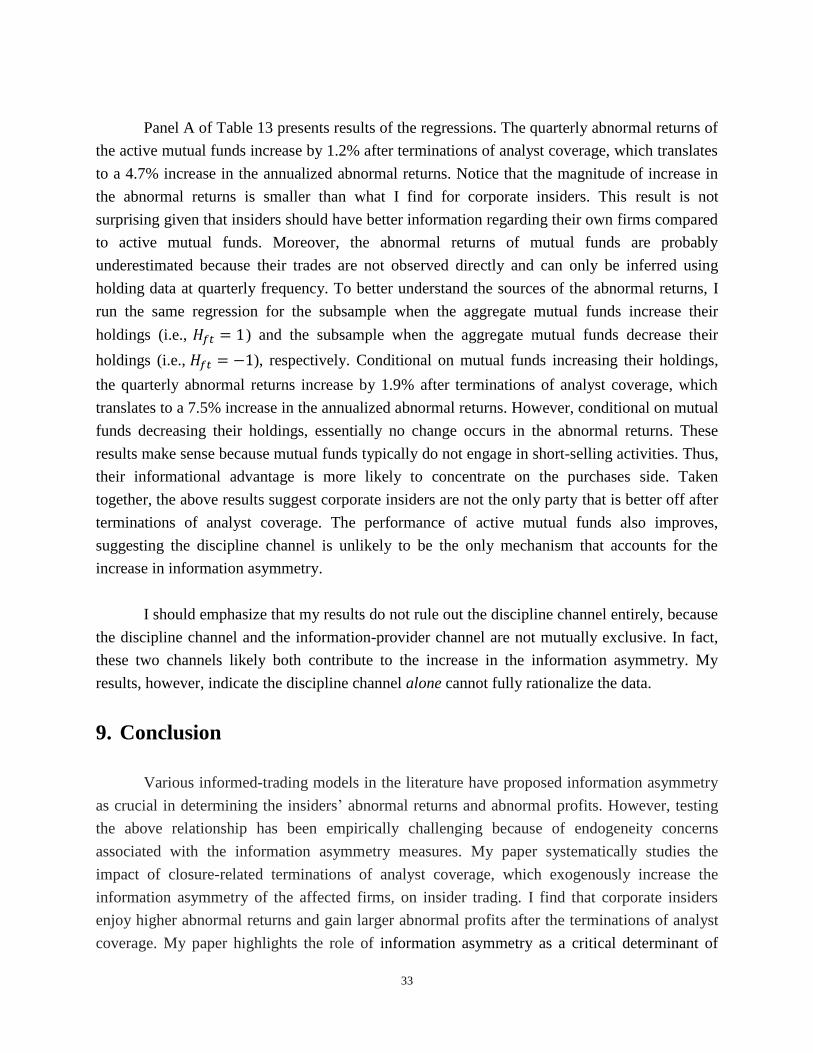
33
Panel A of Table 13 presents results of the regressions. The quarterly abnormal returns of
the active mutual funds increase by 1.2% after terminations of analyst coverage, which translates
to a 4.7% increase in the annualized abnormal returns. Notice that the magnitude of increase in
the abnormal returns is smaller than what I find for corporate insiders. This result is not
surprising given that insiders should have better information regarding their own firms compared
to active mutual funds. Moreover, the abnormal returns of mutual funds are probably
underestimated because their trades are not observed directly and can only be inferred using
holding data at quarterly frequency. To better understand the sources of the abnormal returns, I
run the same regression for the subsample when the aggregate mutual funds increase their
holdings (i.e., ) and the subsample when the aggregate mutual funds decrease their
holdings (i.e., ), respectively. Conditional on mutual funds increasing their holdings,
the quarterly abnormal returns increase by 1.9% after terminations of analyst coverage, which
translates to a 7.5% increase in the annualized abnormal returns. However, conditional on mutual
funds decreasing their holdings, essentially no change occurs in the abnormal returns. These
results make sense because mutual funds typically do not engage in short-selling activities. Thus,
their informational advantage is more likely to concentrate on the purchases side. Taken
together, the above results suggest corporate insiders are not the only party that is better off after
terminations of analyst coverage. The performance of active mutual funds also improves,
suggesting the discipline channel is unlikely to be the only mechanism that accounts for the
increase in information asymmetry.
I should emphasize that my results do not rule out the discipline channel entirely, because
the discipline channel and the information-provider channel are not mutually exclusive. In fact,
these two channels likely both contribute to the increase in the information asymmetry. My
results, however, indicate the discipline channel alone cannot fully rationalize the data.
9. Conclusion
Various informed-trading models in the literature have proposed information asymmetry
as crucial in determining the insiders’ abnormal returns and abnormal profits. However, testing
the above relationship has been empirically challenging because of endogeneity concerns
associated with the information asymmetry measures. My paper systematically studies the
impact of closure-related terminations of analyst coverage, which exogenously increase the
information asymmetry of the affected firms, on insider trading. I find that corporate insiders
enjoy higher abnormal returns and gain larger abnormal profits after the terminations of analyst
coverage. My paper highlights the role of information asymmetry as a critical determinant of

34
insiders’ abnormal profits, and indicates the descriptive validity of informed-trading models
applied to corporate insiders’ trades. It also calls for regulatory attention to corporate insiders’
transactions associated with high levels of information asymmetry.
References:
Aboody, David, and Baruch Lev, 2000, Information Asymmetry, R&D, and Insider Gains, Journal of Finance
55, 2747–2766.
Amihud, Yakov, 2002, Illiquidity and Stock Returns: Cross-section and Time-series Effects, Journal of
Financial Markets 5, 31–56.
Back K., 1992, Insider Trading in Continuous Time, Review of Financial Studies 5, 387–409.
Balakrishnan, Karthik, Mary Billings, Bryan Kelly, and Alexander Ljungqvist, 2012, Shaping Liquidity: On
the Causal Effects of Voluntary Disclosure, Journal of Finance, forthcoming.
Barber, B., R. Lehavy, M. McNichols, and B. Trueman, 2001, Can investors profit from the prophets?
Consensus analyst recommendations and stock returns, Journal of Finance 56, 531–563.
Bettis, Carr, Don Vickery, and Donn W. Vickery, 1997, Mimickers of corporate insiders who make large-
volume trades, Financial Analysts Journal 53, 57–66.
Bhattacharya, U., 2014. Insider trading controversies: a literature review. In: Lo, A., Merton, R. (Ed.), Annual
Reviews of Financial Economics, forthcoming.
Brochet, F. 2010, Information content of insider trades before and after the Sarbanes–Oxley Act. Accounting
Review 85 (2): 419–446.
Brown, Lawrence D., Andrew C. Call, Michael B. Clement, and Nathan Y. Sharp, 2014, Insider the “black box”
of sell-side financial analysts, working paper.
Bushee, B.J., 1998, The influence of institutional investors on myopic R&D investment behavior. Accounting Review, 305–333.
Carhart, Mark, 1997, On Persistence in Mutual Fund Performance, Journal of Finance 52, 57–82.
Chen, Tao, Jarrad Harford, and Chen Lin, 2013, Do Financial Analysts Play a Monitoring Role? Evidence
from Natural Experiments, Journal of Financial Economics, forthcoming.
Cohen, Lauren, Christopher Malloy, and Lukasz Pomorski, 2012, Decoding Inside Information, Journal of
Finance 67, 1009–1043.
Copeland, Thomas E, and Dan Galai, 1983, Information Effects on the Bid-Ask Spread, Journal of Finance 38,
1457.

35
Daniel, Kent, Mark Grinblatt, Sheridan Titman, and Russ Wermers, 1997, Measuring mutual fund
performance with characteristic-based benchmarks, Journal of Finance 52, 1035–1058.
Del Guercio, Diane, Elizabeth R. Odders-White, and Mark J. Ready, 2013. The Deterrence effect of SEC
enforcement intensity on illegal insider trading, working paper.
Derrien, François, and Ambrus Kecskes, 2013, The Real Effects of Financial Shocks : Evidence from
Exogenous Changes in Analyst Coverage, Journal of Finance, 68, 1407–1440.
Derrien, François, Ambrus Kecskes, and Sattar Mansi, 2012, Information Asymmetry, the Cost of Debt, and
Credit Events, working paper.
Dyck, Alexander, Adair Morse, and Luigi Zingales, 2010, Who Blows the Whistle on Corporate Fraud?,
Journal of Finance 65, 2213–2253.
Fama, Eugene F, and Kenneth R French, 1992, The Cross-Section of Expected Stock Returns, Journal of
Finance 47, 427–465.
Fong, Kingsley Y. L., Harrison G. Hong, Marcin T. Kacperczyk, and Jeffrey D. Kubik, 2011, Do Security
Analysts Discipline Credit Rating Agencies?, working paper.
Gleason, Cristi A., and Charles M.C. Lee, 2003, Analyst forecast revisions and market price discovery,
Accounting Review 78, 193–225.
Grossman, Sanford, and Joseph Stiglitz, 1980, On the Impossibility of Informationally Efficient Markets, . Ed.
Sanford J Grossman American Economic Review 70, 393–408.
Hong, H, and M Kacperczyk, 2010, Competition and Bias, The Quarterly Journal of Economics 125, 1683–
1725.
Huddart, Steven J., and Bin Ke, 2007, Information Asymmetry and Cross-sectional Variation in Insider
Trading, Contemporary Accounting Research 24, 195–232.
Irani, Rustom M., and David Oesch, 2013, Monitoring and Corporate Disclosure: Evidence from a Natural
Experiment, Journal of Financial Economics, 109, 398–418.
Jegadeesh, Narasimhan, Joonghyuk Kim, Susan Krische, and Charles Lee, 2004, Analyzing the analysts:
When do recommendations add value? Journal of Finance 59, 1083–1124.
Jeng, Leslie A, Andrew Metrick, and Richard Zeckhauser, 2003, Estimating the Returns to Insider Trading: A
Performance-evaluation Perspective, The Review of Economics and Statistics 85, 453–471.
Johnson, L. Travis, and Eric C. So, 2014, A Simple Multimarket Measure of Information Asymmetry, working
paper.

36
Karamanou, Irene, Grace Pownall, Rachna Prakash, 2013, Asymmetric information consolidation and price
discovery: inferring bad news from insider sales, working paper.
Ke, Bin, Steven Huddart, and Kathy Petroni, 2003, What Insiders Know about Future Earnings and How They
Use It: Evidence from Insider Trades, Journal of Accounting and Economics 35, 315–346.
Kelly, B., and a. Ljungqvist, 2012, Testing Asymmetric-Information Asset Pricing Models, Review of
Financial Studies 25, 1366–1413.
Kyle, Albert S, 1985, Continuous Auctions and Insider Trading, Econometrica 53, 1315–1335.
Lakonishok, Josef, and Inmoo Lee, 2001, Are Insider Trades Informative?, Review of Financial Studies 14,
79–111.
Leland, Hayne, 1992, Insider trading: Should it be prohibited? Journal of Political Economy 100, 859–887.
Pastor, Lubos, and Robert F Stambaugh, 2003, Liquidity risk and expected stock returns, Journal of Political
Economy 111, 642–685.
Piotroski, Joseph D, and Darren T Roulstone, 2005, Do insider trades reflect both contrarian beliefs and
superior knowledge about future cash flow realizations?, Journal of Accounting and Economics 39, 55–81.
Rozeff, Michael S, and Mir A Zaman, 1998, Overreaction and Insider Trading: Evidence from Growth and
Value Portfolios, Journal of Finance 53, 701–716.
Seyhun, H. Nejat, 1986, Insiders’ Profits, Costs of Trading, and Market Efficiency, Journal of Financial
Economics 16, 189–212.
Spiegel, Matthew, and Avanidhar Subrahmanyam, 1992, Informed Speculation and Hedging in a
Noncompetitive Securities Market, Review of Financial Studies 5, 307–329.
Wermers, Russ, 2004, Is money really ‘smart’? New evidence on the relation between mutual fund flows,
manager behavior, and performance persistence, working paper.
Womack, Kent L., 1996, Do brokerage analysts’ recommendations have investment value? Journal of Finance
51, 137–168.
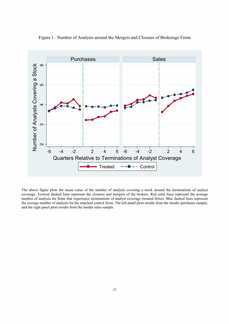
37
Figure 1. Number of Analysts around the Mergers and Closures of Brokerage Firms
The above figure plots the mean value of the number of analysts covering a stock around the terminations of analyst coverage. Vertical dashed lines represent the closures and mergers of the brokers. Red solid lines represent the average number of analysts for firms that experience terminations of analyst coverage (treated firms). Blue dashed lines represent the average number of analysts for the matched control firms. The left panel plots results from the insider purchases sample, and the right panel plots results from the insider sales sample.
23
45
6
-6 -4 -2 2 4 6 -6 -4 -2 2 4 6
Purchases Sales
Treated Control
Number of Analysts Covering a Stock
Quarters Relative to Terminations of Analyst Coverage
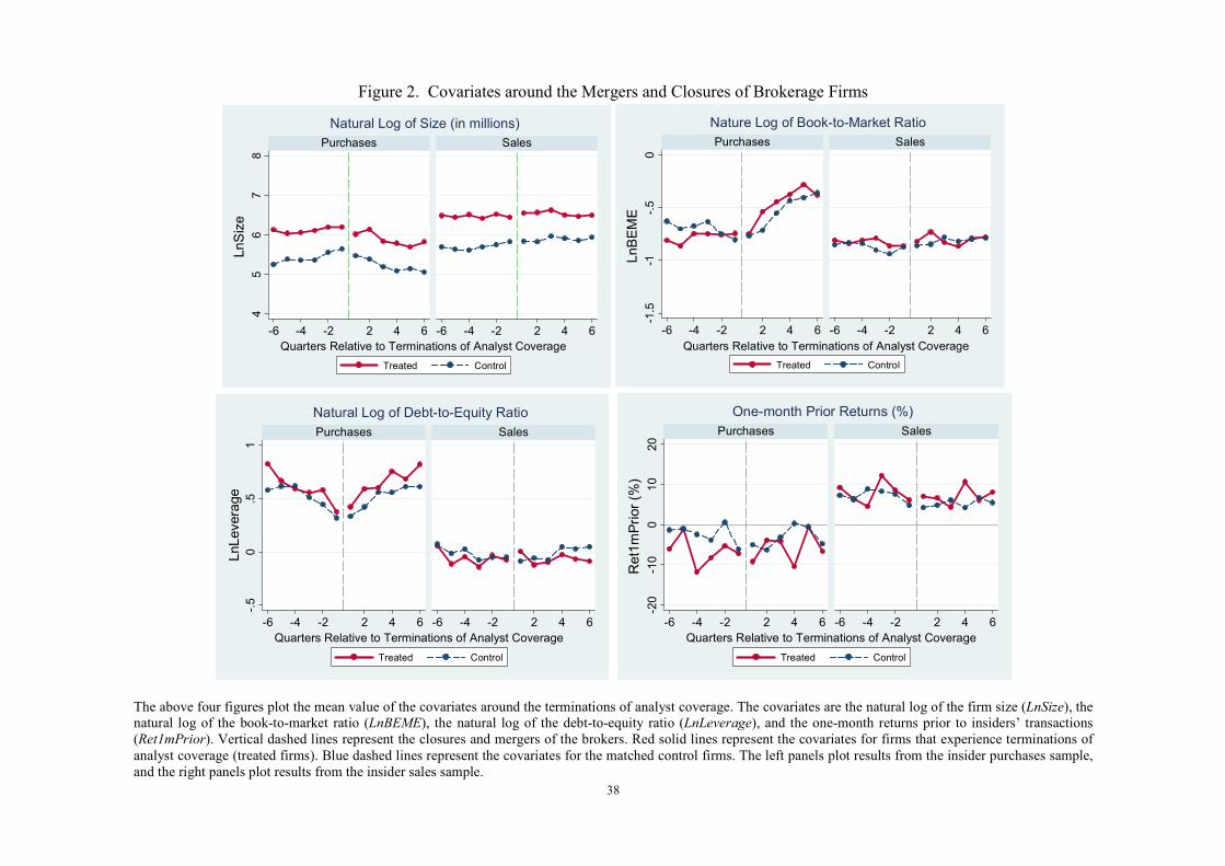
38
Figure 2. Covariates around the Mergers and Closures of Brokerage Firms
The above four figures plot the mean value of the covariates around the terminations of analyst coverage. The covariates are the natural log of the firm size (LnSize), the natural log of the book-to-market ratio (LnBEME), the natural log of the debt-to-equity ratio (LnLeverage), and the one-month returns prior to insiders’ transactions (Ret1mPrior). Vertical dashed lines represent the closures and mergers of the brokers. Red solid lines represent the covariates for firms that experience terminations of analyst coverage (treated firms). Blue dashed lines represent the covariates for the matched control firms. The left panels plot results from the insider purchases sample, and the right panels plot results from the insider sales sample.
45
67
8
-6 -4 -2 2 4 6 -6 -4 -2 2 4 6
Purchases Sales
Treated Control
LnSize
Quarters Relative to Terminations of Analyst Coverage
Natural Log of Size (in millions)
-1.5
-1-.5
0
-6 -4 -2 2 4 6 -6 -4 -2 2 4 6
Purchases Sales
Treated Control
LnBEME
Quarters Relative to Terminations of Analyst Coverage
Nature Log of Book-to-Market Ratio
-.5
0.5
1
-6 -4 -2 2 4 6 -6 -4 -2 2 4 6
Purchases Sales
Treated Control
LnLeverage
Quarters Relative to Terminations of Analyst Coverage
Natural Log of Debt-to-Equity Ratio
-20
-10
010
20
-6 -4 -2 2 4 6 -6 -4 -2 2 4 6
Purchases Sales
Treated Control
Ret1mPrior (%
)Quarters Relative to Terminations of Analyst Coverage
One-month Prior Returns (%)
39
Figure 3. Insiders’ Abnormal Returns around the Mergers and Closures of Brokerage Firms
The above two figures plot the average three-month (upper panel) and six-month (lower panel) cumulative abnormal returns for insider transactions that take place in different quarters relative to the terminations of analyst coverage. For example, the first red dot (from left) in the left upper panel represents the mean value of the three-month cumulative abnormal returns for all insider purchases that take place six quarters prior to the closures and mergers of the brokers, and come from firms experiencing terminations of analyst coverage. The cumulative abnormal returns are estimated by Carhart’s four-factor model. Vertical dashed lines represent the closures and mergers of the brokers. Red solid lines represent the cumulative abnormal returns for firms that experience terminations of analyst coverage (treated firms). Blue dashed lines represent the cumulative abnormal returns for the matched control firms. The left panels plot results from the insider purchases sample, and the right panels plot results from the insider sales sample. Notice that negative abnormal returns for insider sales represent losses the insiders avoid.
-10
010
20
-6 -4 -2 2 4 6 -6 -4 -2 2 4 6
Purchases Sales
Three-month CAR (%)
Treated Control
CAR_3m (%)
Quarters Relative to Terminations of Analyst Coverage
-20
020
40
-6 -4 -2 2 4 6 -6 -4 -2 2 4 6
Purchases Sales
Six-month CAR (%)
Treated Control
CAR_6m (%)
Quarters Relative to Terminations of Analyst Coverage
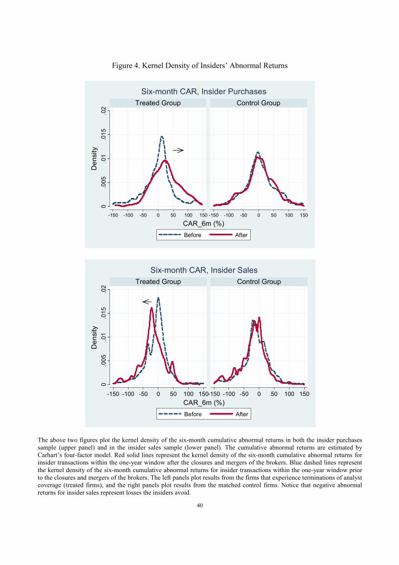
40
Figure 4. Kernel Density of Insiders’ Abnormal Returns
The above two figures plot the kernel density of the six-month cumulative abnormal returns in both the insider purchases sample (upper panel) and in the insider sales sample (lower panel). The cumulative abnormal returns are estimated by Carhart’s four-factor model. Red solid lines represent the kernel density of the six-month cumulative abnormal returns for insider transactions within the one-year window after the closures and mergers of the brokers. Blue dashed lines represent the kernel density of the six-month cumulative abnormal returns for insider transactions within the one-year window prior to the closures and mergers of the brokers. The left panels plot results from the firms that experience terminations of analyst coverage (treated firms), and the right panels plot results from the matched control firms. Notice that negative abnormal returns for insider sales represent losses the insiders avoid.
0.005
.01
.015
.02
-150 -100 -50 0 50 100 150 -150 -100 -50 0 50 100 150
Treated Group Control Group
Before After
Density
CAR_6m (%)
Six-month CAR, Insider Purchases
0.005
.01
.015
.02
-150 -100 -50 0 50 100 150-150 -100 -50 0 50 100 150
Treated Group Control Group
Before After
Density
CAR_6m (%)
Six-month CAR, Insider Sales

41
Table 1. Ex-ante Summary Statistics
This table presents ex-ante summary statistics for both the treated group and the matched control group. The treated firms
are firms that experience closure-related terminations of analyst coverage. Each treated firm is matched with up to five
control firms in the same Fama-French size and book-to-market quintile. If more than five candidate firms exist, those with
the closest bid-ask spreads prior to the terminations of analyst coverage are chosen. Summary statistics are calculated at the
firm level using observations in the one-year period prior to the terminations of analyst coverage. LnSize is the natural log
of market cap (in millions) in year t-1; LnBEME is the natural log of book-to-market ratio in year t-1; LnLev is the natural
log of debt-to-equity ratio in year t-1; Spreads is the one-month (day -21 to day -1) average percentage bid-ask spreads
prior to the insider transactions, where the percentage bid-ask spreads are calculated by
; Ret1mPrior is the
one-month (day -21 to day -1) cumulative raw returns prior to insider transactions; CAR1m, CAR3m, and CAR6m are the
cumulative abnormal returns adjusted by the Carhart four-factor model over one month, three months, and six months,
respectively, after the insider transactions; LnShares is the natural log of the transaction shares, and LnValue is the natural
log of the transaction value. The treated firms are limited to firms that have five or fewer analysts covering the firm prior to
coverage reductions. Negative abnormal returns for insider sales represent losses that the insiders avoid. The data span
1999-2008.
Panel A. Insider purchases.
Treated Group
Control Group
(# of firms = 129)
(# of firms = 529)
(# of trades = 2599)
(# of trades = 9422)
mean std. dev.
mean std. dev. p-value
# of Coverage 4.03 2.07
3.78 2.95 0.36
Spreads (%) 1.81 1.92
1.81 1.83 0.94
LnSize 6.17 1.48
5.47 1.30 0.00***
LnBEME -0.85 1.00
-0.85 0.95 0.95
LnLev 0.51 1.45
0.47 1.55 0.79
Ret1mPrior (%) -7.44 19.56
-4.89 18.14 0.16
CAR1m (%) 2.10 13.39
2.42 15.63 0.83
CAR3m (%) 4.01 29.20
4.46 27.86 0.71
CAR6m (%) 2.45 48.82
5.31 47.96 0.64
LnShares 7.42 1.98
7.40 2.02 0.92
LnValue 9.94 1.86 9.89 1.78 0.80
Panel B. Insider sales.
Treated Group
Control Group
(# of firms = 231)
(# of firms = 758)
(# of trades = 11809)
(# of trades = 42173)
mean std. dev.
mean std. dev. p-value
# of Coverage 4.34 2.36
4.21 2.09 0.42
Spreads (%) 0.51 0.59
0.56 0.73 0.34
LnSize 6.56 1.31
5.88 1.11 0.00***
LnBEME -0.99 0.79
-0.93 0.81 0.32
LnLev -0.08 1.45
-0.04 1.47 0.72
Ret1mPrior (%) 5.79 12.72
6.60 15.85 0.48
CAR1m (%) -1.26 9.23
-2.19 12.53 0.30
CAR3m (%) -4.17 22.13
-6.21 24.66 0.26
CAR6m (%) -6.25 35.77
-10.53 43.28 0.17
LnShares 7.53 1.84
7.44 1.73 0.50
LnValue 10.72 2.09 10.55 1.91 0.20
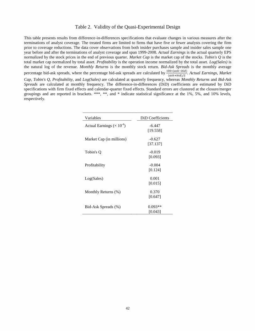
42
Table 2. Validity of the Quasi-Experimental Design
This table presents results from difference-in-differences specifications that evaluate changes in various measures after the
terminations of analyst coverage. The treated firms are limited to firms that have five or fewer analysts covering the firm
prior to coverage reductions. The data cover observations from both insider purchases sample and insider sales sample one
year before and after the terminations of analyst coverage and span 1999-2008. Actual Earnings is the actual quarterly EPS
normalized by the stock prices in the end of previous quarter. Market Cap is the market cap of the stocks. Tobin's Q is the
total market cap normalized by total asset. Profitability is the operation income normalized by the total asset. Log(Sales) is
the natural log of the revenue. Monthly Returns is the monthly stock return. Bid-Ask Spreads is the monthly average
percentage bid-ask spreads, where the percentage bid-ask spreads are calculated by
. Actual Earnings, Market
Cap, Tobin's Q, Profitability, and Log(Sales) are calculated at quarterly frequency, whereas Monthly Returns and Bid-Ask
Spreads are calculated at monthly frequency. The difference-in-differences (DiD) coefficients are estimated by DiD
specifications with firm fixed effects and calendar-quarter fixed effects. Standard errors are clustered at the closure/merger
groupings and are reported in brackets. ***, **, and * indicate statistical significance at the 1%, 5%, and 10% levels,
respectively.
Variables
DiD Coefficients
Actual Earnings (× 10-4
) -6.447
[19.558]
Market Cap (in millions)
-0.627
[37.137]
Tobin's Q
-0.019
[0.093]
Profitability
-0.004
[0.124]
Log(Sales)
0.001
[0.015]
Monthly Returns (%)
0.370
[0.647]
Bid-Ask Spreads (%)
0.093**
[0.043]

43
Table 3. Insiders’ Abnormal Returns
This table presents results from difference-in-differences specifications that evaluate changes in insiders’ abnormal returns
after the terminations of analyst coverage. The dependent variables are insiders’ cumulative abnormal returns adjusted by
the Carhart four-factor model over one month (CAR1m), three months (CAR3m), and six months (CAR6m) after the insider
transactions. Treat is a dummy variable that equals 1 if the transaction comes from treated firms. Post is a dummy variable
that equals 1 if the transaction happens after terminations of analyst coverage. Control variables include LnSize, LnBEME,
LnLev, and Ret1mPrior, which are defined in Table 1. Standard errors are clustered at the closure/merger groupings and are
reported in brackets. ***, **, and * indicate statistical significance at the 1%, 5%, and 10% levels, respectively. The treated
firms are limited to firms that have five or fewer analysts covering the firm prior to coverage reductions. Negative abnormal
returns for insider sales represent losses that the insiders avoid. The data cover insider transactions one year before and after
the terminations of analyst coverage and span 1999-2008.
Panel A. Insider purchases.
(1) (2) (3) (4) (5) (6)
CAR1m (%) CAR1m (%) CAR3m (%) CAR3m (%) CAR6m (%) CAR6m (%)
Treat × Post 6.92*** 7.97** 10.47*** 9.86*** 15.96*** 18.35***
[2.02] [3.68] [3.32] [2.75] [4.72] [6.21]
LnSize 3.86 8.45* 3.42 10.55 -0.10 21.02*
[3.88] [4.87] [4.58] [7.16] [9.57] [10.83]
LnBEME 7.91** 10.46** 20.89*** 21.02*** 38.23*** 45.65***
[3.80] [4.68] [5.73] [7.81] [10.39] [12.44]
LnLev 2.80 4.20 1.38 7.34 -3.32 5.05
[2.09] [2.90] [5.72] [7.10] [8.59] [9.81]
Ret1mPrior -0.12*** -0.14*** -0.14*** -0.15*** -0.17*** -0.25***
[0.02] [0.03] [0.04] [0.05] [0.05] [0.06]
Fixed effect 1 calendar dates calendar dates calendar dates calendar dates calendar dates calendar dates
Fixed effect 2 firm firm × insider firm firm × insider firm firm × insider
# of transactions 24078 24078 24008 24008 23726 23726
R-squared 0.47 0.65 0.57 0.74 0.67 0.82
Panel B. Insider sales.
(1) (2) (3) (4) (5) (6)
CAR1m (%) CAR1m (%) CAR3m (%) CAR3m (%) CAR6m (%) CAR6m (%)
Treat × Post -2.49* -2.89** -6.11** -6.05** -10.73*** -10.17**
[1.42] [1.33] [2.58] [2.66] [3.74] [4.46]
LnSize -5.79*** -5.01** -7.25* -6.45 -7.78 -9.39
[2.01] [1.96] [4.02] [4.76] [6.30] [6.94]
LnBEME 2.24 2.50 5.67* 4.09 12.62** 8.63
[1.71] [1.58] [3.44] [3.78] [5.06] [5.91]
LnLev 0.38 0.75 0.18 1.43 2.37 1.86
[1.33] [1.42] [3.26] [3.62] [5.20] [5.49]
Ret1mPrior -0.08*** -0.10*** -0.09** -0.09 -0.11* -0.14**
[0.03] [0.03] [0.04] [0.06] [0.06] [0.07]
Fixed effect 1 calendar dates calendar dates calendar dates calendar dates calendar dates calendar dates
Fixed effect 2 firm firm × insider firm firm × insider firm firm × insider
# of transactions 103330 103330 102838 102838 101908 101908
R-squared 0.48 0.63 0.59 0.74 0.64 0.77
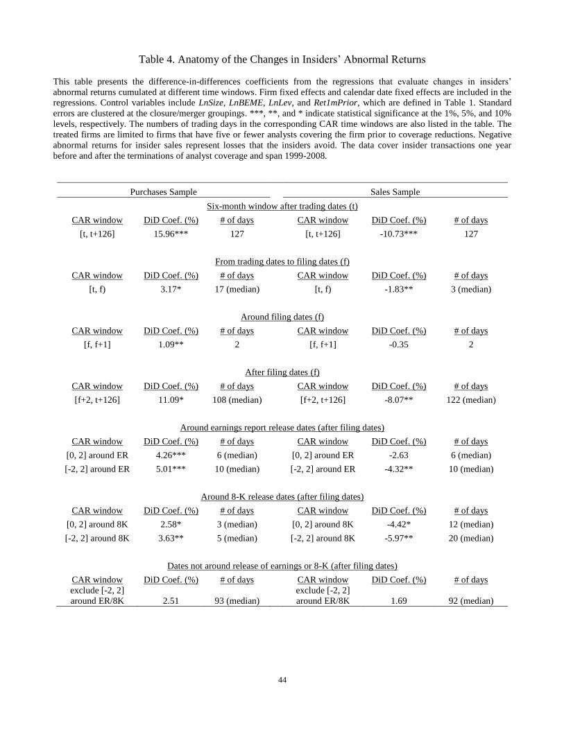
44
Table 4. Anatomy of the Changes in Insiders’ Abnormal Returns
This table presents the difference-in-differences coefficients from the regressions that evaluate changes in insiders’
abnormal returns cumulated at different time windows. Firm fixed effects and calendar date fixed effects are included in the
regressions. Control variables include LnSize, LnBEME, LnLev, and Ret1mPrior, which are defined in Table 1. Standard
errors are clustered at the closure/merger groupings. ***, **, and * indicate statistical significance at the 1%, 5%, and 10%
levels, respectively. The numbers of trading days in the corresponding CAR time windows are also listed in the table. The
treated firms are limited to firms that have five or fewer analysts covering the firm prior to coverage reductions. Negative
abnormal returns for insider sales represent losses that the insiders avoid. The data cover insider transactions one year
before and after the terminations of analyst coverage and span 1999-2008.
Purchases Sample Sales Sample
Six-month window after trading dates (t)
CAR window DiD Coef. (%) # of days
CAR window DiD Coef. (%) # of days
[t, t+126] 15.96*** 127
[t, t+126] -10.73*** 127
From trading dates to filing dates (f)
CAR window DiD Coef. (%) # of days
CAR window DiD Coef. (%) # of days
[t, f) 3.17* 17 (median)
[t, f) -1.83** 3 (median)
Around filing dates (f)
CAR window DiD Coef. (%) # of days
CAR window DiD Coef. (%) # of days
[f, f+1] 1.09** 2
[f, f+1] -0.35 2
After filing dates (f)
CAR window DiD Coef. (%) # of days
CAR window DiD Coef. (%) # of days
[f+2, t+126] 11.09* 108 (median)
[f+2, t+126] -8.07** 122 (median)
Around earnings report release dates (after filing dates)
CAR window DiD Coef. (%) # of days
CAR window DiD Coef. (%) # of days
[0, 2] around ER 4.26*** 6 (median)
[0, 2] around ER -2.63 6 (median)
[-2, 2] around ER 5.01*** 10 (median)
[-2, 2] around ER -4.32** 10 (median)
Around 8-K release dates (after filing dates)
CAR window DiD Coef. (%) # of days
CAR window DiD Coef. (%) # of days
[0, 2] around 8K 2.58* 3 (median)
[0, 2] around 8K -4.42* 12 (median)
[-2, 2] around 8K 3.63** 5 (median)
[-2, 2] around 8K -5.97** 20 (median)
Dates not around release of earnings or 8-K (after filing dates)
CAR window DiD Coef. (%) # of days
CAR window DiD Coef. (%) # of days
exclude [-2, 2]
around ER/8K 2.51 93 (median)
exclude [-2, 2]
around ER/8K 1.69 92 (median)
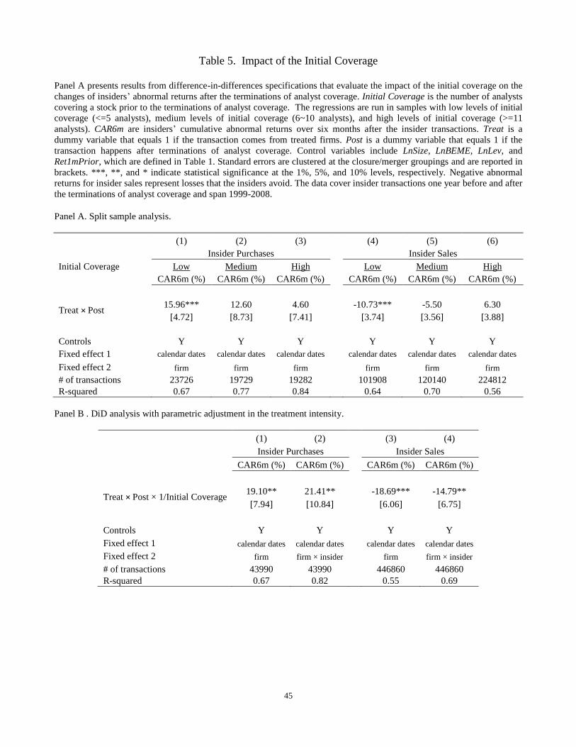
45
Table 5. Impact of the Initial Coverage
Panel A presents results from difference-in-differences specifications that evaluate the impact of the initial coverage on the
changes of insiders’ abnormal returns after the terminations of analyst coverage. Initial Coverage is the number of analysts
covering a stock prior to the terminations of analyst coverage. The regressions are run in samples with low levels of initial
coverage (<=5 analysts), medium levels of initial coverage (6~10 analysts), and high levels of initial coverage (>=11
analysts). CAR6m are insiders’ cumulative abnormal returns over six months after the insider transactions. Treat is a
dummy variable that equals 1 if the transaction comes from treated firms. Post is a dummy variable that equals 1 if the
transaction happens after terminations of analyst coverage. Control variables include LnSize, LnBEME, LnLev, and
Ret1mPrior, which are defined in Table 1. Standard errors are clustered at the closure/merger groupings and are reported in
brackets. ***, **, and * indicate statistical significance at the 1%, 5%, and 10% levels, respectively. Negative abnormal
returns for insider sales represent losses that the insiders avoid. The data cover insider transactions one year before and after
the terminations of analyst coverage and span 1999-2008.
Panel A. Split sample analysis.
(1) (2) (3) (4) (5) (6)
Insider Purchases
Insider Sales
Initial Coverage Low Medium High
Low Medium High
CAR6m (%) CAR6m (%) CAR6m (%)
CAR6m (%) CAR6m (%) CAR6m (%)
Treat × Post 15.96*** 12.60 4.60
-10.73*** -5.50 6.30
[4.72] [8.73] [7.41]
[3.74] [3.56] [3.88]
Controls Y Y Y
Y Y Y
Fixed effect 1 calendar dates calendar dates calendar dates
calendar dates calendar dates calendar dates
Fixed effect 2 firm firm firm
firm firm firm
# of transactions 23726 19729 19282
101908 120140 224812
R-squared 0.67 0.77 0.84 0.64 0.70 0.56
Panel B . DiD analysis with parametric adjustment in the treatment intensity.
(1) (2) (3) (4)
Insider Purchases
Insider Sales
CAR6m (%) CAR6m (%)
CAR6m (%) CAR6m (%)
Treat × Post × 1/Initial Coverage 19.10** 21.41**
-18.69*** -14.79**
[7.94] [10.84]
[6.06] [6.75]
Controls Y Y
Y Y
Fixed effect 1 calendar dates calendar dates
calendar dates calendar dates
Fixed effect 2 firm firm × insider
firm firm × insider
# of transactions 43990 43990
446860 446860
R-squared 0.67 0.82 0.55 0.69
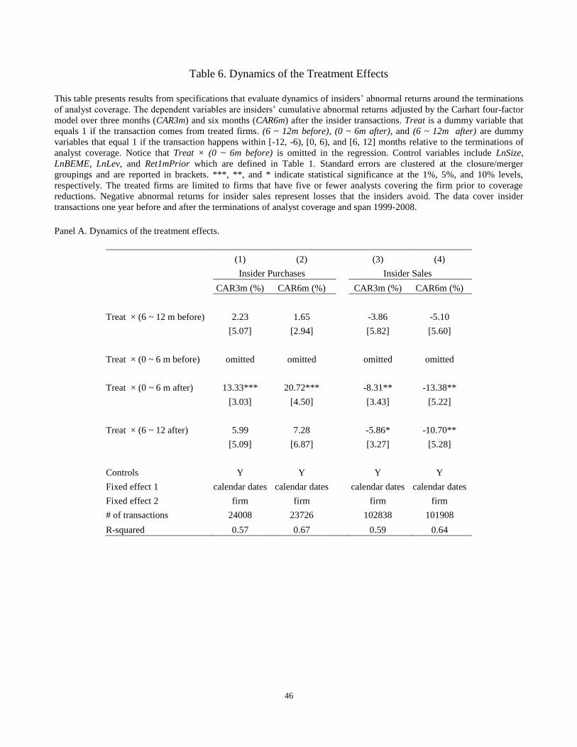
46
Table 6. Dynamics of the Treatment Effects
This table presents results from specifications that evaluate dynamics of insiders’ abnormal returns around the terminations
of analyst coverage. The dependent variables are insiders’ cumulative abnormal returns adjusted by the Carhart four-factor
model over three months (CAR3m) and six months (CAR6m) after the insider transactions. Treat is a dummy variable that
equals 1 if the transaction comes from treated firms. (6 ~ 12m before), (0 ~ 6m after), and (6 ~ 12m after) are dummy
variables that equal 1 if the transaction happens within [-12, -6), [0, 6), and [6, 12] months relative to the terminations of
analyst coverage. Notice that Treat × (0 ~ 6m before) is omitted in the regression. Control variables include LnSize,
LnBEME, LnLev, and Ret1mPrior which are defined in Table 1. Standard errors are clustered at the closure/merger
groupings and are reported in brackets. ***, **, and * indicate statistical significance at the 1%, 5%, and 10% levels,
respectively. The treated firms are limited to firms that have five or fewer analysts covering the firm prior to coverage
reductions. Negative abnormal returns for insider sales represent losses that the insiders avoid. The data cover insider
transactions one year before and after the terminations of analyst coverage and span 1999-2008.
Panel A. Dynamics of the treatment effects.
(1) (2) (3) (4)
Insider Purchases
Insider Sales
CAR3m (%) CAR6m (%)
CAR3m (%) CAR6m (%)
Treat × (6 ~ 12 m before) 2.23 1.65
-3.86 -5.10
[5.07] [2.94]
[5.82] [5.60]
Treat × (0 ~ 6 m before) omitted omitted
omitted omitted
Treat × (0 ~ 6 m after) 13.33*** 20.72***
-8.31** -13.38**
[3.03] [4.50]
[3.43] [5.22]
Treat × (6 ~ 12 after) 5.99 7.28
-5.86* -10.70**
[5.09] [6.87]
[3.27] [5.28]
Controls Y Y
Y Y
Fixed effect 1 calendar dates calendar dates
calendar dates calendar dates
Fixed effect 2 firm firm
firm firm
# of transactions 24008 23726
102838 101908
R-squared 0.57 0.67 0.59 0.64

47
Table 6. Dynamics of the Treatment Effects (continued)
Panel B. Impact of the recovery of the number of analysts on the dynamics of the treatment effects.
I calculate the recovery in the number of analysts by subtracting the number of analysts right after the terminations from the
number of analysts six months after the terminations. Treated firms are sorted into two groups based on this measure. I
perform the sorting annually and independently of the number of analysts prior to the terminations to ensure the two groups
of firms have the same treatment intensity. Strong_Analyst_Recovery is a dummy variable that equals 1 if a firm’s recovery
in the number of analysts is larger than the median values.
(1) (2) (3) (4) (5) (6)
Insider Purchases
Insider Sales
CAR6m (%) CAR6m (%) CAR6m (%)
CAR6m (%) CAR6m (%) CAR6m (%)
Treat × (0 ~ 6 m after) 21.49** 19.23*** 24.55**
-15.52** -13.39** -18.31*
[9.37] [4.39] [10.12]
[7.54] [6.65] [10.41]
Treat × (0 ~ 6 m after) × -6.11
-16.17
6.26
13.68
Strong_Analyst_Recovery [17.25]
[18.82]
[13.17]
[12.94]
Treat × (6 ~ 12 m after) 6.26 16.68* 18.92*
-12.09** -18.44*** -20.61***
[6.87] [9.95] [10.93]
[6.02] [4.52] [5.65]
Treat × (6 ~ 12 m after) ×
-25.48* -27.42**
17.86* 23.82***
Strong_Analyst_Recovery
[13.43] [13.52]
[9.26] [8.56]
Controls Y Y Y
Y Y Y
Fixed effect 1 calendar dates calendar dates calendar dates
calendar dates calendar dates calendar dates
Fixed effect 2 firm firm firm
firm firm firm
# of observations 23726 23726 23726
101908 101908 101908
R-squared 0.67 0.67 0.67 0.64 0.64 0.64

48
Table 7. Portfolio Return Analysis
This table presents the performance-evaluation results for insider portfolios before and after the terminations of analyst
coverage. Insider transactions from firms that have five or fewer analysts prior to coverage reductions are included in the
portfolios. The holding periods of the insider transactions are one month, three months, and six months. Insider transactions
are weighted either equally or by treatment intensity (1/ the number of the initial coverage). The dependent variables are
excess portfolio returns. The independent variables include RMRF, SMB, HML, and MOM, which are daily factors
downloaded from Kenneth French’s website. α is the regression intercept. Annualized α = 252*α and Sharpe ratio
=
. Standard errors are robust to heteroskedasticity. ***, **, and * indicate statistical significance
at 1%, 5%, and 10% levels, respectively. The negative alpha and Sharpe ratio for insider sales represent losses that the
insiders avoid. The sample is from 2000/5/1 to 2007/12/3 (a common period shared by all subsamples).
Panel A. Portfolios constructed based on insider purchases one year before coverage reductions.
(1) (2) (3) (4) (5) (6)
Excess Portfolio Returns of Insider Purchases (%)
Holding Period 1 month 1 month 3 months 3 months 6 months 6 months
Weighting Method Equal 1/Coverage Equal 1/Coverage Equal 1/Coverage
α 0.03 0.03 0.03 0.06 0.02 0.02
[0.04] [0.05] [0.04] [0.05] [0.04] [0.04]
Sharpe ratio 0.37 0.34 0.42 0.55 0.34 0.32
Annualized α (%) 7.15 7.16 7.53 13.78 4.43 4.54
# of trading days 1909 1909 1909 1909 1909 1909
R-squared 0.23 0.16 0.29 0.20 0.36 0.28
Panel B. Portfolios constructed based on insider purchases one year after coverage reductions.
(1) (2) (3) (4) (5) (6)
Excess Portfolio Returns of Insider Purchase (%)
Holding Period 1 month 1 month 3 months 3 months 6 months 6 months
Weighting Method Equal 1/Coverage Equal 1/Coverage Equal 1/Coverage
α 0.12*** 0.11** 0.08*** 0.06* 0.08*** 0.07**
[0.04] [0.05] [0.03] [0.04] [0.03] [0.03]
Sharpe ratio 1.13 0.92 0.94 0.74 1.04 0.83
Annualized α (%) 30.43 28.00 19.49 15.62 20.19 16.57
# of trading days 1909 1909 1909 1909 1909 1909
R-squared 0.30 0.25 0.40 0.35 0.44 0.41

49
Table 7. Portfolio Return Analysis (continued)
Panel C. Portfolios constructed based on insider sales one year before coverage reductions.
(1) (2) (3) (4) (5) (6)
Excess Portfolio Returns of Insider Sales (%)
Holding Period 1 month 1 month 3 months 3 months 6 months 6 months
Weighting Method Equal 1/Coverage Equal 1/Coverage Equal 1/Coverage
α -0.01 0.02 0.03 0.05 0.02 0.03
[0.04] [0.04] [0.03] [0.04] [0.02] [0.03]
Sharpe ratio 0.07 0.17 0.40 0.40 0.34 0.24
Annualized α (%) -1.38 4.38 8.53 13.00 6.06 6.39
# of trading days 1909 1909 1909 1909 1909 1909
R-squared 0.42 0.39 0.56 0.49 0.65 0.58
Panel D. Portfolios constructed based on insider sales one year after coverage reductions.
(1) (2) (3) (4) (5) (6)
Excess Portfolio Returns of Insider Sales (%)
Holding Period 1 month 1 month 3 months 3 months 6 months 6 months
Weighting Method Equal 1/Coverage Equal 1/Coverage Equal 1/Coverage
α -0.09** -0.11*** -0.04 -0.06* -0.03 -0.05
[0.04] [0.04] [0.03] [0.03] [0.03] [0.03]
Sharpe ratio -0.56 -0.71 -0.19 -0.36 -0.14 -0.30
Annualized α (%) -22.85 -28.03 -9.58 -14.15 -7.09 -11.23
# of trading days 1909 1909 1909 1909 1909 1909
R-squared 0.46 0.45 0.58 0.56 0.66 0.63

50
Table 8. Insiders’ Trading Volume and Transaction Value
This table presents results from difference-in-differences specifications that evaluate changes in insiders’ trading volume
and transaction value after the terminations of analyst coverage. The dependent variables are the natural log of the
transaction shares (LnShares) and the natural log of insider transaction value (LnValue). Treat is a dummy variable that
equals 1 if the transaction comes from treated firms. Post is a dummy variable that equals 1 if the transaction happens after
the terminations of analyst coverage. Treated firms are sorted into two groups based on the bid-ask spreads prior to the
coverage reductions. I perform the sorting annually and independently of the number of analysts to ensure the two groups
of firms have the same treatment intensity. Liquid (LIlliquid) is a dummy variable that equals 1 if a firm’s average bid-ask
spreads are smaller (larger) than the median values. Control variables include LnSize, LnBEME, LnLev, and Ret1mPrior,
which are defined in Table 1. Standard errors are clustered at the closure/merger groupings and are reported in brackets.
***, **, and * indicate statistical significance at the 1%, 5%, and 10% levels, respectively. The treated firms are limited to
firms that have five or fewer analysts covering the firm prior to coverage reductions. The data cover insider transactions
one year before and after the terminations of analyst coverage and span 1999-2008.
Panel A. Insider purchases
(1) (2) (3) (4)
LnShares LnShares
LnValue LnValue
Treat × Post 0.19
0.16
[0.14]
[0.14]
Treat × Post × Liquid
0.49***
0.34***
[0.12]
[0.12]
Treat × Post × Illiquid
-0.06
0.01
[0.21]
[0.24]
Controls Y Y
Y Y
Fixed effect 1 calendar dates calendar dates
calendar dates calendar dates
Fixed effect 2 firm × insider firm × insider
firm × insider firm × insider
# of transactions 24857 24857
24857 24857
R-squared 0.77 0.77 0.74 0.74
Panel B. Insider sales
(1) (2) (3) (4)
LnShares LnShares
LnValue LnValue
Treat × Post 0.07
0.11
[0.07]
[0.11]
Treat × Post × Liquid
0.16***
0.17
[0.05]
[0.10]
Treat × Post × Illiquid
-0.03
0.03
[0.14]
[0.19]
Controls Y Y
Y Y
Fixed effect 1 calendar dates calendar dates
calendar dates calendar dates
Fixed effect 2 firm × insider firm × insider
firm × insider firm × insider
# of transactions 109183 109183
109183 109183
R-squared 0.62 0.62 0. 65 0.65
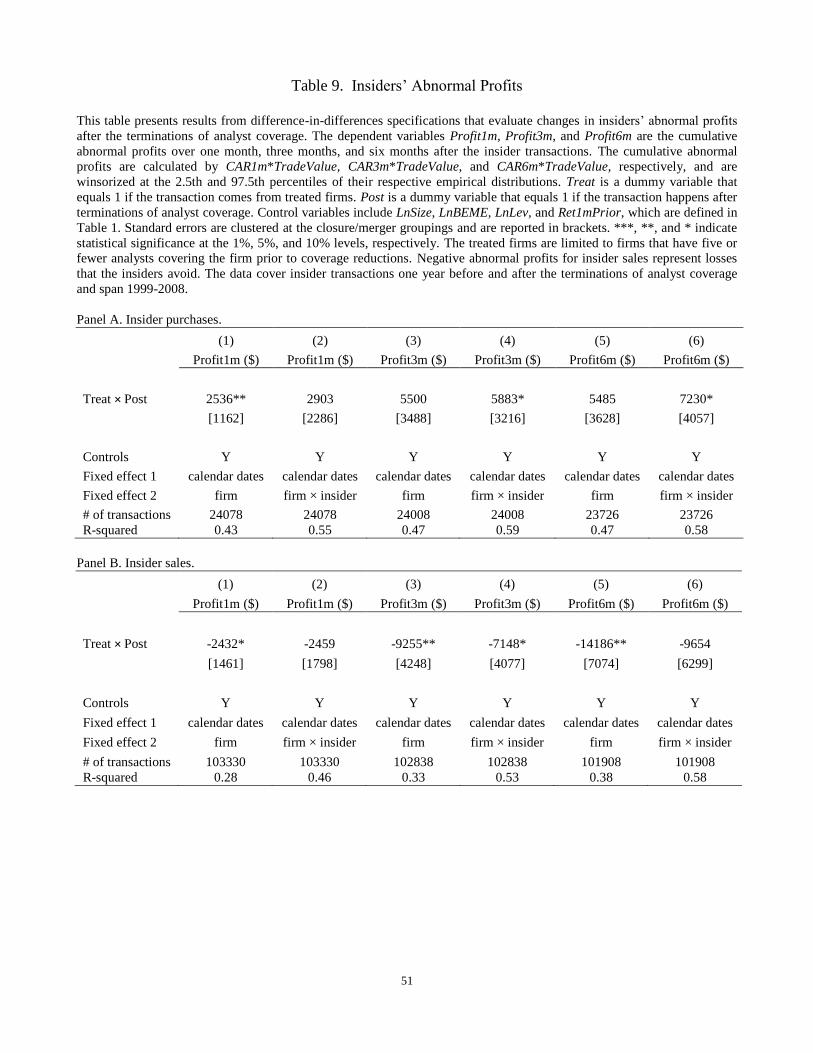
51
Table 9. Insiders’ Abnormal Profits
This table presents results from difference-in-differences specifications that evaluate changes in insiders’ abnormal profits
after the terminations of analyst coverage. The dependent variables Profit1m, Profit3m, and Profit6m are the cumulative
abnormal profits over one month, three months, and six months after the insider transactions. The cumulative abnormal
profits are calculated by CAR1m*TradeValue, CAR3m*TradeValue, and CAR6m*TradeValue, respectively, and are
winsorized at the 2.5th and 97.5th percentiles of their respective empirical distributions. Treat is a dummy variable that
equals 1 if the transaction comes from treated firms. Post is a dummy variable that equals 1 if the transaction happens after
terminations of analyst coverage. Control variables include LnSize, LnBEME, LnLev, and Ret1mPrior, which are defined in
Table 1. Standard errors are clustered at the closure/merger groupings and are reported in brackets. ***, **, and * indicate
statistical significance at the 1%, 5%, and 10% levels, respectively. The treated firms are limited to firms that have five or
fewer analysts covering the firm prior to coverage reductions. Negative abnormal profits for insider sales represent losses
that the insiders avoid. The data cover insider transactions one year before and after the terminations of analyst coverage
and span 1999-2008.
Panel A. Insider purchases.
(1) (2) (3) (4) (5) (6)
Profit1m ($) Profit1m ($) Profit3m ($) Profit3m ($) Profit6m ($) Profit6m ($)
Treat × Post 2536** 2903 5500 5883* 5485 7230*
[1162] [2286] [3488] [3216] [3628] [4057]
Controls Y Y Y Y Y Y
Fixed effect 1 calendar dates calendar dates calendar dates calendar dates calendar dates calendar dates
Fixed effect 2 firm firm × insider firm firm × insider firm firm × insider
# of transactions 24078 24078 24008 24008 23726 23726
R-squared 0.43 0.55 0.47 0.59 0.47 0.58
Panel B. Insider sales.
(1) (2) (3) (4) (5) (6)
Profit1m ($) Profit1m ($) Profit3m ($) Profit3m ($) Profit6m ($) Profit6m ($)
Treat × Post -2432* -2459 -9255** -7148* -14186** -9654
[1461] [1798] [4248] [4077] [7074] [6299]
Controls Y Y Y Y Y Y
Fixed effect 1 calendar dates calendar dates calendar dates calendar dates calendar dates calendar dates
Fixed effect 2 firm firm × insider firm firm × insider firm firm × insider
# of transactions 103330 103330 102838 102838 101908 101908
R-squared 0.28 0.46 0.33 0.53 0.38 0.58

52
Table 10. Aggregate Abnormal Profits
This table presents results from difference-in-differences specifications that evaluate changes in the aggregate abnormal
profits after the terminations of analyst coverage. The cumulative abnormal profits over one month, three months, and six
months after the insider transactions are aggregated at the insider-quarter level (IQ_Profit1m, IQ_Profit3m, and
IQ_Profit6m). The cumulative abnormal profits are winsorized at the 2.5th and 97.5th percentiles of their respective
empirical distributions. Treat is a dummy variable that equals 1 if the transaction comes from treated firms. Post is a
dummy variable that equals 1 if the transaction happens after the terminations of analyst coverage. Control variables
include LnSize, LnBEME, LnLev, and Ret1mPrior, which are defined in Table 1. Standard errors are clustered at the
closure/merger groupings and are reported in brackets. ***, **, and * indicate statistical significance at the 1%, 5%, and 10%
levels, respectively. The treated firms are limited to firms that have five or fewer analysts covering the firm prior to
coverage reductions. Negative abnormal profits for insider sales represent losses that the insiders avoid. The data cover
insider transactions one year before and after the terminations of analyst coverage and span 1999-2008.
(1) (2) (3) (4) (5) (6)
Insider Purchases
Insider Sales
IQ_Profit1m
($)
IQ_Profit3m
($)
IQ_Profit6m
($)
IQ_Profit1m
($)
IQ_Profit3m
($)
IQ_Profit6m
($)
Treat × Post 4078 14914* 21861***
-32953** -133325*** -224229***
[3133] [6805] [5390]
[12822] [41643] [74546]
Controls Y Y Y
Y Y Y
Fixed effect 1 year year year
year year year
Fixed effect 2 firm × insider firm × insider firm × insider
firm × insider firm × insider firm × insider
# of insider-quarters 6824 6824 6824
14288 14288 14288
R-squared 0.27 0.27 0.30 0.18 0.22 0.27
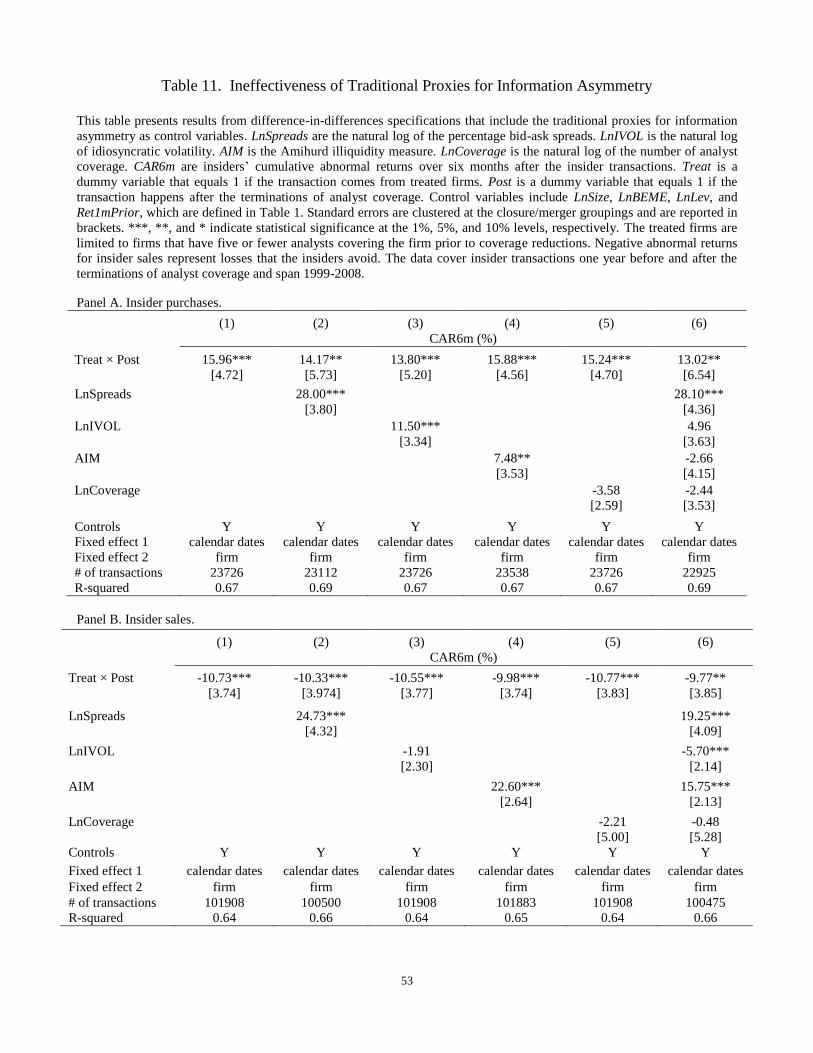
53
Table 11. Ineffectiveness of Traditional Proxies for Information Asymmetry
This table presents results from difference-in-differences specifications that include the traditional proxies for information
asymmetry as control variables. LnSpreads are the natural log of the percentage bid-ask spreads. LnIVOL is the natural log
of idiosyncratic volatility. AIM is the Amihurd illiquidity measure. LnCoverage is the natural log of the number of analyst
coverage. CAR6m are insiders’ cumulative abnormal returns over six months after the insider transactions. Treat is a
dummy variable that equals 1 if the transaction comes from treated firms. Post is a dummy variable that equals 1 if the
transaction happens after the terminations of analyst coverage. Control variables include LnSize, LnBEME, LnLev, and
Ret1mPrior, which are defined in Table 1. Standard errors are clustered at the closure/merger groupings and are reported in
brackets. ***, **, and * indicate statistical significance at the 1%, 5%, and 10% levels, respectively. The treated firms are
limited to firms that have five or fewer analysts covering the firm prior to coverage reductions. Negative abnormal returns
for insider sales represent losses that the insiders avoid. The data cover insider transactions one year before and after the
terminations of analyst coverage and span 1999-2008.
Panel A. Insider purchases.
(1) (2) (3) (4) (5) (6)
CAR6m (%)
Treat × Post 15.96*** 14.17** 13.80*** 15.88*** 15.24*** 13.02**
[4.72] [5.73] [5.20] [4.56] [4.70] [6.54]
LnSpreads
28.00***
28.10***
[3.80]
[4.36]
LnIVOL
11.50***
4.96
[3.34]
[3.63]
AIM
7.48**
-2.66
[3.53]
[4.15]
LnCoverage
-3.58 -2.44
[2.59] [3.53]
Controls Y Y Y Y Y Y
Fixed effect 1 calendar dates calendar dates calendar dates calendar dates calendar dates calendar dates
Fixed effect 2 firm firm firm firm firm firm
# of transactions 23726 23112 23726 23538 23726 22925
R-squared 0.67 0.69 0.67 0.67 0.67 0.69
Panel B. Insider sales.
(1) (2) (3) (4) (5) (6)
CAR6m (%)
Treat × Post -10.73*** -10.33*** -10.55*** -9.98*** -10.77*** -9.77**
[3.74] [3.974] [3.77] [3.74] [3.83] [3.85]
LnSpreads
24.73***
19.25***
[4.32]
[4.09]
LnIVOL
-1.91
-5.70***
[2.30]
[2.14]
AIM
22.60***
15.75***
[2.64]
[2.13]
LnCoverage
-2.21 -0.48
[5.00] [5.28]
Controls Y Y Y Y Y Y
Fixed effect 1 calendar dates calendar dates calendar dates calendar dates calendar dates calendar dates
Fixed effect 2 firm firm firm firm firm firm
# of transactions 101908 100500 101908 101883 101908 100475
R-squared 0.64 0.66 0.64 0.65 0.64 0.66
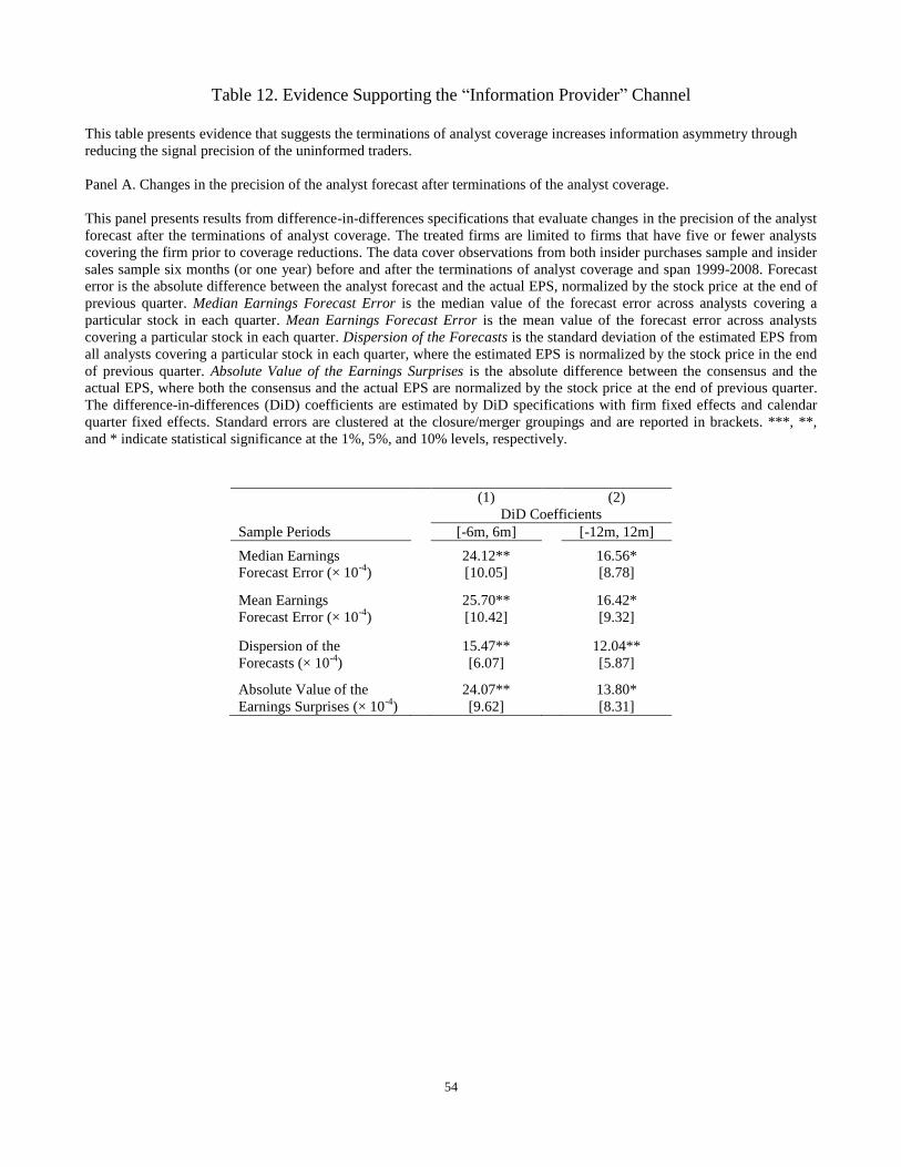
54
Table 12. Evidence Supporting the “Information Provider” Channel
This table presents evidence that suggests the terminations of analyst coverage increases information asymmetry through
reducing the signal precision of the uninformed traders.
Panel A. Changes in the precision of the analyst forecast after terminations of the analyst coverage.
This panel presents results from difference-in-differences specifications that evaluate changes in the precision of the analyst
forecast after the terminations of analyst coverage. The treated firms are limited to firms that have five or fewer analysts
covering the firm prior to coverage reductions. The data cover observations from both insider purchases sample and insider
sales sample six months (or one year) before and after the terminations of analyst coverage and span 1999-2008. Forecast
error is the absolute difference between the analyst forecast and the actual EPS, normalized by the stock price at the end of
previous quarter. Median Earnings Forecast Error is the median value of the forecast error across analysts covering a
particular stock in each quarter. Mean Earnings Forecast Error is the mean value of the forecast error across analysts
covering a particular stock in each quarter. Dispersion of the Forecasts is the standard deviation of the estimated EPS from
all analysts covering a particular stock in each quarter, where the estimated EPS is normalized by the stock price in the end
of previous quarter. Absolute Value of the Earnings Surprises is the absolute difference between the consensus and the
actual EPS, where both the consensus and the actual EPS are normalized by the stock price at the end of previous quarter.
The difference-in-differences (DiD) coefficients are estimated by DiD specifications with firm fixed effects and calendar
quarter fixed effects. Standard errors are clustered at the closure/merger groupings and are reported in brackets. ***, **,
and * indicate statistical significance at the 1%, 5%, and 10% levels, respectively.
(1)
(2)
DiD Coefficients
Sample Periods [-6m, 6m] [-12m, 12m]
Median Earnings
24.12**
16.56*
Forecast Error (× 10-4
)
[10.05]
[8.78]
Mean Earnings
25.70**
16.42*
Forecast Error (× 10-4
)
[10.42]
[9.32]
Dispersion of the
15.47**
12.04**
Forecasts (× 10-4
)
[6.07]
[5.87]
Absolute Value of the
24.07**
13.80*
Earnings Surprises (× 10-4
) [9.62] [8.31]

55
Table 12. Evidence supporting the “Information Provider” Channel (continued)
Panel B. Heterogeneity across the reduction in the precision of the analyst forecasts.
This panel presents results from difference-in-differences specifications that illustrate the heterogeneity in the treatment
effects across the level of reduction in the precision of the analyst forecasts. CAR6m are insiders’ cumulative abnormal
returns over six months after the insider transactions. Treat is a dummy variable that equals 1 if the transaction comes from
treated firms. Post is a dummy variable that equals 1 if the transaction happens after the terminations of analyst coverage.
Treated firms are sorted into two groups based on the level of reduction in the precision of the analyst forecasts. I compute
the first principle component (PCA1) of the four measures of the precision of the analyst forecasts: Median Earnings
Forecast Error, Mean Earnings Forecast Error, Dispersion of the Forecasts, and Absolute Value of the Earnings Surprises.
I then sort the treated firms into two bins based on the level of reduction in the precision of the analyst forecasts (i.e., the
average PCA1 one year after the terminations of analyst coverage minus the average PCA1 one year before the terminations
of analyst coverage). I perform the sorting annually and independently of the number of analysts prior to the coverage
reductions to ensure the two groups of firms have the same treatment intensity. High_Precision_Reduction is a dummy
variable that equals 1 if a firm’s reduction in the precision of the analyst forecast is larger than the median values. Control
variables include LnSize, LnBEME, LnLev, and Ret1mPrior which are defined in Table 1. Standard errors are clustered at
the closure/merger groupings and are reported in brackets. ***, **, and * indicate statistical significance at the 1%, 5%, and
10% levels, respectively. The treated firms are limited to firms that have five or fewer analysts covering the firm prior to
coverage reductions. Negative abnormal returns for insider sales represent losses that the insiders avoid. The data cover
insider transactions one year before and after the terminations of analyst coverage and span 1999-2008.
(1) (2) (3) (4)
Insider Purchases
Insider Sales
CAR6m (%) CAR6m (%)
CAR6m (%) CAR6m (%)
Treat × Post 7.17* 12.26*
-4.70 -3.94
[3.70] [6.55]
[3.90] [4.22]
Treat × Post × 12.55** 10.80*
-24.59** -24.83**
High_Precision_Reduction [5.01] [5.64]
[11.49] [11.19]
Controls Y Y
Y Y
Fixed effect 1 calendar dates calendar dates
calendar dates calendar dates
Fixed effect 2 firm firm × insider
firm firm × insider
# of observations 20220 20220
99020 99020
R-squared 0.68 0.83 0.64 0.78

56
Table 13. Evidence against the “Discipline” Channel as the Sole Explanation
This table presents results from specifications that evaluate changes in the performance of active mutual funds in trading
the affected stocks around the terminations of analyst coverage. For every stock that experiences coverage reductions, an
aggregate mutual fund is constructed by aggregating the holdings of all the active funds that hold this stock in the one-year
window prior to the terminations. Active funds include transient and dedicated investors following the classification
methods in Bushee (1998). The quarterly “trading” directions ( ) of this aggregate fund are then determined based on the
weights of the affected stock calculated from the quarterly holdings data. = 1 (or -1) if the weights of the affected
stocks increase (or decrease) after adjusting for the price changes of all the stocks in the aggregated fund. The dependent
variables are the excess returns of the aggregate mutual funds calculated by subtracting the returns of the characteristic-
based benchmarks (Daniel et al. 1997, Wermers 2004) from the raw returns of the affected stocks. Post is a dummy variable
that equals 1 for quarters after the terminations of analyst coverage. I include the excess returns four quarters before and
after the termination dates in the regression. Standard errors are clustered at the closure/merger groupings and are reported
in brackets. ***, **, and * indicate statistical significance at the 1%, 5%, and 10% levels, respectively.
(1) (2) (3)
All Sample
Increased Holdings Decreased Holdings
Sample ( = ±1)
( = 1) ( = -1)
Quarterly Abnormal Returns for the Active Mutual Funds (%)
Post 1.18**
1.86*** 0.40
[0.57]
[0.48] [0.66]
Fixed effect 1 year
year year
Fixed effect 2 fund
fund fund
# of fund-quarters 5526
2533 2993
R-squared 0.31 0.82 0.76
i
Internet Appendix
A. Additional Heterogeneity Tests
A.1 Heterogeneity across Insiders’ Trading Patterns
Corporate insiders trade for a variety of reasons. On one hand, they may trade on their private
information to gain abnormal profits. On the other hand, personal liquidity, diversification, signaling,
and other motivations that are not necessarily information driven can drive their transactions. Cohen,
Malloy, and Pomorski (2012) sort corporate insiders into “routine” traders and “opportunistic” traders
based on their trading patterns. They find that “opportunistic” traders earn significant abnormal
returns, whereas the returns for “routine” traders are essentially zero. Because “opportunistic” traders
are more likely to be the insiders who trade actively on their private information, I expect them to be
more aggressive in taking advantage of the increased information asymmetry after terminations of
analyst coverage. To test this hypothesis, I follow Cohen, Malloy, and Pomorski (2012) and identify
the insiders’ type based on their historical trading patterns. Specifically, I define insiders as routine
traders if they place a trade in the same calendar month in the three-year window prior to the
terminations of analyst coverage. I define opportunistic traders as everyone else. Because the
terminations of analyst coverage happen at the firm level, I compute the concentration of opportunistic
traders at the firm level and then sort all the treated firms into two groups based on this measure. I
perform the sorting annually and independently of the number of analysts to ensure the two groups of
firms have the same treatment intensity. I create a dummy variable High_Pct_Opportunistic_Insider
that equals 1 if a firm’s concentration of opportunistic traders is larger than the median values. I then
interact this dummy variable with the DiD term and run the following regression:
Here, represents the change in insiders’ abnormal returns for firms populated with routine
insiders. represents the additional treatment effects for firms populated with opportunistic insiders. I
do not include the dummy variable High_Pct_Opportunistic_Insider in the regression, because I have
already included firm fixed effects in the regression. Table A2 presents the results of the regressions.
For firms populated with routine insiders, the changes in insiders’ abnormal returns after terminations
of analyst coverage are essentially zero. The treatment effects come from firms populated with
opportunistic insiders. These results suggest that in order to earn abnormal profits, insiders who exhibit
opportunistic trading behaviors actively trade on the increased informational advantage brought by the
coverage reductions.
A.2 Heterogeneity across Insiders’ Diversification Need
Insiders’ stockholdings of their own companies can be a non-trivial portion of their wealth,
because they are commonly compensated with stocks and options. Thus, insiders’ desire to diversify
may affect their incentives to take advantage of the increased information asymmetry after coverage
reductions. Insiders who have a higher level of firm stockholdings are probably more likely to sell and
less likely to purchase when information asymmetry increases. To test this hypothesis, I use
ExecuComp data to compute the percentage of stocks and options in insiders’ total compensations in
ii
the three-year time window prior to the terminations of analyst coverage. I define insiders as
incentivized insiders if more than 75% of their compensation is paid using stocks and options.1 I then
compute the concentration of incentivized insiders at the firm level and sort the treated firms into two
groups based on this measure. I perform the sorting annually and independently of the number of
analysts to ensure the two groups of firms have the same treatment intensity. I create a dummy variable
High_Pct_Incentivized_Insider that equals 1 if a firm’s concentration of incentivized insiders is larger
than the median values. I then interact this dummy variable with the DiD term and run the following
regression:
Table A3 presents the results of the regressions. In the insider purchases sample, the DiD
coefficients are significantly positive for firms populated with non-incentivized insiders. However, the
treatment effects are much weaker and are essentially zero for firms populated with incentivized
insiders, suggesting that insiders who have heavy exposure to the stocks of their own companies avoid
purchasing additional stocks when information asymmetry increases. The results in the insider sales
sample are the opposite. All the treatment effects come from firms populated with incentivized insiders
in the insider sales sample, suggesting that insiders who have heavy exposure to the stocks of their own
companies actively sell their stocks when information asymmetry increases. The above results confirm
the hypothesis that insiders’ desire to diversify influences their response to changes in information
asymmetry.
A.3 Heterogeneity across Intensity of Regulatory Enforcement
If insiders trade on their private information to gain abnormal profits, they should be concerned
about the potential litigation risks and adjust their trading behavior according to the intensity of legal
enforcement. Del Guercio, Odders-White, and Ready (2013) show that the SEC enforcement intensity
deters illegal insider trading. Cohen, Malloy, and Pomorski (2012) show that opportunistic corporate
insiders reduce their trades followings waves of the SEC insider trading enforcement. In the context of
my paper, insiders should be less aggressive in taking advantage of the increased information
asymmetry during time periods with a higher intensity of legal enforcement. To test this hypothesis, I
sort calendar months into two bins based on the number of litigation cases released by the SEC. I
perform the sorting annually to remove any time trend in the SEC enforcement activities. I use the one-
month-lagged number under the assumption that insiders adjust their behavior after observing the
enforcement activities of the SEC in the previous month. I create a dummy variable
Low_Enforcement_Intensity that equals 1 if insider transactions take place in the calendar month with
low enforcement intensity. I then interact this dummy variable with the DiD term and run the
following regression:
Here, represents the change in insiders’ abnormal returns during time periods with a high
intensity of legal enforcement. represents the additional treatment effects during time periods with
1 Results are robust to other cutoffs, such as 50% and 90%.
iii
a low intensity of legal enforcement. Notice that I do not include the dummy variable
Low_Enforcement_Intensity itself in the regression, because I have already included time fixed effects
in the regression. Table A4 presents the results of the regressions. In time periods with a high intensity
of legal enforcement, the changes in insiders’ abnormal returns after terminations of analyst coverage
are not statistically significant. However, in both insider transaction samples, the treatment effects are
significantly stronger in time periods with a low intensity of legal enforcement. These results suggest
that litigation risks can deter insiders from taking advantage of the increase in information asymmetry
after terminations of analyst coverage.
B. Additional Robustness Tests
B.1 Alternative Measures of Abnormal Returns
The abnormal returns used in the baseline specifications are cumulative abnormal returns
(CARs). CARs ignore compounding, because they use arithmetic rather than geometric averages. Thus,
CARs do not represent realized returns from an investor’s point of view. Buy-and-hold abnormal
returns (BHARs) are the alternative measure for abnormal returns. BHARs are the compound returns
from a sample firm less the compound returns from a reference portfolio. Table A5 presents the
coefficients in the DiD analysis using BHARs with the Fama-French 25 portfolio returns as the
reference portfolio.2 In the insider purchases sample, the six-month BHARs increase significantly after
the terminations of analyst coverage. The DiD coefficients have a similar magnitude to those in the
baseline analysis using CARs. In the insider sales sample, the coefficients are negative. However, their
magnitude is significantly smaller compared to those from the baseline analysis. This difference is
probably due to severe positive skewness, a prominent drawback of BHARs (Barber and Lyon 1997).
In contrast to cumulative returns, compound buy-and-hold returns have lower bounds at -100%.
Moreover, the returns of the individual stocks are more volatile compared to the returns of the
reference portfolio in most cases. For example, it is common to observe a sample firm with an annual
return in excess of 100%, but rare to observe a return on a Fama-French 25 portfolio in excess of 100%.
Because BHARs are calculated as the compound sample firm return less the compound Fama-French
25 portfolio return, they are positively skewed. Therefore, we naturally have limited room to observe
the negative shifts in BHARs after the terminations of analyst coverage. Whether CARs or BHARs are
more appropriate for evaluating abnormal returns is still a topic up for debate in the literature. In the
context of my paper, if we assume no portfolio rebalancing and calculate the gain or loss for those
insiders within the sample, BHARs are perhaps better choices conceptually. However, if we are more
interested in investigating the impact of information asymmetry on price efficiency, or assessing the
profits for informed traders in a broader sense (e.g., insiders who can rebalance their portfolios), CARs
probably constitute a better choice.
B.2 Control for Liquidity Measures
One potential concern about the analysis is that the terminations of analyst coverage will
change stock liquidity, which in turn affects the stock returns. I acknowledge this possibility but would
like to point out that the change in liquidity itself can be a consequence of an increase in information
asymmetry (Kelly and Ljungqvist 2012, Vayanos and Wang 2011). Therefore, the ideal approach is to
2
, where is the return of the individual firms and is the return of the
corresponding Fama-French 25 portfolio.
iv
separate out the component of stock liquidity that is orthogonal to the change in information
asymmetry, and then add it to the DiD specifications as a control. However, empirically this approach
is extremely challenging, if not impossible. As a step toward this goal, I add two liquidity measures as
additional controls in the analysis. The first measure is the Amihud illiquidity measure (Amihud 2002),
which is the ratio of the absolute return to the dollar volume of trading. The second measure is
historical liquidity beta (Pastor and Stambaugh 2003), which reflects firms’ sensitivity to changes in
aggregate liquidity. Table A6 presents the regression results after adding these two liquidity measures
as additional controls. Consistent with previous literature, both the Amihud illiquidity measure and
historical liquidity beta are positively correlated with expected stock returns (Amihud 2002; Chordia,
Huh, and Subrahmanyam 2009; Pastor and Stambaugh 2003). The coefficients of the DiD terms
remain positive in the insider purchases sample and negative in the insider sales sample, with
magnitudes similar to those in the baseline analysis. Note that the coefficients of the DiD terms in
Table A6 may still be biased because the liquidity measures contain signals of information asymmetry.
However, given that I obtain similar coefficients in the specifications with and without liquidity
measures, controlling for the liquidity component that is orthogonal to information asymmetry is
unlikely to overturn the results in the baseline analysis.
B.3 Exclude Tiny Firms and Low-price Transactions
As the summary statistics show, the firm size in my sample is relatively small, which raises a
concern that tiny firms are the primary driver of the treatment results, which, if true, would cast doubts
on the external validity of my analysis. To rule out this possibility, I first exclude all firms smaller than
100M, and then re-run the DiD analysis. The resulting data set contains 78.2% of the purchases and
92.4% of the sales in the baseline analysis. Panel A of Table A7 presents the regression results. The
coefficients of the DiD terms remain similar to those in the baseline specifications. Next, I further
exclude insider transactions with prices less than $5. The resulting data set contains 62.6% of the
purchases and 89.4% of the sales in the baseline analysis. Panel B of Table A7 shows the regression
results for insiders’ abnormal returns. Again, the coefficients of the DiD terms are similar to those in
the baseline specifications. Taken together, these results suggest the treatment effects that I find in the
baseline analysis are not limited to tiny firms or low-price transactions.
B.4 Placebo Tests
Two pieces of information associated with the coverage reductions are essential for the DiD
analysis: which firms receive the coverage reductions (identified by PERMNOs) and when the
coverage reductions occur (termination dates). I falsely replace these two pieces of information one at
a time to generate “placebo termination” and then re-run the analysis. In the first placebo test, I falsely
shift termination dates backward for three years, while keeping the identities of the treated firms
unchanged. In the second test, I falsely replace treated firms with control firms that are in the same
Fama-French size and book-to-market quintile and have close bid-ask spreads, while keeping the
termination dates unchanged. Panel A and Panel B of Table A8 present the regression results of the
above two placebo tests, respectively. The coefficients of the Treat × Post terms are no longer
significant in either of these two tests, suggesting the treatment effects I find in the baseline analysis
are not driven by the identities of the treated firms or the termination dates alone, but rather by the
combination of the two (i.e., the actual terminations of analyst coverage).
C. Changes in Insiders’ Trading Probability

v
Does the increase in information asymmetry alter insiders’ trading behavior in the extensive
margin? To address this question, I examine whether the probability of insider trading changes in
response to an increase in information asymmetry. I construct a firm-day panel containing all trading
dates one year before and after the terminations of analyst coverage for every firm in my sample. The
dependent variable Buy (Sell) is a dummy variable that equals 1 if insiders purchase (sell) in a given
firm-day. The mean value of Buy is 3.5% (i.e., insiders in a given firm buy in one day out of every 29
trading days), whereas the mean value of Sell is 6.2% (i.e., insiders in a given firm sell in one day out
of every 16 trading days). I run the DiD analysis using linear probability models. Table A9 presents the
coefficients of the tests.
Consistent with previous studies (Rozeff and Zaman 1998, Lakonishok and Lee 2001, Jenter
2005), I find that insiders try to time the market when they trade. First, insiders appear to exploit the
size premium. The coefficients of LnSize are significantly negative for insider purchases and
significantly positive for insider sales, which indicates insiders are more likely to buy when firm size
decreases and more likely to sell when firm size increases. Second, insiders also exploit the value
premium. The coefficients of LnBEME are significantly negative for insider sales, suggesting insiders
are less likely to sell when the book-to-market ratio increases. Furthermore, insiders bet heavily on
short-term reversals. The coefficients of Ret1mPrior are significantly negative for insider purchases
and significantly positive for insider sales, which means insiders are more likely to buy when stock
price has recently decreased and more likely to sell when stock price has recently increased.
Similar to the trading volume, the increase in information asymmetry also alters insiders’
trading probability in a way that depends on the liquidity of the stocks. For stocks with high liquidity
(quartile 1 sorted by the bid-ask spreads), the trading probability increases significantly by 1.8% in the
insider purchases sample, and by 4.0% (both in absolute terms) in the insider sales sample, whereas the
trading probability remains the same for other stocks (quartile 2, 3, and 4 sorted by the bid-ask
spreads). These results suggest information asymmetry also influences insiders’ trading behavior in the
extensive margin.
References:
Amihud, Yakov, 2002, Illiquidity and Stock Returns: Cross-section and Time-series Effects, Journal of
Financial Markets 5, 31–56.
Barber, Brad M, and John D Lyon, 1997, Detecting Long-run Abnormal Stock Returns: The Empirical
Power and Specification of Test Statistics, Journal of Financial Economics 43, 341–372.
Chordia, Tarun, Sahn-Wook Huh, and Avanidhar Subrahmanyam, 2009, Theory-Based Illiquidity and
Asset Pricing, Review of Financial Studies 22, 3629–3668.
Cohen, Lauren, Christopher Malloy, and Lukasz Pomorski, 2012, Decoding Inside Information,
Journal of Finance 67, 1009–1043.

vi
Del Guercio, Diane, Elizabeth R. Odders-White, and Mark J. Ready, 2013. The Deterrence effect of
SEC enforcement intensity on illegal insider trading, working paper.
Jenter, Dirk, 2005, Market Timing and Managerial Portfolio Decisions, Journal of Finance 60, 1903–
1949.
Kelly, B., and a. Ljungqvist, 2012, Testing Asymmetric-Information Asset Pricing Models, Review of
Financial Studies 25, 1366–1413.
Lakonishok, Josef, and Inmoo Lee, 2001, Are Insider Trades Informative?, Review of Financial
Studies 14, 79–111.
Pastor, Lubos, and Robert F Stambaugh, 2003, Liquidity risk and expected stock returns, Journal of
Political Economy 111, 642–685.
Rozeff, Michael S, and Mir A Zaman, 1998, Overreaction and Insider Trading: Evidence from Growth
and Value Portfolios, Journal of Finance 53, 701–716.
Vayanos, Dimitri, and Jiang Wang, 2011, Liquidity and Asset Returns Under Asymmetric Information
and Imperfect Competition, Review of Financial Studies 25, 1339–1365.

vii
Table A1. Impact of the Sarbanes-Oxley (SOX) Act
This table presents results from difference-in-differences specifications that evaluate the impact of the SOX Act on the
changes in insiders’ abnormal returns after the terminations of analyst coverage. SOX is a dummy variable that equals 1 if
the transaction happens in September, 2003 or after. CAR6m are insiders’ cumulative abnormal returns over six months
after the insider transactions. CARTtoF are insiders’ cumulative abnormal returns from the trading dates to the filing dates.
CARFto6m are insiders’ cumulative abnormal returns from the filing dates to six months after the trading dates. Treat is a
dummy variable that equals 1 if the transaction comes from treated firms. Post is a dummy variable that equals 1 if the
transaction happens after the terminations of analyst coverage. Control variables include LnSize, LnBEME, LnLev, and
Ret1mPrior, which are defined in Table 1. Standard errors are clustered at the closure/merger groupings and are reported in
brackets. ***, **, and * indicate statistical significance at the 1%, 5%, and 10% levels, respectively. The treated firms are
limited to firms that have five or fewer analysts covering the firm prior to coverage reductions. Negative abnormal returns
for insider sales represent losses that the insiders avoid. The data cover insider transactions one year before and after the
terminations of analyst coverage and span 1999-2008.
(1) (2) (3) (4) (5) (6)
Insider Purchases
Insider Sales
CAR6m (%) CARTtoF (%) CARFto6m (%)
CAR6m (%) CARTtoF (%) CARFto6m (%)
Treat × Post 16.92*** 3.70* 12.39*
-12.59** -3.60*** -8.65**
[5.95] [2.05] [6.92]
[5.11] [1.33] [3.82]
Treat × Post × SOX
-6.10 -2.87 -1.81
3.41 3.76*** -0.24
[12.94] [2.31] [16.56]
[7.45] [1.45] [7.21]
Controls Y Y Y
Y Y Y
Fixed effect 1 calendar dates calendar dates calendar dates
calendar dates calendar dates calendar dates
Fixed effect 2 firm firm firm
firm firm firm
# of transactions 23726 20995 20980
101908 100499 100494
R-squared 0.67 0.52 0.69 0.64 0.41 0.64
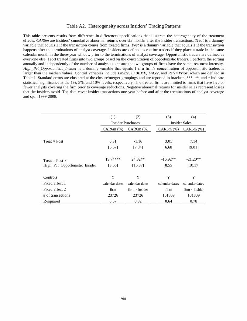
viii
Table A2. Heterogeneity across Insiders’ Trading Patterns
This table presents results from difference-in-differences specifications that illustrate the heterogeneity of the treatment
effects. CAR6m are insiders’ cumulative abnormal returns over six months after the insider transactions. Treat is a dummy
variable that equals 1 if the transaction comes from treated firms. Post is a dummy variable that equals 1 if the transaction
happens after the terminations of analyst coverage. Insiders are defined as routine traders if they place a trade in the same
calendar month in the three-year window prior to the terminations of analyst coverage. Opportunistic traders are defined as
everyone else. I sort treated firms into two groups based on the concentration of opportunistic traders. I perform the sorting
annually and independently of the number of analysts to ensure the two groups of firms have the same treatment intensity.
High_Pct_Opportunistic_Insider is a dummy variable that equals 1 if a firm’s concentration of opportunistic traders is
larger than the median values. Control variables include LnSize, LnBEME, LnLev, and Ret1mPrior, which are defined in
Table 1. Standard errors are clustered at the closure/merger groupings and are reported in brackets. ***, **, and * indicate
statistical significance at the 1%, 5%, and 10% levels, respectively. The treated firms are limited to firms that have five or
fewer analysts covering the firm prior to coverage reductions. Negative abnormal returns for insider sales represent losses
that the insiders avoid. The data cover insider transactions one year before and after the terminations of analyst coverage
and span 1999-2008.
(1) (2) (3) (4)
Insider Purchases
Insider Sales
CAR6m (%) CAR6m (%)
CAR6m (%) CAR6m (%)
Treat × Post 0.81 -1.16
3.01 7.14
[6.67] [7.84]
[6.68] [9.01]
Treat × Post ×
High_Pct_Opportunistic_Insider
19.74*** 24.82**
-16.92** -21.20**
[3.66] [10.37]
[8.55] [10.17]
Controls Y Y
Y Y
Fixed effect 1 calendar dates calendar dates
calendar dates calendar dates
Fixed effect 2 firm firm × insider
firm firm × insider
# of transactions 23726 23726
101809 101809
R-squared 0.67 0.82 0.64 0.78

ix
Table A3. Heterogeneity across Insiders’ Diversification Need
This table presents results from difference-in-differences specifications that illustrate the heterogeneity of the treatment
effects. CAR6m are insiders’ cumulative abnormal returns over six months after the insider transactions. Treat is a dummy
variable that equals 1 if the transaction comes from treated firms. Post is a dummy variable that equals 1 if the transaction
happens after the terminations of analyst coverage. Insiders are defined as incentivized insiders if more than 75% of their
total compensations are paid using stocks and options in the three-year time window prior to the terminations of analyst
coverage. I sort treated firms into two groups based on the concentration of incentivized traders. I perform sorting annually
and independently of the number of analysts to ensure the two groups of firms have the same treatment intensity.
High_Pct_ Incentivized_Insider is a dummy variable that equals 1 if a firm’s concentration of incentivized insiders is larger
than the median values. Control variables include LnSize, LnBEME, LnLev, and Ret1mPrior, which are defined in Table 1.
Standard errors are clustered at the closure/merger groupings and are reported in brackets. ***, **, and * indicate statistical
significance at the 1%, 5%, and 10% levels, respectively. The treated firms are limited to firms that have five or fewer
analysts covering the firm prior to coverage reductions. Negative abnormal returns for insider sales represent losses that the
insiders avoid. The data cover insider transactions one year before and after the terminations of analyst coverage and span
1999-2008.
(1) (2) (3) (4)
Insider Purchases
Insider Sales
CAR6m (%) CAR6m (%)
CAR6m (%) CAR6m (%)
Treat × Post 19.69** 25.46**
-5.72 -9.27
[10.16] [12.09]
[5.16] [6.34]
Treat × Post ×
High_Pct_Incentivized_Insider
-16.14 -27.29**
-32.28*** -22.23***
[12.42] [13.70]
[10.45] [8.48]
Controls Y Y
Y Y
Fixed effect 1 calendar dates calendar dates
calendar dates calendar dates
Fixed effect 2 firm firm × insider
firm firm × insider
# of transactions 9586 9586
55026 55026
R-squared 0.78 0.90 0.63 0.79

x
Table A4. Heterogeneity across Intensity of Regulatory Enforcement
This table presents results from difference-in-differences specifications that illustrate the heterogeneity of the treatment
effects. CAR6m are insiders’ cumulative abnormal returns over six months after the insider transactions. Treat is a dummy
variable that equals 1 if the transaction comes from treated firms. Post is a dummy variable that equals 1 if the transaction
happens after the terminations of analyst coverage. I sort calendar months into two bins based on the number of litigation
cases released by the SEC. I perform the sorting annually to remove any time trend in the SEC enforcement activities. One-
month-lagged numbers are used in the sorting with the assumption that insiders adjust their trading behavior after observing
the enforcement activities of the SEC in the previous months. Low_Enforcement_Intensity is a dummy variable that equals
1 if insider transactions take place in the calendar month with low enforcement intensity. Control variables include LnSize,
LnBEME, LnLev, and Ret1mPrior, which are defined in Table 1. Standard errors are clustered at the closure/merger
groupings and are reported in brackets. ***, **, and * indicate statistical significance at the 1%, 5%, and 10% levels,
respectively. The treated firms are limited to firms that have five or fewer analysts covering the firm prior to coverage
reductions. Negative abnormal returns for insider sales represent losses that the insiders avoid. The data cover insider
transactions one year before and after the terminations of analyst coverage and span 1999-2008.
(1) (2) (3) (4)
Insider Purchases
Insider Sales
CAR6m (%) CAR6m (%)
CAR6m (%) CAR6m (%)
Treat × Post 5.05 11.38
1.86 -2.56
[8.47] [9.69]
[9.95] [9.06]
Treat × Post ×
Low_Enforcement_Intensity
18.45*** 16.06**
-15.01** -15.76***
[6.65] [6.94]
[6.76] [5.76]
Controls Y Y
Y Y
Fixed effect 1 calendar dates calendar dates
calendar dates calendar dates
Fixed effect 2 firm firm × insider
firm firm × insider
# of transactions 11631 11631
69908 69908
R-squared 0.71 0.82 0.64 0.78

xi
Table A5. Buy-and-Hold Abnormal Returns
This table presents results from difference-in-differences specifications that evaluate changes in insiders’ abnormal returns
after the terminations of analyst coverage, using an alternative measure. BHAR6m are insiders’ buy-and-hold abnormal
returns over six months after the insider transactions. BHAR6m are the compound returns on the individual firms less the
compound returns on the corresponding Fama-French 25 portfolio. Treat is a dummy variable that equals 1 if the
transaction comes from treated firms. Post is a dummy variable that equals 1 if the transaction happens after terminations of
analyst coverage. Control variables include LnSize, LnBEME, LnLev, and Ret1mPrior, which are defined in Table 1.
Standard errors are clustered at the closure/merger groupings and are reported in brackets. ***, **, and * indicate statistical
significance at the 1%, 5%, and 10% levels, respectively. The treated firms are limited to firms that have five or fewer
analysts covering the firm prior to coverage reductions. Negative abnormal returns for insider sales represent losses that the
insiders avoid. The data cover insider transactions one year before and after the terminations of analyst coverage and span
1999-2008.
(1) (2) (3) (4)
Insider Purchases
Insider Sales
BHAR6m (%) BHAR6m (%)
BHAR6m (%) BHAR6m (%)
Treat × Post 16.58*** 14.42***
-3.79* -4.91*
[3.79] [4.48]
[2.26] [2.62]
Controls Y Y
Y Y
Fixed effect 1 calendar dates calendar dates
calendar dates calendar dates
Fixed effect 2 firm firm × insider
firm firm × insider
# of transactions 23802 23802
103246 103246
R-squared 0.70 0.86 0.63 0.76

xii
Table A6. Control for Liquidity Measures
This table presents results from difference-in-differences specifications that evaluate changes in insiders’ abnormal returns
after the terminations of analyst coverage with liquidity measures as additional controls. AIM is the Amihud illiquidity
measure calculated by
(Amihud, 2002), and Liqbeta is the historical liquidity beta
(Pastor and Stambaugh, 2003). CAR6m are insiders’ cumulative abnormal returns over six months after the insider
transactions. Treat is a dummy variable that equals 1 if the transaction comes from treated firms. Post is a dummy variable
that equals 1 if the transaction happens after terminations of analyst coverage. Control variables include LnSize, LnBEME,
LnLev, and Ret1mPrior, which are defined in Table 1. Standard errors are clustered at the closure/merger groupings and are
reported in brackets. ***, **, and * indicate statistical significance at the 1%, 5%, and 10% levels, respectively. The treated
firms are limited to firms that have five or fewer analysts covering the firm prior to coverage reductions. Negative abnormal
returns for insider sales represent losses that the insiders avoid. The data cover insider transactions one year before and after
the terminations of analyst coverage and span 1999-2008.
(1) (2) (3) (4)
Insider Purchases
Insider Sales
CAR6m (%) CAR6m (%)
CAR6m (%) CAR6m (%)
Treat × Post 16.27*** 16.39***
-8.85** -9.38**
[4.39] [4.15]
[3.56] [3.87]
AIM 0.79 0.63
2.27** 1.91**
[0.84] [0.42]
[1.09] [0.95]
Liqbeta 41.25** 42.10**
12.43* 12.03
[18.21] [19.53]
[6.70] [7.51]
Controls Y Y
Y Y
Fixed effect 1 calendar dates calendar dates
calendar dates calendar dates
Fixed effect 2 firm firm × insider
firm firm × insider
# of transactions 16990 16990
75810 75810
R-squared 0.67 0.82 0.68 0.81
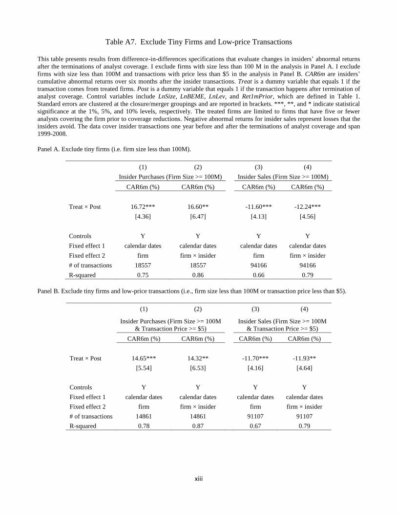
xiii
Table A7. Exclude Tiny Firms and Low-price Transactions
This table presents results from difference-in-differences specifications that evaluate changes in insiders’ abnormal returns
after the terminations of analyst coverage. I exclude firms with size less than 100 M in the analysis in Panel A. I exclude
firms with size less than 100M and transactions with price less than $5 in the analysis in Panel B. CAR6m are insiders’
cumulative abnormal returns over six months after the insider transactions. Treat is a dummy variable that equals 1 if the
transaction comes from treated firms. Post is a dummy variable that equals 1 if the transaction happens after termination of
analyst coverage. Control variables include LnSize, LnBEME, LnLev, and Ret1mPrior, which are defined in Table 1.
Standard errors are clustered at the closure/merger groupings and are reported in brackets. ***, **, and * indicate statistical
significance at the 1%, 5%, and 10% levels, respectively. The treated firms are limited to firms that have five or fewer
analysts covering the firm prior to coverage reductions. Negative abnormal returns for insider sales represent losses that the
insiders avoid. The data cover insider transactions one year before and after the terminations of analyst coverage and span
1999-2008.
Panel A. Exclude tiny firms (i.e. firm size less than 100M).
(1) (2) (3) (4)
Insider Purchases (Firm Size >= 100M)
Insider Sales (Firm Size >= 100M)
CAR6m (%) CAR6m (%)
CAR6m (%) CAR6m (%)
Treat × Post 16.72*** 16.60**
-11.60*** -12.24***
[4.36] [6.47]
[4.13] [4.56]
Controls Y Y
Y Y
Fixed effect 1 calendar dates calendar dates
calendar dates calendar dates
Fixed effect 2 firm firm × insider
firm firm × insider
# of transactions 18557 18557
94166 94166
R-squared 0.75 0.86 0.66 0.79
Panel B. Exclude tiny firms and low-price transactions (i.e., firm size less than 100M or transaction price less than $5).
(1) (2) (3) (4)
Insider Purchases (Firm Size >= 100M
& Transaction Price >= $5)
Insider Sales (Firm Size >= 100M
& Transaction Price >= $5)
CAR6m (%) CAR6m (%)
CAR6m (%) CAR6m (%)
Treat × Post 14.65*** 14.32**
-11.70*** -11.93**
[5.54] [6.53]
[4.16] [4.64]
Controls Y Y
Y Y
Fixed effect 1 calendar dates calendar dates
calendar dates calendar dates
Fixed effect 2 firm firm × insider
firm firm × insider
# of transactions 14861 14861
91107 91107
R-squared 0.78 0.87 0.67 0.79

xiv
Table A8. Placebo Tests
This table presents results from difference-in-differences specifications that evaluate changes in insiders’ abnormal returns
after the terminations of analyst coverage in two placebo tests. In Panel A, the treated firms remain the same as those in the
real test, but I shift the termination dates of the analyst coverage back for three years. In Panel B, the termination dates of
the analyst coverage remain the same as those in the real test, but I falsely replace the treated firms with a control firm that
has a similar bid-ask spread and is in the same Fama-French 25 portfolio. CAR6m are insiders’ cumulative abnormal returns
over six months after the insider transactions. Treat is a dummy variable that equals 1 if the transaction comes from treated
firms. Post is a dummy variable that equals 1 if the transaction happens after terminations of analyst coverage. Control
variables include LnSize, LnBEME, LnLev, and Ret1mPrior, which are defined in Table 1. Standard errors are clustered at
the closure/merger groupings and are reported in brackets. ***, **, and * indicate statistical significance at the 1%, 5%, and
10% levels, respectively. The treated firms are limited to firms that have five or fewer analysts covering the firm prior to
coverage reductions. Negative abnormal returns for insider sales represent losses that the insiders avoid. The data cover
insider transactions one year before and after the terminations of analyst coverage and span 1999-2008.
Panel A. Falsely shift termination dates back for three years.
(1) (2) (3) (4)
Insider Purchases
Insider Sales
CAR6m (%) CAR6m (%)
CAR6m (%) CAR6m (%)
Treat × Post -5.11 -7.39
2.13 -0.43
[6.90] [7.16]
[5.11] [5.48]
Controls Y Y
Y Y
Fixed effect 1 calendar dates calendar dates
calendar dates calendar dates
Fixed effect 2 firm firm × insider
firm firm × insider
# of transactions 9571 9571
35733 35733
R-squared 0.72 0.83 0.67 0.79
Panel B. Falsely replace treated firms with control firms in the same Fama-French 25 portfolio with close bid-ask spreads.
(1) (2) (3) (4)
Insider Purchases
Insider Sales
CAR6m (%) CAR6m (%)
CAR6m (%) CAR6m (%)
Treat × Post -13.10 -19.52
-0.49 0.39
[14.52] [19.71]
[5.92] [6.93]
Controls Y Y
Y Y
Fixed effect 1 calendar dates calendar dates
calendar dates calendar dates
Fixed effect 2 firm firm × insider
firm firm × insider
# of transactions 51031 51031
164610 164610
R-squared 0.60 0.73 0.56 0.71

xv
Table A9. Probability of Insider Trading
This table presents results from difference-in-differences specifications that evaluate changes in the probability of insider
trading after the terminations of analyst coverage. The dependent variable Buy (Sell) is a dummy variable that equals 1 if
insiders purchase (sell) in a given firm-day. Treat is a dummy variable that equals 1 if the transaction comes from treated
firms. Post is a dummy variable that equals 1 if the transaction happens after the terminations of analyst coverage. Treated
firms are sorted into quartiles based on the bid-ask spreads prior to the coverage reductions. I perform the sorting annually
and independently of the number of analysts to ensure the four groups of firms have the same treatment intensity. Firms in
Quartile 1 have the smallest bid-ask spreads and hence are the most liquid. SpreadQ12, SpreadQ34, SpreadQ1 and
SpreadQ234 are dummy variables that equal 1 if a firm’s average bid-ask spreads are in the corresponding quartile groups.
Control variables include LnSize, LnBEME, LnLev, and Ret1mPrior, which are defined in Table 1. Standard errors are
clustered at the closure/merger groupings and are reported in brackets. ***, **, and * indicate statistical significance at the
1%, 5%, and 10% levels, respectively. The treated firms are limited to firms that have five or fewer analysts covering the
firm prior to coverage reductions. The data are a full panel containing all firm-days one year before and after the
terminations of analyst coverage and span 1999-2008.
(1) (2) (3) (4) (5) (6)
Buy*100 (mean = 3.45)
Sell*100 (mean = 6.22)
Treat × Post 0.369
0.056
[0.352]
[0.560]
Treat × Post × SpreadQ12
0.786
1.047
[0.660]
[1.002]
Treat × Post × SpreadQ34
0.229
-0.112
[0.348]
[0.585]
Treat × Post × SpreadQ1
1.787***
3.990***
[0.619]
[0.505]
Treat × Post × SpreadQ234
0.176
-0.329
[0.352]
[0.628]
LnSize -0.421*** -0.418*** -0.420***
0.526*** 0.523*** 0.526***
[0.145] [0.143] [0.145]
[0.152] [0.150] [0.145]
LnBEME -0.339 -0.335 -0.337
-0.803*** -0.808*** -0.808***
[0.214] [0.213] [0.215]
[0.201] [0.201] [0.203]
LnLev 0.132 0.127 0.117
-0.609*** -0.614*** -0.613***
[0.231] [0.232] [0.235]
[0.158] [0.160] [0.159]
Ret1mPrior -0.041*** -0.040*** -0.040***
0.082*** 0.082*** 0.082***
[0.005] [0.005] [0.005]
[0.010] [0.010] [0.010]
Constant 5.476*** 5.464*** 5.478***
2.179** 2.193** 2.179**
[0.838] [0.834] [0.839]
[0.910] [0.905] [0.904]
# of firm-days 318926 318926 318926
479258 479258 479258
R-squared 0.003 0.003 0.003 0.007 0.007 0.007

xvi
Table A10. Characteristics of Prosecuted Illegal Insider Transactions
This table lists the abnormal returns and profits associated with the illegal insider trading cases reported by Meulbroek
(1992) and Del Guercio et al. (2013). Panel A lists the abnormal returns on the information announcement day. The
abnormal returns are estimated by regressions of daily returns on the market return, and dummies equal to 1 on the
information announcement day, insider trading day(s), and interim news day(s). Prior to calculating the statistics in Panel
A, the estimates from regressions for bad news events are multiplied by -1. Panel B lists the SEC-reported trading profits
for each trader in the illegal insider trading cases. Profits are either profits obtained or losses avoided as a result of the
illegal transactions, and they are converted to constant 2011 dollars.
Panel A: Information announcement day (e.g. takeovers) abnormal returns
Sample Period 1980-1989
2003-2007 & 2010-2011
Source Meulbroek (1992)
Del Guercio et al. (2013)
Mean 18.50%
22.75%
Median n/a
15.19%
Panel B: SEC-reported profits per trader ($ in Year 2011)
Sample Period 1980-1989 2003-2007 2010 - 2011
Source Meulbroek (1992) Del Guercio et al. (2013) Del Guercio et al. (2013)
Mean n/a
$519,116
$1,746,102
Median $55,722
$61,189
$177,297
![[CRISIL] Literature review on insider trading and insider ... · Literature review on Insider Trading and Insider Trading Regulation Abstract Views on insider trading and its effects](https://cdn.vdocument.in/doc/165x107/5ad077037f8b9a71028de0eb/crisil-literature-review-on-insider-trading-and-insider-review-on-insider.jpg)


