
Interpreting Assessments of Student Learning in the Introductory Physics Classroom and Laboratory
CitationDowd, Jason. 2012. Interpreting Assessments of Student Learning in the Introductory Physics Classroom and Laboratory. Doctoral dissertation, Harvard University.
Permanent linkhttp://nrs.harvard.edu/urn-3:HUL.InstRepos:9282889
Terms of UseThis article was downloaded from Harvard University’s DASH repository, and is made available under the terms and conditions applicable to Other Posted Material, as set forth at http://nrs.harvard.edu/urn-3:HUL.InstRepos:dash.current.terms-of-use#LAA
Share Your StoryThe Harvard community has made this article openly available.Please share how this access benefits you. Submit a story .
Accessibility

2012 - Jason Edward Dowd
All rights reserved.

iii
Dissertation Advisor: Professor Eric Mazur Jason Edward Dowd
Interpreting Assessments of Student Learning in the
Introductory Physics Classroom and Laboratory
Abstract
Assessment is the primary means of feedback between students and instructors. However, to
effectively use assessment, the ability to interpret collected information is essential. We present
insights into three unique, important avenues of assessment in the physics classroom and
laboratory.
First, we examine students’ performance on conceptual surveys. The goal of this research
project is to better utilize the information collected by instructors when they administer the Force
Concept Inventory (FCI) to students as a pre-test and post-test of their conceptual understanding
of Newtonian mechanics. We find that ambiguities in the use of the normalized gain, g, may
influence comparisons among individual classes. Therefore, we propose using stratagrams,
graphical summaries of the fraction of students who exhibit “Newtonian thinking,” as a clearer,
more informative method of both assessing a single class and comparing performance among
classes.
Next, we examine students’ expressions of confusion when they initially encounter new
material. The goal of this research project is to better understand what such confusion actually
conveys to instructors about students’ performance and engagement. We investigate the
relationship between students’ self-assessment of their confusion over material and their
performance, confidence in reasoning, pre-course self-efficacy and several other measurable
characteristics of engagement. We find that students’ expressions of confusion are negatively

iv
related to initial performance, confidence and self-efficacy, but positively related to final
performance when all factors are considered together.
Finally, we examine students’ exhibition of scientific reasoning abilities in the instructional
laboratory. The goal of this research project is to explore two inquiry-based curricula, each of
which proposes a different degree of scaffolding. Students engage in sequences of these
laboratory activities during one semester of an introductory physics course. We find that students
who participate in the less scaffolded activities exhibit marginally stronger scientific reasoning
abilities in distinct exercises throughout the semester, but exhibit no differences in the final,
common exercises. Overall, we find that, although students demonstrate some enhanced
scientific reasoning skills, they fail to exhibit or retain even some of the most strongly
emphasized skills.

v
Table of Contents
Title Page …………………………………………………………………………………………i Abstract …………………………………………………………………………………………iii Table of Contents …………………………………………………………………………………v List of Figures …………………………………………………………………………………viii List of Tables ………………………………………………………………………………………x Acknowledgments ………………………………………………………………………………xii Chapter One: Introduction ……………………………………………………………………1
Assessment ……………………………………………………………………………………2 Theories of Learning …………………………………………………………………………5
Constructivism ……………………………………………………………………………6 Conceptual Change ………………………………………………………………………7 Social Constructivism ……………………………………………………………………7 Knowledge in Pieces ……………………………………………………………………9 Constructivism and Inquiry ………………………………………………………………9
Dissertation Overview ………………………………………………………………………10 Stratagrams for Analysis of FCI Performance …………………………………………11 Understanding Confusion ………………………………………………………………12
vi
Exploring “Design” in the Introductory Laboratory ……………………………………13 Chapter Two: Stratagrams for Assessment of FCI Performance: A 12,000-Student Analysis ……………………………………………………………………14
Introduction …………………………………………………………………………………15 Background …………………………………………………………………………………16
Force Concept Inventory ………………………………………………………………16 Unidimensionality ………………………………………………………………………17 Normalized Gain …………………………………………………………………………18 Challenges in Normalized Gain …………………………………………………………18 Thresholds within the FCI ………………………………………………………………20
Methods………………………………………………………………………………………21 Course Information ………………………………………………………………………22 Measures …………………………………………………………………………………22 Sample Description ………………………………………………………………………22 Analytic Methods ………………………………………………………………………23
Analysis………………………………………………………………………………………24 Normalized Gain …………………………………………………………………………24 Stratagrams ………………………………………………………………………………28
Discussion ……………………………………………………………………………………32 Limitations ………………………………………………………………………………33 Other Alternatives to Normalized Gain …………………………………………………34 Other Conceptual Inventories ……………………………………………………………36
Conclusion …………………………………………………………………………………36 Chapter Three: Understanding Confusion ……………………………………………………38
Introduction …………………………………………………………………………………39 Background …………………………………………………………………………………40
Metacognition ……………………………………………………………………………40 Confidence ………………………………………………………………………………43 Self-Efficacy ……………………………………………………………………………45 Theoretical to Practical …………………………………………………………………48 Motivation for Analysis …………………………………………………………………50
Methods – Pilot Analysis ……………………………………………………………………53 Course Information ………………………………………………………………………53 Measures …………………………………………………………………………………54 Sample Description ………………………………………………………………………57 Analytic Methods ………………………………………………………………………57
Results – Pilot Analysis ……………………………………………………………………58 Motivation for Full Study ……………………………………………………………………59
Discrepancies between Analyses ………………………………………………………59 Limitations of Pilot Analysis ……………………………………………………………61
Methods – Full Study ………………………………………………………………………62 Course Information ………………………………………………………………………63 Measures …………………………………………………………………………………64 Sample Description ………………………………………………………………………69

vii
Analytic Methods ………………………………………………………………………71 Results – Full Study …………………………………………………………………………72 Discussion – Full Study ……………………………………………………………………80
Metacognition, Confidence and Self-Efficacy …………………………………………82 Changing the System by Measuring ……………………………………………………83 Implications for Instruction ………………………………………………………………84 Limitations ………………………………………………………………………………85 Future Directions ………………………………………………………………………86
Conclusion …………………………………………………………………………………87 Chapter Four: Exploring Design in the Introductory Physics Laboratory …………………88
Introduction …………………………………………………………………………………89 Background …………………………………………………………………………………89
Learning Goals in the Laboratory ………………………………………………………90 Degree of Guidance ……………………………………………………………………92 Transfer …………………………………………………………………………………94
Methods………………………………………………………………………………………98 Course Information ………………………………………………………………………99 Measures ………………………………………………………………………………101 Sample Description ……………………………………………………………………106 Analytic Methods ………………………………………………………………………108
Results ………………………………………………………………………………………110 Comparison of Exploratory and Scaffolded Sequences ………………………………110 Scientific Reasoning Abilities over Time ………………………………………………115
Discussion …………………………………………………………………………………122 Comparison of Exploratory and Scaffolded Sequences ………………………………122 Scientific Reasoning Abilities over Time ………………………………………………124 Transfer …………………………………………………………………………………125 Limitations ……………………………………………………………………………126
Conclusion …………………………………………………………………………………127 Chapter Five: Conclusions ……………………………………………………………………129
Review ……………………………………………………………………………………130 The Goal of Assessment ……………………………………………………………………132
References ……………………………………………………………………………………134 Appendix A: Reading Exercise Questions …………………………………………………145 Appendix B: Laboratory Activities …………………………………………………………196 Appendix C: Laboratory Rubrics ……………………………………………………………235

viii
List of Figures
2.1 Comparison of different calculations of normalized gain ………………………………27 2.2 Comparison of classes with differing gindividual calculations ……………………………29 2.3 Comparison of classes with similar gindividual calculations ………………………………30 2.4 Comparison of classes with differing student populations ………………………………31 3.1 The capillary rise of water in a glass tube ………………………………………………54 3.2 System of two balloons connected by a valve …………………………………………55 3.3 Fitted linear regression models predicting expression of confusion by selected variables of student learning and engagement ………………………………78 3.4 Expression of confusion regressed against reading assignment correctness ……………79 4.1 Dual sequences of introductory laboratory activities ……………………………………99 4.2 Students’ ability to devise an explanation for an observed pattern ……………………117 4.3 Students’ ability to identify assumptions ………………………………………………118 4.4 Students’ ability to determine specifically the way in which assumptions might affect the prediction/results ……………………………………………………119

ix
4.5 Students’ ability to identify sources of experimental uncertainty ………...……………120 4.6 Students’ ability to evaluate specifically how identified experimental uncertainties may affect the data ………………………………………………………121

x
List of Tables
2.1 Summary of FCI performance and different calculations of normalized gain …………24 3.1 Codes used to label student responses to confusion question ……………………………56 3.2 Proportion of students who respond correctly, by expressions of confusion ……………58 3.3 Descriptive statistics of characteristics of student learning and engagement, Fall 2010 …………………………………………70 3.4 Descriptive statistics of characteristics of student learning and engagement, Spring 2011 ………………………………………70 3.5 Pairwise correlations of characteristics of student learning and engagement, Fall 2010 …………………………………………72 3.6 Pairwise correlations of characteristics of student learning and engagement, Spring 2011 ………………………………………74 3.7 Fitted linear regression models predicting expression of confusion by selected variables of student learning and engagement, Fall 2010 …………………76 3.8 Fitted linear regression models predicting expression of confusion by selected variables of student learning and engagement, Spring 2011 ………………76 4.1 Scientific reasoning abilities ……………………………………………………………105

xi
4.2 Descriptive statistics of characteristics of student learning and engagement, Spring 2011 ……………………………………107 4.3 Exhibition of scientific reasoning abilities, Spring 2011 ………………………………107 4.4 Comparison of exploratory and scaffolded laboratory sequences by characteristics of student learning and engagement …………………………………111 4.5 Comparison of exploratory and scaffolded sequences by scientific reasoning abilities …………………………………………………………112 4.6 Comparison of exploratory and scaffolded sequences by laboratory …………………115

xii
Acknowledgments
I gratefully and humbly acknowledge the many people who have contributed to the work
presented here.
I am immensely indebted to my mentors over the years. Geoff Svacha, Jessica Watkins and
Julie Schell have been invaluable for the knowledge, insights and friendships they have shared
with me. Additionally, Brian Lukoff, Kelly Miller, Laura Tucker and Ives Araujo have played an
essential role in these efforts; none of this work would have come as far as it has without their
support and guidance. More broadly, each member of the Mazur Group has contributed here by
making our community one in which I have felt both motivated and welcome throughout the
xiii
years. And, of course, none of this would have been possible without the leadership and support
of my advisor, Eric Mazur. Thank you.
More specifically, I would like to thank Kelly, Brian and Nathaniel Lasry for the shared
effort that went into the analysis of FCI performance. I would also like to thank Ives, Brian and
Eric, in particular, for their contributions to the confusion study. And, regarding the introductory
laboratory study, I would like to thank Nils Sorensen and Robert Hart for their help and advice
on the practical side of running an instructional laboratory, Rachael Lancor for her thoughtful
comments on the work, and Eugenia Etkina for her advice and feedback on virtually every aspect
of the research endeavor. I would also like to thank the members of my dissertation committee:
Vinny Manoharan, Chris Stubbs and Eric.
The research described here was supported in part by the National Science Foundation under
contract DUE-0942044.
Of course, the research itself is only part of the process. For all the rest of it, I am especially
grateful to Josh and Tess, without whom I am sure the branch would have snapped from the tree
long ago, and Rona and Thomas, without whom I would be homeless. I would like to thank my
family, and in particular my mom, for unwavering love and support over these years. And,
finally, to my wife, Emma: thank you so much for your patience, your love, and instilling in me
the desire to wrap this up – I promise to return the favor in four years.

1
Chapter One
Introduction
In the study of physics, terms like energy have very specific meanings. Instructors often struggle
to convey the nuance of these meanings to students, however, because students have already
encountered the terms and developed a robust array of associations before entering the
classroom. Thus, as physics instructors know quite well, instruction is not merely a matter of
introducing the physicist’s notion of energy, but rather helping students to merge the new
definition with their preexisting associations and to discern the value and validity of these ideas
in various contexts.
Just as the concept of energy can surprise students with all the subtle complexities that make
it invaluable to physicists, the concept of assessment can surprise instructors with its own

2
complexities. In this work, we detail several efforts to better collect and interpret assessments of
student learning in the introductory physics classroom and laboratory.
First, though, we introduce the term assessment and provide a central theoretical framework
for discussion of these efforts. Ultimately, this introduction allows us to motivate three research
investigations presented in detail in the ensuing chapters; we summarize these investigations in
Section 1.3.
1.1 Assessment
Simply stated, assessment is the means by which one determines whether learning outcomes
have been achieved. In this section, we motivate why assessment is worthy of discussion,
introduce the dual purposes of assessment, and describe some aspects of student learning and
engagement that instructors may want to assess. We highlight the importance of context, and
ultimately pose the question: what do we know about student learning from various assessments
that are actually accessible to instructors?
Although sometimes viewed by instructors as being separate from the learning process – the
additional “chore” of grading – it is actually the primary means of feedback between students
and instructors and therefore integral to the learning process. That is not to say that all graded
material is valuable for assessment; indeed, oftentimes the metrics by which success is measured
(e.g., exams, standardized tests) are not well aligned with the actual goals of instruction
(Wiggins, 2005). In fact, although students are sometimes criticized for being strategic learners
(focused on only the evaluated aspects of the course: grades) instead of deep learners (focused on
the “real” learning goals), perhaps the real culprit is the gap between learning goals and
assessments. When outcomes and assessments are designed together, the distinction between
3
strategic learners and deep learners vanishes. Thus, with more careful consideration of what is
being measured, how it is being measured, and why we should care about it, assessments can
play a much more productive role in the physics classroom and laboratory settings.
Assessment is often considered in one of two forms: formative and summative. Through
formative assessment, both the learners and the instructors see how learning is progressing and
modify practices accordingly. Examples may include in-class conceptual tests, homework
assignments, mid-term exams, and any other activities in which the student work is evaluated
before the end of instruction. However, these activities only qualify as formative if the feedback
is incorporated into future actions. Graded homework that students discard without a second
glance is not formative. Similarly, the act of grading homework and then continuing to instruct in
a predetermined way without responding or adapting to the feedback is not formative either.
Thus, formative assessment requires some degree of flexibility in the subsequent activities. In
contrast, summative assessment involves final judgment of student performance. Final exams are
summative. Activities that might have otherwise been formative, if not for the lack of
adaptability in the course, are summative. To the extent that even mid-term exams and
homework assignments factor into the final grade, these activities are partially summative as
well. Neither formative nor summative assessment is inherently better than the other; both play
important roles in the classroom.
Of course, assessment is merely the tool – or, more precisely, the act of using a tool – to
probe some dimension of student learning or behavior; different tools address different questions
of student engagement. So before selecting one kind of assessment over another, we must
consider the subject to be assessed. Problem solving abilities and conceptual understanding are
two frequent facets of interest in the physics classroom (C. H. Crouch & Mazur, 2001;
4
McDermott & Shaffer, 1992; Frederick Reif, 1995), but several additional facets may also be
important course outcomes. Expectations about physics (Redish, Saul, & Steinberg, 1998) and
attitudes towards physics (W. K. Adams et al., 2006) have been assessed and, frequently, do not
improve after instruction. Assessments of students’ beliefs in their own abilities have been
associated with differences in representation in physics (Sawtelle, 2011; Watkins, 2010),
indicating the importance of such dimensions of student engagement. We cannot try to optimize
a single form of assessment for all of these outcomes; rather, we must consider assessments of
each outcome that may differ considerably from one another.
Moreover, as the context in which students learn and undergo assessment varies,
performance varies as well. Students’ epistemological framing, how they perceive the
requirements of the task at hand, factors strongly into their choice of tools, assumptions, and
ultimate ability to solve problems (Hammer, 1994; Hammer & Elby, 2003). Students’
expectations of homework, along with the varied contexts outside of the class, can influence the
nature of homework as an assessment. Thus, the classroom, recitation section, laboratory section
and home working environment all afford different opportunities for assessment, and the ways in
which they vary from one another can, when interpreted effectively, provide a more complete
view of student learning.
Ideally, instructors are able to design and implement assessments that focus on precisely the
behavior or abilities that they are trying to engender in students. Rather than assuming that
students are reasoning effectively by evaluating performance on homework, the best case would
involve instructors directly observing the reasoning process; indeed, in physics education
research, video-based discourse analysis and interviews are widely used for that very purpose
(Hammer, 1996; Karelina & Etkina, 2007; Lippmann, 2003). However, there are constraints on

5
what kinds of assessments are available to instructors and how such assessments may be used in
a classroom. When classrooms contain as many as several hundred students and instructors must
scale any assessment tool by the population of the course, some of the most informative, yet
time-consuming, assessments simply are not feasible.1 In spite of shortcomings, such measures
as quantitative homework problems, conceptual questions, and pre/post surveys are very
appealing because of how nicely they fit course constraints. Therefore, we pose the question:
what can we discover about student learning from various assessments that are actually
accessible to instructors? Or, more importantly, what do we not know about student learning
from such assessments?
1.2 Theories of Learning
We cannot study the assessment of student learning without some discussion of how students
learn. Here we introduce several closely related theories of learning that provide a general
framework for discussion of each of the projects that follow. Specifically, we introduce the
notions that students assemble new knowledge from previous knowledge, that learning results
from confronting previously held beliefs that are inadequate, and that learning is socially
mediated. Moreover, we introduce a discussion of whether knowledge is better considered as
coherent theories or fragmented, abstract pieces that may or may not be employed in different
contexts.
We introduce only the most general aspects of these theories here; more specific theoretical
frameworks that build on this foundation and incorporate metacognition, self-efficacy and
transfer of knowledge between contexts are introduced in subsequent chapters. Because our
1 Current research efforts into the use of computer vision and automated discourse analysis may make such forms of assessment more accessible in large lecture settings in the future.

6
research questions are rooted in the pragmatic concerns of instructors – and not the formal
aspects of any particular theory – our analysis transects aspects of multiple theoretical
frameworks. Therefore, we introduce and discuss each theory, focusing primarily on those
elements that best inform our investigation.
1.2.1 Constructivism
Many theoretical models of student learning stem from the study of conceptual change.
Constructivism, the theory that learners build from existing knowledge when they encounter and
incorporate new knowledge, provides the foundation for theories of conceptual change.
Individuals’ understanding is rooted in their experiences, which are, in turn, strongly influenced
by each individual’s “cognitive lens” (Confrey, 1990). Although simple, this theory makes the
substantial claim that students’ pre-existing beliefs and conceptions affect how they encounter
new knowledge, even if the new knowledge is not familiar. However, the theory of
constructivism does not imply that students must formulate ideas from fundamental elements and
experiences alone; rather, it implies that students’ new ideas, however acquired, connect to
previously held ideas.
Piaget significantly elaborated on the theory of constructivism in his studies of
developmental cognition in children (Jean Piaget, 1977). He argues that knowledge and learning
both are organized into schemas that help us interpret and understand the world. Experiences
modify and augment previously existing schemas in process that Piaget describes in three
processes: assimilation, accommodation and equilibration. Assimilation is the process of fitting
new information into existing schemas; although sometimes such action is appropriate, there is
evidence that students assimilate even when objective experience might not allow it, such as

7
observing what was expected to occur instead of what actually occurred (Gunstone & White,
1981). Accommodation, on the other hand, is the process of changing existing schemas or
developing new schemas to incorporate new information. Equilibration is process of balancing
assimilation and accommodation. According to Piaget, learning occurs when students’
expectations are not met – and they realize expectations are not met – so they must resolve the
discrepancy to return to equilibrium. Thus, instructors’ roles are to produce confusion and
disequilibrium; knowledge that is merely told to students, without producing this disequilibrium,
is not learned completely. Piaget believed the stages of learning, which individuals move through
the processes described here, are independent of the specific content matter (Jean Piaget, 1977).
1.2.2 Conceptual Change
Posner and colleagues elaborate on Piaget’s ideas in his theory of conceptual change, arguing
that students will only accommodate new knowledge and change their initial thinking (or
“paradigm”) if several conditions are met: dissatisfaction with existing conceptions, intelligible
new conceptions, plausible new conceptions and the possibility of a fruitful research program
with the new conceptions (Posner et al., 1982). If any of these criteria are not met, the student is
unlikely to shift. Instead, they may: reject the anomalous observation, discount the observation as
irrelevant, compartmentalize the knowledge to prevent conflicts with existing knowledge or
assimilate the new information into existing conceptions.
1.2.3 Social Constructivism
If disequilibrium comes from perturbing students’ current schemas and introducing confusion,
we must consider contexts in which this might occur. According to Piaget, interactions with

8
others cause disequilibrium. The introduction of social interactions leads to the theory of social
constructivism.
This theory, which is an adaptation of constructivism that differs somewhat from Piaget’s
characterization, focuses primarily on the process of learning and the interactions of learners
with their environment. Vygotsky, who played a prominent role in the development of many
important aspects of social constructivism, argued that the dynamics of learning involve
interactions (Vygotskiǐ & Cole, 1978). Such interactions can result in learners moving from one
level of understanding to a higher level of understanding, the latter of which is considered to be
within one’s “zone of proximal development” (ZPD). Vygotsky suggests that one should teach to
the limit of the ZPD of the students, but not further (Shayer, 2003).
Although it is tempting to focus upon the differences between these theories – Piaget
suggests that learning is an individual’s encounter with new knowledge, while Vygotsky
suggests that learning is the interaction between an individual and others – the theories are, in
fact, very compatible. Vygotsky’s notion of spontaneous thinking, or thinking that occurs in the
absence of any instruction or external prompting, refers largely to the kind of thinking studied by
Piaget, and nonspontaneous thinking, that which is guided by instruction, may follow, move in
step with, precede or even advance non-spontaneous thinking (Shayer, 2003). In other words,
Vygotsky’s theories focus on the dynamics of development while the works of Piaget focus on
the statics of development; the latter deliberately remove sources of stimulus that the former
explicitly incorporate and assess as potentially good instruction. Although some focus largely on
the dichotomy between the individual and the social in these ideas (Lerman, 1996), such a focus
confounds the differing research methods and coherent theoretical models (Shayer, 2003).

9
1.2.4 Knowledge in Pieces
The theories presented here seem to argue implicitly that knowledge is stored as coherent views
or understandings that simply may or may not be correct. If one’s understandings are not correct,
then they are considered misconceptions and must be resolved through the development of a
better understanding. The views of both Piaget and Vygotsky are in keeping with this. However,
evidence suggests that the notion of individuals’ knowledge as coherent and “theory-like” is not
in keeping with student behavior (diSessa, 2006). Students may respond correctly to a question
in one context and then respond incorrectly to the question in a different context (Redish, 2004).
Students base responses upon a variety of resources that may or may not be salient at the time,
not upon coherent views of the subject. In diSessa’s model, knowledge is made up of smaller,
more fragmentary structures that are abstract and may or may not be applied at any time. So
students may not differ in their knowledge structures, but rather in the degree of coherence
during knowledge construction in different contexts. In spite of describing a fundamentally
different conception of knowledge, proponents of these ideas agree with other constructivists in
suggesting that students learn through confrontation with conflicting ideas. However, they
emphasize that instructors should reinforce the appropriate activation and use of resources in
conflicts, rather than the replacement of naïve ideas (Bao & Redish, 2006; diSessa, 2006; Redish,
2004).
1.2.5 Constructivism and Inquiry
In discussing constructivism, social constructivism and related theories of learning, we must also
consider the notion of inquiry. In science education, “inquiry-based” is generally used to
describe activities that encourage students to think like scientists (Barrow, 2006). The notion
10
stems from Schwab’s suggestion that science be taught the same way that science operates
(Joseph J. Schwab, 1960; Joseph Jackson Schwab & Brandwein, 1962), an idea that has become
a cornerstone of science education in both policy and practice (Barrow, 2006; Bransford, Brown,
& Cocking, 2000; Singer, Hilton, Schweingruber, & Vision, 2006). Inquiry is related to theories
of constructivism and conceptual change because students who engage in inquiry have much less
scaffolding than more traditional forms of instruction; they must actively consider, test and
revise their prior knowledge as part of the learning process. Thus, the motivation for inquiry-
based approaches to student learning is largely built on the foundations of constructivism.
However, constructivism and inquiry are not the same concept. The theory of constructivism
may describe “non-inquiry” approaches to instruction in which students have extensive
scaffolding that, nonetheless, effectively evokes prior knowledge (McDermott & Shaffer, 2001).
Although some researchers highlight the time demands and challenges to working memory posed
by inquiry-based instruction (Kirschner, Sweller, & Clark, 2006), extending such objections to
the more general notion of constructivism is a mistake.
1.3 Dissertation Overview
These theories leave questions about optimizing learning in the classroom. Should instructors
introduce conflict in students’ minds to confuse them, provide the scaffolding to further their
knowledge through interactions with the instructor and with others, or both? Is there a role for
inquiry-based approaches to instruction? Depending on how we interpret these theories, the
implications for instruction may vary.
We employ these theories to interpret assessments of student learning and engagement in the
classroom and laboratory. In such an empirical approach, research questions and variables
11
naturally transect and smear the tidy distinctions made in these theories. In the classroom and
laboratory settings, students encounter both new and familiar concepts; they work both alone and
together, and they both consider and disregard challenges to their pre-existing ideas.
Nonetheless, this is the context in which students encounter physics and instructors must assess
such encounters, so it is at the center of this research.
One might argue that the best form of assessment collects as much information as possible
about student learning outcomes. However, to effectively use such an assessment, the ability to
interpret the information is essential. Here we describe the primary goal of each project in these
terms.
1.3.1 Stratagrams for Analysis of FCI Performance
The goal of this research project is to better utilize the information collected by instructors
when they administer the Force Concept Inventory (FCI) to students as a pre-test and post-
test of their conceptual understanding of Newtonian mechanics. The normalized gain, g, is
among the most widely and easily-used metrics because instructors are able to distill the
performance of the entire class to a single number. However, the ease and ubiquity of the
metric mask several potential ambiguities; through analyzing pre-test/post-test FCI scores of
over 12,000 students, we find that these ambiguities can actually influence comparisons
among individual classes. Therefore, we propose using stratagrams, graphical summaries of
the fraction of students who exhibit “Newtonian thinking,” as a clearer, more informative
method of both assessing a single class and comparing performance among classes.
In addition to highlighting meaningful changes in student performance between pre-
course and post-course surveys, stratagrams also convey information about the pre-course

12
performance distribution of the student population. Therefore, instructors can use stratagrams
to investigate questions related to both conceptual change and social dynamics in the physics
classroom.
1.3.2 Understanding Confusion
The goal of this research project is to better understand what students’ expressions of
confusion actually convey to instructors about their understanding and engagement with the
material. Physics instructors typically try to avoid confusing their students. However, the
truism underlying this approach, "confusion is bad," has been challenged by educators dating
as far back as Socrates, who asked students to question assumptions and wrestle with ideas.
This begs the question: how should instructors interpret student expressions of confusion?
We evaluate performance on reading exercises while simultaneously measuring students’
self-assessment of their confusion over the material. We investigate the relationship between
confusion and performance, confidence in reasoning, pre-course self-efficacy and several
other measurable characteristics of student engagement. We find that student expressions of
confusion are negatively related to initial performance, confidence in reasoning and self-
efficacy, but positively related to final performance when all factors are considered
simultaneously.
In other words, confusion, a measure of cognitive conflict, is positively related with
summative course outcomes, though the relationship is not straightforward. We cannot claim
that confusion is causing the improved course outcomes; as this is an observational study, we
can claim only that we observe the positive relationship. However, the findings are in
keeping with theories of constructivism and conceptual change presented here.

13
1.3.3 Exploring “Design” in the Introductory Laboratory
Mounting evidence suggests that inquiry-based activities in the introductory physics
laboratory enhance students’ scientific reasoning skills (Etkina et al., 2006, 2010; Etkina,
Karelina, & Ruibal-Villasenor, 2008; Kung, 2005; Lippmann Kung & Linder, 2007;
Lippmann, 2003). However, as different approaches propose different degrees of inquiry, one
cannot necessarily claim which degree of inquiry is optimal. The goal of this research project
is to explore multiple inquiry-based curricula simultaneously. Students engage in two
different types of “design-focused” laboratory activities during one semester of an
introductory physics course. We find that students who participate in the less scaffolded
activities exhibit marginally stronger scientific reasoning abilities in distinct exercises
throughout the semester, but exhibit no differences in the final, common exercises. Overall,
we find that, although students demonstrate some enhanced scientific reasoning skills, they
fail to exhibit or retain even some of the most strongly emphasized skills.
Social interactions play an important role in the dynamics of learning in the instructional
physics laboratory, and improving instruction ultimately depends on better understanding
that role. We elaborate on our findings, explore changes in the exhibition of scientific
reasoning skills over the duration of the semester and make several suggestions for
introductory laboratory instruction.

14
Chapter Two
Stratagrams for Assessment of FCI
Performance: A 12,000-student Analysis
The normalized gain, g, is among the most widely and easily-used metrics in physics
education research. Although initially used to evaluate the “gain as a fraction of possible
gain” of students on the Force Concept Inventory (FCI), g has been used to interpret
differences between pre-test and post-test performance on many surveys. However, the ease
and ubiquity of the metric mask several potential ambiguities; through analyzing pre-
test/post-test FCI scores of over 12,000 students, we find that these ambiguities can actually
influence comparisons among individual classes. Specifically, problems may not come to

15
light when users fail to 1) report standard error values, 2) distinguish between differing
means of calculating g and 3) justifiably account for losses (negative gains). Moreover,
normalized gain does not tell users which students in the class are improving. Therefore, we
propose using “stratagrams,” graphical summaries of the fraction of students who exhibit
“Newtonian thinking,” as a clearer, more informative method of both assessing a single class
and comparing performance among classes.
2.1 Introduction
Pre- and post-testing is frequently used to assess change over the duration of instruction. For
example, surveys of conceptual understanding (Hestenes, Wells, & Swackhamer, 1992;
Maloney, O’Kuma, Hieggelke, & Van Heuvelen, 2001), attitudes and expectations about the
discipline (W. K. Adams et al., 2006; Redish et al., 1998), beliefs about one’s abilities (Li &
Demaree, 2012), and data handling skills (Galloway, Bates, Maynard-Casely, & Slaughter, in
press) provide instructors with information about all of these dimensions of student learning
and engagement. Although such metrics are relatively coarse – they can only assess that
which is contained in the survey, and the survey is only administered twice – they afford
instructors a clear tool for assessing change in student performance and comparing different
classes to one another.
The ability to compare different classes using such surveys is both an asset and a liability.
Comparisons are beneficial when they allow instructors and researchers to assess differences
in instructional strategies, communities and time periods using a standardized tool. However,
normalized gain may be misleading when instructors make comparisons among just a few
classes. In the subsequent sections, we explain precisely how normalized gain can be

16
misleading, describe various means of assessment in detail and introduce the stratagram, a
novel tool for evaluating a class and making comparisons.
2.2 Background
In the subsequent sections, we introduce the FCI and discuss various metrics that are widely used
to assess student performance on it.
2.2.1 Force Concept Inventory
The FCI was developed to evaluate students’ conceptual understanding of Newtonian mechanics
(Hestenes et al., 1992). The survey was designed to evoke students’ commonsense beliefs about
motion and force by strictly avoiding equations and terminology that is strongly suggestive of the
physics classroom.
Many questions on the FCI are closely related to questions from the Mechanics Diagnostic
Test (MDT) (Antti Savinainen and Philip Scott, 2002; I. A. Halloun & Hestenes, 1985). The
MDT was administered in free-response format, and student responses to this version were used
to generate multiple-choice responses. Students were also interviewed, and researchers found
that interview responses agreed with written responses (I. A. Halloun & Hestenes, 1985).
Moreover, results from multiple-choice versions agreed with results from free-response versions,
justifying the use of the former.
In contrast to the MDT, the FCI provides a more complete profile of students’
misconceptions (Hestenes et al., 1992). Although the same extensive procedure for developing
the MDT was not carried out for the FCI, student interviews were still carried out to explore the
various reasons for incorrect responses. Non-Newtonian choices by Newtonian thinkers were

17
very rare, though Newtonian responses for non-Newtonian reasons were more common, so the
authors suggest that the FCI be treated as an upper bound on students’ Newtonian understanding.
Although the original version of the FCI contained only 29 questions, the current version,
modified in 1995, contains 30 questions.
2.2.2 Unidimensionality
Use of any single metric to summarize FCI performance implies that the test is unidimensional,
which means that each question addresses the same underlying construct; in such a case, any
shortcomings of one question are washed out by asking more questions, and each additional
question in the test increases one’s confidence in the measurement. If the test is not
unidimensional, one must be careful about drawing conclusions from a student’s overall score. If
responding correctly to the first item, for instance, indicates specific knowledge, responding
correctly twice on a that item during pre-testing and post-testing is not equivalent to responding
incorrectly on the post-test and gaining on the second item. One can calculate both gain,
normalized with respect to possible gain, and loss, normalized with respect to possible loss, as
separate values (Dellwo, 2010), although this does not resolve the question of unidimensionality.
There have been several extended discussions about whether the FCI is unidimensional (I.
Halloun & Hestenes, 1996; P. Heller, 1995; Hestenes & Halloun, 1995; Huffman & Heller,
1995). Factor analysis lends support to the notion that the FCI is unidimensional. (Wang & Bao,
2010) Some suggest that qualitative analysis of student responses to FCI-related content justify
dividing the survey into subsets that probe related mental models, even if factor analysis does not
bring such distinctions to light (Bao & Redish, 2006).2
2 We will discuss Model Analysis, the alternative approach to analyzing FCI performance mentioned here, in subsequent sections.

18
Without attempting to resolve the debate, we note that gain statistics are only meaningful
given the assumption of unidimensionality, so we make this assumption in our analysis, building
on the work of others (Bao, 2006; R. R Hake, 1998; Marx & Cummings, 2007).
2.2.3 Normalized Gain
Administration of a single conceptual survey to groups of students at the beginning (pre-test) and
end (post-test) of the semester is often used to assess the efficacy of different classroom
interventions, and the most widely-used means of summarizing results is to report the normalized
gain:
€
g =post − prepostmax − pre
, (2.1)
where pre is the pre-test score, post is the post-test score and postmax is the maximum possible
post-test score. As explained below, these scores may be individuals’ scores or average scores,
depending on which variant of the calculation is employed. This metric was effectively used to
conduct a large-scale analysis of the impact of interactive engagement on student performance in
the FCI (R. R Hake, 1998).
2.2.4 Challenges in Normalized Gain
Although normalized gain was introduced and justified explicitly within the scope of a 62-course
study of the effectiveness of interactive teaching, others have used normalized gain in
comparisons involving only a few groups of students (Cheng, Thacker, Cardenas, & Crouch,
2004; C. H. Crouch & Mazur, 2001; Finkelstein & Pollock, 2005; R. R Hake, 2002; R. R Hake,
Wakeland, Bhattacharyya, & Sirochman, 1994; Kost, Pollock, & Finkelstein, 2009; N. Lasry,
2008; Nathaniel Lasry, Mazur, & Watkins, 2008; Lorenzo, Crouch, & Mazur, 2006; MacIsaac &

19
Falconer, 2002; McKagan, Perkins, & Wieman, 2007; Meltzer, 2002; Meltzer & Manivannan,
2002; Pollock, Finkelstein, & Kost, 2007). Such uses of the normalized gain can be problematic
when those employing the metric do not 1) justifiably account for losses (negative gains), 2)
distinguish between different means of calculating g and 3) report standard error values.3
When students’ final scores are less than their initial scores, the normalized gain is
essentially an unbounded negative number (Marx & Cummings, 2007). Moreover, unlike the
fraction “gain” over “possible gain,” the fraction “loss” over “possible gain” – which is g when
the pre-test score is greater than the post-test score – lacks meaningful interpretation. An
alternative definition of normalized gain, coined normalized change, addresses these points:
€
gchange =
post − prepostmax − pre
pre < post,
post − prepre
pre > post.
⎧
⎨
⎪ ⎪
⎩
⎪ ⎪
, (2.2)
Although this calculation avoids the fraction “loss” over “possible gain,” the inclusion of “loss”
over “possible loss” with “gain” over “possible gain” raises the question: how should one
interpret an average of the two different expressions presented in Equation 2.2? The suggestion
that users normalize loss with respect to possible loss creates problems when users ultimately
must average students’ normalized losses and normalized gains together; because the two values
result from separate calculations, the average merges two separate characteristics (normalized
gain and normalized loss) of students in the class. So even though some issues are addressed
with this calculation, other issues are raised.
3 Many of the references cited here actually avoid some of these problems; I highlight them not as “bad” examples, but rather as noteworthy examples of studies involving comparisons among small numbers of classes.

20
There is another ambiguity in normalized gain: differences from alternate calculation
methods that seem equally reasonable (Bao, 2006; R. R Hake, 1998). One may calculate
individual normalized gains for each student and then average them,
!
gindividual =post " prepostmax " pre
, (2.3)
or one may calculate average pre-test scores and post-test scores before evaluating a class-wide
normalized gain,
€
gclass =post − prepostmax − pre
. (2.4)
The two forms are used interchangeably, and they have been reported to be within 5% of one
another when the class consists of more than 19 students (R. R Hake, 1998). These variations are
not random, though; theoretical analysis indicates that the two calculations can differ depending
on whether high-performing or low-performing students are improving the most (Bao, 2006).
Although gindividual readily allows for calculation of standard error, gclass does not. One can
compute the standard error of the latter when it is assumed to be small (R. R Hake, 1998), but
such margins are not always reported (C. H. Crouch & Mazur, 2001; Cummings, Marx,
Thornton, & Kuhl, 1999; Knight & Wood, 2005; Kost et al., 2009; Lorenzo et al., 2006). When
only a few classes are compared, margins of error can strongly affect the interpretation of results.
2.2.5 Thresholds within the FCI
The ambiguities described above can make the interpretation of g very challenging. Furthermore,
the particular interpretation of the FCI intended by the authors of the survey presents another
challenge to using g to evaluate class performance; the authors indicate that the FCI is a means
of identifying confirmed Newtonian thinkers (Hestenes & Halloun, 1995). Specifically, they

21
assert that a score above 85% is evidence of a Newtonian understanding of the concept of force.
A score below 85% and above 60% reflects a less coherent Newtonian concept of force, and a
score below 65% reflects a largely non-Newtonian concept of force. If the FCI score of student
A rises from 10/30 to 20/30 from pre-test to post-test and the score of student B rises from 22/30
to 26/30, then both students have normalized gains of 0.5 but only student B has crossed the
threshold into Newtonian thinking.
This threshold is not intended to be a perfect discriminator of Newtonian thinking in contexts
outside of the FCI; indeed, others have found that high performance on the test does not
necessarily correspond with high performance on other measures (Mahajan, 2005), and the
authors themselves note that the test should be treated as an upper bound of students’ conceptual
understanding (Hestenes et al., 1992). However, because the use of FCI pre-tests and post-tests
has become such a widely-used means of measuring conceptual change in physics, we explicitly
focus on this context in our discussion of to make such Newtonian transitions clearer.
2.3 Methods
These different avenues of calculation and analysis generate several questions. What fraction of
students exhibits net loss from pre-test to post-test? If only students with net losses complicate
normalized gain, do their scores substantially affect the average value? Even though gclass and
gindividual may differ in theory, does the use of different forms of g affect the interpretations of
comparisons between classes? Do margins of error affect comparisons?
To address these questions, we compiled and analyzed pre-test and post-test FCI scores from
thousands of students at several institutions.

22
2.3.1 Course Information
The FCI was administered at the beginning and end of instruction to students enrolled in
introductory physics courses, and we collected these scores from instructors and researchers at
five different institutions: one large U.S. public research university, one large U.S. private
research university, one private U.S. liberal arts college, one Canadian community college and
one large Canadian public research university. Only students who completed both the pre- and
post-test were included in analysis. The data was collected from classes taught between 1995 and
2010.
We know the approximate level of instruction of all of the courses, but we do not have any
specific information about the teaching methods employed, student backgrounds or participation
rates. Therefore, our work here is not intended to make any assertions about the relationships
between any of these factors and FCI performance; rather, our aim is to investigate and
demonstrate how to make most effectively the kinds of comparisons that one might otherwise
make using g.
2.3.2 Measures
The single measure of performance analyzed in this study was the FCI. We collected item-level
pre-test and post-test information, although only total scores are required for graphical analysis
and the different calculations of normalized gain.
2.3.3 Sample Description
Altogether, data of 12,087 students from 36 classes were compiled and analyzed. We tried as
much as possible to group students by instructor/section. In some cases, the “class” in the data

23
set is actually an amalgamation of several different sections of a single course, where a different
instructor taught each section. In other cases, the “class” in the data set is a single section of a
course, where another section of the same course, taught by a different faculty member, is
considered a separate class.
2.3.4 Analytic Methods
The primary methods used here include calculation and comparison of the various forms of
normalized gain detailed above.
Constructing Stratagrams
We propose a novel graphical representation of student performance on the FCI that displays the
rate at with students transition to, or continue to exhibit, Newtonian thinking. Stratagrams
highlight each of these rates for a given class. Moreover, they: (1) address relevant losses in a
natural, readily interpretable way, (2) easily permit calculation of standard error values, and (3)
highlight, rather than mask, differences in pre-test performance that may inform comparisons.
Stratagrams are bar graphs in which the width of each bar reflects the pre-test performance of
students in the class and the height of each bar reflects the rate of success in student post-test
performance. Specifically, the width of each bar reflects the fraction of the class that is initially
below 60% (non-Newtonian), 60-85% (pre-Newtonian), and above 85% (Newtonian); low-
performing classes have a wide non-Newtonian bar, for example, and high-performing classes
have a wide Newtonian bar. The height of each bar reflects the fraction of students that achieves
Newtonian post-test scores; the height of the non-Newtonian bar, for example, conveys the

24
fraction of students who scored below 60% on the pre-test and scored above 85% on the post-
test. The standard error of the height of these bars reflects the uncertainty in the fraction.
One can think of a stratagram as being similar to a scatterplot of post-test performance
against pre-test performance, as the two dimensions are of interest in both cases. However, in
stratagrams, the information is binned and filtered so that the relevant features are most salient.
2.4 Analysis
In the following sections, we detail our analysis of pairwise comparisons among classes using
normalized gain as the metric of interest, and then using stratagrams.
2.4.1 Normalized Gain
Table 2.1 details the pre-test, post-test and normalized gains – determined using each of the three
calculations described above – for each of the 36 classes in our data set.
Table 2.1: Summary of FCI performance by different calculations of normalized gain.
ID N pre s.e. post s.e. gclass s.e. gindividual s.e. gchange s.e.
1 794 7.58 0.13 15.41 0.25 0.349 0.017 0.362 0.010 0.350 0.011
2 381 8.05 0.19 16.68 0.37 0.393 0.028 0.412 0.015 0.403 0.016
3 114 10.49 0.46 18.42 0.64 0.406 0.057 0.430 0.029 0.426 0.030
4 1375 7.01 0.08 13.64 0.17 0.288 0.010 0.295 0.007 0.281 0.007
5 932 8.05 0.13 18.42 0.22 0.473 0.020 0.488 0.009 0.485 0.009
6 156 12.22 0.47 20.29 0.53 0.454 0.056 0.458 0.027 0.457 0.027
7 1004 7.08 0.10 14.48 0.19 0.323 0.012 0.327 0.008 0.319 0.008

25
Table 2.1 (continued)
ID N pre s.e. post s.e. gclass s.e. gindividual s.e. gchange s.e.
8 915 7.58 0.11 16.39 0.22 0.393 0.016 0.403 0.009 0.396 0.010
9 169 12.95 0.46 19.97 0.50 0.412 0.053 0.414 0.026 0.418 0.025
10 1083 7.26 0.09 14.63 0.18 0.324 0.012 0.327 0.008 0.318 0.008
11 848 8.22 0.12 18.35 0.22 0.465 0.019 0.479 0.009 0.476 0.010
12 186 14.58 0.49 21.46 0.39 0.446 0.049 0.391 0.027 0.407 0.024
13 814 7.08 0.11 14.43 0.23 0.321 0.015 0.329 0.009 0.318 0.010
14 1039 8.15 0.11 16.49 0.21 0.382 0.016 0.394 0.009 0.387 0.009
15 191 12.30 0.39 20.04 0.44 0.437 0.046 0.442 0.023 0.448 0.022
16 30 9.10 0.65 18.53 0.97 0.451 0.086 0.462 0.041 0.461 0.041
17 75 22.84 0.65 25.17 0.47 0.326 0.115 0.245 0.064 0.334 0.043
18 59 25.00 0.62 25.75 0.63 0.149 0.181 0.139 0.106 0.301 0.053
19 70 24.63 0.62 26.16 0.58 0.285 0.173 0.235 0.099 0.402 0.050
20 27 21.41 1.40 22.89 1.18 0.172 0.214 0.046 0.182 0.250 0.078
21 73 24.14 0.60 26.37 0.48 0.381 0.146 0.297 0.082 0.441 0.045
22 63 18.81 0.92 23.59 0.65 0.427 0.112 0.394 0.060 0.453 0.043
23 56 18.61 0.91 23.48 0.74 0.428 0.123 0.358 0.076 0.455 0.044
24 70 18.01 0.78 22.50 0.72 0.374 0.104 0.392 0.059 0.417 0.041
25 103 15.99 0.57 20.16 0.58 0.297 0.065 0.283 0.041 0.318 0.031
26 115 15.69 0.58 21.84 0.45 0.430 0.059 0.426 0.027 0.430 0.024
27 113 16.48 0.66 22.59 0.52 0.452 0.075 0.465 0.027 0.466 0.026
28 162 15.06 0.50 22.14 0.37 0.474 0.050 0.432 0.030 0.459 0.022
29 540 17.79 0.27 19.53 0.31 0.143 0.035 0.038 0.054 0.199 0.017
30 78 17.29 0.75 21.19 0.74 0.307 0.093 0.285 0.052 0.335 0.036

26
Table 2.1 (continued)
ID N pre s.e. post s.e. gclass s.e. gindividual s.e. gchange s.e.
31 32 11.47 0.93 20.38 0.90 0.481 0.097 0.501 0.038 0.501 0.038
32 26 9.85 0.70 18.62 1.11 0.435 0.100 0.430 0.058 0.426 0.060
33 183 20.43 0.41 26.40 0.26 0.624 0.073 0.612 0.027 0.634 0.021
34 158 20.39 0.47 26.80 0.26 0.667 0.082 0.676 0.023 0.686 0.020
35 32 7.53 0.60 10.94 0.74 0.152 0.045 0.147 0.031 0.129 0.037
36 21 10.33 1.10 18.24 1.28 0.402 0.114 0.427 0.055 0.424 0.056
Among the 36 classes in our data set, the correlation between gindividual and gclass is 0.96, which is
similar to the previously reported value (R. R Hake, 1998). Such a large correlation indicates that
the two calculations convey similar information about the population. However, the two values,
when calculated for a single class, differ by more than 5% of gclass in 36% of the classes. In other
words, the large correlation in the population does not necessarily mean that the two values are
certain or even highly likely to agree for any particular class.
We find that, when we compare all 36 individual classes to one another, only 24% of these
pairwise comparisons are consistent and statistically significant no matter which variations of
normalized gain – gclass, gindividual or gchange – are used. Even when we limit comparisons to pairs
that differ by an absolute margin of greater than 0.1 in at least one of the variants of normalized
gain, only 35% of them are consistent and statistically significant. In other words, even
comparisons that appear to be relatively large are not robust across all metrics in almost two
thirds of the cases. Moreover, 58% of all comparisons that are statistically significantly different

27
at the 0.05-level according to at least one variant of normalized gain are not statistically
significantly different according to another.
The fluctuations between different calculations of normalized gain are not surprising when
we consider the effect of loss. We find that, on average, approximately 9% of the students in a
class exhibit net loss from pre-test to post-test; this percentage varies with average pre-test score,
as higher-performing classes tend to exhibit greater net loss than lower-performing classes.
Figure 2.1 highlights the effect of losses on normalized gain by narrowing the focus to three
classes.
Figure 2.1: Comparison of different calculations of normalized gain. The normalized gain calculated
using average pre-test and post-test scores is gclass, the gain calculated by taking the average of individual gains is gindividual and the gain calculated according to (Marx & Cummings, 2007) is gchange. Alternative calculations of g alter the relationships among the classes, and the inclusion of standard errors reveals that many of the comparisons are not actually statistically significant.
28
First considering gclass without error bars (a more common practice with gclass than with other
calculations), Class “C” exhibits the strongest normalized gain and Class “A” exhibits the
weakest normalized gain. However, the inclusion of standard error makes virtually any
comparison using gclass ambiguous, and alternative calculations alter the relationships among the
classes.
Overall, the fact that, on average, 9% of students exhibit loss suggests that Figure 2.1 is not
merely an exception to the general trend, but rather an exemplar of what happens when
comparisons are made among a small number of classes. In lieu of attempting to make assertions
about which definition of normalized gain is best, we introduce a novel representation of pre-test
and post-test performance that more easily allows for one-to-one comparisons.
2.4.2 Stratagrams
Because the goal of using stratagrams is to assess the fraction of students who exhibit Newtonian
thinking, gains and losses that do not result in crossing the Newtonian threshold do not affect the
stratagram; losses that cross the threshold of Newtonian thinking are reflected in the height of
that bar. Thus, stratagrams address loss in a natural way, and effectively disregard losses that do
not relate to the goal of the metric. The examples below elucidate the applications of these plots.
In Figure 2.2, we highlight two classes with different gindividual. The histograms show that
students in the class on the bottom exhibit higher post-test scores, but they do not convey
information about which students – low-performing, high-performing, etc. – improved. The
stratagrams, on the other hand, not only show what fraction of the class exhibits Newtonian
thinking on the post-test, but they show that improved scores among initially pre-Newtonian

29
students set the two classes apart. In other words, stratagrams convey more specific information
about which students in the class achieve meaningful gains.
Figure 2.2: Comparison of classes with differing gindividual calculations. FCI histograms (left) and
stratagrams (right) are shown for two different classes with different normalized gains. The shaded regions of the histograms highlight those pre-test scores that compose the corresponding bars in the stratagrams. In the class on the top, gindividual is 0.29 ± 0.05, gclass is 0.31 ± 0.09 and gchange is 0.33 ± 0.04. In the class on the bottom, gindividual is 0.46 ± 0.03, gclass is 0.45 ± 0.08 and gchange is 0.47 ± 0.03. The histograms show that students in the class on the bottom exhibit higher post-test scores, but they do not convey information about which students improved. The stratagrams, on the other hand, convey more specific information about which students in the class achieve meaningful gains.
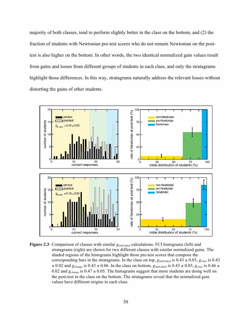
In Figure 2.3, we highlight two classes with virtually identical values of gindividual. The
histograms suggest that more students are doing well on the post-test in the class on the bottom.
Stratagrams reveal that (1) students with non-Newtonian pre-test scores, who compose the
30
majority of both classes, tend to perform slightly better in the class on the bottom, and (2) the
fraction of students with Newtonian pre-test scores who do not remain Newtonian on the post-
test is also higher on the bottom. In other words, the two identical normalized gain values result
from gains and losses from different groups of students in each class, and only the stratagrams
highlight those differences. In this way, stratagrams naturally address the relevant losses without
distorting the gains of other students.
Figure 2.3: Comparison of classes with similar gindividual calculations. FCI histograms (left) and
stratagrams (right) are shown for two different classes with similar normalized gains. The shaded regions of the histograms highlight those pre-test scores that compose the corresponding bars in the stratagrams. In the class on top, gindividual is 0.43 ± 0.03, gclass is 0.43 ± 0.02 and gchange is 0.43 ± 0.06. In the class on bottom, gindividual is 0.43 ± 0.03, gclass is 0.46 ± 0.02 and gchange is 0.47 ± 0.05. The histograms suggest that more students are doing well on the post-test in the class on the bottom. The stratagrams reveal that the normalized gain values have different origins in each class.

31
Figure 2.4: Comparison of classes with differing student populations. FCI histograms (left) and
stratagrams (right) are shown for three different classes with different student populations. The shaded regions of the histograms highlight those pre-test scores that compose the corresponding bars in the stratagrams. In the class on top, gindividual is 0.1 ± 0.1, gclass is 0.1 ± 0.2 and gchange is 0.30 ± 0.05. In the class in the middle, gindividual is 0.479 ± 0.009, gclass is 0.47 ± 0.02 and gchange is 0.48 ± 0.01. In the class on bottom, gindividual is 0.68 ± 0.02, gclass is 0.69 ± 0.02 and gchange is 0.67 ± 0.08. These three classes have very different student populations that are masked by normalized gain values, but the stratagrams highlight the population differences.

32
Finally, in Figure 2.4, we show three classes with very different student populations and
normalized gain values. The histograms show that the student populations of these three classes
are not the same—indeed, the distribution of students in two of the three classes are skewed by
the test ceiling—but the values of gindividual mask all of those differences. The stratagrams,
however, reveal differences in the student population that might affect performance. These
differences are important because students with higher pretest scores tend to exhibit a higher
degree of loss. Additionally, normalized gain values may, in fact, vary with pre-test score
(Coletta & Phillips, 2005). Thus, stratagrams enable users to easily make comparisons between
classes with very different student populations.
2.5 Discussion
The analysis presented here draws a sharp distinction between studies involving many classes
and studies involving only a few classes. The large correlations between gclass and gindividual
support the notion that these definitions are interchangeable when the number of classes under
consideration is large. However, as demonstrated by our pairwise analysis, using different
calculations of g can significantly impact the interpretation of any given comparison between
two classes.
We have already detailed several specific benefits of using stratagrams for pairwise
comparisons among classes. In this section, we discuss some limitations of our analysis and
describe this work in relation to other efforts to study and improve our understanding of student
performance on concept inventories like the FCI.

33
2.5.1 Limitations
Stratagrams have many benefits as a basis of comparison among classes, but they do not convey
all information about a class. The plots suppress the total number of students in the class, and
instead represent them as fractions of the whole, primarily to simplify the plot and suppress
extraneous details. However, this is not to suggest that class size does not matter when two
classes are being compared. We also suppress the number of students who transition from non-
Newtonian to pre-Newtonian levels of performance both to simplify the plot and to emphasize
that the goal of an introductory mechanics course is to acquire a coherent Newtonian force
concept, so improvement in performance that falls short of that goal is of less interest when
comparing classes.
Others have noted that the authors of the FCI provide no concrete evidence for the thresholds
they put forward (Antti Savinainen and Philip Scott, 2002; Dancy, 2000), and that students who
performed well on the FCI do not necessarily exhibit Newtonian thinking in other contexts
(Mahajan, 2005). Additionally, as shown in our analysis, some students exhibit Newtonian
thinking on the pre-test and then fail to exhibit it on the post-test. In other words, the FCI, albeit
often much more insightful than final exams and other course performance metrics, is not a
perfect discriminator of Newtonian thinking. Performance on the FCI cannot necessarily be
generalized to other contexts, and performance on the FCI, like other tests, is subject to variation.
No single test will capture student understanding. Nonetheless, instructors actually use the FCI,
so it is important that we are able to interpret student responses as effectively as possible.
34
2.5.2 Other Alternatives to Normalized Gain
Model Analysis is a detailed graphical and numerical alternative to the normalized gain (Bao &
Redish, 2006). The approach involves consideration of alternate mental models that students may
employ on subsets of the FCI, as well as consideration of the notion that students can hold
multiple mental models and use any one of them, perhaps inconsistently, with some probability
on any given item. Model Analysis involves the calculation of density matrices to determine
probabilities, and it also hinges on qualitative investigations of student reasoning to establish the
mental models in play.
Another alternative means of assessing FCI performance involves item response theory
(IRT), in which students’ total scores establish their ability level and the fraction of students who
respond correctly on each item (as a function of ability level) is used to determine the difficulty,
likelihood of guessing and degree of discrimination achieved by each item (Wang & Bao, 2010).
With separate populations of students, IRT does not readily allow instructors to compare
different courses to one another. However, if populations are pooled together so that ability
levels of students from different classes are on the same scale, then the average ability level of a
class or the shift in average ability level of a class can be used to compare multiple classes.
A similar tool for investigating questions is the analysis of item response curves (IRC)
(Morris et al., 2006). These curves represent a less rigorous alternative to IRT; they permit item-
level analysis of trends in both correct and incorrect responses without use of the assumptions
and statistical methods of IRT. In the case of IRC, students’ performances represent their ability
levels. Although the simplicity of this approach may be appealing, the average student
performance for a given class is no different than simply averaging those students’ scores. Thus,

35
although the insights about various items on the FCI may be informative, IRC does not provide
more insight into comparisons among classes.
Finally, one might also consider comparing the effect size of the change in performance
among different classes (L. Deslauriers, E. Schelew, and C. Wieman, 2011). This approach is
more statistically rigorous than normalized gain as a means of comparing the difference between
two distributions, though problems may still arise when classes are either high-performing or
low-performing, in which cases the skewed distributions may diminish the validity of effect size
as a basis of comparison.
There are strengths to all of these methods. Model Analysis allows for very detailed analysis
of the progression of student reasoning through FCI assessment, but the method is somewhat
complicated and requires qualitative interview analysis to establish anticipated mental models.
IRT and IRC analyses are largely focused on investigating the survey itself, though IRT allows
for calculation of different kinds of gain (ability level rather than performance) that does not
encounter the challenges of loss and ceiling effects that hinder normalized gain. Effect size
captures the same phenomenon, too, but none of these methods convey the same information as
stratagrams. Stratagrams are unique in that they allow for comparisons between classes but do
not mask the differences that may exist. Furthermore, they convey information about student
performance on an absolute scale. Ultimately, we believe that all of these approaches have clear
merit and distinct goals, and therefore complement one another in revealing the most from
student performance on the FCI.

36
2.5.3 Other Conceptual Inventories
All of our analysis and discussion has focused on the FCI. Stratagrams are tailored to the FCI in
order to more strongly motivate the arguments presented here, but one can use a generalized
version of stratagrams to analyze any conceptual inventory in which scores can be binned
according to level of performance. The different groups into which scores are divided (non-
Newtonian, pre-Newtonian and Newtonian, in the case of the FCI) must be consistent across
classes under comparison, but the specific thresholds may not be so important. If the survey is
designed without a specific threshold for success, then one can modify the stratagram as follows:
rather than the height of each bar representing the fraction of students who cross a threshold, the
height can correspond to the average post-test score for the sub-set of students within that
particular pre-test group or bin. Such a plot conveys the same information as the calculation of
non-normalized gain, but with the addition of separating students by initial performance and
highlighting the initial-performance distribution of the class.
2.6 Conclusion
Stratagrams are simple visualizations of student performance that highlight the rate of students
becoming Newtonian thinkers, and therefore provide a clear, informative basis for both assessing
a single class and comparing performance among a small number of classes. Normalized gain is
certainly useful when many different classes are involved; the large correlations among the three
differing means of calculating g support this claim. However, data show that several factors,
particularly losses and differences in pre-test performance, complicate the interpretation of
normalized gain when it is used to compare FCI performance between small numbers of classes.
In such comparisons, fluctuations among different calculations of normalized gain are not

37
negligible and can significantly affect the outcome. Moreover, none of the variations of
normalized gain address the fact that users of normalized gain cannot say which students in the
class are improving, and none of them highlight differences in student population. Thus,
stratagrams fill an instructive, accessible and previously unexplored niche in the array of tools
that are available to instructors for learning the most from student performance on pre-test and
post-test conceptual inventories like the FCI.

38
Chapter Three
Understanding Confusion
Physics instructors typically try to avoid confusing their students. However, educators have
challenged the truism, "confusion is bad," dating as far back as Socrates, who asked students to
question assumptions and wrestle with ideas. So, is confusion good or bad? How should
instructors interpret student expressions of confusion?
During two semesters of introductory physics that involved Just-in-Time Teaching (JiTT)
and research-based reading materials, we evaluate performance on reading assignments while
simultaneously measuring students’ self-assessment of their confusion over the material. We
examine the relationship between confusion and performance, confidence in reasoning, pre-
course self-efficacy and several other measurable characteristics of student engagement. We find

39
that student expressions of confusion are negatively related to initial performance, confidence in
reasoning and self-efficacy, but positively related to final performance when all factors are
considered simultaneously.
3.1 Introduction
When posing the question, “Is anyone confused?” the instructor is implicitly asking students to
engage in the act of monitoring their own understanding, or metacognition (Flavell, 1979).
Students must think about the material, consider with which parts they feel very comfortable and
with which parts they struggle, and then report their findings back to the instructor. Despite how
simple the question seems, a breakdown anywhere along the series of steps that students
undertake in responding may cause the student to reply in a misleading way. This notion may be
familiar to instructors who pose such questions before a quiz, address any confusion (if students
even pose questions), but find that students do not perform very well on the quiz at all.
Of course, students’ minds are not the only places where such “confusion” assessments can
fail. Even if students respond by considering their understanding and posing any questions that
arise, instructors may not interpret such feedback from their students constructively. Students’
questions and expressions of doubt may indicate discomfort with the material, and that more
time and activities should be devoted to addressing these questions. On the other hand, questions
and expressions of doubt may indicate that students are actually engaged and growing familiar
enough with the material that it is conflicting with their prior knowledge and expectations.
Student recognition of this disequilibrium may assist, rather than inhibit, the learning process (J.
Piaget, 1985; J. Piaget, Green, Ford, & Flamer, 1971; Jean Piaget, 1977). If this is the case,
instructional efforts could shift to questions that students have yet to ask themselves. In other

40
words, we cannot yet say whether confusion indicates that things are going poorly or at that
things are going well.
Our primary research question is, “How do students’ expressions of confusion relate to other
measures of learning and engagement?” We acknowledge that expressions of confusion are not
the same as students’ internal confusion, and we also acknowledge that confusion may convey
many things, both good and bad. From a practical point of view, the question posed is fairly
straightforward. However, from a theoretical point of view, as we shall see in the subsequent
section, the variable confusion transects several different theoretical domains. We explore these
domains, present our results, and then analyze our findings in light of both practical and
theoretical concerns.
3.2 Background
The study of metacognition, monitoring one’s own understanding, plays an important role in
addressing our research question. Additionally, the study of confidence and the study of self-
efficacy, belief in one’s ability to perform a skill or do something, shed light on the sometimes-
surprising student responses (or lack of responses) to instructor-posed questions of confusion.
Thus, we introduce these three concepts as an integrated theoretical framework for this study –
metacognition, confidence and self-efficacy – by emphasizing their links to each other and to our
primary research question.
3.2.1 Metacognition
There are two primary aspects of metacognition: (1) knowledge and beliefs about cognitive
phenomena and (2) the regulation and control of cognitive actions (Garofalo & Lester, 1985;

41
Resnick, 1976). The former aspect includes beliefs about oneself and others, knowledge of the
requirements of the task at hand and awareness of strategies and their usefulness for carrying out
certain tasks. The latter aspect is focused on the application of such knowledge and beliefs to the
action of carrying out a cognitive task or problem. Expressing confusion, for example, implies
that one has knowledge of such cognitive phenomena and can regulate (i.e., identify
shortcomings) one’s abilities.
Metacognition is important to the process of learning for the following reason (Everson &
Tobias, 1998):
The learner usually has to master a great deal of new knowledge in a limited amount of time. Moreover, learning in classrooms or other structured training environments is often dynamic, with knowledge and information being updated frequently. Clearly, those who accurately distinguish between what they have already mastered and what is yet to be learned have an advantage in these situations, since they can be more strategic and effective learners. (p. 66)
Everson and Tobias assess metacognition, or knowledge monitoring ability (KMA), by
evaluating the difference between students’ estimates of their knowledge and their performance.
They find that this ability is, in general, positively related to GPA, though in some groups the
relationship was not very strong or statistically significant (Everson & Tobias, 1998). Questions
of validity arise when students are expected to be consistent with one another in how they self-
report about their thinking, as individuals may vary in the weight they assign different criteria or
the manner in which they use the scale (Ward, Gruppen, & Regehr, 2002).
In an effort to promote metacognition in science education, Schraw and colleagues discuss
the concept of self-regulated learning, our ability to understand and control our own learning
environments (Schraw, Crippen, & Hartley, 2006). This concept is rooted in social-cognitive
learning theory, in which learning results from personal, environmental and behavioral factors
(Bandura, 1977). In this model, individuals advance through levels of development that focus on

42
external, social standards (observation, followed by imitation) to levels that depend upon internal
standards (self-control, followed by self-regulation). When an individual is self-regulatory, the
learning process involves three main components: cognition, metacognition and motivation.
Rickey and Stacy connect the discussion of whether students’ questions and statements are
cognitive or metacognitive to the question of whether students’ knowledge is consistent or
fragmented (Rickey & Stacy, 2000). They argue that more metacognitive students are more
likely to recognize inconsistencies and refine naïve ideas. Specifically regarding physics, Koch
emphasizes that a student must understand every word, not just most of them, in a physics
textbook in order to understand the content without misconceptions, because physics text and
content is very different from other texts that students encounter (Koch, 2001). Koch observes
that adding metacognitive tasks to reading-comprehension exercises results in higher post-test
scores when compared to a group of subjects who do not complete the metacognitive tasks, and
therefore argues that metacognition and self-regulation of thinking during reading is an essential
part of reading comprehension. Enhanced reading comprehension helps students monitor their
reading level by themselves and wean themselves away from dependence on teacher evaluation
(Koch, 2001).
More generally, research on involving strong and weak readers, writers and problem solvers
shows skilled, successful individuals also tend to be more successful in metacognitive activities
(Sinkavich, 1995). Kruger and Dunning describe several studies in which they find that
individuals who perform poorly do not know how poorly they are performing (Kruger &
Dunning, 1999). The researchers attribute individuals’ the lack of awareness of the extent of poor
performance to links between content knowledge and the metacognitive skills related to that
knowledge.
43
Several of these studies embed their own explanations of the role of metacognition in
language of “misconceptions” and “naïve ideas.” However, as described in Chapter One, the
suggestion that students’ knowledge is coherent and robust – even if incorrect – is not well-
supported by recent studies (diSessa, 2006). Changes in context and shifts in the manner in
which students frame the activity can alter what they appear to “know” (Redish, 2004).
Therefore, as we consider the role of metacognition and metacognitive activities in student
learning, we must not neglect other theories that we draw upon in our explanations.
3.2.2 Confidence
Confidence refers to one’s belief in one’s own ability to act in a proper or effective way
(Merriam-Webster, Inc, 2003). Researchers have investigated “metamemory” and metacognition
by investigating the relationship between student confidence and performance. Sinkavich reports
a positive correlation between confidence and correctness on an examination, and also notes that
better performing students are more able to accurately predict what they do and do not know
(Sinkavich, 1995). In the experiment, which involves an examination, students are given several
“replacement questions” that can be included for grading instead of questions in which students’
confidence is particularly low; students are required to make this decision and choose the
questions to be replaced themselves. Thus, one can assess whether students have a good sense of
which questions they do not know. In spite of the positive relationship between confidence and
correctness, correct students are not always confident about their correct answers (Sinkavich,
1995). To explain these observations in a theoretical context, Sinkavich employs the expression
“feeling of knowing” (FOK) (Hart, 1965), as a proxy for the first of the two primary aspects of
metacognition: knowledge and beliefs about cognitive phenomena. Interestingly, in comparing

44
good students and poor students, the relationship between confidence and correctness is much
stronger with good students, whereas poor students’ correctness does not vary much with
confidence. In other words, good students appear to be better able to monitor their performance.
In the replacement task, however, both good and poor students exhibited comparable ability to
determine which questions should be dropped from the examination.
Similar studies elaborate on the relationship between confidence and performance.
Engelbrecht and colleagues reports a positive relationship, and also reports that students are more
confident in conceptual math problems than procedural math problems, even though there are no
performance differences on the two types of problems (Engelbrecht, Harding, & Potgieter,
2005). Shaughnessy also reports a positive correlation between confidence and correctness and
notes a larger degree of overconfidence among lower-performing subjects (Shaughnessy, 1979).
Dunning and colleagues suggest that (1) relatively difficult tasks tend to yield overconfidence
more often than relatively easy tasks, and (2) high levels of confidence are usually associated
with high levels of overconfidence (Dunning, Griffin, Milojkovic, & Ross, 1990).
Through consideration of the manner in which data is analyzed, we can better understand
these observations. If item difficulty is determined by calculating percentage of subjects who
respond to that item correctly, but merely choosing an answer implies that confidence is at least
50% (assuming two choices), then the confidence cannot match correctness unless subjects are
irrationally choosing the response they believe is less likely to be correct. In other words,
overconfidence is statistically more likely to increase with difficulty. To further explain other
facets of the overconfidence effect, Gigerenzer and colleagues put forward a theory of
probabilistic mental models (PMM) (Gigerenzer, Hoffrage, & Kleinbölting, 1991). In contrast to
cognitive bias research that claims that people are naturally prone to making mistakes in
45
reasoning and memory, their model assumes that people are good judges of the reliability of their
knowledge. They hypothesize that individuals generalize specific questions to broader
categories, situations or contexts and then inductively infer the correct result with some
probability of correctness. Moreover, they propose that item-by-item overconfidence results from
the fact that one may be fairly knowledgeable about each item in a survey but difficult or tricky
items tend to be surprising, so the average correctness is always likely to be lower than the
average confidence. On the other hand, when asked how many items were answered correctly,
Gigerenzer and colleagues suggest that subjects are likely to underestimate in their response, as
long as the questions are representative of environmental occurrence and not selected to be
particularly tricky. They present empirical data to support this theory (Gigerenzer et al., 1991).
These findings are not necessarily at odds with other studies (Kruger & Dunning, 1999), as the
former do not address variations in estimations from students at different performance levels.
3.2.3 Self-Efficacy
According to social-cognitive learning theory, the learning process involves three main
components: cognition, metacognition and motivation (Bandura, 1977). Schraw and colleagues
identify self-efficacy and epistemological beliefs as the two subcomponents of motivation in this
theoretical framework (Schraw et al., 2006). Simply put, self-efficacy refers “people’s judgments
of their capabilities to organize and execute courses of action required to attain designated types
of performance” (Bandura, 1986, p. 391). Although this may seem exactly the same as
confidence – and, indeed, confidence is sometimes used as a measure of self-efficacy – there are
distinct differences between the two constructs.

46
Albert Bandura introduced the term self-efficacy to provide a means of explaining the effect
of performance-based procedures on psychological change, particularly involving cases of
individuals with acute phobias (Bandura, 1977). He emphasizes the importance of experiences of
mastery and effective performance in ultimately changing cognitive processes, with the goal of
establishing a connection between the cognitive structures in individuals’ minds and their
actions. It is not sufficient that an individual believe that certain actions or behaviors will have
specific outcomes; if the individual does not believe in his/her ability to perform such actions,
then the individual does not associate the outcomes with himself/herself.
According to self-efficacy theory, in the case of a person with an acute phobia, simply seeing
an action performed by another (e.g., handling a snake), or even modeling that action, may not
resolve the phobia in the individual if the exercise does not change the individual’s belief in
his/her ability to perform the same action. In the classroom, self-efficacy theory suggests that
students may see a task performed (and even imitate or model that execution) but not actually
change their beliefs about their ability to perform such tasks in general and therefore ultimately
fail to exhibit learning (Andrew, 1998; Lent, Brown, & Larkin, 1984; Multon, Brown, & Lent,
1991; Pietsch, Walker, & Chapman, 2003).
To be specific about the process, Bandura distinguishes between outcome expectancy – a
person’s belief that a certain behavior will lead to certain outcomes – and efficacy expectation – a
person’s belief that he/she can successfully execute the behavior required to produce the
outcomes (Bandura, 1977). If a situation appears to an individual to exceed his/her own ability to
cope with it, the individual tends to avoid that situation or does not persist very long in the
efforts. On the other hand, when people believe they can do something, they tend to be more
persistent at achieving the desired goal or behavior; they locate and enact resources to aid them.

47
Bandura refers to the ability to exercise this control over thought and action as human agency
(Bandura, 1989).
Efficacy expectations have magnitude, generality and strength; these characteristics influence
performance and are, in turn, altered by the cumulative effects of one’s efforts (Bandura, 1977).
Performance accomplishments, one of four primary means of probing and augmenting an
individual’s self-efficacy, bear the most relevance to the activities in a physics classroom and
instructional laboratory; students cannot merely observe certain practices, but must engage in the
activities themselves. Similarly, the other formal means of assessing self-efficacy – vicarious
experience, verbal persuasion and emotional arousal – link to analogous activities in physics
learning environments. Prolonged encounters are more successful than distributed encounters in
effecting change.
Self-efficacy is a broad-reaching theoretical subject that encompasses many elements of
learning and development. Research efforts in physics education indicate that “physics self-
efficacy” plays an important role in both learning and interest in the discipline (Fencl & Scheel,
2004; Sawtelle, 2011). More broadly, Multon and colleagues perform a meta-analysis of data
collected from many studies and find a positive relationship between self-efficacy and academic
performance in the sciences (Multon et al., 1991). This relationship is even stronger between
performance and post-course self-efficacy in studies that distinguished between pre- and post-
course surveys of self-efficacy. In another study, Andrew measures self-efficacy through
evaluations of confidence in various criteria contained within the Self-Efficacy for Science
(SEFS) survey and finds that self-efficacy for sciences is positively related to academic
performance (Andrew, 1998). This study does not account for changes in self-efficacy.
Interestingly, no relationship between expressions of self-efficacy and science background is

48
observed. Lent and colleagues find that self-efficacy compares favorably to other models for
academic success and career decision-making (Lent, Brown, & Larkin, 1987). Additionally, the
perceived importance of self-efficacy beliefs may be stronger for women in male-oriented
domains than for individuals operating in traditional settings (Zeldin & Pajares, 2000), and
differences in self-efficacy are associated with differences in gender performance and
representation (Kost et al., 2009; Sawtelle, 2011).
Researchers distinguish among more general beliefs about competence (self-concept),
attitudes regarding one’s beliefs (self-esteem) and self-efficacy (Linnenbrink & Pintrich, 2003;
Pietsch et al., 2003). Self-efficacy associates behavioral, cognitive and motivational engagement
with learning. Linnenbrink and Pintrich suggest that, ideally, one’s self-efficacy is a bit beyond
one’s ability so that, in attempting to complete tasks, one’s skills are likely to increase; this
suggestion is connected to the notion of “zone of proximal development” (Vygotskiǐ & Cole,
1978), discussed in Chapter One. Overall, the study suggests that self-efficacy is positively
related to adaptive motivational beliefs and positive affective reactions, and negatively related to
negative emotions.
3.2.4 Theoretical to Practical
Several researchers highlight practical implications of the largely theoretical discussion
presented here. To improve student learning outcomes, instructors should engage in inquiry-
based activities, build collaboration among students, provide multiple strategies for
accomplishing goals, emphasize the role of mental models in conceptual change, and build from
students’ and instructors’ epistemological beliefs (Schraw et al., 2006). All of these suggestions
are motivated by the links between self-efficacy, confidence, metacognition and student learning

49
outcomes. If one considers problem solving as grappling with unfamiliar tasks and methods that
are not well-understood (Schoenfeld, 1992), as opposed to the completion of tasks using
prescribed methods, metacognition plays a much more important role (Rickey & Stacy, 2000).
These studies highlight the importance of self-efficacy in the classroom, but they do not
necessarily shed light on the differences between self-efficacy, confidence and, the construct that
is ultimately of the most interest to us, confusion. We have no formal reason to believe that
measures of confidence and self-efficacy are distinct; perhaps a student’s expression of
confidence is simply indistinguishable from a student’s expression of self-efficacy in that same
ability. Some argue that self-efficacy is very specific to a task in a given situation while the term
self-concept, described above, actually applies to more general beliefs about competence
(Linnenbrink & Pintrich, 2003). In contrast, others refer to self-efficacy as a more general sense
of one’s ability (e.g., in science), and even Bandura mentions that performance accomplishments
in multiple contexts can effectively improve self-efficacy across contexts (Bandura, 1977). Thus,
the lines between self-concept and self-efficacy, or confidence in one’s ability and confidence in
one’s actions in a specific circumstance, are not entirely clear from the vocabulary employed in
the theoretical frameworks. Nomenclature aside, we can say that the distinction in meaning
between general and specific conceptions of ability and performance exists.
The concept of confusion, from a theoretical viewpoint, is even more muddled. Expressions
of confusion blend cognitive and metacognitive aspects of students’ knowledge, as well as
elements of self-efficacy and confidence at both specific and general scales. Consequently, we
cannot say, a priori, how expressions of confusion interact with such theoretical components;
rather, we explore a series of studies in which data relating confusion, confidence and self-
efficacy are collected simultaneously. Ultimately, we have some basis for discussing confusion
50
in the context of the theories presented here, as well as a means of answering the question of
practical importance to instructors: How do students’ expressions of confusion relate to other
measures of learning and engagement?
3.2.5 Motivation for Analysis
We propose to investigate student expressions of confusion in a sequence of studies that are
closely motivated by an initial study involving similar research questions (C. Crouch, 2000). The
data were collected during courses using two specific instructional strategies, Just-in-Time
Teaching and Peer Instruction
Just-in-Time Teaching
Just-in-Time Teaching (JiTT) is a teaching and learning strategy composed primarily of Internet-
based, pre-class activities and corresponding in-class activities (Novak, Gavrin, & Wolfgang,
1999). Students engage with the material – e.g., complete a reading assignment, watch an
Internet-based video, interact with a simulation – and then complete a “WarmUp” activity the
evening before class. The students’ submissions provide feedback to the instructor before class,
so the instructor has the opportunity to use the class time to focus on student difficulties. These
pre-class activities may consist a brief essay question, an estimation question and a multiple-
choice question – the combination prescribed by Novak and colleagues – or some other
combination of questions.
By shifting the transmission of information from inside the classroom to outside, instructors
are no longer required to “cover” all of the material in class. Rather, they can engage students in
a variety of activities and focus upon only the particularly difficult facets of the material. JiTT

51
developers suggest a combination of in-class activities that includes discussion of student
responses to pre-class exercises, interactive activities and demonstrations.
Peer Instruction
Peer Instruction (PI) is a research-based, interactive teaching strategy that facilitates student
interaction and, specifically, metacognition, in the classroom (Mazur, 1997). Instead of lecturing,
the instructor presents conceptual questions to the students. According to Mazur, “this process a)
forces students to think through the arguments being developed and b) provides them (as well as
the teacher) with a way to assess their understanding of the concept” (Mazur, 1997, p. 10). Each
conceptual question is preceded by a brief presentation of the material and follows this general
format:
(1) the instructor poses the question,
(2) students are given approximately one to three minutes to think about it,
(3) students respond individually,
(4) students try to defend and convince neighboring students of their responses,
(5) students respond individually once again,
(6) and the instructor explains the correct response.
Students may respond using clickers, flashcards or fingers, all of which are equally effective (N.
Lasry, 2008). This strategy provides a stream of feedback on how the students are responding to
the material, and it allows students to communicate ideas and consider multiple perspectives.
Researchers consistently associate PI with improved learning outcomes (C. H. Crouch & Mazur,
2001; Smith et al., 2009).
52
Like the in-class activities associated with JiTT, PI requires that students encounter the
material before coming to class. Accordingly, the pre-class reading assignments associated with
JiTT provide the same feedback to instructors using PI as they provide to instructors using JiTT
alone; in both cases, student responses shape the subsequent in-class activities. In incorporating
the pre-class components of JiTT to PI, Mazur makes one important modification. Instead of the
combination of three questions proposed by Novak and colleagues, he suggests that instructors
ask two content-related questions and one “confusion” question. The confusion question requires
students to reflect on their understanding of the material, and therefore captures a fundamentally
different, unique facet of student engagement.
In subsequent sections, we will detail this feedback question, how it may be posed to
students, and how instructors may best interpret student responses.
Crouch and Mazur (2000)
In their original analysis (C. Crouch, 2000), Crouch and Mazur posed the question, “Does a lack
of confusion indicate understanding?” To investigate this question, they analyzed a single
reading exercise, containing three questions, that was submitted by 151 students. They found that
students who expressed confusion about topics related to the questions appeared to respond
correctly to the content-related questions more than students who did not express such confusion.
However, this original analysis was not intended to be a rigorous evaluation, and therefore
required further analysis before moving on to a full study.
53
3.3 Methods – Pilot Analysis
In order to investigate the results from previous work and better assess our ability to answer the
primary research question, we first reexamine the data collected and analyzed by Crouch and
Mazur. In this pilot analysis, we addressed the following research question: What is the
relationship between students’ performance on the content-related questions and their
expressions of confusion?
In the subsequent full study, we apply the insights from the pilot analysis toward a much
larger question involving many more reading exercises and several additional measures of
student learning and engagement.
3.3.1 Course Information
We analyzed data collected from an introductory physics course at Harvard University during the
fall of 1998. This was the first-semester course in a one-year sequence for non-physics
concentrators. The instructor employed PI and the pre-class components of JiTT. Students
received credit for participation in, but not correctness of, their responses to both pre-class and
in-class questions.
Importantly, in this course, pre-class reading assignments included only free-response
questions. The two content-related questions were intended to be thought-provoking and
counterintuitive, so students would have to critically engage with the material before class.
Questions required students to explain their reasoning. In each assignment, the confusion
question was posed after the two content-related questions.
Students submitted responses online using the Interactive Learning Toolkit (ILT), a course
management platform developed for use with PI and JiTT.
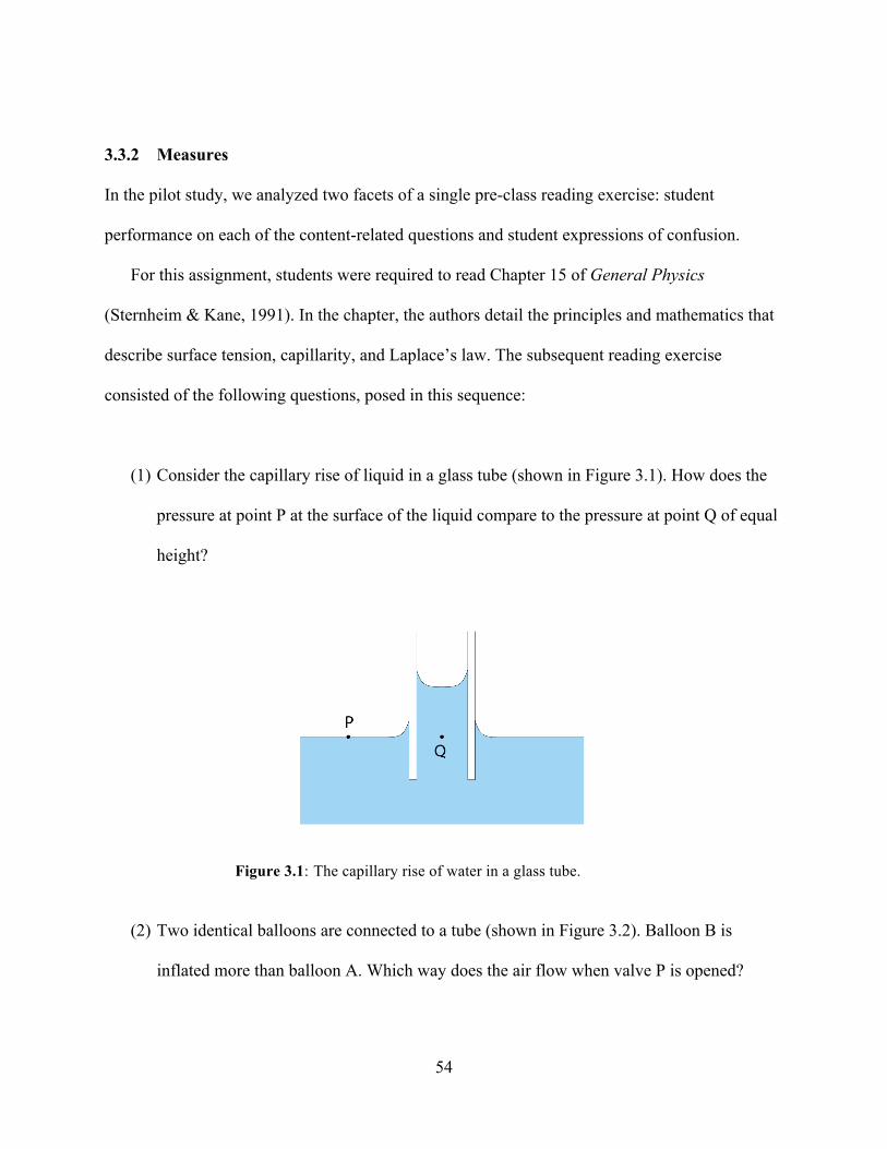
54
3.3.2 Measures
In the pilot study, we analyzed two facets of a single pre-class reading exercise: student
performance on each of the content-related questions and student expressions of confusion.
For this assignment, students were required to read Chapter 15 of General Physics
(Sternheim & Kane, 1991). In the chapter, the authors detail the principles and mathematics that
describe surface tension, capillarity, and Laplace’s law. The subsequent reading exercise
consisted of the following questions, posed in this sequence:
(1) Consider the capillary rise of liquid in a glass tube (shown in Figure 3.1). How does the
pressure at point P at the surface of the liquid compare to the pressure at point Q of equal
height?
Figure 3.1: The capillary rise of water in a glass tube.
(2) Two identical balloons are connected to a tube (shown in Figure 3.2). Balloon B is
inflated more than balloon A. Which way does the air flow when valve P is opened?

55
Figure 3.2: System of two balloons connected by a valve.
(3) Please tell us briefly what points of the reading you found most difficult or confusing. If
you did not find any part of it difficult or confusing, please tell us what parts you found
most interesting.
Students responded to these questions in free-response, short-essay form. Although this format
provides students flexibility in their responses, it allows them to submit correct answers with
incorrect justifications, “incorrect” answers with well-reasoned justifications, and a plethora of
other ambiguous responses. We could have labeled responses “completely correct” or “not
completely correct,” but then correct responses without justification, of which there are many,
could alter the apparent relationship between performance and expression of confusion.
Therefore, instead of subjectively making judgments and labeling responses as “correct” or
“incorrect,” we labeled responses descriptively, according to the outcome stated by the student
(e.g., in question (2), labels included “flows to the left,” “flows to the right,” and “does not
flow”).
We employed a similar descriptive approach in labeling student expressions of confusion. As
detailed in Table 3.1, we coded responses as relating to the textbook (explanation provided,

56
figures, equations, examples, symbols, problems and terminology), concepts (laminar flow,
cohesive forces, surface tension, contact angle, capillarity, Laplace’s law, pressure), the reading
exercise itself (question one and question two), general goals and “real world” applications,
which means the response relates to connecting the formal content to actual practices. Different
concepts are associated with different sections of the text: Sections 15.1 and 15.2 relate to the
concepts of contact angle, surface tension and capillarity; Section 15.3 relates to the concept of
Laplace’s law; and later sections relate to other, more applied concepts. A single response may
require multiple labels.
Table 3.1: Codes used to label student responses to confusion question.
textual section conceptual section other section
explanation any laminar flow 14 question 1 15.1 and 15.2
figures any cohesive forces 15.1 question 2 15.3
equations any surface tension 15.1 objectives any
examples any contact angle 15.2 applications 15.2 or 15.4
symbols any capillarity 15.2 not confused none
problems any Laplace’s law 15.3
terminology any pressure 15
By coding expressions of confusion this way, we are able to sort the responses according to
several different criteria: textual vs. conceptual, confusion vs. no confusion, and question-related
confusion vs. non-question-related confusion. There are no statistically significant differences in
the proportion of students who respond with the correct answer between groups that express text-
related confusion and concept-related confusion. Thus, we collapse these codes together and

57
focus on the content areas to which the expressions of confusion relate. Because students were
asked to identify only the points they were most confused about, we cannot assume that they
were exhaustive in their responses.
To summarize, students were sorted based only upon these two facets of their responses: the
answer provided to each of the content questions and the explicit sources of confusion identified.
3.3.3 Sample Description
The sample consists of 151 students. As we have access to only the responses of these students to
this pre-class reading exercise, we cannot comment on the relationships among additional factors
(e.g., pre-course knowledge, final grades). Overall, 43 students (28%) responded with the correct
answer to the first content-related question, 37 students (25%) responded with the correct answer
to the second content-related question and 16 students (11%) responded with the correct answers
to both content-related questions. 62 students (41%) expressed confusion related to the first
content-related question, 47 students (31%) expressed confusion related to the second content-
related question, and 39 students (26%) expressed no confusion.
3.3.4 Analytic Methods
To investigate the differences in performance between groups of students who express confusion
about different parts of the reading, we performed chi-squared tests to determine whether there is
an association between the confusion and correctness classifications. This test permits
comparisons between multiple groups. If only two groups are under comparison (i.e., a 2 × 2
table), the z test for comparing proportions between two groups can also be used, though both
tests yield precisely the same result (Moore, McCabe, Duckworth, & Alwan, 2008).

58
Two researchers independently coded students’ free responses to reading exercise questions
and subsequently discussed coding. All discrepancies were resolved during discussion, and the
coding criteria were refined to eliminate future discrepancies. Once the criteria for each code
were sufficiently well established through discussion, remaining reports were coded
independently.
3.4 Results – Pilot Analysis
We compare the proportion of students who responded to each question correctly (i.e., identified
the outcome that we consider “correct”) between groups that express confusion about different
aspects of the reading assignment. Specifically, we made comparisons among students who
express no confusion, students who express confusion unrelated to the question under
consideration, and students who express confusion related to the question under consideration.
Table 3.2: Proportion of students who respond correctly, by expressions of confusion.
Question no confusion non-Q-related confusion
Q-related confusion
chi-square
p value
1 36% (N = 39) 30% (N = 50) 23% (N = 62) 0.338
2 13% (N = 39) 23% (N = 65) 36% (N = 47) 0.041
As shown in Table 3.2, we find no statistically significant relationships between expressions
of confusion and correctness on the first (capillarity) content-related question. Although there are
apparent numerical differences, they are not statistically significant. On the contrary, we do find
a statistically significant relationship between expressions of confusion and correctness on the

59
second content-related question. In this case, the proportion of students who respond with the
correct answer is higher among students who express confusion than among those who express
no confusion, and highest among those who express confusion related to the question.
3.5 Motivation for Full Study
One might argue that only some students who are performing well express confusion because
they are critically engaging with the material; other students may have such a strong grasp of the
material that they perform well without any confusion. Similarly, some poorly performing
students may not know how little they know, while others are so confused that they perform
poorly and can only ask questions. The existence of these different groups within the population
could explain the results presented here.
The data analyzed here were previously studied and presented to motivate the notion that
expressions of confusion may actually be associated with positive course outcomes (C. Crouch,
2000). However, the results presented here differ from those previously presented; we find that
only one of the two questions exhibits a positive relationship between expressions of confusion
and performance, whereas the previous findings suggest that both questions exhibit this
relationship. The source of this discrepancy, detailed below, is in the criteria by which students’
responses are sorted. We also describe several limitations to the implications of this analysis, and
ultimately motivate subsequent full study.
3.5.1 Discrepancies between Analyses
In the analysis by Crouch and Mazur, students’ expressions of confusion were sorted as “related”
or “unrelated” to each of the content-related questions. Expressions of confusion about

60
capillarity and pressure are labeled as “related” to the first question, but expressions of confusion
about closely-related topics like contact angles and cohesive forces were not. Moreover, general
statements (e.g., everything was confusing) and specific statements (e.g., the question itself was
confusing) were also labeled as “unrelated.” Coding according to such criteria necessitates
making several assumptions about students’ intent when they make specific statements. In the
analysis presented here, we carefully avoid these assumptions using the coding scheme presented
in Section 3.3.2. Using these descriptive labels of statements made by students – in contrast to
evaluative (or assumptive) labels – allows us to code each response objectively. Only at the end,
after coding is complete, do we determine which descriptive codes – not individual responses –
should be considered “related” or “unrelated” to each question. Also, as described in Section
3.3.4, multiple researchers worked together to establish the objective validity of the coding
criteria presented here. Therefore, the two analyses of the same data differ.
One might argue that this post-coding determination of whether particular expressions of
confusion are related to each of the content-related questions could affect the observed
relationships. To test this, we also consider different comparisons in our analysis: (1) students
who express no confusion and students who express confusion, and (2) students who do not
express confusion related to the question under consideration and students who do express
confusion related to the question under consideration. The results of these alternate sorting
criteria agree with the results presented above; therefore, the post-coding determination does not
significantly alter the observed relationships.

61
3.5.2 Limitations of Pilot Analysis
Although the hypothesis introduced above is a viable explanation for these results, it is certainly
not the only one. Limitations include: (1) the inability to control for other, potentially significant
background variables, (2) the specific way in which questions were posed, and (3) the fact that
this reading exercise is only one measurement.
A more general metric like the final exam or final grade may better represent student learning
or performance, as the reading exercises were not actually evaluated for correctness. The
willingness to express confusion may relate more directly to confidence in one’s abilities than to
performance in the course. These additional variables, among others, could significantly inform
– or even alter – the observed relationships.
Even the information we have limits our ability to draw conclusions from the results. As
noted above, students were only asked what they found most confusing. The group of students
who express confusion that is unrelated to the content-related question under consideration may
be actually composed of students who are less confused and students who are not confused about
the question. If this is the case, the proportion of the students who respond with the correct
answer from each of these groups may significantly alter the results.
As this assignment is essentially one data point – there are 151 students, but only one reading
exercise – there are numerous alternative hypotheses that account for the observed results. The
first question, although challenging, does not necessarily require students to understand
capillarity to respond correctly; it is sufficient to recognize that the pressure must be equal at
equal heights in a static system. Therefore, expressions of confusion may not correlate with
confusion about capillarity for this reason, which has nothing to do with students’ metacognition.
The second question, for different reasons, does not require students to understand Laplace’s

62
law; the correct response is simply stated in the text. Students may have completed the reading
assignment and, appearing to “perform” better than their peers who did not complete the reading
assignment, express confusion about the subject. In other words, one question is only
superficially related to the material the other question can be answered directly from the reading
without any understanding. This may explain why we observe a different pattern of results in the
two questions. Moreover, there is no evidence to suggest that students who express no confusion
simply did not complete the reading assignment.
We attempt to address all of these shortcomings in the full study, which we describe in the
subsequent section. However, some of these challenges stem from the fact that we simply cannot
know what students do not say. We can study and interpret expressions of confusion, but we
must always acknowledge that students’ expressions of confusion may not precisely correspond
to confusions that they have in mind. Only the former, however, is a candidate for assessment of
student learning.
3.6 Methods – Full Study
There are several important differences between the pilot analysis and the full study. In the pilot
analysis, all of the student responses were entirely free-response. This format is highly conducive
to rich student responses, but, barring automated text analysis, we cannot analyze large amounts
of such data without a tremendous amount of work. Therefore, in the full study, we modified the
format of the questions so that student responses can be analyzed efficiently without sacrificing
the detailed information afforded to instructors by the free-response format. This choice allowed
us to analyze 43 reading exercises collected over two semesters of instruction.

63
We designed the questions so that students must critically consider the material (or guess
correctly) in order to respond correctly; none of the answers are simply buried in the reading
assignment. Moreover, each question requires students to consider content specific to the reading
assignment, to avoid the situation in which students can reason correctly using other content
knowledge.
3.6.1 Course Information
We analyzed data collected from both semesters of a two-semester sequence of introductory
physics courses at Harvard University during the fall of 2010 and the spring of 2011. This
sequence of courses was designed for non-physics concentrators. A different instructor taught
each semester. Both instructors implemented the pre-class components of JiTT and emphasized
the importance of completing the reading assignments to the students. The instructor of the first-
semester course occasionally posed in-class conceptual questions to students for discussion, but
more often presented material through lectures and demonstrations. The instructor of the second-
semester course employed PI; demonstrations were used in conjunction with in-class conceptual
questions and discussion, and use of lecture was limited. In both semesters, students received
credit for participation by responding to both pre-class exercises and in-class questions.
Just as in the pilot study, reading assignments consisted of two content-related questions and
a confusion question. The two content-related questions were intended to be thought-provoking
and counterintuitive, so students would have to critically engage with the material before class.
Questions required students to explain their reasoning. In each assignment, the confusion
question was posed before the two content-related questions, followed by a final opportunity to

64
revise the response to the initial confusion question. Students submitted responses online using
the ILT.
3.6.2 Measures
In the full study, we analyzed the same two facets of the pre-class reading assignment that we
studied in the pilot analysis – student performance on each of the content-related questions and
student expressions of confusion – in addition to many other dimensions of student
characteristics and course performance. Specifically, we analyzed pre- and post-course
performance on the Force Concept Inventory (FCI) or Conceptual Survey of Electricity and
Magnetism (CSEM), performance on course-related activities (problem sets, laboratory
activities, exams and cumulative grades), and measures of student confidence collected as part of
the reading assignments. Additionally, in the spring semester, we analyzed pre- and post-course
performance on a survey of self-efficacy in physics.4
Conceptual Surveys
In the fall semester, the FCI was administered to assess students’ conceptual understanding of
Newtonian mechanics (Hestenes et al., 1992). In the spring semester, the CSEM was
administered to assess students’ conceptual understanding of electrostatics and magnetostatics
(Maloney et al., 2001). Both surveys consist of a series of multiple-choice questions that are
4 We also administered the Data Handling Diagnostic (DHD) in conjunction with the comparative laboratory study that is discussed in Chapter Four. As we discuss later, the DHD appears to assess a dimension of student engagement that is not probed by the other metrics highlighted here; student expressions of confusion are strongly negatively correlated with pre-test performance on the DHD, even when other variables described here are included in the model. However, inclusion of the DHD does not qualitatively change the relationships between confusion and these other variables, and therefore only complicates the present investigation. Therefore, we note the significance of the DHD but exclude it from the present analysis, in favor of discussing it further in Chapter Four.
65
designed to elicit students’ intuitive ways of thinking – which may or may not be correct –
through the use of “everyday” language instead of terminology typical of the physics classroom
and response choices that appeal to empirically-identified incorrect ways of reasoning. We
present a more thorough discussion of such surveys – and the FCI, in particular – in Chapter
Two. The survey is administered as a pre-course assessment during the first week of the semester
and as a post-course assessment sometime after the final class meeting and before the final exam.
Both surveys are administered through the Internet-based ILT; students have 45 minutes to
complete each survey. They received credit for participation, but not for correctness.5
Course-Related Performance
If we were to include all of the criteria representing various aspects of students’ performance on
course-related activities in our analysis, many of the factors would be redundant. Therefore, we
employ the statistical technique of factor analysis to determine if the correlations among
different variables actually describe one or more uncorrelated aspects of performance (Costello
& Osborne, 2005).
For both the fall and spring semesters, we find that reading exercises (evaluated for
participation only), laboratory activities, mid-term exams, final exams and final grades all
describe virtually one factor; the difference between the first and second eigenvalues is much
larger than the differences between subsequent eigenvalues. The final exam and final grade are
weighted most heavily in determining that factor. Therefore, for simplicity and clarity, we
5 Based on our analysis in Chapter Two, perhaps we could treat these conceptual surveys as categorical variables. Indeed, this approach has been done by others (Watkins, 2010). However, in our analysis, we are primarily interested in examining students’ pre-course performance, in which there are no ceiling effects. Therefore, we are not inclined to complicate the interpretation of our analysis, while simultaneously suppressing potentially relevant information, if we do not need to do so.

66
choose to employ final grade as the primary summative measure of students’ performance in the
course.
Reading Exercises
In order to collect as much information as possible with each reading exercise, we significantly
modified the format from that which was used in the pilot study. The confusion question was
moved to the beginning of the exercise and consisted of three parts. The question was posed as
follows:
(1) In the material that you just completed, did you find anything difficult or confusing?
[students select “yes” or “no”]
(2) Which parts were [if “yes” was selected, the word “confusing” appears here; if “no” was
selected, the word “interesting” appears here]?
[for each section from the reading assignment, students select “not at all,” “somewhat” or
“very”]
(3) Please elaborate. Do you have any questions?
Asking the question this way serves multiple purposes. By asking students if they are confused
and gauging their confusion on the various topics in the reading assignment, the question is more
thorough than simply asking which points students found most confusing. Although we cannot
claim that all students interpret this question the same way, we no longer have to wonder
whether students neglect to express particular confusions because they are merely less confused
or, in fact, not confused about those topics. Of course, the free-response information is most

67
valuable to the instructor before each class, so the third part of the confusion question ensures
that students can be specific as well as thorough, without too much effort.
We established a quantitative value for confusion based on students’ responses to their
degree of confusion about topics within a reading assignment. “Not at all,” “somewhat,” and
“very” are associated with the numerical values 0, 1, and 2, respectively, and these values are
averaged across all topics listed within a single reading assignment. We call this average value
the confusion index. If a student expresses no confusion, the confusion index is zero. If a student
(1) expresses confusion and (2) is “somewhat” confused about one of two topics and “not at all”
confused about the other, that student’s confusion index is 0.5. If a student expresses confusion
and is very confused on all topics, the confusion index is 2. In this way, we can quantify the
degree of confusion of different students.6
The content-related questions that follow the confusion question were modified as well. At
least two – and sometimes as many as three or four – researchers and instructors reviewed and
discussed each question to ensure that they depend upon the content in the reading but cannot be
answered by simply locating a key passage in the text. Whenever possible, questions were
designed so that the entire space of possible answers could be spanned by the response choices
(e.g., A greater than B, B greater than A, A and B are equal). This way, each question could be
posed as a multiple-choice question with a free-response field for students to explain their
reasoning, and the answer choices do not necessarily influence students’ reasoning. Thus,
6 One might wonder why we should calculate students’ confusion indices when we have already asked them if they are confused. The ability to characterize the degree of confusion is certainly valuable, though the yes/no response that precedes it is even easier to interpret. However, degree of confusion is better-suited for statistical analysis; students tend to express some confusion relatively frequently, so the yes/no variable is much more skewed toward the upper limit than the confusion index, which is more normally distributed. Therefore, in our analysis, we will characterize student confusion using the confusion index variable; any subsequent references to “confusion” should be interpreted as “average degree of confusion.”
68
ideally, we collect readily compiled information and do not direct students to one particular
manner of addressing the problem. We approached question development this way because we
recognize that instructors often cannot guess what alternate answer choices are going to attract
students, but we did not have time to conduct student interviews and establish empirically-based
alternate responses for each question.
In posing the content-related questions this way, we also probed one more facet of student
understanding: confidence. After explaining their reasoning, students were asked to rate their
confidence in the reasoning that they provided on a scale of low, medium and high. These levels
were associated with respective numerical values for quantitative analysis.
All of these numbers – confusion indices, correctness, and confidence – convey important
information about a single reading assignment. However, if variations from one exercise to the
next result in negligible correlations between them, then we have no basis for computing and
discussing averages. We conduct factor analysis once again on these variables and find that all of
the individual confusion indices, correctness values and confidence ratings are strongly described
by one factor, respectively. Again, the difference between the first and second eigenvalues is
much larger than the differences between subsequent eigenvalues. Therefore, we can safely
describe students’ averages as representative of the underlying common factor in their individual
reading exercise responses.
All of the content-related questions from the reading exercises from both semesters, along
with the associated topics of potential confusion, are included in Appendix A.
69
Self-Efficacy Survey
This survey, administered as a pre-test during the first week of classes on paper and as a post-test
between the last class and the final exam via the Internet, was designed to measure both
“physics” self-efficacy and “Peer Instruction” self-efficacy. It was based on a similar survey
designed to assess physics self-efficacy (Fencl & Scheel, 2004). Seven of the questions related
explicitly to students’ belief in their ability to perform physics-related activities, and eight of the
questions related explicitly to students’ belief in their ability to engage in Peer Instruction
activities. Students responded to questions on a Likert scale (five-point scale from strongly
disagree to strongly agree).
The survey was implemented both to assess students’ physics self-efficacy and to investigate
whether students’ exhibit Peer Instruction self-efficacy. Only the former is related to our primary
research questions – and the latter is the subject of ongoing research – so we only consider the
first series of questions, related to physics self-efficacy, in our analysis. This survey was only
administered in the spring semester, so we do not consider self-efficacy of students during the
fall semester.
To summarize, in this full study, we analyze student expressions of confusion, performance
on reading exercises, confidence in their performance on reading exercises, pre- and post-course
self-efficacy, pre- and post-course conceptual understandings and performance on graded course
activities.
3.6.3 Sample Description
Students completed 22 reading exercises during the fall semester and 21 reading exercises during
the spring semester. Data from 139 students were analyzed: 109 from the fall semester and

70
approximately 90 from the spring semester, of which 60 were enrolled in both semesters. Not all
students completed all surveys and not all students completed the course, which explains why we
have more reading exercise data than reported final grades.
Table 3.3: Descriptive statistics of characteristics of student learning and engagement, Fall 2010.
variable N mean median s.d. range
confusion index 109 0.45 0.43 0.26 0.00 – 1.10
correctness 109 0.77 0.76 0.19 0.32 – 1.37
confidence 109 2.20 2.21 0.32 1.24 – 3.00
FCI, pre 97 17.90 18 6.75 4 – 30
FCI, post 78 22.19 23 6.39 3 – 30
final grade 106 100.57 102.70 17.36 42.11 – 125.99
Table 3.4: Descriptive statistics of characteristics of student learning and engagement, Spring 2011.
variable N mean median s.d. range
confusion index 90 0.57 0.60 0.31 0.06 – 1.68
correctness 90 0.85 0.85 0.26 0.30 – 1.62
confidence 90 2.06 2.03 0.39 1.00 – 2.93
CSEM, pre 72 12.76 12 5.73 2 – 27
CSEM, post 55 21.95 23 6.76 6 – 32
final grade 89 85.36 86.44 8.76 57.63 – 99.29
self-efficacy, pre 88 3.51 3.57 0.73 1.14 – 5.00
self-efficacy, post 81 3.45 3.43 0.72 1.00 – 5.00

71
Table 3.3 and Table 3.4 display descriptive statistics for the measures described in Section
3.6.2. The confusion index, correctness and confidence variables represent the mean for each
student across all reading assignments. Accordingly, the average values displayed below are
“averages of the averages” of these variables.
3.6.4 Analytic Methods
We investigated the relationships among these factors using multiple regression analysis. Also,
as described above, we employed factor analysis techniques to establish which course
performance measures should be retained, as well as to justify our use of average confusion
indices, confidence ratings and correctness values in our multiple regression models.
For much of the analyses presented here, we calculated the standard score, or z-score, for
each of the variables before carrying out multiple regression analysis. The standard score is a
representation of the variable after it has been rescaled according to the following equation:
€
z =x − µσ
, (3.1)
where x is the original variable, µ is the mean of the distribution, σ is the standard deviation of
the distribution and z is the standard score. We rescale these values for several reasons.
Particularly in the cases of such variables as confusion index, confidence and self-efficacy, the
native scales are not readily interpretable, so we can more easily describe observations using
standard scores. Analyzing standard scores allows us to compare the relative strength of
relationships among variables with different units. However, standard scores can mask whether
or not a relationship is meaningful on an absolute scale. Thus, we consider both absolute and
standard scores in our analysis. Multiple regression techniques are equivalent, regardless of
scale; the calculated coefficients change, but the statistical significance does not.

72
3.7 Results – Full Study
Whereas the pilot analysis discussed above focused only on the relationship between confusion
and correctness, the present analysis involves multiple variables and many different
relationships. Thus, we first investigate the pairwise correlations among variables discussed
above, for both the fall and spring semesters.7
Table 3.5: Pairwise correlations of characteristics of student learning and engagement, Fall 2010.
confusion index correctness confidence FCI, pre FCI, post final grade
confusion index 1.00
correctness -0.25** 1.00
confidence -0.41*** 0.34*** 1.00
FCI, pre -0.32** 0.58*** 0.27** 1.00
FCI, post -0.24* 0.57*** 0.21 0.71*** 1.00
final grade -0.04 0.45*** 0.24* 0.56*** 0.55*** 1.00 (*p < 0.05, **p < 0.01, ***p < 0.001)
As shown in Table 3.5, during the fall semester, confusion appears to be negatively related to
each of the other variables. The strengths of these relationships vary; confusion appears to be
strongly negatively related to confidence and not at all related to final grade. However, we also 7 We consider pairwise correlations because, as shown in Table 3.3 and Table 3.4, participation rates vary across different measures of student learning and engagement. Instead of diminishing our statistical power by limiting analysis to only those students who completed everything, we compare students who completed everything to those who did not complete everything to confirm that the fluctuations in participation do not bias our analysis. Comparisons of the means indicate that the two groups are not significantly different from one another. Therefore, we are confident that our analysis is not biased from fluctuations in participation.

73
see that the variables are strongly related to one another, suggesting that multiple regression
analysis of confusion and these other variables may reveal very different relationships.
We see that relationships during the spring semester, shown in Table 3.6, are very similar to
those observed in the fall semester. Self-efficacy is strongly negatively related to expressions of
confusion, though it is also strongly related to virtually all of the other characteristics under
consideration here.
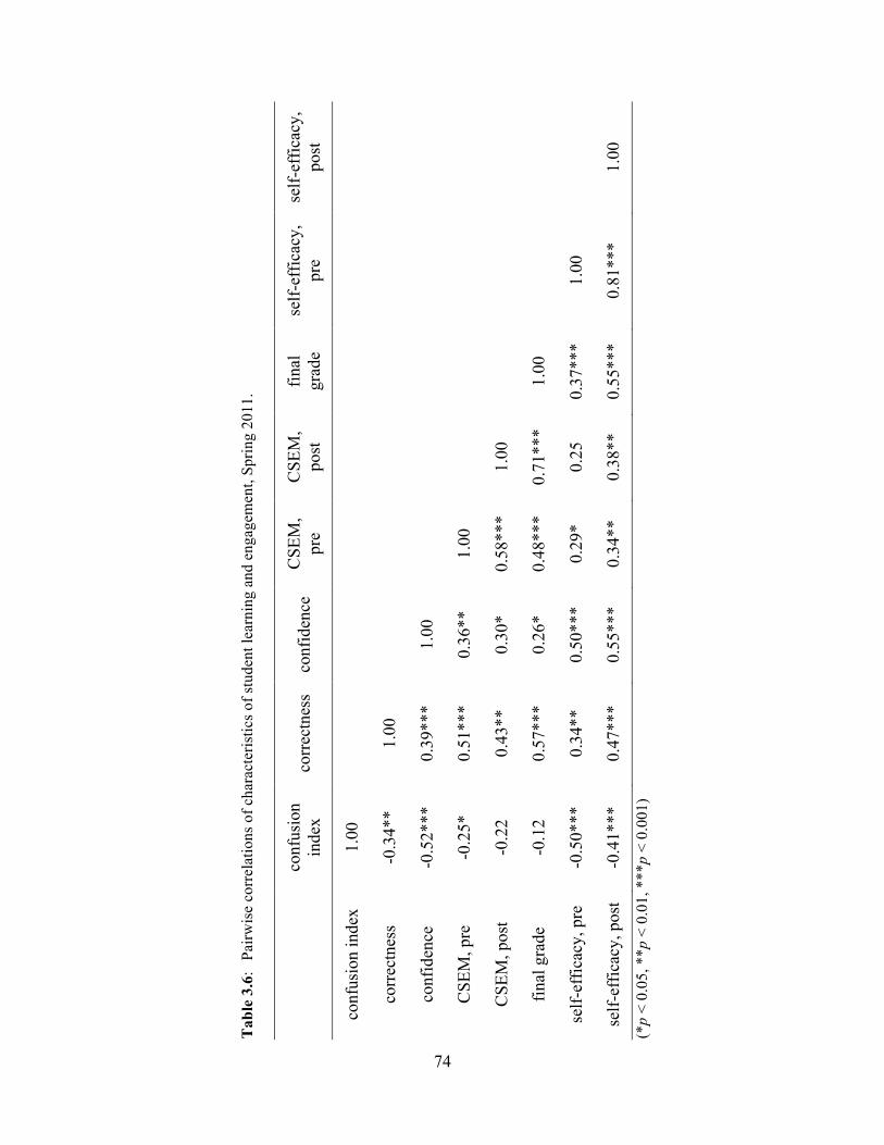
74
able 3.6: Pairwise correlation s of characteristics of student learning and engagement, Spring 2011.
74
Tab
le 3
.6:
Pairw
ise
corr
elat
ions
of c
hara
cter
istic
s of s
tude
nt le
arni
ng a
nd e
ngag
emen
t, Sp
ring
2011
.
co
nfus
ion
inde
x co
rrec
tnes
s co
nfid
ence
C
SEM
, pr
e C
SEM
, po
st
final
gr
ade
self-
effic
acy,
pr
e se
lf-ef
ficac
y,
post
conf
usio
n in
dex
1.00
corr
ectn
ess
-0.3
4**
1.00
conf
iden
ce
-0.5
2***
0.
39**
* 1.
00
CSE
M, p
re
-0.2
5*
0.51
***
0.36
**
1.00
CSE
M, p
ost
-0.2
2 0.
43**
0.
30*
0.58
***
1.00
final
gra
de
-0.1
2 0.
57**
* 0.
26*
0.48
***
0.71
***
1.00
self-
effic
acy,
pre
-0
.50*
**
0.34
**
0.50
***
0.29
* 0.
25
0.37
***
1.00
self-
effic
acy,
pos
t -0
.41*
**
0.47
***
0.55
***
0.34
**
0.38
**
0.55
***
0.81
***
1.00
(*
p <
0.05
, **p
< 0
.01,
***
p <
0.00
1)

75
Regression Analysis
To explore the interactions among these characteristics simultaneously, we build a series of
multiple regression models. As the primary goal of this analysis is to better understand what
student expressions of confusion tell us, we treat confusion (“confusion index”) as the outcome
variable in the models presented below. Although final grade may seem like a more natural
outcome variable because it is also an outcome of the course, merely including confusion as a
covariate does not adequately convey how it relates to other variables in the model.
Although we can build regression models in which both pre-test and post-test surveys are
included, the strong relationship between the two rounds of surveys renders one or both of them
statistically insignificant; we find this to be true of the FCI in the fall and of the CSEM and self-
efficacy survey in the spring. Thus, we consider only pre-tests of each survey in our regression
models.8
Table 3.7 and Table 3.8 summarize the most revealing regression models from the fall and
spring semesters, respectively. Standard coefficients are displayed. When only expression of
confusion and reading exercise correctness are included in the model (models 1f and 1s), there is
a statistically significant negative relationship between the two variables; in other words, when
no other variables are included in the model, an increase in correctness of one standard deviation
is associated with a decrease in confusion of approximately 0.25 standard deviations during the
fall semester and 0.34 standard deviations in the spring semester. However, only 6.2% and
11.7% of the variation in confusion is explained by correctness in the fall and spring semesters,
respectively.
8 The pre-test is more useful than the post-test as a covariate because it allows us to interpret the multiple regression analysis as a predictive model.

76
Table 3.7: Fitted linear regression models predicting expression of confusion by selected variables of student learning and engagement, Fall 2010.
variable model 1f model 2f model 3f model 4f
N 109 109 106 95
correctness -0.25** -0.12 -0.16 -0.05
confidence -0.37*** -0.41*** -0.37***
final grade 0.13 0.16
FCI, pre -0.29*
R2 0.062 0.185 0.208 0.247
RMSE 0.97 0.91 0.91 0.90 (*p < 0.05, **p < 0.01, ***p < 0.001)
Table 3.8: Fitted linear regression models predicting expression of confusion by selected variables of student learning and engagement, Spring 2011.
variable model 1s model 2s model 3s model 4s model 5s
N 90 90 89 88 72
correctness -0.34** -0.17 -0.28* -0.26* -0.26*
confidence -0.45*** -0.45*** -0.31** -0.34**
final grade 0.16 0.23* 0.37**
self-efficacy, pre -0.34** -0.41***
CSEM, pre -0.03
R2 0.117 0.289 0.317 0.401 0.496
RMSE 0.94 0.85 0.84 0.80 0.76 (*p < 0.05, **p < 0.01, ***p < 0.001)
When confidence in one’s explanation of the reading assignment is introduced into the model
(models 2f and 2s), the relationship between confusion and correctness is no longer statistically

77
significant. In other words, the negative relationship between confusion and correctness in
models 1f and 1s appears, in fact, to result from confusion and correctness both being strongly
related to confidence and only being weakly related to one another when confidence is held
constant. There is a strongly statistically significant negative relationship between confusion and
correctness during both semesters.
When final grade is introduced into the model (models 3f and 3s), it is not statistically
significant in either semester. However, interestingly, the relationship between confusion and
final grade is positive in this model. In the fall semester, neither correctness nor final grade is
statistically significantly related to confusion; only confidence is statistically significantly
related, and the relationship is strongly negative. In the spring semester, even though final grade
is not statistically significantly related to confusion, the introduction of final grade into the model
strengthens the negative relationship between correctness and confusion. So, in this case,
correctness and confidence are negatively related to expressions of confusion.
The next few models differ between the fall and spring semesters. In the fall (model 4f), FCI
pre-test performance is significantly negatively related to confusion, although its inclusion does
not qualitatively change the relationships among confusion, reading exercise correctness and
final grade. In the spring (model 4s), student pre-semester self-efficacy is introduced. When self-
efficacy is considered alongside final grade, confidence and reading exercise correctness, all four
of the variables are statistically significantly related to confusion. Perhaps most interestingly,
final grade remains positively related with expressions of confusion; an increase in score of one
standard deviation on the final exam is associated with an increase of 0.23 standard deviations of
confusion. Model 5s is included only to show that these relationships persist even when

78
controlling for CSEM pre-test performance; one might believe that controlling for students’
background knowledge could alter these relationships, but model 5s indicates that this is not so.
To better illustrate these relationships, in Figure 3.3 we highlight models 3f, 3s and 4s
described above. These three models are shown in different colors. Because each variable is
represented as a standard score, all of the variables may be represented on the same scale.
Figure 3.3: Fitted linear regression models predicting expression of confusion by selected variables of
student learning and engagement. Models 3f, 3s and 4s are displayed here. Each color represents a different model. The bars represent the 95% confidence interval around each of the mean values; if the confidence interval does not include the “zero line,” then the difference is statistically significant at the 0.05-level.
We see that the relationship between confusion and final grade is positive in all of these models ,
while the relationships between confusion and each of the other variables are negative. The same

79
relationships hold true in models 4f and 5s, which are shown in Table 3.8 and Table 3.9,
respectively; they are omitted from Figure 3.3 for simplicity.
Figure 3.4: Expression of confusion regressed against reading assignment correctness. Model 4s is
displayed in this prototypical plot of average confusion index against reading assignment correctness at final grades of A, B, C and D, using native units (rather than standard scores). These lines represent the fit to actual data; the data are not displayed here.
To further highlight the relationships between confusion and the two performance measures –
final grade and reading exercise correctness – from model 4s, we display a series of linear
regression lines relating confusion and correctness that are associated with a range of associated
final grades in Figure 3.4. In this case, we are no longer using standard scores; the plot area
ranges from “not at all” confused (0) to “somewhat” confused (1) on the vertical axis and from
“0 out of 2” to “2 out of 2” on the horizontal axis. Students of approximately the same level of
80
initial performance, confidence and self-efficacy who express more confusion tend to also
perform better than students who express less confusion. We do not observe any interaction
effects among the variables considered in this model.
Altogether, these variables explain 40.1% of the variation in confusion during the spring
semester; when CSEM performance is included, as shown in model 5s, the model actually
explains 49.6%. In the fall, however, the variables explain only 24.7% of the variation in
confusion. The rest of the variation may be noise, or representative of other dimensions of
student affect and performance that are not captured by the covariates presented here.
3.8 Discussion – Full Study
In averaging student expressions of confusion, confidence and correctness on reading exercises
over the semester, we effectively neutralize the effects of the spurious alternative hypotheses that
hindered the pilot analysis. Fortunately, we did not neutralize the main effects that we were
interested in studying.
The negative relationship between expressions of confusion and correctness on reading
exercises (models 1f and 1s) is contrary to the relationship suggested by our pilot analysis.
However, this finding is not necessarily surprising when we consider the large amount of
variation in expressions of confusion that is not explained by reading exercise performance; the
variables are related, but not very strongly. We note that, of the 43 reading exercises from both
semesters, 10 of them exhibit positive correlations between students’ expressions of confusion
and reading exercise performance. Therefore, it is possible that there are no fundamental
differences between the pilot analysis and the full study, and statistical fluctuations account for
the seeming discrepancy. On the other hand, as discussed in Section 3.5.2, there are several

81
alternative explanations for the observed pattern in the pilot analysis that cast doubt on whether it
reflects the relationship of interest. Either way, we have no reason to doubt the validity of the
relationship observed in the full study.
When final grade, confidence and self-efficacy are considered alongside reading assignment
correctness, we find that confusion is associated with both positive and negative course
outcomes. The suggestion of Crouch and Mazur (C. Crouch, 2000) that students who express
confusion about the content also tend to outperform others on the reading exercises is not
supported by these observations. However, the more nuanced notion that students who express
more confusion also tend to perform better in the end, assuming we control for other relevant
factors, is supported by these observations. Thus, we cannot claim that confusion is exclusively
good or bad; rather, we make two claims:
(1) When relevant factors are not controlled for, expressions of confusion are either
negatively-related or unrelated to reading exercise performance, confidence, final grade
and self-efficacy. Thus, expressions of confusion may be “bad,” or merely uninformative.
(2) When relevant factors are controlled for, expressions of confusion are negatively-related
to reading exercise performance, confidence and self-efficacy but positively-related to
final grades. Thus, assuming that we are interested in predicting final grades and
therefore controlling for other variables, confusion is “good.”
In other words, we are able to identify “productive confusion,” or the productive role of
confusion, but it is mixed with other, unproductive types of confusion in such a way that one
cannot isolate it without collecting additional information from students. We will discuss the
implications of these findings for instructors below.
82
In our discussion of self-efficacy, self-concept, metacognition and the role of confidence as a
means of probing these various theoretical elements of student engagement, we struggled to
establish which constructs are interchangeable and which constructs are distinct. In addition to
exploring the relationship between confusion and correctness, our present empirical efforts may
shed some light on the practical distinctions between these theoretical ideas.
3.8.1 Metacognition, Confidence and Self-Efficacy
The multiple regression analyses presented above suggest that the three probes of self-regulated
learning employed here – expressions of confusion, ratings of confidence, and evaluation of
physics self-efficacy – are distinct means of probing student engagement. Perhaps this is
surprising, as researchers have used confidence as a proxy for self-efficacy in previous studies
(Andrew, 1998). We find that students’ physics self-efficacy, expressions of confusion, and
confidence in their explanations are among the most highly-correlated factors considered in this
study, but the correlations, displayed in Tables 3.6 and 3.7, range from 0.4-0.6; none of the
factors are close to being co-linear. Thus, either the underlying constructs assessed by each of
these factors are different, or the various means of assessment – the different questions, contexts,
etc. – lead students to reply in different ways.
Ultimately, a theoretical framework that suppresses the subtleties that arise from the interplay
of these factors is not sufficient for describing this system. As our results show, the models only
explain a fraction of the variation in student expressions of confusion, and many of the
relationships change – or even reverse – when additional parameters are introduced. However,
while we claim that a robust theoretical framework should not collapse confidence, self-efficacy
and confusion together as a representation of metacognition, we cannot associate the variables

83
measured in this study with clear theoretical counterparts. One might argue that our probe of
self-efficacy is more akin to a probe of students’ “self-concept” (Linnenbrink & Pintrich, 2003;
Pietsch et al., 2003) because it is an assessment of students’ general beliefs in their abilities
rather than their beliefs in their ability to carry out specific skills, but such arguments require the
development of much more extensive, theory-focused research inquiries.
3.8.2 Changing the System by Measuring
We acknowledge that the act of asking students to participate in so many “metacognitive
activities” throughout the year could certainly change their behavior. We do not know, for
example, the extent to which confidence and performance are positively related simply because
students were asked about their confidence.
JiTT and PI are designed to make physics instruction more metacognitive. Frequent
opportunities for reflection about sources of confusion, coupled with collaborative interactions in
the classroom and a strong focus on the value of self-directed learning, are built on the
assumption that learning outcomes benefit from such activities. We note that, despite the much
more prominent role of lecture during the fall semester, the relationships observed across both
semesters are qualitatively similar.
In spite of all the metacognitive exercises, the average self-efficacy score of students in the
course virtually did not change over the duration of the spring semester (Table 3.5). This is
somewhat surprising, as we might have expected to observe some positive changes.

84
3.8.3 Implications for Instruction
There are two distinct questions about confusion that are particularly relevant to instruction: (1)
should we assess students’ expressions of confusion, and (2) how do we interpret students’
expressions of confusion? The answers to these questions depend on the manner in which
confusion is assessed.
When relevant factors are not controlled for, expressions of confusion are either negatively-
related or unrelated to reading exercise performance, confidence, final grade and self-efficacy.
Thus, if instructors assess expressions of confusion in such a way that they are unable to control
for the factors considered in this study, then “the less confusion, the better.” However, given that
the relationship between course outcomes and expressions of confusion is so weak, the best
advice may be simply to avoid assessing expressions of confusion in such an uncontrolled way.
On the other hand, when relevant factors are controlled for, expressions of confusion are
negatively-related to reading exercise performance, confidence and self-efficacy but positively-
related to final grades. Thus, if instructors assess confusion in such a way that they can control
for these negatively-related factors, such as the means of assessing confusion that is presented
here, then they can distill the productive role of confusion from the unproductive roles.
Monitoring the productive role of confusion affords instructors the opportunity to both assess
students’ metacognition as they engage in activities and perhaps even promote such constructive
expressions of confusion.
Ultimately, expressions of confusion, when carefully assessed, can play a positive, important
role in instruction.

85
3.8.4 Limitations
We note several specific limitations of this study.
Asking students to express their confusion before responding to content-related questions
could introduce a stereotype threat that affects performance. This effect would induce a negative
relationship between confusion and correctness, which is precisely what we observed; we cannot
determine the extent to which this stereotype threat may be amplifying the negative relationship.
Ironically, the confusion question was posed before the other questions because we did not want
to introduce bias in the other direction; that is, we did not want to influence students’ responses
about their confusion by asking them challenging questions about the reading assignment
immediately beforehand. We were also concerned that students would say, “I am confused about
the previous question,” rather than something related to the reading (in the fourth “follow-up”
question, many students responded in precisely that way).
Another limitation of our analysis is that we depend upon students to rate their confidence,
confusion and physics self-efficacy on scales that are not calibrated to any external standards.
One student may interpret his/her abilities and understandings very differently than another
student who, objectively, may be very similar. In addition to the potential disconnect between
what students think and what they express, this lack of calibration introduces another potential
disconnect between what students express and what they mean to express. Ideally, we would
develop calibration activities that students could use to gauge their own responses, but we are
also very conscious of the low tolerance students have for inconveniences. When more work is
required to complete the assignment, the likelihood that students will skip the introspection
process increases. Perhaps descriptive rubrics or sample responses would help, though such
materials may bias responses of students.

86
3.8.5 Future Directions
The relationship between expressions of confusion and student reasoning, not merely
correctness, could be much more revealing. As we have this data already, one potential direction
of future research involves analyzing students’ explanations to investigate how these relate to
expressions of confusion. Furthermore, the free-response data collected here can be used to
inform and redesign the multiple-choice component of the questions posed over the course of
this study. From this data set, we can also identify particular students – high-performing students
who express slight confusion, low-performing students who express much confusion, etc. – and
investigate their free-response data to better understand confusion as a form of assessment.
From a more theoretical point of view, now that we observe students’ distinct responses to
separate measures of confidence, confusion, and self-efficacy, we are able to explore the ways in
which each of these measures relates to the theoretical constructs of self-concept, self-efficacy,
metacognition, motivation, identity, and numerous other components of the theories described in
Section 3.2. Perhaps we must consider the possibility that self-efficacy, like knowledge (diSessa,
2006), exists in pieces and may or may not be activated in different contexts.
Finally, from a more practical point of view, now that we observe a productive role of
confusion in instruction, we may be able to further explore the causal relationships between this
kind of confusion and course outcomes. Additionally, we may be able to explore the relationship
between changes in expressions of confusion, as well as changes in the productiveness of
confusion, to specific activities in class.

87
3.9 Conclusion
Students who express more confusion tend to also express lower confidence, lower self-efficacy,
and, to a slight degree, weaker performance on reading exercises. However, when we control for
all of these factors, students who express confusion tend to also perform better overall, as
measured by final grade. Thus, we suggest that, when relevant factors are not controlled for,
expressions of confusion may be either bad or merely uninformative; but when relevant factors
are controlled for, assuming that we are interested in relating assessment of confusion to final
grades, confusion is good. In other words, we are able to identify and isolate the productive role
of confusion using surveys and reading assignment activities that are entirely accessible to
instructors. Thus, if instructors assess confusion as presented here, then they can monitor the
productive role of confusion, assess students’ metacognition as they engage in activities, and
perhaps even find ways to promote such constructive expressions of confusion.

88
Chapter Four
Exploring “Design” in the Introductory
Physics Laboratory
The introductory physics laboratory, sometimes treated as an appendage to the primary
physics course, actually plays a very important role in physics education. Many of the
activities that students undertake and the skills that they learn are (1) essential to a well-
rounded understanding of the theory and practice of physics and (2) primarily accessible and
assessable in the laboratory setting (Singer et al., 2006). Therefore, we explore this
dimension of student learning and engagement by investigating students’ exhibition of
scientific reasoning and data handling skills in laboratory activities designed with different
89
degrees and means of scaffolding inquiry. Our goal is to compare each of these approaches to
inquiry, which are described in detail below, to one another and to compare both approaches
to other institutions where comparably structured inquiry-based laboratory activities are
implemented. We observe slight differences between the groups, and we find that even some
of the most strongly-emphasized skills are either not exhibited or not retained by many of the
students.
4.1 Introduction
Traditional laboratory exercises often involve carrying out a specified procedure, measuring
some physical parameters, and performing quantitative analysis. The intent is usually to provide
“hands-on” experience in science to students, reinforce the rules and relationships presented in
lecture, and convey a sense that science is cool. Other potential goals, such as clarifying the
scientific method and improving student understanding of measurement, error, and assumptions,
are often not articulated and largely neglected during instruction.
Therefore, we assess how different strategies in laboratory instruction impact the
achievement of various learning and skill development goals.
4.2 Background
As this study is focused on the redesign and implementation of two pedagogical approaches, we
begin by motivating such changes from a goal-oriented perspective. We discuss previous
research in the design of instructional laboratories. To better contextualize our results, we
consider several theories related to transfer of knowledge. Transfer is important because, once
we establish that laboratory activities should focus on scientific reasoning skills, the variations in

90
content from one lab to the next are actually just changes in context. Thus, we must have a
productive model of transfer to understand our observations.
4.2.1 Learning Goals in the Laboratory
Reif and St. John find that students are unable to articulate the central goal of an experiment, its
underlying theory, or its basic methods in “traditional” laboratory classes where laboratory
activities are not built around goals and goals are not clearly articulated to students (F. Reif &
John, 1979). Subsequent studies have reinforced this finding (Domelen & Heuvelen, 2002;
Richard R. Hake, 1992; Patricia Heller & Hollabaugh, 1992; Patricia Heller, Keith, & Anderson,
1992; Hofstein & Lunetta, 1982; Redish, Saul, & Steinberg, 1997; Redish et al., 1998; F. Reif &
Reif, 1987; Wells et al., 2008). All of these studies involved the identification of learning goals.
Welzel and colleagues collected survey responses from hundreds of laboratory instructors and
summarized results in the following goal categories (Welzel et al., 1998):
(1) for the student to link theory and practice;
(2) for the student to learn experimental skills;
(3) for the student to get to know the methods of scientific thinking;
(4) for the student to foster motivation, personal development and social competency; and
(5) for the teacher to evaluate the knowledge of the student.
These general categories provide a framework for discussing the different goals emphasized by
science education researchers in other settings. “Traditional” laboratories focus largely on the
first and second goal categories, even though specific goals are not always made explicit.

91
Scientific Community Laboratories
Scientific Community Laboratories (SCLs), developed at the University of Maryland, are
designed to teach students how to produce, analyze and evaluate scientific evidence (Kung,
2005; Lippmann, 2003). This goal is encapsulated by the second and third categories listed here.
The printed materials that are distributed to students include a very brief description – perhaps
one short paragraph – of the phenomenon under consideration, one primary question, and a
timetable describing how much time students should devote to each stage of the process.9
Students are expected to investigate the primary question using materials that are available.
Class-wide discussions take place between stages of planning, data collection, analysis and
reporting. In reporting on the effectiveness of these laboratories, Lippmann Kung reports that
students struggle with the idea of measurement, particularly when it’s related to uncertainty
(Kung, 2005).
ISLE Design Laboratories
Etkina and colleagues have developed and implemented the investigative science learning
environment (ISLE) instructional design laboratories (Etkina et al., 2010). The printed materials
that are distributed to students include a statement of learning goals, a series of experimental
inquiries, and descriptions of the scientific abilities upon which these activities focus.10 Each
inquiry – experiment, investigation, question, etc. – is followed by a series of steps that guide
students through the inquiry process. Etkina and colleagues define very specific criteria for
evaluating student understanding of uncertainty and scientific assumptions (among other 9 More information and complete SCLs are available here: http://umdperg.pbworks.com/w/page/10511229/Scientific%20Community%20Labs 10 More information and complete ISLE design laboratories are available here: http://paer.rutgers.edu/ScientificAbilities/Design+Experiments/default.aspx

92
scientific abilities). They find that students do not “saturate” these scientific abilities after one
semester of instruction (Etkina et al., 2008). Additionally, they report that design laboratories are
not as effective without strong scaffolding – reflection, historical reading passages, and rubrics –
and non-design laboratories are even less effective. These findings support the notion that
scientific abilities are not trivially linked to the laboratory setting.
Summary
While all of these novel designs, as well as the associated evaluation measures, appear to be very
effective at improving scientific abilities in the laboratory, there are still unanswered questions.
Both SCLs and design laboratories focus on developing scientific skills and abilities, but are not
optimized to maximize physics content. This is not to say that these laboratories do not include
physics content; rather, instead of spending more time on addressing sophisticated material, they
allow for more emphasis on design and inquiry.
Depending on the goals of the laboratories in an introductory science course, the optimal
strategy for laboratory design and implementation may vary. We assert that the primary goal of
the laboratory is to enhance scientific reasoning skills, primarily because this is an important
goal and the student laboratory is the only component of the introductory physics course where
such a goal is possible. In this case, the optimal strategy may involve less emphasis on advanced
content and more emphasis on scientific abilities.
4.2.2 Degree of Guidance
Hand-in-hand with the discussion of laboratory goals is the discussion of the degree of guidance
that an instructor provides to students. If content-oriented goals require students to have a
93
sophisticated understanding of the material, time constraints may necessitate stronger guidance
in the content and design of the laboratory. However, strong guidance may not be associated
with the most effective learning.
Through an investigation of student engagement using Physics Education Technology
(PhET) simulations, Wieman and Adams observed that limited guidance is superior to stronger
guidance for student engagement, as measured by monitoring the extent to which students
explored PhET simulations and the number of questions students asked the moderator as they
worked (Wendy K Adams, Paulson, & Wieman, 2008). They identify four degrees of guidance:
“no instruction,” in which students are asked to play with the simulation and talk out loud as they
try things; “driving questions,” in which simulation work is preceded by some relevant general
conceptual questions; “gently guided,” in which the simulation work is accompanied by specific
questions that are related to the activity; and “strongly guided,” in which the activity is dictated
in step-by-step format. They suggest that the “no instruction” and “driving questions” strategies
allow students to form and investigate their own questions, and thus more effectively build from
their own understanding of the material. Wieman and Adams point out that “no instruction” fails,
however, if the simulation is too complex or poorly designed.
Even without additional questions, the simulations themselves implicitly provide guidance.
Although the study described here relates to physics simulation activities, the interactive, self-
directed approach to learning is analogous to the laboratory environment. The laboratory setting
is inherently more complex, and the environment contains inherently less guidance, suggesting
that students are more likely to fail to engage without some degree of scaffolding.
94
Scaffolding
Holton and Clark describe scaffolding, a general term that includes the elements we consider
“degrees of guidance,” in relation to metacognition and social activities involved in learning
(Holton & Clarke, 2006). They identify three types of scaffolding – expert scaffolding, reciprocal
scaffolding and self-scaffolding, which is equivalent to metacognition – and two scaffolding
domains: conceptual and heuristic.
Conceptual scaffolding targets conceptual development, whereas heuristic scaffolding
attempts to transcend specific content to promote heuristics for learning and problem solving. In
describing metacognition, Schraw and colleagues describe heuristic scaffolding in different
terms, instead referring to declarative, procedural and conditional knowledge of cognition
(Schraw et al., 2006).
SCLs, introduced above, contain very limited scaffolding on paper; ISLE design laboratory
exercises, in contrast, contain extensive heuristic scaffolding and very limited conceptual
scaffolding. However, both approaches to the laboratory contain many opportunities for
discussion among peers and with instructors, which is intended to play a heuristic (rather than
conceptual) role.
4.2.3 Transfer
The importance of the ability to transfer skills and knowledge from one domain to another plays
a role in virtually all of the theoretical frameworks discussed in previous chapters. In discussing
self-efficacy, Bandura comments that experiences of success are more likely to affect personal
efficacy when threats are mastered in various circumstances (Bandura, 1977). Georghiades
suggests that metacognition may mediate improvement of transfer and durability of scientific

95
conceptions in the framework of conceptual change (Georghiades, 2000). The process of
conceptual change is not complete unless there is evidence that the newly-changed concepts can
be transferred to different contexts; the decay of conceptual change over time from an inability to
transfer skills and concepts is, therefore, a central problem in education. Georghiades argues that
transfer is not synonymous with “application” because application is only part of the process of
transfer; before applying, one must recognize that the knowledge can transfer, determine which
elements change and which elements do not change and then test applicability. In linking transfer
to teaching practices, Georghiades highlights metacognition, and specifically metacognitive
activities together with social activities, as a way of overcoming the decay in conceptual change
(Georghiades, 2000).
Challenges to Classical Transfer Theory
Broadly speaking, classical transfer theory refers to the association of common elements from
one context to another; the notion of what constitutes an “element” has evolved with the
development of theories of cognition, but the underlying principle remains. Georghiades’
characterization of transfer is slightly different than the classical transfer theory. He treats
transfer and learning as largely synonymous, in that a failure to transfer is essentially a failure of
conceptual change. However, this fusion of transfer and learning actually side-steps fundamental
flaws in the classical treatment of transfer (Lobato, 2006). Challenges to the classical theory stem
from the potentially unique ways in which individuals detect similarities across situations and the
importance of distinguishing between superficial and deep, structural elements. Lobato, citing
others, highlights five theoretical problems with the classical transfer approach (Lobato, 2006):11
11 Items are enumerated here for clarity; the quoted passage appears in paragraph form in the original publication.

96
(1) Classical transfer studies privilege the perspective of the observer and rely on models of expert performance, accepting as evidence of transfer only specific correspondences defined a priori as being the “right” mappings (Lobato, 2003; Seeger & Waschescio, 1998). […]
(2) At the root of the transfer problem is a functionalist view of knowledge in which “the beneficial cognitive consequences of decontextualized learning, freeing oneself from experience” are seen as “a condition for generalization about experience” (Lave, 1988, p. 41). […]
(3) According to critics, transfer researchers often interpret context as task presented to students and analyze the structure of tasks independently of students’ purposes and construction of meaning in situations (Carraher & Schliemann, 2002; Cobb & Bowers, 1999; Greeno, 1997).
(4) The “applying the knowledge” metaphor of transfer suggests that knowledge is theoretically separable from the situations in which it is developed or used, rather than a function of activity, social interactions, culture, history and context. […]
(5) The static nature of the application or transportation metaphor suggests that “the formation of transfer environments is not assumed to be an actual part of the process, but rather is seen as differentially supporting or interfering with it” (Tuomi-Gröhn & Engeström, 2003, p. 40). (p. 434)
Some researchers address the challenges and shortcomings by distinguishing between
different kinds of transfer. Perkins and Salomon consider transfer as they shift from discussing
“expertise” as a general quality towards context- and content-specific expertise (Perkins &
Salomon, 1989). They suggest that people fail at “transfer tasks” because they are too good at
transfer and apply too much from the familiar situations to new situations. They modify classical
transfer theory by introducing two kinds of transfer: the “low road” to transfer, which depends on
extensive and varied practice, and the “high road” to transfer, which depends on deliberate
abstraction of a principle. McKeachie suggests that, in some situations, low-road, automatic
processes are more productive than high-road, metacognitive processes when the latter interfere
with the former (McKeachie, 1987).
97
However, such distinctions do not address the problems with classical theory because
transfer is still treated as an unproblematic construct where the only challenge is facilitating its
occurrence (Lobato, 2006). Classical transfer theory suffers from the fact that there is little
agreement about what transfer actually means (Barnett & Ceci, 2002).
Alternatives to Classical Transfer Theory
Some believe that transfer is fundamentally flawed as a research construct because we must
either (1) reject the notion of transfer, and therefore also reject constructivism, or (2) accept the
notion of transfer, and also accept some vague ideas about how knowledge, abstraction and
context are conceived (Carraher & Schliemann, 2002). Abstraction seems at odds with theories
of contextualized learning unless researchers adopt a different view of abstraction (Lobato,
2006). Several alternative conceptions of abstraction stem from reflective abstraction (Jean
Piaget, 1980), described as “a constructive process in which the regularities abstracted by the
learner are not inherent to the situation, but rather are a result of personal structuring related to
the learner’s goals and prior knowledge” (Lobato, 2006, p. 441).
Lobato’s alternative to classical transfer theory is actor-oriented transfer. From the actor-
oriented perspective, the focus shifts from the instructor’s viewpoint to the student’s viewpoint
(Lobato, 2003). The goal is to understand how learners generate – or fail to generate – their own
similarities between problems. This shift in focus modifies the criteria for evidence of transfer;
whereas classical transfer theory considers strong performance in a different task to be evidence
of transfer, the actor-oriented perspective considers the act of drawing similarities between new
situations and previous experiences evidence of transfer.

98
Lobato also discusses mechanisms of transfer (Lobato, 2006). Such mechanisms include
“focusing phenomena,” features in a classroom environment that direct students’ attention
toward certain properties or patterns, and “social framing,” a way of framing both activities and
students’ roles as being connected with other contexts in which the learning experiences are
relevant, and “discernment of differences,” in which students consider differences between
situations to ultimately refine transfer ability.
4.3 Methods
Transfer effectively characterizes the learning that takes place in the introductory physics
laboratory because each activity is a different means of encountering and building on the same
underlying set of skills. Students may encounter new concepts and engage with content that is
still somewhat unfamiliar, but the scientific reasoning skills are reinforced in every session in
different contexts. Regardless of how well defined the theoretical framework for describing such
transfer of skills is, students must be able to translate experiences from one context to another in
order to be successful in the laboratory. Moreover, instructors must be able to assess this transfer.
This study investigates student exhibition of scientific abilities in the instructional laboratory
setting. We approach this analysis through the lens of the instructor, who cannot scrutinize
video-recorded discussions and activities for evidence of sense-making and critical thinking.
Although such methods are invaluable research tools and could provide insight into this subject,
logistical constraints prevented us from conducting such discourse analysis in this investigation.

99
4.3.1 Course Information
We analyzed data collected in the second semester of a two-semester sequence of introductory
physics courses at Harvard University during the spring of 2011. This course focused on topics
related to electricity and magnetism and was designed for non-physics concentrators. As
described in Chapter Three, the instructor employed Peer Instruction (PI); demonstrations were
used in conjunction with in-class conceptual questions and discussion, and lecture was limited.
Figure 4.1: Dual sequences of introductory laboratory activities. The two sequences, involving ISLE
design labs (heuristically scaffolded, inquiry-based activities) and SCLs (exploratory, virtually no formal scaffolding) after an initial traditional lab (heavily scaffolded, both heuristically and conceptually) are displayed here. Blue and green arrows, respectively, represent the two sequences.
The laboratory component of the course involved five bi-weekly – i.e., meeting on
alternating weeks – sessions over the duration of the semester. Laboratory activities were related
to content that was being discussed concurrently in the classroom and recitation sections. Each

100
student enrolled in one of six laboratory sections, and each section took place at a different time.
The sequences of laboratory activities were designed as follows: the first session was relatively
traditional, with explicit procedures and step-by-step instructions; the second session was closely
modeled after the design labs developed for ISLE, with extensive heuristic scaffolding but very
limited conceptual scaffolding; the third and fourth sessions were split so that activities closely
modeled after the ISLE design labs were carried out in three sections and activities closely
modeled after SCLs, which were largely exploratory with virtually no formal scaffolding, were
carried out in the other three sections; and the fifth session was modeled after SCLs. These
sequences are illustrated in Figure 4.1.
After enrollment, we determined which laboratory sections would receive which sequence of
activities based on two criteria: (1) the number of students participating in each sequence should
be approximately equal to one another and (2) more scaffolded activities should take place after
less scaffolded activities whenever possible. Students were permitted to attend a different section
if they had a conflict with their regular section before the third meeting (i.e., before the split);
however, students were required to continue attending the same section once different sequences
were established.
No pre-laboratory exercises were assigned, and reports were always submitted at the end of
the three-hour session. These reports included a statement of purpose, hypothesis and
predictions, experimental procedure, collected data, analysis of collected data and conclusions.
Students worked in groups of two, three or four students and submitted laboratory reports as a
group. Students were not required to form the same group each week. They were encouraged to
work diligently throughout the session but not to worry if they did not finish the exercises, since
they would be evaluated on the quality of the report rather than the number of activities they

101
completed. Rubrics developed for use with Design Labs were used to evaluate reports. All of the
printed laboratory activities are included in Appendix B, and the complete set of rubrics is
included in Appendix C.
Graduate student assistants facilitated the laboratory sections with the help of the laboratory
preceptor.12 The laboratory assistants meet weekly with the project management team to learn
about the goals and objectives for the laboratory and carry out the experiments themselves.
4.3.2 Measures
This is a mixed-methods study in which we analyzed both quantitative and qualitative data.
Quantitative measures included pre- and post-course performance on the Conceptual Survey of
Electricity and Magnetism (CSEM) and the Data Handling Diagnostic (DHD), performance on
course-related activities (problem sets, laboratory activities, exams and cumulative grades), and
rubric-based assessment of exhibition of scientific reasoning abilities in laboratory reports.
Additionally, we analyzed pre- and post-course performance on a survey of self-efficacy in
physics. Qualitative measures include the summative analysis of students’ exhibition of specific
scientific reasoning skills over the duration of the semester.
Conceptual Surveys
The CSEM was administered to assess students’ conceptual understanding of electrostatics and
magnetostatics (Maloney et al., 2001). The survey consists of 32 multiple-choice questions that
are designed to elicit students’ intuitive ways of thinking – which may or may not be correct – 12 We note that most of the exploratory activities were under the supervision of one graduate assistant and most of the scaffolded activities were under the supervision of another graduate assistant. A third graduate assistant supervised both laboratories. Although the optimal arrangement would have involved all three assistants in both sequences, we find that results of our analysis persist even when we control for graduate assistant. The laboratory preceptor co-supervised all laboratory sections.

102
through the use of “everyday” language instead of terminology typical of the physics classroom
and response choices that appeal to empirically-identified incorrect ways of reasoning.
The DHD was administered to assess students’ data handling abilities. The survey, consisting
of 23 multiple-choice questions, was developed by researchers and instructors at the University
of Edinburgh to better understand challenges that students encounter when analyzing and
interpreting collected data (Galloway et al., in press). Unlike the FCI and CSEM, the DHD does
not avoid language that is typical of these kinds of problems; the goal is not necessarily to evoke
a particular way of thinking about the problems, but rather merely to assess student performance
on the items.
Both surveys were administered as a pre-course assessment during the first week of the
semester and as a post-course assessment sometime after the final class meeting and before the
final exam. Both surveys were administered using the Internet-based Interactive Learning
Toolkit; students had 45 minutes to complete each survey. They received credit for participation,
but not for correctness.13
Course-Related Performance
If we were to include all of the criteria representing various aspects of students’ performance on
course-related activities in our analysis, many of the factors would be redundant. Therefore, we
employ the statistical technique of factor analysis to determine if the correlations among
different variables actually describe one or more uncorrelated aspects of performance (Costello
& Osborne, 2005). 13 Based on our analysis in Chapter Two, perhaps we could treat these conceptual surveys as categorical variables. Indeed, this approach has been done by others (Watkins, 2010). However, in our analysis, we are primarily interested in examining students’ pre-course performance, in which there are no ceiling effects. Therefore, we are not inclined to complicate the interpretation of our analysis, while simultaneously suppressing potentially relevant information, if we do not need to do so.

103
We find that reading exercises (evaluated for participation only), laboratory activities, mid-
term exams, final exams and final grades all describe virtually one factor; the difference between
the first and second eigenvalues is much larger than the differences between subsequent
eigenvalues. The final exam and final grade are weighted most heavily in determining that factor.
Therefore, for simplicity and clarity, we choose to employ final grade as the primary summative
measure of students’ performance in the course.
Laboratory grade is not heavily weighted in the factor analysis described above; it is, in fact,
rather weak. Moreover, laboratory grades are very highly correlated with our own rubric-based
assessment (r = 0.78). Therefore, we do not include the “grading” assessment in our analysis and
focus on the instead on our own more rigorous, research-driven assessment of the submitted
reports.
Scientific Reasoning Abilities
We used the scientific ability rubrics developed for the ISLE curriculum to evaluate students’
laboratory reports (Etkina et al., 2006). Each ability is rated on a four-point scale, and each of the
four possible ratings includes an explicit statement of the type of student response that would
merit that rating. During analysis, we implement the rubrics exactly as they are implemented
with the ISLE courses at Rutgers University so that we are able to direct compare the exhibition
of scientific abilities among students in both sequences of this physics laboratory with previously
reported findings. Although there are many differences between the two contexts, the
measurement tool is kept constant.
Moreover, we implement these rubrics to ensure that students are evaluated upon their
exhibition of the skills of interest, and that students understand the criteria upon which they are

104
being evaluated. The rubrics employed for research assessment were also used for grading, and
they were provided to students with the laboratory activities.14,15 All of these materials are
included in Appendix B. Assessment for research purposes was conducted independently and
blinded from the grading of laboratories for course credit; the degree of rigor is much lower and
the time constraints are much higher in the latter case, whereas thoroughness and objectivity are
essential in the former case.
Specifically, fifteen scientific abilities were assessed for research purposes. These abilities
are summarized in Table 4.1. The ISLE labels correspond to where these abilities appear on the
full set of rubrics.
Most of the laboratory activities assess, explicitly or implicitly, all 15 of the scientific
reasoning abilities highlighted here; however, some of the activities simply do not require
students to exhibit certain abilities. As one might expect, students do not exhibit abilities that are
not required (e.g., evaluating uncertainty while conducting qualitative experiments). In such
instances, we do not assess students’ laboratory reports for exhibition of such abilities.
Specifically, we do not assess abilities B2/C2/D2, C4, and F1 in the first laboratory, ability G2 in
the fourth laboratory, and abilities C3, C4, and G3 in the fifth laboratory.
For some of the abilities displayed here, the rubrics are very specific – e.g., C8 refers to a
“testing” experiment in which a hypothesis is being tested and D4 refers to an “application”
experiment in which a particular problem is to be solved or measurement is to be made, but
otherwise the skills are very similar – so we collapse these rubrics and apply whichever one is
14 Students found the complete rubrics used for grading reports from the first three sessions overwhelming and unhelpful. Therefore, we provided less information to students in sessions four and five. 15 For research purposes, we are interested in the exhibition of several criteria over the course of the semester. Therefore, even though the rubrics used for grading vary over the semester and span many scientific abilities (as the laboratory activities reveal), only 15 specific scientific abilities are investigated here.

105
more sensible for assessment of a given laboratory activity. This is in keeping with how the
rubrics are used for research purposes in previous studies (Karelina, 2011).
Table 4.1: Scientific reasoning abilities. Students’ laboratory reports were assessed on the 15 scientific reasoning abilities shown here.
ISLE label Scientific Reasoning Ability
A3 Is able to evaluate the consistency of different representations and modify them when necessary
B2/C2/D2 Is able to design a reliable experiment
B7 Is able to identify a pattern in the data
B9 Is able to devise an explanation for an observed pattern
B10/C5/D8 Is able to identify the assumptions
C3 Is able to distinguish between a hypothesis and a prediction
C4 Is able to make a reasonable prediction based on a hypothesis
C6/D9 Is able to determine specifically the way in which assumptions might affect the prediction/results
C8/D4 Is able to make a judgment about the hypothesis/results of the experiment
F1 Is able to communicate the details of an experimental procedure clearly and completely
G1 Is able to identify sources of experimental uncertainty
G2 Is able to evaluate specifically how identified experimental uncertainties may affect the data
G3 Is able to describe how to minimize experimental uncertainty and actually do it
G4 Is able to record and represent data in a meaningful way
G5 Is able to analyze data appropriately

106
Self-Efficacy Survey
This survey, administered as a pre-test during the first week of classes on paper and as a post-test
between the last class and the final exam via the Internet, was designed to measure both
“physics” self-efficacy and “Peer Instruction” self-efficacy. It was based on a similar survey
designed to assess physics self-efficacy (Fencl & Scheel, 2004). Seven of the questions related
explicitly to students’ belief in their ability to perform physics-related activities, and eight of the
questions related explicitly to students’ belief in their ability to engage in Peer Instruction
activities. Students responded to questions on a Likert scale (five-point scale from strongly
disagree to strongly agree). Refer to Chapter Three for a much more detailed discussion of self-
efficacy.
Although this survey is not directly related to the research questions posed here, we
investigate the possibility that different experiences in the laboratory may have different effects
on students’ self-efficacy. The survey was implemented both to assess students’ physics self-
efficacy and to investigate whether students’ exhibit Peer Instruction self-efficacy. The latter is
the subject of ongoing research, so we only consider the first series of questions, related to
physics self-efficacy, in our analysis.
4.3.3 Sample Description
Data from 89 students were analyzed, though not all students completed all surveys; response
rate information is included in subsequent tables. Table 4.2 displays the descriptive statistics for
the CSEM, the DHD, course performance metrics and the physics self-efficacy survey. The mean
values of the DHD and physics self-efficacy survey change only slightly over the duration of the
semester. The mean CSEM increases from 12.76 to 21.95 on a scale of 0 to 32.

107
Table 4.2: Descriptive statistics of characteristics of student learning and engagement, Spring 2011.
variable N mean median s.d. range
CSEM, pre 72 12.76 12 5.73 2 – 27
CSEM, post 55 21.95 23 6.76 6 – 32
final exam 89 0.70 0.70 0.15 0.33 – 1.00
final grade 89 85.36 86.44 8.76 57.63 – 99.29
DHD, pre 74 12.11 12.5 2.73 4 – 18
DHD, post 53 12.68 13 2.65 6 – 18
self-efficacy, pre 88 3.51 3.57 0.73 1.14 – 5.00
self-efficacy, post 81 3.45 3.43 0.72 1.00 – 5.00
Table 4.3 displays the rating counts of the 15 scientific reasoning abilities highlighted in Table
4.1. These counts are cumulative, summed over the five laboratory activities that students carried
out during the semester. Some abilities were not assessed on certain laboratory activities.
Table 4.3: Exhibition of scientific reasoning abilities, Spring 2011. The cumulative rating counts, summed over the five laboratory activities, of each of the 15 scientific reasoning abilities of interest are shown here.
Ability 0 1 2 3
Is able to evaluate the consistency of different representations and modify them when necessary 0 3 47 81
Is able to design a reliable experiment 0 1 26 77
Is able to identify a pattern in the data 0 7 27 97
Is able to devise an explanation for an observed pattern 16 31 15 69
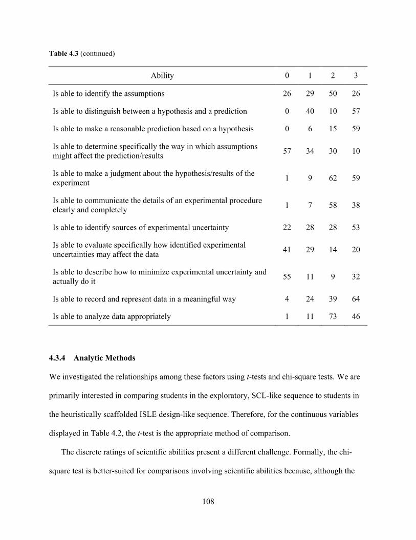
108
Table 4.3 (continued)
Ability 0 1 2 3
Is able to identify the assumptions 26 29 50 26
Is able to distinguish between a hypothesis and a prediction 0 40 10 57
Is able to make a reasonable prediction based on a hypothesis 0 6 15 59
Is able to determine specifically the way in which assumptions might affect the prediction/results 57 34 30 10
Is able to make a judgment about the hypothesis/results of the experiment 1 9 62 59
Is able to communicate the details of an experimental procedure clearly and completely 1 7 58 38
Is able to identify sources of experimental uncertainty 22 28 28 53
Is able to evaluate specifically how identified experimental uncertainties may affect the data 41 29 14 20
Is able to describe how to minimize experimental uncertainty and actually do it 55 11 9 32
Is able to record and represent data in a meaningful way 4 24 39 64
Is able to analyze data appropriately 1 11 73 46
4.3.4 Analytic Methods
We investigated the relationships among these factors using t-tests and chi-square tests. We are
primarily interested in comparing students in the exploratory, SCL-like sequence to students in
the heuristically scaffolded ISLE design-like sequence. Therefore, for the continuous variables
displayed in Table 4.2, the t-test is the appropriate method of comparison.
The discrete ratings of scientific abilities present a different challenge. Formally, the chi-
square test is better-suited for comparisons involving scientific abilities because, although the

109
ratings scale from zero to three, nothing about the ratings suggests that they should be exactly
one unit apart from one another. The different ratings might as well be represented by shapes or
colors instead of numbers. However, the chi-square test requires that the expected count in each
cell be at least five (Moore et al., 2008), which is not necessarily true. Therefore, we address the
problems by two means: (1) we assume that ratings are, in fact, one unit apart from one another
and employ t-tests and (2) we merge ratings that contain fewer than five counts with neighboring
ratings and employ chi-square tests. Both methods are reported below.16,17
We do not employ statistics in our analysis of changes in individual scientific reasoning
abilities over the duration of the semester. We would almost certainly measure some statistically
significant differences across the five sessions, but such differences are not as informative as the
objective, qualitative analysis of the time evolution of the exhibition of specific reasoning
abilities.
Two researchers independently coded students’ submitted laboratory reports and
subsequently discussed coding. All discrepancies were resolved during discussion, and the rubric
criteria were further defined to eliminate future discrepancies. Once the criteria were sufficiently
well established through discussion, remaining reports were coded independently. 16 We note that when we group all the students’ submitted reports together for analysis, we are counting multiple reports from the same individuals as independent data. Reports were submitted by groups of students, and these groups varied from session to session, but ultimately the same groups of students contributed reports on five distinct occasions. Because groups varied, we cannot calculate semester-long averages by groups of students. However, we also cannot assess each session independently because of the count requirements for chi-square analysis. Therefore, we cautiously acknowledge the potential for artificially improved statistical power, though we also highlight the variations between labs and between groups that may mitigate such effects. Also, as our results show, almost none of the comparisons reveal statistically significant differences. 17 We note that, in comparing so many scientific abilities, the likelihood of a spurious yet statistically significant difference is not negligible. The Bonferroni correction, which depresses the threshold for statistical significance when multiple comparisons are being analyzed, would help prevent this. However, as we shall see, virtually all of the comparisons are not significant (and the one comparison that is significant is very significant). Therefore, we acknowledge the correction technique but forgo discussion as it is not necessary in our analysis.

110
As mentioned, we employ factor analysis techniques to establish which course performance
measures should be used for analysis.
4.4 Results
The present analysis branches in two primary directions: (1) comparison of exploratory and
scaffolded laboratory sequences to one another and (2) investigation of the exhibition of
scientific reasoning abilities over the duration of the semester. These two branches are not
entirely separate from one another, as described below.
4.4.1 Comparison of Exploratory and Scaffolded Sequences
As the two sequences are distinct only after the second laboratory session, only laboratory
sessions three, four and five are considered in the following comparisons.18
Table 4.4 summarizes the comparisons between the exploratory, SCL-like sequence of
laboratory activities (“e”) and the heuristically scaffolded, ISLE design-like sequence of
laboratory activities (“s”). The former is displayed in the top row of each comparison and the
latter is displayed in the bottom row.
We see that only the DHD post-test is statistically significantly different between the two
groups; students in the exploratory sequence demonstrated modest gains, while students in the
scaffolded sequence exhibited modest losses. No other metrics reveal statistically significant
differences.
18 Although the fifth laboratory is the same in both sequences, students did not attend sections with students from the other sequence in order to allow us to distinguish between the groups through the end of the course.

111
Table 4.4: Comparison of exploratory and scaffolded laboratory sequences by characteristics of student learning and engagement. The top row of each comparison displays statistics from the exploratory, SCL-like sequence, and the bottom row displays statistics from the scaffolded, ISLE design-like sequence.
variable sequence N mean median s.d. range t-test p value
e 38 12.03 12 5.08 3 – 26 CSEM, pre
s 34 13.59 14 6.35 2 – 27 0.257
e 31 23.06 23 5.55 6 – 31 CSEM, post
s 24 20.5 22.5 7.95 6 – 32 0.186
e 47 0.71 0.70 0.13 0.37 – 1.00 final exam
s 42 0.69 0.69 0.17 0.33 – 0.98 0.565
e 47 86.04 86.44 8.13 59.98 – 99.29 final grade
s 42 84.59 86.55 9.46 57.63 – 99.53 0.443
e 40 12.13 13 2.61 5 – 18 DHD, pre
s 34 12.09 12 2.90 4 – 17 0.955
e 29 13.45 14 2.31 7 – 18 DHD, post
s 24 11.75 12 2.79 6 – 16 0.021*
e 47 3.53 3.57 0.72 2.00 – 4.86 self-efficacy, pre
s 41 3.48 3.43 0.75 1.14 – 5.00 0.730
e 44 3.55 3.64 0.67 2.29 – 4.86 self-efficacy, post
s 37 3.32 3.29 0.77 1.00 – 5.00 0.159
(*p < 0.05, **p < 0.01, ***p < 0.001)
Table 4.5 summarizes the comparisons between the two sequences in the 15 scientific
reasoning abilities described above. The vertical lines separating some rating scores from others
represent the bins used to perform chi-square tests.

112
Table 4.5: Comparison of exploratory and scaffolded sequences by scientific reasoning abilities. The top row of each comparison displays statistics from the exploratory sequence, and the bottom row displays statistics from the scaffolded sequence. The vertical lines separating some rating scores from others represent the bins used to perform chi-square tests.
112
Tab
le 4
.5:
Com
paris
on o
f exp
lora
tory
and
scaf
fold
ed se
quen
ces b
y sc
ient
ific
reas
onin
g ab
ilitie
s. Th
e to
p ro
w o
f eac
h co
mpa
rison
dis
play
s st
atis
tics f
rom
the
expl
orat
ory
sequ
ence
, and
the
botto
m ro
w d
ispl
ays
stat
istic
s fro
m th
e sc
affo
lded
sequ
ence
. The
ver
tical
line
s se
para
ting
som
e ra
ting
scor
es fr
om o
ther
s rep
rese
nt th
e bi
ns u
sed
to p
erfo
rm c
hi-s
quar
e te
sts.
abili
ty
seq
0 1
2 3
chi-s
quar
e p
avg
t-tes
t p
e 0
1 16
23
2.
55
Is a
ble
to e
valu
ate
the
cons
iste
ncy
of d
iffer
ent
repr
esen
tatio
ns a
nd m
odify
them
whe
n ne
cess
ary
s 0
0 11
24
0.
323
2.69
0.
255
e 0
0 12
28
2.
70
Is a
ble
to d
esig
n a
relia
ble
expe
rimen
t s
0 1
12
22
0.51
3 2.
60
0.40
3
e 0
1 3
36
2.88
Is
abl
e to
iden
tify
a pa
ttern
in th
e da
ta
s 0
0 5
30
n.a.
2.
86
0.83
9
e 4
9 4
23
2.15
Is
abl
e to
dev
ise
an e
xpla
natio
n fo
r an
obse
rved
pa
ttern
s
5 6
6 18
0.
921
2.06
0.
721
e 1
10
20
9 1.
93
Is a
ble
to id
entif
y th
e as
sum
ptio
ns
s 2
6 23
4
0.64
5 1.
83
0.57
2
e 0
5 2
20
2.56
Is
abl
e to
dis
tingu
ish
betw
een
a hy
poth
esis
and
a
pred
ictio
n s
0 9
1 14
0.
234
2.21
0.
175
e 0
1 4
22
2.78
Is
abl
e to
mak
e a
reas
onab
le p
redi
ctio
n ba
sed
on a
hy
poth
esis
s
0 1
8 15
0.
129
2.58
0.
213
(*p
< 0.
05, *
*p <
0.0
1, *
**p
< 0.
001)

113
Table 4.5 (continued)
113
Tab
le 4
.5 (c
ontin
ued)
abili
ty
seq
0 1
2 3
chi-s
quar
e p
avg
t-tes
t p
e 7
13
18
2 1.
38
Is a
ble
to d
eter
min
e sp
ecifi
cally
the
way
in w
hich
as
sum
ptio
ns m
ight
aff
ect t
he p
redi
ctio
n/re
sults
s
13
8 8
6 0.
155
1.20
0.
455
e 0
0 14
26
2.
65
Is a
ble
to m
ake
a ju
dgm
ent a
bout
the
hypo
thes
is/re
sults
of t
he e
xper
imen
t s
0 3
13
19
0.34
5 2.
46
0.15
8
e 1
3 25
11
2.
15
Is a
ble
to c
omm
unic
ate
the
deta
ils o
f an
expe
rimen
tal p
roce
dure
cle
arly
and
com
plet
ely
s 0
4 18
13
0.
372
2.26
0.
485
e 2
4 10
24
2.
40
Is a
ble
to id
entif
y so
urce
s of e
xper
imen
tal
unce
rtain
ty
s 3
7 9
16
0.31
2 2.
09
0.15
7
e 5
7 2
12
1.81
Is
abl
e to
eva
luat
e sp
ecifi
cally
how
iden
tifie
d ex
perim
enta
l unc
erta
intie
s may
aff
ect t
he d
ata
s 2
10
2 8
0.56
2 1.
73
0.81
1
e 8
0 2
17
2.04
Is
abl
e to
des
crib
e ho
w to
min
imiz
e ex
perim
enta
l un
certa
inty
and
act
ually
do
it s
14
5 2
3 0.
000*
**
0.75
0.
001*
**
e 1
5 8
26
2.48
Is
abl
e to
reco
rd a
nd re
pres
ent d
ata
in a
mea
ning
ful
way
s
2 6
9 18
0.
479
2.23
0.
233
(*p
< 0.
05, *
*p <
0.0
1, *
**p
< 0.
001)
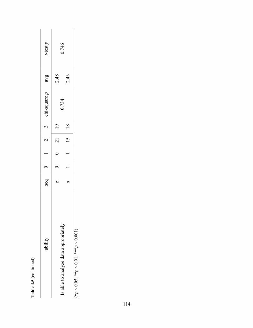
114
Table 4.5 (continued)
114
Tab
le 4
.5 (c
ontin
ued)
abili
ty
seq
0 1
2 3
chi-s
quar
e p
avg
t-tes
t p
e 0
0 21
19
2.
48
Is a
ble
to a
naly
ze d
ata
appr
opria
tely
s
1 1
15
18
0.73
4 2.
43
0.74
6
(*p
< 0.
05, *
*p <
0.0
1, *
**p
< 0.
001)

115
We see that only the ability to minimize uncertainty differs statistically significantly between the
two groups. All of the other abilities are indistinguishable between the two groups.
In Table 4.5, the three laboratory sessions under consideration are combined together so that
we can investigate individual scientific reasoning abilities. Without combining them, the
numbers in each category are insufficient for statistical analysis. Alternatively, we can combine
ratings of scientific abilities into a cumulative score and compare exploratory and scaffolded
sequences across different laboratory sessions. These results are displayed in Table 4.6.
Table 4.6: Comparison of exploratory and scaffolded sequences by laboratory.
variable Exploratory N SE Scaffolded N SE t-test p value
Lab 3 34.77 13 1.20 31.45 11 1.15 0.060
Lab 4 33.07 14 1.01 28.77 13 1.32 0.017*
Lab 5 27.69 13 1.10 28.64 11 1.12 0.554
Total 31.88 40 0.78 29.57 35 0.72 0.035* (*p < 0.05, **p < 0.01, ***p < 0.001)
Students’ cumulative exhibition of scientific reasoning abilities in the exploratory sequence is
marginally significantly better in the third session and significantly better in the fourth session.
When students from both sequences engage with the exploratory activities in the fifth session,
the difference vanishes.
4.4.2 Scientific Reasoning Abilities over Time
The assessment methods employed here are well suited for investigation of the acquisition of
scientific reasoning skills, regardless of which sequence of activities in which students engaged.

116
We focus on five of the scientific reasoning abilities discussed above to better understand how
student exhibition of these abilities changes over the duration of the semester. The five abilities
are: (1) the ability to devise an explanation for an observed pattern, (2) the ability to identify the
assumptions, (3) the ability to determine specifically the way in which assumptions might affect
the prediction/results, (4) the ability to identify sources of experimental uncertainty and (5) the
ability to evaluate specifically how identified experimental uncertainties may affect the data. We
select these five abilities not only because they afford us insights into student engagement, but
also because they afford us the capacity to compare these students’ exhibition of these abilities –
or lack thereof – to that of students from other institutions where analogous studies have been
conducted (Deardorff, 2001; Etkina et al., 2006, 2010, 2008; Lippmann, 2003). Data are
presented here; comparisons are discussed in the subsequent section.
Figure 4.2 is the first of five figures designed to display the exhibition of scientific reasoning
abilities over the duration of the semester. Each color represents a different rating, and the width
of each color represents the fraction of the number of labs submitted that received that rating.
The five bi-weekly labs are represented along the descending vertical axis. Even though
differences between the exploratory and scaffolded sequences are not the primary focus here, the
groups are visually represented by striped and solid bars, respectively, for the third, fourth and
fifth laboratory sessions.
Figure 4.2 displays students’ ability to devise an explanation for an observed pattern.
Students do not exhibit this ability very strongly in their reports from the first session; however,
this is in keeping with other abilities, as students generally responded to discussion questions
with very short answers and limited explanations. We cannot determine whether this resulted
from the step-by-step instructional format of the activities or the mismatch between students’

117
expectations and the novel approach to assessment. In the second session, students demonstrated
the ability much more clearly. In the third session, which was the first time that the ability was
not explicitly stated as part of the assessment criteria for the reports, students’ exhibition of the
activity declined. The pattern repeats through the fourth and fifth sessions, when the ability once
again reappears and then disappears as part of the explicit assessment criteria. This suggests that
students’ demonstration of this ability, although strong, is not sustained when the ability is not
emphasized.
Figure 4.2: Students’ ability to devise an explanation for an observed pattern (Nreport = 131). Each color represents a different rubric score, and the width of each color represents the fraction of the number of labs submitted that received that rubric score. Striped bars represent exploratory sequence labs and solid bars represent scaffolded sequence labs.

118
The ability to identify assumptions that are made when making observations, testing a
hypothesis or solving a problem in the laboratory is one of several important abilities that
students struggle to exhibit consistently (Etkina et al., 2010, 2008). As shown in Figure 4.3,
students do not exhibit the ability in reports from the first session, improve substantially in
reports from the second session, but then appear to plateau – or perhaps even regress – in reports
from subsequent sessions. Students tend to list several general assumptions rather than
considering factors that actually could affect the experiment if they are not as assumed.
Figure 4.3: Students’ ability to identify assumptions (Nreport = 131). Each color represents a different
rubric score, and the width of each color represents the fraction of the number of labs submitted that received that rubric score. Striped bars represent exploratory sequence labs and solid bars represent scaffolded sequence labs.

119
Even more complex than the ability to identify assumptions is the ability to determine the
effects of assumptions; students exhibit this ability when they go beyond merely stating the
necessary assumptions and actually describe how such factors, were they not as assumed, would
affect the experiment. Figure 4.4 highlights the fact that students struggle with this ability
throughout the course. They steadily improve in their ability to identify the effects (which is
rated at “2”), but struggle immensely with taking the next step and validating the assumptions.
Figure 4.4: Students’ ability to determine specifically the way in which assumptions might affect the prediction/results (Nreport = 131). Each color represents a different rubric score, and the width of each color represents the fraction of the number of labs submitted that received that rubric score. Striped bars represent exploratory sequence labs and solid bars represent scaffolded sequence labs.
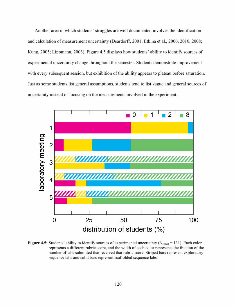
120
Another area in which students’ struggles are well documented involves the identification
and calculation of measurement uncertainty (Deardorff, 2001; Etkina et al., 2006, 2010, 2008;
Kung, 2005; Lippmann, 2003). Figure 4.5 displays how students’ ability to identify sources of
experimental uncertainty change throughout the semester. Students demonstrate improvement
with every subsequent session, but exhibition of the ability appears to plateau before saturation.
Just as some students list general assumptions, students tend to list vague and general sources of
uncertainty instead of focusing on the measurements involved in the experiment.
Figure 4.5: Students’ ability to identify sources of experimental uncertainty (Nreport = 131). Each color represents a different rubric score, and the width of each color represents the fraction of the number of labs submitted that received that rubric score. Striped bars represent exploratory sequence labs and solid bars represent scaffolded sequence labs.

121
Also, students struggle with distinguishing between assumptions – elements of the environment
or apparatus that can be considered negligible, constant or predictable – and sources of
uncertainty – measurements of attributes or quantities that have some finite accuracy and
precision. Often students confuse the two concepts or simply pool them together. The ability to
distinguish between assumptions and uncertainties, however, is not formally assessed.
Figure 4.6: Students’ ability to evaluate specifically how identified experimental uncertainties may affect the data (Nreport = 104). Each color represents a different rubric score, and the width of each color represents the fraction of the number of labs submitted that received that rubric score. Striped bars represent exploratory sequence labs and solid bars represent scaffolded sequence labs. This ability was not required in activities from the fourth session, so no data are recorded.
Finally, we highlight students’ ability to evaluate specifically how identified experimental
uncertainties may affect the data in Figure 4.6. This is more difficult than merely identifying
122
uncertainties, as demonstrated by the low ratings through the reports from the first three sessions.
Reports from the fourth session are not included here because the experiments were almost
entirely qualitative in nature; students made observations and collected data, but the sources of
uncertainty were not quantifiable. Students showed much stronger abilities in reports from the
fifth session, though their use of linear regression techniques in this particular activity made
evaluation of error somewhat different – and, perhaps, more straightforward – than in prior
activities.
Students improve throughout the semester in many of the abilities that we assess.
Nonetheless, at the end of the semester, they do not saturate some of these abilities involving
uncertainty and assumption that are very closely tied to the goals of the instructional laboratory.
4.5 Discussion
Just as the results presented above branch in two main directions, we discuss each one of these
branches below. We then connect our findings to the theoretical elements of transfer, address the
limitations of this work and suggest potential future directions.
4.5.1 Comparison of Exploratory and Scaffolded Sequences
The comparative analysis of students from two sequences of laboratory activities, one that is
more exploratory and another that is more explicitly scaffolded, indicates that there are
differences between the two groups, although the differences are slight. Students engaged in the
exploratory, SCL-like sequence exhibit better scientific reasoning and data handling abilities.
Among surveys and course performance metrics, only the post-course DHD reveals a
statistically significant difference between the groups. No single item on the 23-question survey
123
is associated with this difference. However, the difference between the two groups in actual units
is only 1.7 questions. Perhaps it is not surprising that both groups performed relatively poorly, as
the laboratory activities were not explicitly designed to improve performance on the DHD. Many
of the questions on the survey require students to utilize specific knowledge and strategies,
whereas the laboratory activities attempt to engender and promote scientific ways of thinking. In
other words, the DHD is focused on a dimension of learning that seems to be orthogonal to the
dimensions that are central to the design of the laboratory sequences. So, while this relationship
may be suggestive of potentially larger differences in an untapped dimension of student learning,
the slight difference is not especially meaningful by itself.
Unlike the DHD, the scientific reasoning abilities are precisely aligned with the learning
goals in the laboratory. We once again measure almost no differences between the two sequences
across many of the abilities assessed. However, the strongly statistically significant difference
between students from each sequence in their ability to minimize uncertainty may reveal
information about the roots of the persistent slight differences. The freedom afforded to students
in the exploratory sequence may allow them to design and conduct experiments with which they
feel the most comfortable engaging. The heuristically scaffolded activities require students to
occasionally address questions that challenge their expectations about what a solution might look
like. Minimizing uncertainty, for instance, is easier to think about when an experiment results in
a quantitative value that can be averaged over multiple trials. If the experiment is qualitative,
considering and minimizing uncertainty are not necessarily so familiar to students.
Overall, less scaffolding is associated with slightly improved exhibition of scientific
reasoning abilities. This may result from students engaging more critically throughout the
activities, or it may result from students choosing the path about which they are more

124
comfortable and confident. The latter cause doesn’t necessarily mean that the exploratory
approach is weaker; as we discussed extensively in Chapter Three, confidence and self-efficacy
are strongly associated with positive learning outcomes. Perhaps the fact that the reports from the
two sequences are indistinguishable in the fifth laboratory meeting suggests that the slight
differences are superficial (though we must be careful not to draw conclusions from a single
laboratory activity).
Practically speaking, as the differences in all facets of assessment are quite small, there is no
evidence to suggest that either sequence is better or worse than the other according to the metrics
assessed here. Others report that both of these approaches promote stronger exhibition of
scientific reasoning skills and time spent sense-making than traditional laboratories (Etkina et al.,
2010; Lippmann, 2003); therefore, our findings suggest that both approaches are viable
alternatives for laboratory instruction.
4.5.2 Scientific Reasoning Abilities over Time
Some skills, such as the ability to evaluate the consistency of different representations, the ability
to design a reliable experiment and the ability to make a reasonable prediction based on a
hypothesis, seem to saturate early in the semester and remain saturated throughout. Other skills,
such as those displayed in Figure 4.2, Figure 4.3 and Figure 4.5, either plateau or decline
throughout the semester. Still others, such as those displayed in Figure 4.4 and Figure 4.6,
increase throughout the semester but do not saturate.
These observations suggest that, regarding many of the scientific reasoning abilities of
interest, five bi-weekly laboratory sessions are not sufficient for acquisition. Etkina and
colleagues report that only after eight weekly sessions in which students conduct heuristically
125
scaffolded design laboratories do they begin to achieve mastery of scientific abilities (Etkina et
al., 2008). We cannot determine whether the amount of time, number of meetings, frequency of
meetings, or the combination of these factors accounts for their observation. Nonetheless, our
findings suggest that fewer meetings at a lower frequency, in spite of differences in student
population, are not as effective as activities conducted elsewhere. More opportunities for
students to engage in laboratory activities allow for (1) longer duration of scaffolding, (2) more
varied scaffolding and (3) more distributed scaffolding; in spite of the fact that only a fraction of
the scientific reasoning abilities were incorporated for assessment, students were clearly
overwhelmed by the information.
4.5.3 Transfer
As mentioned before, in linking transfer to teaching practices, Georghiades highlights
metacognition, and specifically metacognitive activities together with social activities, as a way
of overcoming the decay in conceptual change (Georghiades, 2000). This notion applies to both
the exploratory, SCL-like sequence of laboratory activities and the heuristically scaffolded, ISLE
design-like sequence, and it may also suggest an alternative explanation for why the differences
between the two sequences are so slight. The heuristic scaffolding, while not explicitly
metacognitive, provides a template for the kinds of questions students can ask themselves later,
in a less scaffolded environment; in other words, the scaffolding is a template for metacognition.
The exploratory activities, although not explicitly scaffolded, promote extensive interaction
among students. So it is perhaps a misnomer to suggest that only one sequence is scaffolded;
both are scaffolded in such ways as to emphasize different aspects of learning.
126
Explicitly regarding transfer, Lobato discusses three key mechanisms: (1) “focusing
phenomena,” features in a classroom environment that direct students’ attention toward certain
properties or patterns, (2) “social framing,” a way of framing both activities and students’ roles
as being connected with other contexts in which the learning experiences are relevant, and (3)
“discernment of differences,” in which students consider differences between situations to
ultimately refine transfer ability (Lobato, 2006). In these laboratory sessions, the focusing
phenomena are the activities; the printed materials are designed to consistently focus students on
the relevant goals and scientific abilities from session to session, even as the content-related
aspects of the activities change. Social framing occurs as students return to the same room,
sometimes reforming the same group, to engage in these activities; the expectations for the
various interactions that take place – among students as they discuss the activities, between
instructors and students, and even among the whole class – are consistent from session to
session, and therefore reinforce the reasoning skills that are associated with those interactions.
Although the discernment of differences is not explicitly reinforced, the different ways in which
scientific reasoning skills are applied from one activity to the next require students to consider
such differences. Thus, all three of these features play an important role in the activities studied
here.
4.5.4 Limitations
Although we were able to access many dimensions of student learning and engagement in the
introductory physics laboratory, we note some specific limitations.
With only five bi-weekly meetings, we cannot conclusively establish whether differences –
or the lack thereof – between groups or from one session to the next result from underlying

127
trends or unrelated fluctuations. For example, perhaps the difference in exhibited abilities
between students from the two sequences in the fifth session disappears because the groups are
not actually different, or perhaps it disappears because those specific activities happen to mask
the actual differences. Even if there were ten labs, however, I doubt we would have chosen to
implement multiple overlapping activities. One way to overcome this limitation is to continue
conducting studies like this in different courses and different institutions until the amount of data
suppresses the noise enough for underlying trends to emerge. Alternatively, we can conduct
more extensive qualitative analysis of students’ reasoning to better understand how the
intricacies of each specific laboratory session might affect our conclusions. This may be the
more fruitful of the two alternatives, as the system is very complicated and not thoroughly
understood.
Although we could not implement video recordings for discourse analysis as a component of
this study, such data could certainly inform the question of whether students in the exploratory
sequence exhibit stronger reasoning abilities because they are more inclined to make choices
about which they are confident or because they are more critically engaged. This remains an
open question for future investigation.
4.6 Conclusion
Ultimately, we find that students who engage in two different sequences of laboratory activities –
exploratory and heuristically scaffolded – both demonstrate similarly enhanced scientific
reasoning skills; the students who participate in the former sequence slightly outperform those in
the latter, though perhaps the difference in performance only occur while the groups are
engaging in different activities, as it disappears when the two groups engage in identical final

128
laboratory activities. Regardless of group, some important skills are either not exhibited or
retained by many of the students, suggesting that five bi-weekly meetings are not sufficient for
acquisition and demonstration of these abilities.

129
Chapter Five
Conclusions
At the end of Chapter One, we suggest that the best forms of assessment collect as much
information as possible about student learning outcomes, but the interpretation of that
information is essential. Each of the projects described in this work represent our efforts to
exemplify this statement through physics education research.
Here we review the conclusions drawn from the three preceding chapters and elaborate on
the common theme of assessment from the instructor’s perspective.

130
5.1 Review
In Chapter Two, we describe the challenges that instructors may encounter when attempting to
interpret results after implementing the Force Concept Inventory (FCI). To solve these
challenges, we introduce stratagrams: simple visualizations of student performance that
highlight the rate of students becoming Newtonian thinkers, and therefore provide a clear,
informative basis for both assessing a single class and comparing performance between a small
number of classes. Whereas normalized gain, the standard metric of success on the FCI, is
certainly useful when many different classes are involved, data show that several factors,
particularly losses and differences in pre-test performance, complicate the interpretation of
normalized gain when it is used to compare FCI performance between small numbers of classes.
In such comparisons, fluctuations among different calculations of normalized gain are not
negligible and can significantly affect the outcome. Moreover, none of the variations of
normalized gain address the fact that users of normalized gain cannot say which students in the
class are improving, and none of them highlight differences in student population. Thus,
stratagrams fill an instructive, accessible and previously unexplored niche in the array of tools
that are available to instructors for learning the most from student performance on the FCI, as
well as other similar pre-test and post-test conceptual inventories.
In Chapter Three, we find that students’ expressions of confusion transect many different
dimensions of performance, attitude and identity. Students who express more confusion tend to
also express lower confidence, lower self-efficacy, and, to a slight degree, weaker performance
on reading exercises. However, when we control for all of these factors, students who express
confusion tend to also perform better overall, as measured by final grade. Thus, we suggest that,

131
when relevant factors are not controlled for, expressions of confusion may be either bad or
merely uninformative; but when relevant factors are controlled for, assuming that we are
interested in relating assessment of confusion to final grades, confusion is good. In other words,
we are able to identify and isolate the productive role of confusion using surveys and reading
assignment activities that are entirely accessible to instructors. Thus, if instructors assess
confusion as presented here, then they can monitor the productive role of confusion, assess
students’ metacognition as they engage in activities, and perhaps even find ways to promote such
constructive expressions of confusion.
Finally, in Chapter Four, we explore students’ exhibition of scientific reasoning abilities in
the introductory physics laboratory. We find that students who engage in two different sequences
of laboratory activities – exploratory and heuristically scaffolded – both demonstrate similarly
enhanced scientific reasoning skills; the students who participate in the former sequence slightly
outperform those in the latter, though perhaps the difference in performance only occur while the
groups are engaging in different activities, as it disappears when the two groups engage in
identical final laboratory activities. Practically speaking, as the differences in all facets of
assessment are quite small, there is no evidence to suggest that either sequence is better or worse
than the other according to the metrics assessed here. Others report that both of these approaches
promote stronger exhibition of scientific reasoning skills and time spent sense-making than
traditional laboratories (Etkina et al., 2010; Lippmann, 2003); therefore, our findings suggest that
both approaches are viable alternatives for laboratory instruction. Regardless of group, though,
some important skills are either not exhibited or retained by many of the students, which
suggests that five bi-weekly meetings are not sufficient for acquisition and demonstration of the
most important abilities. More opportunities for students to engage in laboratory activities allow
132
for (1) longer duration of scaffolding, (2) more varied scaffolding and (3) more distributed
scaffolding.
In spite of the differences in scope, context and analytical techniques, these three projects are
all driven by the motivation to better design, understand and implement assessment to improve
students’ learning and engagement in physics. Stratagrams incorporate the intended goals of the
FCI into a precise means of assessing the performance of a class. We better understand confusion
as a means of assessing both positive and negative ways in which students think and feel about
physics, and how that relates to success in physics. Using carefully designed rubrics for
assessment of scientific reasoning, we can make clear statements about pedagogical approaches
to laboratory instruction and implement changes based on those assessments.
In short, we present insights into three unique and important avenues of assessment in the
physics classroom and laboratory through extensive data collection and close inspection of the
underlying relationships.
5.2 The Goal of Assessment
Even though the focus of this work is assessment, the first step in the instructional process
should always be the determination of goals (Wiggins, 2005). One cannot assess FCI
performance without first establishing our goal in administering the survey. One cannot assess
the role of students’ expressions of confusion, or the value of that role, without first determining
which outcomes are considered positive, negative or neutral. We cannot assess the effectiveness
of alternate approaches to laboratory instruction without first establishing the goals of laboratory
instruction. Once the goals are established, assessment is simply a matter of determining the
proper questions to pose and interpreting what different answers could mean.

133
Building from goal to assessment, and then towards instruction, captures the essence of
Understanding by Design (Wiggins, 2005). Regarding assessment, they write:
We are obligated to consider the assessment evidence implied by the outcomes sought, rather than thinking about assessment primarily as a means for generating grades. Given the goals, what performance evidence signifies that they have been met? Given the essential questions, what evidence would show that the learner had deeply considered them? Given the understandings, what would show that the learner “got it”? We urge teachers to consider a judicial analogy as they plan assessment. Think of students as juries think of the accused: innocent (of understanding, skill, and so on) until proven guilty by a preponderance of evidence that is more than circumstantial. (p. 148)
We hope that the work presented here, in addition to abiding by the criteria described, sheds
some light on the ways in which instructors can use such tools in physics classrooms and
instructional laboratories.

134
References
Adams, W. K., Perkins, K. K., Podolefsky, N. S., Dubson, M., Finkelstein, N. D., & Wieman, C. E. (2006). New instrument for measuring student beliefs about physics and learning physics: The Colorado Learning Attitudes about Science Survey. Physical Review Special Topics - Physics Education Research, 2(1), 010101. doi:10.1103/PhysRevSTPER.2.010101
Adams, Wendy K, Paulson, A., & Wieman, C. E. (2008). What Levels of Guidance Promote Engaged Exploration with Interactive Simulations? AIP Conference Proceedings, 1064(1), 59–62. doi:doi:10.1063/1.3021273
Andrew, S. (1998). Self-efficacy as a predictor of academic performance in science. Journal of Advanced Nursing, 27(3), 596–603. doi:10.1046/j.1365-2648.1998.00550.x
Antti Savinainen and Philip Scott. (2002). The Force Concept Inventory: a tool for monitoring student learning. Physics Education, 37(1), 45.
Bandura, A. (1977). Self-efficacy: Toward a unifying theory of behavioral change. Psychological Review, 84(2), 191–215. doi:10.1037/0033-295X.84.2.191
Bandura, A. (1986). The Explanatory and Predictive Scope of Self-Efficacy Theory. Journal of Social and Clinical Psychology, 4(3), 359–373. doi:10.1521/jscp.1986.4.3.359
Bandura, A. (1989). Human agency in social cognitive theory. American Psychologist, 44(9), 1175–1184. doi:10.1037/0003-066X.44.9.1175
Bao, L. (2006). Theoretical comparisons of average normalized gain calculations. American Journal of Physics, 74(10), 917. doi:10.1119/1.2213632
Bao, L., & Redish, E. F. (2006). Model analysis: Representing and assessing the dynamics of student learning. Physical Review Special Topics - Physics Education Research, 2(1), 010103.
Barnett, S. M., & Ceci, S. J. (2002). When and where do we apply what we learn?: A taxonomy for far transfer. Psychological Bulletin, 128(4), 612–637. doi:10.1037/0033-2909.128.4.612
Barrow, L. (2006). A Brief History of Inquiry: From Dewey to Standards. Journal of Science Teacher Education, 17(3), 265–278. doi:10.1007/s10972-006-9008-5
Bransford, J. D., Brown, A. L., & Cocking, R. R. (Eds.). (2000). How people learn: Brain, mind, experience, and school: Expanded Edition. Washington, DC: National Academy Press.
Carraher, D., & Schliemann, A. (2002). The Transfer Dilemma. Journal of the Learning Sciences, 11(1), 1–24. doi:10.1207/S15327809JLS1101_1

135
Cheng, K. K., Thacker, B. A., Cardenas, R. L., & Crouch, C. (2004). Using an online homework system enhances students’ learning of physics concepts in an introductory physics course. American Journal of Physics, 72(11), 1447. doi:10.1119/1.1768555
Cobb, P., & Bowers, J. (1999). Cognitive and Situated Learning Perspectives in Theory and Practice. Educational Researcher, 28(2), 4–15. doi:10.3102/0013189X028002004
Coletta, V. P., & Phillips, J. A. (2005). Interpreting FCI scores: Normalized gain, preinstruction scores, and scientific reasoning ability. American Journal of Physics, 73(12), 1172–1182. doi:10.1119/1.2117109
Confrey, J. (1990). Chapter 8: What Constructivism Implies for Teaching. Journal for Research in Mathematics Education. Monograph, 4, 107–210. doi:10.2307/749916
Costello, A., & Osborne, J. (2005). Best practices in exploratory factor analysis: four recommendations for getting the most from your analysis. Practical Assessment Research & Evaluation, 10(7). Retrieved from http://pareonline.net/getvn.asp?v=10&n=7
Crouch, C. (2000, January 18). Confusion: Students’ Perception vs. Reality. Contributed presented at the American Association of Physics Teachers Winter Meeting, 2000, Kissimmee, FL.
Crouch, C. H., & Mazur, E. (2001). Peer Instruction: Ten years of experience and results. American Journal of Physics, 69(9), 970. doi:10.1119/1.1374249
Cummings, K., Marx, J., Thornton, R., & Kuhl, D. (1999). Evaluating innovation in studio physics. American Journal of Physics, 67(S1), S38–S44. doi:10.1119/1.19078
Dancy, M. H. (2000). Investigating animations for assessment with an animated version of the Force Concept Inventory (Ph.D.). North Carolina State University, Raleigh, NC.
Deardorff, D. L. (2001). Introductory physics students’ treatment of measurement uncertainty. North Carolina State University, Raleigh, NC. Retrieved from http://adsabs.harvard.edu/abs/2001PhDT.......132D
Dellwo, D. R. (2010). Course assessment using multi-stage pre/post testing and the components of normalized change. Journal of the Scholarship of Teaching and Learning, 10(1), 55–67.
diSessa, A. A. (2006). A History of Conceptual Change Research: Threads and Fault Lines. The Cambridge handbook of: The learning sciences. (pp. 265–281). New York, NY, US: Cambridge University Press.
Domelen, D. J. V., & Heuvelen, A. V. (2002). The effects of a concept-construction lab course on FCI performance. American Journal of Physics, 70(7), 779–780. doi:10.1119/1.1377284

136
Dunning, D., Griffin, D. W., Milojkovic, J. D., & Ross, L. (1990). The overconfidence effect in social prediction. Journal of Personality and Social Psychology, 58(4), 568–581.
Engelbrecht, J., Harding, A., & Potgieter, M. (2005). Undergraduate students’ performance and confidence in procedural and conceptual mathematics. International Journal of Mathematical Education in Science and Technology, 36(7), 701–712. doi:10.1080/00207390500271107
Etkina, E., Karelina, A., & Ruibal-Villasenor, M. (2008). How long does it take? A study of student acquisition of scientific abilities. Physical Review Special Topics - Physics Education Research, 4(2), 020108. doi:10.1103/PhysRevSTPER.4.020108
Etkina, E., Karelina, A., Ruibal-Villasenor, M., Rosengrant, D., Jordan, R., & Hmelo-Silver, C. E. (2010). Design and Reflection Help Students Develop Scientific Abilities: Learning in Introductory Physics Laboratories. Journal of the Learning Sciences, 19(1), 54–98. doi:10.1080/10508400903452876
Etkina, E., Van Heuvelen, A., White-Brahmia, S., Brookes, D. T., Gentile, M., Murthy, S., Rosengrant, D., et al. (2006). Scientific abilities and their assessment. Physical Review Special Topics - Physics Education Research, 2(2), 020103. doi:10.1103/PhysRevSTPER.2.020103
Everson, H. T., & Tobias, S. (1998). The ability to estimate knowledge and performance in college: A metacognitive analysis. Instructional Science, 26(1), 65–79. doi:10.1023/A:1003040130125
Fencl, H. S., & Scheel, K. R. (2004). Pedagogical approaches, contextual variables, and the development of student self‐efficacy in undergraduate physics courses. AIP Conference Proceedings, 720(1), 173–176. doi:doi:10.1063/1.1807282
Finkelstein, N. D., & Pollock, S. J. (2005). Replicating and understanding successful innovations: Implementing tutorials in introductory physics. Physical Review Special Topics - Physics Education Research, 1(1), 010101.
Flavell, J. H. (1979). Metacognition and cognitive monitoring: A new area of cognitive–developmental inquiry. American Psychologist, 34(10), 906–911. doi:10.1037/0003-066X.34.10.906
Galloway, R. K., Bates, S. P., Maynard-Casely, H. E., & Slaughter, K. A. (in press). Data Handling Diagnostic: Design, Validation and Preliminary Findings. Physical Review Special Topics: Physics Education Research.
Garofalo, J., & Lester, F. K. (1985). Metacognition, Cognitive Monitoring, and Mathematical Performance. Journal for Research in Mathematics Education, 16(3), 163. doi:10.2307/748391

137
Georghiades, P. (2000). Beyond conceptual change learning in science education: focusing on transfer, durability and metacognition. Educational Research, 42(2), 119–139. doi:10.1080/001318800363773
Gigerenzer, G., Hoffrage, U., & Kleinbölting, H. (1991). Probabilistic mental models: A Brunswikian theory of confidence. Psychological Review, 98(4), 506–528. doi:10.1037/0033-295X.98.4.506
Greeno, J. G. (1997). On Claims That Answer the Wrong Questions. Educational Researcher, 26(1), 5–17. doi:10.3102/0013189X026001005
Gunstone, R. F., & White, R. T. (1981). Understanding of gravity. Science Education, 65(3), 291–299. doi:10.1002/sce.3730650308
Hake, R. R. (1998). Interactive-engagement versus traditional methods: A six-thousand-student survey of mechanics test data for introductory physics courses. American Journal of Physics, 66, 64–74.
Hake, R. R. (2002, August). Relationship of Individual Student Normalized Learning Gains in Mechanics with Gender, High-School Physics, and Pretest Scores on Mathematics and Spatial Visualization. submitted to the Physics Education Research Conference, Boise, Idaho.
Hake, R. R, Wakeland, R., Bhattacharyya, A., & Sirochman, R. (1994). Assessment of individual student performance in an introductory mechanics course. AAPT Announcer, 24(4), 76.
Hake, Richard R. (1992). Socratic pedagogy in the introductory physics laboratory. The Physics Teacher, 30(9), 546–552. doi:10.1119/1.2343637
Halloun, I. A., & Hestenes, D. (1985). The initial knowledge state of college physics students. American Journal of Physics, 53(11), 1043–1055. doi:10.1119/1.14030
Halloun, I., & Hestenes, D. (1996). The search for conceptual coherence in FCI data. preprint.
Hammer, D. (1994). Epistemological Beliefs in Introductory Physics. Cognition and Instruction, 12(2), 151–183. doi:10.1207/s1532690xci1202_4
Hammer, D. (1996). More than misconceptions: Multiple perspectives on student knowledge and reasoning, and an appropriate role for education research. American Journal of Physics, 64(10), 1316–1325. doi:10.1119/1.18376
Hammer, D., & Elby, A. (2003). Tapping Epistemological Resources for Learning Physics. Journal of the Learning Sciences, 12(1), 53–90. doi:10.1207/S15327809JLS1201_3
Hart, J. T. (1965). Memory and the feeling-of-knowing experience. Journal of Educational Psychology, 56(4), 208–216. doi:10.1037/h0022263

138
Heller, P. (1995). Interpreting the force concept inventory: A reply to Hestenes and Halloun. The Physics Teacher, 33(8), 503. doi:10.1119/1.2344279
Heller, Patricia, & Hollabaugh, M. (1992). Teaching problem solving through cooperative grouping. Part 2: Designing problems and structuring groups. American Journal of Physics, 60(7), 637–644. doi:10.1119/1.17118
Heller, Patricia, Keith, R., & Anderson, S. (1992). Teaching problem solving through cooperative grouping. Part 1: Group versus individual problem solving. American Journal of Physics, 60, 627–636.
Hestenes, D., & Halloun, I. (1995). Interpreting the Force Concept Inventory: A Response to March 1995 Critique by Huffman and Heller. The Physics Teacher, 33, 502–506.
Hestenes, D., Wells, M., & Swackhamer, G. (1992). Force Concept Inventory. The Physics Teacher, 30, 141–158.
Hofstein, A., & Lunetta, V. N. (1982). The Role of the Laboratory in Science Teaching: Neglected Aspects of Research. Review of Educational Research, 52(2), 201–217.
Holton, D., & Clarke, D. (2006). Scaffolding and metacognition. International Journal of Mathematical Education in Science and Technology, 37(2), 127–143. doi:10.1080/00207390500285818
Huffman, D., & Heller, P. (1995). What does the force concept inventory actually measure? The Physics Teacher, 33(3), 138–143. doi:10.1119/1.2344171
Karelina, A. (2011, November 29). personal correspondence.
Karelina, A., & Etkina, E. (2007). Acting like a physicist: Student approach study to experimental design. Physical Review Special Topics - Physics Education Research, 3(2), 020106. doi:10.1103/PhysRevSTPER.3.020106
Kirschner, P. A., Sweller, J., & Clark, R. E. (2006). Why Minimal Guidance During Instruction Does Not Work: An Analysis of the Failure of Constructivist, Discovery, Problem-Based, Experiential, and Inquiry-Based Teaching. Educational Psychologist, 41(2), 75–86. doi:10.1207/s15326985ep4102_1
Knight, J. K., & Wood, W. B. (2005). Teaching more by lecturing less. Life Sciences Education, 4(4), 298.
Koch, A. (2001). Training in metacognition and comprehension of physics texts. Science Education, 85(6), 758–768. doi:10.1002/sce.1037
Kost, L. E., Pollock, S. J., & Finkelstein, N. D. (2009). Unpacking Gender Differences in Students’ Perceived Experiences in Introductory Physics. Proceedings of the 2009 Physics Education Research Conference.

139
Kruger, J., & Dunning, D. (1999). Unskilled and unaware of it: How difficulties in recognizing one’s own incompetence lead to inflated self-assessments. Journal of Personality and Social Psychology, 77(6), 1121–1134.
Kung, R. L. (2005). Teaching the concepts of measurement: An example of a concept-based laboratory course. American Journal of Physics, 73(8), 771–777. doi:10.1119/1.1881253
L. Deslauriers, E. Schelew, and C. Wieman. (2011). Improved Learning in a Large-Enrollment Physics Class. Science, 332(6031), 862–864.
Lasry, N. (2008). Clickers or flashcards: Is there really a difference? The Physics Teacher, 46, 242.
Lasry, Nathaniel, Mazur, E., & Watkins, J. (2008). Peer instruction: From Harvard to the two-year college. American Journal of Physics, 76(11), 1066. doi:10.1119/1.2978182
Lave, J. (1988). Cognition in Practice: Mind, Mathematics and Culture in Everyday Life. Cambridge University Press.
Lent, R. W., Brown, S. D., & Larkin, K. C. (1984). Relation of self-efficacy expectations to academic achievement and persistence. Journal of Counseling Psychology, 31(3), 356–362. doi:10.1037/0022-0167.31.3.356
Lent, R. W., Brown, S. D., & Larkin, K. C. (1987). Comparison of three theoretically derived variables in predicting career and academic behavior: Self-efficacy, interest congruence, and consequence thinking. Journal of Counseling Psychology, 34(3), 293–298. doi:10.1037/0022-0167.34.3.293
Lerman, S. (1996). Intersubjectivity in Mathematics Learning: A Challenge to the Radical Constructivist Paradigm? Journal for Research in Mathematics Education, 27(2), 133–150. doi:10.2307/749597
Li, S. L., & Demaree, D. (2012). Assessing physics learning identity: Survey development and validation. AIP Conference Proceedings, 1413(1), 247–250. doi:doi:10.1063/1.3680041
Linnenbrink, E. A., & Pintrich, P. R. (2003). THE ROLE OF SELF-EFFICACY BELIEFS INSTUDENT ENGAGEMENT AND LEARNING INTHECLASSROOM. Reading & Writing Quarterly, 19(2), 119–137. doi:10.1080/10573560308223
Lippmann Kung, R., & Linder, C. (2007). Metacognitive activity in the physics student laboratory: is increased metacognition necessarily better? Metacognition and Learning, 2(1), 41–56. doi:10.1007/s11409-007-9006-9
Lippmann, R. F. (2003). Students’ understanding of measurement and uncertainty in the physics laboratory: Social construction, underlying concepts, and quantitative analysis. University of Maryland, College Park, MD, United States.
140
Lobato, J. (2003). How Design Experiments Can Inform a Rethinking of Transfer andViceVersa. Educational Researcher, 32(1), 17–20. doi:10.3102/0013189X032001017
Lobato, J. (2006). Alternative Perspectives on the Transfer of Learning: History, Issues, and Challenges for Future Research. Journal of the Learning Sciences, 15(4), 431–449. doi:10.1207/s15327809jls1504_1
Lorenzo, M., Crouch, C. H., & Mazur, E. (2006). Reducing the gender gap in the physics classroom. American Journal of Physics, 74(2), 118. doi:10.1119/1.2162549
MacIsaac, D., & Falconer, K. (2002). Reforming Physics Instruction Via RTOP. The Physics Teacher, 40(8), 479–485.
Mahajan, S. (2005, December 16). Observations on teaching first-year physics. Retrieved from http://arxiv.org/PS_cache/physics/pdf/0512/0512158v1.pdf
Maloney, D. P., O’Kuma, T. L., Hieggelke, C. J., & Van Heuvelen, A. (2001). Surveying students’ conceptual knowledge of electricity and magnetism. American Journal of Physics, 69(S1), S12. doi:10.1119/1.1371296
Marx, J. D., & Cummings, K. (2007). Normalized change. American Journal of Physics, 75(1), 87–91. doi:10.1119/1.2372468
Mazur, E. (1997). Peer instruction: A user’s manual. Upper Saddle River, New Jersey: Prentice Hall.
McDermott, L. C., & Shaffer, P. S. (1992). Research as a guide for curriculum development: An example from introductory electricity. Part I: Investigation of student understanding. American Journal of Physics, 60(11), 994–1003. doi:10.1119/1.17003
McDermott, L. C., & Shaffer, P. S. (2001). Tutorials in Introductory Physics. Prentice Hall College Div.
McKagan, S. B., Perkins, K. K., & Wieman, C. E. (2007). Reforming a large lecture modern physics course for engineering majors using a PER-based design. AIP Conference Proceedings, 883, 34–37. doi:Article
McKeachie, W. J. (1987). Cognitive skills and their transfer: Discussion. International Journal of Educational Research, 11(6), 707–712. doi:10.1016/0883-0355(87)90010-3
Meltzer, D. E. (2002). The relationship between mathematics preparation and conceptual learning gains in physics: A possible ``hidden variable’’ in diagnostic pretest scores. American Journal of Physics, 70(12), 1259–1268.
Meltzer, D. E., & Manivannan, K. (2002). Transforming the lecture-hall environment: the fully interactive physics lecture.(Abstract). American Journal of Physics, 70, 639(16).
Merriam-Webster, Inc. (2003). Merriam-Webster’s Collegiate Dictionary. Merriam-Webster.
141
Moore, D. S., McCabe, G. P., Duckworth, W. M., & Alwan, L. C. (2008). The Practice of Business Statistics: Using Data for Decisions (2nd ed.). Palgrave.
Morris, G. A., Branum-Martin, L., Harshman, N., Baker, S. D., Mazur, E., Dutta, S., Mzoughi, T., et al. (2006). Testing the test: Item response curves and test quality. American Journal of Physics, 74(5), 449–453. doi:10.1119/1.2174053
Multon, K. D., Brown, S. D., & Lent, R. W. (1991). Relation of self-efficacy beliefs to academic outcomes: A meta-analytic investigation. Journal of Counseling Psychology, 38(1), 30–38. doi:10.1037/0022-0167.38.1.30
Novak, G. M., Gavrin, A., & Wolfgang, C. (1999). Just-in-Time Teaching: Blending Active Learning with Web Technology (1st ed.). Upper Saddle River, NJ, USA: Prentice Hall PTR.
Perkins, D., & Salomon, G. (1989). Are Cognitive Skills Context-Bound? Educational Researcher, 18(1), 16–25. doi:10.3102/0013189X018001016
Piaget, J. (1985). The Equilibration of Cognitive Structures: The Central Problem of Intellectual Development. Chicago: University of Chicago Press.
Piaget, J., Green, D. R., Ford, M. P., & Flamer, G. B. (1971). The Theory of Stages in Cognitive Development. In Measurement and Piaget (pp. 1–11). New York: McGraw-Hill.
Piaget, Jean. (1977). The development of thought: Equilibration of cognitive structures. (Trans A. Rosin). Oxford, England: Viking.
Piaget, Jean. (1980). Adaptation and intelligence : organic selection and phenocopy. Chicago: University of Chicago Press.
Pietsch, J., Walker, R., & Chapman, E. (2003). The relationship among self-concept, self-efficacy, and performance in mathematics during secondary school. Journal of Educational Psychology, 95(3), 589–603. doi:10.1037/0022-0663.95.3.589
Pollock, S. J., Finkelstein, N. D., & Kost, L. E. (2007). Reducing the gender gap in the physics classroom: How sufficient is interactive engagement? Physical Review Special Topics - Physics Education Research, 3(1), 010107.
Posner, G. J., Strike, K. A., Hewson, P. W., Gertzog, W. A., Posner, G. J., Strike, K. A., Hewson, P. W., et al. (1982). Accommodation of a scientific conception: Toward a theory of conceptual change, Accommodation of a scientific conception: Toward a theory of conceptual change. Science Education, Science Education, 66, 66(2, 2), 211, 211–227, 227. doi:10.1002/sce.3730660207, 10.1002/sce.3730660207
Redish, E. F. (2004). A Theoretical Framework for Physics Education Research: Modeling Student Thinking. arXiv:physics/0411149. Retrieved from http://arxiv.org/abs/physics/0411149

142
Redish, E. F., Saul, J. M., & Steinberg, R. N. (1997). On the effectiveness of active-engagement microcomputer-based laboratories. American Journal of Physics, 65(1), 45–54. doi:10.1119/1.18498
Redish, E. F., Saul, J. M., & Steinberg, R. N. (1998). Student expectations in introductory physics. American Journal of Physics, 66(3), 212–224. doi:10.1119/1.18847
Reif, F., & John, M. S. (1979). Teaching physicists’ thinking skills in the laboratory. American Journal of Physics, 47(11), 950–957. doi:10.1119/1.11618
Reif, F., & Reif, F. (1987). Instructional design, cognition, and technology: Applications to the teaching of scientific concepts, Instructional design, cognition, and technology: Applications to the teaching of scientific concepts. Journal of Research in Science Teaching, Journal of Research in Science Teaching, 24, 24(4, 4), 309, 309–324, 324. doi:10.1002/tea.3660240405, 10.1002/tea.3660240405
Reif, Frederick. (1995). Understanding and Teaching Important Scientific Thought Processes. Journal of Science Education and Technology, 4(4), 261–282.
Resnick, L. B. (Ed.). (1976). The nature of intelligence. Oxford, England: Lawrence Erlbaum.
Rickey, D., & Stacy, A. M. (2000). The Role of Metacognition in Learning Chemistry. J. Chem. Educ., 77(7), 915. doi:10.1021/ed077p915
Sawtelle, V. (2011). A Gender Study Investigating Physics Self-Efficacy. FIU Electronic Theses and Dissertations. Retrieved from http://digitalcommons.fiu.edu/etd/512
Schoenfeld, A. H. (1992). Learning to think mathematically: Problem solving, metacognition, and sense making in mathematics. Handbook of research on mathematics teaching and learning: A project of the National Council of Teachers of Mathematics. (pp. 334–370). New York, NY, England: Macmillan Publishing Co, Inc.
Schraw, G., Crippen, K., & Hartley, K. (2006). Promoting Self-Regulation in Science Education: Metacognition as Part of a Broader Perspective on Learning. Research in Science Education, 36(1), 111–139. doi:10.1007/s11165-005-3917-8
Schwab, Joseph J. (1960). Inquiry, the Science Teacher, and the Educator. The School Review, 68(2), 176–195.
Schwab, Joseph Jackson, & Brandwein, P. F. (1962). The Teaching of science: The teaching of science as enquiry. Harvard University Press.
Seeger, F., & Waschescio, U. (1998). The Culture of the Mathematics Classroom. Cambridge University Press.
Shaughnessy, J. J. (1979). Confidence-judgment accuracy as a predictor of test performance. Journal of Research in Personality, 13(4), 505–514. doi:10.1016/0092-6566(79)90012-6

143
Shayer, M. (2003). Not just Piaget; not just Vygotsky, and certainly not Vygotsky as alternative to Piaget. Learning and Instruction, 13(5), 465–485. doi:10.1016/S0959-4752(03)00092-6
Singer, S. R., Hilton, M. L., Schweingruber, H. A., & Vision, N. R. C. (U. S. ). C. on H. S. S. L. R. and. (2006). America’s Lab Report: Investigations in High School Science. National Academies Press.
Sinkavich, F. J. (1995). Performance and metamemory: Do students know what they don’t know? Journal of Instructional Psychology, 22(1), 77–87.
Smith, M. K., Wood, W. B., Adams, W. K., Wieman, C., Knight, J. K., Guild, N., & Su, T. T. (2009). Why Peer Discussion Improves Student Performance on In-Class Concept Questions. Science, 323(5910), 122–124. doi:10.1126/science.1165919
Sternheim, M. M., & Kane, J. W. (1991). General Physics, Study Guide, 2nd Edition. General Physics, Study Guide, 2nd Edition, by Morton M. Sternheim, Joseph W. Kane, pp. 360. ISBN 0-471-53485-4. Wiley-VCH , January 1991. Retrieved from http://adsabs.harvard.edu.ezp-prod1.hul.harvard.edu/abs/1991gpsg.book.....S
Tuomi-Gröhn, T., & Engeström, Y. (2003). Between School and Work: New Perspectives on Transfer and Boundary-Crossing. Emerald Group Publishing.
Vygotskiǐ, L. S., & Cole, M. (1978). Mind in Society: The Development of Higher Psychological Processes. Harvard University Press.
Wang, J., & Bao, L. (2010). Analyzing force concept inventory with item response theory. American Journal of Physics, 78(10), 1064–1070.
Ward, M., Gruppen, L., & Regehr, G. (2002). Measuring Self-assessment: Current State of the Art. Advances in Health Sciences Education, 7(1), 63–80. doi:10.1023/A:1014585522084
Watkins, J. E. (2010). Examining Issues of Underrepresented Minority Students in Introductory Physics (Ph.D.). Harvard University, United States -- Massachusetts.
Wells, L., Valenzuela, R., Brewe, E., Kramer, L., O’Brien, G., & Zamalloa, E. (2008). Impact of the FIU PhysTEC Reform of Introductory Physics Labs. AIP Conference Proceedings, 1064(1), 227–230. doi:doi:10.1063/1.3021261
Welzel, M., Haller, K., Bandiera, M., Hammelev, D., Koumaras, P., Niedderer, H., Paulsen, A., et al. (1998). Teachers’ Objectives For Labwork: Research Tool And Cross Country Results ( No. Project PL 95-2005). Labwork in Science Education.
Wiggins, G. P. (2005). Understanding by Design (Expanded 2nd ed.). Alexandria, VA: Association for Supervision and Curriculum Development.

144
Zeldin, A. L., & Pajares, F. (2000). Against the Odds: Self-Efficacy Beliefs of Women in Mathematical, Scientific, and Technological Careers. American Educational Research Journal, 37(1), 215–246. doi:10.3102/00028312037001215

145
Appendix A
Reading Exercise Questions
Instructions (common to all questions)
In answering the following questions, we ask that you please respond to each question in order.
If you find that, after considering questions 2 and 3, you feel differently about question 1, you
will have an opportunity to revise your answer in question 4.
Your responses, particularly to questions 1 and 4, provide you with a genuine opportunity to
voice your opinion and influence the direction of our discussion in class.

146
A.1 P11a – Exercise 1
Confusion Topics
Position and displacement, Representing motion, Average speed and velocity, Scalars and
vectors, Velocity as a vector, Instantaneous velocity
Content-Related Questions
2. The motion of three cars in a single lane of traffic, labeled as x, as a function of time is
displayed in this figure:
If the cars collide at some later time, which car is most likely to be responsible for the
collision?
(1) the green car (2) the red car (3) the blue car (4) all of the cars (5) There is no way to determine this.
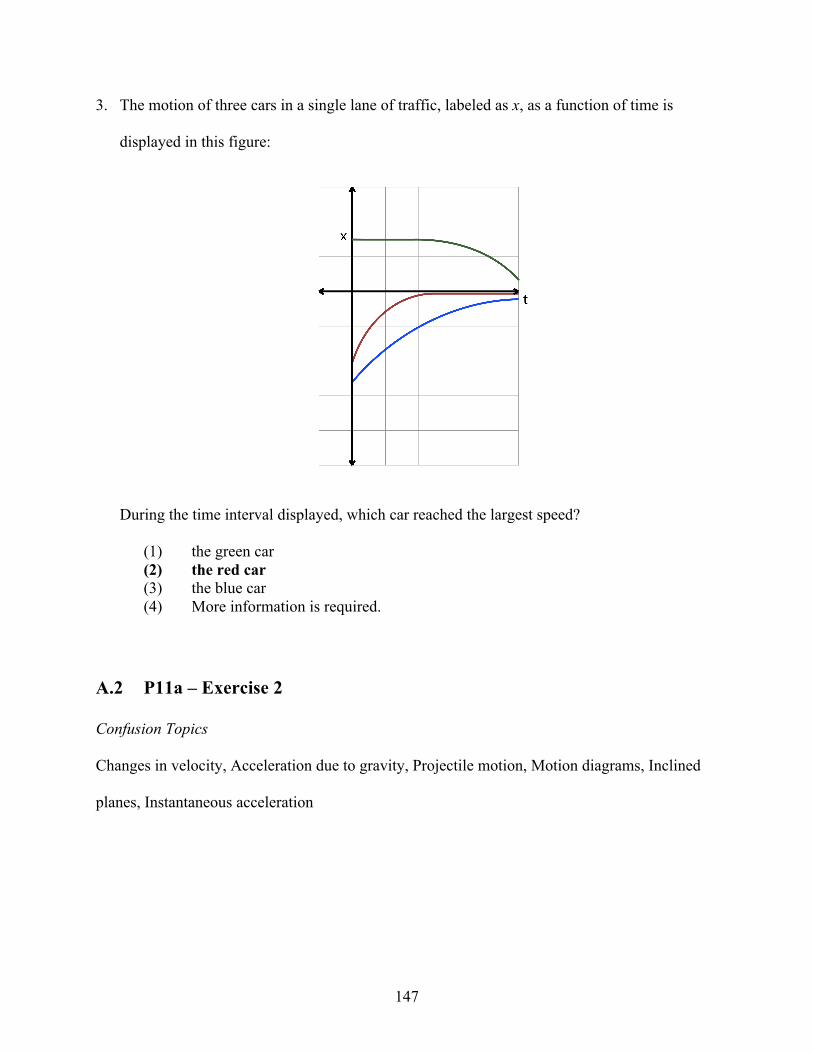
147
3. The motion of three cars in a single lane of traffic, labeled as x, as a function of time is
displayed in this figure:
During the time interval displayed, which car reached the largest speed?
(1) the green car (2) the red car (3) the blue car (4) More information is required.
A.2 P11a – Exercise 2
Confusion Topics
Changes in velocity, Acceleration due to gravity, Projectile motion, Motion diagrams, Inclined
planes, Instantaneous acceleration
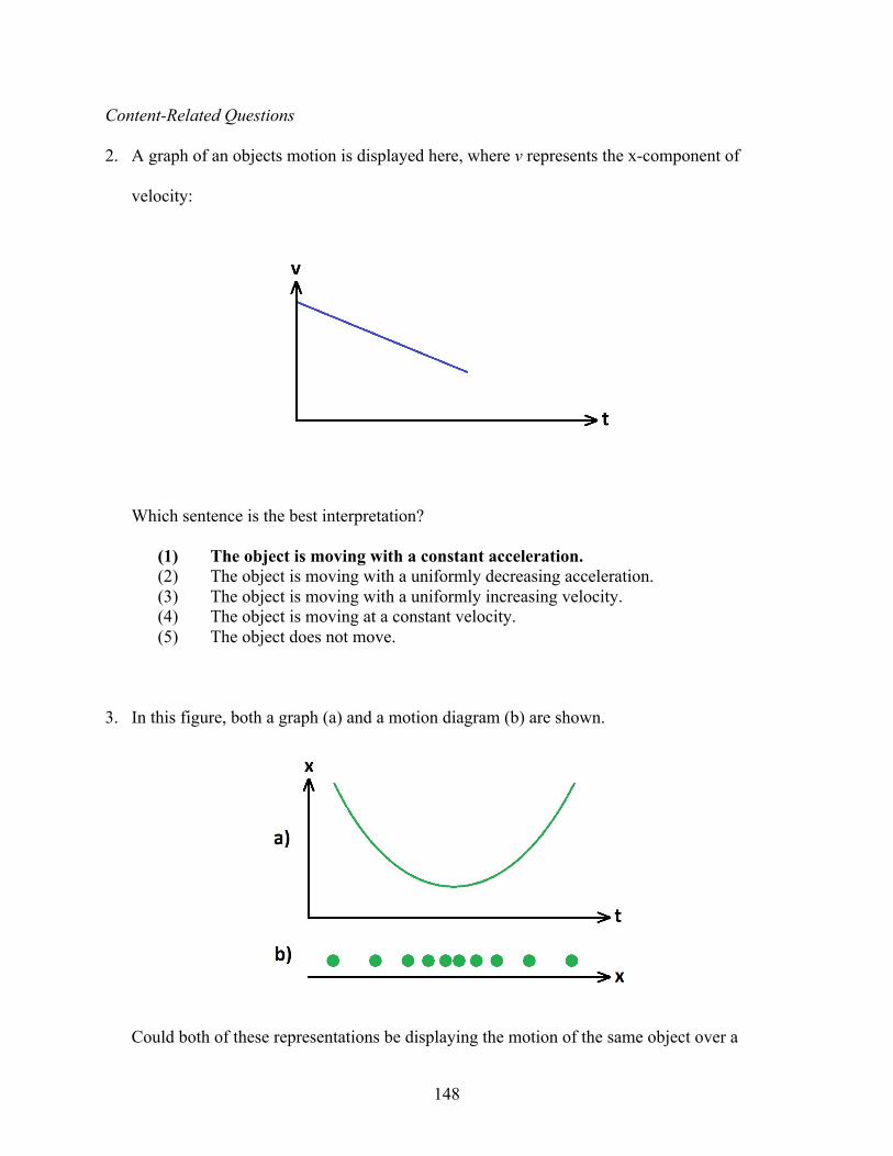
148
Content-Related Questions
2. A graph of an objects motion is displayed here, where v represents the x-component of
velocity:
Which sentence is the best interpretation?
(1) The object is moving with a constant acceleration. (2) The object is moving with a uniformly decreasing acceleration. (3) The object is moving with a uniformly increasing velocity. (4) The object is moving at a constant velocity. (5) The object does not move.
3. In this figure, both a graph (a) and a motion diagram (b) are shown.
Could both of these representations be displaying the motion of the same object over a

149
specific time interval?
(1) yes (2) no (3) Impossible to say without more information.
A.3 P11a – Exercise 3
Confusion Topics
Friction, Inertia, Systems, Momentum, Isolated systems, Conservation of momentum
Content-Related Questions
2. You are standing on the surface of the moon, where there is no atmosphere (and, therefore,
no air resistance). There is a gravitational attraction between the moon and objects on the
surface. If you are holding a heavy moon rock and a feather, and you want to throw one of
them as high as possible, which one should you throw?
(1) the feather (2) the moon rock (3) It does not matter; they will both reach the same height.
3. Paintball, if you don't happen to know, is a game in which players on opposing teams fire
small paint-filled pellets at one another. If you get hit on your bare arm with a pellet during
paintball, which of these scenarios would cause the least amount of pain?
(1) The pellet bounces off of you after striking. (2) The pellet breaks against you after striking. (3) Both scenarios would cause equal amounts of pain. (4) Either scenario could cause the least amount of pain.

150
A.4 P11a – Exercise 4
Confusion Topics
Classification of collisions, Kinetic energy, Internal energy, Closed systems, Elastic collisions,
Inelastic collisions, Conservation of energy, Explosive separations
Content-Related Questions
2. A metal ball with some initial speed (relative to the stationary table upon which this is all set
up) moves toward a magnet. The magnet is set up so that there are two identical metal balls
on the other side of the magnet (as pictured). The incoming metal ball is attracted to the
magnet (think about refrigerator magnets), so the speed of the ball increases closer to
collision (the magnet, too, is pulled toward the ball). After collision, the incoming metal ball
sticks and the second of the two additional metal balls flies off (as pictured). The final speed
of this ejected metal ball is greater than the initial speed of the incoming metal ball. We can
ignore any effects of friction.
Which of the following statements is true?
(1) The internal energy of the final system is greater than the internal energy of the initial system.

151
(2) The internal energy of the final system is less than the internal energy of the initial system.
(3) The internal energy of the final system is equal to the internal energy of the initial system.
(4) This situation is not possible; the second ball must be moving at a speed lesser than or equal to the initial speed of the incoming ball.
3. Two identical carts moving on a frictionless track collide. When I measure the relative
speeds before and after collision, the values appear to be equal. However, I had placed a
small dab of paint on one cart, and during the collision some of the paint transferred to the
other cart (so if I played a recording of the collision in reverse, it would be obvious).
Which of the following is true?
(1) The collision was elastic, but not exactly reversible in this case. (2) The collision was inelastic, but the change in velocities was very small. (3) The collision was elastic, and the paint does not matter (it is superficial). (4) The collision was inelastic, but the relative velocities did not happen to change in
this case.
A.5 P11a – Exercise 5
Confusion Topics
Relativity of motion, Inertial reference frames, Principle of relativity, Zero-momentum reference
frame, Galilean relativity, Center of mass, Convertible kinetic energy, Conservation laws and
relativity
Content-Related Questions
2. You throw a ball in the air as hard as you can and note the time at which it stops
instantaneously and reverses direction. While you are doing this, a spectator being lifted on a
hydraulic platform at a constant speed also notes the time at which the ball stops

152
instantaneously and reverses direction. Is the time reported by the spectator earlier, later, or
the same as the time you report?
(1) Spectator notes an earlier time. (2) Spectator notes a later time. (3) Spectator notes the same time as you.
3. Is there a reference frame in which the kinetic energy of a system (the whole system – not an
individual part of a system) is at a minimum? Is there a frame in which the kinetic energy of
a system is at a maximum?
Please note that this question refers to any system -- question 3 is not explicitly linked to
question 2.
1) The kinetic energy can be as low as zero or high as infinity; no limits. 2) There is a maximum kinetic energy, but the minimum could always be zero in
some frame. (3) There is a minimum, but the maximum could always be infinity in some
frame. (4) There are limits to both the minimum and maximum kinetic energy. (5) The kinetic energy of the system is constant, regardless of frame.
A.6 P11a – Exercise 6
Confusion Topics
Effects of interactions, Potential energy, Energy dissipation, Source energy, Interaction range,
Fundamental interactions, Interactions and acceleration, Nondissipative interactions, Dissipative
interactions
Content-Related Questions
2. Which of the following scenarios fit(s) with the energy bars shown here?

153
(1) A person coasting (no brakes) downhill on a bike. (2) A person parachuting from a plane at terminal (constant) speed. (3) A person climbing a ladder at a constant speed. (4) A person riding a moving walkway at the airport. (5) None of the above.
3. In class, we saw that a fan on a cart that is blowing against a barrier that is also fixed on the
same cart generates no motion. We also learned, however, that a person on a platform
throwing balls against a barrier that is fixed on the same platform does generate motion.
Which of the following scenarios, if carried out on the platform with the barrier, would
generate motion?
(1) Sandblasting the barrier. (2) Throwing socks filled with nickels at the barrier. (3) Spraying the barrier with a fire hose. (4) All of the above. (5) None of the above.
A.7 P11a – Exercise 7
Confusion Topics
Momentum and force, Reciprocity of forces, Identifying forces, Translational equilibrium, Free-

154
body diagrams, Springs and tension, Equation of motion, Force of gravity, Hooke's Law,
Impulse, Two interacting objects, Many interacting objects
Content-Related Questions
2. When I push a crate across the floor and the crate is accelerating, which force is greater in
magnitude?
(1) The force I am applying to the crate. (2) The force the crate is applying to me. (3) Neither is greater; both forces are equal. (4) More information is needed to say for sure.
3. I am hanging from a spring (a fairly heavy-duty spring, so I am definitely in the elastic
region), and the spring is attached to the ceiling by a somewhat flimsy hook. In fact, the hook
seems to just barely hold up when I am hanging perfectly still on the spring. What will
happen when I start to squirm and bounce on the spring? What would happen if it were a
rope instead of a spring (assuming the rope and the spring weigh the same, so the hook is
barely holding up in just the same way)?
(1) The hook will break, whether it is a rope or a spring. (2) The hook will break when there's a spring, but hold when there's a rope. (3) The hook will break when there's a rope, but hold when there's a spring. (4) The hook will hold, whether it is a rope or a spring. (5) We need more information.
A.8 P11a – Exercise 8
Confusion Topics
Force displacement, Positive and negative work, Energy diagrams, Choice of system, Work done
on a single-particle system, Work done on a many-particle system, Variable and distributed

155
forces, Power
Content-Related Questions
2. You throw an egg up in the air, and then you catch it. What can you say about the net work
that was done on the egg during this process?
(1) The net work done on the egg was positive. (2) The net work done on the egg was negative. (3) The net work could have been positive or negative. (4) No net work was done on the egg. (5) I cannot say anything without more information.
3. You are pushing a cart up a hill. If you choose to follow the path that switches back and forth
across the hill, rather than pushing the cart straight up the slope, what exactly are you
minimizing? Assume that you would be travelling at the same pace, regardless of the path
that is chosen.
(1) The work that you do on the cart. (2) The work that Earth (gravity) does on the cart. (3) The total source energy (from your muscles) that you expend. (4) The average power that you expend. (5) The average kinetic energy of you and the cart.
A.9 P11a – Exercise 9
Confusion Topics
Straight is a relative term, Vectors in a plane, Decomposition of forces, Friction, Work and
friction, Vector algebra, Projectile motion in two dimensions, Work as the product of two
vectors, Coefficients of friction

156
Content-Related Questions
2. Three swimmers who all swim at the same speed jump into a fast flowing river at the same
time. Swimmer A aims straight across but ends up downstream. Swimmer B aims at an
upstream angle such that he will reach the other side directly across from where he starts.
Swimmer C aims at a downstream angle, along with the current. If they all start right away,
which swimmer gets across first?
(1) Swimmer A (2) Swimmer B (3) Swimmer C (4) All three will tie. (5) Two of the three will tie.
3. Which of the following balls would you expect to travel the farthest before coming to rest
(assume they all start with the same speed, and they all eventually come to rest)?
(1) a rubber ball rolling on a basketball court (2) a rubber ball rolling on a hockey rink (3) a rubber ball skidding on a hockey rink (4) Both of the rolling balls will travel equally farther than the skidding ball. (5) All three will come to rest at the same distance.
A.10 P11a – Exercise 10
Confusion Topics
Circular motion at constant speed, Forces and circular motion, Rotational inertia
Content-Related Questions
2. You notice that, as you are copying a CD onto your computer, the rate at which it copies
increases as the transfer progresses. You know that the first track of the CD is on the

157
innermost part of the disc. You also know that the recording mechanism is a laser that moves
radially inward/outward as the disc spins. So as the transfer progresses and the laser moves
radially outward, what can you say about the rotational velocity of the CD?
(1) The rotational velocity is increasing. (2) The rotational velocity is constant. (3) The rotational velocity is decreasing. (4) The rotational velocity is constant or increasing, but not decreasing. (5) We cannot say; we need more information.
3. You swing a heavy ball in a vertical circle motion using a lightweight rope at a constant
rotational velocity. Where in the path is the rope the most likely to break?
(1) At the top of the circle. (2) At the bottom of the circle. (3) Somewhere along the upward path. (4) Somewhere along the downward path. (5) Position along the path doesn't matter; only rotational velocity matters.
A.11 P11a – Exercise 11
Confusion Topics
Rotational kinematics, Angular momentum, Rotational inertia of extended objects
Content-Related Questions
2. Two hockey sticks are at rest on an ice rink. One is pinned to the ice (a spike through the
blade into the ice holds it in place, but the stick can rotate freely), and one is sitting freely on
the ice. If a puck slides in and hits the handle of the free stick, is momentum conserved (by
"conserved" I mean "approximately conserved" -- we know that ice is not perfectly
frictionless, but that's not the effect we're interested in here)? How about angular

158
momentum? What if the puck hits the pinned stick?
(1) Both momentum and angular momentum are conserved, regardless of whether the stick is pinned.
(2) Only momentum is conserved with the free stick, and only angular momentum is conserved with the pinned stick.
(3) Angular momentum is conserved in both cases, though momentum is conserved with the free stick.
(4) Momentum is conserved in both cases, though angular momentum is conserved with the pinned stick.
(5) Neither momentum nor angular momentum is conserved in either case.
3. You are on one of those miniature merry-go-rounds at a park; it doesn’t have a motor, but a
friend pushes you up to speed by holding on and running around it. The merry-go-round is
not very big, and it doesn’t weigh much more than you. Once it is up to speed, your friend
stops pushing. Your feet are just barely gripping the surface (as in, the force of friction is
near its max) when you are standing near the outer edge. As you begin to walk and make
your way inward...
(1) You will remain very close to slipping the entire time, but you won't slip. (2) It will become easier to avoid slipping; the force of friction will no longer be near
its max. (3) You will slip. (4) More information is needed.
A.12 P11a – Exercise 12
Confusion Topics
Torque and angular momentum, Free rotation, Extended free-body diagrams, The vectorial
nature of rotation

159
Content-Related Questions
2. When you drop a wrench (or anything, really) from some height, you can impart some
rotation on that wrench. This means that some parts of the wrench are going to move upward
relative to other parts of the wrench. However, is it possible to impart enough rotation so that
some parts of the wench actually move upward as it falls in your "ground" frame of
reference?
(1) No. From the ground, even though it is rotating, all parts of the wrench always move downward.
(2) Some parts of the wrench may be moving upward from the ground, but this is not necessarily true.
(3) Yes. If the wrench is rotating, some parts of it must be moving upward.
3. You are trying to tighten a nut as much as possible using a wrench (either with or without an
extension rod), and you are considering the four configurations pictured below:
How do these configurations rank, from most successful to least successful, when it comes to
tightening the nut?
(1) All configurations are equally successful. (2) 1,2, and 4 are equally better than 3. (3) 2 and 4 are equally better than 1 and 3.

160
(4) 2 is the best, 4 is less successful, 3 is even worse, and 1 is the worst. (5) 2 is the best, 1 and 4 are equally less successful, and 3 is the worst.
A.13 P11a – Exercise 13
Confusion Topics
Conservation of angular momentum, Rolling motion, Torque and energy, The vector product
Content-Related Questions
2. When you press down on the gas pedal while driving a car, assuming the tires do not slip, is
there a friction force acting on the tires as you speed up? Is there a friction force when you
are driving at a constant velocity (still pressing the gas, though, to maintain speed)? Is there a
friction force when you are coasting (no longer pressing the gas pedal, and therefore
gradually slowing down)?
(1) No friction force in any case. (2) No friction force at constant velocity, but yes in other cases. (3) No friction force while coasting, but yes in other cases. (4) No friction forces at constant velocity or while coasting, but yes when speeding
up. (5) Yes, there is a friction force in all cases.
3. What happens when you lean to the right while riding a bicycle?
(1) You apply a torque that makes the bike speed up. (2) You apply a torque that makes the bike turn right. (3) You apply a torque that makes the bike tip over to the right. (4) You apply a torque that makes the bike tip over to the left. (5) Nothing happens; no torque is applied.

161
A.14 P11a – Exercise 14
Confusion Topics
Universal gravity, Gravity and angular momentum, Weight, Principle of equivalence,
Gravitational constant, Gravitational potential energy, Celestial mechanics, Gravitational force
exerted by a sphere
Content-Related Questions
2. When you throw a ball from the roof of a building to the ground below, what is the trajectory
that it takes?
(1) hyperbola (2) parabola (3) ellipse (4) It depends on the initial speed. (5) It depends on the initial toss angle.
3. Suppose that there exists a planet just as large as the Earth, but it is hollow and all of its mass
is condensed to a thin, uniform spherical shell. If you are on the inside of this planet, where
does the gravitational force direct you?
(1) It forces me toward the center of the hollow sphere. (2) It forces me toward the nearest surface of the hollow sphere. (3) There is no net gravitational force. (4) It forces me toward the far side of the hollow sphere. (5) More information is needed.
A.15 P11a – Exercise 15
Confusion Topics
Time measurements, Simultaneous is a relative term, Space-time, Matter and energy, Time

162
dilation, Space contraction
Content-Related Questions
2. Imagine you are driving away from a clock tower in a car that is accelerating and moving
really, really fast. As you continue to increase your speed, you observe that the clock is
ticking more and more slowly. Consider these two statements:
A) You observe the clock slowing down because the light takes longer to reach you as you
drive away.
B) You observe the clock slowing down because the time passes more slowly at the tower as
you drive away.
Which of the following is true?
(1) Statement A is true, but statement B is false. (2) Statement A is false, but statement B is true. (3) Both statements are different ways of describing the same effect, so both are true. (4) Both statements describe different effects, and both are true. (5) Both statement A and statement B are false.
3. Consider a system of three particles. Two particles are tethered together by a spring, and they
are bouncing back and forth with respect to one another (so the spring is compressed and
extended periodically). Thus, the internal energy is changing. The third particle is off to one
side, away from the particle-spring system. When you consider relativistic effects, is the
center of mass of this three-particle system changing with the oscillation?
(1) Yes, the center of mass is changing periodically. (2) No, the center of mass is not changing. (3) Maybe it changes, but it depends on the position of the third particle. (4) Maybe it changes, but it depends on the inertia of each particle in the particle-
spring system. (5) Maybe it changes, but it depends on the inertia of the third particle.

163
A.16 P11a – Exercise 16
Confusion Topics
Conservation of momentum, Conservation of energy
Content-Related Questions
2. We know that a particle cannot move at a velocity larger than c, the speed of light in vacuum.
Is there a "maximum momentum" of this particle that an observer can measure? Of course,
there could be experimental factors that limit measurement, but here we are focusing on
theoretical limits.
(1) No, there is no maximum momentum. (2) Yes, there is a maximum momentum. (3) There could be a maximum, depending on the speed of the observer. (4) There is no maximum momentum, but there is a theoretical limit to what can be
measured by an observer. (5) There is a maximum momentum, but an observer will not be sensitive to this limit
through measurement.
3. You know that hydrogen and oxygen can naturally occur as molecular hydrogen (H2),
molecular oxygen (O2), and water (H2O). You are trying to figure out whether it makes
more sense for a battery to generate power by turning molecular hydrogen and oxygen into
water, or by turning water into molecular hydrogen and oxygen. At the very minimum, what
do you need to measure?
(1) You must measure the mass of molecular hydrogen, molecular oxygen and water.
(2) You must measure the mass of molecular and atomic oxygen. (3) You must measure the mass of atomic (not molecular) hydrogen and oxygen. (4) You must measure all masses: atomic hydrogen and oxygen, molecular hydrogen
and oxygen, and water.
164
(5) You don't need to measure any masses to answer this question.
A.17 P11a – Exercise 17
Confusion Topics
Periodic motion and energy, Simple harmonic motion, Fourier's theorem, Restoring forces in
simple harmonic motion, Energy of a simple harmonic oscillator, Simple harmonic motion and
springs, Restoring torques, Damped oscillations
Content-Related Questions
2. You have a grandfather clock, but it is running a bit slowly because the pendulum takes
longer than one second to swing back and forth. You cannot shorten the pendulum (it is
hanging from a stiff rod, not a string), but you have an additional mass that you can clamp
anywhere along its length. Could adding this mass possibly fix the clock?
(1) Yes, clamping the mass to the pendulum could fix the clock. (2) No, clamping the mass to the pendulum will not affect the clock. (3) No, clamping the mass to the pendulum will further slow the clock. (4) There's no way to know how the mass will affect the clock without more
information.
3. You are trying to measure the mass of a block by hanging it from the ceiling on a spring with
a known spring constant and measuring the frequency of oscillation. You know, however,
that there is going to be some (perhaps small, but still present) effect of air resistance. Does
this affect your measurement?
(1) Yes, this means that I will only be able to set a lower limit on the mass. (2) Yes, this means that I will only be able to set an upper limit on the mass. (3) Yes, this affects the measurement, but it is impossible to determine whether the

165
measurement is high or low. (4) No, this does not affect the measurement.
A.18 P11a – Exercise 18
Confusion Topics
Representing waves graphically, Wave propagation, Superposition of waves, Boundary effects,
Wave functions, Standing waves, Wave speed, Energy transport in waves, The wave equation
Content-Related Questions
2. When you pluck a single guitar string so that a single note is produced (in other words, one
frequency dominates any higher harmonics), and you can hear this note from across the
room, is this an example of how energy is transported down the string?
(1) Yes, it is. (2) It can be, depending on the note. (3) It can be, as long as the higher harmonics are small enough. (4) No, it is not. (5) It is impossible to determine this.
3. You are looking at a snapshot of a standing wave on a rope, but at this particular instant the
rope is totally straight. From the picture, is it possible for you to identify the nodes along this
rope? If not, what would you need to know?
(1) It is possible to identify the nodes. (2) The total energy of the wave must be known to find the nodes. (3) The tension and mass density of the rope must be known to find the nodes. (4) The energy, tension and mass density all must be known to find the nodes. (5) Even with all of this information, it is not possible to find the nodes.

166
A.19 P11a – Exercise 19
Confusion Topics
Wavefronts, Sound, Interference, Diffraction, Intensity, Beats, Doppler effect, Shock waves
Content-Related Questions
2. In a concert hall, you are worried about “dead spots,” or places where the audience won’t be
able to hear all of the sounds from the stage because of destructive interference. Will hanging
carpets on the walls (which absorb and dampen sound) help eliminate dead spots?
(1) No, carpets will only reduce the volume even further. (2) No, carpets won't affect dead spots one way or the other. (3) Some carpets could help, but some carpets could exacerbate the problem. (4) Carpets may help, but they definitely won't make the dead spots worse. (5) Yes, carpets will definitely help eliminate dead spots.
3. On a particular street, there is a very narrow alley that opens onto a wide street (as shown in
the following figure).
In one situation, you are parked down the street and a squad car (with sirens blaring) is
parked in the alley. In another situation, you and the squad car have swapped: the squad car
(again, sirens blaring) is parked down the street while you are parked in the alley. In which of
these two situations will you hear the sirens most clearly?

167
(1) You'll hear the sirens best when you are in the alley. (2) You'll hear the sirens best when you are in the street. (3) You'll hear the sirens equally well in both situations. (4) You cannot hear the sirens in either situation. (5) It's impossible to determine how you will hear the sirens.
A.20 P11a – Exercise 20
Confusion Topics
Forces in a fluid, Buoyancy, Fluid flow, Surface effects, Pressure and gravity, Working with
pressure, Bernoulli's law, Viscosity and surface tension
Content-Related Questions
2. You have two different balloons. You inflate both of them as much as you possibly can (until
your lungs can't push any more air inside the balloons), and you find that one balloon is
clearly much bigger than the other. You then connect the balloons to each end of a straw that
you've clamped in the middle. Which way will air flow once you remove the clamp?
(1) Air will flow from the large balloon to the small one. (2) Air will flow from the small balloon to the large one. (3) No air flows between the balloons. (4) More information is needed to determine how the air flows.
3. There are two beakers, one filled with water and the other filled with vegetable oil. When
you put a particular ball in the water, it just barely floats (as in, only a small fraction of the
ball is above the surface of the water). When you put the same ball in the oil, it sinks to the
bottom.
What happens when you put the ball in the water, and then you pour the vegetable oil on top?
(1) The ball will remain floating at the same exact height.

168
(2) The ball will float lower, just barely touching the oil-water interface. (3) The ball will float higher, still partially within the water. (4) The ball will sink to the bottom of the water. (5) This cannot be determined from the given information.
A.21 P11a – Exercise 21
Confusion Topics
States, Equipartition of energy
Content-Related Questions
2. Which is more probable, a macrostate in which one particular particle has all of the energy or
a basic state in which each particle has an equal fraction of the energy?
(1) The macrostate is more probable than the basic state. (2) The basic state is more probable than the macrostate. (3) Both states are equally probable. (4) It is impossible to determine this with only the given information.
3. There are five particles bouncing around in a box. The total energy of all the particles is 10
units. If you track one particle over a long time, what energy is it going to have most of the
time?
(1) 0 units (2) 1 unit (3) 2 units (4) 2.5 units (5) 10 units
169
A.22 P11a – Exercise 22
Confusion Topics
Equipartition of space, Evolution toward the most probable macrostate
Content-Related Questions
2. I have a box that I’ve arbitrarily divided into four equal quadrants. I put 8 pennies in
quadrant, and then I leave the system alone for a really, really long time. When I come back
(maybe years later), how many pennies am I most likely to find in that initial quadrant?
(1) 8 pennies (2) somewhere between 2 and 8 pennies (3) 2 pennies (4) somewhere between 0 and 2 pennies (5) More information is needed.
3. Which of the following processes occur because the system is evolving toward the most
probable macrostate? Choose all that apply.
(1) Water freezing into an ice cube. (2) Water freezing into an ice cube, and the surrounding air that is warming up. (3) A refrigerator cooling the interior air by heating up the exterior air. (4) Water falling from one height to a lower height. (5) None of the above.
A.23 P11b – Exercise 1
Confusion Topics
Static electricity, Electrical charge, Mobility of charge carriers, Charge polarization, Coulomb's
law, Force exerted by distributions of charge carriers

170
Content-Related Questions
2. Positively charged sphere B is placed between two neutral metal spheres A and C, which are
connected by metal wire to a metal base, as shown in the figure below.
The connections between A and C and the metal base is cut. When sphere A is then brought
close to initially-neutral electroscope 1 and sphere C touches the top of initially-neutral
electroscope 2, what type of charge does each of the electroscopes carry?
(1) Electroscope 1 carries a positive charge, and electroscope 2 carries a negative charge.
(2) Electroscope 1 is neutral, and electroscope 2 carries a negative charge. (3) Both electroscope 1 and electroscope 2 carry a negative charge.

171
(4) Both electroscope 1 and electroscope 2 are neutral. (5) We cannot know the charges without more information.
3. Four charged particles, each of the same magnitude, with varying signs are arranged at the
corners of a square, as shown. Which of the arrows -- labeled A, B, C, and D -- gives the
correct direction of the vector sum of the forces exerted on the particle at the upper-right
corner?
(1) A (2) B (3) C (4) D (5) The vector sum of the forces is zero.
A.24 P11b – Exercise 2
Confusion Topics
The field model, Electric field diagrams, Superposition of electric fields, Electric fields and
forces, Electric field of a charged particle, Dipole field, Electric fields of continuous charge
distributions, Dipoles in electric fields

172
Content-Related Questions
2. The thin rod of length L depicted below has a charge density, λ, that varies along the rod
according to λ=bx2, where b is a positive constant.
Which of the following diagrams could represent the direction of the electric field at point P?
(1) A (2) B (3) C (4) D (5) E
3. A charged particle is released from rest in a region of uniform electric and gravitational
fields. The electric field is directed perpendicular to the gravitational field, and the
acceleration of the particle due to the electric field is comparable in magnitude to that due to
the gravitational field. Which of the following describes the trajectory of the particle in the
combined electric and gravitational fields?
(1) straight trajectory, constant velocity (2) parabolic trajectory, constant along electric field and accelerating along
gravitational field

173
(3) parabolic trajectory, accelerating along electric field and constant along gravitational field
(4) straight trajectory, accelerating (5) none of the above
A.25 P11b – Exercise 3
Confusion Topics
Electric field lines, Field line density, Closed surfaces, Symmetry and Gaussian surfaces,
Charged conducting objects
Content-Related Questions
2. Consider a field line pattern like the one shown in Figure 24.2 (reproduced below).
Suppose a negatively charged particle is released from rest from a point on one of the field
lines near the top of the diagram. After release, the particle moves...
(1) along the same direction as the field line. (2) along the field line, but in the opposite direction. (3) straight toward the negatively charged particle.

174
(4) straight toward the positively charged particle. (5) along some other trajectory.
3. Consider four charged particles, q1, q2, q3, and q4; q1 and q2 lie inside a closed surface; q3
and q4 are outside. Which particles contribute to the net flux through the closed surface?
Which particles contribute to the electric field at the surface of the closed surface?
(1) All particles contribute to the net flux and the electric field at the surface. (2) All particles contribute to the net flux; q1 and q2 contribute to the electric field at
the surface. (3) All particles contribute to the net flux; q3 and q4 contribute to the electric field at
the surface. (4) Q1 and q2 contribute to the net flux; q3 and q4 contribute to the electric field at
the surface. (5) q1 and q2 contribute to the net flux; all particles contribute to the electric
field at the surface.
A.26 P11b – Exercise 4
Confusion Topics
Electric flux, Gauss's law, Applying Gauss's law
Content-Related Questions
2. If the same amount of positive charge is distributed uniformly over two large sheets, one
conducting and one non-conducting, are the electric fields near the surface of each the same
or different?
(1) The fields are the same. (2) The field near the conducting sheet is twice as large as the field near the non-
conducting sheet. (3) The field near the non-conducting sheet is twice as large as the field near the
conducting sheet. (4) More information is needed.

175
3. A negatively charged particle is released some distance from:
1) a positively charged sphere,
2) a long positively charged rod, and
3) a large positively charged sheet.
In which of these three cases is the resulting motion of the particle one of constant
acceleration?
(1) Case 1. (2) Case 2. (3) Case 3. (4) All of the cases. (5) None of the cases.
A.27 P11b – Exercise 5
Confusion Topics
Electric potential energy, Electrostatic work, Equipotentials
Content-Related Questions
2. You want to build a new energy storage device to replace batteries. You have a special
machine that moves negatively charged particles from one stationary plate to a second plate
that is a few centimeters away. Which of the following statements is/are true?
(1) The more charged particles you move, the more energy is stored. (2) The farther the distance between the plates, the more energy is stored. (3) With each additional charged particle you move, you store even more energy than
you stored with the previous particle you moved. (4) Two of the above. (5) All of the above.

176
3. Your friend has mapped out the equipotential surfaces inside an empty box surrounded by
electronic devices. He claims that all the internal equipotential surfaces, which he measured
at regular intervals (1 V, 2 V, etc.), are flat parallel planes, but their separation is not constant
(in other words, when a test charge is moved from one end of the box to the other, its
potential energy increases more near one side compared to the other).
You know that the electronic devices around the box are creating the static electric field
inside the empty box, but you do not know the distribution of the field (as in, the distribution
of field lines). After thinking about the field lines required to achieve flat equipotential
surfaces, you realize that...
(1) ... your friend cannot be correct. (2) ... your friend must be correct. (3) ... there is no way to tell if you friend is correct without more experimentation.
A.28 P11b – Exercise 6
Confusion Topics
Calculating work and energy in electrostatics, Potential difference, Electrostatic potentials of
continuous charge distributions, Obtaining the electric field from the potential
Content-Related Questions
2. You determine the electrostatic potential at a point a certain distance away from a charge
distribution. Armed with this information, you can determine:
(1) the acceleration of an unknown charged particle at that point in space. (2) the magnitude of the electric field at that point in space. (3) the direction of the electric field at that point in space. (4) all of the above (5) none of the above
177
3. You need to calculate the electric field from a continuous charge distribution. Your friend
Amed says that it is easiest to determine the electric potential in all space and then calculate
the electric field from that. Your second friend, Beth, says that the easiest approach is to use
Gauss’ Law directly to find the electric field. Finally your third friend, Claryssa, says that
Coulomb’s Law is the most viable way. What do you think?
(1) Amed is correct. (2) Beth is correct. (3) Claryssa is correct. (4) Amed or Beth could be correct, but Claryssa is definitely wrong. (5) Any of them could be correct, depending on the charge distribution.
A.29 P11b – Exercise 7
Confusion Topics
Charge separation, Capacitors, Dielectrics, Voltaic cells and batteries
Content-Related Questions
2. Imagine bringing a positively charged rod near a metal sphere. The rod induces a polarization
in the sphere. As the rod is brought near, the electric potential energy of the system
comprised of the rod and the sphere...
(1) increases. (2) decreases. (3) stays the same. (4) The answer cannot be determined without more information.
3. A piece of dielectric material is held near a charged rod. How does the magnitude of the
electric field inside the dielectric compare to the magnitude of the electric field at the same

178
location in the absence of the dielectric?
(1) The magnitude of the electric field is the same in both situations. (2) The magnitude of the electric field is greater when the dielectric is present. (3) The magnitude of the electric field is greater when the dielectric is not
present. (4) There is no electric field inside the dielectric. (5) The answer cannot be determined without more information.
A.30 P11b – Exercise 8
Confusion Topics
Capacitance, Electric field energy and emf, Dielectric constant, Gauss' law in dielectrics
Content-Related Questions
2. Consider the insertion of a dielectric material between the plates of a fully charged parallel-
plate capacitor that is connected to a battery. What happens to the:
- capacitance (C),
- stored charge (Q),
- electric field between the plates (E) and
- potential difference in the capacitor (V)?
(1) C increases; Q, E and V remain constant. (2) C and Q increase; E and V decrease. (3) C and Q increase; E and V remain constant. (4) C, Q and E increase; V remains constant. (5) C and V remain constant; Q and E increase.
3. If you decrease the plate distance after a capacitor has been charged and disconnected from a
battery, which of the following quantities does not change?
(i) the potential change from one plate to the other;

179
(ii) the electric field line density between the plates;
(iii) the charge on each plate.
(1) I does not change. (2) II does not change. (3) III does not change. (4) II and III do not change. (5) None of them change.
A.31 P11b – Exercise 9
Confusion Topics
Magnetism, Magnetic fields, Charge flow and magnetism, Magnetism and relativity, Current and
magnetism, Magnetic flux, Moving particles in electric and magnetic fields, Magnetism and
electricity unified
Content-Related Questions
2. Two silver bars of the same size and shape are shown below. One is a bar magnet and the
other is a metal bar.
How can you identify which is the magnet?
(1) Touch (a) to (d). (2) Touch (a) to (e). (3) Touch (a) to (d), and then touch (c) to (d). (4) Simultaneously touch (a) to (d), (b) to (e), and (c) to (f), bringing them into full

180
contact. (5) With the two given objects, it's not possible to identify which is magnetic.
3. A positively-charged particle is at rest with respect to a nearby bar magnet. Depending on
your reference frame, though, both could be moving with respect to you. Which of the
following statements could be correct?
I. You measure a magnetic force on the particle that is directed along the magnetic field line
at the position of the particle.
II. You measure a magnetic force on the particle that is perpendicular to the magnetic field
line at the position of the particle.
III. You measure no magnetic force on the particle.
(1) Only I can be correct. (2) Only II can be correct. (3) Only III can be correct. (4) Perhaps I or III could be correct. (5) Perhaps II or III could be correct.
A.32 P11b – Exercise 10
Confusion Topics
Source of the magnetic field, Current loops and spin magnetism, Magnetic moment and torque,
Amperian paths
Content-Related Questions
2. A square loop of wire with sides of length L carries a current I in a clock-wise direction; the
loop is in a uniform magnetic field B that is pointing to the right, as shown.

181
What is the direction of the torque acting on the entire loop?
(1) The torque is directed up. (2) The torque is directed down. (3) The torque is directed out of the page. (4) The torque is directed into the page. (5) The torque is directed in some other direction.
3. Consider two possible Amperian paths around a wire. The first path circles around the wire
in a plane that is perpendicular to the wire. The second path is almost in the same plane as the
wire, but just barely passes on one side of the wire at one point and on the other side of the
wire at the opposite point. So both paths enclose the wire, but through very different
orientations. Which of the following statements are true?
(1) The line integrals of the magnetic field along both paths carry the same sign, but the values may be different.
(2) The line integrals of the magnetic field along each of the paths may carry opposite signs and different values.
(3) The line integrals of the magnetic field along both paths will yield the same values and carry the same signs.
(4) The line integrals of the magnetic field along both paths will yield the same values, but may carry opposite signs.
(5) None of these statements are true.

182
A.33 P11b – Exercise 11
Confusion Topics
Ampere's law, Solenoids and toroids, Magnetic fields due to currents, Magnetic field of a
moving charged particle
Content-Related Questions
2. The cable in the diagram below carries currents of equal magnitude, but opposite directions.
The magnitude of the magnetic field between the two conducting surfaces (within the
insulating sleeve) can be expressed as:
€
B = x µoIπr
⎛
⎝ ⎜
⎞
⎠ ⎟ .
What is x?
(1) The value of x is zero; there is no magnetic field. (2) The value of x is 0.5. (3) The value of x is 1. (4) The value of x is 2. (5) The value of x is not listed above.

183
3. Compare a path around a single, straight wire to a path around a wire that has been coiled
into a solenoid in the region of the loop (as shown below).
Assuming the current through each wire is the same, how do the line integrals around the
paths compare?
(1) The line integral around the straight wire is greater. (2) The line integral around the coiled wire is greater. (3) The line integrals around both wires are the same. (4) There is not enough information to make this comparison.
A.34 P11b – Exercise 12
Confusion Topics
Moving conductors in magnetic fields, Faraday's law, Electric fields accompany changing
magnetic fields, Lenz's law
Content-Related Questions
2. A neutrally-charged metal disk in a uniform magnetic field rotates about an axis that passes
through its center (as shown).

184
The potential difference of the border with respect to the center of the disk (VP - VQ) is...
(1) ... greater than zero. (2) ... less than zero. (3) ... equal to zero. (4) ... cannot be determined with the given information.
3. Imagine a large conducting loop around a very long solenoid. As you increase the current
through the solenoid, the magnetic field within the solenoid gets larger and larger. However,
the magnetic field outside of the solenoid, in the region of the conducting loop, remains
essentially zero the entire time. Is a current induced in the loop?
(1) Yes, current flows through the loop in the same direction as it flows through the solenoid.
(2) Yes, current flows through the loop in the opposite direction as it flows through the solenoid.
(3) No, there is no current in the loop. (4) This cannot be determined.
A.35 P11b – Exercise 13
Confusion Topics
Induced emf, Electric field accompanying a changing magnetic field, Inductance, Magnetic

185
energy
Content-Related Questions
2. A circular region in which there is a uniform magnetic field and a positively-charged particle
P, located out of the field, are displayed in the figure shown here.
As the magnitude of the magnetic field decreases, there is...
(1) ... a magnetic force on P. (2) ... an electric force on P. (3) ... both a magnetic and an electric force on P. (4) ... no force on P. (5) ... not enough information to determine anything about P.
3. Figure 29.33 shows two paths of integration enclosing the same area A: one circular, the
other square. Suppose these paths were replaced by a circular and a square loop of the same
shape as these two paths. If the magnetic field, B, increases at a steady rate, in which of the
two loops is the induced emf largest?
(1) The induced emf is largest in the square loop. (2) The induced emf is largest in the circular loop. (3) The induced emf is non-zero and the same in both loops. (4) The induced emf is zero in both loops. (5) This cannot be determined with the given information.

186
A.36 P11b – Exercise 14
Confusion Topics
Magnetic fields accompany changing electric fields, Fields of moving charged particles,
Oscillating dipoles and antennas
Content-Related Questions
2. The induced electric field around a changing magnetic field resists the change in magnetic
flux. How does the induced magnetic field around a changing electric field affect the change
in electric flux?
(1) The induced magnetic field around a changing electric field resists the change in electric flux.
(2) The induced magnetic field around a changing electric field amplifies the change in electric flux.
(3) The induced magnetic field around a changing electric field does not affect the change in electric flux.
(4) This cannot be determined without more information.
3. Consider a charged particle that is moving parallel to a narrow, conductive rod. Which of the
following statements is true?
(1) The electric field from a particle moving at a constant velocity can induce a current in a neighboring rod.
(2) The electric field from an accelerating particle can induce a current in a neighboring rod.
(3) The electric field from either a particle moving at a constant velocity or an accelerating particle can induce a current in a neighboring rod.
(4) None of the statements are true. (5) It is impossible to determine whether these statements are true.
187
A.37 P11b – Exercise 15
Confusion Topics
Displacement current, Maxwell's equations, Electromagnetic waves, Electromagnetic energy
Content-Related Questions
2. Suppose a dielectric is inserted between the plates of a capacitor. While the capacitor is
charging, is charge being displaced in the space between the plates? If so, is the current due
to this displacement in the same direction as the displacement current?
(1) No charge is actually displaced. (2) Charge is displaced, but it does not result in a current. (3) Charge is displaced and the current is in the same direction as the
displacement current. (4) Charge is displaced and the current is in the opposite direction as the
displacement current. (5) There is not enough information to determine this.
3. A charged particle is initially at rest in the path of a planar electromagnetic wave pulse (like
that shown in figure 30.35). When the wave first interacts with the particle, in which
direction does the resulting force on the particle point?
(1) The force points in the direction of the Poynting vector. (2) The force points in the direction of the magnetic field. (3) The force points in the direction of the electric field. (4) There is no force on the particle. (5) There is not enough information to determine the direction of the force.
A.38 P11b – Exercise 16
Confusion Topics
The basic circuit, Current and resistance, Junctions and multiple loops, Electric fields in

188
conductors
Content-Related Questions
2. Please refer to Figure 31.16 and assume that both batteries have an emf of 9 V. Suppose you
add an additional wire to connect the right terminal of bulb A to the right terminal of bulb B.
Immediately after doing this, how do the two bulbs compare to one another (assuming the
bulbs are the same)?
(1) Bulb A is brighter than bulb B. (2) Bulb B is brighter than bulb A. (3) Both bulbs are equally bright. (4) Bulb B stops emitting light. (5) Bulb A stops emitting light.
3. Consider a circuit that includes only a battery and a wire, as shown.
Assuming that the emf of the battery is constant, what happens to the magnitude of the
electric field within the wire when you increase the diameter of the wire?
(1) The magnitude of the electric field decreases. (2) The magnitude of the electric field increases.

189
(3) The magnitude of the electric field remains the same. (4) There is no electric field within the wire. (5) This cannot be determined with the given information.
A.39 P11b – Exercise 17
Confusion Topics
Resistance and Ohm's law, Single-loop circuits, Multi-loop circuits, Power in electric circuits
Content-Related Questions
2. Which of the following statements holds true inside a conductive material, when there is a
constant potential difference across the material?
I. An electric field accelerates electrons to faster and faster velocities.
II. Electrons move at a constant average velocity.
III. There are no charges inside a conductive material; charges can only exist on the surfaces.
(1) Only statement I is true. (2) Only statement II is true. (3) Only statement III is true. (4) Both statements I and II are true. (5) All three statements are true.
3. You have two identical light bulbs, two identical batteries, and some wire. Which of the
following configurations should you choose to maximize the power that is emitted from the
bulbs?

190
(1) Configuration A (2) Configuration B (3) Configuration C (4) Configuration D (5) More information is needed.
A.40 P11b – Exercise 18
Confusion Topics
Alternating currents, AC circuits, Semiconductors, Diodes; transistors and logic gates
Content-Related Questions
2. Suppose light gets absorbed in the depletion zone in Figure 32.27c (included here), causing
the separation of a hole and an electron.
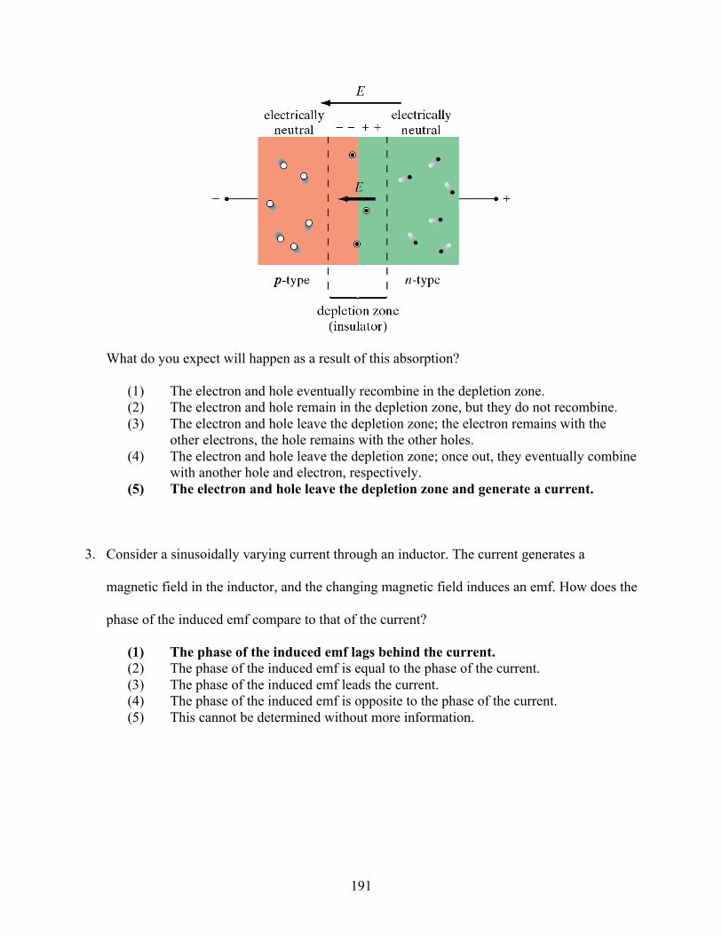
191
What do you expect will happen as a result of this absorption?
(1) The electron and hole eventually recombine in the depletion zone. (2) The electron and hole remain in the depletion zone, but they do not recombine. (3) The electron and hole leave the depletion zone; the electron remains with the
other electrons, the hole remains with the other holes. (4) The electron and hole leave the depletion zone; once out, they eventually combine
with another hole and electron, respectively. (5) The electron and hole leave the depletion zone and generate a current.
3. Consider a sinusoidally varying current through an inductor. The current generates a
magnetic field in the inductor, and the changing magnetic field induces an emf. How does the
phase of the induced emf compare to that of the current?
(1) The phase of the induced emf lags behind the current. (2) The phase of the induced emf is equal to the phase of the current. (3) The phase of the induced emf leads the current. (4) The phase of the induced emf is opposite to the phase of the current. (5) This cannot be determined without more information.

192
A.41 P11b – Exercise 19
Confusion Topics
Reactance, RC and RLC circuits, Resonance, Power in AC circuits
Content-Related Questions
2. Consider the high-pass filter shown below.
If you were to measure the output potential difference across the capacitor rather than across
the resistor, what kind of "filter" would you get?
(1) You would still have a high-pass filter. (2) You would have a low-pass filter. (3) You would have a band-pass filter (a range of frequencies can generate an output
potential difference, but not the highest or lowest frequencies). (4) All frequencies would generate an output potential difference; you would have no
filter. (5) No frequencies would generate an output potential difference; you would have no
signal.
3. Consider an RLC circuit. In each cycle, energy is stored in the capacitor, in the inductor,
retrieved from both, and dissipated in the resistor. Which of the following occur

193
simultaneously, if we apply a sinusoidal source of emf to the circuit?
A. maximum energy stored in capacitor
B. maximum energy stored in the inductor
C. maximum energy dissipated in the resistor
(1) A and B (2) A and C (3) B and C (4) A, B and C (5) None of them happen simultaneously.
A.42 P11b – Exercise 20
Confusion Topics
Rays, Absorption; transmission and reflection, Refraction and dispersion, Forming images
Content-Related Questions
2. You are standing on the bank of a pond, looking at a fish that is swimming a few feet away
from you. Compared to the actual depth at which the fish swims, is the depth at which the
fish appears to swim greater, smaller, or the same?
(1) The apparent depth is greater than the actual depth. (2) The apparent depth is smaller than the actual depth. (3) The apparent depth is the same as the actual depth. (4) This cannot be determined; more information is needed.
3. Do you need to know anything else about the following lens to determine if it is a converging
or diverging lens? Check all that apply.

194
(1) No, it is a converging lens. (2) No, it is a diverging lens. (3) We need to know the focal distance. (4) We need to know where the source has been placed. (5) We need to know the thickness at the center and edges.
A.43 P11b – Exercise 21
Confusion Topics
Snell’s law, Thin lenses and optical instruments, Spherical mirrors, Lensmaker's formula
Content-Related Questions
2. You are given a converging lens, a diverging lens, a converging mirror, and a diverging
mirror. Neglecting combinations, using which of those four can you project an image of a
pencil on a screen? Choose all that apply.
(1) a converging lens

195
(2) a diverging lens (3) a converging mirror (4) a diverging mirror (5) None of them.
3. In a combination of two lenses, would it be possible to use the second lens to make a real
image of a virtual image formed by the first lens?
(1) No, it is not possible. (2) Yes, it is possible.

196
Appendix B
Laboratory Activities
Statement about Organization (common to all laboratory activities)
One lab report should be submitted for each group (please, remember to include all names!). Lab
reports should be roughly organized as follows: statement of purpose (or statement of research
questions), hypotheses and predictions, experimental procedure, collected data, analysis of
collected data and conclusions.
Lab reports will be evaluated using rubrics that were carefully designed to assess scientific
abilities. The rubrics that will be used to evaluate this lab report are included at the end of this
document. Students are strongly encouraged to thoroughly read through these rubrics before
beginning lab reports.

197
Labs are designed to fill the entire three-hour session. It is important that you work hard and
complete as much as you can, but there is no penalty for failing to reach the “finish line.” Please
work carefully and thoroughly, and be sure to leave time at the end of the session to prepare what
you have completed for submission.
B.1 Laboratory 1 – Electric Fields, Potential Differences and
Electrocardiography
(developed from materials prepared by Catherine Crouch, Swarthmore College)
Scientific Ability Rubrics
A1, A2, A3, A4, A7, B1, B5, B6, B7, B8, B9, B10, G1, G2, G3, G4, and G5
Goals
After successfully completing this lab, you will be able to:
1) measure the electric potential of various charge distributions over an extended area,
creating a map of the potential in space
2) derive the electric field from the potential map
3) observe the electric fields generated by the human heart by measuring an
electrocardiogram
Introduction
This laboratory is divided into two parts. In the first part, you will extend your familiarity with
electric fields by exploring their connection to differences in electric potential. In the second

198
part, you will measure your electrocardiogram (ECG, or EKG [from the German
elektrokardiogramm]), which is ultimately a more sophisticated measurement of the electric
fields generated as your heart contracts and expands.
Part One
Even though we have not yet formally discussed the notion of electric potential energy, we can
begin to think about it in the same way we think of gravitational potential energy. As an object
with mass falls toward the Earth, gravitational potential energy decreases and kinetic energy
increases. Electric potential energy is the potential energy associated with the relative positions
of charged objects; as a charged particle moves through an electric field, electric potential energy
decreases and kinetic energy increases.
Mathematically, the electric field is associated with a vector function; for a given set of
coordinates, the magnitude and direction of this function gives the force per unit charge
experienced by a charged particle. The electric potential, on the other hand, is associated with a
scalar function; for a given set of coordinates, this function gives the work per unit charge
required to move a charged particle through the electric field from an arbitrary reference position
to the given coordinates. Thus, the concepts (and associated functions) are deeply related, but
quite different from one another.
To illustrate this connection (and reinforce the link between gravitational forces and
electrostatic forces), take a moment to look at the terrain maps at your table. As you remember
from P11a, gravitational potential energy changes with height: at higher elevations, the
gravitational potential energy is greater. So if you were to draw equipotential lines (that is, lines
along which the gravitational potential energy does not change), where would you draw them? If

199
you were to draw gravitational field lines, which represent the direction of the gravitational force
on a particle (or, more specifically, the net gravitational force; that is, the part that remains when
the restoring force of the Earth is taken into account), where would you draw them? What do
you notice about these equipotential and field lines?
Contours of constant height on a topographic map are analogous to contours of constant
electrostatic potential. In this lab, you will measure the equipotential contours around two or
three charge configurations, and then determine the electric field lines from the equipotential
map. The electric field and its corresponding potential are produced by distributions of charge.
Keep in mind that the (often hypothetical) particle used to measure the strength of the electric
field or potential does not contribute to the field.
The charge configurations of which you will measure the fields are shown in Figure 1. In the
laboratory, the most straightforward way to produce a distribution of charge is to use a battery or
a power supply to produce a potential difference between conducting electrodes. In the
configurations we will study, one electrode carries positive charges and the other carries negative
charges; charge is conserved in the entire system (power supply, electrodes, and ground) so the
net charge of the two electrodes together is zero. You will measure the potential of points around
the electrodes using a digital mulitmeter.
Part Two
A leading interventional cardiologist says that the electrocardiogram is the “among the most
valuable clinical tests available to medicine because it is quick, completely safe, painless,
inexpensive, and rich in information.” In part two of this lab, you’ll learn a little bit about such
measurements.

200
One’s electrocardiogram is the time-dependent potential difference that the heart generates
between selected points on the surface of the body. By measuring your EKG, you can determine
the time-dependent electric dipole moment of your heart, which results from the discharging of
the cell membranes of the cells of the heart muscle.
Why does the heart have a time-dependent electric dipole moment? The heart is made up of
muscle cells. When resting (not contracting), these cells have oppositely charged layers of ions
on either side of the cell membrane. These cells have specialized proteins that span across their
membranes called ion channels; when the cells contract, the ion channels allow positive ions to
flow into the cell and change the potential difference across the membrane (the physiological
term for this is “depolarization”). The contraction travels from cell to cell, so the edge of the
depolarized region travels across the heart.
The edge of the depolarized region has an electric field like that of an electric dipole (charges
of opposite type, separated by some distance). This edge moves as the depolarization spreads
across the heart during regular cycles of contraction and expansion. Ultimately, you will measure
the motion of this electric dipole when you measure your EKG.
Any changes in heart function, such as diseased regions of the heart muscle that fail to
contract properly, will change the moving dipole moment—hence its diagnostic utility.
Purpose
Now that you have read the introduction to this lab, please explain (in two or three sentences) the
purpose of each part of this laboratory activity. Why collect this data? What hypotheses might
you be exploring when you carry out the measurements proposed in Part One? In Part Two?

201
Procedure
Part One
In this lab you will measure equipotential lines between two parallel conducting electrodes, and
then use your measured equipotential lines to determine the electric field.
The electrodes are made using conductive tape. The strips of tape are placed on special paper
that is impregnated with carbon. While carbon is slightly conductive, it is much less conductive
than the tape that is used to make the electrodes. When the power supply is connected, charges
of opposite type collect on each of the two electrodes. Each entire electrode is essentially at the
same potential as the power supply terminal to which it is connected. Because the paper is also
conductive, charge carriers can move from one electrode to the other, from high to low potential,
just as water flows from regions of high to low gravitational potential. You might wonder why
we are measuring supposedly “static” electric fields in a configuration that involves moving
charges. Do you have any guesses about why we might do this?
To map out the equipotential lines on the paper, you will use a multimeter to measure the
potential difference between a point on the paper and a fixed reference point. To do so, simply
touch the probes firmly to the two points of interest.
There are two electrode configurations that you will be exploring in this lab: a parallel
configuration and a dipolar configuration.

202
Before measuring anything, it is important that you have make some predictions about what you
will observe…
Predictions
• Sketch the electric field lines you expect to observe from two parallel conducting sheets
when a potential difference is applied between the sheets. Remember to include the type
of charge on each sheet, and orient your sketch as a cross-section (that is, represent the
sheets as parallel lines, as in Fig. 1a).
• Then sketch the equipotential lines you expect to observe.
• Imagine a line connecting the two sheets, and sketch a graph of the electric potential vs.
position along this line, starting at the lower potential. Explain the basis for your
prediction. What does the slope of the potential vs. position graph represent?
• Repeat these sketches for the dipolar configuration.
When you have made your predictions, take a minute to chat with your TF about your
predictions. Your TF will provide two power supplies, so you can begin making measurements
after the discussion. The following procedure should be carried out for each of the two electrode
configurations. You should include a diagram of the apparatus in your report (in which all

203
connections are clearly labeled), and you should include your electrode sheet as part of the
collected data.
1. Plug the power supply into the outlet at your table and connect the leads to each of the
electrodes. Check that the potential is constant along each electrode; if it is not, ask your
TF to help cut a new set of electrodes.
2. To identify the equipotential lines, start by measuring the potential difference between
some point and your chosen reference point.
3. Record the specific value of the electric potential relative to the reference point, and then
move the probe along the paper while watching the voltmeter display; try to move the
probe along a path that keeps the potential constant.
4. While one lab partner moves the probe, another can trace the path followed by the probe
with a pencil, or mark a series of equipotential positions with dots close together and then
draw a smooth line through the dots after the path has been completed. Take turns using
the multimeter and recording the results.
5. It is impossible to keep the potential perfectly constant, so also record how much the
meter readings vary as you probe a “single” point along the path. This gives you a sense
of your measurement uncertainty.
6. After measuring one equipotential line, label that line with its potential (relative to the
reference), find a starting point that corresponds to a different potential, and start another
line. Remember to record measurements outside of the region between the electrodes, as
well. You should map equipotential lines that correspond to regular voltage intervals,
perhaps separated by 0.5 V (this is just an example; if 0.5 V results in either too many or
too few lines, choose another separation value).

204
7. Based on the equipotential map, draw in the electric field lines. Use arrows to represent
the direction.
8. Record where the field appears to be strongest and where it appears to be weakest.
Remember that the electric field is strongest where the equipotential lines are closest
together.
9. To be more quantitative, measure and record the potential (relative to the reference point)
at 0.5 cm intervals along the center line between the electrodes.
10. Use LoggerPro or Excel to plot the potential versus the distance between the electrodes,
and fit a suitable function to fit it.
You might notice that the electrodes span 12 V, but points on the paper cover a much
narrower range; this is because the adhesive between the conductive tape and the paper is not
very conductive, so the change in potential across the paper does not represent the full difference
in potential between the electrodes (there is some change in potential across the adhesive).
You are welcome to use symmetries of the electrode configuration to speed your work, but
clearly explain why you expect these symmetries to be valid. You can measure an equipotential
line carefully in one region of the paper, use symmetry to fill out the line elsewhere, and then
measure a few points to check that you are right about the symmetry. If not, can you explain the
discrepancies?
Now that you have collected data, discuss both your measurements and your predictions.
Analysis
• Are your maps and graphs of potential vs. distance consistent with your predictions? Can
you explain the differences? What information do you gain from the fit to your data?

205
• In the case of the parallel configuration, do you think the two-dimensional configuration
you measured is a reasonable model for a slice through a set of parallel plates? Why?
• Would your equipotential lines change if you had chosen a different location to serve as
the reference? If so, how would they change?
• Does the potential change as rapidly with distance in the region outside the electrodes as
it does in the region between the electrodes? Is this consistent with the electric field you
predicted?
• The SI unit for the electric field is volts/meter. Dividing the potential difference between
the electrodes by the distance between the electrodes, what is the average magnitude of
the electric field between the electrodes (with uncertainty)? Is this magnitude the same as
the slope of the potential versus distance plot? Why or why not?
Once you have finished analyzing this data, carry out the following additional measurement.
1. Construct a ring out of a single piece of conductive tape and press it down firmly between
the two electrodes already on your “parallel configuration” paper.
2. Apply a potential difference between the plate electrodes using the power supply; do not
connect anything to the ring electrode.
3. Make a prediction: do you expect the electric field lines and equipotential lines to
change? If so, how? Based on your previous measurements, what potential difference(s)
between the center disk and the reference point do you expect to measure?
4. Record and plot the potential as a function of distance along the line between the
electrodes (this line should now pass through the conducting ring), and map the
equipotential lines between the plates and the ring.

206
Further Analysis
• Compare your predicted and measured equipotential lines and electric field lines, and
explain what might have caused the differences.
• What is the electric potential inside the ring? Does it vary with position? Provide a
diagram showing how charge is distributed on the conducting ring.
• What is the electric field inside the ring? Why?
• How does the electric field outside the ring compare to the field you measured before
inserting the ring? Give a physical explanation for any difference, if you can.
• How you could estimate the strength of the electric field at a particular point on your map
based on the measured equipotential values and positions? Think about how you
calculated the electric field for the parallel electrode configuration.
Part Two
Now that you have explored the relationship between electric fields and electric potential
differences, you will carry out a measurement that has enormous utility in medicine.
Each EKG sensor has three “leads,” or wires, connected to it: red, black, and green. The
sensor measures potential difference from the green to the red lead. In other words, if the red
lead is at higher potential than the green, the reading will be positive; if the red is at lower
potential than the green, the reading will be negative. The black lead serves as the zero of
potential; when you zero the ECG sensors, the reading from the black lead is used as “zero.”
This is equivalent to the “ground” terminal on the power supplies. The black lead acts as a
reference so that multiple sensors can be used simultaneously, all with the same zero.
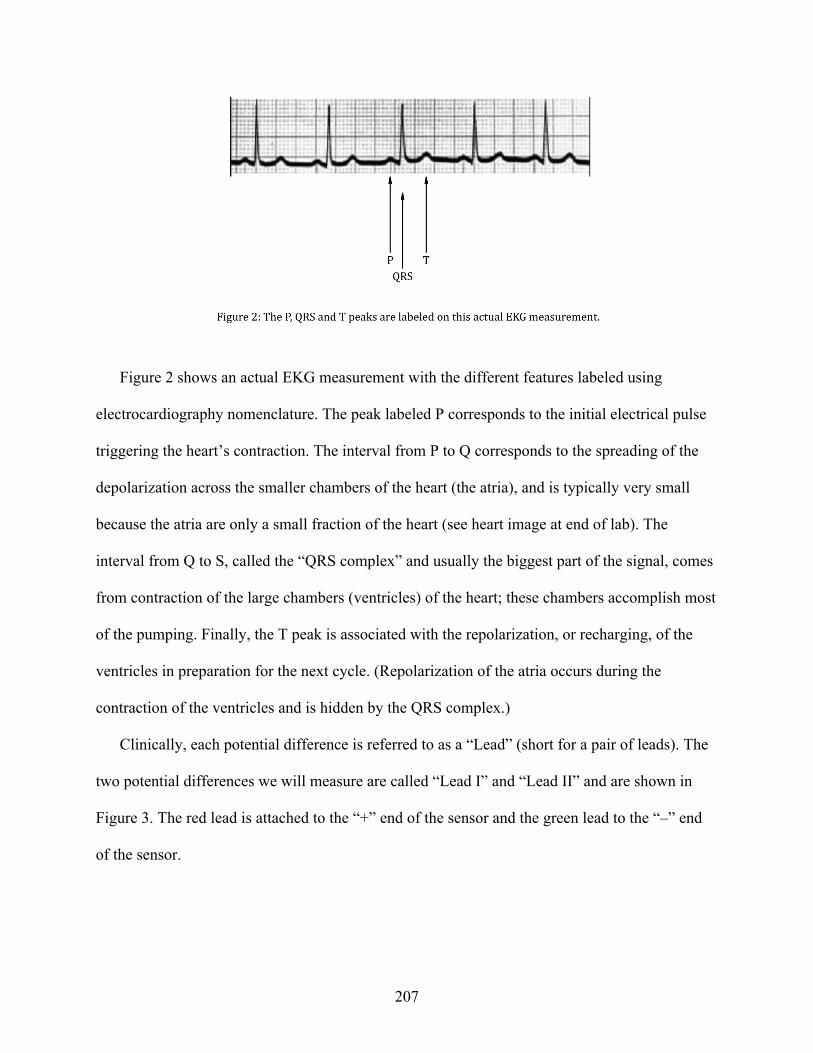
207
Figure 2 shows an actual EKG measurement with the different features labeled using
electrocardiography nomenclature. The peak labeled P corresponds to the initial electrical pulse
triggering the heart’s contraction. The interval from P to Q corresponds to the spreading of the
depolarization across the smaller chambers of the heart (the atria), and is typically very small
because the atria are only a small fraction of the heart (see heart image at end of lab). The
interval from Q to S, called the “QRS complex” and usually the biggest part of the signal, comes
from contraction of the large chambers (ventricles) of the heart; these chambers accomplish most
of the pumping. Finally, the T peak is associated with the repolarization, or recharging, of the
ventricles in preparation for the next cycle. (Repolarization of the atria occurs during the
contraction of the ventricles and is hidden by the QRS complex.)
Clinically, each potential difference is referred to as a “Lead” (short for a pair of leads). The
two potential differences we will measure are called “Lead I” and “Lead II” and are shown in
Figure 3. The red lead is attached to the “+” end of the sensor and the green lead to the “–” end
of the sensor.

208
Figure 3: These are two electrocardiography measurement configurations.
Lead I measures the potential difference between two points that fall along a horizontal line, and
thus is generated by the x-component of the dipole moment of the heart. Because of how the
heart’s electric field spreads to the limbs, the line between the Lead II points is approximately 60
degrees to the horizontal. As described further in the separate “Analysis” handout, vector
analysis allows you to combine Lead I and Lead II to determine the vertical (y-component) of the
dipole moment of the heat.
In clinical electrocardiography, twelve potential differences are measured. In this lab,
however, you will measure just two in order to determine the dipole moment of the heart in the
plane shown in Figure 3. For all measurements, the black reference lead is attached to the right
ankle. The EKG setup measures the potential difference between the red and green leads as a
function of time. You will measure both “Lead I” and “Lead II” potential differences versus time
and, from these data, determine the direction of the peak dipole moment of the heart. The ECG
measurements are made using LoggerPro.
Predictions
Do you expect “Lead I” and “Lead II” to be different from one another? In what way(s)? Why?

209
Single lead ECG measurement
1. Connect one ECG sensor to the Ch1 input on the USB interface box. The sensor should
be automatically recognized by the computer when you launch the LoggerPro software.
2. Under Experiment -> Data Collection, set the sampling rate to 250 samples/second, so
that a data point is measured every 0.004 s. Ignore Logger Pro’s warning that this is faster
than recommended.
3. The leads have so-called “alligator clips” on their end which can be clipped onto the tabs
on the sticky gel electrode patches that attach to the skin of the “patient”. Before
attaching the electrode patches, use alcohol wipes or soap and water to clean the skin
where they are to be attached, since skin oils will degrade the electrical contact.
4. One member of the lab group (the “patient”) should attach electrode patches in the four
positions (right and left ankles and right and left shoulders/upper arms) and then connect
the ECG sensor in the “Lead I” configuration (Figure 3).
5. Zero the sensor in Logger Pro and then measure an EKG.
6. Record the overall amplitude and duration of the QRS complex. The amplitude should be
a few mV and the duration should be 60-80 ms. Note that the values pointed to by the
cursor show up at the bottom of the plot itself at right, not in the large display at the
bottom-left corner.
7. Record what happens to the signal if you swap the green and red alligator clips.
Clinically, this is referred to as “lead reversal.”
8. Record what happens if the black “ground” lead is disconnected.

210
9. Switch to the “Lead II” configuration and record a single-lead EKG. Note its duration
and amplitude.
Your data should look something like those shown in Figure 2. The repetition in the signal
reflects the heart’s repeated contraction.
Peak electric dipole moment of the heart
10. Obtain a second ECG sensor and connect both “Lead I” and “Lead II” configurations
simultaneously on one person. Share sensors with another group as needed. In both cases
the black reference lead is connected in the same place.
11. Zero both sensors.
12. Measure both lead configurations simultaneously.
13. Check that the baseline level of the two signals (before the beginning of a P wave) is
close to zero; if either of the signals has a nonzero baseline, create new columns of data
in which you subtract the baseline level from the signal.
14. Calculate Lead II – (Lead I)/2 in a new column in Logger Pro (Data -> Calculate
Column) which is related to the y-component of the dipole moment. (The x-component of
the dipole moment is simply related to Lead I as discussed in the “analysis” handout.)
15. Make a new graph showing the x-component and y-component data vs. time.
Analysis
• For which of the two lead configurations is the amplitude of the QRS complex greatest?
How do the two signals differ or resemble each other?

211
• At the instant when the largest lead is at its peak, find the voltage of the other lead
configuration (not necessarily its peak).
• Use these two signals to find the direction of the electric dipole of the heart at this peak.
The electric dipole moment of the heart p is a vector; it can be written as the sum of
components, px, py, and pz. As discussed on the “analysis” handout, px and py are
proportional to the “Lead I” and “Lead II - (Lead I)/2” measurements, respectively. We
can’t easily measure the pz component of the dipole today, since you’d have to take off
your shirt to measure the voltage from front to back.
The relationships are:
Horizontal:
€
ΔVhorizontal = ΔVLead _ I =V (r,0,0) −V (−r,0,0) =px
2πε 0κwaterr2
Vertical:
€
ΔVvertical = ΔVLead _ II −Lead _ I / 2 =V (0,r,0) −V (0,−r,0) =py
2πε 0κwaterr2
For your calculations, make a reasonable estimate for the distance r from the center of the chest
cavity to the point where the potential is measured. The dielectric constant of water, κwater, is
about 80. From your data, determine px and py, and determine the magnitude and direction of
your heart’s peak electric dipole moment in the xy-plane. Do you should find a value on the order
of 10-13 Cm?
16. Make a sketch showing the orientation of your peak dipole moment on the chest
(something like the figure shown below).
How does its direction compare with the Figure 5, which shows the path followed by the dipole
moment of the heart?

212
Figure 5: Example of path followed by the tip of the cardiac dipole moment p(t) during a cardiac cycle. The vector p(t) is shown at the peak instant pointing to R. From Benedek & Villars, Physics with Illustrative Examples from Medicine and Biology, AIP Press-Springer, 2000.
Don’t forget to include…
• Written responses to all analysis questions
• Carbon paper with measured equipotential lines and electric field lines (make sure the
equipotentials are labeled with potential values)
• Plots of potential vs. distance with fits for all configurations
• Printout of the ECG data from the two simultaneous measurements
• Calculation of the magnitude and direction of heart’s dipole moment at the peak signal,
the sketch of the direction of the dipole vector on a chest, and a brief discussion of how
they compare.

213
If time permits…
Use the electrostatics simulation on the lab computer to simulate a dipole, showing both
equipotential lines and electric field vectors. Print out the result. Compare the simulation result
with your measured result. Are there any discrepancies between the simulation and your
measurements, and if so, can you account for the differences?
B.2 Laboratory 2 – Capacitance
(developed from activities in Matter and Interactions, by Ruth Chabay and Bruce
Sherwood, and materials introduced by the Rutgers Physics and Astronomy Education
Research Group)
Scientific Ability Rubrics
A7, B1, B3, B6, B7, B9, C2, C4, C5, C8, C9, D2, D7, D8, D9, F1, G1, G2, G3, G4, and G5
Goals
After successfully completing this lab, you will be able to:
1) develop hypotheses related to the charge storage properties of capacitors
2) design and carry out experiments to test such hypotheses
Introduction
This week, you will investigate the charging and discharging of capacitors. You will observe this
first qualitatively using a light bulb, and then conduct several experiments to test hypotheses and
apply what you’ve learned to discover an unknown quantity.

214
I Observational Experiment: Probing Capacitance Using a Light Bulb
Available Equipment
capacitor, batteries, wires, switch, short bulbs, long bulbs
You can certainly charge a capacitor by connecting it directly to a source of charges (a battery),
but you cannot “see” anything happening. However, with a light bulb between the battery and
the capacitor, you can see the charging much more clearly because the bulb glows when charges
are moving through the filament.
Design an experiment to investigate qualitatively how the charging and discharging of a
capacitor depends on the bulb that is connected between the capacitor and the battery.
a) Describe your experimental procedure. Include a labeled sketch. Make sure that you
identify the independent and dependent variables.
b) What assumptions are you making? Are any of them particularly questionable
assumptions? How will you minimize the effect of them?
c) Perform your experiment. Describe your observations with words and using diagrams.
d) Use your observations to determine how the charging of the capacitor depends on the
bulb that is used. Describe the reasoning you used.
e) Suggest an experiment that would allow you to investigate the same phenomenon
quantitatively. You may use equipment other than what is listed above.
215
II Testing Experiment: Differing Hypotheses about Capacitance
Available Equipment
capacitor, batteries, wires, switch, voltmeter, short bulbs, long bulbs, stopwatch
Does the final amount of charge on the capacitor plates depend on which bulb was used during
the charging process?
Your friend Andy notices that charging the capacitor through the long bulb goes on much
longer than charging through the short bulb, so he thinks that the capacitor is actually getting
charged up a lot more when the long bulb is used. Your other friend, Beth, suspects that, because
the short bulb glows much more brightly, the capacitor is getting charged up a lot more when the
short bulb is used.
Consequently, Andy hypothesizes that the capacitor carries more charge when the long bulb
is used, and Beth hypothesizes that the capacitor carries more charge when the short bulb is used.
Design a set of experiments to test Andy and Beth’s hypotheses. Remember, the goal of a
testing experiment is to disprove a hypothesis if you can. This is a significantly more powerful
step in the scientific process than merely finding another piece of supporting evidence.
Include the following in your lab report:
a) Briefly describe some (at least two) observations (involving only the available
equipment!) you would expect to make if Andy’s hypothesis were true. Similarly,
describe two observations you would expect to make if Beth’s hypothesis were true.
b) Describe your experimental procedures, which should relate to each of your observations.
Include a labeled diagram of your setup(s). Make sure that you identify the independent
and dependent variables.

216
c) What does Andy’s hypothesis predict will happen when you perform the experiment(s)?
What does Beth’s hypothesis predict will happen? This is the first part of what is known
as hypothetico-deductive reasoning: “If Andy’s idea is correct, and I do [A], then [B]
should happen.”
d) Describe any assumptions you made in making your prediction(s). How do these
assumptions affect your prediction(s)? How might they hinder your ability to make a
judgment about the hypotheses?
e) List sources of experimental uncertainty. Which are the largest? How can you minimize
them?
f) Perform the experiment and describe your results in words and with a table.
g) What is your judgment about Andy’s hypothesis? And Beth’s hypothesis? This is the
second part of hypothetico-deductive reasoning: “This did/didn’t happen, so therefore…”
III Application Experiment: Measuring Unknown Capacitance
The goal of this experiment is to determine the capacitance of an unknown capacitor.
Available Equipment
unknown capacitor, known capacitor, wires, voltmeter, battery (or power supply)
a) Devise a way to determine this and write an outline of your procedure. Include a labeled
diagram of your setup.
b) Describe the mathematical procedure you will use to determine the unknown capacitance.
Include a diagram, if needed.
217
c) List the assumptions you are making. Why do you think these assumptions are valid?
Explain how each assumption could affect the outcome (as in, will it make the measured
capacitance smaller, larger or randomly different than the actual value?)
d) List sources of experimental uncertainty. What is the largest source of uncertainty in the
result? How can you minimize it?
e) Perform the experiment. Make sure you take steps to minimize the uncertainties. Record
your observations in an appropriate format. Make a table if necessary.
f) What is the result of your experiment? How does it compare to the capacitance measured
directly using a capacitance meter? Make sure you consider uncertainty when you
compare those values.
IV Testing Experiment: Relating Parameters to Capacitance
Available Equipment
large plates, wires, capacitance meter, voltmeter, ruler, battery (or power supply)
The goal of this experiment is to test whether the rule
is applicable in this specific case. Remember that the purpose of testing is to reject (if possible),
not to support the rule under test.
Write the following in your report:
a) State what rule you are going to test.

218
b) Brainstorm the task and make a list of possible experiments whose outcome can be
predicted with the help of the rule. After making your list, discuss the options with your
TF before continuing.
c) Briefly describe your chosen design. Include a labeled sketch. Make sure that you
identify the independent and dependent variables.
d) Use the rule being tested to make a prediction about the outcome of the experiment.
Explicitly mention any assumptions you are making, and describe their effect on your
prediction.
e) List sources of experimental uncertainty. What is the largest source of uncertainty in the
result? How can you minimize it?
f) Perform the experiment. Record the outcome.
g) Is the outcome consistent or inconsistent with the prediction? Explain in detail how you
decided this.
h) Based on the prediction and outcome of the experiment, what is your judgment about the
rule being tested? Does it apply in this specific case?
i) Talk to your classmates in other lab groups and find out what results they have. Are they
consistent with yours?
Why did we do this lab?
Write a brief paragraph explaining what you have learned about capacitors in these laboratory
activities. What do you think the differences between an observational, testing and application
experiment are?
219
If time permits…
1. How bright is the bulb initially, compared to a circuit containing just a battery and a
bulb?
2. During discharging, why does the bulb get dimmer and dimmer?
3. When the light bulb is glowing, do electrons flow across the gap in the capacitor?
B.3 Laboratory 3 (scaffolded) – Magnetism
(developed from materials introduced by the Rutgers Physics and Astronomy Education
Research Group)
Scientific Ability Rubrics
A5, C1, C2, C3, C4, C5, C6, C7, C8, F1, G1, G2, G3, G4, and G5
Goals
After successfully completing this lab, you will be able to:
1) use the available equipment to design an experiment to reach a desired goal
2) apply your knowledge to solve problems in magnetism
In these laboratory activities, you will generate currents in order to observe magnetic
interactions. As Prof. [X] mentioned in class, large currents can cause significant damage to
power supplies if too much current passes through them for too long; in some cases, wires will
begin to melt and the power supply may even explode! Therefore, to limit the current flowing
through wires in this lab, make sure you include a resistor in any current loop you set up.
Resistance impedes the flow of electrons and reduces the total current through the wire. The

220
relationship between current and resistance will be further discussed in Unit 8, but it is
introduced in this lab because of the important role it plays in controlling current.
I Testing Experiment: Force on a current-carrying wire due to a magnet
Available Equipment
neodymium magnets, assorted wires, a scale, a voltage source, assorted posts and clamps, an
aluminum rod, several resistors
Think of how you can use this equipment to test the right-hand rule for the direction of the force
exerted by a magnetic field on a current carrying wire (the so-called “right-hand force rule”).
Also, think of what physical quantities you could determine using the scale.
Warning: Do not leave the voltage source on after you finish the measurements.
a) First, recall the right hand rule for the magnetic force. Write what quantities it relates and
express it with a picture or using words. Consider the available equipment and how you
could use it to achieve the goal of the experiment. Brainstorm and write down your ideas
including what you could measure and sketches of possible experimental setups.
b) Describe your procedure. The description should contain a labeled sketch of your
experimental set-up, an outline of what you plan to do, what you will measure, how you
will measure it. Explain how you will use the reading of the scale to determine the force
exerted by the wire on the magnet, and the force exerted by the magnet on the wire. To
help, use free-body diagram(s) and Newton’s second and third laws.
c) Make a qualitative prediction for the reading of the scale (more than some value, less
than some value) for your particular arrangement. Show the reasoning used to make the
221
prediction with free-body diagrams. Call your TA over once you have done this but
before you turn on the current. Then perform the experiment and record the outcome.
d) List sources of experimental uncertainty. What is the largest source of uncertainty in the
result? How can you minimize it?
e) Did the outcome match your prediction? If not, list possible reasons.
f) Based on your prediction and the experimental outcome, make a judgment about the
right-hand rule.
II Observation experiment: Invent your own investigation
Available Equipment
neodymium magnets, assorted wires, a scale, a voltage source, assorted posts and clamps, an
aluminum rod, several resistors, a variable resistor, an ammeter, shims
What mathematical relationship between physical quantities could you investigate using the
available equipment? Pose a question, investigate it, and write a brief summary of the results of
the investigation. Include a statement of the mathematical relationship you found.
III Testing experiment: Does a coil behave like a magnet?
Available Equipment
neodymium magnets, assorted wires, a voltage source, assorted posts and clamps, a coiled wire,
a compass, several resistors

222
Your friend Luis has an idea that a coil of wire with current flowing in it behaves like a bar
magnet whose poles can be determined using the right-hand current rule. Design an experiment
to test his idea.
a) First recall what the “right-hand current rule” says. Decide how you can apply it to
determine the shape of the magnetic field of a current carrying coil.
b) Design an experiment to test Luis’ idea. Describe your procedure and draw a sketch of
your experimental setup.
c) Using Luis’ idea, make a prediction of the outcome of the experiment. Explain the
reasoning used to make the prediction in detail. What assumption do you need to make
the prediction?
d) Use the wire to make a coil with several turns. Conduct the experiment and record the
outcome.
e) Did the outcome match the prediction?
f) What is your judgment about Luis’ idea?
IV Testing Experiment: Magnetic field of a current-carrying wire
Available Equipment
assorted wires, assorted compasses, a voltage source, assorted posts and clamps, a protractor,
several resistors, an ammeter
In Experiment I, you explored the relationship between force and current. Here, you will explore
the relationship between magnetic field and current. Using these materials and what you know

223
about the direction of the magnetic field around a wire, how might you be able to quantify the
strength of the magnetic field generated by a wire?
Write the following in your report:
a) State what rule you are going to test.
b) Brainstorm the task and think of some measurements you could make. Discuss the
options with your TF before continuing.
c) Briefly describe your chosen design. Include a labeled sketch. Make sure that you
identify the independent and dependent variables.
d) Use the rule being tested to make a prediction about the outcome of the experiment.
Explicitly mention any assumptions you are making, and describe their effect on your
prediction.
e) List sources of experimental uncertainty. What is the largest source of uncertainty in the
result? How can you minimize it?
f) Perform the experiment. Record the outcome.
g) Is the outcome consistent or inconsistent with the prediction? Explain in detail how you
decided this.
h) Based on the prediction and outcome of the experiment, what is your judgment about the
rule being tested? Does it apply in this specific case?
Why did we do this lab?
What was the purpose of using free-body diagrams in this lab? Describe the instances when the
diagrams helped you make decisions related to the collection of your data and the analysis.
224
What steps did you take to minimize the experimental uncertainty in the measurement of the
current in experiment II?
Why was it important to consider the assumption you made in experiment III?
B.4 Laboratory 3 (exploratory) – Magnetism
(developed from materials introduced by the University of Maryland Physics Education
Research Group)
Scientific Ability Rubrics
A5, C1, C2, C3, C4, C5, C6, C7, C8, F1, G1, G2, G3, G4, and G5
Goals
After successfully completing this lab, you will be able to:
1) use the available equipment to design an experiment to reach a desired goal
2) apply your knowledge to solve problems in magnetism
In these laboratory activities, you will generate currents in order to observe magnetic
interactions. As Prof. [X] mentioned in class, large currents can cause significant damage to
power supplies if too much current passes through them for too long; in some cases, wires will
begin to melt and the power supply may even explode! Therefore, to limit the current flowing
through wires in this lab, make sure you include a resistor in any current loop you set up.
Resistance impedes the flow of electrons and reduces the total current through the wire. The
relationship between current and resistance will be further discussed in Unit 8, but it is
introduced in this lab because of the important role it plays in controlling current.
225
Question
What is the direction of the force on a current-carrying wire due to a magnet?
Quantitatively describe the relationship between the force on the magnet and the current
through the wire. Use whatever tools and techniques you’d like, as long as they can be explained
to the rest of the class during discussion.
Available Equipment
neodymium magnets, assorted wires, a scale, a voltage source, assorted posts and clamps, an
aluminum rod, several resistors, an ammeter, shims
Warning: Do not leave the voltage source on after you finish the measurements.
Timetable
1. Pre-Lab Discussion - 20 min - Whole class
2. Planning the Experiment (Q1) - 20 min - Groups
• How are you going to illustrate your data?
• How are you accounting for uncertainty in the measurements?
• What seems to be the behavior or features of this relationship?
• How can you quantify this relationship so that it can be communicated to others?
3. Data Collecting (Q1) - 20 min - Groups
4. Class Discussion (Q1 and Q2) - 20 min - Whole Class
5. More Data Collecting (Q2) - 20 min – Groups

226
6. Data Analysis (Q1 and Q2) - 40 minutes - Groups
7. Writing the Report (Q1 and Q2) - 30 minutes - Groups
B.5 Laboratory 4 (scaffolded) – Electromagnetic Induction
(developed from materials introduced by the Rutgers Physics and Astronomy Education
Research Group)
Scientific Ability Rubrics
B2, B4, B9, C4, C6, C8, F1, and G1
Goals
After successfully completing this lab, you will be able to:
1) determine the conditions under which a current can be induced in a coil that is not
connected to a battery;
2) determine which physical quantities affect the magnitude of the induced current;
3) record data carefully and identify patterns; and
4) revise a rule when new observations are made.
In these laboratory activities, you will generate currents in order to observe magnetic
interactions. As Prof. [X] mentioned in class, large currents can cause significant damage to
power supplies if too much current passes through them for too long; in some cases, wires will
begin to melt and the power supply may even explode! Therefore, to limit the current flowing
through wires in this lab, make sure you include a resistor and a switch in any current loop you
227
connect to a voltage supply. Also, please remember to turn off voltage supplies when you are
not using them.
You will use galvanometers and voltage supplies in these activities. The galvanometer
must never be placed in the same circuit as the voltage supply; they must be completely
disconnected from one another. The galvanometer is extremely sensitive and will be instantly
damaged if it is connected to the voltage supply in any way.
I Observation experiment: Using a magnet to induce a current in a coil
Available Equipment
neodymium magnets, a coiled wire, a galvanometer, connecting wires
Your goal is to design as many experiments as possible to cause a current (also called ‘inducing
a current’) in a coil of wire that is not connected to a battery. Even though these experiments are
qualitative in nature, be specific and precise with what you do.
a) First, decide how you would set-up the experiment to detect if there is current in the coil.
Hint: The galvanometer needle will deflect if a current flows through it.
b) Draw a sketch for each experiment you perform. Briefly describe what you did. Indicate
whether there was current induced in the coil or not.
c) Develop a rule: Devise a preliminary rule that summarizes the list of conditions needed to
induce a current in a coil.

228
II Testing experiment: Does a coil behave like a magnet?
Available Equipment
two coils, assorted connecting wires, a voltage source (with resistors and switch), a galvanometer
In the previous lab you may have attempted to disprove the hypothesis that a coil of wire with
current behaves like a bar magnet. Keep trying! Design experiments using this equipment to try
to disprove this idea. Hint: Use your knowledge about the properties of magnets to induce
current in a coil using a second coil instead of a magnet.
a) Design as many experiments as you can (at least two) to test the idea.
For each experiment:
b) Describe your experimental procedure and include a labeled diagram
c) Using the idea you are testing make a prediction of the outcome of the experiment.
d) Conduct the experiment and record the outcome.
e) Did the outcome match your prediction?
What is your judgment about the idea?
III Observation experiment: Inducing a current in a coil
Available Equipment
2 coils, a voltage source (with resistors and switch), connecting wires, a galvanometer
One of the coils is connected to the voltage source, and the other is not. Your goal is to design an
experiment to induce current in the coil that is not connected to the voltage source, without
moving either coil.

229
a) Describe your experimental procedure. Include a labeled diagram.
b) Indicate whether there was current induced in the coil or not.
c) Develop a rule: Revise the rule you devised in experiment I by devising a more general
rule that summarizes the results of the observations from experiments I and III. Hint:
Think about this rule in terms of the magnetic field.
IV Observation experiment: Magnitude of induced current
Available Equipment
neodymium magnets, coils with varying number of windings, a galvanometer, a voltage source
(with resistors and switch)
By now, you know how to use a magnet to induce a current in the coil. Your goal for this set of
experiments is to devise a qualitative rule that relates the magnitude of induced current to the
properties of the magnet, the motion of the magnet, and the properties and the orientation of the
coil.
a) Briefly describe each experiment using a sketch or words.
b) Come up with as complete a list as possible of factors that affect the magnitude of the
current induced in the coil.
c) Summarize the factors that affect the magnitude of the induced current. Devise a
qualitative rule (in words) that relates the magnitude of induced current to other factors.
Hint: Think about this rule in terms of the magnetic field.

230
V How does a galvanometer work?
Available Equipment
a galvanometer
a) Play with the galvanometer.
b) Discuss how the galvanometer works with your group and with your TA.
c) Is your understanding of a galvanometer work consistent now with your previous
knowledge? If not, why?
Why did we do this lab?
Summarize your findings:
• What are the conditions under which a current can be induced in a coil that is not
connected to a battery?
• What are the factors that affect the magnitude of the induced current?
When several factors affect some physical quantity, what is the general strategy that you
would use to determine the effect of each of them?
B.6 Laboratory 4 (exploratory) – Electromagnetic Induction
(developed from materials introduced by the University of Maryland Physics Education
Research Group)
Scientific Ability Rubrics
B2, B4, B9, C4, C6, C8, F1, and G1

231
Goals
After successfully completing this lab, you will be able to:
1) determine the conditions under which a current can be induced in a coil that is not
connected to a battery;
2) determine which physical quantities affect the magnitude of the induced current;
3) record data carefully and identify patterns; and
4) revise a rule when new observations are made.
In these laboratory activities, you will generate currents in order to observe magnetic
interactions. As Prof. [X] mentioned in class, large currents can cause significant damage to
power supplies if too much current passes through them for too long; in some cases, wires will
begin to melt and the power supply may even explode! Therefore, to limit the current flowing
through wires in this lab, make sure you include a resistor and a switch in any current loop you
connect to a voltage supply. Also, please remember to turn off voltage supplies when you are
not using them.
You will use galvanometers and voltage supplies in these activities. The galvanometer
must never be placed in the same circuit as the voltage supply; they must be completely
disconnected from one another. The galvanometer is extremely sensitive and will be instantly
damaged if it is connected to the voltage supply in any way.

232
Question
Describe several different ways can you induce a current in a coil. How does the magnitude of
the induced current depend on properties – position, motion, orientation, etc. – of the materials
that are used?
Available Equipment
neodymium magnets, several coiled wires, a galvanometer, a voltage source (with resistors and
switch), connecting wires
Timetable
1. Pre-Lab Discussion - 20 min - Whole class
2. Planning the Experiments - 20 min - Groups
• How are you going to illustrate your data?
• How are you accounting for uncertainty in the measurements?
• What seems to be the behavior or features of this relationship?
• How can you quantify this relationship so that it can be communicated to others?
3. Data Collecting - 20 min - Groups
4. Class Discussion - 20 min - Whole Class
5. More Data Collecting - 20 min – Groups
6. Data Analysis - 40 minutes - Groups
7. Writing the Report - 30 minutes - Groups

233
B.7 Laboratory 5 – DC Circuits
(developed from materials introduced by the University of Maryland Physics Education
Research Group)
Scientific Ability Rubrics
B7, C2, C5, C6, C7, F1, G2, and G5
Goals
After successfully completing this lab, you will be able to:
1) determine whether a particular trend is exhibited by collected data; and
2) establish a rule, based on data, and apply it when appropriate.
There are some materials that conduct electricity so that the current that flows through them is
linearly proportional to the applied voltage. Such a material is called “Ohmic.” If you know that
a material is Ohmic, you can tell what the current is just by knowing how much voltage you are
applying. Predictability is important for certain electrical hardware.
Question
Is an electrical resistor Ohmic? Is a light bulb Ohmic? Propose a “rule” that determines whether
data is linear or not. According to this rule, are any of your other materials Ohmic?
234
Available Equipment
a voltage source, an ammeter, a voltmeter, a switch, a light bulb, several resistors, connecting
wires, diode, additional wires of various types, water, salt, a beaker
Timetable
1. Pre-Lab Discussion - 20 min - Whole class
2. Planning the Experiment - 20 min - Groups
• How are you going to illustrate your data?
• How are you accounting for uncertainty in the measurements?
• What seems to be the behavior or features of this relationship?
• How can you quantify this relationship so that it can be communicated to others?
3. Data Collecting - 20 min - Groups
4. Class Discussion - 20 min - Whole Class
5. More Data Collecting - 20 min – Groups
6. Data Analysis - 40 minutes - Groups
7. Writing the Report - 30 minutes - Groups

235
Appendix C
Scientific Ability Rubrics
These rubrics were developed by and are reproduced with permission of the Rutgers Physics and
Astronomy Education Research Group.
Scoring Key
1) Missing
2) Inadequate
3) Needs some improvement
4) Adequate

236
C.1 Rubric A: Ability to represent information in multiple ways
A1 Is able to extract the information from representation correctly
1) No visible attempt is made to extract information from the problem.
2) Information that is extracted contains errors such as labeling quantities incorrectly.
3) Some of the information is extracted correctly, but not all of the information.
Numbers are just extracted with correct labels but no units are extracted with them.
4) All necessary information has been extracted correctly and is visible through a
constructed representation.
A2 Is able to construct new representations from previous representations
1) No attempt is made to construct a different representation.
2) Representations are attempted, but use incorrect information or the representation
does not agree with the information used.
3) Representations are created without mistakes, but there is information missing, i.e.
labels, variables.
4) Representations are constructed with all given (or understood) information and
contain no major flaws.
A3 Is able to evaluate the consistency of different representations and modify them when
necessary
1) No representation is made to evaluate the consistency.
2) At least one representation is made but there are major discrepancies between the
constructed representation and the given one.

237
3) Representations created agree with each other but may have slight discrepancies with
the given representation. Can be seen that modifications were made to a
representation.
4) All representations, both created and given, are in agreement with each other.
A4 Is able to use representations to solve problems
1) No attempt is made to answer the problem.
2) Question is answered incorrectly.
3) Question is answered correctly without the use of a representation.
4) Question is answered correctly with the use of a representation other then a
mathematical.
Representations students can make
A5 Free-Body Diagram
1) No representation is constructed.
2) FBD is constructed but contains major errors such as incorrect mislabeled or not
labeled force vectors, length of vectors, wrong direction, extra incorrect vectors are
added, or vectors are missing.
3) FBD contains no errors in vectors but lacks a key feature such as labels of forces with
two subscripts or vectors are not drawn from single point or axes are missing.
4) The diagram contains no errors and each force is labeled so that it is clearly
understood what each force represents.

238
A6 Motion Diagram
1) No representation is constructed.
2) Diagram does not show proper motion, because lengths of arrows are incorrect or
missing and/or spacing of dots is incorrect.
3) Diagram has no errors but is missing a key feature such as dots that represent position
or velocity arrows or velocity change arrows.
4) The diagram contains no errors and it clearly describes the motion of the object.
A7 Picture
1) No representation is constructed.
2) Picture is drawn but it is incomplete with no physical quantities labeled, or important
information is missing, or it contains wrong information, or coordinate axes are
missing.
3) Picture has no incorrect information but has either no or very few labels of given
quantities. Majority of key items are drawn in the picture.
4) Picture contains all key items with the majority of labels present.
A8 Energy Bar Chart
1) No representation is constructed.
2) Bar chart is either missing energy values, values drawn do not show the conservation
of energy or are drawn in the wrong places. Bar chart levels could also be labeled
incorrectly

239
3) Bar chart has the energy levels drawn correctly, but is missing labels. Energy levels
could be in the correct spot, but may not be of proper relative size.
4) Bar chart is properly labeled and has energy levels at appropriate magnitudes.
A9 Mathematical
1) No representation is constructed.
2) Mathematical representation lacks the algebraic part (the student plugged the numbers
right away) has the wrong concepts being applied, signs are incorrect, or progression
is unclear. The first part should be applied when it is appropriate.
3) No error is found in the reasoning, however they may not have fully completed steps
to solve problem or one needs effort to comprehend the progression.
4) Mathematical representation contains no errors and it is easy to see progression of the
first step to the last step in solving the equation.
A10 Ray Diagram
1) No representation is constructed.
2) The rays that are drawn in the representation do not follow the correct paths. Object
or image may be located at wrong position.
3) Diagram is missing key features but contains no errors. One example could be the
object is drawn with the correct lens/mirror but rays are not drawn to show image. Or
the rays are too far from the main axis to have a small-angle approximation.
4) Diagram has object and image located in the correct spot with the proper labels. Rays
are correctly drawn with arrows and contain at least two rays.

240
C.2 Rubric B: Ability to design and conduct an observational experiment
B1 Is able to identify the phenomenon to be investigated
1) No phenomenon is mentioned.
2) The description of the phenomenon to be investigated is confusing, or it is not the
phenomena of interest.
3) The description of the phenomenon is vague or incomplete.
4) The phenomenon to be investigated is clearly stated.
B2 Is able to design a reliable experiment that investigates the phenomenon
1) The experiment does not investigate the phenomenon.
2) The experiment may not yield any interesting patterns.
3) Some important aspects of the phenomenon will not be observable.
4) The experiment might yield interesting patterns relevant to the investigation of the
phenomenon.
B3 Is able to decide what parameters are to be measured and identify independent and
dependent variables
1) The parameters are irrelevant.
2) Only some of parameters are relevant.
3) The parameters are relevant. However, independent and
4) The parameters are relevant and independent and dependent
241
B4 Is able to describe how to use available equipment to make measurements
1) At least one of the chosen measurements cannot be made with the available
equipment.
2) All chosen measurements can be made, but no details are given about how it is done.
3) All chosen measurements can be made, but the details of how it is done are vague or
incomplete.
4) All chosen measurements can be made and all details of how it is done are clearly
provided.
B5 Is able to describe what is observed without trying to explain, both in words and by
means of a picture of the experimental set-up.
1) No description is mentioned.
2) A description is incomplete. No labeled picture is present. Or, observations are
adjusted to fit expectations.
3) A description is complete, but mixed up with explanations or pattern.
4) Clearly describes what happens in the experiments both verbally and by means of
other representations.
B6 Is able to identify the shortcomings in an experimental and suggest improvements
1) No attempt is made to identify any shortcomings of the experimental.
2) The shortcomings are described vaguely and no suggestions for improvements are
made.
242
3) Not all aspects of the design are considered.
4) All major shortcomings of the experiment are identified and reasonable suggestions
for improvement are made.
B7 Is able to identify a pattern in the data
1) No attempt is made to search for a pattern
2) The pattern described is irrelevant or inconsistent with the data
3) The pattern has minor errors or omissions
4) The patterns represents the relevant trend in the data
B8 Is able to represent a pattern mathematically (if applicable)
1) No attempt is made to represent a pattern mathematically.
2) The mathematical expression does not represent the trend.
3) No analysis of how well the expression agrees with the data is included, or some
features of the pattern are missing.
4) The expression represents the trend completely and an analysis of how well it agrees
with the data is included.
B9 Is able to devise an explanation for an observed pattern
1) No attempt is made to explain the observed pattern.
2) An explanation is vague, not testable, or contradicts the pattern.
3) An explanation contradicts previous knowledge or the reasoning is flawed.
4) A reasonable explanation is made.
243
B10 Is able to identify the assumptions made in devising the explanation
1) No attempt is made to identify any assumptions.
2) The assumptions are irrelevant or incorrect.
3) Some significant assumptions are not mentioned.
4) Most significant assumptions are correctly identified.
C.3 Rubric C: Ability to design and conduct a testing experiment
(testing an idea/hypothesis/explanation or mathematical relation)
C1 Is able to identify the hypothesis to be tested
1) No mention is made of a hypothesis.
2) An attempt is made to identify the hypothesis to be tested but is described in a
confusing manner.
3) The hypothesis to be tested is described but there are minor omissions or vague
details.
4) The hypothesis is clearly stated.
C2 Is able to design a reliable experiment that tests the hypothesis
1) The experiment does not test the hypothesis.
2) The experiment tests the hypothesis, but due to the nature of the design it is likely the
data will lead to an incorrect judgment.
3) The experiment tests the hypothesis, but due to the nature of the design there is a
moderate chance the data will lead to an inconclusive judgment.

244
4) The experiment tests the hypothesis and has a high likelihood of producing data that
will lead to a conclusive judgment.
C3 Is able to distinguish between a hypothesis and a prediction
1) No prediction is made. The experiment is not treated as a testing experiment.
2) A prediction is made but it is identical to the hypothesis.
3) A prediction is made and is distinct from the hypothesis but does not describe the
outcome of the designed experiment.
4) A prediction is made, is distinct from the hypothesis, and describes the outcome of
the designed experiment
C4 Is able to make a reasonable prediction based on a hypothesis
1) No attempt to make a prediction is made.
2) A prediction is made that is distinct from the hypothesis but is not based on it.
3) A prediction is made that follows from the hypothesis but does not incorporate
assumptions
4) A correct prediction is made that follows from the hypothesis and incorporates
assumptions.
C5 Is able to identify the assumptions made in making the prediction
1) No attempt is made to identify any assumptions.
2) An attempt is made to identify assumptions, but the assumptions are irrelevant or are
confused with the hypothesis.
245
3) Relevant assumptions are identified but are not significant for making the prediction.
4) All assumptions are correctly identified.
C6 Is able to determine specifically the way in which assumptions might affect the prediction
1) No attempt is made to determine the effects of assumptions.
2) The effects of assumptions are mentioned but are described vaguely.
3) The effects of assumptions are determined, but no attempt is made to validate them.
4) The effects of the assumptions are determined and the assumptions are validated.
C7 Is able to decide whether the prediction and the outcome agree/disagree
1) No mention of whether the prediction and outcome agree/disagree.
2) A decision about the agreement/disagreement is made but is not consistent with the
outcome of the experiment.
3) A reasonable decision about the agreement/disagreement is made but experimental
uncertainty is not taken into account.
4) A reasonable decision about the agreement/disagreement is made and experimental
uncertainty is taken into account.
C8 Is able to make a reasonable judgment about the hypothesis
1) No judgment is made about the hypothesis.
2) A judgment is made but is not consistent with the outcome of the experiment.
3) A judgment is made and is consistent with the outcome of the experiment but
assumptions are not taken into account.

246
4) A reasonable judgment is made and assumptions are taken into account.
C9 Is able to revise the hypothesis when necessary
1) A revision is necessary but none is made.
2) A revision is made but the new hypothesis is not consistent with the results of the
experiment.
3) A revision is made and is consistent with the results of the experiment but other
relevant evidence is not taken into account.
4) A revision is made and is consistent with all relevant evidence.
C.4 Rubric D: Ability to design and conduct an application experiment
D1 Is able to identify the problem to be solved
1) No mention is made of the problem to be solved.
2) An attempt is made to identify the problem to be solved but it is described in a
confusing manner.
3) The problem to be solved is described but there are minor omissions or vague details.
4) The problem to be solved is clearly stated.
D2 Is able to design a reliable experiment that solves the problem
1) The experiment does not solve the problem.
2) The experiment attempts to solve the problem but due to the nature of the design the
data will not lead to a reliable solution.

247
3) The experiment attempts to solve the problem but due to the nature of the design
there is a moderate chance the data will not lead to a reliable solution.
4) The experiment solves the problem and has a high likelihood of producing data that
will lead to a reliable solution.
D3 Is able to use available equipment to make measurements
1) At least one of the chosen measurements cannot be made with the available
equipment.
2) All of the chosen measurements can be made, but no details are given about how it is
done.
3) All of the chosen measurements can be made, but the details about how they are done
are vague or incomplete.
4) All of the chosen measurements can be made and all details about how they are done
are provided and clear.
D4 Is able to make a judgment about the results of the experiment
1) No discussion is presented about the results of the experiment
2) A judgment is made about the results, but it is not reasonable or coherent.
3) An acceptable judgment is made about the result, but the reasoning is flawed or
incomplete.
4) An acceptable judgment is made about the result, with clear reasoning. The effects of
assumptions and experimental uncertainties are considered.
248
D5 Is able to evaluate the results by means of an independent method
1) No attempt is made to evaluate the consistency of the result using an independent
method.
2) A second independent method is used to evaluate the results. However there is little
or no discussion about the differences in the results due to the two methods.
3) A second independent method is used to evaluate the results. The results of the two
methods are compared using experimental uncertainties. But there is little or no
discussion of the possible reasons for the differences when the results are different.
4) A second independent method is used to evaluate the results and the evaluation is
done with the experimental uncertainties. The discrepancy between the results of the
two methods, and possible reasons are discussed.
D6 Is able to identify the shortcomings in an experimental design and suggest specific
improvements
1) No attempt is made to identify any shortcomings of the experimental design.
2) An attempt is made to identify shortcomings, but they are described vaguely and no
specific suggestions for improvements are made.
3) Some shortcomings are identified and some improvements are suggested, but not all
aspects of the design are considered.
4) All major shortcomings of the experiment are identified and specific suggestions for
improvement are made.

249
D7 Is able to choose a productive mathematical procedure for solving the experimental
problem
1) Mathematical procedure is either missing, or the equations written down are
irrelevant to the design.
2) A mathematical procedure is described, but is incorrect or incomplete, due to which
the final answer cannot be calculated.
3) Correct and complete mathematical procedure is described but an error is made in the
calculations.
4) Mathematical procedure is fully consistent with the design. All quantities are
calculated correctly. Final answer is meaningful.
D8 Is able to identify the assumptions made in using the mathematical procedure
1) No attempt is made to identify any assumptions.
2) An attempt is made to identify assumptions, but the assumptions are irrelevant or
incorrect for the situation.
3) Relevant assumptions are identified but are not significant for solving the problem.
4) All relevant assumptions are correctly identified.
D9 Is able to determine specifically the way in which assumptions might affect the results
1) No attempt is made to determine the effects of assumptions.
2) The effects of assumptions are mentioned but are described vaguely.
3) The effects of assumptions are determined, but no attempt is made to validate them.
4) The effects of the assumptions are determined and the assumptions are validated.
250
C.5 Rubric F: Ability to communicate scientific ideas
F1 Is able to communicate the details of an experimental procedure clearly and completely
1) Diagrams are missing and/or experimental procedure is missing or extremely vague.
2) Diagrams are present but unclear and/or experimental procedure is present but
important details are missing.
3) Diagrams and/or experimental procedure are present but with minor omissions or
vague details.
4) Diagrams and/or experimental procedure are clear and complete.
C.6 Rubric G: Ability to collect and analyze experimental data
G1 Is able to identify sources of experimental uncertainty
1) No attempt is made to identify experimental uncertainties.
2) An attempt is made to identify experimental uncertainties, but most are missing,
described vaguely, or incorrect.
3) Most experimental uncertainties are correctly identified.
4) All experimental uncertainties are correctly identified.
G2 Is able to evaluate specifically how identified experimental uncertainties may affect the
data
1) No attempt is made to evaluate experimental uncertainties.

251
2) An attempt is made to evaluate experimental uncertainties, but most are missing,
described vaguely, or incorrect. Or only absolute uncertainties are mentioned. Or the
final result does not take the uncertainty into the account.
3) The final result does take the identified uncertainties into account but is not correctly
evaluated.
4) The experimental uncertainty of the final result is correctly evaluated.
G3 Is able to describe how to minimize experimental uncertainty and actually do it
1) No attempt is made to describe how to minimize experimental uncertainty and no
attempt to minimize is present.
2) A description of how to minimize experimental uncertainty is present, but there is no
attempt to actually minimize it.
3) An attempt is made to minimize the uncertainty in the final result is made but the
method is not the most effective.
4) The uncertainty is minimized in an effective way.
G4 Is able to record and represent data in a meaningful way
1) Data are either absent or incomprehensible.
2) Some important data are absent or incomprehensible.
3) All important data are present, but recorded in a way that requires some effort to
comprehend.
4) All important data are present, organized, and recorded clearly.

252
G5 Is able to analyze data appropriately
1) No attempt is made to analyze the data.
2) An attempt is made to analyze the data, but it is either seriously flawed or
inappropriate.
3) The analysis is appropriate but it contains minor errors or omissions.
4) The analysis is appropriate, complete, and correct.
C.7 Rubric H: Ability to engage in divergent thinking
H1 Is able to suggest multiple experiments to accomplish the desired goals
1) No attempt is made to suggest multiple experiments.
2) Multiple experiments are suggested but they are not appropriate.
3) Multiple experiments are suggested and they are appropriate, but are described
vaguely or incompletely.
4) Multiple experiments are suggested and are described clearly.
H2 Is able to suggest experiments from diverse contexts to accomplish the desired goals
1) No attempt is made to suggest experiments from different contexts.
2) Multiple experiments are suggested but they are essentially from the same context.
3) Experiments are suggested from multiple contexts and they are appropriate, but are
described vaguely or incompletely.
4) Experiments are suggested from multiple contexts and they are described clearly.

253
H3 Is able to identify positive and negative features in a set of potential experiments and
choose which experiment(s) is most likely to accomplish the desired goals
1) No attempt is made to identify positive and negative features. An experiment(s) is
chosen arbitrarily.
2) Some features are identified but they are not used in choosing an experiment(s).
3) Most features are identified and used in choosing an experiment(s), but the reasoning
is flawed.
4) Positive and negative features of each experiment are identified and a reasonable
experiment(s) is chosen.
H4 Is able to think and evaluate different possibilities when solving a problem
1) No evidence that different possibilities have been considered.
2) Different possibilities have been mentioned but not discussed in detail.
3) Different possibilities have been analyzed, one considered and possibility was chosen
but the choice was not justified or the justification is flawed.
4) Different possibilities have been considered, analyzed, and the one has been chosen.
The decision is clearly supported by correct reasoning.
C.8 Rubric I: Ability to evaluate models, equations, solutions, and claims
I1 Is able to conduct a unit analysis to test the self-consistency of an equation
1) No meaningful attempt is made to identify the units of each quantity in an equation.
2) An attempt is made to identify the units of each quantity, but the student does not
compare the units of each term to test for self-consistency of the equation.

254
3) An attempt is made to check the units of each term in the equation, but the student
either misremembered a quantity’s unit, and/or made an algebraic error in the
analysis.
4) The student correctly conducts a unit analysis to test the self-consistency of the
equation.
I2 Is able to analyze a relevant special case for a given model, equation, or claim.
1) No meaningful attempt is made to analyze a relevant special case.
2) An attempt is made to analyze a special case, but the identified special case is not
relevant. OR major steps are missing from the analysis (e.g., no conclusion is made)
3) An attempt is made to analyze a relevant special case, but the student’s analysis is
flawed. OR the student’s judgment is inconsistent with their analysis.
4) A relevant special case is correctly analyzed and a proper judgment is made.
I3 Is able to identify the assumptions a model, equation, or claim relies upon.
1) No assumptions are correctly identified.
2) Some assumptions are correctly identified by student, but some of the identified
assumptions are incorrect.
3) All of the student’s identified assumptions are correct, but some important
assumptions are not identified by student.
4) All significant assumptions are identified, and no correctly identified assumptions are
incorrect.

255
I4 Is able to evaluate another person’s problem solution or conceptual claim by direct
comparison with his or her own solution or conceptual understanding
1) No meaningful attempt is made to evaluate by direct comparison.
2) The student states his/her own problem solution/conceptual claim, but does not
methodically compare it with the other person’s solution/claim, and so does not state
a judgment about the validity of the other person’s solution/claim. OR a judgment is
made regarding the other person’s solution/claim, but no justification is given.
3) The student states his or her own solution/claim and compares it with the other
person’s solution/claim, but does not make any concluding judgment based on this
comparison. OR the student does everything correctly, but their presentation is
incomplete (i.e., skipping logical steps)
4) Student clearly states his or her own solution/conceptual understanding, and
methodically compares it with the other person’s work. Based on this comparison,
the student makes a sound judgment about the validity of the other person’s work.
I5 Is able to use a unit analysis to correct an equation that is not self-consistent
1) No meaningful attempt is made to correct the equation, even though it failed a unit
analysis
2) Student proposes a corrected equation, but their proposal still does not pass a unit
analysis
3) Student proposes a corrected equation which passes unit analysis, but their proposal is
incorrect (i.e., the student failed to remember the proper equation, and therefore
proposed an equation which is not physical)
256
4) Student proposes a corrected equation that is correct, at least up to unit-less constants.
I6 Is able to use a special-case analysis to correct a model, equation, or claim
1) No meaningful attempt is made to correct the model, equation, or claim even though
it failed a special-case analysis
2) An attempt is made to modify the model, equation, or claim, but the modifications
have nothing to do with the special-case that was analyzed.
3) An attempt is made to modify the model, equation, or claim based on the special-case
analysis, but some mistakes are made in the modification.
4) The model, equation, or claim is correctly modified in accordance with the special-
case that was analyzed.
Ability to evaluate models, equations, solutions, and claims
I7 Is able to identify an optimally relevant special-case for analysis
1) No attempt is made to identify a relevant special case
2) An attempt is made, but the identified special case is either irrelevant or ill-defined
3) A relevant special case is identified, but it is not an optimal special case (i.e., there are
other special cases which give a stronger, more clear-cut analysis of the solution)
4) A optimally relevant special case is identified and clearly stated
I8 Is able to state and justify a conceptual expectation for the special case
1) No attempt is made to state or justify a conceptual expectation
257
2) A conceptual expectation is stated, but its justification is either absent or missing
major steps
3) A conceptual expectation is stated, but its justification is either missing minor steps,
or is inconsistent with the expectation
4) A conceptual expectation is stated, fully justified, and the expectation is consistent
with its justification
I9 Is able to use a given solution (or a solution they made up) to predict what would happen
for the special case
1) No attempt is made to state or explain what the given solution predicts for the special
case
2) A prediction is stated, but its derivation from the given solution is either absent or
missing major steps
3) A predication is stated, but its derivation from the given solution is either missing
minor steps, or is inconsistent with the derivation
4) A prediction is stated and clearly derived from the given solution
I10 Is able to make, and justify, a reasonable conclusion regarding their conceptual
expectation and the solution.
1) No attempt is made to state or justify a conclusion
2) A conclusion is stated, but its justification is either absent, missing major steps, or
containing major mistakes

258
3) A conclusion is stated and justified, but it is inconsistent with the results of the
student’s analysis, or it is incomplete
4) A conclusion is stated and justified, and is consistent with the results of the student’s
analysis.


