
Prasad DaggupatiBalew Mechonnen & Rituraj SukhlaRamesh Rudra -- Asim Biswas -- Pradeep
Goel --Shiv Prasher

Introduction• The Great Lakes bordering US and Canada, holding one-fifth of all the
freshwater on earth, are an unparalleled treasure for Canada • Provides water to 10 million Canadians
• In the last decade, the health of the Great Lakes has come under serious threat
• increased levels of harmful pollutants and rising levels of phosphorus
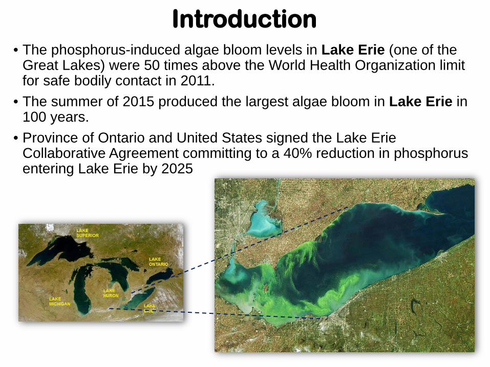
Introduction• The phosphorus-induced algae bloom levels in Lake Erie (one of the
Great Lakes) were 50 times above the World Health Organization limit for safe bodily contact in 2011.
• The summer of 2015 produced the largest algae bloom in Lake Erie in 100 years.
• Province of Ontario and United States signed the Lake Erie Collaborative Agreement committing to a 40% reduction in phosphorus entering Lake Erie by 2025

Introduction• Models in combination of monitoring can be used make better
management decisions to solve emerging phosphorus and water quality issues
• Watersheds (e.g. WLEB) contributes to Lake Erie from USA side was modeled using SWAT and is being used for various decision making
• In Ontario, Thames River basin and Grand River basin which are major contributors to Lake Erie are simulated individually with different models
• In addition several small scale watersheds are simulated in greater details
• GLASSI priority subwatersheds
• There is a need to simulate entire contributing basin to the Lake Erie from Ontarian side to understand the spatio-temporal differences
• Use the model to make better management decisions

Introduction• The accuracy of a model output is greatly dependent upon the
quality of the input data including their spatial and temporal resolution
• Inputs typically used in models are digital elevation models (DEMs), landuse and land management, soils and precipitation
• Input data available from difference sources and in different resolution
• Global – coarse resolution –Less HRUs – faster simulation time• E.g. FAO soils, GLCC landuse
• Local – finer resolution – higher HRU’s – Lower simulation time• E.g. SLC soils, SOLARIS landuse
• Need to critically analyze the data sources and resolution needed for large scale modeling in Ontario
• In USA, several studies performed input data analysis and have provided recommendation
Objectives
Overall goal is to evaluate the impacts of various data inputs on watershed hydrological processes and streamflow in Northern Lake Erie Basin
Objectives are• Prepare various inputs from different sources in SWAT format • Develop SWAT model for Northern Lake Erie Basin in Ontario
that contributes to Lake Erie• Investigate the impacts of landuse, soil and weather

Study AreaNorthern lake Erie Basin

Inputs
• DEM• 10m DEM
Inputs
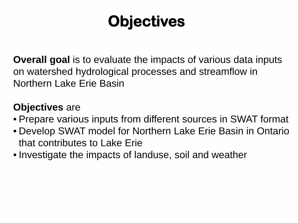
Landuse SWAT Area [ha] %Wat.Area
Barren BARR 5430 0.25Range-Grasses RNGE 14204 0.65Forest-Mixed FRST 36810 1.69Forest-Deciduous FRSD 119221 5.48Range-Brush RNGB 163039 7.5Water WATR 14931 0.69Agricultural Land-Row Crops AGRR 1290220 59.32Transportation UTRN 71886 3.31Residential-Med/Low URML 26209 1.2Residential-High Density URHD 67142 3.09Agricultural Land-Generic AGRL 365937 16.82
Agriculture: 76.14%
Landuse• SOLARIS (Southern Ontario Land Resource Information System)
• provides a comprehensive, standardized• Landscape level inventory of natural, rural and urban lands
• SOLARIS V2 used • 1:50,000 scale• Resolution: 30m

Inputs
Landuse SWAT Code Area [ha] %Wat.Ar
eaResidential-Medium Density URMD 30273.73 1.39Agricultural Land-Row Crops AGRR 2009463 92.39GRASSLAND GRAS 15314.33 0.7SHRUBLAND SHRB 16.5627 0SAVANNA SAVA 1649.973 0.08DECIDUOUS BROADLEAF FOREST FODB 79695.97 3.66EVERGREEN NEEDLELEAF FOREST FOEN 8242.396 0.38MIXED FOREST FOMI 22371.95 1.03Water WATR 7421.01 0.34WOODED TUNDRA TUWO 579.6061 0.03
Landuse• GLCC (Global Land Cover Characterization)• primarily unsupervised classification
• 10-day NDVI composites• Resolution: 1km
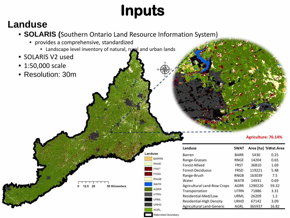
InputsSoils
SLC FAO
SLC: Soil Landscapes of Canada (SLC) version 3.2 • Contains soil map of Canada together with
major characteristics of soil for the whole country.
• Resolution of 1:1 million • Prepared by Agriculture and Agri-Food
Canada. • Each polygon on the map describes a
distinct type of soil and its associated characteristics.
FAO Soil (Global database of soils)• Joint FA0/Unesco Soil Map • Resolution 1: 5 million• MWSWAT has soils database in SWAT format

InputsWeather
• CFSR (Climate Forecast System Reanalysis): a global, high resolution, coupled atmosphere-ocean-land surface-sea ice system
• Provides the best estimate of the state of these coupled domains over this period• Resolution: 38 sq. km• 1979 to 2014
• GCDC (Gridded Climate Dataset for Canada): • Prepared by Agriculture and Agri-Food Canada (AAFC)• Resolution: 10 km gridded • Period of 1961-2003. • The data were interpolated from daily Environment Canada climate station observations
• using a thin plate smoothing spline surface fitting method implemented by ANUSPLIN V4.3.• Measured: climate stations

Methods• Developed SWAT models with combinations of inputs
• 10m DEM, SLC soil, SOLARIS landuse – Model 1• 10m DEM, SLC soil, GLCC landuse – Model 2• 10m DEM, FAO soil, SOLARIS landuse – Model 3• 10m DEM, FAO soil, GLCC landuse – Model 4
• Weather (measured, CFSR, GCDC) inputs added separately in each model • HRU delineation
• 0-2, 2-4,4-9999• Threshold: 5/5/5 – landuse/soil/slope
Model 1: 3831 Model 2: 1470 Model 3: 2961 Model 4: 1159 • Tile Drainage
• All agricultural lands in 0-2% slope (Daggupati et al., 2015)• Ddrain: 1000• Gdrain: 48• Tdrain:24• D_IMP: 2100• Daily curve number calculation method: Plant Based ET• CNCOEFF = 0.5
• Land management• Corn – Soybean rotation based on Heat units• Auto fertilization
• No calibration

MethodsVarious scenarios developed
Model 1• SC1: SLC soil, SOLARIS landuse, GCDC• SC2: SLC soil, SOLARIS landuse, CFSR• SC3: SLC soil, SOLARIS landuse, MeasuredModel 2• SC4: SLC soil, GLCC landuse, GCDC• SC5: SLC soil, GLCC landuse, CFSR• SC6: SLC soil, GLCC landuse, MeasuredModel 3• SC7: FAO soil, SOLARIS landuse, GCDC• SC8: FAO soil, SOLARIS landuse, CFSR• SC9: FAO soil, SOLARIS landuse, MeasuredModel 4• SC10: FAO soil, GLCC landuse, GCDC• SC11: FAO soil, GLCC landuse, CFSR• SC12: FAO soil, GLCC landuse, Measured

Methods
• Streamflow comparison stations
Thames at Ingresol
Thames at Thamesville
Bear creek at brigden
Grand at Brandford
Grand at Marsville
Bigcreek at Walsingham

ResultsHydrological budget
• Compare weather (GCDC vs. CFSR vs. Measured)
939
105 145 98
357
107
536
1129
170246
164
592
175
466
970
114 150101
373
110
551
0
200
400
600
800
1000
1200
PRECIP SURFACERUNOFF Q
TILE QGROUNDWATER (SHAL
AQ) Q
TOTAL WATERYLD
PERCOLATIONOUT OF SOIL
ET
Aver
age
Annu
al h
ydro
logy
(mm
)
SC1 SC2 SC3
• Compare landuse (Solaris vs GLCC)
SLC soil, GCDC weather FAO soil, GCDC weather
SLC soil, Solaris landuse

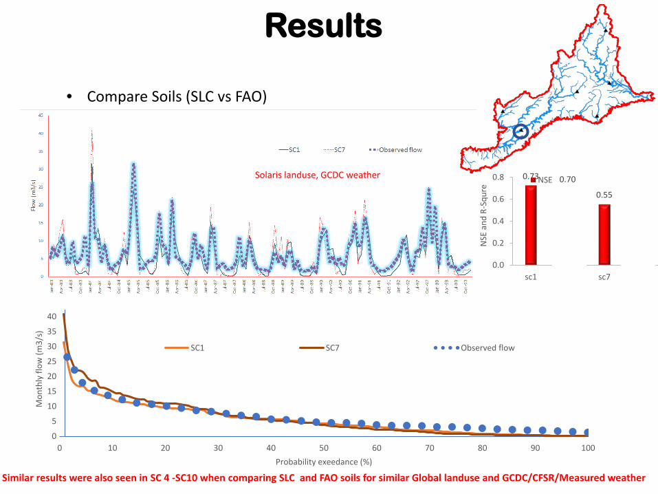
Results
• Compare Soils (SLC vs FAO)
SOLARIS landuse, GCDC weather GLCC landuse, GCDC weather
• Compare fine resolution vs coarse resolution datasets
939
105 145 98
357
107
536
1129
313 323
7
655
8
432
0
200
400
600
800
1000
1200
PRECIP SURFACERUNOFF Q
TILE Q GROUNDWATER(SHAL AQ) Q
TOTAL WATERYLD
PERCOLATIONOUT OF SOIL
ET
Aver
age
Annu
al h
ydro
logy
(mm
)
SC1 SC11
SLC soil SOLARIS landuse, GCDC weather VS FAO soil, GLCC landuse, CFSR weather
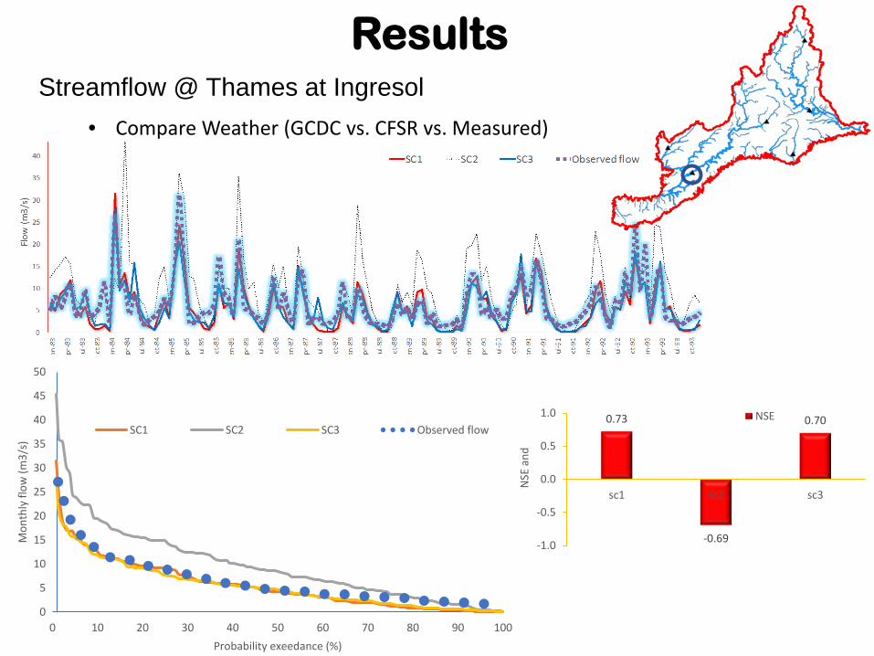
ResultsStreamflow @ Thames at Ingresol
• Compare Weather (GCDC vs. CFSR vs. Measured)
0
5
10
15
20
25
30
35
40
45
50
0 10 20 30 40 50 60 70 80 90 100
Mon
thly
flow
(m3/
s)
Probability exeedance (%)
SC1 SC2 SC3 Observed flow0.73
-0.69
0.70
-1.0
-0.5
0.0
0.5
1.0
sc1 sc2 sc3
NSE
and
NSE

Results
• Compare Landuse (Solaris vs GLCC)
SLC soil, GCDC weather 0.73 0.70
0.55
0.0
0.2
0.4
0.6
0.8
sc1 sc4 sc7
NSE
and
R-S
qure
NSE
05
10152025303540
0 10 20 30 40 50 60 70 80 90 100
Mon
thly
flow
(m3/
s)
Probability exeedance (%)
SC1 SC4 Observed flow
Similar results were also seen in Sc 7 and SC10 when comparing Solaris and Global landuse for similar FAO and GCDC/CFSR/Measured weather
0
5
10
15
20
25
30
35
40
45
0 10 20 30 40 50 60 70 80 90 100
Mon
thly
flow
(m3/
s)
Probability exeedance (%)
SC1 SC7 Observed flow
Results
• Compare Soils (SLC vs FAO)
Solaris landuse, GCDC weather 0.73 0.70
0.55
0.40
0.0
0.2
0.4
0.6
0.8
sc1 sc4 sc7 sc10
NSE
and
R-S
qure
NSE
Similar results were also seen in SC 4 -SC10 when comparing SLC and FAO soils for similar Global landuse and GCDC/CFSR/Measured weather

ResultsSimilar results in • Thames at Thamesville• Grand at Brantford• Grand at Marseville• Bear creek at Bridgton
• GCDC and Measured weather are similar • CFSR over estimated• Landuse (SOLARIS and Global) results looked similar• Soils (SLC vs FAO) results varied
• Observed and simulated differ significantly (next slide)• But the overall trends of weather, landuse, soil are similar
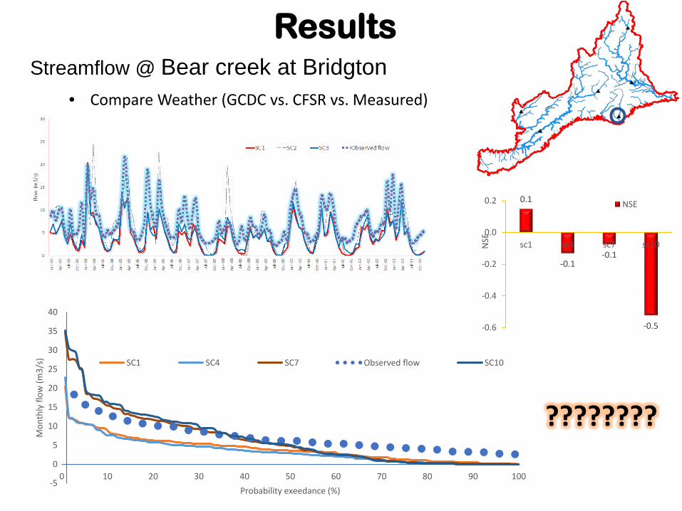
ResultsStreamflow @ Bear creek at Bridgton
• Compare Weather (GCDC vs. CFSR vs. Measured)
-5
0
5
10
15
20
25
30
35
40
0 10 20 30 40 50 60 70 80 90 100
Mon
thly
flow
(m3/
s)
Probability exeedance (%)
SC1 SC4 SC7 Observed flow SC10
0.1
-0.1-0.1
-0.5-0.6
-0.4
-0.2
0.0
0.2
sc1 sc4 sc7 sc10NSE
NSE
????????
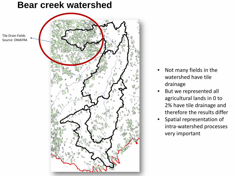
Tile Drain Fields Source: OMAFRA
Bear creek watershed
• Not many fields in the watershed have tile drainage
• But we represented all agricultural lands in 0 to 2% have tile drainage and therefore the results differ
• Spatial representation of intra-watershed processes very important
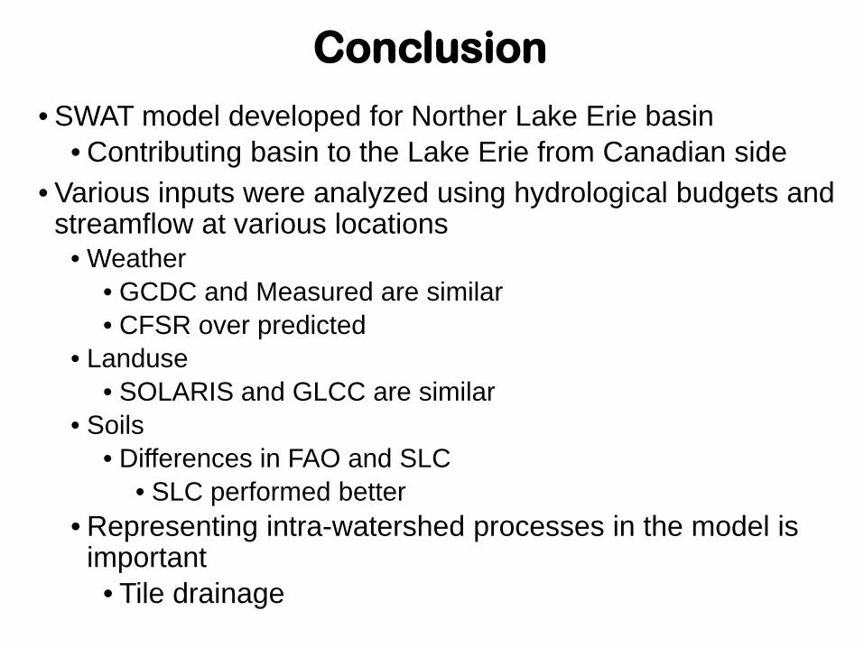
Conclusion
• SWAT model developed for Norther Lake Erie basin• Contributing basin to the Lake Erie from Canadian side
• Various inputs were analyzed using hydrological budgets and streamflow at various locations
• Weather• GCDC and Measured are similar• CFSR over predicted
• Landuse• SOLARIS and GLCC are similar
• Soils• Differences in FAO and SLC
• SLC performed better• Representing intra-watershed processes in the model is
important• Tile drainage
Thanks


