N ik o l a o s Lio n is
U n i v e r s i t y O f A t h e n s
( R e v i s e d : O c t o b e r 2 0 1 4 )
Introduction to Game Theory 1
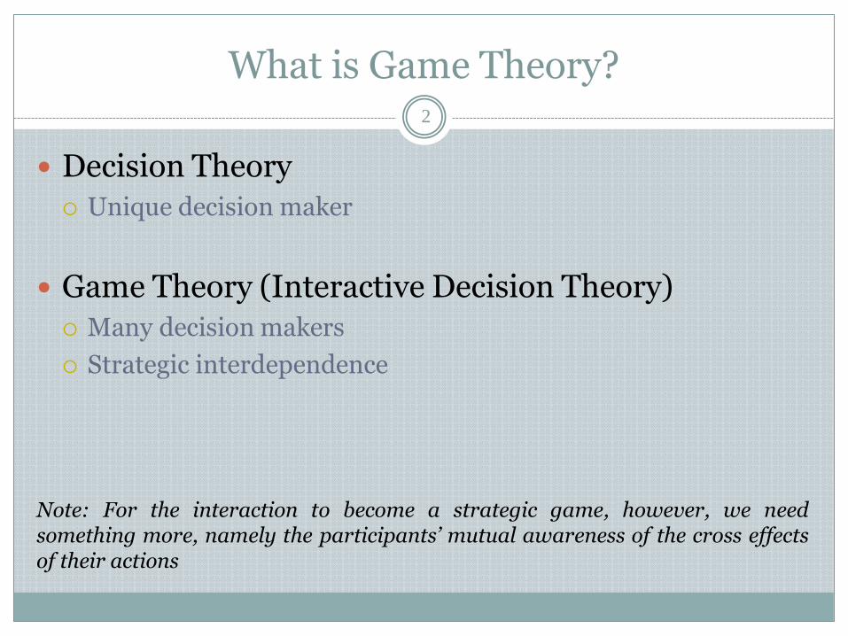
What is Game Theory?
Decision Theory Unique decision maker
Game Theory (Interactive Decision Theory) Many decision makers
Strategic interdependence
Note: For the interaction to become a strategic game, however, we need something more, namely the participants’ mutual awareness of the cross effects of their actions
2
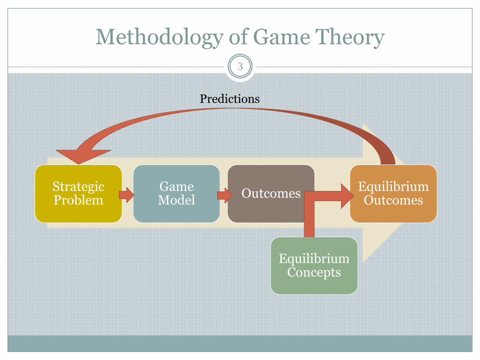
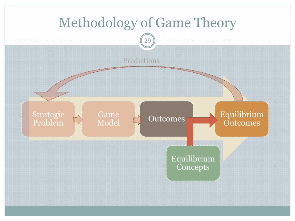
Methodology of Game Theory 3
Strategic Problem
Game Model
Outcomes
Equilibrium Concepts
Equilibrium Outcomes
Predictions
F R O M A S T R A T E G I C P R O B L E M
T O A G A M E M O D E L
4
Constructing a Game
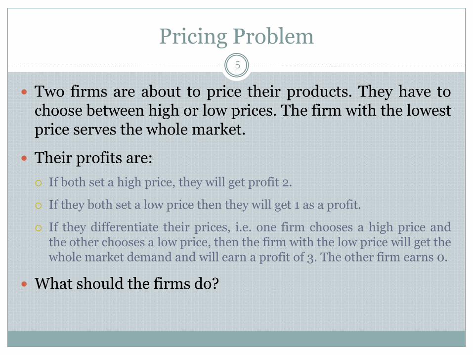
Pricing Problem 5
Two firms are about to price their products. They have to choose between high or low prices. The firm with the lowest price serves the whole market.
Their profits are:
If both set a high price, they will get profit 2.
If they both set a low price then they will get 1 as a profit.
If they differentiate their prices, i.e. one firm chooses a high price and the other chooses a low price, then the firm with the low price will get the whole market demand and will earn a profit of 3. The other firm earns 0.
What should the firms do?
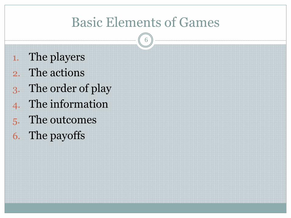
Basic Elements of Games 6
1. The players
2. The actions
3. The order of play
4. The information
5. The outcomes
6. The payoffs
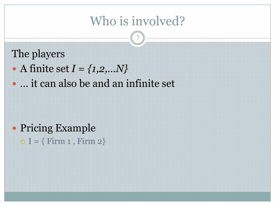
Who is involved? 7
The players
A finite set I = {1,2,…N}
… it can also be and an infinite set
Pricing Example I = { Firm 1 , Firm 2}
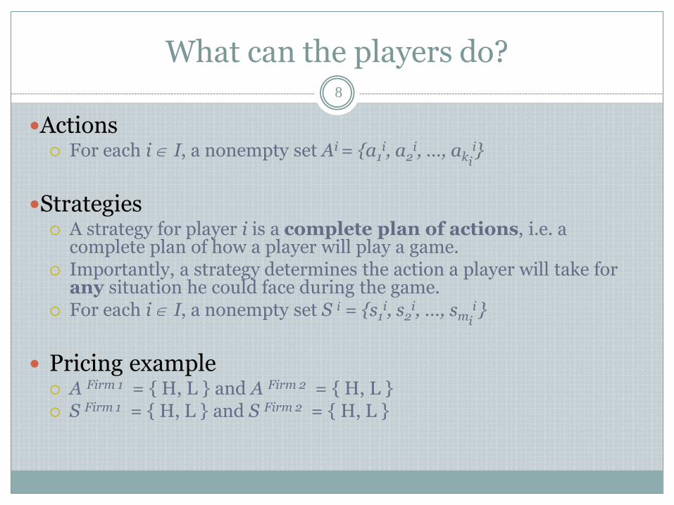
What can the players do?
Actions For each i I, a nonempty set Ai = {a1
i, a2i, …, aki
i}
Strategies
A strategy for player i is a complete plan of actions, i.e. a complete plan of how a player will play a game.
Importantly, a strategy determines the action a player will take for any situation he could face during the game.
For each i I, a nonempty set S i = {s1i, s2
i, …, smii }
Pricing example
A Firm 1 = { H, L } and A Firm 2 = { H, L } S Firm 1 = { H, L } and S Firm 2 = { H, L }
8
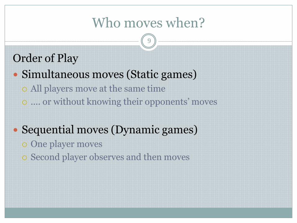
Who moves when?
Order of Play
Simultaneous moves (Static games) All players move at the same time
…. or without knowing their opponents’ moves
Sequential moves (Dynamic games) One player moves
Second player observes and then moves
9
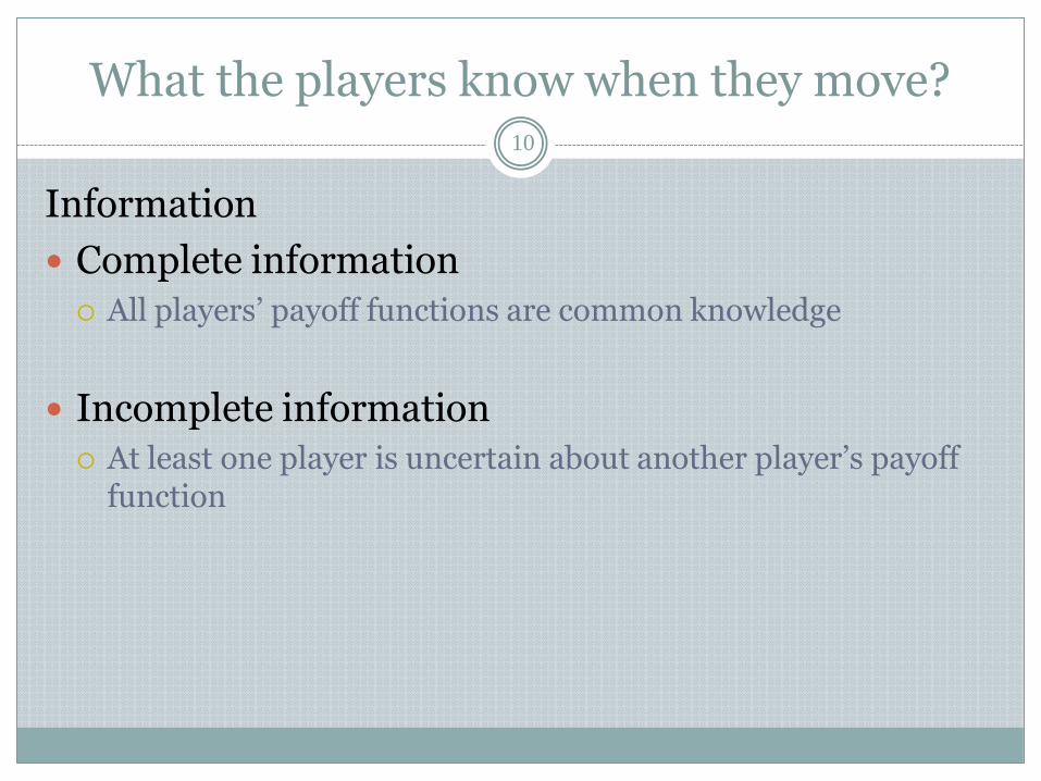
What the players know when they move?
Information
Complete information All players’ payoff functions are common knowledge
Incomplete information At least one player is uncertain about another player’s payoff
function
10
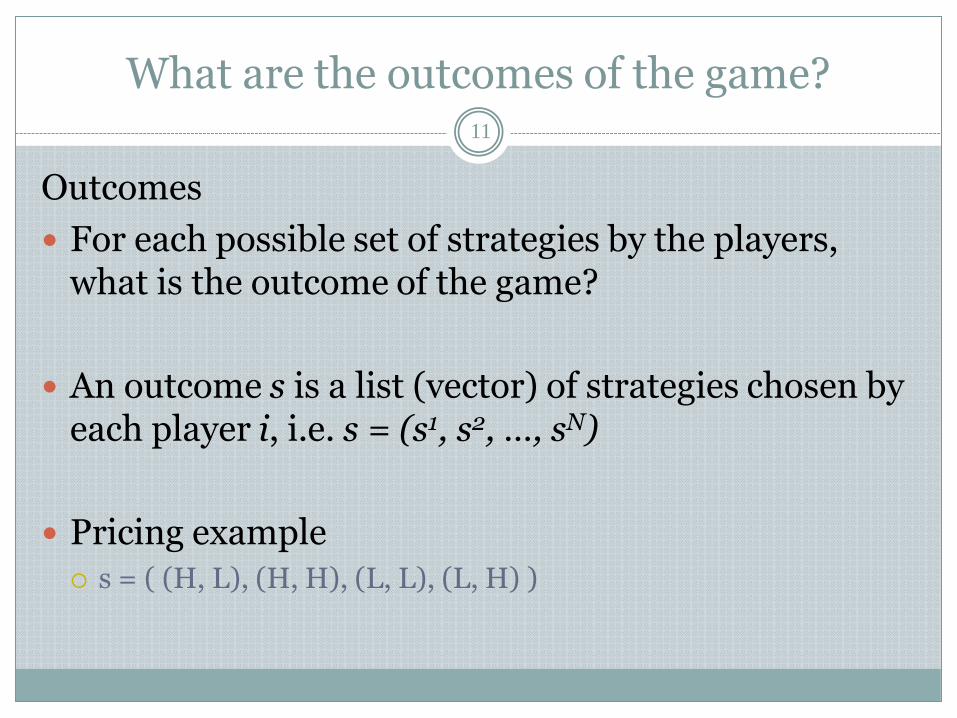
What are the outcomes of the game?
Outcomes
For each possible set of strategies by the players, what is the outcome of the game?
An outcome s is a list (vector) of strategies chosen by each player i, i.e. s = (s1, s2, …, sN)
Pricing example s = ( (H, L), (H, H), (L, L), (L, H) )
11
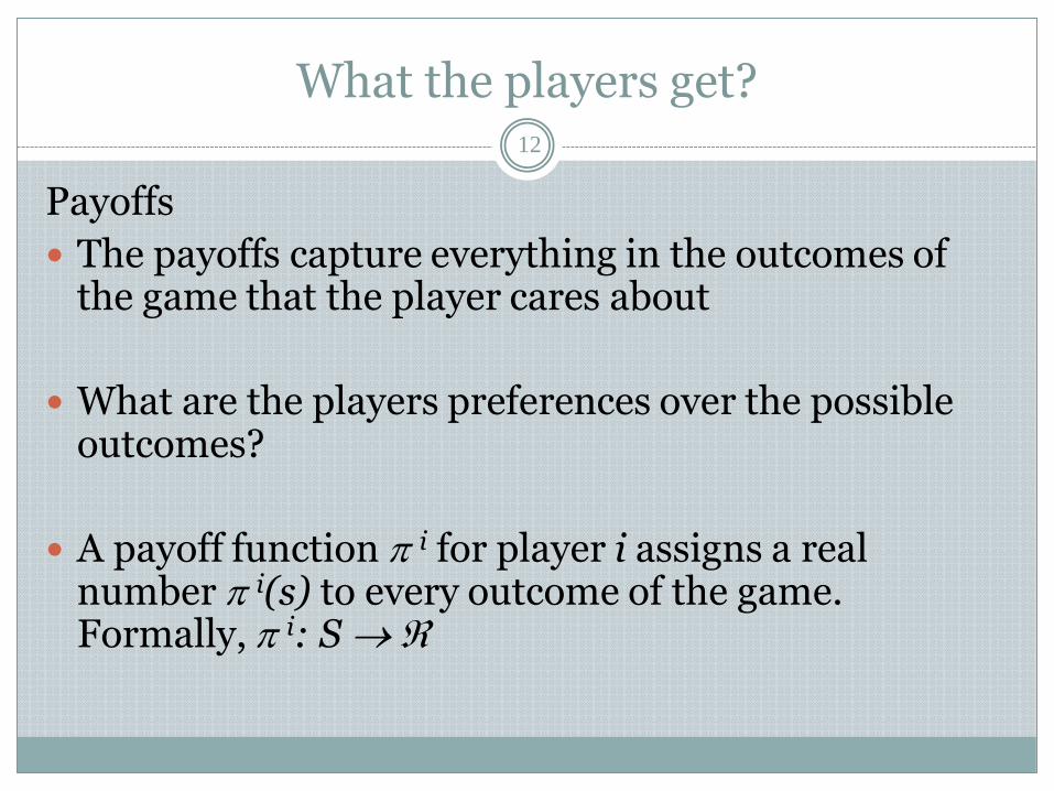
What the players get?
Payoffs
The payoffs capture everything in the outcomes of the game that the player cares about
What are the players preferences over the possible outcomes?
A payoff function i for player i assigns a real number i(s) to every outcome of the game. Formally, i: S
12
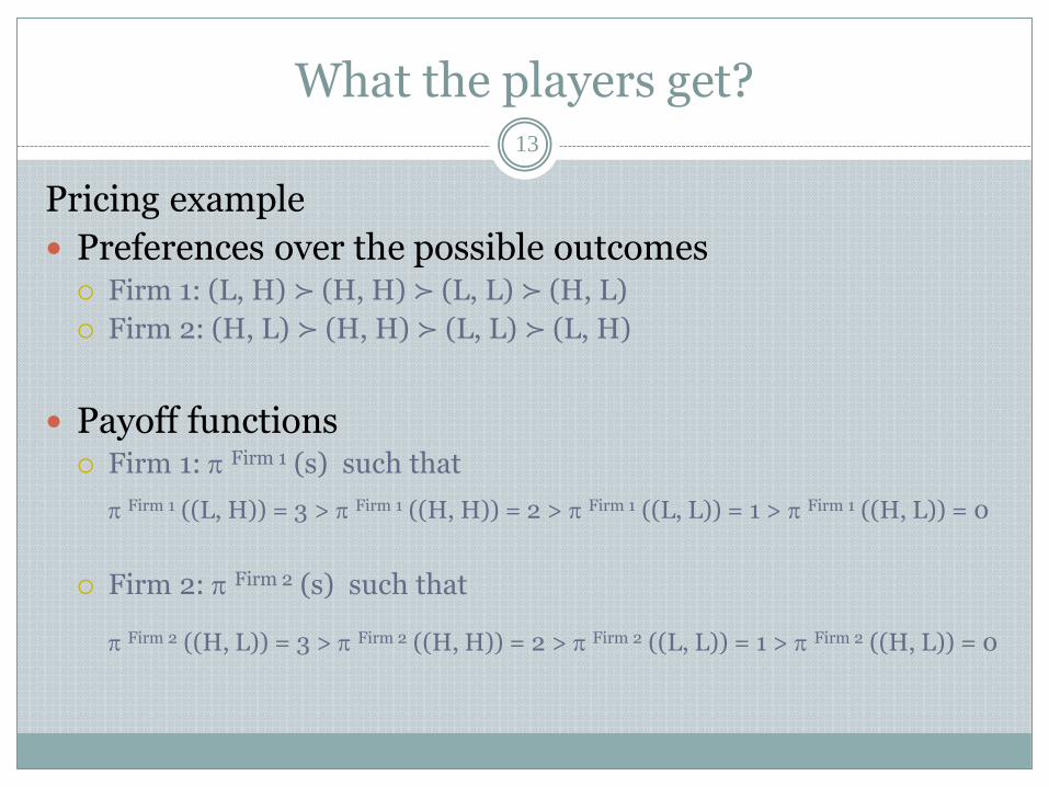
What the players get?
Pricing example
Preferences over the possible outcomes Firm 1: (L, H) ≻ (H, H) ≻ (L, L) ≻ (H, L)
Firm 2: (H, L) ≻ (H, H) ≻ (L, L) ≻ (L, H)
Payoff functions Firm 1: Firm 1 (s) such that
Firm 1 ((L, H)) = 3 > Firm 1 ((H, H)) = 2 > Firm 1 ((L, L)) = 1 > Firm 1 ((H, L)) = 0
Firm 2: Firm 2 (s) such that
Firm 2 ((H, L)) = 3 > Firm 2 ((H, H)) = 2 > Firm 2 ((L, L)) = 1 > Firm 2 ((H, L)) = 0
13
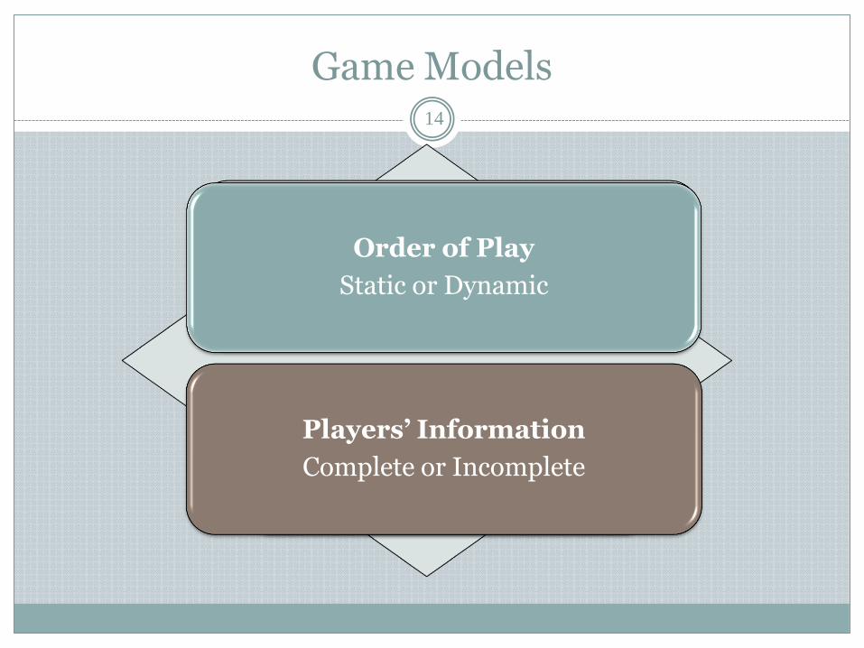
Game Models 14
Order of Play
Static or Dynamic
Players’ Information
Complete or Incomplete
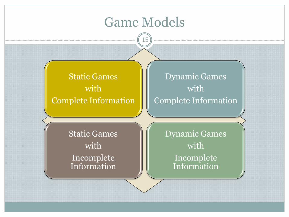
Game Models 15
Static Games
with
Complete Information
Dynamic Games
with
Complete Information
Static Games
with
Incomplete Information
Dynamic Games
with
Incomplete Information
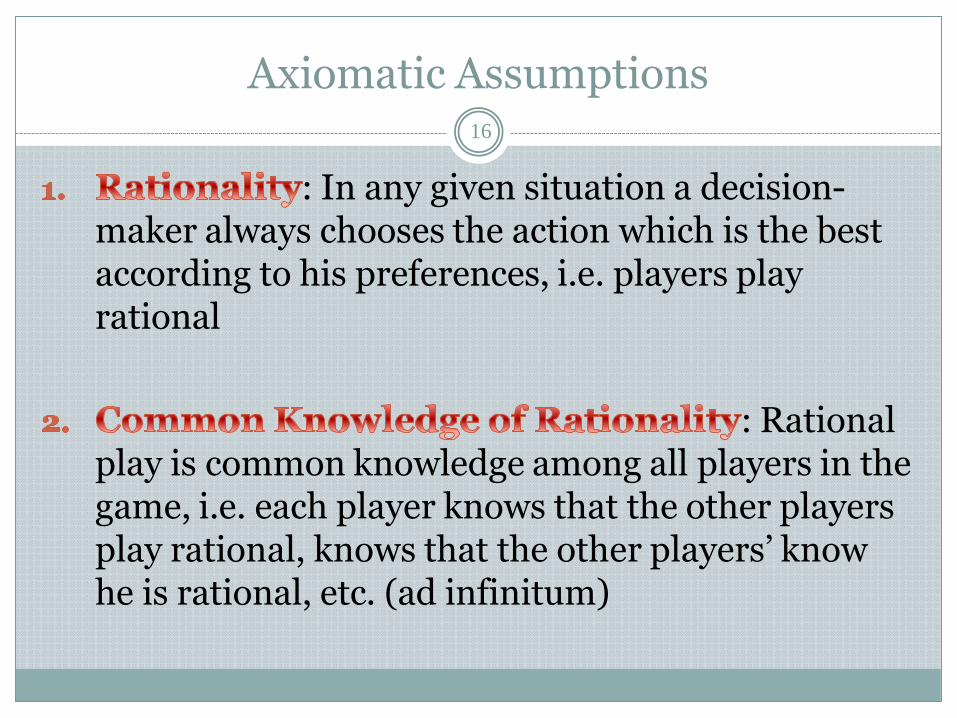
Axiomatic Assumptions 16
: In any given situation a decision-maker always chooses the action which is the best according to his preferences, i.e. players play rational
: Rational play is common knowledge among all players in the game, i.e. each player knows that the other players play rational, knows that the other players’ know he is rational, etc. (ad infinitum)
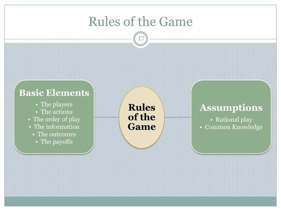
Rules of the Game 17
Rules of the Game
Basic Elements • The players • The actions
• The order of play • The information
• The outcomes • The payoffs
Assumptions • Rational play
• Common Knowledge
N O R M A L F O R M
A N D
E X T E N S I V E F O R M
18
Representations of Games
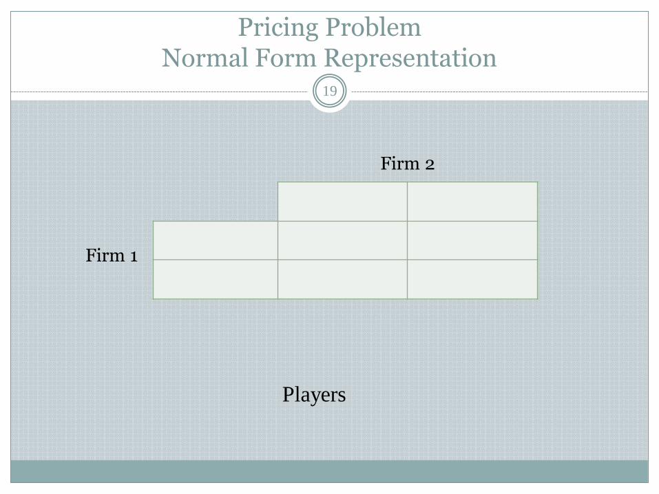
Pricing Problem Normal Form Representation
19
Firm 2
Firm 1
Players
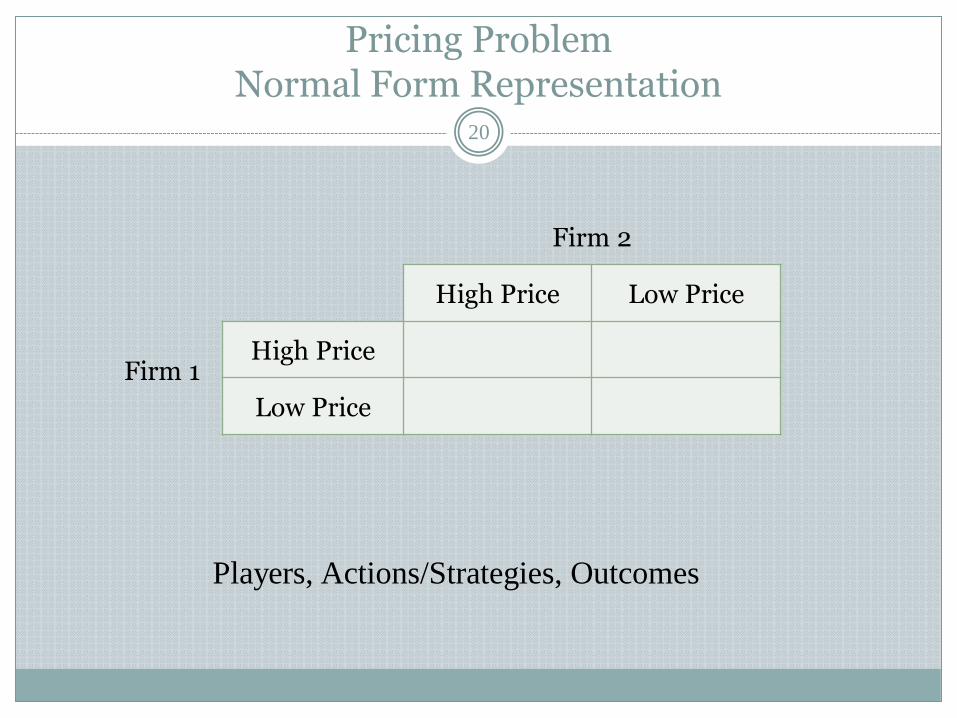
Pricing Problem Normal Form Representation
20
Firm 2
High Price Low Price
Firm 1
High Price
Low Price
Players, Actions/Strategies, Outcomes
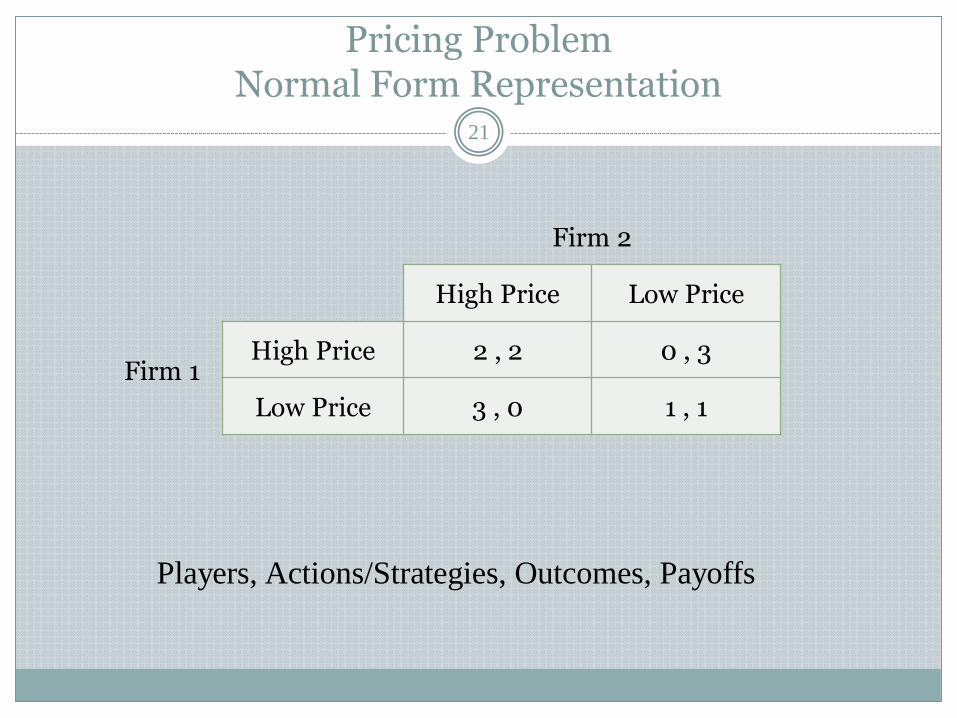
Pricing Problem Normal Form Representation
21
Firm 2
High Price Low Price
Firm 1
High Price 2 , 2 0 , 3
Low Price 3 , 0 1 , 1
Players, Actions/Strategies, Outcomes, Payoffs
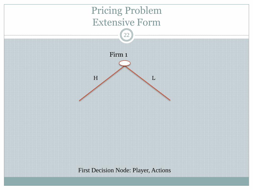
Pricing Problem Extensive Form
22
Firm 1
L H
First Decision Node: Player, Actions
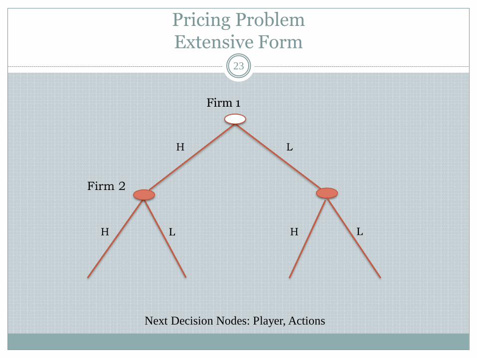
Pricing Problem Extensive Form
23
Firm 1
Firm 2
L H L H
L H
Next Decision Nodes: Player, Actions
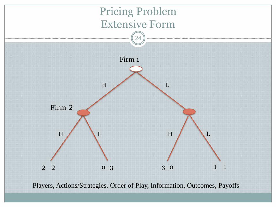
Pricing Problem Extensive Form
24
Firm 1
Firm 2
L H L H
L H
2 2 0 3 3 0 1 1
Players, Actions/Strategies, Order of Play, Information, Outcomes, Payoffs
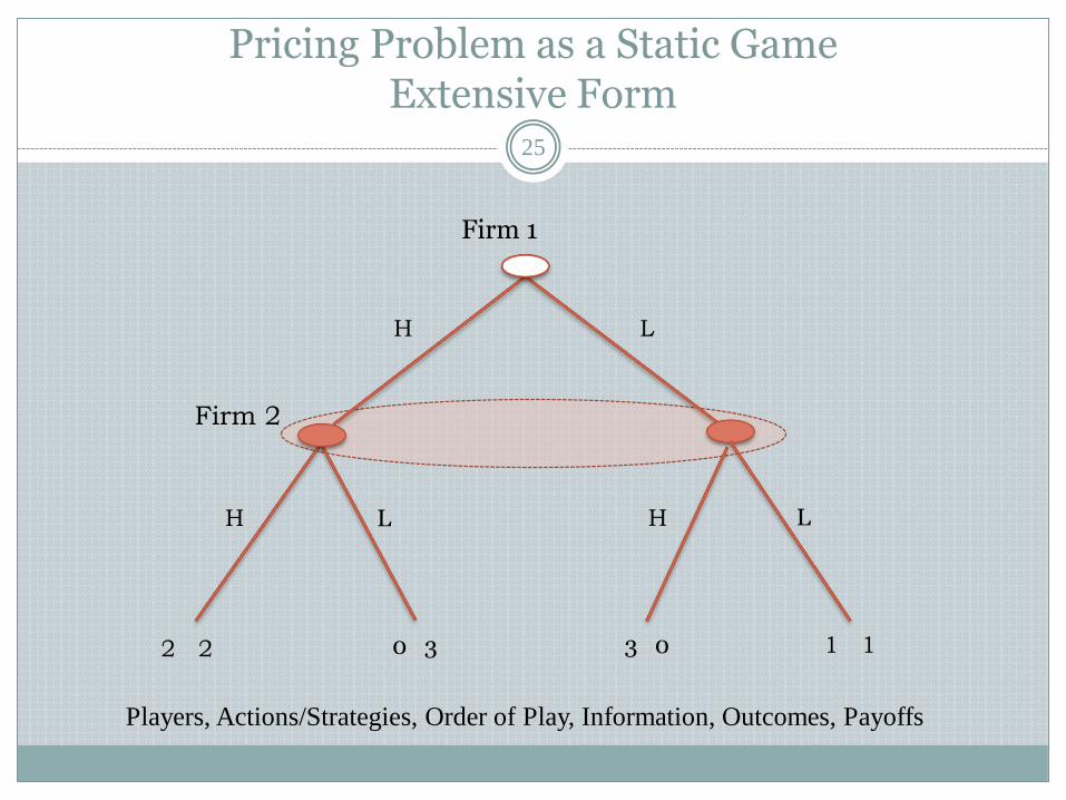
Pricing Problem as a Static Game Extensive Form
25
Firm 1
Firm 2
L H L H
L H
2 2 0 3 3 0 1 1
Players, Actions/Strategies, Order of Play, Information, Outcomes, Payoffs
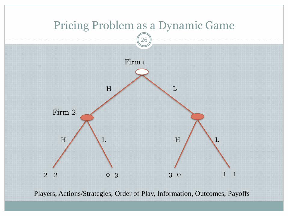
Pricing Problem as a Dynamic Game 26
Firm 1
Firm 2
L H L H
L H
2 2 0 3 3 0 1 1
Players, Actions/Strategies, Order of Play, Information, Outcomes, Payoffs
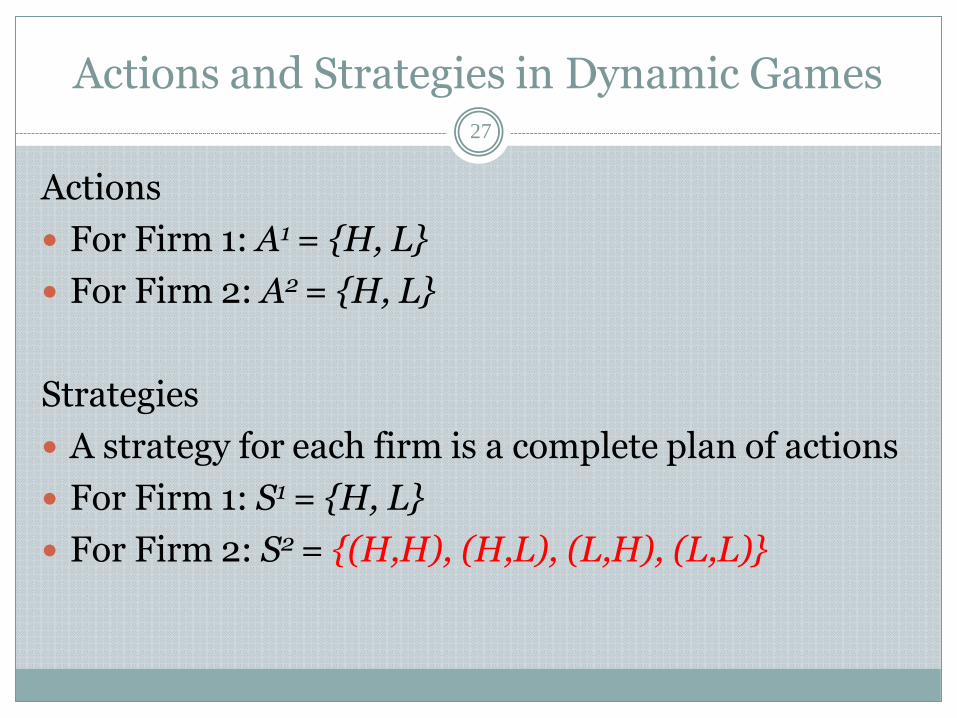
Actions and Strategies in Dynamic Games
Actions
For Firm 1: A1 = {H, L}
For Firm 2: A2 = {H, L}
Strategies
A strategy for each firm is a complete plan of actions
For Firm 1: S1 = {H, L}
For Firm 2: S2 = {(H,H), (H,L), (L,H), (L,L)}
27
F R O M O U T C O M E S
T O E Q U I L I B R I U M O U T C O M E S
28
Solving a Game
Methodology of Game Theory 29
Strategic Problem
Game Model
Outcomes
Equilibrium Concepts
Equilibrium Outcomes
Predictions
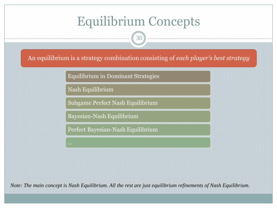
Equilibrium Concepts
An equilibrium is a strategy combination consisting of each player’s best strategy
Equilibrium in Dominant Strategies
Nash Equilibrium
Subgame Perfect Nash Equilibrium
Bayesian-Nash Equilibrium
Perfect Bayesian-Nash Equilibrium
…
30
Note: The main concept is Nash Equilibrium. All the rest are just equilibrium refinements of Nash Equilibrium.
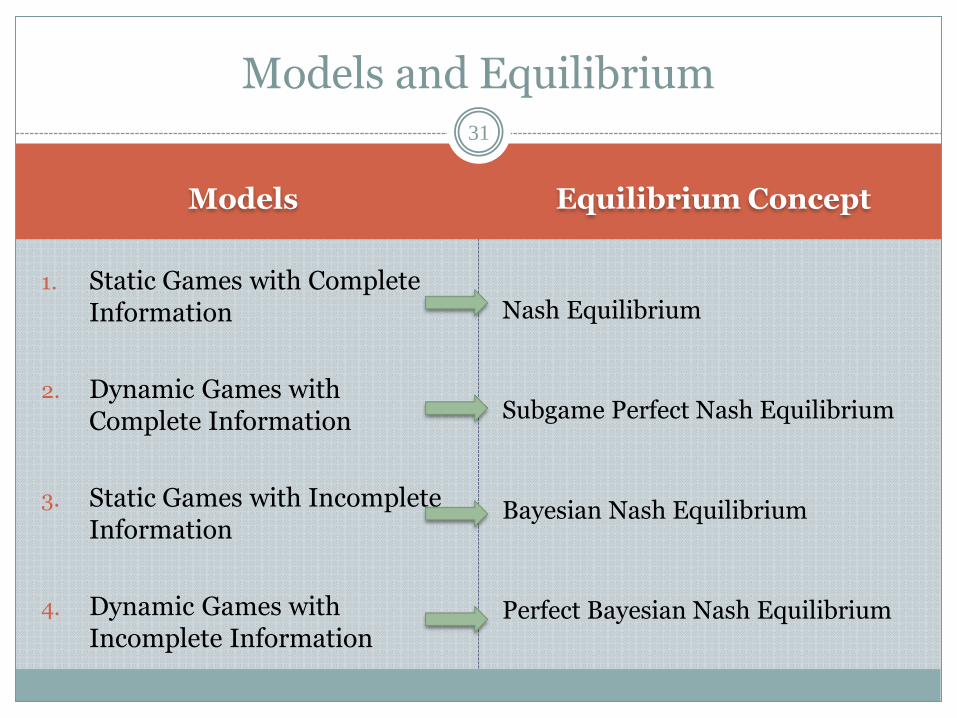
Models Equilibrium Concept
1. Static Games with Complete Information
2. Dynamic Games with Complete Information
3. Static Games with Incomplete Information
4. Dynamic Games with Incomplete Information
Nash Equilibrium
Subgame Perfect Nash Equilibrium
Bayesian Nash Equilibrium
Perfect Bayesian Nash Equilibrium
31
Models and Equilibrium
S T A T I C G A M E S
W I T H
C O M P L E T E I N F O R M A T I O N
A N D
N A S H E Q U I L I B R I U M
32
Solving a Static Game
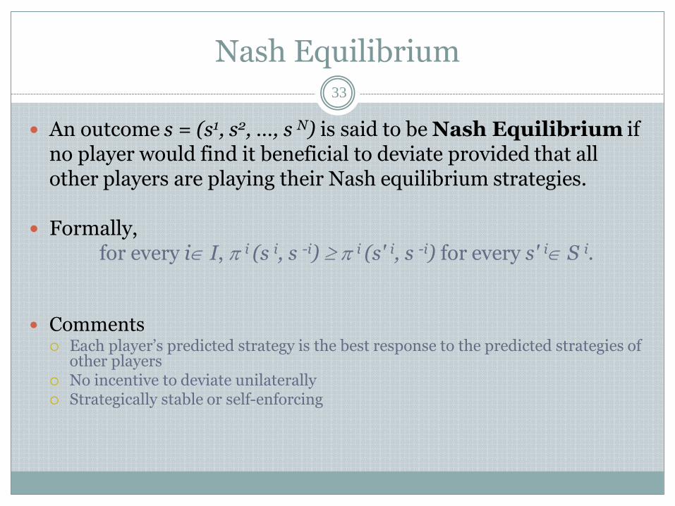
Nash Equilibrium
An outcome s = (s1, s2, …, s N) is said to be Nash Equilibrium if no player would find it beneficial to deviate provided that all other players are playing their Nash equilibrium strategies.
Formally,
for every i I, i (s i, s -i) i (s' i, s -i) for every s' i S i.
Comments Each player’s predicted strategy is the best response to the predicted strategies of
other players No incentive to deviate unilaterally Strategically stable or self-enforcing
33
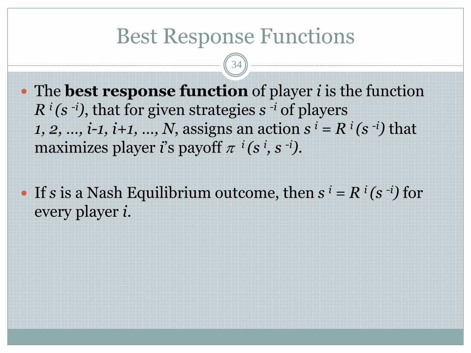
Best Response Functions
The best response function of player i is the function R i (s -i), that for given strategies s -i of players 1, 2, …, i-1, i+1, …, N, assigns an action s i = R i (s -i) that maximizes player i’s payoff i (s i, s -i).
If s is a Nash Equilibrium outcome, then s i = R i (s -i) for every player i.
34
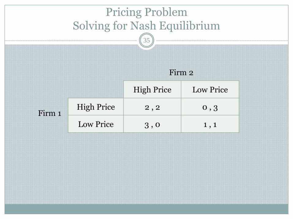
Pricing Problem Solving for Nash Equilibrium
35
Firm 2
High Price Low Price
Firm 1
High Price 2 , 2 0 , 3
Low Price 3 , 0 1 , 1
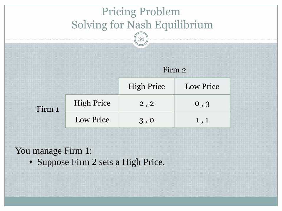
Pricing Problem Solving for Nash Equilibrium
36
Firm 2
High Price Low Price
Firm 1
High Price 2 , 2 0 , 3
Low Price 3 , 0 1 , 1
You manage Firm 1:
• Suppose Firm 2 sets a High Price.
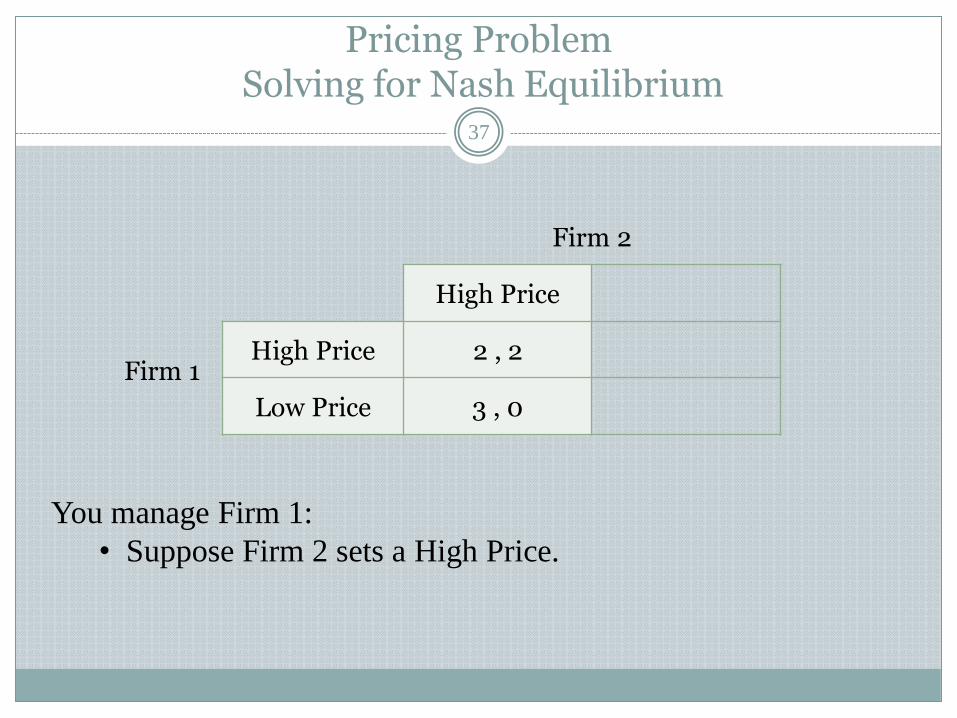
Pricing Problem Solving for Nash Equilibrium
37
Firm 2
High Price
Firm 1
High Price 2 , 2
Low Price 3 , 0
You manage Firm 1:
• Suppose Firm 2 sets a High Price.
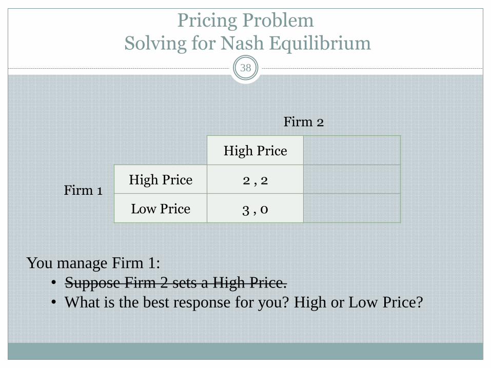
Pricing Problem Solving for Nash Equilibrium
38
Firm 2
High Price
Firm 1
High Price 2 , 2
Low Price 3 , 0
You manage Firm 1:
• Suppose Firm 2 sets a High Price.
• What is the best response for you? High or Low Price?
Pricing Problem Solving for Nash Equilibrium
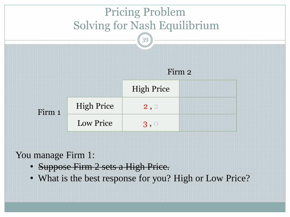
39
Firm 2
High Price
Firm 1
High Price 2 , 2
Low Price 3 , 0
You manage Firm 1:
• Suppose Firm 2 sets a High Price.
• What is the best response for you? High or Low Price?
Pricing Problem Solving for Nash Equilibrium
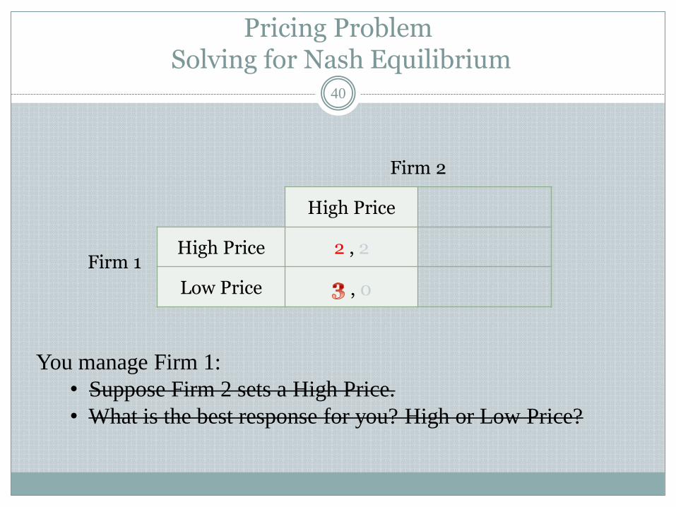
40
Firm 2
High Price
Firm 1
High Price 2 , 2
Low Price , 0
You manage Firm 1:
• Suppose Firm 2 sets a High Price.
• What is the best response for you? High or Low Price?
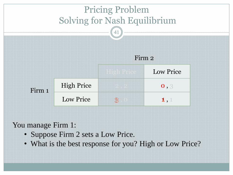
Pricing Problem Solving for Nash Equilibrium
41
Firm 2
High Price Low Price
Firm 1
High Price 2 , 2 0 , 3
Low Price , 0 , 1
You manage Firm 1:
• Suppose Firm 2 sets a Low Price.
• What is the best response for you? High or Low Price?
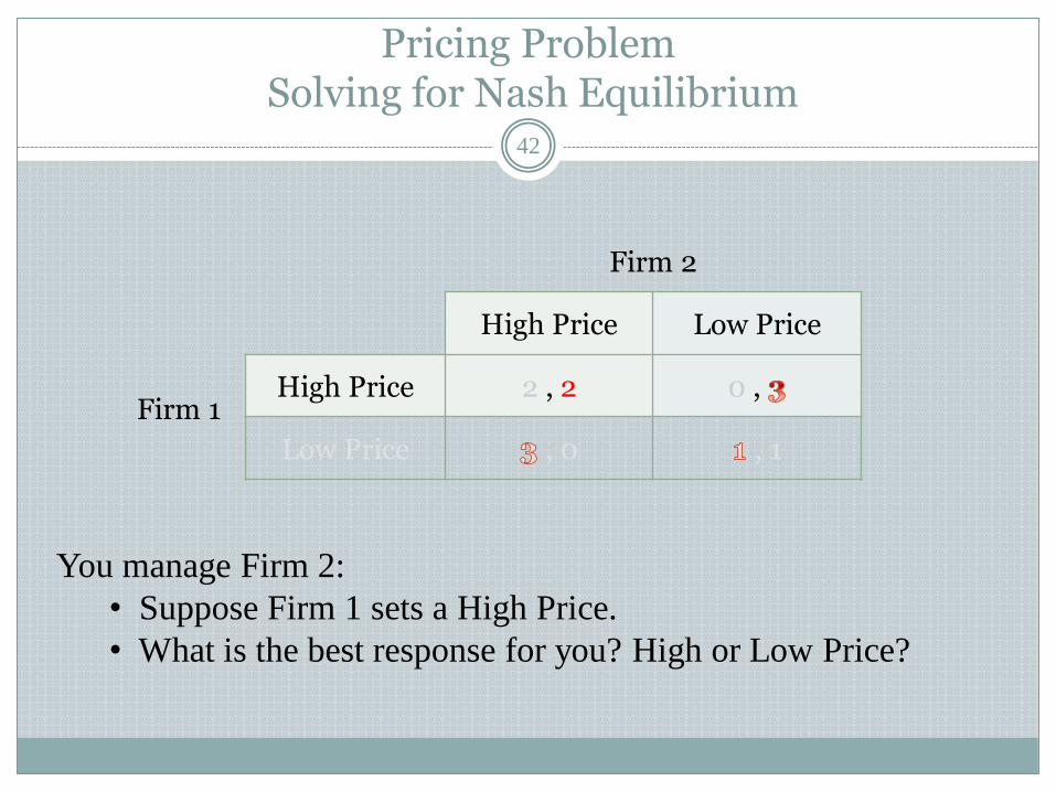
Pricing Problem Solving for Nash Equilibrium
42
Firm 2
High Price Low Price
Firm 1
High Price 2 , 2 0 ,
Low Price , 0 , 1
You manage Firm 2:
• Suppose Firm 1 sets a High Price.
• What is the best response for you? High or Low Price?
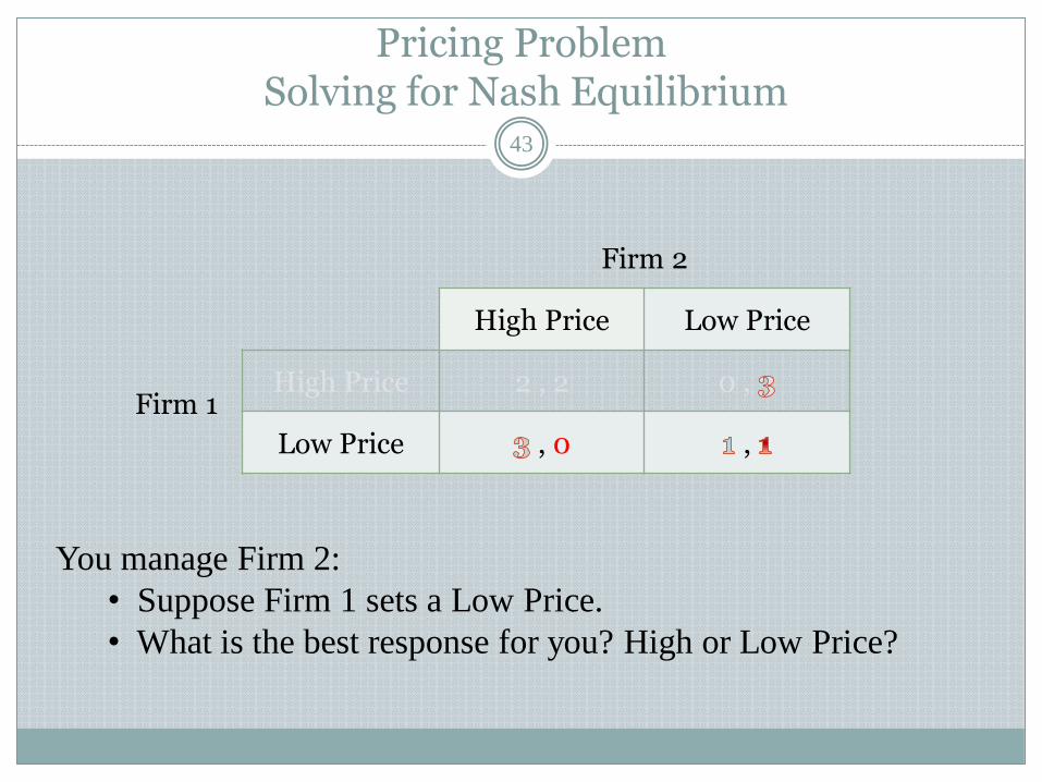
Pricing Problem Solving for Nash Equilibrium
43
Firm 2
High Price Low Price
Firm 1
High Price 2 , 2 0 ,
Low Price , 0 ,
You manage Firm 2:
• Suppose Firm 1 sets a Low Price.
• What is the best response for you? High or Low Price?
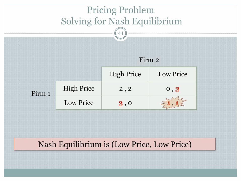
Pricing Problem Solving for Nash Equilibrium
44
Firm 2
High Price Low Price
Firm 1
High Price 2 , 2 0 ,
Low Price , 0 ,
Nash Equilibrium is (Low Price, Low Price)
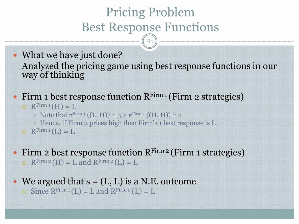
Pricing Problem Best Response Functions
What we have just done? Analyzed the pricing game using best response functions in our
way of thinking
Firm 1 best response function RFirm 1 (Firm 2 strategies) RFirm 1 (H) = L
Note that Firm 1 ((L, H)) = 3 > Firm 1 ((H, H)) = 2 Hence, if Firm 2 prices high then Firm’s 1 best response is L
RFirm 1 (L) = L
Firm 2 best response function RFirm 2 (Firm 1 strategies)
RFirm 2 (H) = L and RFirm 2 (L) = L
We argued that s = (L, L) is a N.E. outcome Since RFirm 1 (L) = L and RFirm 2 (L) = L
45
D Y N A M I C G A M E S
W I T H
C O M P L E T E I N F O R M A T I O N
A N D
S U B G A M E P E R F E C T N A S H E Q U I L I B R I U M
46
Solving a Dynamic Game
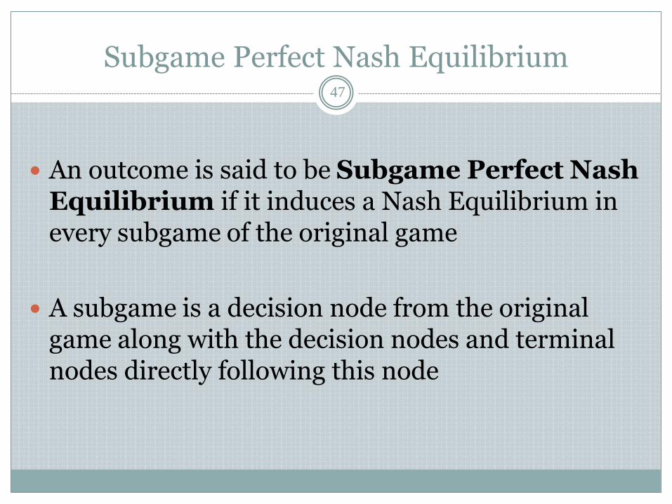
Subgame Perfect Nash Equilibrium
An outcome is said to be Subgame Perfect Nash Equilibrium if it induces a Nash Equilibrium in every subgame of the original game
A subgame is a decision node from the original game along with the decision nodes and terminal nodes directly following this node
47
Subgame 3
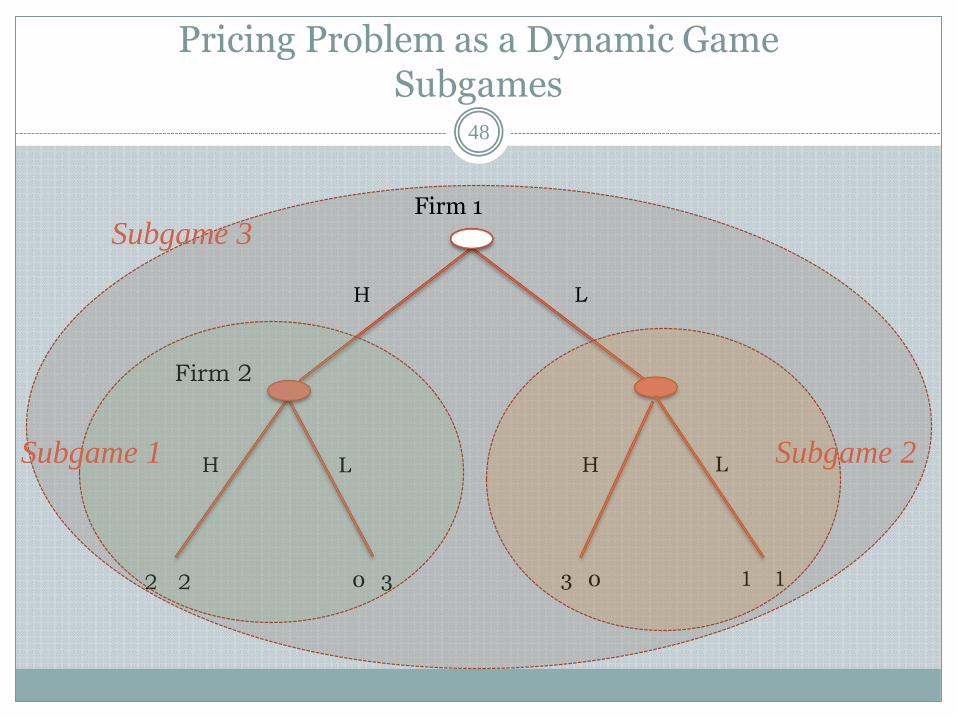
Pricing Problem as a Dynamic Game Subgames
48
Firm 1
Firm 2
L H L H
L H
2 2 0 3 3 0 1 1
Subgame 1 Subgame 2
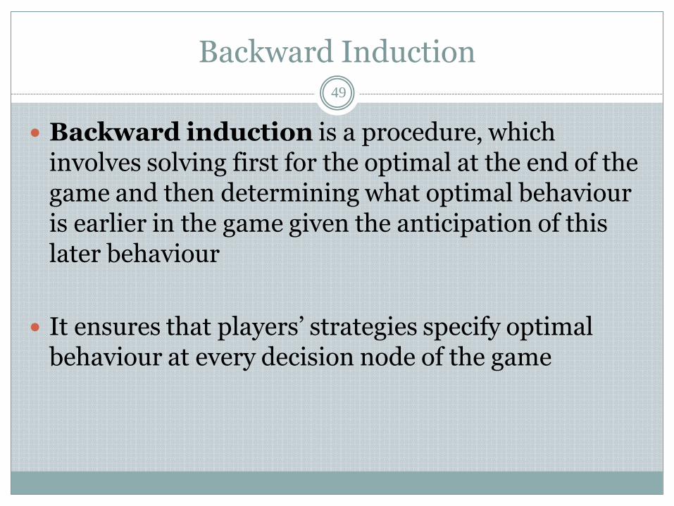
Backward Induction 49
Backward induction is a procedure, which involves solving first for the optimal at the end of the game and then determining what optimal behaviour is earlier in the game given the anticipation of this later behaviour
It ensures that players’ strategies specify optimal behaviour at every decision node of the game
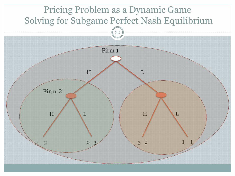
Pricing Problem as a Dynamic Game Solving for Subgame Perfect Nash Equilibrium
50
Firm 1
Firm 2
L H L H
L H
2 2 0 3 3 0 1 1
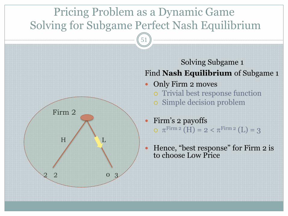
Pricing Problem as a Dynamic Game Solving for Subgame Perfect Nash Equilibrium
51
Firm 2
L H
2 2 0 3
Solving Subgame 1
Find Nash Equilibrium of Subgame 1
Only Firm 2 moves Trivial best response function Simple decision problem
Firm’s 2 payoffs Firm 2 (Η) = 2 < Firm 2 (L) = 3
Hence, “best response” for Firm 2 is to choose Low Price
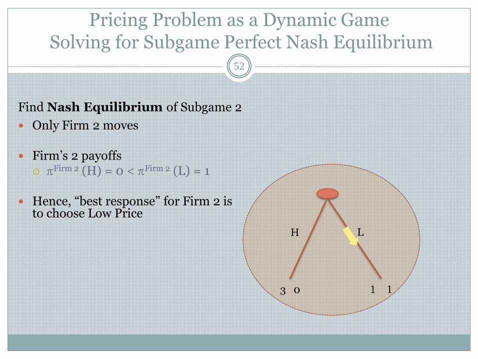
Pricing Problem as a Dynamic Game Solving for Subgame Perfect Nash Equilibrium
52
L H
3 0 1 1
Find Nash Equilibrium of Subgame 2
Only Firm 2 moves
Firm’s 2 payoffs Firm 2 (Η) = 0 < Firm 2 (L) = 1
Hence, “best response” for Firm 2 is to choose Low Price
Pricing Problem as a Dynamic Game Solving for Subgame Perfect Nash Equilibrium
53
Firm 1
Firm 2
L H L H
L H
2 2 0 3 3 0 1 1
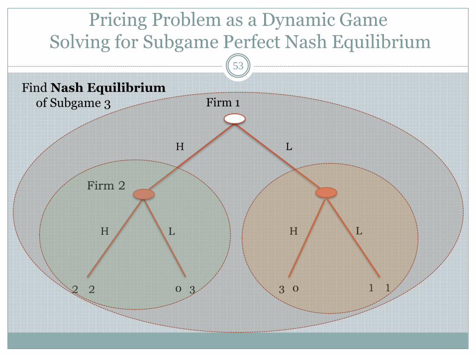
Find Nash Equilibrium of Subgame 3
Firm 1
L H
Pricing Problem as a Dynamic Game Solving for Subgame Perfect Nash Equilibrium
54
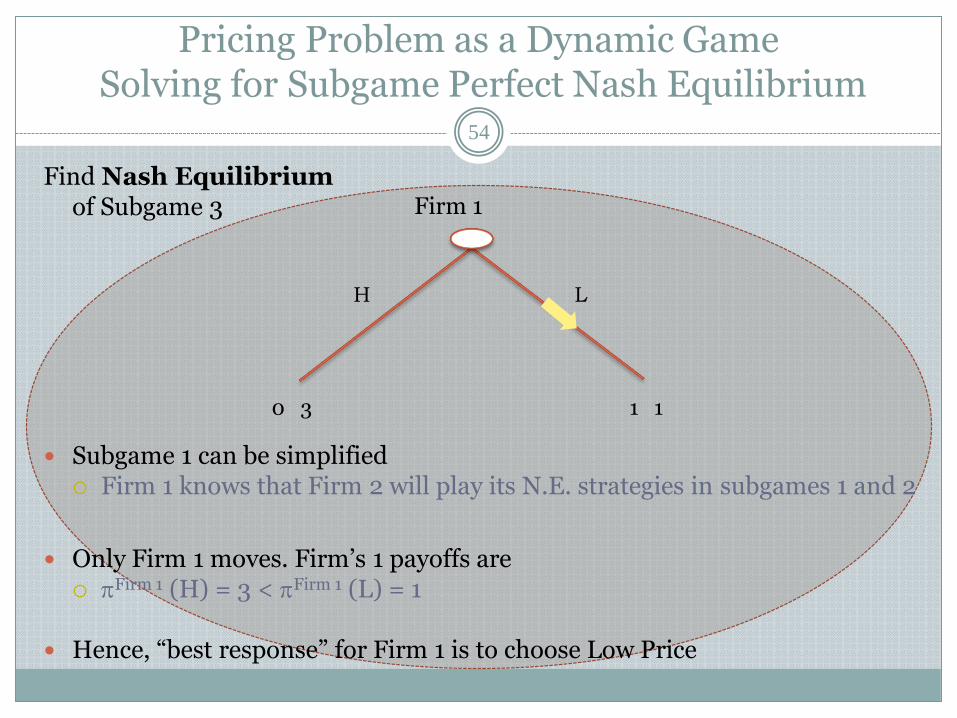
0 3 1 1
Subgame 1 can be simplified Firm 1 knows that Firm 2 will play its N.E. strategies in subgames 1 and 2
Only Firm 1 moves. Firm’s 1 payoffs are Firm 1 (Η) = 3 < Firm 1 (L) = 1
Hence, “best response” for Firm 1 is to choose Low Price
Find Nash Equilibrium of Subgame 3

Pricing Problem as a Dynamic Game Solving for Subgame Perfect Nash Equilibrium
55
Firm 1
Firm 2
L H L H
L H
2 2 0 3 3 0 1 1
Nash Equilibria of all the subagmes consitutes the Subgame Perfect Nash Equilibrium
The Subgame Perfect Nash Equilibrium is … not !!!
56
EXAMPLES
C O L L E C T I V E C H O I C E P R O B L E M
C O O R D I N A T I O N F A I L U R E
57
Prisoner’s Dilemma
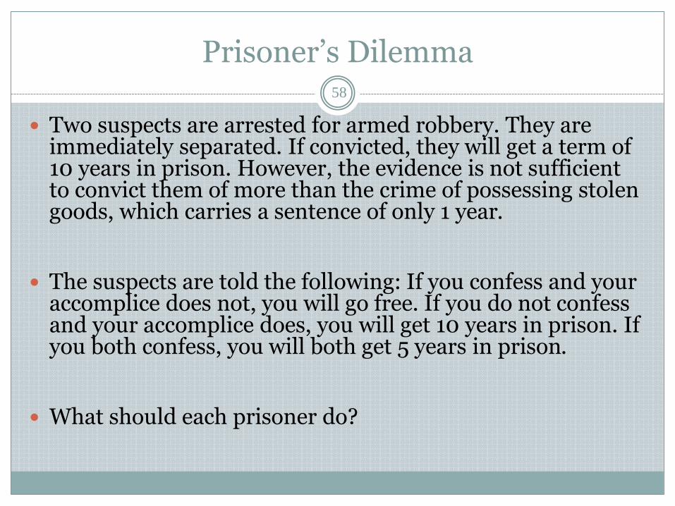
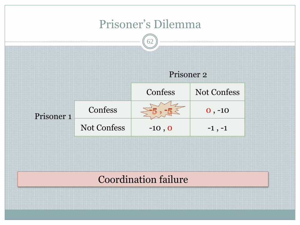
Prisoner’s Dilemma 58
Two suspects are arrested for armed robbery. They are immediately separated. If convicted, they will get a term of 10 years in prison. However, the evidence is not sufficient to convict them of more than the crime of possessing stolen goods, which carries a sentence of only 1 year.
The suspects are told the following: If you confess and your accomplice does not, you will go free. If you do not confess and your accomplice does, you will get 10 years in prison. If you both confess, you will both get 5 years in prison.
What should each prisoner do?
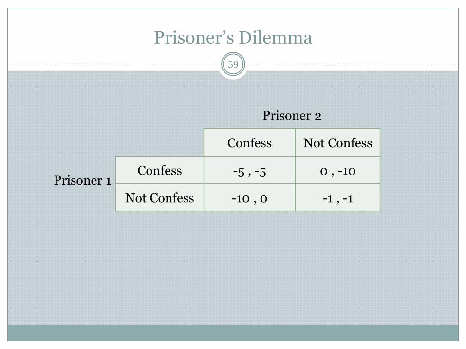
Prisoner’s Dilemma
59
Prisoner 2
Confess Not Confess
Prisoner 1
Confess -5 , -5 0 , -10
Not Confess -10 , 0 -1 , -1
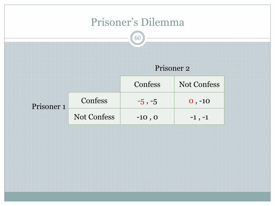
Prisoner’s Dilemma
60
Prisoner 2
Confess Not Confess
Prisoner 1
Confess -5 , -5 0 , -10
Not Confess -10 , 0 -1 , -1
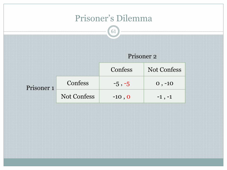
Prisoner’s Dilemma
61
Prisoner 2
Confess Not Confess
Prisoner 1
Confess -5 , -5 0 , -10
Not Confess -10 , 0 -1 , -1
Prisoner’s Dilemma
62
Prisoner 2
Confess Not Confess
Prisoner 1
Confess 0 , -10
Not Confess -10 , 0 -1 , -1
Coordination failure
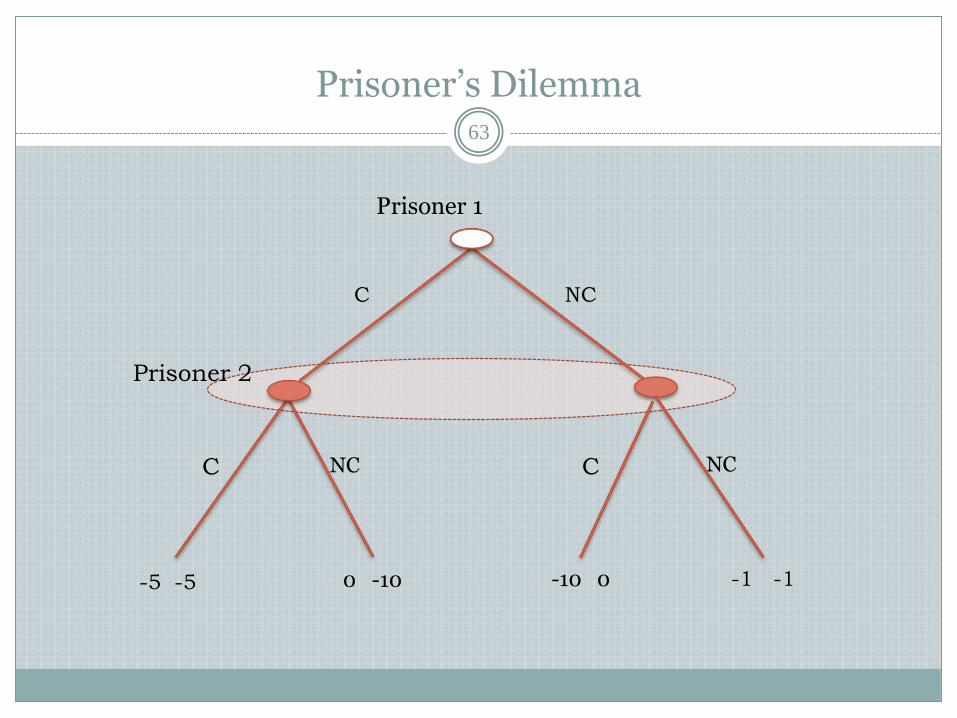
Prisoner’s Dilemma 63
Prisoner 1
Prisoner 2
NC C NC C
NC C
-5 -5 0 -10 -10 0 -1 -1
M U L T I P L E E Q U I L I B R I A
F I R S T M O V E R A D V A N T A G E
64
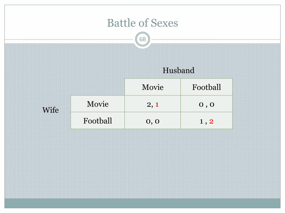
Battle of Sexes
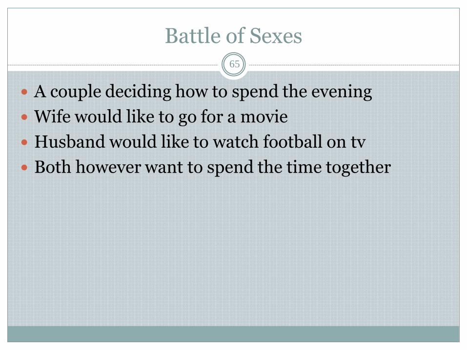
Battle of Sexes 65
A couple deciding how to spend the evening
Wife would like to go for a movie
Husband would like to watch football on tv
Both however want to spend the time together

Battle of Sexes
66
Husband
Movie Football
Wife
Movie 2, 1 0 , 0
Football 0, 0 1 , 2

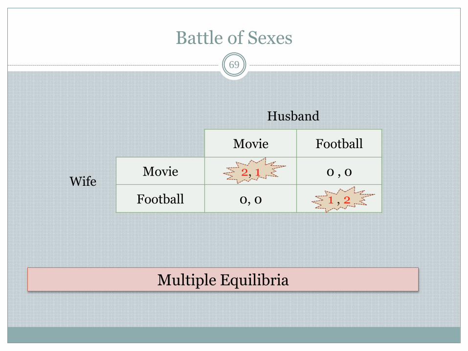
Battle of Sexes
67
Husband
Movie Football
Wife
Movie 2, 1 0 , 0
Football 0, 0 1 , 2
Battle of Sexes
68
Husband
Movie Football
Wife
Movie 2, 1 0 , 0
Football 0, 0 1 , 2
Battle of Sexes
69
Husband
Movie Football
Wife
Movie 2, 1 0 , 0
Football 0, 0 1 , 2
Multiple Equilibria
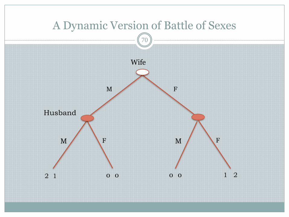
A Dynamic Version of Battle of Sexes 70
Wife
Husband
F M F M
F M
2 1 0 0 0 0 1 2
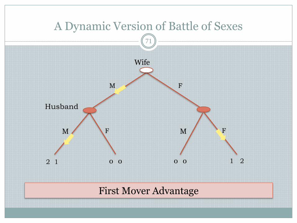
A Dynamic Version of Battle of Sexes 71
Wife
Husband
F M F M
F M
2 1 0 0 0 0 1 2
First Mover Advantage
S T R A T E G I E S I N D Y N A M I C G A M E S
I N C R E D I B L E T H R E A T S
72
Entry Deterrence Game
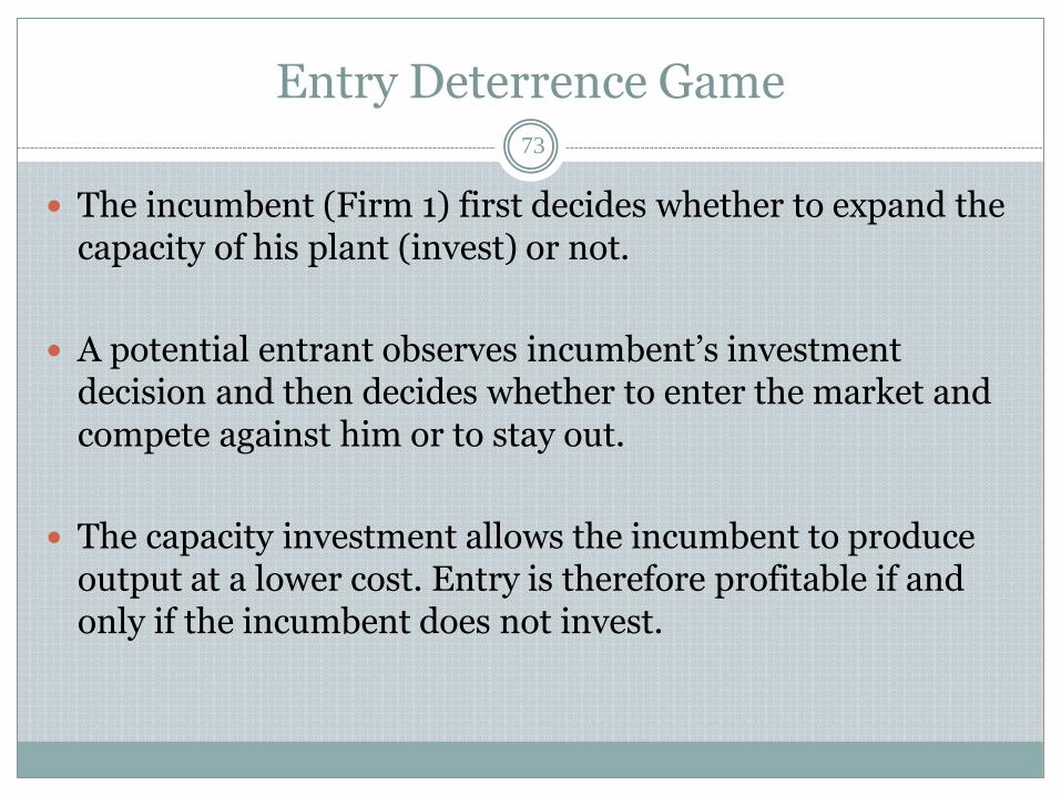
Entry Deterrence Game 73
The incumbent (Firm 1) first decides whether to expand the capacity of his plant (invest) or not.
A potential entrant observes incumbent’s investment decision and then decides whether to enter the market and compete against him or to stay out.
The capacity investment allows the incumbent to produce output at a lower cost. Entry is therefore profitable if and only if the incumbent does not invest.
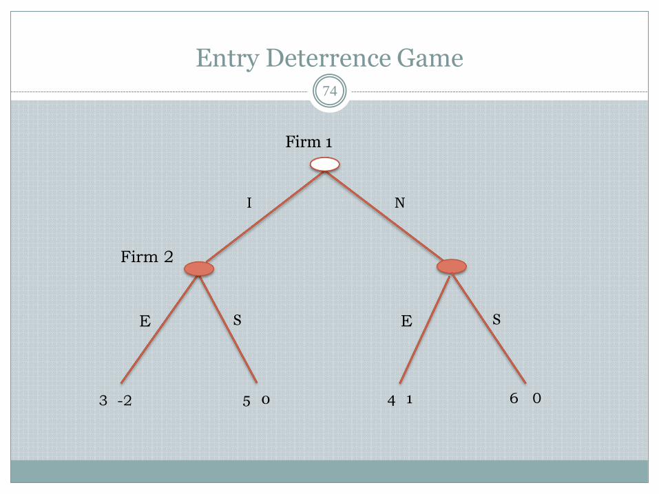
Entry Deterrence Game 74
Firm 1
Firm 2
S E S E
N I
3 -2 5 0 4 1 6 0
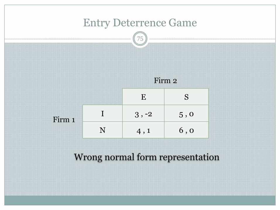
Entry Deterrence Game
75
Firm 2
E S
Firm 1
I 3 , -2 5 , 0
N 4 , 1 6 , 0
Wrong normal form representation
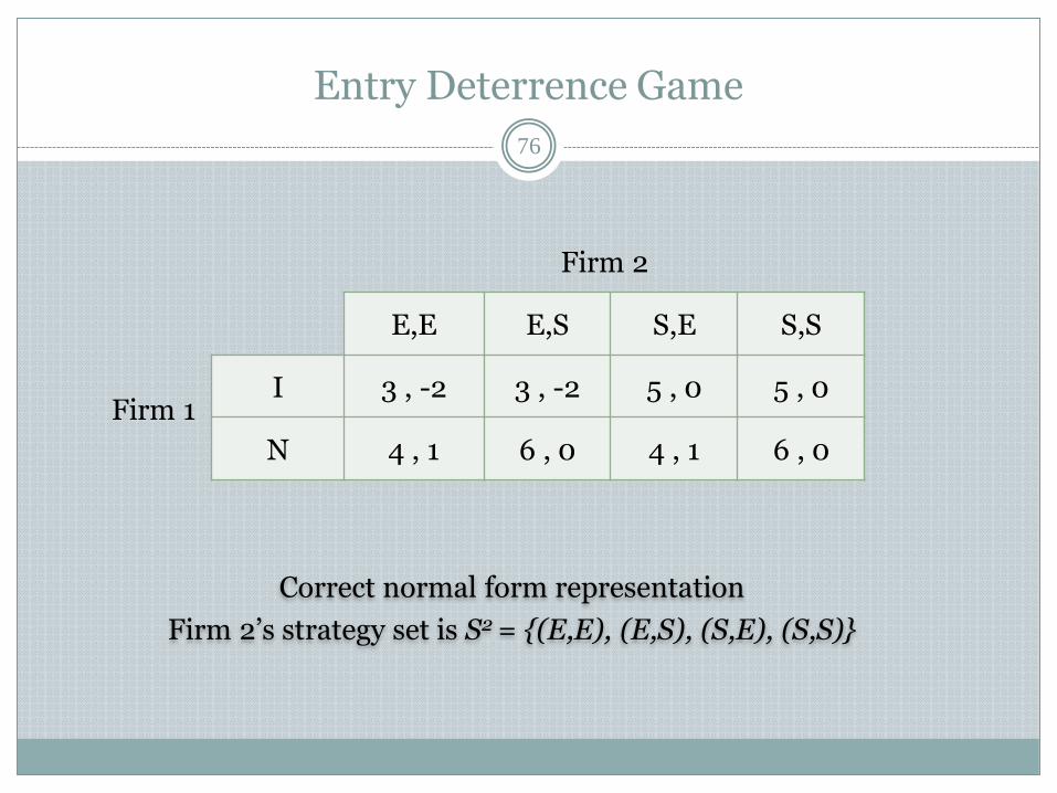
Entry Deterrence Game
76
Firm 2
E,E E,S S,E S,S
Firm 1
I 3 , -2 3 , -2 5 , 0 5 , 0
N 4 , 1 6 , 0 4 , 1 6 , 0
Correct normal form representation
Firm 2’s strategy set is S2 = {(E,E), (E,S), (S,E), (S,S)}
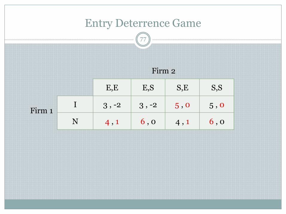
Entry Deterrence Game
77
Firm 2
E,E E,S S,E S,S
Firm 1
I 3 , -2 3 , -2 5 , 0 5 , 0
N 4 , 1 6 , 0 4 , 1 6 , 0
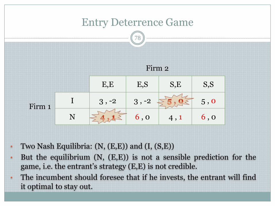
Entry Deterrence Game
78
Firm 2
E,E E,S S,E S,S
Firm 1
I 3 , -2 3 , -2 5 , 0
N 6 , 0 4 , 1 6 , 0
• Two Nash Equilibria: (N, (E,E)) and (I, (S,E))
• But the equilibrium (N, (E,E)) is not a sensible prediction for the game, i.e. the entrant’s strategy (E,E) is not credible.
• The incumbent should foresee that if he invests, the entrant will find it optimal to stay out.
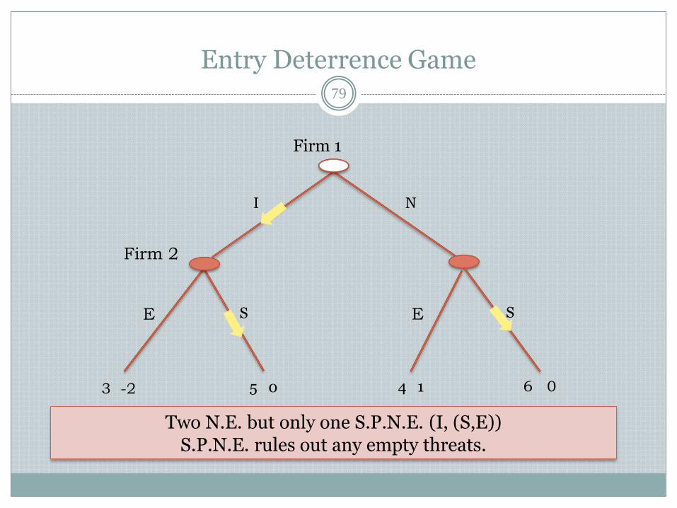
Entry Deterrence Game 79
Firm 1
Firm 2
S E S E
N I
3 -2 5 0 4 1 6 0
Two N.E. but only one S.P.N.E. (I, (S,E)) S.P.N.E. rules out any empty threats.
C O M M I T M E N T
80
Burning Bridge Game
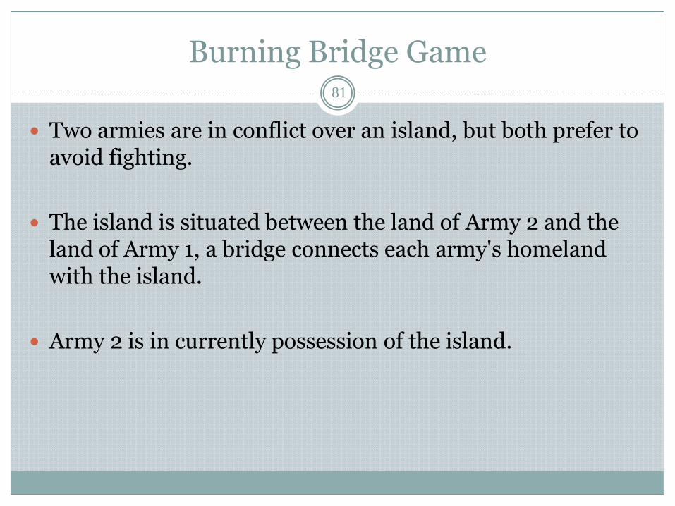
Burning Bridge Game 81
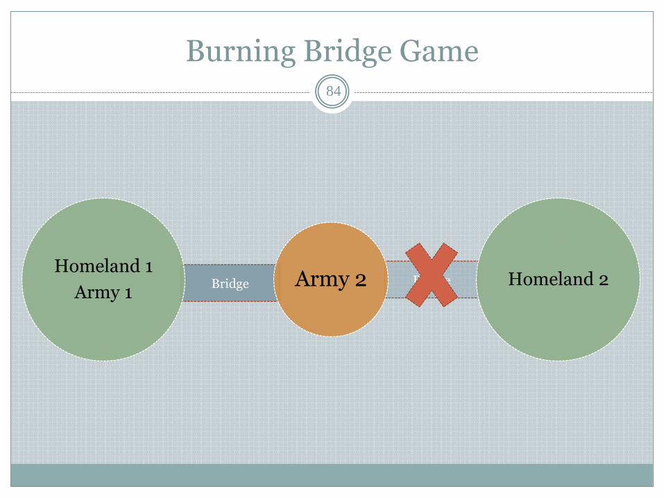
Two armies are in conflict over an island, but both prefer to avoid fighting.
The island is situated between the land of Army 2 and the land of Army 1, a bridge connects each army's homeland with the island.
Army 2 is in currently possession of the island.
Bridge Bridge
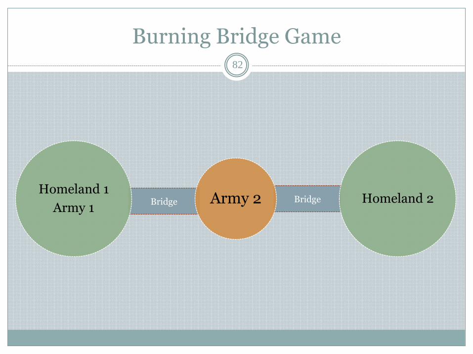
Burning Bridge Game 82
Army 2 Homeland 1
Army 1 Homeland 2
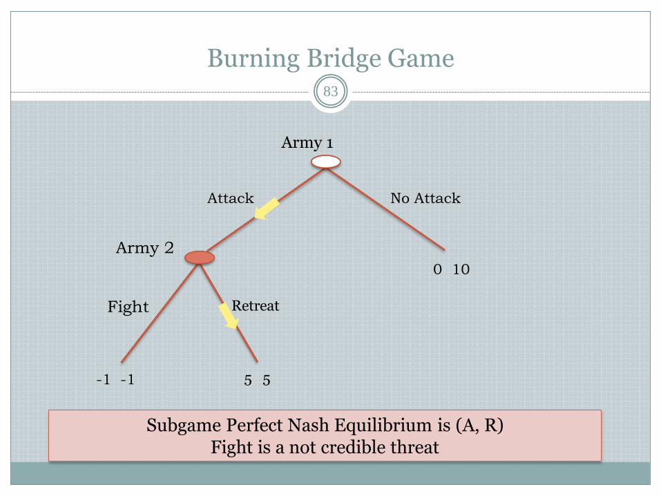
Burning Bridge Game 83
Army 1
Army 2
Retreat Fight
No Attack Attack
-1 -1 5 5
0 10
Subgame Perfect Nash Equilibrium is (A, R) Fight is a not credible threat
Bridge Bridge Army 2 Homeland 1
Army 1 Homeland 2
Burning Bridge Game 84
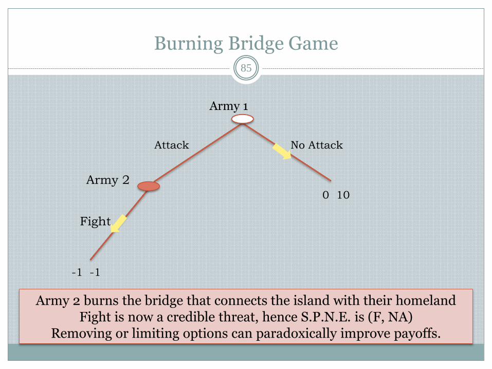
Burning Bridge Game 85
Army 1
Army 2
Fight
No Attack Attack
-1 -1
0 10
Army 2 burns the bridge that connects the island with their homeland Fight is now a credible threat, hence S.P.N.E. is (F, NA)
Removing or limiting options can paradoxically improve payoffs.
86
EXTENSIONS
Mixed Strategies
Mixed strategy: A probability distribution over the pure strategies of a player Since probabilities are continuous, there are infinitely many mixed strategies
available to a player, even if their strategy set is finite. Pure strategies are a degenerate case of a mixed strategy in which that particular
pure strategy is selected with probability 1 and every other strategy with probability 0.
Example: Rock – Paper – Scissors Game Each player simultaneously forms his or her hand into the shape of either a rock,
a piece of paper, or a pair of scissors. Rule: rock beats (breaks) scissors, scissors beats (cuts) paper, and paper beats (covers) rock
No pure strategy Nash Equilibrium One mixed strategy Nash Equilibrium – each player plays rock, paper and
scissors each with 1/3 probability
87
Repeated Games
88
Cooperative Games
89
Mechanism Design
90


