
Introduction to non-linear optimization
Ross A. Lippert
D. E. Shaw Research
February 25, 2008
R. A. Lippert Non-linear optimization

Optimization problems
problem: Let f : Rn → (−∞,∞],
find minx∈Rn
{f (x)}
find x∗ s.t. f (x∗) = minx∈Rn
{f (x)}
Quite general, but some cases, like f convex, are fairly solvable.Today’s problem: How about f : R
n → R, smooth?
find x∗ s.t. ∇f (x∗) = 0
We have a reasonable shot at this if f is twice differentiable.
R. A. Lippert Non-linear optimization
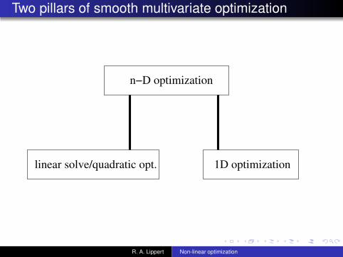
Two pillars of smooth multivariate optimization
n−D optimization
linear solve/quadratic opt. 1D optimization
R. A. Lippert Non-linear optimization
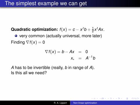
The simplest example we can get
Quadratic optimization: f (x) = c − x t b + 12x tAx .
very common (actually universal, more later)Finding ∇f (x) = 0
∇f (x) = b − Ax = 0x∗ = A−1b
A has to be invertible (really, b in range of A).Is this all we need?
R. A. Lippert Non-linear optimization

Max, min, saddle, or what?
Require A be positive definite, why?
−1−0.5
00.5
1
−1
−0.5
0
0.5
10
0.5
1
1.5
2
2.5
3
−1−0.5
00.5
1
−1
−0.5
0
0.5
1−3
−2.5
−2
−1.5
−1
−0.5
0
−1−0.5
00.5
1
−1
−0.5
0
0.5
1−2
−1.5
−1
−0.5
0
0.5
1
−1−0.5
00.5
1
−1
−0.5
0
0.5
10
0.2
0.4
0.6
0.8
1
R. A. Lippert Non-linear optimization
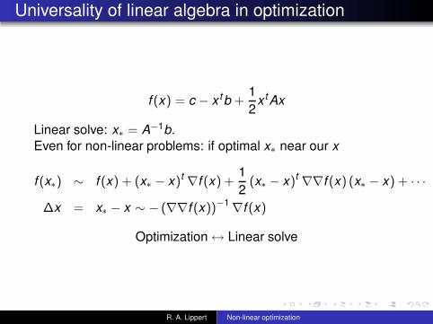
Universality of linear algebra in optimization
f (x) = c − x t b +12x t Ax
Linear solve: x∗ = A−1b.Even for non-linear problems: if optimal x∗ near our x
f (x∗) ∼ f (x) + (x∗ − x)t ∇f (x) +12 (x∗ − x)t ∇∇f (x) (x∗ − x) + · · ·
∆x = x∗ − x ∼ − (∇∇f (x))−1 ∇f (x)
Optimization ↔ Linear solve
R. A. Lippert Non-linear optimization

Linear solve
x = A−1bBut really we just want to solve
Ax = b
Don’t form A−1 if you can avoid it.(Don’t form A if you can avoid that!)
For a general A, there are three important special cases,
diagonal: A =
a1 0 00 a2 00 0 a3
thus xi = 1ai
bi
orthogonal At A = I, thus A−1 = At and x = Atb
triangular: A =
a11 0 0a21 a22 0a31 a32 a33
, xi = 1aii
(
bi −∑
j<i aijxj)
R. A. Lippert Non-linear optimization
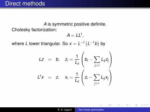
Direct methods
A is symmetric positive definite.Cholesky factorization:
A = LLt ,
where L lower triangular. So x = L−t (
L−1b)
by
Lz = b, zi =1Lii
bi −∑
j<iLijzj
Ltx = z, xi =1Lii
zi −∑
j>iLijxj
R. A. Lippert Non-linear optimization

Direct methods
A is symmetric positive definite.Eigenvalue factorization:
A = QDQt ,
where Q is orthogonal and D is diagonal. Then
x = Q(
D−1 (
Qt b)
)
.
More expensive than ChoeskyDirect methods are usually quite expensive (O(n3) work).
R. A. Lippert Non-linear optimization

Iterative method basics
What’s an iterative method?Definition (Informal definition)An iterative method is an algorithm A which takes what youhave, xi , and gives you a new xi+1 which is less bad such thatx1, x2, x3, . . . converges to some x∗ with badness= 0.
A notion of badness could come from1 distance from xi to our problem solution2 value of some objective function above its minimum3 size of the gradient at xi
e.g. If x is supposed to satisfy Ax = b, we could take ||b − Ax ||to be the measure of badness.
R. A. Lippert Non-linear optimization
Iterative method considerations
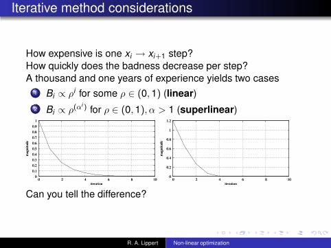
How expensive is one xi → xi+1 step?How quickly does the badness decrease per step?A thousand and one years of experience yields two cases
1 Bi ∝ ρi for some ρ ∈ (0, 1) (linear)2 Bi ∝ ρ(αi ) for ρ ∈ (0, 1), α > 1 (superlinear)
0 0.1 0.2 0.3 0.4 0.5 0.6 0.7 0.8 0.9
1
0 2 4 6 8 10
mag
nitu
de
iteration
0 0.1 0.2 0.3 0.4 0.5 0.6 0.7 0.8 0.9
1
0 2 4 6 8 10
mag
nitu
de
iteration
0
0.2
0.4
0.6
0.8
1
1.2
0 2 4 6 8 10
mag
nitu
de
iteration
0
0.2
0.4
0.6
0.8
1
1.2
0 2 4 6 8 10
mag
nitu
de
iteration
Can you tell the difference?
R. A. Lippert Non-linear optimization

Convergence
1e−04
0.001
0.01
0.1
1
0 2 4 6 8 10
mag
nitu
de
iteration
1e−04
0.001
0.01
0.1
1
0 2 4 6 8 10
mag
nitu
de
iteration
1e−30
1e−25
1e−20
1e−15
1e−10
1e−05
1
100000
0 2 4 6 8 10
mag
nitu
de
iteration
1e−30
1e−25
1e−20
1e−15
1e−10
1e−05
1
100000
0 2 4 6 8 10
mag
nitu
de
iteration
Now can you tell the difference?
1e−30
1e−25
1e−20
1e−15
1e−10
1e−05
1
100000
0 2 4 6 8 10
mag
nitu
de
iteration
1e−30
1e−25
1e−20
1e−15
1e−10
1e−05
1
100000
0 2 4 6 8 10
mag
nitu
de
iteration
When evaluating an iterative method against manufacturer’sclaims, be sure to do semilog plots.
R. A. Lippert Non-linear optimization

Iterative methods
Motivation: directly optimize f (x) = c − x t b + 12x t Ax .
gradient descent:1 Search direction: ri = −∇f = b − Axi2 Search step: xi+1 = xi + αi ri
3 Pick alpha: αi =r ti ri
r ti Ari
minimizes f (x + αri )
f (xi + αri ) = c − x ti b +
12x t
i Axi + αr ti (Axi − b) +
12α2r t
i Ari
= f (xi) − αr ti ri +
12α2r t
i Ari
(Cost of a step = 1 A-multiply.)
R. A. Lippert Non-linear optimization

Iterative methods
Optimize f (x) = c − x t b + 12x tAx .
conjugate gradient descent:1 Search direction: di = ri + βidi−1, with ri = b − Axi .2 Pick βi = − d t
i−1Arid t
i−1Adi−1, ensures d t
i−1Adi = 0.3 Search step: xi+1 = xi + αidi
4 Pick αi =d t
i rid t
i Adi: minimizes f (xi + αdi)
f (xi + αdi) = c − x ti b +
12x t
i Axi − αd ti ri +
12α2d t
i Adi
(also means that r ti+1di = 0)
Avoid extra A-multiply: using Adi−1 ∝ ri−1 − riβi = − (ri−1−ri)t ri
(ri−1−ri)t di−1= − (ri−1−ri)t ri
r ti−1di−1
=(ri−ri−1)t ri
r ti−1ri−1
R. A. Lippert Non-linear optimization

A cute result
conjugate gradient descent:1 ri = b − Axi2 Search direction: di = ri + βidi−1 (β s.t. diAdi−1 = 0)3 Search step: xi+1 = xi + αidi (α minimizes).
Cute result (not that useful in practice)
Theorem (sub-optimality of CG)(Assuming x0 = 0) at the end of step k, the solution xk is theoptimal linear combination of b, Ab, A2b, . . . Akb for minimizing
c − btx +12x tAx .
(computer arithmetic errors make this less than perfect)Very little extra effort. Much better convergence.
R. A. Lippert Non-linear optimization
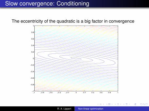
Slow convergence: Conditioning
The eccentricity of the quadratic is a big factor in convergence
−1 −0.8 −0.6 −0.4 −0.2 0 0.2 0.4 0.6 0.8 1−1
−0.8
−0.6
−0.4
−0.2
0
0.2
0.4
0.6
0.8
1
R. A. Lippert Non-linear optimization

Convergence and eccentricity
κ =max eig(A)
min eig(A)
For gradient descent,
||ri || ∼∣
∣
∣
∣
κ − 1κ + 1
∣
∣
∣
∣
i
For CG,
||ri || ∼∣
∣
∣
∣
√κ − 1√κ + 1
∣
∣
∣
∣
i
useless CG fact: in exact arithmetic ri = 0 when i > n (A isn × n).
R. A. Lippert Non-linear optimization

The truth about descent methods
Very slow unless κ can be controlled.How do we control κ?
Ax = b → (PAP t)y = Pb, x = P t y
where P is a pre-conditioner you pick.How to make κ(PAP t) small?
perfect answer, P = L−1 where LtL = A (Choleskyfactorization).imperfect answer, P ∼ L−1
Variations on the theme of incomplete factorization:P−1 = D 1
2 where D = diag (a11, . . . , ann)
more generally, incomplete Cholesky decompositionsome easy nearby solution or simple approximate A(requiring domain knowledge)
R. A. Lippert Non-linear optimization
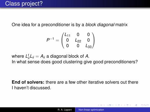
Class project?
One idea for a preconditioner is by a block diagonal matrix
P−1 =
L11 0 00 L22 00 0 L33
where LtiiLii = Aii a diagonal block of A.
In what sense does good clustering give good preconditioners?
End of solvers: there are a few other iterative solvers out thereI haven’t discussed.
R. A. Lippert Non-linear optimization
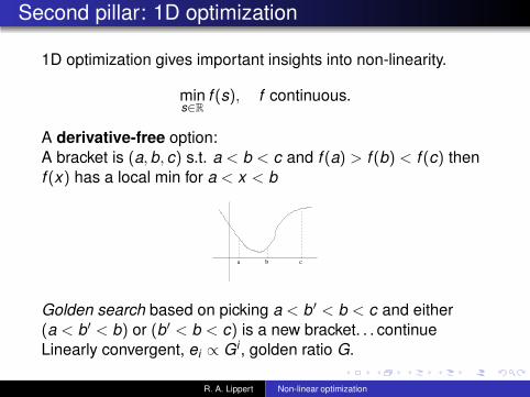
Second pillar: 1D optimization
1D optimization gives important insights into non-linearity.
mins∈R
f (s), f continuous.
A derivative-free option:A bracket is (a, b, c) s.t. a < b < c and f (a) > f (b) < f (c) thenf (x) has a local min for a < x < b
a b c
Golden search based on picking a < b′ < b < c and either(a < b′ < b) or (b′ < b < c) is a new bracket. . . continueLinearly convergent, ei ∝ Gi , golden ratio G.
R. A. Lippert Non-linear optimization

1D optimization
Fundamentally limited accuracy of derivative-free argmin:
a b c
Derivative-based methods, f ′(s) = 0, for accurate argminbracketed: (a, b) s.t. f ′(a), f ′(b) opposite sign
1 bisection (linearly convergent)2 modified regula falsi & Brent’s method (superlinear)
unbracketed:1 secant method (superlinear)2 Newton’s method (superlinear; requires another derivative)
R. A. Lippert Non-linear optimization
From quadratic to non-linear optimizations
What can happen when far from the optimum?−∇f (x) always points in a direction of decrease∇∇f (x) may not be positive definite
For convex problems ∇∇f is always positive semi-definite andfor strictly convex it is positive definite.What do we want?
find a convex neighborhood of x∗ (be robust againstmistakes)apply a quadratic approximation (do linear solve)
Fact: ∀ non-linear optimization algorithms, ∃f which fools it.
R. A. Lippert Non-linear optimization
Naïve Newton’s method
Newton’s method finding x s.t. ∇f (x) = 0
∆xi = − (∇∇f (xi))−1 ∇f (xi)
xi+1 = xi + ∆xi
Asymptotic convergence, ei = xi − x∗∇f (xi) = ∇∇f (x∗)ei + O(||ei ||2)
∇∇f (xi) = ∇∇f (x∗) + O(||ei ||)ei+1 = ei − (∇∇fi)−1 ∇fi = O(||ei ||2)
“squares the error” at every step (exactly eliminates the linearerror).
R. A. Lippert Non-linear optimization

Naïve Newton’s method
Sources of trouble1 if ∇∇f (xi) not posdef, ∆xi = xi+1 − xi might be in an
increasing direction.2 if ∇∇f (xi) posdef, (∇f (xi))
t ∆xi < 0 so ∆xi is a direction ofdecrease (could overshoot)
3 even if f is convex, f (xi+1) ≤ f (xi ) not assured.(f (x) = 1 + ex + log(1 + e−x) starting from x = −2).
4 if all goes well, superlinear convergence!
R. A. Lippert Non-linear optimization

1D example of Newton trouble
1D example of trouble: f (x) = x 4 − 2x2 + 12x
−20
−15
−10
−5
0
5
10
15
20
−2 −1.5 −1 −0.5 0 0.5 1 1.5−20
−15
−10
−5
0
5
10
15
20
−2 −1.5 −1 −0.5 0 0.5 1 1.5
Has one local minimumIs not convex (note the concavity near x=0)
R. A. Lippert Non-linear optimization

1D example of Newton trouble
derivative of trouble: f ′(x) = 4x3 − 4x + 12
−15
−10
−5
0
5
10
15
20
−2 −1.5 −1 −0.5 0 0.5 1 1.5−15
−10
−5
0
5
10
15
20
−2 −1.5 −1 −0.5 0 0.5 1 1.5the negative f ′′ region around x = 0 repels the iterates:0 → 3 → 1.96154 → 1.14718 → 0.00658 → 3.00039 → 1.96182 →1.14743 → 0.00726 → 3.00047 → 1.96188 → 1.14749 → · · ·
R. A. Lippert Non-linear optimization

Non-linear NewtonTry to enforce f (xi+1) ≤ f (xi)
∆xi = − (λI + ∇∇f (xi))−1 ∇f (xi)
xi+1 = xi + αi∆xi
Set λ > 0 to keep ∆xi in a direction of decrease (manyheuristics).Pick αi > 0 such that f (xi + αi∆xi) ≤ f (xi). If ∆xi is a directionof decrease, some αi exists.
1D-minimization do 1D optimization problem,
minαi∈(0,β]
f (xi + αi∆xi)
Armijo-search use this rule: αi = ρµn some n
f (xi + s∆xi) − f (xi) ≤ νs (∆xi)t ∇f (xi)
with ρ, µ, ν fixed (e.g. ρ = 2, µ = ν = 12 ).
R. A. Lippert Non-linear optimization

Line searching
1D-minimization looks like less of a hack than Armijo. ForNewton, asymptotic convergence is not strongly affected, andfunction evaluations can be expensive.
far from x∗ their only value is ensuring decreasenear x∗ the methods will return αi ∼ 1.
If you have a Newton step, accurate line-searching adds littlevalue.
R. A. Lippert Non-linear optimization

Practicality
Direct (non-iterative, non-structured) solves are expensive!∇∇f information is often expensive!
R. A. Lippert Non-linear optimization
Iterative methods
gradient descent:1 Search direction: ri = −∇f (xi)2 Search step: xi+1 = xi + αi ri3 Pick alpha: (depends on what’s cheap)
1 linearized αi =r ti (∇∇f )ri
r ti ri
2 minimization f (xi + αri) (danger: low quality)3 zero-finding r t
i ∇f (xi + αri) = 0
R. A. Lippert Non-linear optimization

Iterative methods
conjugate gradient descent:1 Search direction: di = −ri + βidi−1, with ri = −∇f (xi).2 Pick βi without ∇∇f
1 βi =(ri−ri−1)
t ri−1(ri−ri−1)t ri
(Polak-Ribiere)2 can also use βi =
r ti ri
r ti−1ri−1
(Fletcher-Reeves)
3 Search step: xi+1 = xi + αidi1 linearized αi =
d ti (∇∇f )di
r ti di
2 1D minimization f (xi + αdi ) (danger: low quality)3 zero-finding d t
i ∇f (xi + αdi ) = 0
R. A. Lippert Non-linear optimization
Don’t forget the truth about iterative methods
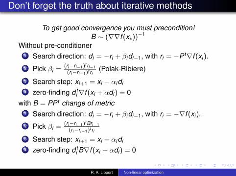
To get good convergence you must precondition!B ∼ (∇∇f (x∗))−1
Without pre-conditioner1 Search direction: di = −ri + βidi−1, with ri = −P t∇f (xi).2 Pick βi =
(ri−ri−1)t ri−1(ri−ri−1)t ri
(Polak-Ribiere)3 Search step: xi+1 = xi + αidi4 zero-finding d t
i ∇f (xi + αdi) = 0with B = PP t change of metric
1 Search direction: di = −ri + βidi−1, with ri = −∇f (xi).2 Pick βi =
(ri−ri−1)tBri−1(ri−ri−1)t ri
3 Search step: xi+1 = xi + αidi4 zero-finding d t
i B∇f (xi + αdi) = 0
R. A. Lippert Non-linear optimization

What else?
Remember this cute property?
Theorem (sub-optimality of CG)(Assuming x0 = 0) at the end of step k, the solution xk is theoptimal linear combination of b, Ab, A2b, . . . Akb for minimizing
c − btx +12x tAx .
In a sense, CG learns about A from the history of b − Axi .Noting,
1 computer arithmetic errors ruin this nice property quickly2 non-linearity ruins this property quickly
R. A. Lippert Non-linear optimization
Quasi-Newton
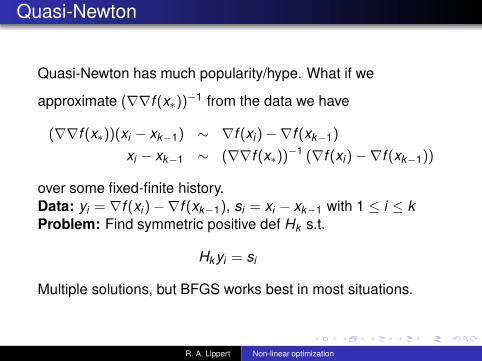
Quasi-Newton has much popularity/hype. What if we
approximate (∇∇f (x∗))−1 from the data we have
(∇∇f (x∗))(xi − xk−1) ∼ ∇f (xi) −∇f (xk−1)
xi − xk−1 ∼ (∇∇f (x∗))−1 (∇f (xi) −∇f (xk−1))
over some fixed-finite history.Data: yi = ∇f (xi) −∇f (xk−1), si = xi − xk−1 with 1 ≤ i ≤ kProblem: Find symmetric positive def Hk s.t.
Hk yi = si
Multiple solutions, but BFGS works best in most situations.
R. A. Lippert Non-linear optimization

BFGS update
Hk =
(
I − sk y tk
y tk sk
)
Hk−1
(
I − yk stk
y tk sk
)
+sk st
ky t
k sk
LemmaThe BFGS update minimizes minH ||H−1 − H−1
k−1||2F such thatHyk = sk .
Forming Hk not necessary, e.g. Hk v can be recursivelycomputed.
R. A. Lippert Non-linear optimization

Quasi-Newton
Typically keep about 5 data points in the history.initialize Set H0 = I, r0 = −∇f (x0), d0 = r0 goto 3
1 Compute rk = −∇f (xk ), yk = rk−1 − rk2 Compute dk = Hk rk3 Search step: xk+1 = xk + αk dk (line-search)
Asymptotically identical to CG (with αi =d t
i (∇∇f )dir ti di
)Armijo line searching has good theoretical properties. Typicallyused.Quasi-Newton ideas generalize beyond optimization (e.g.fixed-point iterations)
R. A. Lippert Non-linear optimization
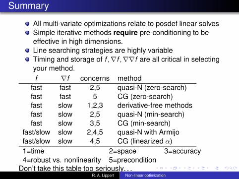
SummaryAll multi-variate optimizations relate to posdef linear solvesSimple iterative methods require pre-conditioning to beeffective in high dimensions.Line searching strategies are highly variableTiming and storage of f ,∇f ,∇∇f are all critical in selectingyour method.f ∇f concerns method
fast fast 2,5 quasi-N (zero-search)fast fast 5 CG (zero-search)fast slow 1,2,3 derivative-free methodsfast slow 2,5 quasi-N (min-search)fast slow 3,5 CG (min-search)
fast/slow slow 2,4,5 quasi-N with Armijofast/slow slow 4,5 CG (linearized α)1=time 2=space 3=accuracy4=robust vs. nonlinearity 5=precondition
Don’t take this table too seriously. . .R. A. Lippert Non-linear optimization


