
Introduction to the P5 Computing Laboratory
Eric Peasley
Department of Engineering Science

Design, Build and Test
Session 3, DBT Part A
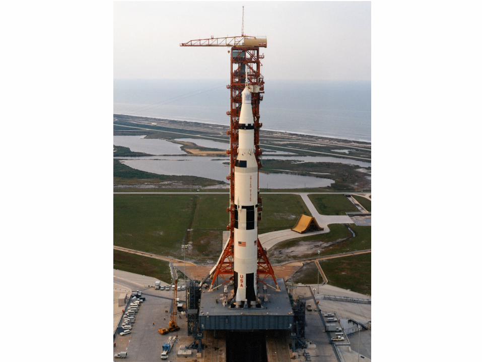
Simulating a Rocket Launch
Informal Assessment (No marks)
Session 4 & 5, DBT Part B
The Lander Controller
Assessment (15 marks)

What to do before Session 3
● Read the Introduction page 107 to 110
● Read Euler's Method 111 to 114

What to do before Session 3If you want to get started
● Work your way through the rest of the Euler section on page 115 to 117
● Read Exercise introduction 118 to 121
● The Exercises must be done in the Laboratory session

Program Design
● To make is easier to write large programs
● To improve the quality of your code
a) How well your code works
b) How understandable your code is


What is the purpose ofComments
Documentation

Final_Velocity = Initial_Velocity + acceleration * time;
Distance = Initial_Velocity * time + (acceleration *time.^2)/2;
Final_Velocity = sqrt(Initial_Velocity.^2 + 2*acceleration*Distance);
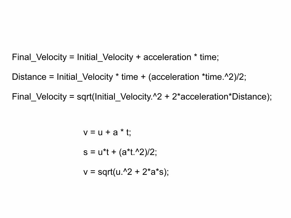
v = u + a * t;
s = u*t + (a*t.^2)/2;
v = sqrt(u.^2 + 2*a*s);
Final_Velocity = Initial_Velocity + acceleration * time;
Distance = Initial_Velocity * time + (acceleration *time.^2)/2;
Final_Velocity = sqrt(Initial_Velocity.^2 + 2*acceleration*Distance);

v = u + a * t;
s = u*t + (a*t.^2)/2;
v = sqrt(u.^2 + 2*a*s);
% u = The initial velocity in m/s % v = The final velocity in m/s% a = The constant acceleration m/s^2;% t = The time duration in seconds;% s = The distance travelled in metres
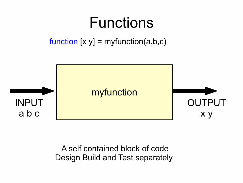
Functions
myfunction
function [x y] = myfunction(a,b,c)
INPUTa b c
OUTPUTx y
A self contained block of codeDesign Build and Test separately

The problems with LARGE programs
● The larger the program,
the more errors you get.
● The more code you have, the more difficult it is to find the errors.

The problems with LARGE programs
Program Size

How to write BIG Programs
Prog1 1 day
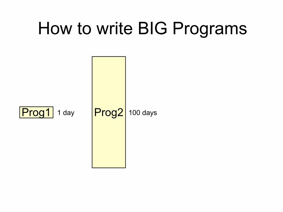
How to write BIG Programs
Prog1 Prog21 day 100 days

How to write BIG Programs
Prog1 Prog2
fnfnfnfnfnfnfnfnfnfn
1 day
1 day
1 day
1 day
1 day
1 day
1 day
1 day
1 day
1 day
Total10 days
1 day 100 days

Car Body Engine Gear Box Transmission Brakes Wheels etc

Car Body Engine Gear Box Transmission Brakes Wheels etc
Engine Pistons Crank Electrical System Cooling System Fuel Delivery etc

Car Body Engine Gear Box Transmission Brakes Wheels etc
Engine Pistons Crank Electrical System Cooling System Fuel Delivery etc
Cooling System Radiator Fan Water Pump etc
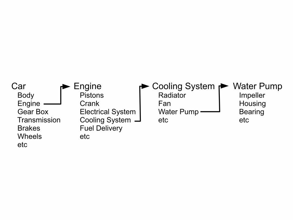
Car Body Engine Gear Box Transmission Brakes Wheels etc
Engine Pistons Crank Electrical System Cooling System Fuel Delivery etc
Cooling System Radiator Fan Water Pump etc
Water Pump Impeller Housing Bearing etc

Programs
Function
Function Function Function Function
Function
Function
Function
Function Function
Function
Function
Program
Function

Top Down Design

Structures
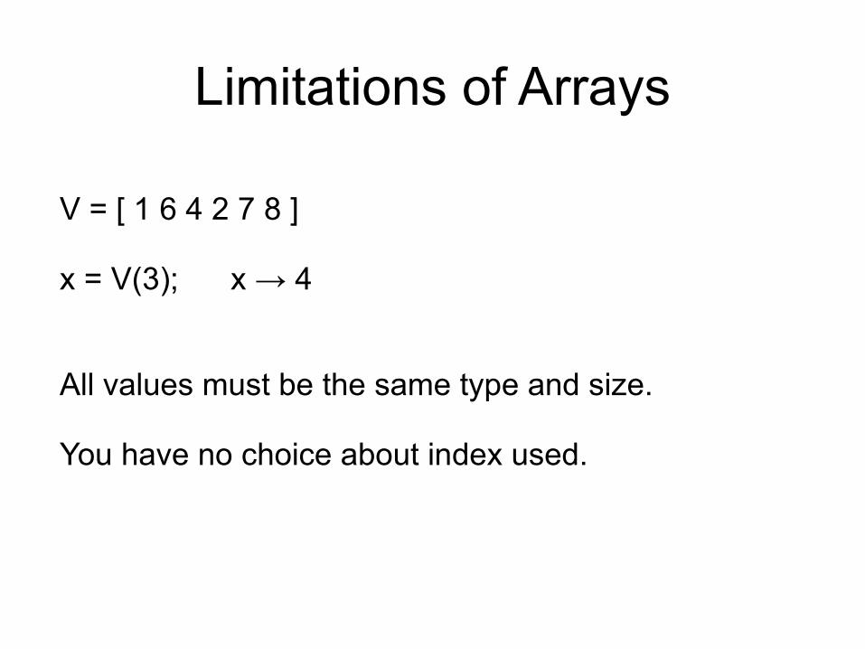
V = [ 1 6 4 2 7 8 ]
x = V(3); x → 4
All values must be the same type and size.
You have no choice about index used.
Limitations of Arrays
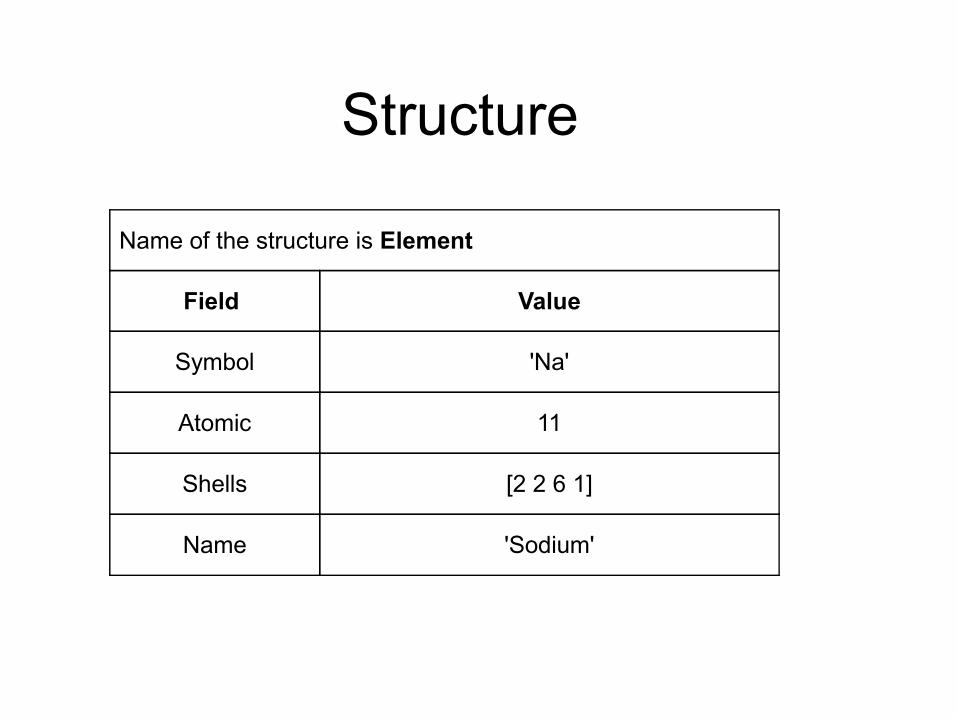
Name of the structure is Element
Field Value
Symbol 'Na'
Atomic 11
Shells [2 2 6 1]
Name 'Sodium'
Structure

Structure.Field = Value
Element.Symbol = 'Na';
Element.Atomic = 11; Element.Shells = [2 2 6 1];
Element.Name = 'Sodium';
Structure

%SquareHouse(1).path = [0 100 100 0 0 0 0 100 100 0]; % squareHouse(1).colour = 'r'; % The colour to plotHouse(1).solid = 1; % Fill the square %TriangleHouse(2).path = [ -20 50 120 -20 100 170 100 100 ]; % TriangleHouse(2).colour = 'g'; % The colour to plotHouse(2).solid = 1; % Fill the triangle
Structural ArrayEvery element of the array contains a structure

rotatepicabout rotateabout
Translate
rotate
House
House(1) path col solid
House(2) path col solid
House(3) path col solid
““
““
““
““
House(92) path col solid
Functions
Structural Array
Programming is easier if you organise your data and code
Simulating a Rocket Launch

Saturn V Rocket

0 20 40 60 80 100 120 140 160
0
20
40
60
80
100
120
140
160

Real World Problem
mdvdt
= Th(t ) − k v2 − m g

Real World Problem
mdvdt
= Th(t ) − k v2 − m g
dvdt
=Th(t ) − k v2
m(t )− g

dydt
= f (t , y) y ( t 0)= y0
Initial Value Problem
Find y (t )when
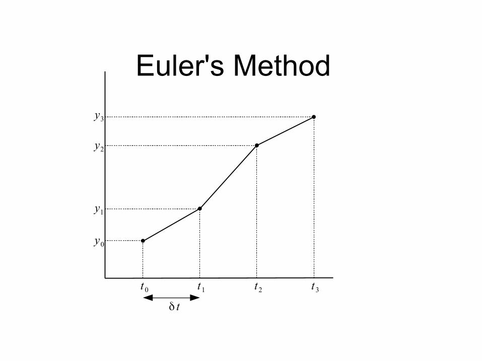
Euler's Method
t 0 t1
δ t
y0
y1
t2 t 3
y2
y3

t0 t1
δ t
y0
y1
What is the slope of the line ?

t0 t1
δ t
y0
y1Slope=
y1− y0t 1−t 0
=y1− y0δ t
What is the slope of the line ?

What is ?dydt

What is ?dydt
dydt
= k = slope

t0 t1
δ t
y0
dydt
= f (t , y) y (t 0)= y0

t0 t1
δ t
y0
dydt
= f (t , y) y (t 0)= y0
dydt
(t 0) = f (t0, y0)

t0 t1
δ t
y0
dydt
= f (t , y) y (t 0)= y0
dydt
(t 0) = f (t0, y0)
slope = f (t0, y0)

t0 t1
δ t
y0
y1
dydt
= f (t , y) y (t 0)= y0
dydt
(t 0) = f (t0, y0)
y1− y0δ t
= f (t0, y0)
slope = f (t0, y0)

t0 t1
δ t
y0
y1
dydt
= f (t , y) y (t 0)= y0
dydt
(t 0) = f (t0, y0)
y1− y0 = δ t f ( t 0, y0)
y1− y0δ t
= f (t0, y0)
slope = f (t0, y0)

t0 t1
δ t
y0
y1
dydt
= f (t , y) y (t 0)= y0
dydt
(t 0) = f (t0, y0)
y1− y0 = δ t f ( t 0, y0)
y1− y0δ t
= f (t0, y0)
slope = f (t0, y0)
y1= y0+δ t f ( t 0, y0)

dydt
= f (t , y) y (t 0)= y0
y1= y0+δ t f ( t 0, y0)
t0 t 1
δ t
y0
y1
t2 t 3

dydt
= f (t , y) y (t 0)= y0
y1= y0+δ t f ( t 0, y0)
t 0 t1
δ t
y0
y1
t 2 t3
y2y2= y1+δ t f ( t1, y1)

dydt
= f (t , y) y (t 0)= y0
y1= y0+δ t f ( t 0, y0)
t0 t 1
δ t
y0
y1
t 2 t 3
y2
y3
y2= y1+δ t f ( t1, y1)
y3= y2+δ t f (t 2, y2)

Using Euler's method to solve y'(t) = f(t,y) y(0) = y0
1. Initialize the values.
2. Repeat for each time step.
3. Store the current values for plotting later.
4. Evaluate the current value of f(t,y).
5. User Euler's formula to evaluate y for the next step. y = y + dt*f(t,y)
6. End of repeat.
7. Plot the date.
Top Down Design of Euler's Method

The Design Cycle

Design
Start with a simple design
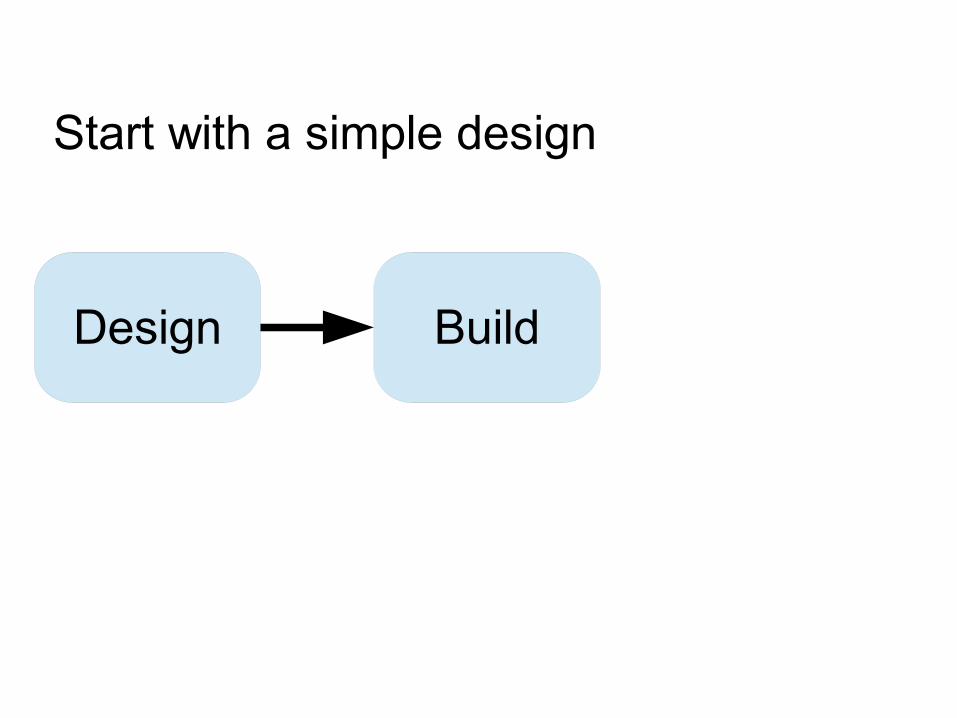
Design Build
Start with a simple design

Design Build Test
Start with a simple design

Design Build Test
Debug
Start with a simple design

Design Build Test
Debug
Make the design more complex

Design Build Test
Debug
Make the design more complex

Design Build Test
Debug
Make the design more complex

Design Build Test
Debug
Make the design more complex

Design Build Test
Debug
Add additional feature to the design

Saturn V Rocket

Design Build Test
Debug
Constant Acceleration

Design Build Test
Debug
Constant Acceleration

Constant Acceleration
dvdt
= a wherea is a constant
v = u+at
s = ut+12at2

Design Build Test
Debug
Thrust Stops after 150 seconds

Thrust Stops after 150 seconds
dvdt
= a
v = u+at
s = ut+12at2
t < 150
dvdt
=−g
v = u−g t
s = ut−12g t2
t ≥ 150

Design Build Test
Debug
Variable Mass

Design Build Test
Debug
Force of Drag

Assessment
No formal assessment for session 3
Get a demonstrator to comment on your program

READ PAGE 119
How to get GOOD MARKS

Practice 2

Debugging


