
Influence of Langmuir Circulation on the Deepening of the Wind-Mixed Layer
YIGN NOH AND GAHYUN GOH
Department of Atmospheric Sciences, and Global Environmental Laboratory, Yonsei University, Seoul, South Korea
SIEGFRIED RAASCH
Institute of Meteorology and Climatology, University of Hannover, Hannover, Germany
(Manuscript received 26 April 2010, in final form 21 November 2010)
ABSTRACT
Analysis of large eddy simulation data reveals that Langmuir circulation (LC) induces a significant en-
hancement of the mixed layer deepening, only if the mixed layer depth (MLD) h is shallow and the buoyancy
jump across it DB is small, when simulations are initiated by applying the wind stress to a motionless mixed
layer with stratification. The difference in the entrainment rate between the cases with and without LC de-
creases with hDB/yL2, where yL is the velocity scale of LC. The ratio of the mixing length scale l between the
cases with and without LC is close to 1 for larger Rt [5(Nl0/q)2; Rt . ;1], but it increases to above 10 with the
decrease of Rt, where N is the Brunt–Vaisala frequency and q and l0 are the velocity and length scales of
turbulence in the homogeneous layer. It is also found that, in the presence of LC, the effect of stratification on
vertical mixing should be parameterized in terms of Rt instead of Ri (5(N/S)2), because velocity shear S is no
longer a dominant source of turbulence. The parameterization is provided by l/l0 5 (1 1 aRt)21/2 with a ; 50,
regardless of the presence of LC. However, LC makes l0 much larger than conventionally used for the
boundary layer.
1. Introduction
Langmuir circulation (LC), which appears in the form
of an array of alternating horizontal roll vortices with
axes aligned roughly with the wind, represents one of the
most important characteristics of the ocean mixed layer
(see, e.g., Leibovich 1983; Smith 2001; Thorpe 2004). The
prevailing theory of LC is that of Craik and Leibovich
(1976), which describes the formation of LC in terms of
instability brought on by the interaction of the Stokes drift
with the wind-driven surface shear current. The instability
is initiated by an additional ‘‘vortex force’’ term in the
momentum equation as us 3 v, where us is the Stokes
drift velocity and v is vorticity.
Various features of LC have been reported from field
observations (Weller and Price 1988; Plueddemann et al.
1996; Smith 1992, 1998; D’Asaro and Dairiki 1997;
Thorpe et al. 2003; Gargett and Wells 2007). Meanwhile,
recent progress in large eddy simulation (LES) has en-
abled us to investigate the dynamical process of LC di-
rectly (Skyllingstad and Denbo 1995; McWilliams et al.
1997; Noh et al. 2004; Min and Noh 2004; Polton and
Belcher 2007; Li et al. 2005; Tejada-Martınez and
Grosch 2007; Grant and Belcher 2009; Sullivan et al.
2007; Harcourt and D’Asaro 2008; Gerbi et al. 2009).
The significance of LC in the ocean mixed layer can
be represented by the turbulent Langmuir number La
[5(u*/Us)1/2], where u* is the frictional velocity and Us is
the Stokes drift velocity at the surface (McWilliams et al.
1997). In particular, Li et al. (2005) and Grant and Belcher
(2009) found that the transition between Langmuir turbu-
lence and shear turbulence occurs at La ; 0.5–2. The ve-
locity of LC yL is shown to scale as yL ; (Usu*2)1/3 (Min and
Noh 2004; Skyllingstad 2001; Harcourt and D’Asaro 2008;
Grant and Belcher 2009), although there are observational
evidences suggesting different scaling (Plueddemann et al.
1996; Smith 1998). In the presence of LC, vertical turbulent
kinetic energy (TKE) is enhanced, and TKE production is
dominated by the divergence of TKE flux, rather than
shear production, in the mixed layer (McWilliams et al.
1997; Noh et al. 2004, 2009; Li et al. 2005; Polton and
Belcher 2007; Gerbi et al. 2009).
Corresponding author address: Yign Noh, Department of At-
mospheric Sciences/Global Environmental Laboratory, Yonsei
University, 262 Seongsanno, Seodaemun-gu, Seoul 120-749, South
Korea.
E-mail: [email protected]
472 J O U R N A L O F P H Y S I C A L O C E A N O G R A P H Y VOLUME 41
DOI: 10.1175/2010JPO4494.1
� 2011 American Meteorological Society

It has been well established that, within the mixed
layer, LC enhances vertical mixing greatly, resulting in the
uniform profiles of temperature and velocity (McWilliams
et al. 1997; Noh et al. 2004; Li et al. 2005; Skyllingstad
2005). Nonetheless, the question of how the mixed layer
deepening is affected by the presence of LC still remains
to be resolved. Evidence of enhancements to mixed layer
deepening or entrainment at the mixed layer depth (MLD)
in the presence of LC has been reported (Li et al. 1995;
Sullivan et al. 2007; Grant and Belcher 2009; Kukulka et al.
2009). On the other hand, Weller and Price (1988) and
Thorpe et al. (2003) observed no evidence that LC has
a direct role in the mixed layer deepening. Skyllingstad
et al. (2000) suggested from the LES results that the effects
of LC are mostly confined to the initial stages of mixed
layer growth.
Note that, in the presence of LC, the transport of heat
and momentum can occur by means of large-scale eddies,
contrary to the wall boundary layer dominated by small-
scale shear-driven eddies near the wall. From this perspec-
tive, large-scale eddies associated with LC can be regarded
as behaving similarly to convective eddies. However, unlike
convective eddies, which are driven continuously by buoy-
ancy force, eddies generated by LC are essentially unforced
and behave inertially, because the vortex force is confined
to near the surface by the decay scale of the Stokes drift.
The intensity of these eddies thus decreases rapidly with
depth, unlike convective eddies.
In spite of uncertainty as to the role of LC in the mixed
layer deepening, there have been several attempts to
incorporate its effects into the mixed layer model (Li
et al. 1995; Li and Garrett 1997; D’Alessio et al. 1998;
Smith 1998; McWilliams and Sullivan 2000; Smyth et al.
2002; Kantha and Clayson 2004). They considered the
modification of the criterion at the MLD controlling the
mixed layer deepening (Li and Garrett 1997; Smith
1998; D’Alessio et al. 1998), the inclusion of nonlocal
mixing by LC (McWilliams and Sullivan 2000; Smyth
et al. 2002), or the increase of TKE (D’Alessio et al.
1998; Kantha and Clayson 2004).
To evaluate and improve the mixed layer models,
however, it is essential to understand properly the phys-
ical process by which LC influences the mixed layer
deepening. Therefore, in the present work, we carried out
LES experiments of the wind-mixed layer deepening
under various conditions and analyzed the results with an
aim to resolve the question on the role of LC in the mixed
layer deepening and to provide information for the pa-
rameterization of its effect.
2. Simulation
The LES model used in the present simulation is
similar to those used in Noh et al. (2004, 2006, 2009,
2010), Min and Noh (2004), and Noh and Nakada
(2010), which have been developed based on the Par-
allelized LES Model (PALM) (Raasch and Schroter
2001). Langmuir circulation is realized by the Craik–
Leibovich vortex force (Craik and Leibovich 1976), and
wave breaking is represented by stochastic forcing. For
simplicity, we assumed that both the wind stress and
wave fields are in the x direction and further assumed
that the wave field is steady and monochromatic. The
associated Stokes velocity is then given by us 5
Us exp(24pz/l) with Us 5 (2pa/l)2(gl/2p)1/2, where a is
the wave height, l is the wavelength, and g is the gravi-
tational acceleration.
Integration is initiated by applying the wind stress to
a motionless fluid. The wind stress at the surface is given
by u* 5 0.02 m s21, and no heat flux is applied at the
surface. The initial MLD is set to be h0 5 5 m, and the
density is linearly stratified below the MLD with N2
(5›B/›z) 5 1025, 5 3 1025, and 2 3 1024 s22, which will
be referred to as the case N1, N2, and N3, respectively.
The buoyancy jump across the MLD DB is given by
N2h0/2 initially, so it can be calculated at the subsequent
time automatically by DB 5 N2h/2. Three cases of dif-
ferent intensity of LC are considered with a 5 0, 0.5, and
1 m, which correspond to La 5 ‘, 0.64, and 0.32, re-
spectively, and will be referred to as the cases L0, L1,
and L2. The wavelength is fixed as l 5 40 m, but the case
with l 5 80 m is also simulated for comparison. The
model domain is always 300 m in the horizontal direction
but 120 m (N1 and N2) or 80 m (N3) in the vertical di-
rection. The grid size is 1.25 m in all directions. A free-slip
boundary condition is applied at the bottom. The Coriolis
parameter is given by f 5 1024 s21. Quasi-equilibrium
state of turbulent boundary layer is reached at about
10h0/u* (;1 h) after the onset of the wind stress. Sim-
ulations are performed for 16 h.
3. Results
a. Sensitivity of the mixed layer deepening to LC
Figure 1 compares the time series of MLD h, the
buoyancy flux at the MLD bw(z 5 h), and Dbw(h)/
bw0(h), which are obtained from the simulations with
different intensity of LC (L0, L1, and L2) and different
stratification below the MLD (N1 and N3). Here Dbw(h)
represents the difference of bw(z 5 h) between the
cases with and without LC, that is, Dbw(h) 5 bw(h) �bw
0(h), where bw
0(h) is the value of bw(h) in the ab-
sence of LC (La 5 ‘). Here bw(z 5 h) is calculated
from the variation of potential energy, following Ayotte
et al. (1996). The MLD is defined as the depth of
the maximum N2, as in Li and Garrett (1997). Large
MARCH 2011 N O H E T A L . 473
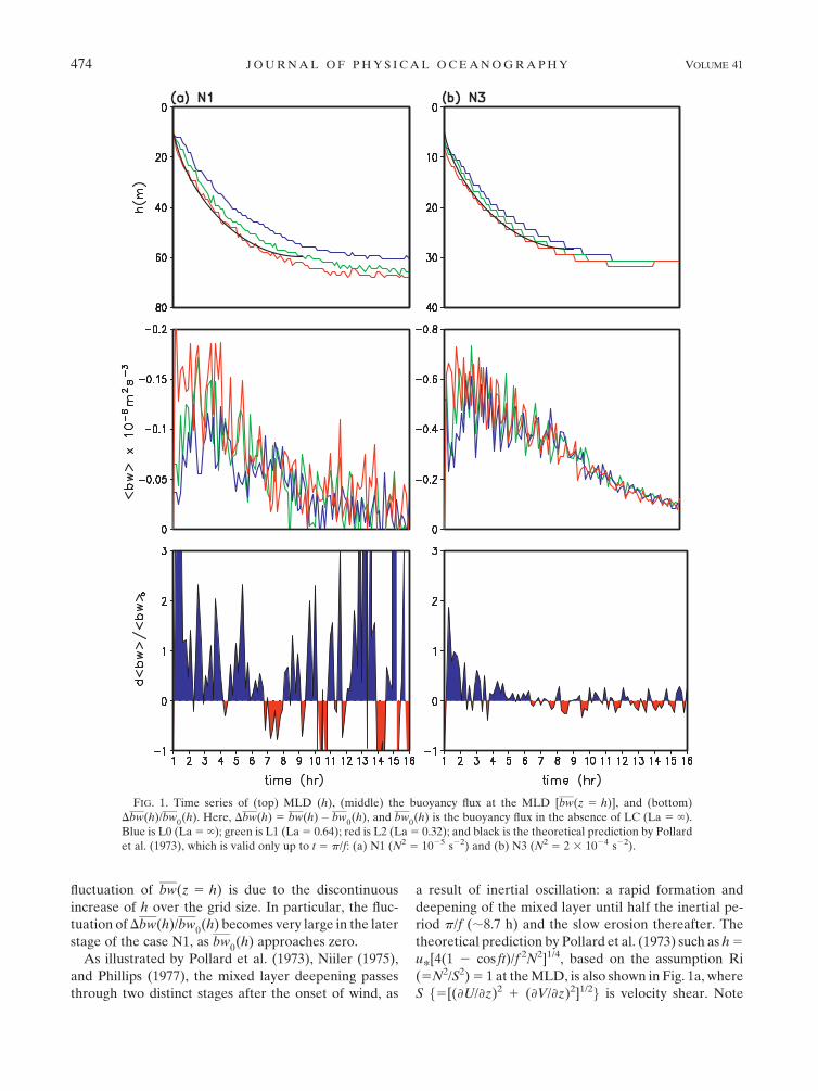
fluctuation of bw(z 5 h) is due to the discontinuous
increase of h over the grid size. In particular, the fluc-
tuation of Dbw(h)/bw0(h) becomes very large in the later
stage of the case N1, as bw0(h) approaches zero.
As illustrated by Pollard et al. (1973), Niiler (1975),
and Phillips (1977), the mixed layer deepening passes
through two distinct stages after the onset of wind, as
a result of inertial oscillation: a rapid formation and
deepening of the mixed layer until half the inertial pe-
riod p/f (;8.7 h) and the slow erosion thereafter. The
theoretical prediction by Pollard et al. (1973) such as h 5
u*[4(1 2 cos ft)/f 2N2]1/4, based on the assumption Ri
(5N2/S2) 5 1 at the MLD, is also shown in Fig. 1a, where
S f5[(›U/›z)2 1 (›V/›z)2]1/2g is velocity shear. Note
FIG. 1. Time series of (top) MLD (h), (middle) the buoyancy flux at the MLD [bw(z 5 h)], and (bottom)
Dbw(h)/bw0(h). Here, Dbw(h) 5 bw(h)� bw
0(h), and bw
0(h) is the buoyancy flux in the absence of LC (La 5 ‘).
Blue is L0 (La 5 ‘); green is L1 (La 5 0.64); red is L2 (La 5 0.32); and black is the theoretical prediction by Pollard
et al. (1973), which is valid only up to t 5 p/f: (a) N1 (N2 5 1025 s22) and (b) N3 (N2 5 2 3 1024 s22).
474 J O U R N A L O F P H Y S I C A L O C E A N O G R A P H Y VOLUME 41
that the Pollard et al.’s prediction is valid only up to t 5
p/f. It is interesting that a better agreement is found
between LES results and the Pollard’s prediction, when
LC is stronger (L2). It may be related to the fact that
more uniform temperature and velocity profiles are
generated under stronger LC, which is consistent with
the hypothesis used in Pollard’s model.
Langmuir circulation is found to enhance the mixed
layer deepening in general. However, the most remark-
able feature in Fig. 1 is that the effect of LC, represented
by Dbw(h)/bw0(h), is stronger when h is shallower in the
initial stage and when stratification is weaker, as in the
case N1. On the other hand, the effect of LC is negligible
when stratification is strong and MLD is deep, as in the
later stage of N3.
b. Variation of entrainment with LC
The factors to determine the entrainment rate we
(5dh/dt) in the presence of LC can be represented as
we5 f (h, DB, u*, U
s, l, f ). (1)
Dimensional analysis leads to
we
u*5 f
hDB
u2*
,hDB
y2L
,h
l,
h
u*/f
!, (2)
where yL [5(Usu*2)1/3] and hDB/yL
2 [5(hDB/u*2)(u*/yL)2]
are used instead of Us and yL/u*. The momentum dif-
ference across MLD [(DU)2 1 (DV)2]1/2 cannot be an
independent parameter, because it is determined by u*,
h, N, and f, as long as momentum is generated by wind
stress.
If h/l and h/(u*/f) remain invariant, we assume the
functional form of (2) as we/u* 5 f1(hDB/u*2)[1 1
f2(hDB/yL2)], where f2 approaches zero with the increase
of hDB/yL2. In this case, the difference of we between the
cases with and without LC Dwe or equivalently Dbw(h)
(5DweDB) can be expressed as
Dbw(h)
bw(h)0
5 f2
hDB
y 2L
� �. (3)
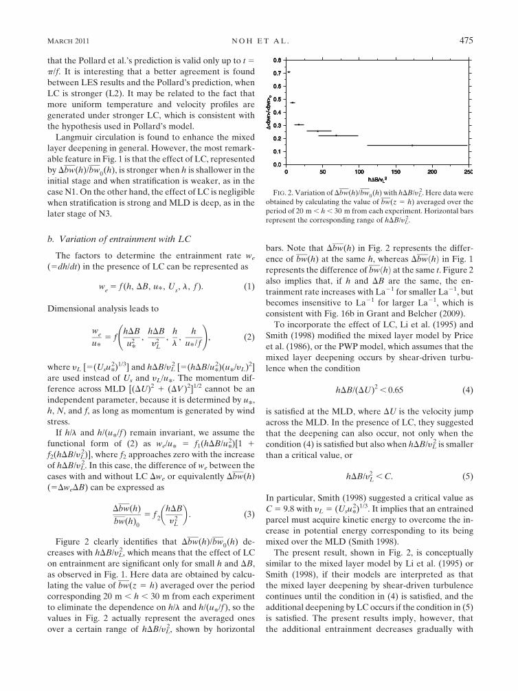
Figure 2 clearly identifies that Dbw(h)/bw0(h) de-
creases with hDB/yL2, which means that the effect of LC
on entrainment are significant only for small h and DB,
as observed in Fig. 1. Here data are obtained by calcu-
lating the value of bw(z 5 h) averaged over the period
corresponding 20 m , h , 30 m from each experiment
to eliminate the dependence on h/l and h/(u*/f), so the
values in Fig. 2 actually represent the averaged ones
over a certain range of hDB/yL2, shown by horizontal
bars. Note that Dbw(h) in Fig. 2 represents the differ-
ence of bw(h) at the same h, whereas DbwðhÞ in Fig. 1
represents the difference of bwðhÞ at the same t. Figure 2
also implies that, if h and DB are the same, the en-
trainment rate increases with La21 for smaller La21, but
becomes insensitive to La21 for larger La21, which is
consistent with Fig. 16b in Grant and Belcher (2009).
To incorporate the effect of LC, Li et al. (1995) and
Smith (1998) modified the mixed layer model by Price
et al. (1986), or the PWP model, which assumes that the
mixed layer deepening occurs by shear-driven turbu-
lence when the condition
hDB/(DU)2, 0.65 (4)
is satisfied at the MLD, where DU is the velocity jump
across the MLD. In the presence of LC, they suggested
that the deepening can also occur, not only when the
condition (4) is satisfied but also when hDB/yL2 is smaller
than a critical value, or
hDB/y2L , C. (5)
In particular, Smith (1998) suggested a critical value as
C 5 9.8 with yL 5 (Usu*2)1/3. It implies that an entrained
parcel must acquire kinetic energy to overcome the in-
crease in potential energy corresponding to its being
mixed over the MLD (Smith 1998).
The present result, shown in Fig. 2, is conceptually
similar to the mixed layer model by Li et al. (1995) or
Smith (1998), if their models are interpreted as that
the mixed layer deepening by shear-driven turbulence
continues until the condition in (4) is satisfied, and the
additional deepening by LC occurs if the condition in (5)
is satisfied. The present results imply, however, that
the additional entrainment decreases gradually with
FIG. 2. Variation of Dbw(h)/bw0(h) with hDB/yL2. Here data were
obtained by calculating the value of bw(z 5 h) averaged over the
period of 20 m , h , 30 m from each experiment. Horizontal bars
represent the corresponding range of hDB/yL2.
MARCH 2011 N O H E T A L . 475

hDB/yL2 rather than disappears abruptly at a critical
value of hDB/yL2. The criterion hDB/yL
2 , 9.8, suggested
by Smith (1998), roughly represents the regime of the
significant effect of LC in Fig. 2.
The present result is also consistent with the previous
reports that the effect of LC is mostly confined to the
initial stages of mixed layer growth, and there is no ev-
idence that LC has a direct role in mixing near the base
of a 40–60-m-deep mixed layer (Weller and Price 1988;
Skyllingstad et al. 2000; Thorpe 2004). The LES results
(Sullivan et al. 2007; Grant and Belcher 2009; Kukulka
et al. 2009), in which LC induces a noticeable increase of
entrainment, were obtained under the condition in
which hDB/yL2 is less than 40. Note that these simulations
started with the initial profiles with DT 5 08C, h0 larger
than 30 m, and weak stratification below (e.g., ›T/›z 5
0.01 K m21).
c. Modification of profiles in the mixedlayer under LC
Here we investigate how the profiles of various phys-
ical quantities in the mixed layer, such as velocity shear,
stratification, eddy viscosity and diffusivity, and the ve-
locity and length scales of turbulence, are modified under
FIG. 3. Profiles of velocity shear S2 and stratification N2 [dotted line is L0 (La 5 ‘), dashed line is L1 (La 5 0.64), and
solid line is L2 (La 5 0.32)]: (a) N1 (t 5 2 h) and (b) N3 (t 5 15 h).
476 J O U R N A L O F P H Y S I C A L O C E A N O G R A P H Y VOLUME 41

the influence of LC, which helps to clarify the mechanism
for the enhanced entrainment under LC. Profiles are
made at t 5 2 h for the case N1 and at t 5 15 h for the case
N3, which represent the typical cases of strong and weak
effects, respectively, of LC on the mixed layer deepening,
as mentioned in previous sections.
The values of S2 are drastically decreased in the
presence of LC in both cases of N1 and N3, as already
reported in previous reports (McWilliams et al. 1997;
Noh et al. 2004; Li et al. 2005; Skyllingstad 2005) (Fig. 3).
Especially in the case of L2, S2 almost disappears at
a certain depth (z/h ; 0.2), suggesting that momen-
tum transport may occur by means of nonlocal mixing
(McWilliams and Sullivan 2000; Smyth et al. 2002).
Furthermore, Fig. 3 shows that S2 decreases at the MLD
as well as within the mixed layer. It should be men-
tioned, however, that the magnitude of shear production
at the MLD is nearly the same, regardless of LC (not
shown). The values of N2 also decrease in the presence
of LC, especially in the case of N1, but they are not so
sensitive to the presence of LC as S2. Generally speak-
ing, LC always enhances vertical mixing greatly within
the mixed layer, regardless of whether the contribution
of LC to the mixed layer deepening is significant.
As expected from the fact that LC is more effective to
reduce S2 than N2, Ri (5N2/S2) becomes larger under
LC within the mixed layer (Fig. 4). It is also found that
the decrease of Ri is less sensitive near the MLD than
FIG. 4. (top) Profiles of Ri and (bottom) time series of Ri (z 5 h) [dotted line is L0 (La 5 ‘), dashed line is L1
(La 5 0.64), and solid line is L2 (La 5 0.32)]: (a) N1 (t 5 2 h) and (b) N3 (t 5 15 h).
MARCH 2011 N O H E T A L . 477

within the mixed layer. The time series of Ri (z 5 h)
shows that Ri maintains a constant value at the MLD up
to t ; p/f after the initial stage: that is, Ri (z 5 h) ; 0.8,
which is consistent with the assumption made in Pollard
et al. (1973) [Ri (z 5 h) 5 1]. After the inertial period
(t . p/f ), however, it increases exponentially with time,
as the mean velocity within the mixed layer decreases
a result of inertial oscillation, as shown by Noh et al.
(2010).
It is possible to consider that the increased entrain-
ment under LC is attributed to the enhanced shear at the
MLD resulting from the stronger mixing of momentum
by LC within the mixed layer, as mentioned in Thorpe
(2004). The decrease of S2 (z 5 h) in the presence of LC
suggests, however, that it is more likely to be attributed
to the direct effect of engulfment by large-scale eddies of
LC impinging on the MLD, similarly to the case of
convective eddies.
In accordance with the enhanced vertical mixing
within the mixed layer, much larger eddy viscosity and
diffusivity, Km and Kh, are found in the presence of
LC, in both N1 and N3 (Fig. 5). Here Km and Kh are
calculated by �uw›U/›z� yw›V/›z 5 Km[(›U/›z)21
(›V/›z)2] and �bw 5 Kh›B/›z. Note that negative Km
FIG. 5. Profiles of eddy viscosity Km and eddy diffusivity Kh [dotted line is L0 (La 5 ‘), dashed line is L1 (La 5 0.64),
and solid line is L2 (La 5 0.32)]: (a) N1 (t 5 2 h) and (b) N3 (t 5 15 h).
478 J O U R N A L O F P H Y S I C A L O C E A N O G R A P H Y VOLUME 41

appears near the surface at L2, as observed by Sullivan
et al. (2007), reflecting the nonlocal nature of vertical
mixing by LC.
The profiles of velocity and length scales of turbu-
lence, q [5(uiui)1/2] and l, indicate that the increase of
Km and Kh under LC is attributed predominantly to the
increase of l, although both q and l increase under LC
(Fig. 6). Here, l is calculated from Kh 5 Shql with Sh 5
0.49 (Mellor and Yamada 1982; Noh and Kim 1999). It
indicates that the increase of TKE itself is not sufficient
to explain the stronger vertical mixing under LC. It is
also interesting to find that the ratio of l between the
cases with and without LC is much larger than 1 when N2
is small, such as at z/h ; 0.2, but it is close to 1 when N2
becomes large, such as at z/h ; 0.8. This will be dis-
cussed further in the next section.
d. Parameterization of vertical mixing inthe presence of LC
The suppression of vertical mixing under stratification
is often parameterized in terms of Ri (5N2/S2) in mixed
layer models (Pacanowski and Philander 1981; Mellor
FIG. 6. Profiles of the mixing length scale l and the turbulent velocity scale q. Here, l was calculated from Kh 5 Shql
with Sh 5 0.49 [dotted line is L0 (La 5 ‘), dashed line is L1 (La 5 0.64), and solid line is L2 (La 5 0.32)]: (a) N1 (t 5
2 h) and (b) N3 (t 5 15 h).
MARCH 2011 N O H E T A L . 479
and Yamada 1982; Kantha and Clayson 1994; Canuto
et al. 2001). It implies that, as in the case of the atmo-
spheric boundary layer, entrainment is dominantly
contributed by turbulent eddies generated by velocity
shear. This type of parameterization is usually evaluated
based on the assumption of local equilibrium Ps 1 Pb 5 «
with the neglect of TKE flux, where Ps is shear pro-
duction, Pb is buoyancy production/decay, and « is dis-
sipation rate (Mellor and Yamada 1982; Kantha and
Clayson 1994; Canuto et al. 2001). It has been found,
however, that the divergence of TKE flux becomes a
dominant turbulence source in the presence of LC (Noh
et al. 2004; Sullivan et al. 2007; Polton and Belcher 2007;
Grant and Belcher 2009).
Noh and Kim (1999) suggested that the parameteriza-
tion of stratification on vertical mixing in the ocean mixed
layer should be parameterized in terms of the Richardson
number based on TKE itself fi.e., Rt [5(Nl0/q)2], rather
than Rig, because shear production is no longer a domi-
nant source of TKE. Here, l0 is the length scale in the
homogeneous mixed layer. In particular, they suggested
a formula such as
l/l0
5 (1 1 aRt)�1/2 (6)
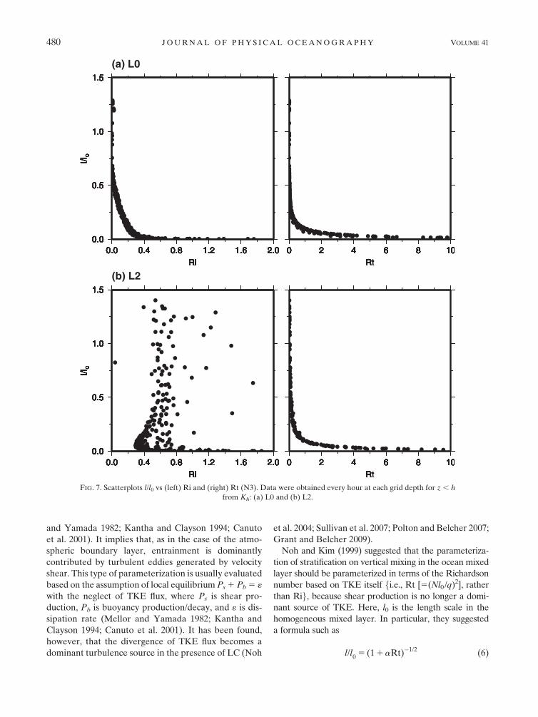
FIG. 7. Scatterplots l/l0 vs (left) Ri and (right) Rt (N3). Data were obtained every hour at each grid depth for z , h
from Kh: (a) L0 and (b) L2.
480 J O U R N A L O F P H Y S I C A L O C E A N O G R A P H Y VOLUME 41

with an empirical constant a, based on the assumption
that l approaches the buoyancy length scale lb (5q/N)
with increasing stratification. Here, the length scale l0 is
prescribed by an empirical formula as
1
l0
51
k(z 1 z0)
11
h, (7)
where k is the von Karman constant (50.4) and the
length scale at the sea surface is given by z0 5 1 m (Noh
and Kim 1999). The mixed layer model based on this
parameterization is shown to reproduce well the realistic
upper-ocean structure (Noh and Kim 1999; Noh et al.
2002, 2005, 2007; Hasumi and Emori 2004; Rascle and
Ardhuin 2009).
Figure 7 examines how l/l0 varies with Ri and Rt for
the case of N3 with and without LC (L2-N3 and L0-N3).
The data were obtained every hour at each grid depth
from the surface to MLD. The data l/l0 versus Ri show
a good collapse in the absence of LC, but they show
a large scatter without apparent correlation in the
presence of LC. It indicates that Ri is an appropriate
parameter only in the case where shear production is
a dominant source of TKE as in the atmospheric
boundary layer. On the other hand, the data l/l0 versus
Rt show a good collapse in both cases with and without
LC. Moreover, the functional forms of correlation are
similar to each other, suggesting the universality of the
parameterization in terms of Rt. Figure 7 convinces us
that vertical mixing should be parameterized in terms of
Rt instead of Ri in the ocean mixed layer.
To clarify further the relationship between l/l0 and Rt,
we plot the data from six experiments (L0-N1, L1-N1,
L2-N1, L0-N3, L1-N3, and L2-N3) in the logarithmic
scale for both Km and Kh (Fig. 8). To calculate l/l0 for
Km, Km 5 Smql is used with Sm 5 0.39 (Mellor and
Yamada 1982; Noh and Kim 1999), and the data with
negative l/l0, originating from the negative Km near the
surface in the case L2 (Fig. 4), are not included. The
general pattern is similar for Km and Kh, although data
are slightly more scattered for Km.
It is remarkable to find that the data l/l0 versus Rt
more or less collapse at larger Rt (Rt . ;1), regardless
of the presence of LC, as the similarity in the relation-
ship between l/l0 and Rt in Fig. 7 suggests. In particular,
the relationship between l/l0 and Rt is found to follow
(6) with a ; 50, as shown by a solid line. The slope
corresponding to l/l0 } Rt21/2 indicates that l approaches
a21/2lb with increasing Rt.
Meanwhile, Fig. 8 also shows that, at smaller Rt (Rt ,
;1), l/l0 becomes larger in the case with LC than without
LC, and the ratio of l/l0 between the cases with and
without LC continues to increase to above 10 with the
decrease of Rt. The ratio is larger for stronger LC. Note
also that l increases by more than 10 times in the pres-
ence of LC, when N2 almost disappears at z ; 0.2h, but it
is less affected by LC, when N2 becomes larger at z ;
0.8h in Fig. 6. This confirms again the fact that the in-
fluence of LC on the mixed layer deepening is important
only for weaker stratification and shallower depth, as
already found in Figs. 1 and 2.
The general pattern for l/l0 versus Rt, shown in Fig. 8,
can be explained in terms of the increase of l0 under LC.
Equation (6) predicts that l approaches l0, as Rt ap-
proaches 0, whereas it approaches a21/2lb independent of
l0, as Rt becomes large. Because the length scale in the
presence of LC is much larger than the one given by (7),
l/l0 becomes much larger than 1 in Fig. 8 as Rt approaches
0. Consequently, we expect that the parameterization (6)
remains valid, regardless of the presence of LC, but
a much larger value of l0 should be used in the presence of
LC. For example, if l0 is replaced by gl0, (6) is modified to
l/l0
5 g(1 1 ag2Rt)�1/2. (8)
The prediction from (8) with g 5 10 is shown to predict
well the relationship between l/l0 and Rt for the case L2
FIG. 8. Scatterplots in the logarithmic scale for l/l0 vs Rt. Data
were obtained every hour at each grid depth for z , h [blue (N1,
L0), light blue (N3, L0), green (N1, L1), light green (N3, L1), red
(N1, L2), and light red (N3, L2)]. The black solid and dashed lines
represent the predictions from l/l0 5 (1 1 aRt)21/2 and l/l0 5 g(1 1
ag2Rt)21/2, where a 5 50 and g 5 10: (a) Km and (b) Kh.
MARCH 2011 N O H E T A L . 481

(Fig. 7). The length scale in the presence of LC may
depend on l and h as well as La, however.
e. Sensitivity to the e-folding depth ofthe Stokes drift
It has been reported from the recent LES works that
the vertical TKE can be affected by the e-folding depth
of the Stokes drift, or l, when l/h is large (Harcourt and
D’Asaro 2008; Grant and Belcher 2009). To investigate
the sensitivity of l to the mixed layer deepening, we
compared the results with l 5 40 and 80 m for the case
L2. Figure 9 shows that the effect of l is insignificant in
both N1 and N3, although the mixed layer deepening is
slightly faster for larger l in the initial stage.
4. Conclusions
Analysis of LES data reveals the consistent pattern
with regard to the influence of LC on the mixed layer
deepening in the present paper. That is, LC induces
a significant enhancement of the mixed layer deepening
only if h and DB are small. This property is attested by
the facts that the difference of the entrainment at the
MLD between the cases with and without LC decreases
with hDB/yL2 (Fig. 2) and that the ratio of the mixing
length scale l between the cases with and without LC is
close to 1 for larger Rt (Rt . ;1) but continues to in-
crease to above 10 with the decrease of Rt (Fig. 8). The
present result is in agreement with previous reports that
the effect of LC is mostly confined to the initial stage of
mixed layer growth (Weller and Price 1988; Skyllingstad
et al. 2000; Thorpe 2004). It is also conceptually similar
to the model suggested by Li et al. (1995) and Smith
(2001) that the additional deepening of the mixed layer
occurs in the presence of LC, when hDB/yL2 becomes less
than a critical value.
The magnitude of velocity shear at the MLD tends to
be slightly decreased in the presence of LC (Fig. 3). It
suggests that the engulfment by large-scale eddies of LC
impinging on the density interface at the MLD may
contribute to the increased entrainment directly, simi-
larly to convective eddies, rather than the increased
shear at the MLD. However, unlike convective eddies,
which is driven continuously by buoyancy force, eddies
generated by LC are essentially unforced and behave
inertially, because the vortex force is confined to near
the surface. Therefore, it is expected that eddies generated
FIG. 9. Time series of (top) MLD (h) and (bottom) the buoyancy flux at the MLD [bw(z 5 h)] for the case L2 (solid
line is l 5 40 m and dashed line is l 5 80 m): (a) N1 and (b) N3.
482 J O U R N A L O F P H Y S I C A L O C E A N O G R A P H Y VOLUME 41

by LC are efficient for the vertical mixing under weak
stratification, such as within the mixed layer or across
the MLD with small DB, but their contribution to the
vertical mixing becomes negligible under strong strati-
fication, such as across the MLD with large DB. More-
over, the effect of LC decreases with depth, because the
intensity of eddies generated by LC decreases rapidly
with depth, unlike convective eddies.
Furthermore, it is clearly illustrated that the effect of
stratification on vertical mixing in the presence of LC
should be parameterized in terms of Rt [5(Nl0/q)2] in-
stead of Ri [5(N/S)2], because shear production is not
a dominant source of TKE any more. In particular, the
mixing length scale is parameterized by l/l0 5 (1 1
aRt)21/2 with a ; 50, as suggested by Noh and Kim
(1999), regardless of the presence of LC. However, the
presence of LC makes l0 much larger than convention-
ally used for the boundary layer. The inclusion of non-
local mixing may be necessary for the more elaborate
parameterization of vertical mixing, especially to ac-
count for negative Km near the surface at small La (Fig.
5), but the present result suggests that the effect of LC
can be largely represented by the increase of the mixing
length scale. It is also found that the increase of Km and
Kh under LC is attributed predominantly to the increase
of l, although both q and l increase under LC.
Finally, it is important to mention that the present
simulation is initiated by applying the wind stress to
a motionless mixed layer with stratification, which is
more relevant to storm events. However, most analyses
are performed after quasi-equilibrium state is reached at
about 10h0/u* (;1 h) after the onset of the wind stress,
which implies that the present result can be applied
more generally.
Acknowledgments. This work was supported by the
National Research Foundation of Korea Grant funded by
the Korean Government (MEST) (NRF-2009-C1AAA001-
0093068), by the Korean Ocean Research and Develop-
ment Institute (KORDI) research program PE98512, and
by the project ‘‘Research for the Meteorological Obser-
vation Technology and Its Application’’ at the National
Institute of Meteorological Research.
REFERENCES
Ayotte, K. W., and Coauthors, 1996: An evaluation of neutral and
convective planetary boundary-layer parameterizations relative
to large eddy simulations. Bound.-Layer Meteor., 79, 131–175.
Canuto, V. M., A. Howard, Y. Cheng, and M. S. Dubovikov, 2001:
Ocean turbulence. Part I: One-point closure model—
Momentum and heat vertical diffusivities. J. Phys. Oceanogr.,
31, 1413–1426.
Craik, A. D. D., and S. Leibovich, 1976: A rational model for
Langmuir circulations. J. Fluid Mech., 73, 401–426.
D’Alessio, J. S. D., K. Abdella, and N. A. McFarlane, 1998: A new
second-order turbulence closure scheme for modeling the
ocean mixed layer. J. Phys. Oceanogr., 28, 1624–1641.
D’Asaro, E. A., and G. T. Dairiki, 1997: Turbulence intensity
measurements in a wind-driven mixed layer. J. Phys. Ocean-
ogr., 27, 2009–2022.
Gargett, A. E., and J. R. Wells, 2007: Langmuir turbulence in
shallow water. Part 1. Observations. J. Fluid Mech., 576, 27–61.
Gerbi, G. P., J. H. Trowbridge, E. A. Terray, A. J. Pleuddemann,
and T. Kukulka, 2009: Observation of turbulence in the ocean
surface boundary layer: Energetics and transport. J. Phys.
Oceanogr., 39, 1077–1096.
Grant, A. L. M., and S. E. Belcher, 2009: Characteristics of Lang-
muir turbulence in the ocean mixed layer. J. Phys. Oceanogr.,
39, 1871–1887.
Harcourt, R. R., and E. A. D’Asaro, 2008: Large-eddy simulation
of Langmuir turbulence in pure wind seas. J. Phys. Oceanogr.,
38, 1542–1562.
Hasumi, H., and S. Emori, 2004: Coupled GCM (MIROC) de-
scription. K-1 Tech. Rep. 1, 39 pp.
Kantha, L. H., and C. A. Clayson, 1994: An improved mixed layer
model for geophysical applications. J. Geophys. Res., 99,
25 235–25 266.
——, and ——, 2004: On the effect of surface gravity waves on
mixing in the ocean mixed layer. Ocean Modell., 6, 101–124.
Kukulka, T., A. J. Plueddemann, J. H. Trowbridge, and P. P. Sullivan,
2009: Significance of Langmuir circulation in upper mixing:
Comparison of observations and simulations. Geophys. Res.
Lett., 36, L10603, doi:10.1029/2009GL037620.
Leibovich, S., 1983: The form and dynamics of Langmuir circula-
tion. Annu. Rev. Fluid Mech., 15, 391–427.
Li, M., and C. Garrett, 1997: Mixed layer deepening due to Lang-
muir circulation. J. Phys. Oceanogr., 27, 121–132.
——, K. Zahariev, and C. Garrett, 1995: Role of Langmuir circu-
lation in the deepening of the ocean surface mixed layer.
Science, 270, 1955–1957.
——, C. Garrett, and E. Skyllingstad, 2005: A regime diagram for
classifying large eddies in the upper ocean. Deep-Sea Res. I, 52,
259–278.
McWilliams, J. C., and P. P. Sullivan, 2000: Vertical mixing by
Langmuir circulation. Spill Sci. Technol. Bull., 6, 225–237.
——, ——, and C. H. Moeng, 1997: Langmuir turbulence in the
ocean. J. Fluid Mech., 334, 1–30.
Mellor, G. L., and T. Yamada, 1982: Development of a turbulent
closure model for geophysical fluid problems. Rev. Geophys.
Space Phys., 20, 851–875.
Min, H. S., and Y. Noh, 2004: Influence of the surface heating on
Langmuir circulation. J. Phys. Oceanogr., 34, 2630–2641.
Niiler, P. P., 1975: Deepening of the wind-mixed layer. J. Mar. Res.,
33, 405–422.
Noh, Y., and H. J. Kim, 1999: Simulations of temperature and turbu-
lence structure of the oceanic boundary layer with the improved
near-surface process. J. Geophys. Res., 104, 15 621–15 634.
——, and S. Nakada, 2010: Examination of the particle flux from
the convective mixed layer by large eddy simulation. J. Geo-
phys. Res., 115, C05007, doi:10.1029/2009JC005669.
——, C. J. Jang, T. Yamagata, P. C. Chu, and C. H. Kim, 2002:
Simulation of more realistic upper ocean process from an
OGCM with a new ocean mixed layer model. J. Phys. Oceanogr.,
32, 1284–1307.
——, H. S. Min, and S. Raasch, 2004: Large eddy simulation of the
ocean mixed layer: The effects of wave breaking and Lang-
muir circulation. J. Phys. Oceanogr., 34, 720–735.
MARCH 2011 N O H E T A L . 483

——, Y. J. Kang, T. Matsuura, and S. Iizuka, 2005: Effect of the
Prandtl number in the parameterization of vertical mixing in
an OGCM of the tropical Pacific. Geophys. Res. Lett., 32,
L23609, doi:10.1029/2005GL024540.
——, I. S. Kang, M. Herold, and S. Raasch, 2006: Large eddy
simulation of particle settling in the ocean mixed layer. Phys.
Fluids, 18, 085109, doi:10.1063/1.2337098.
——, B. Y. Yim, S. H. You, J. H. Yoon, and B. Qiu, 2007: Seasonal
variation of eddy kinetic energy of the North Pacific Subtropical
Countercurrent simulated by an eddy-resolving OGCM. Geo-
phys. Res. Lett., 34, L07601, doi:10.1029/2006GL029130.
——, G. Goh, S. Raasch, and M. Gryschka, 2009: Formation of
a diurnal thermocline in the ocean mixed layer simulated by
LES. J. Phys. Oceanogr., 39, 1244–1257.
——, ——, and ——, 2010: Examination of the mixed layer deep-
ening process during convection using LES. J. Phys. Ocean-
ogr., 40, 2189–2195.
Pacanowski, R. C., and S. G. H. Philander, 1981: Parameterization
of vertical mixing in numerical models. J. Phys. Oceanogr., 11,1443–1451.
Phillips, O. M., 1977: The Dynamics of the Upper Ocean. Cam-
bridge University Press, 295–308.
Plueddemann, A., J. A. Smith, D. M. Farmer, R. A. Weller,
W. R. Crawford, R. Pinkel, S. Vagle, and A. Gnanadesikan,
1996: Structure and variability of Langmuir circulation during
the Surface Waves Processes Program. J. Geophys. Res., 101,3525–3543.
Pollard, R. T., P. B. Rhines, and R. O. R. Y. Thompson, 1973: The
deepening of the wind-mixed layer. J. Geophys. Fluid Dyn., 3,
381–404.
Polton, J. A., and S. E. Belcher, 2007: Langmuir turbulence and
deeply penetrating jets in an unstratified mixed layer. J. Geo-
phys. Res., 112, C09020, doi:10.1029/2007JC004205.
Price, J. F., R. A. Weller, and R. Pinkel, 1986: Diurnal cycles of
current, temperature and turbulent diffusion in a model of the
equatorial upper ocean. J. Geophys. Res., 91, 8411–8427.
Raasch, S., and M. Schroter, 2001: A large eddy simulation model
performing on massively parallel computers. Meteor. Z., 10,
363–372.
Rascle, N., and F. Ardhuin, 2009: Drift and mixing under the ocean
surface revisited: Stratified conditions and model-data compar-
isons. J. Geophys. Res., 114, C02016, doi:10.1029/2007JC004466.
Skyllingstad, E. D., 2001: Scales of Langmuir circulation generated
using a large-eddy simulation model. Spill Sci. Technol. Bull.,
6, 239–246.
——, 2005: Langmuir circulation. Marine Turbulence, H. Z. Baumert,
J. H. Simpson, and J. Sundermann, Eds., Cambridge University
Press, 277–282.
——, and D. W. Denbo, 1995: An ocean large-eddy simulation of
Langmuir circulations and convection in the surface mixed
layer. J. Geophys. Res., 100, 8501–8522.
——, W. D. Smith, and G. B. Crawford, 2000: Resonant wind-
driven mixing in the ocean boundary layer. J. Phys. Oceanogr.,
30, 1866–1890.
Smith, J. A., 1992: Observed growth of Langmuir circulation. J. Geo-
phys. Res., 97, 5651–5667.
——, 1998: Evolution of Langmuir circulation during a storm. J. Geo-
phys. Res., 103, 12 649–12 668.
——, 2001: Observations and theories of Langmuir circulation: A
story of mixing. Fluid Mechanics and the Environment: Dy-
namical Approaches, J. L. Lumley, Ed., Springer, 295–314.
Smyth, W. D., E. D. Skyllingstad, G. B. Crawford, and H. Wijesekera,
2002: Nonlocal fluxes and Stokes drift effects in the K-profile
parameterization. Ocean Dyn., 52, 104–115.
Sullivan, P. P., J. C. McWilliams, and W. K. Melville, 2007: Surface
gravity wave effects in the oceanic boundary layer: Large-eddy
simulation with vortex force and stochastic breakers. J. Fluid
Mech., 593, 405–452.
Tejada-Martınez, A. E., and C. E. Grosch, 2007: Langmuir turbu-
lence in shallow water. Part 2. Lange-eddy simulation. J. Fluid
Mech., 576, 63–108.
Thorpe, S. A., 2004: Langmuir circulation. Annu. Rev. Fluid Mech.,
36, 55–79.
——, T. R. Osborn, J. F. E. Jackson, A. J. Hall, and R. G. Lueck,
2003: Measurements of turbulence in the upper ocean mixing
layer using Autosub. J. Phys. Oceanogr., 33, 122–145.
Weller, R. A., and J. F. Price, 1988: Langmuir circulation within the
oceanic mixed layer. Deep-Sea Res., 35, 711–747.
484 J O U R N A L O F P H Y S I C A L O C E A N O G R A P H Y VOLUME 41


