
American Institute of Aeronautics and Astronautics
1
Investigating Aeroelastic Performance of Multi-MegaWatt
Wind Turbine Rotors Using CFD
David A. Corson1
Altair Engineering, Inc., Clifton Park, NY, 12065
D. Todd Griffith2
Sandia National Laboratories, Albuquerque, NM, 87185
Tom Ashwill3
Sandia National Laboratories, Albuquerque, NM, 87185
Farzin Shakib4
Altair Engineering, Inc., Mountain View, CA, 94043
Recent trends in wind power technology are focusing on increasing power output
through an increase in rotor diameter. As the rotor diameter increases, aeroelastic effects
become increasingly important in the design of an efficient blade. A detailed understanding
of the fluid elastic coupling can lead to improved designs; yielding more power, reduced
maintenance, and ultimately leading to an overall reduction in the cost of electricity. In this
work, a high fidelity Computational Fluid Dynamics (CFD) methodology is presented for
performing fully coupled Fluid-Structure Interaction (FSI) simulations of wind turbine
blades and rotors using a commercially available flow solver, AcuSolve. We demonstrate the
technique using a 13.2 MW blade design.
I. Introduction
recent report published by the Department of Energy (DOE) has concluded that the United States possesses
sufficient wind resources to harvest 20% of its energy requirements through wind turbine power production.
Achieving this goal requires close collaboration between government laboratories, academic institutions, and
industrial partners in the wind power community. The majority of recent installations of utility-scale wind turbines
utilize a horizontal axis, terrestrial mounted, 3-bladed rotor design having a power output ranging from 1.5 to 2.5
MW. Typical rotor diameters for these installations range between 80 and 100 meters. However, as the industry
looks to increase the amount of power extracted from the wind, alternate rotor designs are being pursued. Sandia National Laboratories is currently embarking on a study of large blades intended to produce higher power rotors.
This work follows many years of research on structural mechanics innovations for improved blade technology in the
development of Sandia 9-m research blades. The philosophy behind Sandia’s current design effort is to provide the
industry with a 100-meter reference blade design for a 13.2 MW rotor1. A major consequence of increasing the
blade length in this fashion is the increased importance of the aeroelastic effects on the blade. Accompanying the
longer blade lengths is the potential for significant deflections of the structure due to both aerodynamic and
gravitational forces. Accompanying this is the possibility for the blade to experience flutter, a phenomena involving
the interaction of the fluid and structural frequencies to produce large amplitude, periodic motion. An important step
in the design of such large turbine blades is the incorporation of an analysis technique that can provide engineers
1 AcuSolve Program Manager, 58 Clifton Country Rd., Ste 106, Clifton Park, NY 2 Senior Member of the Technical Staff, Analytical Structural Dynamics Dept., Senior Member AIAA. 3 Analytical Structural Dynamics Dept. 4 Vice President – CFD Technology, 2685 Marine Way, Ste 1421, Mountain View, CA
A
53rd AIAA/ASME/ASCE/AHS/ASC Structures, Structural Dynamics and Materials Conference<BR>20th AI23 - 26 April 2012, Honolulu, Hawaii
AIAA 2012-1827
Copyright © 2012 by the American Institute of Aeronautics and Astronautics, Inc. All rights reserved.

American Institute of Aeronautics and Astronautics
2
with detailed information on the fully coupled aeroelastic behavior of the blades. Current wind turbine design
practices look towards desktop engineering tools such as FAST2 and ADAMS3 to provide information about the
aero-elastic behavior of the turbines. Additionally, frequency based approaches, such as those of Lobitz are also
used18
. Each of these techniques has advantages and disadvantages. Unfortunately, no largely agreed upon method
for evaluating aeroelastic performance has been identified. The industry will certainly benefit from a more
fundamental technique for situations where there is large scale disagreement regarding the aeroelastic performance of a blade among the aforementioned methods. There is also need for a higher fidelity tool for further investigating
designs in which the previously mentioned tools reveal little or no margin on aeroelastic performance.
Implicit within the existing aeroelastic predictive tools are a number of assumptions that introduce uncertainty
into the prediction of the aeroelastic coupling of the blades. On the aerodynamics side, the Aerodyn4 code provides
the aerodynamic load computation for both FAST and ADAMS. Lobitz18 illustrated as much as a 30% difference in
the prediction of flutter speed when using ADAMS and AERODYN to investigate the aeroelastic stability of a wind
turbine blade. The differences were due solely to the selection of different aerodynamic options within AERODYN.
Resor and Paquette19 also find sensitivity to their predictions when applying a frequency based method to determine
the flutter speed. This sensitivity resulted from the technique used to determine the equivalent beam properties of a
blade. The primary aim of this work is to address all of these limitations with a general purpose, high-fidelity, fully
coupled aerodynamic and structural representation of the rotor. The need for such technology becomes increasingly
important as the industry continues to push the envelope on advanced designs to exploit complex phenomena such as bend-twist coupling for passive load control. A fundamentally based, general purpose aeroelastic modeling
approach will allow the investigation of structural and aerodynamic performance for off-axis loading cases, active
control structures, and many more design cases not handled by modern tools. Sandia’s 100-m reference model was
chosen specifically for this work due to its large scale and complex fluid/elastic coupling. In particular, blade
deflection and aeroelastic stability are the performance quantities that will be a focus of this work.
An evolving approach for generating performance data on wind turbine rotors is through the use of
Computational Fluid Dynamics (CFD). In addition to performing detailed flow field predictions around the rotor,
modern CFD codes are increasingly capable of performing multiphysics simulations. These capabilities include the
ability to run aeroelastic simulations in which the full fluid-structure interaction computation is performed. With
these capabilities in mind, CFD software is chosen as the platform for developing a more fundamentally based
aeroelasticity analysis technique. It is acknowledged that CFD cannot replace tools such as FAST until additional advancements in computing power reduce the cost and turn-around time of such simulations. Although recent work
in high performance computing has demonstrated the ability of CFD solvers to scale linearly on as many as 160,000
distributed memory compute nodes5, these types of simulations are not yet commonplace in industry. As the cost of
computing decreases, it is fully expected that turnaround time for CFD simulations will decrease significantly and
thus play a stronger role in evaluating the many load cases of interest to turbine designers. In the meantime, we look
to tools such as CFD to provide us with fundamental understanding of applications containing complex physics and
to improve the correlations and assumptions made within desktop engineering tools. The expectation is that only a
small subset of load cases is actually investigated using CFD, and these are done only when questions arise
regarding the results obtained using existing tools.
In this work, we use the commercial CFD solver, AcuSolve to perform fully coupled FSI simulations of a utility-
scale wind turbine rotor with blades having a length of 100 meters. The solver is first demonstrated through
comparison to accepted design tools, namely FAST and WT_Perf21. The computations are then extended to investigate aeroelastic stability.
II. Simulation Approach
A. CFD Solver Description
In this work, the governing equations are solved using AcuSolve, a commercially available flow solver based on
the Galerkin/Least-Squares (GLS) finite element method6,7. AcuSolve is a general purpose CFD flow solver that is
used in a wide variety of applications and industries such as automotive, off-shore engineering, electronics cooling,
chemical mixing, bio-medical, consumer products, national laboratories, and academic research11,13,14,15,16. The flow
solver is architected for parallel execution on shared and distributed memory computer systems and provides fast and efficient transient and steady state solutions for standard unstructured element topologies.
The GLS formulation provides second order accuracy for spatial discretization of all variables and utilizes tightly
controlled numerical diffusion operators to obtain stability and maintain accuracy. In addition to satisfying
conservation laws globally, the formulation implemented in AcuSolve ensures local conservation for individual

American Institute of Aeronautics and Astronautics
3
elements. Equal-order nodal interpolation is used for all working variables, including pressure and turbulence
equations. The semi-discrete generalized-alpha method is used to integrate the equations in time for transient
simulations8. The resultant system of equations is solved as a fully coupled pressure/velocity matrix system using a
preconditioned iterative linear solver. The iterative solver yields robustness and rapid convergence on large
unstructured meshes even when high aspect ratio and badly distorted elements are present.
For applications involving species transport, the scalar equations are solved segregated from the Navier-Stokes system. When simulating thermal transport, AcuSolve offers the option of solving the enthalpy conservation
equation in a segregated fashion or fully coupled as a mass, momentum, and enthalpy matrix system12.
The following form of the Navier-Stokes equations was solved by AcuSolve to simulate the flow around the
turbine blades:
0u
t (1)
bτuuu
p
t (2)
Where: ρ=density, u = velocity vector, p = pressure, τ=viscous stress tensor, b=momentum source vector.
Due to the low Mach Number involved in these simulations, the flow was assumed to be incompressible, and the
density time derivative in Eq. (1) evaluates to zero. For the steady RANS simulations, the single equation Spalart-
Allmaras (SA) turbulence model was used9. The turbulence equation is solved segregated from the flow equations
using the GLS formulation. A stable linearization of the source terms is constructed to produce a robust
implementation of the model. The model equation is as follows:
2
2
2
11~~)~(
1~~~~u
~
bwwb c
dfcSc
t (3)
Where: ~ =Spalart-Allmaras auxiliary variable, d=length scale, cb1 = 0.1355, σ=2/3, cb2 = 0.622, κ=0.41, cw1 =
cb1/κ2+ (1+cb2)/σ, cw2 = 0.3, cw3=2.0, cv1=7.1.
The eddy viscosity is then defined by:
1~
vt f (4)
For the transient simulations presented in this work, the Delayed Detached Eddy Simulation (DDES) model is
used10. This model differs from the SA RANS model only in the definition of the length scale. For the DDES model,
222
~~vf
dSS
3
1
3
3
1
v
vc
f
1
21
1v
vf
f
~
6
1
6
3
6
6
31
w
ww
cg
cgf
i
j
j
iij
x
u
x
uS
2
1
)( 6
2 rrcrg w

American Institute of Aeronautics and Astronautics
4
the distance to the wall (d) is replaced by d~
in Eq. (3). This modified length scale is obtained using the following
relations:
2/1)2( ijijSSS )]8tanh([1 3
dd rf (5)
22
,, duur
jiji
td
),0max(
~ DESd Cdfdd
22~
~
dSr
Where: Δ=local element length scale, and CDES = the des constant.
This modification of the length scale causes the model to behave as unsteady RANS within boundary layers, and similar to the Smagorinsky LES subgrid model in separated flow regions. Note that the above definition of the
length scale deviates from the original formulation of DES17, and makes the RANS/LES transition criteria less
sensitive to the mesh design.
For fluid-structure interaction applications, it is necessary to deform the domain of the CFD model to
accommodate the deformed shape of the structure. AcuSolve supports a number of technologies to morph the mesh
surrounding the blades. For motions that can be specified using a simple transformation, the position of each node
can be updated easily by enforcing the new position as a function of time and space. This approach is useful for
motions such as rigid body rotation of the rotor. The position of each node in the rotating domain is updated at each
time step based on the rotation center of the rotor, the angular velocity of the rotor, and the original coordinates of
the node. However, as the motions become three-dimensional (i.e. when the rotor is both rotating and deforming), it
is necessary to use a more generalized approach to handle the mesh motion. For these cases, AcuSolve offers an Arbitrary Lagrange Eulerian (ALE) mesh motion technique. The motion of each node in the mesh is governed by the
solution of a modified hyper elasticity equation. Although this technique requires additional computational
overhead, it is able to handle arbitrary three-dimensional motions such as that of the rotating and deforming wind
turbine rotor. In this work, we use an extension of the specified mesh motion approach to deform the mesh.
Although the rotor is undergoing three-dimensional motion, a novel technique for specifying the mesh displacement
was devised. This allows for a robust solution approach that avoids the computational expense of solving the ALE
equations.
B. FSI Coupling Approach
Perhaps the most common approach used by CFD solvers to achieve multiphysics simulations is through the use
of code coupling. This approach involves the passing of the loads generated by the flow field to a structural solver. The structural solver in turn passes the deflections back to the CFD solver. The structure is displaced accordingly
and the simulation proceeds in this fashion with each code performing their share of the work until a converged
steady state is reached, or the transient time record of interest has been simulated. This technique typically employs
a Conventional Sequential Staggered (CSS) solution procedure and relies on third party packages to handle the data
migration between the fluid and structural solvers. This method suffers from a number of downfalls, including the
introduction of high frequency oscillations caused by interpolation error between the non-conformal meshes,
numerical stability problems for tightly coupled applications, and computational inefficiency.
AcuSolve supports an alternative approach to the Directly Coupled Fluid-Structure Interaction (DC-FSI)
technique described above. This alternative is known as Practical Fluid-Structure Interaction (P-FSI). Using the P-
FSI approach, the deformation of the structure is modeled by the superposition of independent modes of vibration.
Although many fluid-structure interaction applications are very complex, involving large deformations leading to nonlinear solid/structure stress/strain behavior, wind turbine rotors can be accurately modeled using similar
techniques as P-FSI. Here, only linear solid/structural deformations are considered that can be represented by the
linear finite element dynamic system of equations:

American Institute of Aeronautics and Astronautics
5
FKdCvMa (6)
Where a, v, and d are the nodal acceleration, velocity and displacement fields respectively; M, C, and K are the
matrices of mass, damping and stiffness; and F is the external force vector. The linearity assumption means the
matrices M, C, K and F are independent of the solution d (and its first and second time derivatives, v and a). Given this assumption, the above equation of motion may be decomposed into its eigenmodes:
nModesiSMK ii ...,,1,0 (7)
Where λi is ith eigen value of the above system with eigen vector Si. The number of modes in the finite element
model of the structure is given by nModes. Projection of the equation of motion into the eigenspace yields:
fkyycym ...
(8)
Where y is the vector of amplitudes (henceforth referred to as the “displacements” or “modal coordinates”) of the
eigenmodes, a dot represents the time derivative, and
IMSSm T (9)
CSSc T
iT diagKSSk
FSf T
The damping matrix C is assumed to be in the above eigenspace, implying that the matrix c is diagonal. If this is not
strictly accurate, only the diagonal part of C is used.
The above equation for y yields a set of nModes independent ordinary differential equations (ODEs). To solve it,
F needs to be computed first and projected to f. Each component of y and its time derivative can then be solved for.
From the solution, the original dependent variables can be reconstructed using the following relations:
Syd (10)
.
ySv
..
ySa
A further simplifying assumption is made that only a limited number of eigenmodes is needed from the above
system to produce a good representation of the solid deformation to be coupled with the fluid flow. Although the
solver places no limit on the number of eigenmodes that the user can include, we limit ourselves to 100 in this work.
The P-FSI approach eliminates some of the downfalls of the DC-FSI technique described earlier. This method
suffers from no data interpolation issues between non-conformal meshes during the simulation, and is extremely
efficient computationally. The P-FSI approach, however, still suffers from numerical instability issues for tightly
coupled problems. These issues impact both DC-FSI and P-FSI applications and arise from the fluid and structure being solved in a segregated approach. To improve the stability of such calculations, we employ a technology
known as Multi-Iterative Coupling (MIC). Using this approach, the fluid and structure are solved at concurrent
times, and iterated to convergence before the simulation is advanced to the next step.

American Institute of Aeronautics and Astronautics
6
III. Modeling Methodology
A. Geometry Construction
The first step in constructing the CFD model is the creation of an adequate geometric representation of the wind
turbine blade using a solid modeling software package (SolidWorks in this case). The geometric model is created based on the specified airfoil sections that make up the blade geometry. For the CFD side of the analysis, the
bounding fluid volume around the rotor is created using a simple cylindrical solid region. A boolean subtraction
operation is used to subtract the blade volume from the surrounding volume, leaving only the air volume represented
as a geometric solid. To keep the computational expense to a minimum, we exploit the rotational periodicity of the
3-bladed rotor. By modeling a 120 degree sector of the rotor, only a single blade is modeled, but the aerodynamics
of the full rotor are taken into account through the periodic constraints. The geometric model for simulations of the
100m blade is shown in Fig. 1. Note that the blade surface has been segmented along its length to generate
geometric edges that will be utilized in the meshing process. Additionally, the blade is nested within a smaller
cylindrical volume, which enables the use of very coarse meshes in the far field. To minimize the impact of any
boundary conditions applied to the CFD model, the outer bounding cylinder of the domain is sized to have a
diameter equal to 25 times the blade length. The upstream and downstream distance that is model is set to 15 and 25 times the blade length, respectively.
Figure 1. Geometric model of 120 degree sector wind turbine rotor.
Note that the same blade geometry is used as the basis for the fluid and structural simulations. This ensures
consistency of coordinate systems, unit systems, and reduces the possibility of introducing errors due to
inconsistencies between the CAD models.
American Institute of Aeronautics and Astronautics
7
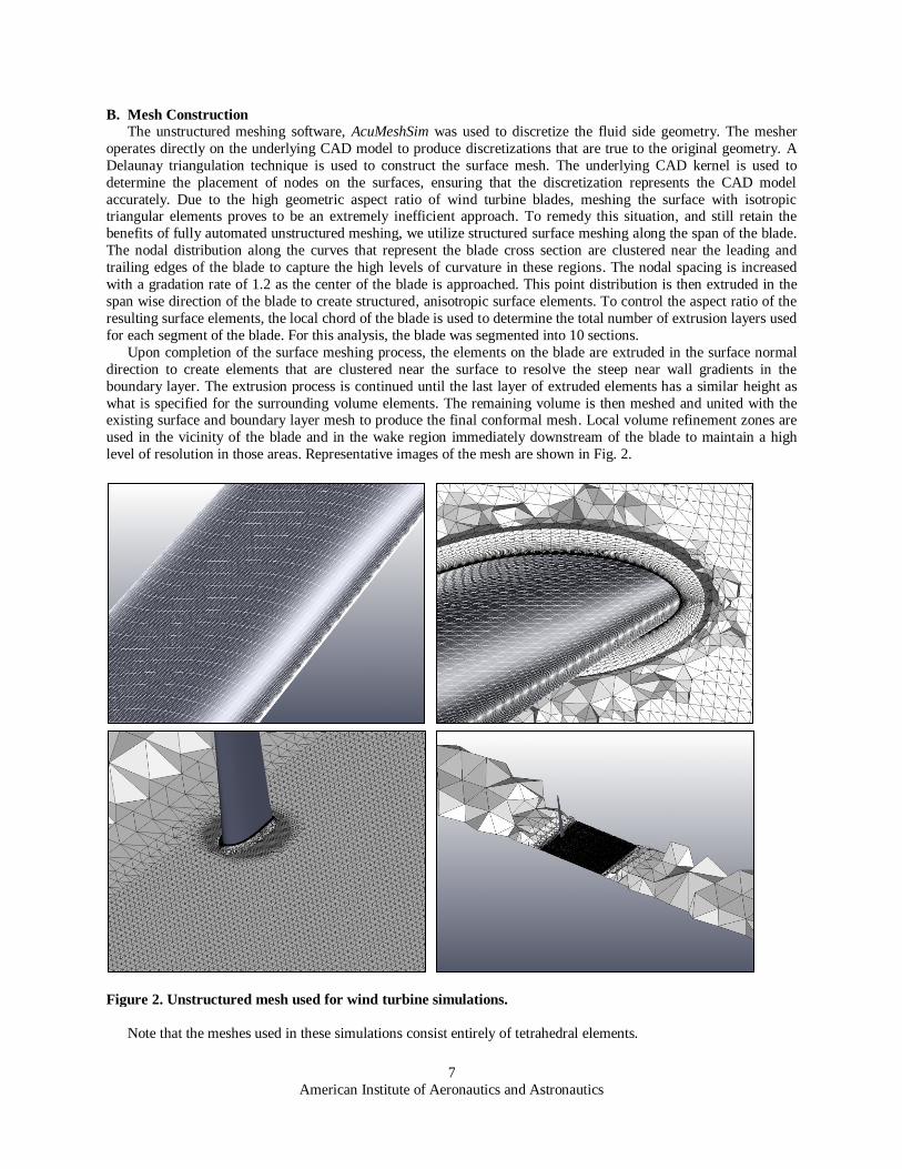
B. Mesh Construction
The unstructured meshing software, AcuMeshSim was used to discretize the fluid side geometry. The mesher
operates directly on the underlying CAD model to produce discretizations that are true to the original geometry. A
Delaunay triangulation technique is used to construct the surface mesh. The underlying CAD kernel is used to
determine the placement of nodes on the surfaces, ensuring that the discretization represents the CAD model
accurately. Due to the high geometric aspect ratio of wind turbine blades, meshing the surface with isotropic triangular elements proves to be an extremely inefficient approach. To remedy this situation, and still retain the
benefits of fully automated unstructured meshing, we utilize structured surface meshing along the span of the blade.
The nodal distribution along the curves that represent the blade cross section are clustered near the leading and
trailing edges of the blade to capture the high levels of curvature in these regions. The nodal spacing is increased
with a gradation rate of 1.2 as the center of the blade is approached. This point distribution is then extruded in the
span wise direction of the blade to create structured, anisotropic surface elements. To control the aspect ratio of the
resulting surface elements, the local chord of the blade is used to determine the total number of extrusion layers used
for each segment of the blade. For this analysis, the blade was segmented into 10 sections.
Upon completion of the surface meshing process, the elements on the blade are extruded in the surface normal
direction to create elements that are clustered near the surface to resolve the steep near wall gradients in the
boundary layer. The extrusion process is continued until the last layer of extruded elements has a similar height as
what is specified for the surrounding volume elements. The remaining volume is then meshed and united with the existing surface and boundary layer mesh to produce the final conformal mesh. Local volume refinement zones are
used in the vicinity of the blade and in the wake region immediately downstream of the blade to maintain a high
level of resolution in those areas. Representative images of the mesh are shown in Fig. 2.
Figure 2. Unstructured mesh used for wind turbine simulations.
Note that the meshes used in these simulations consist entirely of tetrahedral elements.

American Institute of Aeronautics and Astronautics
8
C. Modal Analysis
As mentioned previously, a modal representation of the blade structure is needed as input to the fluid model. For
this work, the structural dynamics of the blade were modeled using the RADIOSS finite element solver. A total of
100 eigenvalues were computed for this analysis. The eigenvalues that were computed represent the eigenvalues for
the undeformed and unloaded structure. All fluid loading and damping will be explicitly represented by the CFD
model. It should also be noted that the gravitational loading will not be included in the modal representation of the structure using the current approach. This is intentionally done due to the fluid simulation being done on a single
blade that maintains a fixed orientation.
The structure is modeled as a composite using a total of 207,360 shell elements. The nodes at the base of the
blade are constrained in all directions. The remainder of the model is left unconstrained.
D. Fluid Model Boundary Conditions
A uniform velocity profile was applied to the inlet boundary of the computational domain. This velocity was
chosen to match the appropriate wind speed for the rotor speeds of interest. A uniform eddy viscosity value was also
set at the inlet to model the turbulent diffusivity. The blade surfaces are modeled as a no-slip surface, with a wall
velocity matching the specified rotor speed at each radial location. For all simulations, a rotational frame of
reference was applied to the volume surrounding the rotor, with a velocity consistent with the rotor speed. When
multiple reference frames are used, AcuSolve transforms the velocity components into the appropriate frame to solve
the Navier-Stokes equations. The coriolis forces are added to the governing equations to simulate the rotation of the rotor wake as it propagates downstream. For all simulations, an integrated pressure outlet condition was applied to
the downstream boundary of the model domain. Slip conditions were applied to the remaining outer boundaries of
the cylindrical bounding volume. The cut faces of the 120 degree sector utilize rotationally periodic boundary
conditions. The nodes along the periodic axis are constrained to have no velocity in the cross-flow directions.
For simulations including flexible walls, the eigenvectors for each mode of the structure were projected onto the
wetted surface of the turbine blade. This projection procedure interpolates the eigenvectors between the dissimilar
meshes of the structure and fluid. For these applications, the velocity on the walls of the blades is the sum of the
velocity of each mode and that of the rotational speed of the rotor.
E. Mesh Motion Strategy
To keep the computational overhead to a minimum, a mesh motion strategy was devised that avoids the need to
solve the equations associated with the ALE approach. This was accomplished by projecting the nodes of the surrounding mesh onto the surface of the blade. The
motion of the surrounding nodes is then “driven” by
the element on the surface that it projected into. This
technique was seen to perform extremely well for this
application, resulting in a robust and computationally
efficient mesh motion strategy that allowed for a wide
range of structural motions. Fig. 3 depicts the motion
graphically by rendering iso-surfaces of wall distance
from the blade surface. The blue surface represents a
distance of 1 meter, while the gray surface represents
a distance of 30 meters. All nodes falling within the
volume of the blue surface were forced to move in unison with the blade. This approach preserves the
near wall structure of the boundary layer mesh. The
displacement of the nodes falling between the blue
iso-surface and the gray iso-surface is linearly scaled
from 1 at a distance of 1 m from the blade surface to a
value of zero at a distance of 30 m. This creates a
linearly tapered motion of the mesh surrounding the
blade. All other nodes in the domain are fixed to have
no motion. This approach does enforce a hard limit of approximately 30 meters of displacement of the blade in any
direction. However, this can easily be overcome by expanding the distance away from the blade at which the motion
is scaled to zero.
Figure 3. Illustration of the mesh motion scaling
distances used in moving mesh simulations.

American Institute of Aeronautics and Astronautics
9
F. Solver Settings
For steady state simulations, the flow equations were iterated to convergence using an infinite time step size
(1.0e10 seconds). Small amounts of incremental updating were used to increase the rate of convergence. Typical
simulations converged in approximately 50 non-linear iterations. Convergence was deemed sufficient when the
normalized change in pressure and velocity at each node in the simulation fell below 1.0e-2 and when the
normalized imbalance among forces at each node fell below 1.0e-3 for the flow equations and 1.0e-2 for the turbulence equation.
For transient simulations, two nonlinear iterations were performed at each time step to converge the equations to
a suitable level before moving on to the next time step. Past experience using AcuSolve for transient simulations of
wind turbines has resulted in a guideline that involves setting the time step size based on the tip speed of the blade.
The time step is typically fixed at a value that corresponds to advancing the rotor by 2 degrees of revolution per step.
Past experience with wind turbine simulations has shown this solution process to be sufficient to accurately resolve
the flow structures. However, it should be noted that full FSI simulations require additional care when selecting the
time step size and non-linear convergence criteria. The time stepping approach must be selected such that it can
resolve the time scales of the flow as well as those of the modes of vibration that are of interest. For these
simulations, the highest modal frequency that was included in the analysis is 27.45 Hz. To resolve this frequency,
the time step size for transient simulations was further reduced from the criteria described above to meet the Nyquist
criteria for resolving the 27.45 Hz signal. This resulted in a time step size of .018 sec.
IV. Simulation Results
A. Mesh Sensitivity Study A mesh sensitivity study was performed to ensure that the results of the simulations were mesh independent. Past
experience with the CFD simulation of wind turbines has revealed the aspects of the mesh design that the results are
most sensitive to. Perhaps the most critical parameter for obtaining accurate results of wind turbine blades is the
boundary layer resolution used in the simulations. In addition to that, the resolution of the leading and trailing edges
plays a significant role in ensuring accurate results from the CFD simulation. For all of the meshes described in this
paper, we utilize a near wall spacing of 5.0e-6 meters with a wall normal stretch ratio of 1.2. This results in an
average y+ value of ~1.0 for the rated power wind speed of the rotor. Although this requirement has been found to be excessively stringent for AcuSolve when using the Spalart-Allmaras turbulence model, the meshes were built to
enable the flexibility to investigate other turbulence models that have more demanding near wall meshing
requirements.
A total of 4 meshes were investigated. Each mesh utilized successively finer resolution of the blade surface and
volume surrounding the blade. Table 1 shows the parameters that were investigated, as well as the resulting mesh
size.
Mesh # Volume Mesh
Size (m)
Blade Surface
Mesh Size (m)
Surface
Anisotropy Level
Leading Edge
Mesh Size (m)
Trailing Edge
Mesh Size (m)
Number of
Nodes
1 .38 .38 6 .0152 .0608 2,276,706
2 .285 .285 4.5 .0114 .0456 4,994,212
3 .19 .19 3 .0076 .0304 7,593,941
4 .1425 .095 2 .0076 .0304 20,705,573
Table 1. Mesh controls used for mesh sensitivity study.
A single operating point of the wind turbine was selected, and a steady RANS simulation was performed using
each of the meshes listed above. The results of the simulation were compared based on the total power, total thrust, sectional loading of the blade, and pressure coefficient at various radial locations. Although the steady RANS
simulation does not necessarily reflect the complete physics of the aeroelastic simulations, it does provide a
significant reduction in compute cost for performing the mesh sensitivity study when compared to performing this
operation on a transient, aeroelastic simulation. The turbine is assumed to be operating with a constant wind profile
at rated power for this exercise. This corresponds to a wind speed of 11.3 m/sec and a rotation rate of 7.44 RPM.

American Institute of Aeronautics and Astronautics
10
Table 2 displays the total thrust and power computed for each of the meshes. The table reflects a very modest
sensitivity of both thrust and power to the mesh density. A full doubling of the mesh density resulted in less than 1%
change in thrust, and approximately 1.25% change in
power. Despite this small change in parameters, the
results warrant a closer look. Thrust and power are integrated quantities that may mask local variations in the
behavior of the flow around the blade. To better
investigate the local behavior of the flow between the
different meshes, the sectional loading and pressure
coefficient are analyzed.
For the purpose of interrogating the sectional loads on
the blade, it was subdivided into 2000 segments in the span wise direction. The pressure and viscous forces at each
segment were computed, decomposed into their cartesian components, and then integrated over the area of the
section. The resulting integrated loads are plotted in Fig. 4.
Figure 4. In plane and out of plane sectional loads.
Slight differences between the datasets are seen in the sectional in plane loading. The coarsest model, mesh 1,
shows a higher loading near the root of the blade than the other meshes. This over prediction in loading near the root
of the blade seems to be overshadowed by the under prediction in loading that is seen at the outer portions of the
blade, resulting in a total power prediction that is less than that of the refined meshes. Observation of the in plane
loading also indicates that meshes 3 and 4 show nearly identical results throughout the radial extent of the blade.
The out of plane loading shows good agreement between meshes 2,3, and 4. In comparison to the power, this
implies that the thrust is less sensitive to the mesh refinement.
The pressure coefficient provides another metric that is used to evaluate the simulation results. This quantity was
computed at various locations along the blade span and compared for each of the meshes that were investigated. Good agreement is seen between the simulation results at the out board stations. However, there is some mesh
sensitivity present at the in-board stations. This is reflected in Fig. 5.
A review of the mesh sensitivity study results reveals a consistent trend. Small changes are seen in the results
when increasing the mesh resolution up to that of mesh 3. As the mesh is further refined, no significant changes are
observed. With this in mind, mesh 3 is used for all subsequent simulations presented in this work. The settings used
for mesh 3 correspond to a leading edge initial spacing of 1/1000th of the maximum chord; a surface and volume
mesh size equal to 1/40th of the maximum chord, and a trailing edge initial spacing of 1/250th of the maximum
chord. Note that additional investigation of the meshing controls could be done to further optimize the mesh size,
but the current results are deemed sufficient for this work.
Mesh # Rotor Thrust (kN) Rotor Power (MW)
1 1883.2 13.94
2 1870.2 13.98
3 1872.7 14.12
4 1871.0 14.12
Table 2. Thrust and power results from mesh
sensitivity study.

American Institute of Aeronautics and Astronautics
11
Figure 5. Representative plots of pressure coefficient.
B. Comparison of AcuSolve, FAST, and WT_Perf Results
Once a suitable mesh density was determined, the CFD model was compared against simulation results from the
FAST and WT_Perf codes. At the current time, there is no test data available to compare the results of the
simulations against. However, the comparison of the CFD results against FAST and WT_Perf will act as a cross
comparison of the various simulation approaches and provide some level of confidence in the technique.
A power sweep of the 100m blade was performed using AcuSolve, FAST, and WT_Perf. For the AcuSolve
simulations, a steady state solution approach was employed, using the Spalart-Allmaras RANS model. Two different
types of simulations were performed. The first approach assumed a completely rigid structure. When performing this
type of simulation, AcuSolve converges directly to the time averaged flow field by iterating the solution to a steady state. The second set of simulations that was performed employed a steady state solution procedure that incorporated
flexible blades. Using this technique, AcuSolve is continuously updating the position of the blade in response to the
flow forces. The solution is iterated to convergence in the same manner as the rigid simulations were, and the
resulting deformation represents the mean deformed shape of the blade. These two simulation techniques allow
direct comparison of the rotor thrust, flapwise bending moment, power, and tip displacement against the FAST
results. WT_Perf does not contain a structural representation of the blade, and therefore, only the aerodynamic
quantities are compared against the other simulation techniques.
The Sandia 100 m blade design operates using a combination of speed control and pitch control. When operating
below rated power, the rotor speed is adjusted to control the power output. As the rotor reaches its rated power, the
blade pitch is changed to reduce the
loads resulting from increasing wind speed. This control strategy is
reflected in the operating points that
were used for the power sweep. This
data is shown in Table 3. The power
sweep begins at the cut-in speed of
3.0 m/s and concludes at 17.0 m/s.
Note that the cut-out speed of the
rotor is 25 m/s, but simulations were
not carried out at the higher wind
speeds.
The rotor thrust, rotor power, and flapwise bending moment were
tabulated and compared for the
AcuSolve, FAST, and WT_Perf
simulations. Fig. 6 shows that
excellent agreement is obtained for
the power predictions amongst all three codes up to the 11.3 m/s wind speed. As the wind speed increases beyond
this operating point, the blade pitch is changed to control the power output of the machine. Once the pitch control is
Wind Speed (m/s) Rotor Speed (RPM) Blade Pitch (degrees)
3.0 4.342 0.0
4.0 4.638 0.0
5.0 5.063 0.0
6.0 5.65 0.0
7.0 6.59 0.0
8.0 6.933 0.0
9.0 7.036 0.0
10.0 7.157 0.0
11.0 7.291 0.0
11.3 7.401 0.0
12.0 7.438 3.231
13.0 7.438 6.166
15.0 7.438 10.12
17.0 7.438 13.26
Table 3. Operating points used in power sweep.

American Institute of Aeronautics and Astronautics
12
active, the AcuSolve results show some discrepancies when compared to FAST and WT_Perf. The CFD approach is
predicting consistently lower values of power. As the wind speed and blade pitch are further increased above the
11.3 m/s operating point, the disagreement grows. The aerodynamics become increasingly complex in these
operating conditions and differences are expected
between the full solution of the RANS equations and
the techniques employed by FAST and WT_Perf. Closer inspection of the results showed that the FAST
simulations predict a constant power output of 14.0
MW above the 11.3 m/s wind speed, while WT_Perf
shows a peak power output of 14.1 MW at the 12 m/s
wind speed, and decreases slightly to 13.9 MW at the
17.0 m/s wind speed. The AcuSolve result shows a
peak power of 14.1 MW at a wind speed of 11.3 m/s,
then steadily decreases to 12.4 MW at the 17.0 m/s
wind speed.
Also of interest from this data is the difference in
predictions from AcuSolve when incorporating the
flexible structure. No significant, consistent trend is seen as a result of including the deformation of the
structure. Only a minor change in power and thrust is
observed when the blade is allowed to deform.
The good agreement for power prediction amongst
the three codes is encouraging. A further investigation of the aerodynamic predictions for the rotor is made by
investigating the rotor thrust and flapwise bending moment for the blade. The thrust provides a comparison of the
total forces acting on the blade in the streamwise direction, while the bending moment gives some indication of how
the forces are distributed radially along the blade. Figure 7 shows the comparison of these metrics for the three
simulation approaches. Despite the good agreement that was seen for power, we see significant differences between
the three codes when comparing the thrust. The AcuSolve results compare very well to WT_Perf, whereas the FAST
results show an over prediction in thrust at all wind speeds when compared against the others. Interestingly, the elevated level of thrust predicted by FAST appears to be nearly constant at 500 kN for all wind speeds.
Accompanying this increased level of thrust is an increase in the flapwise bending moment. We see again that the
WT_Perf and AcuSolve results agree very well when comparing the flapwise bending moment, while FAST tends to
show a higher value.
The excellent agreement between AcuSolve and WT_Perf tends towards the conclusion that FAST is providing
an over prediction of thrust and bending moment. Over prediction of these quantities by FAST was also
documented by Resor20 when comparing results against a technique that included a higher fidelity aerodynamic and
structural model.
Figure 6. AcuSolve, FAST, and WT_Perf predictions
for rotor power.
Figure 7. AcuSolve, FAST, and WT_Perf predictions for rotor thrust and flapwise bending moment.

American Institute of Aeronautics and Astronautics
13
Despite the disagreement in rotor thrust and bending moment between FAST and AcuSolve, the in plane and out
of plane blade tip displacement are compared between the two codes. Fig. 8 shows reasonable agreement between
the two approaches for in plane tip deflection up to a wind speed of 12 m/s. Beyond this point, the AcuSolve results
indicate a reduction in tip deflection whereas the FAST results show an increasing deflection up to the 15.0 m/s
wind speed. The out of plane tip deflection trends compare well between AcuSolve and FAST. Both models show
an increasing deflection up to the 11.3 m/s wind speed, with a reduction in deflection at wind speeds beyond that operating point. As expected, however, the FAST model shows consistently higher out of plane deflections, owing
to the increased thrust and bending moment that was observed previously.
Figure 8. AcuSolve and FAST predictions for blade tip deflection.
AcuSolve, FAST, and WT_Perf all show similar predictions for rotor power for this application. However, there
are significant differences between the simulation approaches for thrust, bending moment, and the resulting tip
displacement. AcuSolve and WT_Perf show excellent agreement for thrust and bending moment, whereas FAST
tends to over predict both of these quantities. The resulting tip displacements for FAST are also significantly higher
than what is predicted by AcuSolve. In the absence of test data to compare against, none of the aforementioned
approaches can be considered fully validated for this application. The agreement between the CFD results and the
WT_Perf model instills a high level of confidence that the AcuSolve model is accurately predicting the aerodynamic performance of the blade. The comparison of tip displacements between AcuSolve and FAST is not as favorable, but
this is attributed to the over prediction of thrust and bending moment that has been reported by other researchers.
Although the absolute agreement is poor for the out of plane tip displacements, the trends between the models are
similar, instilling confidence in the structural aspects of the AcuSolve model. With this in mind, the AcuSolve model
was extended to investigate the blade flutter phenomena.
C. Flutter Simulations
The primary goal of this work is to develop a fully coupled, high fidelity modeling approach that is capable of
predicting complex aeroelastic phenomena such as blade flutter. The desired end point is a validated modeling
approach that incorporates the full aerodynamic loading and structural response that is reflective of an operating
turbine. This includes fluctuating wind speeds due to turbulent structures that are ingested by the rotor as well as
effects associated with the wake of the machine. A logical starting point for the validation of the CFD based approach to flutter prediction is through a reproduction of existing results. Griffith and Ashwill1 present estimates of
the flutter speed for the 100 m blade using a technique developed by Lobitz18. The Lobitz approach focuses solely
on the influence of the shed wake for each individual blade and neglects the impact of the incident wind. This is
accomplished by modeling the blade as a fixed wing with spatially varying wind loads along its span. The technique
has provisions for adding centrifugal loading to the structure to better simulate the actual behavior of a wind turbine
blade. To predict the onset of flutter using this technique, the eigenvalues of the structural system at the selected
rotor speed are analyzed. Eigenvalues that have minimal or negative damping are assumed to be prone to flutter and
can be used to identify the flutter speed. Using this technique, the flutter speed of the rotor was approximated at 1.0-
1.1 times the maximum operating speed of the machine. The blade was held at a constant pitch of zero degrees
during the Sandia analysis, regardless of rotor speed.

American Institute of Aeronautics and Astronautics
14
Lobitz’s frequency based analysis is a deviation from the fully coupled, transient approach to aeroelasticity
developed here. However, the technique can be roughly reproduced using the current approach by modeling the
blade in still air. The rotational speed of the blade can be slowly ramped up until the flutter phenomenon is
observed. Initial investigations of the flutter speed will therefore focus on this type of numerical experiment to
provide a comparison against the already available predictions.
The wind turbine model used in previous sections of this work was extended to simulate the rotor in still air with a time varying rotor speed. To minimize the modifications to the model in comparison to the previously run cases,
an inlet velocity of 1.0e-4 m/s was specified to simulate the still air condition. This value is negligibly small and not
expected to impact the results. The rotor speed was started at 80% of the maximum speed then ramped using
discrete intervals to a speed of 2.0 times the maximum rotor speed. At each ramping interval, the rotor speed was
increased by 10% of the maximum rated speed over a time of ~1 second. The speed was then held constant for ~26
seconds before the rotor speed was increased once again. During this exercise, the tip speed and displacement was
monitored and used to evaluate the behavior of the blade.
Figure 9. Tip speed and displacement for ramped rotor speed flutter simulations.
Fig. 9 illustrates the behavior of the blade as the rotor speed is increased. The plot of tip speed shows the ramping profile used in the simulation. The plot of tip displacement indicates the motion of the blade as it responds
to the changing flow forces. The initial increase in speed at each ramp interval perturbs the system enough to initiate
a vibration in the blade. For the in plane direction, this motion appears to decay in time as the rotor speed is held
constant. The amplitude of the oscillation then grows rapidly the next time the system is perturbed by a variation in
rotor speed. The out of plane motion, however, exhibits significantly different behavior. This motion is characterized
by an initial displacement that corresponds to the aerodynamic thrust associated with the rotational speed of the
rotor. The blade is also vibrating about this position with a smaller amplitude oscillation. At the lower rotor speeds
(i.e. below max operating speed), the oscillation is fairly consistent about a mean displacement. However, an
interesting behavior is observed as the rotor is ramped to its maximum operating speed. The drastic increase in the
mean tip displacement indicates a significant change in the thrust. The tip continues to displace in the out of plane
direction for the duration that the rotor speed is held at the max rotor speed setting. Upon increasing the speed again,
the mean tip displacement decreases until reaching the 1.4x rotor speed condition where it begins a cyclic pattern of decreasing with increasing rotor speed. Superimposed on this large time scale displacement is a higher frequency,
low amplitude vibration. As was seen with the in plane displacements, this oscillation does not appear to be growing
in amplitude in any fashion that indicates the onset of blade flutter.
The results of the ramped rotor speed simulations are challenging to interpret. Additional simulations are
required to investigate the behavior of the blade in detail. Increasing the duration of time for which each operating
speed was held constant would help in understanding the response of the blade better. However, the overall behavior
of the blade does not indicate any onset of flutter in the simulation. One concern from the results is that the
displacements are fairly small in all cases. It is possible that the magnitude of the oscillations is insufficient to
trigger a large scale variation in the flow to further excite the structure. To test this hypothesis, a second set of
numerical experiments was performed. For these simulations, a fixed rotor speed was selected, and the blade was
perturbed by an impulse force. The force was ramped up from zero for 5 steps, held at its maximum amplitude for 5 steps, and then ramped back down to zero for 5 time steps. Once the force was removed, the blade was allowed to

American Institute of Aeronautics and Astronautics
15
oscillate freely. A total of 4 simulations were performed using this approach. Rotor speeds of 1.0, 1.1, 1.2, and 1.3
times the maximum rated rotor speed were investigated. In all cases, a still air condition was simulated using the
small inlet velocity of 1.0e-4 m/s.
Figure 10. Tip displacement for fixed rotor speed flutter simulations.
Fig. 10 shows that all rotor speeds investigated were characterized by an initial perturbation caused by the high
amplitude displacement in the in plane and out of plane directions. After the initial displacement has passed, a
smaller amplitude oscillation appears in both the in plane and out of plane directions. For the in plane direction, the
oscillation appears to sustain itself for the duration of the simulation, but with a very low amplitude. For the out of
plane motion, the behavior is characterized by a high frequency oscillation superimposed on top of a drifting
displacement towards a mean displaced state. For the time record that was simulated, the high frequency oscillation
in the in plane direction is seen to nearly disappear completely, while the large scale drift still appears. Longer time
record simulations are necessary to fully understand the behavior of the blade under these conditions. However, the
time record that was simulated indicates a decay of this signal, and no evidence of any type of fluid-elastic coupling that may lead to an undamped oscillation of the blade.
V. Summary and Conclusions
A Computational Fluid Dynamics based modeling approach has been developed to enable fully coupled FSI simulations of wind turbine rotors. The approach was first demonstrated on both a rigid and flexible blade using
steady state modeling techniques. Comparison of these results with WT_Perf simulations of the 100m blade
indicated favorable agreement. Comparisons to FAST showed deviations in thrust, bending moment, and tip
displacement. However, the deviations reflect an over prediction of these quantities by FAST that has been
documented by other researchers and is believed to be attributed to the aerodynamics model employed by the code.
Overall, the aerodynamic predictions of the CFD models were judged to be in excellent agreement with accepted
techniques, and the CFD models were extended to investigate the aeroelastic stability of the blade. To accomplish
this, the performance of the rotor was evaluated using numerical experiments geared towards reproducing the
configuration that is modeled using the Lobitz approach to aeroelastic stability. This involves simulation of the blade

American Institute of Aeronautics and Astronautics
16
in still air to identify the rotor speed at which it begins to develop a fluid elastic instability. Sandia’s initial analysis
of this blade using the Lobitz approach revealed very little margin to flutter. Their analysis resulted in a predicted
flutter speed between 1.0 and 1.1 times the maximum rated rotor speed. The flutter simulations performed on the
Sandia blade using the CFD based technique showed markedly different behavior. Two different attempts were
made at predicting the flutter speed of the blade using the CFD based approach. The first technique was
conceptually similar to what is prescribed by Lobitz; the rotational speed of the rotor was increased slowly to determine when the structural oscillations begin to grow in an undamped fashion. The rotor speed was ramped to a
value of 2 times the maximum rated rotor speed. The results of this exercise showed no proclivity of the blade to
flutter. One question regarding these results was the relatively small perturbations seen in the displacement of the
blade. A second set of CFD simulations was performed to address this. The second approach focused on the
simulation of a blade operating at a single, fixed rotor speed. The blade was displaced using an impulse force to
excite the structure. The blade was then allowed to oscillate freely. This exercise was performed for a total of 4 rotor
speeds, representing 1.0, 1.1, 1.2, and 1.3 times the maximum rated rotor speed. In all cases, the response of the
blade was seen to decay in time, and again, no indications of flutter were evident. It should be noted that the
simulations performed in this work represent a starting point for the development of the CFD model. The conditions
that were simulated were chosen to mimic the conditions that were previously utilized in Sandia’s aeroelastic model
of the 100m blade, while at the same time reducing some of the assumptions that are made in the analyses. This does
lead to some potentially significant variations in the simulation techniques. For example, the CFD approach used here incorporates the effect of the wake of the other blades of the machine by modeling the entire rotor through the
use of periodic boundary conditions. The impact of this is not known. Due to the early stage of this work and the
radically different approaches used by Sandia’s initial investigation of aeroelastic stability and the current one,
minimal effort was expended in investigating the differences between the results.
This work represents the first step towards the development of a validated CFD based modeling approach for
simulating the aeroelastic behavior of wind turbine blades. The work described here represents a deviation from
techniques developed in the past through the use of a high resolution fluid model to predict the aeroelastic
performance of the blade. Validation work will continue on the 100m blade model in pursuit of a high resolution
aeroelastic model that can simulate the behavior of the turbine under realistic operating conditions. This goal
requires extensions to the existing fluid and structural models. The fluid model will be enhanced to contain
realistic wind flow conditions including variable velocity wind profiles, gusts, and off axis loading cases. The structural model will be extended to include gravitational loading, centrifugal loading, and spin softening.
Acknowledgements
Sandia is a multiprogram laboratory operated by Sandia Corporation, a Lockheed Martin Company for the United
States Department of Energy’s National Nuclear Security Administration under contract DE-AC04-94AL85000.
References 1 Griffith, D.T. and Ashwill, T.D, "The Sandia 100-meter All-glass Baseline Wind Turbine Blade: SNL100-00," Sandia
National Laboratories Technical Report, June 2011, SAND2011-3779. 2 NWTC Design Codes (FAST by Jason Jonkman). http://wind.nrel.gov/designcodes/simulators/fast/. Last modified 12-August-2005; accessed 12-August-2005.
3 MSC.ADAMS Software, http://www.mscsoftware.com. Last accessed 10-August-2010. 4 NWTC Design Codes (AeroDyn by Dr. David J. Laino). http://wind.nrel.gov/designcodes/simulators/aerodyn/. Last
modified 05-July-2005; accessed 05-July-2005. 5 O.Sahni, M.Zhou, M.S. Shephard and K.E.Jansen, “Scalable Implicit Finite Element Solver for Massively Parallel
Processing with Demonstration to 160K cores”, Proceedings of the 2009 ACM/IEEE Conference on Supercomputing, 2009
ACM Gordon Bell Finalist, Portland, OR, USA, Nov. 2009. 6 Hughes, T.J.R., Franca, L.P. and Hulbert, G.M., 1989, "A new finite element formulation for computational fluid
dynamics.VIII. The Galerkin/least-squares method for advective-diffusive equations", Comp. Meth. Appl. Mech. Engg., 73, pp 173-189.
7 Shakib, F., Hughes, T.J.R. and Johan, Z., 1991, "A new finite element formulation for computational fluid dynamics. X. The compressible Euler and Navier-Stokes equations", Comp. Meth. Appl. Mech. Engg., 89, pp 141-219.
8 Jansen, K. E. , Whiting, C. H. and Hulbert, G. M., 2000, "A generalized-alpha method for integrating the filtered Navier- Stokes equations with a stabilized finite element method", Comp. Meth. Appl. Mech. Engg.", 190, pp 305-319.
9 Spalart, P.R. and Allmaras, S.R., 1992, “A one-equation Turbulence Model for Aerodynamic Flows”, 30th AIAA
Aerospace Sciences Annual Meeting, Reno NV, USA, 6-9 January, AIAA Paper No. 92-0439.
American Institute of Aeronautics and Astronautics
17
10 Spalart, P., Deck, S., Shur, M., Squires, K., Strelets, M. and Travin, A., 2006 "A New Version of Detached-Eddy Simulation, Resistant to Ambiguous Grid Densities", J. Theoretical and Computational Fluid Dynamics, 20, 181-195.
11 Godo, M.N, Corson, D. and Legensky, S.M., 2009, “An Aerodynamic Study of Bicycle Wheel Performance using CFD”, 47th AIAA Aerospace Sciences Annual Meeting, Orlando, FL, USA, 5-8 January, AIAA Paper No. 2009-0322. 12 AcuSolve, General Purpose CFD Software Package, Release 1.7f, ACUSIM Software, Mountain View, CA, 2009.
13 Lyons, D.C., Peltier, L.J., Zajaczkowski, F.J., and Paterson, E.G., 2009 “Assessment of DES Models for Separated Flow From a Hump in a Turbulent Boundary Layer”, J. Fluids Engg, 131, 111203-1 – 111203-9.
14 Bagwell, T.G., “CFD Simulation of Flow Tones From Grazing Flow Past a Deep Cavity”, Proceedings of 2006 ASME International Mechanical Engineering Congress and Exposition, Nov. 5-10, 2006, Chicago, Illinois.
15 Johnson, K and Bittorf, K., “Validating the Galerkin Least Square Finite Element Methods in Predicting Mixing Flows in Stirred Tank Reactors”, Proceedings of CFD 2002, The 10th Annual Conference of the CFD Society of Canada, 2002.
16 Godo, M.N, Corson, D. and Legensky, S.M., 2010, “A Comparative Aerodynamic Study of Commercial Bicycle Wheels using CFD”, 48th AIAA Aerospace Sciences Annual Meeting, Orlando, FL, USA, 4-7 January, AIAA Paper No. 2010-1431.
17 Spalart, P.R., Jou, W.-H, Strelets, M., Allmaras, S.R., “Comments on the feasibility of LES for wings, and on a hybrid RANS/LES approach”, Proceedings of the first AFOSR International Conference on DNS/LES, Ruston, Louisiana. Greyden Press, 4-8 Aug. 1997.
18 Lobitz, D.W., “Aeroelastic Stability Predictions for a MW-Sized Blade”, Wind Engineering, 2004, 7:211-224. 19 Resor, B.,Paquette, J., “Uncertainties in Prediction of Wind Turbine Blade Flutter”, 52nd AIAA/ASME/ASCE/AHS/ASC
Structures, Structural Dynamics and Materials Conference, 4-7 April, 2011, Denver, Colorado, AIAA Paper 2011-1947. 20 Resor, B.,Wilson, D., Berg, D., Berg, J., Barlas, T., Wingerden, J., Kuik, G. , “Impact of Higher Fidelity Models on
Simulation of Active Aerodynamic Load Control for Fatigue Damage Reduction”, 48th AIAA Aerospace Sciences Meeting and
Exhibit, 4-7 January, 2010, Orlando, Florida, AIAA Paper 2010-253. 21 NWTC Design Codes (WT_Perf by Marshall Buhl). http://wind.nrel.gov/designcodes/simulators/wtperf/. Last modified
17-February-2011; accessed 17-February-2011.


