
8/3/2019 Investigation of an Oscillating Surface Plasma for Turbulent Drag Reduction
http://slidepdf.com/reader/full/investigation-of-an-oscillating-surface-plasma-for-turbulent-drag-reduction 1/20
For permission to copy or to republish, contact the copyright owner named on the fir st page.
For A I A A -held copyright, write to A I A A Per missions Depar tment,
1801 A lexander B ell Dr ive, Suite 500, R eston, VA, 20191-4344.
41st Aerospace Sciences Meeting & Exhibit
6-9 January 2003
Reno, Nevada
AIAA 2003-1023
Investigation of an Oscillating Surface
Plasma for Turbulent Drag Reduction
Stephen P. Wilkinson
NASA Langley Research Center
Hampton, VA 23681-2199

8/3/2019 Investigation of an Oscillating Surface Plasma for Turbulent Drag Reduction
http://slidepdf.com/reader/full/investigation-of-an-oscillating-surface-plasma-for-turbulent-drag-reduction 2/20
AIAA 2003-1023
American Institute of Aeronautics and Astronautics
1
Invited Paper
INVESTIGATION OF AN OSCILLATING SURFACE PLASMA FOR
TURBULENT DRAG REDUCTION
Stephen P. Wilkinson*
NASA Langley Research Center, Hampton, VA
Abstract
An oscillating, weakly ionized surface plasma has been investigated for use in
turbulent boundary layer viscous drag
reduction. The study was based onreports showing that mechanical
spanwise oscillations of a wall canreduce viscous drag due to a turbulent
boundary layer by up to 40%. It washypothesized that the plasma induced
body force in high electric field
gradients of a surface plasma along stripelectrodes could also be configured to
oscillate the flow. Thin dielectric
panels with millimeter-scale, flush-mounted, triad electrode arrays with one
and two-phase high voltage excitationwere tested. Results showed that while a
small oscillation could be obtained, the
effect was lost at a low frequency (<100Hz). Furthermore, a mean flow was
generated during the oscillation that
complicates the effect. Hot-wire and
pitot probe diagnostics are presentedalong with phase-averaged images
revealing plasma structure.
Introduction
Dielectric-controlled, weakly ionized
AC surface plasmas operating at ______________________________ * Senior Research Engineer , Flow Physics andControl Branch, Senior Member AIAA
"This material is declared a work of the U.S.
Government and is not subject to copyright protection in the United States"
atmospheric pressure have recently
become a topic of interest for flowcontrol applications
1-6. The interest
stems from the plasma’s ability
to accelerate ionized air in regions of steep electric field gradients along strip
electrode edges. The combination of steep edge gradients and charged
particles within the plasma lead to a body force on the air through an
electrodynamic collisional process7. The
existence of the body force has led tothe search for flow control opportunities
that can utilize such an effect.
The plasma is typically generated
between adjacent, thin, surface, stripelectrodes with an intervening dielectric
to prevent avalanche breakdown of the
air. The most common configuration isthin foil strip electrodes bonded to
opposite sides of a thin dielectric panel.
The plasma is typically operated in the
range of 1-10kHz, 1-10kV rms for themajority of low speed experiments and
applications studied thus far. Some of
the physical principles on which the plasma and body force generation
operate are discussed by Roth1,2,5,7,8
and
Massines9. Kunhardt10 reviews this andsimilar plasmas and cites additional
references.
The present flow control investigationconsiders the possibility of reducing
viscous drag due to boundary layer
8/3/2019 Investigation of an Oscillating Surface Plasma for Turbulent Drag Reduction
http://slidepdf.com/reader/full/investigation-of-an-oscillating-surface-plasma-for-turbulent-drag-reduction 3/20
AIAA 2003-1023
American Institute of Aeronautics and Astronautics
2
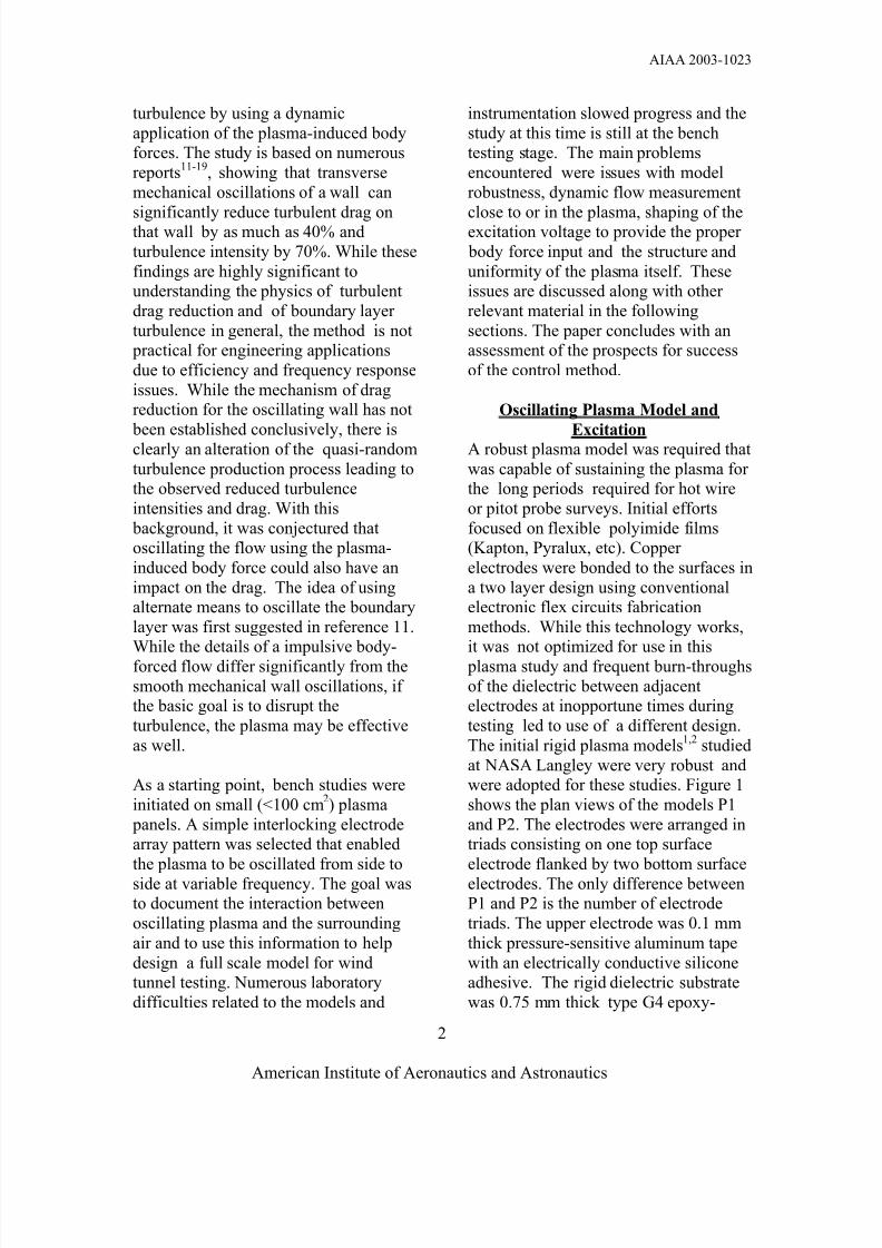
turbulence by using a dynamic
application of the plasma-induced bodyforces. The study is based on numerous
reports11-19
, showing that transverse
mechanical oscillations of a wall can
significantly reduce turbulent drag onthat wall by as much as 40% and
turbulence intensity by 70%. While these
findings are highly significant tounderstanding the physics of turbulent
drag reduction and of boundary layer
turbulence in general, the method is not practical for engineering applications
due to efficiency and frequency response
issues. While the mechanism of dragreduction for the oscillating wall has not
been established conclusively, there isclearly an alteration of the quasi-random
turbulence production process leading tothe observed reduced turbulence
intensities and drag. With this
background, it was conjectured thatoscillating the flow using the plasma-
induced body force could also have an
impact on the drag. The idea of usingalternate means to oscillate the boundary
layer was first suggested in reference 11.While the details of a impulsive body-
forced flow differ significantly from the
smooth mechanical wall oscillations, if the basic goal is to disrupt the
turbulence, the plasma may be effective
as well.
As a starting point, bench studies were
initiated on small (<100 cm2) plasma
panels. A simple interlocking electrodearray pattern was selected that enabled
the plasma to be oscillated from side to
side at variable frequency. The goal wasto document the interaction between
oscillating plasma and the surrounding
air and to use this information to help
design a full scale model for windtunnel testing. Numerous laboratory
difficulties related to the models and
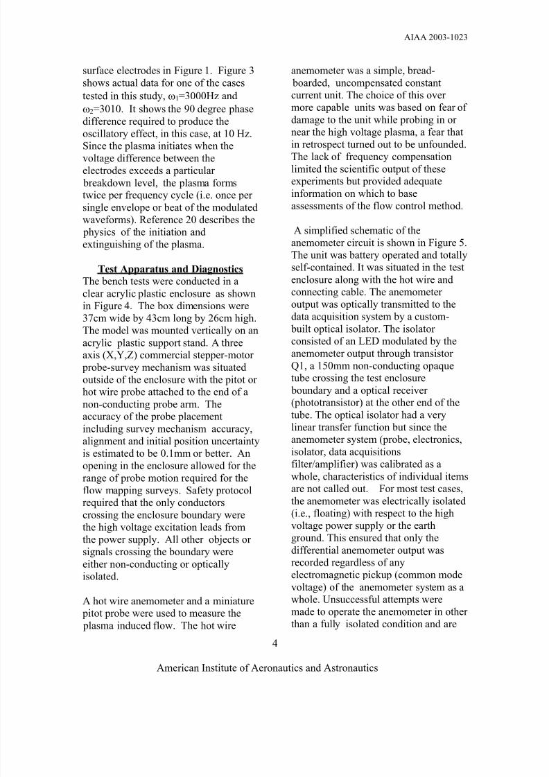
instrumentation slowed progress and the
study at this time is still at the benchtesting stage. The main problems
encountered were issues with model
robustness, dynamic flow measurement
close to or in the plasma, shaping of theexcitation voltage to provide the proper
body force input and the structure and
uniformity of the plasma itself. Theseissues are discussed along with other
relevant material in the following
sections. The paper concludes with anassessment of the prospects for success
of the control method.
Oscillating Plasma Model and
ExcitationA robust plasma model was required that
was capable of sustaining the plasma for the long periods required for hot wire
or pitot probe surveys. Initial efforts
focused on flexible polyimide films(Kapton, Pyralux, etc). Copper
electrodes were bonded to the surfaces in
a two layer design using conventionalelectronic flex circuits fabrication
methods. While this technology works,it was not optimized for use in this
plasma study and frequent burn-throughs
of the dielectric between adjacentelectrodes at inopportune times during
testing led to use of a different design.
The initial rigid plasma models1,2
studied
at NASA Langley were very robust andwere adopted for these studies. Figure 1
shows the plan views of the models P1
and P2. The electrodes were arranged intriads consisting on one top surface
electrode flanked by two bottom surface
electrodes. The only difference betweenP1 and P2 is the number of electrode
triads. The upper electrode was 0.1 mm
thick pressure-sensitive aluminum tape
with an electrically conductive siliconeadhesive. The rigid dielectric substrate
was 0.75 mm thick type G4 epoxy-

8/3/2019 Investigation of an Oscillating Surface Plasma for Turbulent Drag Reduction
http://slidepdf.com/reader/full/investigation-of-an-oscillating-surface-plasma-for-turbulent-drag-reduction 4/20
AIAA 2003-1023
American Institute of Aeronautics and Astronautics
3
woven glass printed circuit board. The
models were hand-built with theelectrodes registered from top to bottom
visually for a nominal zero electrode
overlap as shown. The aluminum tape
was bonded to the surface by dragging asmooth, blunt tool along the tape while
pressing down along the surface to
ensure a secure bond. A 1.2mm thick piece of float glass was bonded to the
bottom surface with a slow-cure, low
vapor pressure epoxy adhesive designedfor use in vacuum systems. The glass
provided a smooth mounting surface for
the model and suppressed the bottomsurface plasma. The bottom electrodes
were encapsulated in the epoxy betweenthe G4 dielectric and glass backing plate.
Small voids were visible through theglass in the epoxy between adjacent
electrodes but no model failures were
experienced with this constructiontechnique. Additional pieces of
aluminum tape (not shown) were affixed
to the numbered edge terminals for attachment of the high voltage excitation
clip leads.
The models were typically run at an
excitation frequency of 3 kHz. Higher frequencies led to more frequent
failures. At 6 kHz, models would fail
routinely after only short periods of
operations. At 10 kHz, only intermittentoperations (< 1 minute) could be
sustained due to model ignition. Non-
plastic dielectrics are more robust butnot without problems. One model used
thin float glass ( a biological specimen
slide) and failed by a microscopic burn-through, presumably at an imperfection
site in the glass after sustained use at
3kVrms and 3kHz.
A simplified schematic of the plasma
power supply is shown in Figure 2. The
input for each channel was provided by a
precision, synthesized sine wavegenerator. The high voltage amplifiers
(not shown) were commercial AC
variable frequency power supplies rated
at 1kVA each (one per channel). Thetransformers were custom-built 25:1
turns ratio with a center-tapped
secondary. They were rated at 1kVAeach. ( The power supplies were rated
for larger wind tunnel models, not for
the small bench test models shown inFigure 1). Each channel was capable of
providing in excess of 10kV rms, more
than adequate for the present study runat typically 3 kV rms.
The object was to create a oscillating
plasma on the upper surface. In Figure 2,the driving voltages are V1-V3 and V2-
V3. The trigonometric difference
relations for the two voltages assumingfor simplicity unity amplitudes are:
)sin()sin( 1231 t t V V ω ω −=−
[ ] [ ]t t )(sin)(cos2 1221
1221
ω ω ω ω −+= 1(a)
)sin()sin( 1232 ω ω +=−V V
[ ] [ ]t t )(cos)(sin2 1221
1221
ω ω ω ω −+= 1(b)
Note that voltages V1 and V2 are in anti-
phase and cause the voltage difference,
sin(ω2)-sin(ω1), in 1(a) to become a voltage
sum, sin(ω2)+sin(ω1), in 1(b). Equations
1(a) and 1(b) are the driving voltages for
the plasma. Each is seen to consist of ahigh frequency component (one half of
the sum of the input frequencies)
modulated by a low frequency
component ( one half of the difference of the input frequencies). The two signals
are in quadrature or 90 degrees out of
phase. This quadrature excitation provides the required input to drive the
plasma from side to side on the top
8/3/2019 Investigation of an Oscillating Surface Plasma for Turbulent Drag Reduction
http://slidepdf.com/reader/full/investigation-of-an-oscillating-surface-plasma-for-turbulent-drag-reduction 5/20
AIAA 2003-1023
American Institute of Aeronautics and Astronautics
4
surface electrodes in Figure 1. Figure 3
shows actual data for one of the cases
tested in this study, ω1=3000Hz and
ω2=3010. It shows the 90 degree phase
difference required to produce the
oscillatory effect, in this case, at 10 Hz.Since the plasma initiates when the
voltage difference between the
electrodes exceeds a particular
breakdown level, the plasma formstwice per frequency cycle (i.e. once per
single envelope or beat of the modulated
waveforms). Reference 20 describes the physics of the initiation and
extinguishing of the plasma.
Test Apparatus and DiagnosticsThe bench tests were conducted in a
clear acrylic plastic enclosure as shown
in Figure 4. The box dimensions were37cm wide by 43cm long by 26cm high.
The model was mounted vertically on an
acrylic plastic support stand. A threeaxis (X,Y,Z) commercial stepper-motor
probe-survey mechanism was situated
outside of the enclosure with the pitot or hot wire probe attached to the end of a
non-conducting probe arm. Theaccuracy of the probe placement
including survey mechanism accuracy,
alignment and initial position uncertaintyis estimated to be 0.1mm or better. An
opening in the enclosure allowed for the
range of probe motion required for the
flow mapping surveys. Safety protocolrequired that the only conductors
crossing the enclosure boundary were
the high voltage excitation leads from
the power supply. All other objects or signals crossing the boundary were
either non-conducting or opticallyisolated.
A hot wire anemometer and a miniature pitot probe were used to measure the
plasma induced flow. The hot wire
anemometer was a simple, bread-
boarded, uncompensated constantcurrent unit. The choice of this over
more capable units was based on fear of
damage to the unit while probing in or
near the high voltage plasma, a fear thatin retrospect turned out to be unfounded.
The lack of frequency compensation
limited the scientific output of theseexperiments but provided adequate
information on which to base
assessments of the flow control method.
A simplified schematic of the
anemometer circuit is shown in Figure 5.The unit was battery operated and totally
self-contained. It was situated in the testenclosure along with the hot wire and
connecting cable. The anemometer output was optically transmitted to the
data acquisition system by a custom-
built optical isolator. The isolator consisted of an LED modulated by the
anemometer output through transistor
Q1, a 150mm non-conducting opaquetube crossing the test enclosure
boundary and a optical receiver (phototransistor) at the other end of the
tube. The optical isolator had a very
linear transfer function but since theanemometer system (probe, electronics,
isolator, data acquisitions
filter/amplifier) was calibrated as a
whole, characteristics of individual itemsare not called out. For most test cases,
the anemometer was electrically isolated
(i.e., floating) with respect to the highvoltage power supply or the earth
ground. This ensured that only the
differential anemometer output wasrecorded regardless of any
electromagnetic pickup (common mode
voltage) of the anemometer system as a
whole. Unsuccessful attempts weremade to operate the anemometer in other
than a fully isolated condition and are

8/3/2019 Investigation of an Oscillating Surface Plasma for Turbulent Drag Reduction
http://slidepdf.com/reader/full/investigation-of-an-oscillating-surface-plasma-for-turbulent-drag-reduction 6/20
AIAA 2003-1023
American Institute of Aeronautics and Astronautics
5
discussed in the Results - Hot-Wire and
Pitot Probe Issuessection.
The hot wire probe consisted of a single
5 micron platinum-plated tungsten wire,
approximately 1.5mm long. Theanemometer circuit was designed to run
the probe at a fixed nominal resistance
or overheat ratio of 1.5. The probe wascalibrated in a small, compressed air
open jet adjacent to the test enclosure
using the same probe cable as for the plasma measurements. The maximum
calibration velocity was about 2.5 m/sec.
The no-flow output voltage was offset tonominally zero and low pass filtered
appropriate to the test (typically 10 Hzfor DC measurements and 0.1-3 kHz for
dynamic data). Calibration data was fitto a fourth order polynomial for
converting raw data to velocity.
The anemometer was not temperature
compensated which caused a drift bias
error as the probe was moved from thecalibration jet to the test enclosure and
during the plasma runs. No preciseattempt was made to quantify error
although observing the no-flow zero
shifts suggests that a 15-20% absoluteerror is likely. For a given run, however,
under constant conditions and using the
same calibration, the relative magnitudes
should be much better. The quantitativeanemometer data should, therefore, be
used judiciously. Other important hot
wire issues such as behavior in or near plasma, frequency compensation, wire
orientation, wall proximity effects and
use in a still air environment arediscussed with presentation of the actual
data.
A pitot probe was also used in one set of mean flow measurements. It consisted of
a 1 mm OD by 0.1mm wall thickness
stainless steel tube. The probe end was
flattened to 1.35 mm wide by 0.57mmhigh. Dynamic pitot pressure was
referenced to the atmosphere and
measured with a 10mmHg full scale
capacitive gage. The pressure accuracyis 0.01%, however, the derived velocity
accuracy depends on flow angularity,
wall effects and possible plasma effectsmaking the absolute accuracy difficult to
predict. As in the case of the hot wire
data, any quantitative data for the pitottube should be used judiciously.
The plasma was photographed to obtaininstantaneous and phase averaged photos
of its structure. An intensified charge-coupled-device (ICCD) camera (Cooke
Corp. DiCam Pro SVGA) was used witha long distance microscope lens. The
camera’s image intensifier used a S20
photocathode and a P43 phosphor screen. The ICCD camera was triggered
by a delay timer circuit. The circuit
received an input pulse from one of the plasma signal generator's sync output
and delivered a variable width, variabledelay trigger pulse to the camera. The
trigger pulse width determined the
duration of the exposure. Since thevoltage and current in the plasma are
approximately 90 degrees out of phase
(due to the transformer-coupled power
supply), the phase-average was based onthe current waveform. Figure 6 shows a
typical trigger with respect to the plasma
current. In this case, a 10 microsecondICCD capture occurs at the
instantaneous anode and cathode of the
plasma. The basic camera output was1280x1024 pixels which was binned
with a 2x2 factor to increase brightness.
The combination of short exposure, a
dim plasma and the microscopic lensrequired that binning (accumulation of
neighboring pixels into one) be used to

8/3/2019 Investigation of an Oscillating Surface Plasma for Turbulent Drag Reduction
http://slidepdf.com/reader/full/investigation-of-an-oscillating-surface-plasma-for-turbulent-drag-reduction 7/20
AIAA 2003-1023
American Institute of Aeronautics and Astronautics
6
obtain a visible image against the
background noise even with the imageintensifier. The ICCD camera
acquisition rate (frame rate) to the
computer memory was about 20 frames
per second.
The plasma excitation voltage and
currents were measured with a 20kV,75kHz 1000:1 high voltage probe and a
100 kHz bandwidth current monitoring
toroidal transformer. Voltages V1, V2 and V3 in Figure 2 were measured with
the high voltage probes and driving
voltage differences V1-V3 and V2-V3 were formed with two analog op-amp
difference circuits. All dynamic datawas acquired with a 1Ghz band-width
digital oscilloscope. The particular model used had enhanced resolution and
peak detection modes that proved very
useful in these experiments. Theenhanced resolution uses real time
averaging to increase voltage resolution
and reduce noise. The peak detectionmode combines data from several time
sweeps to capture short duration voltagespikes that may otherwise not be
recorded. This was particularly useful in
capturing plasma current waveforms.
RESULTS
ICCD images
Figure 6 shows phase-averaged images
on the plasma along an electrode edge
under steady state excitation. Thecamera’s image acquisition input trigger
is shown with respect to the plasma
current waveform above each photograph. The shape of the current
waveform and the location of the plasma
breakdown varies with model size and
design (electrical load). The currentwaveform was acquired in enhanced
resolution mode on the oscilloscope
which suppresses the high amplitude
noise due to the plasma breakdown. Thecamera is focussed on a plan view of
the electrode and the top surface
electrode edge is horizontal along the
bottom portion of each image. Thedigital images have been enhanced to
improve display quality. Each image was
processed with an un-sharp mask toimprove contrast and a median filter to
reduce noise. The trigger pulse was 10
microseconds in duration. The CCDsensor in the camera only acquired data
while the trigger level was high. These
photo’s were obtained for one of theflex-circuit Kapton models used early in
the study. The electrode is copper in thiscase. The aluminum tape models
showed the same behavior.
The image on the left was taken when
the top electrode was the instantaneousanode corresponding the positive
current half-cycle and the photo on the
right for the negative half-cycle or cathode. Looking ahead at Figure
13(b), the total duration of the plasmafor either the anode or cathode is about
150-160 µsec out of the total cycle
period of 333 µsec. For the remaining
cycle time, no plasma light is observed.This shows that there are clearly two
distinct plasma “pulses” per excitation
cycle, one for the instantaneous anode
and one for the instantaneous cathode.
There are two primary and significant
features evident in the Figure 6 images.
First, the plasma distribution along theelectrode edge is very non-uniform. This
is presumably due to local irregularitiesor asperities along the electrode’s edge.
An attempt was made to polish the
electrode edge on a different, hand-builtaluminum-tape-electrode model. While
the uniformity can be increased

8/3/2019 Investigation of an Oscillating Surface Plasma for Turbulent Drag Reduction
http://slidepdf.com/reader/full/investigation-of-an-oscillating-surface-plasma-for-turbulent-drag-reduction 8/20
AIAA 2003-1023
American Institute of Aeronautics and Astronautics
7
somewhat, there appear to be limited
gains with this approach. The secondnoteworthy feature is the fundamentally
different structure of the anode and
cathode images. Whereas the anode
image resemble discrete “fountains” , thecathode image shows clear structure in
closed loops and bridging across peaks
of the plasma structures. In both images,the location of the structures was very
repeatable. On an instantaneous basis,
within any single 10 microsecond trigger duration, only 1 or 2 flashes of light
occur which accumulate with averaging
into the images shown. It is clear,therefore, that the plasma is both
spatially and temporally non-uniform.The extent to which this non-uniformity
affects the induced body force, flowuniformity and device efficiency is not
known. Additional ICCD phase
averaged images are presented with the pitot probe data regarding plasma
formation on the pitot probe itself.
Hot-Wire and Pitot Probe Issues
Two dimensional hot-wire surveys were
conducted for models P1 and P2 with
both steady-state and oscillating plasmas. Before presenting this data
however, a number of issues with both
the hot-wire and pitot tube must first be
discussed. First, the plasma tests wereconducted in a still air environment
within the test enclosure. The absence of
an imposed free stream velocity causesinterpretation difficulties with both
instruments aside from any additional
considerations due to the plasma. Theelectrodes on both models are oriented
vertically and the surveys were
conducted in the X-Y plane. The single
element hot wire was therefore alsooriented vertically. Since there was no
free stream flow, the hot wire responds
mainly to the magnitude of the local 2D
velocity vector, (U2+V
2)**0.5, and not
the flow direction. The pitot tube on the
other hand will be in error to the extent
that the flow is not aligned with the tube
axis. As seen in the PIV measurementdata for a configuration similar to the
current models3, the angle can be as high
as 45 degrees away from the topelectrode. If the pitot probe is aligned
with the surface, the velocity error can
be significant.
The absence of a free stream flow makes
the hot wire subject to free convectioneffects at low velocities. The vertical
orientation of the hot wire causes athermal convection plume to develop
enveloping the wire. This plume adds tothe usual heat conduction wall
interference effect for data obtained very
close to the wall. As the probeapproaches the wall in still air, the plume
around the wire becomes restricted and
distorted decreasing cooling of the wire.This leads to an increase in wire
temperature and resistance which showsup as a velocity error. Figure 7 shows
that the error increases rapidly below
about Y=0.3mm. This is a worst casesince in practice, some velocity exists
near the wall which reduces the error.
The conclusion is that care must be
exercised in interpreting data very closeto the wall to see if it can be explained
by a wall proximity effect.
Another issue with the hot wire is the
use of an uncompensated anemometer.
There was no technical reason not tocompensate the wire. As mentioned
earlier, the issue was one of uncertainty
over possible electrical damage to the
circuit in the high voltage environment.Using a simple and inexpensive
anemometer to start with, confidence

8/3/2019 Investigation of an Oscillating Surface Plasma for Turbulent Drag Reduction
http://slidepdf.com/reader/full/investigation-of-an-oscillating-surface-plasma-for-turbulent-drag-reduction 9/20
AIAA 2003-1023
American Institute of Aeronautics and Astronautics
8
was built that with normal care, the
anemometer was not in any danger of damage due to any high voltage
phenomena. In fact, the anemometer
proved to be trouble free after weeks of
daily operation which included oneepisode in which the probe was
inadvertently grounded while
approaching a high voltage electrode.The hot wire prongs were instantly
destroyed but the directly connected
electronic anemometer circuit survivedunharmed. The frequency response issue
due to the lack of compensation is
discussed further with regard to theoscillating plasma results.
In order to obtain either hot wire or pitot
data in close proximity to the plasma, the problem of a glow discharge forming on
the probe itself was an issue. Since the
glow is associated with generation of a body force and acceleration of the air,
evidence of glow on the probe indicates
probable error in the data. In the case of the pitot probe, the actual dynamic
pressure at the probe tip can be reduced by a plasma-induced flow emanating
from the probe itself. This was
discovered while testing methods tomove the pitot probe closer to the top
electrode while avoiding a discharge due
to high polarization of the metallic
probe.
Figure 8 shows phase averaged ICCD
images (previously introduced for Figure6) of the pitot probe close to the upper
electrode. Four conditions are shown
each with anode and cathode triggering(see discussion of Figure 6). In
condition (a), the top electrode is at the
excitation voltage, the bottom electrode
(on the other side of the model, seeFigure 1) is grounded (V=0) and the
pitot probe is electrically isolated. No
glow on the probe is observed. If the
probe is moved closer to the electrode, afilamentary discharge (distinctly
different from the glow discharge
plasma) forms between the probe and the
electrode. To eliminate this discharge,the probe was tied to the excitation
voltage in (b). While the filamentary
discharge is eliminated (since theelectrode and probe are now at the same
potential) a glow discharge plasma
forms between the probe and the bottomelectrode through the dielectric panel.
Notice the distinctive anode and cathode
structure for each triggering condition.For this condition (b), the measured pitot
pressure was approximately zero. Thereason is that the pitot probe and top
electrode generate flow in oppositedirections.
For conditions (c) and (d), the voltage onthe top and bottom electrodes were
reversed. The condition where the top
electrode was at the excitation voltageand the probe grounded or visa-versa
was not possible since there would be nointervening dielectric to prevent arcing.
The image for condition (d), cathode
trigger, is missing but would be similar to (c ), cathode trigger, directly above it.
The images are reversed from (a) and (b)
since the trigger was derived from the
signal generator for the top electrode.
Steady-State Plasma – Mean Flow
Given the issues raised above withrespect to hot wire and pitot
measurements and the accuracy issue of
the hot wire due to temperature drift andalso the low speeds, Figure 9 shows a
comparison of the two techniques for a
steady, plasma-induced mean flow for
Model P1. Note that the that the sizes of the survey regions are different for the
hot wire and pitot data. The pitot region

8/3/2019 Investigation of an Oscillating Surface Plasma for Turbulent Drag Reduction
http://slidepdf.com/reader/full/investigation-of-an-oscillating-surface-plasma-for-turbulent-drag-reduction 10/20
AIAA 2003-1023
American Institute of Aeronautics and Astronautics
9
is a subset of the hot wire region. The
aspect ratio of the contour maps is 1:1.
The plots have some evident differences
in the color mappings but largely show
the same general structure. The hot wiremeasures velocity magnitude from any
direction and has a known wall
interference effect below about Y=0.5mm (see Figure 7). The pitot measures
stagnation pressure at the tip and will be
in error for any flow angularity. The pitot probe tip height is two orders of
magnitude greater than the hot wire
diameter and averages the pressure over the face of the probe. Given these
issues, the peak velocities of 1.6 and 1.3m/s for the hot wire and pitot
respectively appears to be reasonableresults. The maps suggest that the
maximum velocity lies to the left of the
map in the vicinity of the top electrodeas would be expected since that is the
location of the maximum electric field
gradient and body force. Since thisregion is within the plasma, discharges
from metallic probes limits probemeasurements in this area.
Figure 10 shows velocity magnitude profiles at seven X locations from the
hot-wire map of Figure 9. The curves
are spline curve fits to the actual data
and pass smoothly through each data point. The data symbols are not shown
for clarity. The figure shows
decelerating, broadening profilesconsistent with a wall jet as expected.
Some of the data is below Y=0.5mm and
at the lowest velocities, the wall proximity effect shown in Figure 7 is
applicable. Overall however, the data
seem to capture the structure of the flow
well.
Oscillating Plasma – Mean and
Fluctuating Flow
Models P1 and P2 were run with
oscillating plasmas over the range of 5-
80 Hz. The upper frequency
corresponded to the frequency at whichthe signal-to-noise ratio for the
anemometer approached unity. Hot wire
velocity magnitude data were acquiredon two dimensional grids similar to
Figure 9. The peak of the excitation
amplitudes (V1-V3 and V2-V3, seeFigures 2 and 3) were set to be the same
as for the steady state case. Figure 11
shows the relative rms amplitude of the peak fluctuating velocity near the top
electrode on model P1. The peak wasobtained from contour maps of the rms
amplitude at each test frequency.Tracking the peak rms was chosen over
monitoring a fixed spatial location since
the rms spatial distribution changed withfrequency. From 5 to 80 Hz, the peak
rms velocity moved 2.5mm closer to the
top electrode in the negative X direction. The data in Figure 11 are normalized by
the measured peak fluctuation rmsamplitude at 10Hz.
Also shown in Figure 11 is theuncompensated thermal response of a 5
micron Platinum-plated Tungsten wire
with microwave heating21
, the same size
and type of wire used in the currentexperiments. The frequency response of
the wire varies with stream velocity and
the data shown are for the case of zerostream velocity. The figure shows that
roll-off in the measured fluctuations
exceeds the roll-off in theuncompensated wire response. From 10
to 80 Hz, the model amplitude data
(symbols) fall by 15db with less than a
third of that attributable to theuncompensated hot-wire. Also, the data
roll-off at a rate consistent with that of a

8/3/2019 Investigation of an Oscillating Surface Plasma for Turbulent Drag Reduction
http://slidepdf.com/reader/full/investigation-of-an-oscillating-surface-plasma-for-turbulent-drag-reduction 11/20
AIAA 2003-1023
American Institute of Aeronautics and Astronautics
10
first order system or –20dB/decade as
shown by the dashed line. The reason for this response is not known. Discussion
of the frequency requirements for
oscillating the flow will be discussed in
the next section along with the impact of this finding.
Figures 12(a-d) are peak normalizedcontour plots of the mean and fluctuating
velocity magnitudes for model P2 at an
oscillation frequency of ω2-ω1=20 Hz.The vertical coordinate (Y) is stretched
by a factor of three to show more detailnear the wall. The thickness of the
dielectric panel is correct but the height
of the electrodes is exaggerated for visibility.
The unexpected feature of Figures 12(a)
and (c) is that a mean flow forms in thevicinity of the top electrodes. The
reason for this can be found in Figures
13(a) and 13(b). Figure 13(a) shows oneof the excitation signals from the power
supply (also shown in Figure 3) along
with the AC current through the model.
The noisy bulges in the currentwaveform correspond to plasmaformation along the electrodes. Figure
13(b) zooms in on a one millisecond
segment near the peak of one of the
voltage envelopes in Figure 13(a).(“Envelope” refers to the section of
increasing/decreasing voltage between
zero crossings in Figure 13(a)). As seenin Figure 13(b), the plasma forms twice
per excitation cycle, once for the anode
and once for the cathode with thecathode plasma being the more energetic
of the two. Figure 13(a) shows that
plasma duty cycle is about 65% of eachenvelope or equivalently, the plasma is
on 65% of the time on each electrode
edge. Recall that there are two excitation
signals 90 degrees out of phase (see
Figure 3). Since the duty cycle is greater
than 50%, the plasmas on each edge of the top electrode overlap in time, in this
case by 30%.
The plasma is clearly on for too long andcreates the undesirable mean flow. In
Figure 13(a), the plasma turns on shortly
after each voltage zero crossing betweenthe envelopes and turns off shortly
before each zero crossing. These points
correspond to the air breakdown voltage.For a sinusoidal excitation voltage and a
fixed breakdown threshold, the duty
cycle will vary with the amplitude of theexcitation voltage. In the limiting case
where the excitation amplitude is equalto the breakdown threshold, the duty
cycle is zero. As the excitationamplitude increases, so does the duty
cycle. The strength of the plasma and
body force depends upon the excitationamplitude. For an amplitude just above
the breakdown threshold, the duty cycle
will be short but the plasma will beweak. For an excitation amplitude much
greater than the breakdown threshold,the plasma will be strong but the duty
cycle will be long. Its clear that a
sinusoidal envelop is not well suited tothis application. A more suitably shaped
envelope allowing better control of the
strength of the plasma and the duty cycle
would be preferable.
Discussion
The results reported above provideinformation on the magnitude or relative
magnitude of plasma-induced velocities,
their penetration into the surrounding air and frequency response of the air to the
unsteady electrodynamic forcing. The
purpose of this discussion is to assess
this information with regard to therequirements for turbulent boundary

8/3/2019 Investigation of an Oscillating Surface Plasma for Turbulent Drag Reduction
http://slidepdf.com/reader/full/investigation-of-an-oscillating-surface-plasma-for-turbulent-drag-reduction 12/20
AIAA 2003-1023
American Institute of Aeronautics and Astronautics
11
layer drag reduction using an oscillating
wall as discussed in the introduction .
The references on oscillating wall drag
reduction11-19
indicate that drag
reduction occurs when the non-dimensional frequency is around 0.01
and the peak non-dimensional wall
displacement is greater than thespanwise low speed streak correlation
length. For estimating the plasma
induced motion requirements for a lowspeed wind tunnel test at 10 m/s, it is
assumed that F+=Fν/uτ
2=0.01 and
∆X+=∆X uτ/ν=100 are representative
values where a measurable effect would
be expected Assuming a sinusoidaloscillation and standard ambient
conditions of 760mmHg and 20 deg Cand an average skin friction coefficient of Cf
=0.004, these data correspond to a
plasma-induced motion requirement of F= 130.7 Hz and UX= 2.8 m/s where UX is the peak spanwise velocity.
If the absolute peak velocity in Figure 11
corresponding to 0 dB is assumed to be
1.6 m/s (from Figure 9), the data arealready below the target velocity of 2.8
m/s by about a factor of two. Whilethis could probably be corrected by
optimizing the electrode design and
increasing the excitation amplitude, thedata further roll-off at a high rate. At the
137 Hz target frequency, there was no
measurable oscillation signal above the
noise level. It is clear, therefore, that thetarget conditions for the proposed low-
speed drag-reduction test are not likely
to be attained with the current method.
Aside from the oscillatory aspects of the
problem, there are other physicalconsiderations. As opposed to the
oscillating wall, which is a smooth
translation over a wide area, the strip
electrodes are inherently three-
dimensional. It was shown in the first plasma flow control test at Langley
1,2,
that streamwise oriented plasma
electrodes generate unstable vortices
with steady state excitation due to the bi-lateral mean flow. In addition, even if
the plasma duty cycle problem discussed
earlier were corrected, as the oscillationfrequency increases, a behavior similar
to the steady-state results would be
expected. A further issue is that of scaling to flight conditions. If physics
and the non-dimensional frequency
requirement of F+=0.01 holds at flight
conditions, an unlikely situation, the
required frequency would be in excess of 1 MHz. Even if the scaling did not hold,
a frequency very much higher than thecurrent target of 137 Hz for a 10 m/s low
speed test would be expected. Overall,
the lack of adequate amplitude andfrequency response along with the three
dimensionality of the plasma electrodes
and mean flow effects indicate that the proposed approach will probably not
work as an alternative to themechanically oscillated wall.
There is no indication of any significantscalability in the method that would
allow use at the high Reynolds numbers
and high subsonic Mach numbers
required for flight. While the body forcestrength can be increased by increasing
the amplitude of the excitation voltage,
the breakdown strength of the dielectric becomes the limiting parameter. The
materials used in these experiments were
already selected based on their high breakdown voltage and further gains in
this area using currently available
materials would most likely be
incremental. Higher excitationfrequencies required in flight also
exacerbate the material robustness issue.

8/3/2019 Investigation of an Oscillating Surface Plasma for Turbulent Drag Reduction
http://slidepdf.com/reader/full/investigation-of-an-oscillating-surface-plasma-for-turbulent-drag-reduction 13/20
AIAA 2003-1023
American Institute of Aeronautics and Astronautics
12
In developing the models for the current
experiments doubling the excitationfrequency to 6 kHz caused a large
increase in the model failure (burn-
through) rate. Operation at 10 kHz
could only be done on an intermittent basis without igniting the plastic model.
The excursion into the phase-averagedICCD photographs was actually a
precursor to planned use of the camera
for particle flow visualization. Thatactivity has not yet been started but the
camera proved to be very useful in
capturing the structure of the plasma asseen in Figures 6 and 8. Since the
plasma body force is associated with thesteep electric field gradient at the
instantaneous cathode of a normal glowdischarge, only the cathode picture in
Figure 8 may be responsible for the gas
motion. While there are two plasma pulses per excitation cycle (Figure
13(b)), only one seems to be responsible
for the observed flow behavior. Thatraises the question as to what the anode
pulse does to the flow or to the systemefficiency.
Another issue raised by the Figure 6 and8 photographs has to do with theoretical
and computational modeling. Clearly,
one would prefer not to have to deal with
the spatial and temporal randomness andcomplexity of the observed plasma
patterns in order to compute the plasma
body force. The simplified force modelused in reference 3 indicates that this is
possible for steady state applications. A
simplified dynamic force model is alsorequired.
Summary and Conclusions
This study was an attempt to develop a plasma-based analog to a mechanically
oscillated wall. The guiding
consideration was that the lateral
oscillations were the operative feature incontrolling turbulence production, and
that the oscillations could be achieved in
various ways, such as, with a plasma-
induced flow. The current concept wasnot carried through to wind tunnel drag
measurements because bench testing
showed problems with the approach. Themain finding was that the plasma-
induced oscillations rolled off rapidly
with frequency and were not able tomeet the requirements for a low speed
test. Also, the oscillations were
accompanied by a bi-lateral mean flowalong the electrodes. Such motion is
characteristic of steady-state excitationand has been shown to cause streamwise
vortex formation. The prognoses,therefore, for this particular plasma drag
reduction approach is not favorable.
The study, however, produced
noteworthy findings with respect to the
plasma itself and experimental
techniques. Phase-averaged, 10 µsecduration photographs show distinctly
different, very non-uniform light patterns for the instantaneous anode andcathode. This could have implications
for flow modeling studies.
A successful model design andexcitation method were developed with
the triad electrode actuators driven by a
quadrature output power supply. Withrespect to diagnostics, the hot-wire
anemometer was shown to be a useful
tool for studying the plasma-inducedflow provided the entire unit is
electrically isolated. Even with isolation,
however, polarization discharge or glowdischarge from the probes can cause
significant measurement errors.

8/3/2019 Investigation of an Oscillating Surface Plasma for Turbulent Drag Reduction
http://slidepdf.com/reader/full/investigation-of-an-oscillating-surface-plasma-for-turbulent-drag-reduction 14/20
AIAA 2003-1023
American Institute of Aeronautics and Astronautics
13
In conclusion, the lack of success for
current study should not reflectunfavorably on the study of flow control
with plasma-induced motions in general.
A number of studies are currently
underway and no doubt more are planned. What the current study shows
is that applications should be sought on
scale in keeping with the plasma-induced body force strength limitations.
Instead of trying to oscillate the entire
wall region of the boundary layer, for example, a more focused approach
targeting local turbulent motions close to
the wall could be studied.
References
1. Roth, J.R., Sherman, D.M. and
Wilkinson, S.P., Boundary layer flow
control with a one atmosphere uniformglow discharge surface plasma, AIAA
paper 98-0328, 1998.
2. Roth, J.R., Sherman, D.M., and
Wilkinson, S.P., Electrohydrodynamicflow control with a glow-discharge
surface plasma. AIAA Journal. 38(7),
July 2000, pp. 1166-1172.
3. Corke, T.C., Jumper, E.J.
Post, M.L., McLaughlin, T.E.,
Application of weakly-ionized plasma as
wing flow control devices, AIAA paper 2002-0350, 2002
4. Lorber, P., McCormick, T.,Anderson, T., et al., Rotorcraft
Retreating Blade Stall Control, AIAA
paper A00-33875, 2000.
5. Roth, J.R., Method and apparatus for
covering bodies with a uniform glow
discharge plasma and applications
thereof. US Patent 5,669,583, Sept. 23,
1997.
6. Sherman, D.M., S.P. Wilkinson, and
J.R. Roth, Paraelectric Gas Flow
Accelerator. US Patent US 6200539 B1,March 13, 2001
7. Roth, J.R., Industrial PlasmaEngineering, Volume 2, Applications to
Nonthermal Plasma Processing. Vol. 2.,
Institute of Physics Publishing, 2001
8. Roth, J.R., Industrial Plasma
Engineering, Volume 1, Principles. Vol.1, Institute of Physics Publishing 1995,
pp. 453-461.
9. Massines, F., Rabehi, A.
Decomps, P., Gadri, R.B., et al.,Experimental and theoretical study of a
glow discharge at atmospheric pressurecontrolled by a dielectric barrier, Journal
of Applied Physics. 83(6), March 15,
1998, pp. 2950-2957.
10. Kunhardt, E.E., Generation of large-
volume, atmospheric-pressure
nonequilibrium plasmas. IEEETransactions on Instrumentation and
Measurements. 28(1), February, 2000
pp.189-200.
11. Akhavan, R., W. Jung, and N.Mangiavacchi, Control of wall
turbulence by high frequency spanwise
oscillations, AIAA Paper 93-3282, 1993.
12. Choi, J.-I., C.-X. Xu, and J.H. Sung,
Drag reduction by spanwise walloscillations in wall-bounded turbulent
flows, AIAA Journal, 40(5), May, 2002
pp.842-850.
13. Trujillo, S.M., D.G. Bogard, and
K.S. Ball, Turbulent boundary layer drag

8/3/2019 Investigation of an Oscillating Surface Plasma for Turbulent Drag Reduction
http://slidepdf.com/reader/full/investigation-of-an-oscillating-surface-plasma-for-turbulent-drag-reduction 15/20

8/3/2019 Investigation of an Oscillating Surface Plasma for Turbulent Drag Reduction
http://slidepdf.com/reader/full/investigation-of-an-oscillating-surface-plasma-for-turbulent-drag-reduction 16/20
AIAA 2003-1023
American Institute of Aeronautics and Astronautics
15
Figure 1. Plasma test models.
Dashed rectangle represents test
area. Numbers are terminal
designations. Black traces topsurface, gray traces bottom
surface. Units millimeters.
90
65 65
Model P1 Model P2
2
1
3
12
3
A sin(ω1t)
2Asin(ω2t)
V1
V2
V3
Figure 2. Plasma power supply
and model hook-up. Bars
represent top and bottom surface
electrodes. (Dielectric not shown.)
Figure 3. Example of differential
excitation voltage across
dielectric. In Figure 2, these
represent V1-V3 and V2-V3
Figure 4. Experimental bench
setup. (1) ICCD camera, (2) lens,
(3) clear plastic box enclosure, (4)
3-axis probe survey mechanism,
(5) non-conducting probe
extension arm, (6) hot-wire probe,
(7) anemometer, (8) opticalisolator, (9) cable to data
acquistion system, (10) plasma
model, (11) model support, (12)
plasma power leads
1
3
2
54
6
10
12
7
8
9
11
Time, sec
E x c i t a t i o n A m p l i t u d e ,
k V
5
0
-5
0
-5
0 0.1 0.2
Figure 1. Plasma test models.
Dashed rectangle represents test
area. Numbers are terminal
designations. Black traces topsurface, gray traces bottom
surface. Units millimeters.
90
65 65
Model P1 Model P2
2
1
3
12
3
90
65 65
Model P1 Model P2
2
1
3
12
3
A sin(ω1t)
2Asin(ω2t)
V1
V2
V3
A sin(ω1t)
2Asin(ω2t)
V1
V2
V3
Figure 2. Plasma power supply
and model hook-up. Bars
represent top and bottom surface
electrodes. (Dielectric not shown.)
Figure 3. Example of differential
excitation voltage across
dielectric. In Figure 2, these
represent V1-V3 and V2-V3
Figure 4. Experimental bench
setup. (1) ICCD camera, (2) lens,
(3) clear plastic box enclosure, (4)
3-axis probe survey mechanism,
(5) non-conducting probe
extension arm, (6) hot-wire probe,
(7) anemometer, (8) opticalisolator, (9) cable to data
acquistion system, (10) plasma
model, (11) model support, (12)
plasma power leads
1
3
2
54
6
10
12
7
8
9
11
Time, sec
E x c i t a t i o n A m p l i t u d e ,
k V
5
0
-5
0
-5
0 0.1 0.2
Time, sec
E x c i t a t i o n A m p l i t u d e ,
k V
5
0
-5
0
-5
0 0.1 0.2

8/3/2019 Investigation of an Oscillating Surface Plasma for Turbulent Drag Reduction
http://slidepdf.com/reader/full/investigation-of-an-oscillating-surface-plasma-for-turbulent-drag-reduction 17/20
AIAA 2003-1023
American Institute of Aeronautics and Astronautics
16
Figure 5. Schematic of
hot-wire anemometer and
optical isolator.
0 0.2 10.80.60.4
0
0.4
0.2
0.1
0.3
Y, mm
Figure 7. Hot wire wall proximity
effect in still air. Overheat ratio
R hot/R cold=1.5, R cold ~ 3.5Ω , 5µm
diameter platinum-plated Tungsten.Wall and wire axis vertical. Prongs
normal to wall.
10
-10
0I, mA
T , uS0 300-300
10
-10
0I, mA
T , uS0 300-300
Figure 6. ICCD phase-averaged photographs of plasma along edge of electrode.
Plots show camera trigger with respect to plasma current. Camera exposure: 10µsec per shot, 20 shots per photograph. Excitation: ~8.5kVp-p at 3kHz.
Anode
Cathode
9 mm 9 mm
R 1 R 2
R 3R w R 4
R 5 Q1
LED
Phototransistor
+V -V
R 6
C1
A1 A2
+-
-
+
+V
+V
Output
+V
+V+VFigure 5. Schematic of
hot-wire anemometer and
optical isolator.
0 0.2 10.80.60.4
0
0.4
0.2
0.1
0.3
Y, mm
Figure 7. Hot wire wall proximity
effect in still air. Overheat ratio
R hot/R cold=1.5, R cold ~ 3.5Ω , 5µm
diameter platinum-plated Tungsten.Wall and wire axis vertical. Prongs
normal to wall.
10
-10
0I, mA
T , uS0 300-300
10
-10
0I, mA
T , uS0 300-300
Figure 6. ICCD phase-averaged photographs of plasma along edge of electrode.
Plots show camera trigger with respect to plasma current. Camera exposure: 10µsec per shot, 20 shots per photograph. Excitation: ~8.5kVp-p at 3kHz.
10
-10
0I, mA
T , uS0 300-300
10
-10
0I, mA
T , uS0 300-300
Figure 6. ICCD phase-averaged photographs of plasma along edge of electrode.
Plots show camera trigger with respect to plasma current. Camera exposure: 10µsec per shot, 20 shots per photograph. Excitation: ~8.5kVp-p at 3kHz.
Anode
Cathode
9 mm9 mm 9 mm9 mm
R 1 R 2
R 3R w R 4
R 5 Q1
LED
Phototransistor
+V -V
R 6
C1
A1 A2
+-
-
+
+V
+V
Output
+V
+V+V
R 1 R 2
R 3R w R 4
R 5 Q1
LED
Phototransistor
+V -V
R 6
C1
A1 A2
+-
-
+
+V
+V
Output
+V
+V+V

8/3/2019 Investigation of an Oscillating Surface Plasma for Turbulent Drag Reduction
http://slidepdf.com/reader/full/investigation-of-an-oscillating-surface-plasma-for-turbulent-drag-reduction 18/20
AIAA 2003-1023
American Institute of Aeronautics and Astronautics
17
Top: V=Asin(ωt)
Bottom: V=0
Probe: isolated
Top: V=Asin(ωt)
Bottom: V=0
Probe: V=Asin(ωt)
Top: V=0
Bottom: V=Asin(ωt)
Probe: isolated
Top: V=0
Bottom: V=Asin(ωt)
Probe: V=0
Anode Trigger Cathode Trigger
Not Available
(a)
(b)
(c)
(d)
Figure 8. ICCD camera phase-averaged photographs
of pitot probe tip at various
electrical potentials. Excitation
voltage ~8.5kVp-p, 3kHz.
Exposure:10 µsec pr shot, 20
shots per photograph.
Top: V=Asin(ωt)
Bottom: V=0
Probe: isolated
Top: V=Asin(ωt)
Bottom: V=0
Probe: V=Asin(ωt)
Top: V=0
Bottom: V=Asin(ωt)
Probe: isolated
Top: V=0
Bottom: V=Asin(ωt)
Probe: V=0
Anode Trigger Cathode Trigger
Not Available
(a)
(b)
(c)
(d)
Figure 8. ICCD camera phase-averaged photographs
of pitot probe tip at various
electrical potentials. Excitation
voltage ~8.5kVp-p, 3kHz.
Exposure:10 µsec pr shot, 20
shots per photograph.
Figure 9. Contour maps (color) of mean velocity magnitudes from hot-wire and
pitot probes. Bracketed numbers are (X,Y) coordinates of corners of contour
maps in millimeters. Y=0, top surface; X=0, right edge of top electrode. Scale
and color legend different for each map. Excitation is single-phase 8.47kV p-p
at 3 kHz. Model is P1.
Hot-wire
Pitot
0 1.6 m/s
0 1.3 m/s
(28,6.3)
(4,0.1)
(14,1.5)
(3,0.1)

8/3/2019 Investigation of an Oscillating Surface Plasma for Turbulent Drag Reduction
http://slidepdf.com/reader/full/investigation-of-an-oscillating-surface-plasma-for-turbulent-drag-reduction 19/20
AIAA 2003-1023
American Institute of Aeronautics and Astronautics
18
Figure 11. System frequency response
measured with hot wire (symbols)
Log(F), Hz
5
0
-5
-10
-15
-200 1 2 3
uncompensated wire
Kidron (1966)
-20 dB/decade d B = 2 0 l o g ( U / U r e f )
Figure 10. Velocity magnitude profiles at
various X locations (denoted by labels in
mm)
Figure 12(a) and 12(b). Contour plots (color) of mean and fluctuating velocitymagnitude for Model P1 F=20 Hz. Excitation is two-phase 8.76 kV p-p at ω1=3000 and
ω2=3020 kHz. Map corner coordinates (X,Y) shown in parentheses. Color legends apply
to individual maps only. X=0 is right edge of top electrode; Y=0 is top surface.
0 1
0 1
(3,0.2)
(3,0.2)
(4.7,22.5)
(4.7,22.5)
Mean
Fluctuating RMS
Y, mm
V e l o c i t y M a g n i t u d e , m / s
0 2 4 60
1
4
7
10
13
16
24
19
Y, mm
V e l o c i t y M a g n i t u d e , m / s
0 2 4 60
1
4
7
10
13
16
24
19

8/3/2019 Investigation of an Oscillating Surface Plasma for Turbulent Drag Reduction
http://slidepdf.com/reader/full/investigation-of-an-oscillating-surface-plasma-for-turbulent-drag-reduction 20/20
AIAA 2003-1023
A i I i f A i d A i
19
Figure 13(a). Typical voltage and current
excitation waveforms (V1-V3 or V2-V3)
(peak normalized).
Figure 13(b). Expanded one millisecond time
interval of an envelope peak in 13(a).
Figure 12(c) and 12(d). Contour plots (color) of mean and fluctuating rms velocity
magnitude for Model P2. Excitation is 8.76 kV p-p atω1=3000 and ω2=3020 kHz. Map
corner coordinates (X,Y) are shown in parentheses. Color legends apply to individual
maps only. X=0 is mid point between upper electrodes; Y=0 is top surface.
0 1
0 1
(c) Mean
(d) Fluctuating RMS
(-10,1.7)
(10,4.2)
(10,4.2)
(-10,1.7)
0 50 100 150
1
0
-1
0
-1
Time, sec
V
I
0 50 100 150
1
0
-1
0
-1
Time, sec
V
I
1
0
-1
0
-1
-2
0 0.2 0.4 0.6 0.8 1.0
Time, msec
V
I
1
0
-1
0
-1
-2
0 0.2 0.4 0.6 0.8 1.0
Time, msec
V
I
msec


