
INV ITEDP A P E R
Hierarchical Modeling,Optimization, and Synthesisfor System-Level Analog andRF DesignsSmall models, that represent the overall functioning of portions of large
or complex circuits, can be generated by algorithms and used
for system design and verification.
By Rob A. Rutenbar, Fellow IEEE, Georges G. E. Gielen, Fellow IEEE, and
Jaijeet Roychowdhury, Senior Member IEEE
ABSTRACT | The paper describes the recent state of the art in
hierarchical analog synthesis, with a strong emphasis on
associated techniques for computer-aided model generation
and optimization. Over the past decade, analog design automa-
tion has progressed to the point where there are industrially
useful and commercially available tools at the cell levelVtools
for analog components with 10–100 devices. Automated tech-
niques for device sizing, for layout, and for basic statistical
centering have been successfully deployed. However, successful
component-level tools do not scale trivially to system-level
applications. While a typical analog circuit may require only 100
devices, a typical system such as a phase-locked loop, data
converter, or RF front-end might assemble a few hundred such
circuits, and comprise 10 000 devices or more. And unlike
purely digital systems, mixed-signal designs typically need to
optimize dozens of competing continuous-valued performance
specifications, which depend on the circuit designer’s abilities to
successfully exploit a range of nonlinear behaviors across levels
of abstraction from devices to circuits to systems. For purposes
of synthesis or verification, these designs are not tractable when
considered Bflat.[ These designs must be approached with
hierarchical tools that deal with the system’s intrinsic design
hierarchy. This paper surveys recent advances in analog design
tools that specifically deal with the hierarchical nature of
practical analog and RF systems. We begin with a detailed
survey of algorithmic techniques for automatically extracting a
suitable nonlinear macromodel from a device-level circuit. Such
techniques are critical to both verification and synthesis
activities for complex systems. We then survey recent ideas in
hierarchical synthesis for analog systems and focus in particular
on numerical techniques for handling the large number of
degrees of freedom in these designs and for exploring the space
of performance tradeoffs early in the design process. Finally, we
briefly touch on recent ideas for accommodating models of
statistical manufacturing variations in these tools and flows.
KEYWORDS | Computer-aided design; integrated circuits;
modeling; simulation
I . INTRODUCTION
Automated analog integrated circuit design is becoming a
viable solution for increasing design productivity for
critical analog components. Over the past decade, analog
design automation has progressed to the point wherethere are industrially useful and commercially available
tools at the cell levelVtools for analog components with
10–100 devices. Automated techniques for device sizing,
for layout, and for basic statistical centering have been
successfully deployed. Gielen and Rutenbar [2] offer a
fairly complete survey of the area. However, successful
component-level tools do not scale trivially to system-level
Manuscript received May 3, 2006.
R. A. Rutenbar is with the Department of Electrical and Computer Engineering,
Carnegie Mellon University, Pittsburgh, PA 15213-3890 USA
(e-mail: [email protected]).
G. G. E. Gielen is with ESAT-MICAS, Katholieke Universiteit Leuven, 3001 Leuven,
Belgium (e-mail: [email protected]).
J. Roychowdhury is with the Electrical and Computer Engineering Department,
University of Minnesota, Minneapolis, MN 55455 USA (e-mail: [email protected]).
Digital Object Identifier: 10.1109/JPROC.2006.889371
640 Proceedings of the IEEE | Vol. 95, No. 3, March 2007 0018-9219/$25.00 �2007 IEEE

applications. While a typical analog circuit may requireonly 100 devices, a typical system such as a phase-locked
loop, a data converter, or an entire RF front-end might
assemble a few hundred such circuits and comprise
10 000 devices or more. And unlike purely digital
systems, mixed-signal designs typically need to optimize
dozens of competing continuous-valued performance
specifications, which depend on the circuit designer’s
abilities to successfully exploit a range of nonlinear be-haviors across levels of abstraction from devices to circuits
to systems. Such designs are also increasingly being
integrated in large system-on-chip (SOC) environments,
in challenging (i.e., highly scaled digital CMOS [1])
fabrication processes. Verifying, optimizing, and synthe-
sizing such complex systems is generally not tractable
when they are considered Bflat.[ These designs must be
approached with hierarchical tools that deal with thesystem’s intrinsic design hierarchy. In any hierarchical
approach macromodels or behavioral models are the
bridge between the different levels in the hierarchy, both
top-down and/or bottom-up.
This paper surveys recent advances in analog design
tools that specifically deal with the hierarchical nature of
practical analog and RF systems. We begin in Section II
with a detailed survey of algorithmic techniques forautomatically extracting a suitable nonlinear macromodel
from a device-level circuit. Such techniques are critical to
both verification and synthesis activities for complex
systems; they allow us to simulate large systems, in practical
amounts of time, with just enough fidelity for the behaviors
we seek to model. We then survey in Section III recent
ideas in hierarchical synthesis and optimization for analog
systems. We focus in particular on numerical techniques forhandling the large number of degrees of freedom in these
designs and for exploring the space of performance tradeoffs
early in the design process. Finally, in Section IV we briefly
touch on recent ideas for accommodating models of
statistical manufacturing variations in these tools and flows.
Section V offers concluding remarks.
II . ALGORITHMIC MACROMODELINGTECHNIQUES
Electronic systems today, especially those for communica-
tions and sensing, are typically composed of a complex mix
of digital, analog, and RF circuit blocks. Simulating or
verifying such systems is critical for discovering and
correcting problems prior to fabrication, in order to avoid
refabrication which is typically very expensive. Simulatingentire systems to the extent needed to generate confidence
in the correctness of the to-be-fabricated product is,
however, also usually very challenging in terms of com-
putation time. Full transistor-level verification of large
systems can simply be prohibitive in terms of CPU time.
A common and useful approach towards verification in
such situations, both during early system design and after
detailed block design and layout, is to replace large and/orcomplex blocks by small macromodels that replicate their
input–output functionality well and to verify the macro-
modeled system. The macromodeled system can be
simulated rapidly in order to evaluate different choices
of design-space parameters. Such a macromodel-based
verification process affords circuit, system, and architec-
ture designers considerable flexibility and convenience
through the design process, especially if performedhierarchically using macromodels of differing sizes and
fidelity.
The key issue in the above methodology is, of course,
the creation of macromodels that represent the blocks of
the system well. This is a challenging task for the wide
variety of communication and other circuit blocks in use
today. The most prevalent approach towards creating
macromodels is manual abstraction. Macromodels areusually created by the same person who designs the
original block, often aided by simulations. While this is the
only feasible approach today for many complex blocks, it
does have a number of disadvantages compared to the
automated alternatives that are described in this paper.
Simulation often does not provide abstracted parameters
of interest directly (such as poles, residues, modulation
factors, etc.); obtaining them by manual postprocessing ofsimulation results is inconvenient, computationally ex-
pensive, and error prone. Manual structural abstraction of
a block can easily miss the very nonidealities or
interactions that detailed verification is meant to discover.
With semiconductor device dimensions shrinking below
100 nm and nonidealities (such as substrate/interconnect
coupling, degraded device characteristics, etc.) becoming
increasingly critical, the fidelity of manually generatedmacromodels to the real subsystems to be fabricated
eventually is becoming increasingly suspect. Adequate
incorporation of nonidealities into behavioral models, if at
all possible by hand, is typically complex and laborious.
Generally speaking, manual macromodeling is heuristic,
time consuming, and highly reliant on detailed internal
knowledge of the block under consideration, which is
often unavailable when subsystems that are not designedin-house are utilized. As a result, the potential time-to-
market improvement via macromodel-based verification
can be substantially negated by the time and resources
needed to first generate the macromodels.
It is in this context that there has been considerable
interest in automated techniques for the creation of
macromodels. Such techniques take a detailed description
of a blockVfor example, a SPICE-level circuit netlistVandgenerate, via an automated computational procedure, a
much smaller macromodel. The macromodel, fundamen-
tally a small system of equations, is usually translated into
Matlab/Simulink form for use at the system level. Such an
automated approach, i.e., one that remains sustainable as
devices shrink from deep submicron to nanoscale, is es-
sential for realistic exploration of the design space in
Rutenbar et al. : Hierarchical Modeling, Optimization, and Synthesis for System-Level Analog and RF Designs
Vol. 95, No. 3, March 2007 | Proceedings of the IEEE 641

current and future communication circuits and othersystem applications.
Several broad methodologies for automated macro-
modeling have been proposed. One is to generalize,
abstract, and automate the manual macromodeling
process. For example, common topological elements in a
circuit are recognized, approximated, and conglomerated
(e.g., [18] and [19]) to create a macromodel. Another class
of approaches attempts to generate symbolic macromodelsthat capture the system’s input–output relationship, e.g.,
[20]–[25]. Yet another class (e.g., [26]–[28]) employs a
black-box methodology. Data is collected via many
simulations or measurements of the full system and a
regression-based model is created that can predict outputs
from inputs. Various methods are available for the
regression, including data mining, multidimensional
tables, neural networks, genetic algorithms, etc.In this paper, we focus on another methodology for
macromodeling, often termed algorithmic. Algorithmic
macromodeling methods approach the problem as the
transformation of a large set of mathematical equations to a
much smaller one. The principal advantage of these
methods is generalityVas long as the equations of the
original system are available numerically (e.g., from within
SPICE), knowledge of the circuit structure, operatingprinciples, etc., is not critical. A single algorithmic method
may therefore apply to entire classes of physical systems,
encompassing circuits and functionalities that may be very
disparate. Four such classes, namely linear time-invariant(LTI), linear time-varying (LTV), nonlinear (nonoscillatory),
and oscillatory are discussed in this section. Algorithmic
methods also tend to be more rigorous about important
issues such as fidelity and stability, and often provide bet-ter guarantees of such characteristics than other methods.
A. Macromodeling LTI SystemsOften referred to as reduced-order modeling (ROM) or
model-order reduction (MOR), automated model generation
methods for LTI systems are the most mature among
algorithmic macromodeling methods. Any block composed
of resistors, capacitors, inductors, linear controlled sources,and distributed interconnect models is LTI (often referred
to simply as Blinear[). The development of LTI MOR
methods has been driven largely by the need to Bcompress[the huge interconnect networks, such as clock distribution
nets, that arise in large digital circuits and systems.
Replacing these networks by small macromodels makes it
feasible to complete accurate timing simulations of digital
systems at reasonable computational expense. Althoughinterconnect-centric applications have been the main
domain for LTI reduction, it is appropriate for any system
that is linear and time invariant. For example, Blinear
amplifiers,[ i.e., linearizations of mixed-signal amplifier
blocks, are good candidates for LTI MOR methods.
Fig. 1 depicts the basic structure of an LTI block. uðtÞrepresents the inputs to the system, and yðtÞ the outputs in
the time domain; in the Laplace (or frequency) domain
their transforms are UðsÞ and YðsÞ, respectively. The
definitive property of any LTI system [29] is that the inputand output are related by convolution with an impulse
response hðtÞ in the time domain, i.e., yðtÞ ¼ xðtÞ � hðtÞ.Equivalently, their transforms are related by multiplication
with a system transfer function HðsÞ, i.e., YðsÞ ¼ HðsÞXðsÞ.Note that there may be many internal nodes or variables
within the block. The goal of LTI MOR methods is to
replace the block by one with far fewer internal variables,
yet with an acceptably similar impulse response or transferfunction.
In the majority of circuit applications, the LTI block is
described to the MOR method as a set of differential
equations, i.e.,
E _x ¼ AxðtÞ þ BuðtÞyðtÞ ¼ CTxðtÞ þ DuðtÞ: (1)
In (1), uðtÞ represents the input waveforms to the block
and yðtÞ the outputs. Both are relatively few in numbercompared to the size of xðtÞ, the state of the internal
variables of the block. A, B, C, D, and E are constant
matrices. Such differential equations can be easily formed
from SPICE netlists or AHDL descriptions, especially for
interconnect applications, the dimension n of xðtÞ can be
very large.
The first issue in LTI ROM is to determine what aspect
of the transfer function of the original system should beretained by the reduced system; in other words, what
metric of fidelity is appropriate. In their seminal 1990
paper [30], Pileggi and Rohrer used moments of the
transfer function as fidelity metrics, to be preserved by the
model reduction process. The moments mi of an LTI
transfer function HðsÞ are related to its derivatives, i.e.,
m1 ¼dHðsÞ
ds
����s¼s0
; m2 ¼ d2HðsÞds2
����s¼s0
; � � � ; (2)
where s0 is a frequency point of interest. Moments can beshown to be related to practically useful metrics, such as
delay in interconnects.
In [30], Pileggi and Rohrer proposed a technique,
asymptotic waveform evaluation (AWE) for constructing a
reduced model for the system (2). AWE first computes a
Fig. 1. LTI block.
Rutenbar et al.: Hierarchical Modeling, Optimization, and Synthesis for System-Level Analog and RF Designs
642 Proceedings of the IEEE | Vol. 95, No. 3, March 2007

number of moments of the full system (2), then uses thesein another set of linear equations, the solution of which
results in the reduced model. Such a procedure is termed
explicit moment matching. The key property of AWE was
that it could be shown to produce reduced models whose
first several moments (at a given frequency point s0) were
identical to those of the full system. The computation
involved in forming the reduced model was roughly linear
in the size of the (large) original system. While explicitmoment matching via AWE proved valuable and was
quickly applied to interconnect reduction, it was also
observed to become numerically inaccurate as the size of
the reduced model increased beyond about ten. To
alleviate these, variations based on matching moments at
multiple frequency points were proposed [31] that
improved numerical accuracy. Nevertheless, the funda-
mental issue of numerical inaccuracy, as reduced modelsizes grew, remained.
In 1994, Gallivan et al. [32]–[34] identified the reason
for this numerical inaccuracy. Computing the kth moment
explicitly involves evaluating terms of the form A�kr, i.e.,
the kth member of the Krylov subspace of A and r. If A has
well-separated eigenvalues (as it typically does for circuit
matrices), then for k � 10 and above, only the dominant
eigenvalue contributes to these terms, with nondominantones receding into numerical insignificance. Furthermore,
even with the moments available accurately, the procedure
of finding the reduced model is also poorly conditioned.
Recognizing that these are not limitations fundamental to
the goal of model reduction, the authors of [32] and [34]
proposed alternatives. They showed that numerically
robust procedures for computing Krylov subspaces, such
as the Lanczos and Arnoldi (e.g., [35]) methods, could beused to produce reduced models that match any given
number of moments of the full system. These approaches,
called Krylov-subspace MOR techniques, do not compute
the moments of the full system explicitly at any point, i.e.,
they perform implicit moment matching. In addition to
matching moments in the spirit of AWE, Krylov-subspace
methods were also shown to capture well the dominant
poles and residues of the system. The Pade-via-Lanczos(PVL) technique [34] gained rapid acceptance within the
MOR community by demonstrating its numerical robust-
ness in reducing the DEC Alpha chip’s clock distribution
network.
Krylov-subspace methods are best viewed as reducing
the system (1) via projection [36]. They produce two
projection matrices, V and WT , such that the reduced
system is obtained as
WTE|ffl{zffl}E
_x ¼ WTAV|fflffl{zfflffl}A
xðtÞ þ WTB|ffl{zffl}B
uðtÞ
yðtÞ ¼ CTV|{z}C
T
xðtÞ þ DuðtÞ: (3)
For the reduction to be practically meaningful, q, thesize of the reduced system, must be much smaller than n,
the size of the original. If the Lanczos process is used, then
WTV � I (i.e., the two projection bases are bi-orthogonal).
If the Arnoldi process is applied, then W ¼ V and
WTV ¼ I.The development of Krylov-subspace projection meth-
ods marked an important milestone in LTI macro-
modeling. However, reduced models produced by bothAWE and Krylov methods retained the possibility of
violating passivity or even being unstable. A system is
passive if it cannot generate energy under any circum-
stances; it is stable if for any bounded inputs, its response
remains bounded. In LTI circuit applications, passivity
guarantees stability. Passivity is a natural characteristic of
many LTI networks, especially interconnect networks. It is
essential that reduced models of these networks also bepassive, since the converse implies that under some
situation of connectivity, the reduced system will become
unstable and diverge unboundedly from the response of
the original system.
The issue of stability of reduced models was recognized
early in [32], and the superiority of Krylov-subspace
methods over AWE in this regard also noted. Silveira et al.[37] proposed a coordinate transformed Arnoldi methodthat guaranteed stability, but not passivity. Kerns et al. [38]
proposed reduction of admittance-matrix-based systems by
applying a series of nonsquare congruence transforma-
tions. Such transformations preserve passivity properties
while also retaining important poles of the system.
However, this approach does not guarantee matching of
system moments. A symmetric version of PVL with
improved passivity and stability properties was proposedby Freund and Feldmann in 1996 [39].
The passivity-retaining properties of congruence trans-
formations were incorporated within Arnoldi-based re-
duction methods for RLC networks by Odabasioglu et al. in
1997 [40], [41], resulting in an algorithm dubbed PRIMA
(Passive Reduced-Order Interconnect Macromodeling
algorithm). By exploiting the structure of RLC network
matrices, PRIMA was able to preserve passivity and matchmoments. Methods for Lanczos-based passivity preserva-
tion [42], [43] followed.
All the above LTI MOR methods, based on Krylov-
subspace computations, are efficient (i.e., approximately
linear-time) for reducing large systems. The reduced
models produced by Krylov-subspace reduction methods
are not, however, optimal, i.e., they do not necessarily
minimize the error for a macromodel of given size. Thetheory of balanced realizations, well known in the areas of
linear systems and control, provides a framework in which
this optimality can be evaluated. LTI reduced-order
modeling methods based on truncated balanced realiza-
tions (TBR) (e.g., [44] and [45]) have been proposed.
Balanced realizations are a canonical form for linear
differential equation systems that Bbalance[ controllability
Rutenbar et al. : Hierarchical Modeling, Optimization, and Synthesis for System-Level Analog and RF Designs
Vol. 95, No. 3, March 2007 | Proceedings of the IEEE 643

and observability properties. While balanced realizations
are attractive in that they produce more compact
macromodels for a given accuracy, the process ofgenerating the macromodels is computationally very
expensive, i.e., cubic in the size of the original system.
However, recent methods [46] that combine Krylov-
subspace techniques with TBR methods have been
successful in approaching the improved compactness of
TBR, while substantially retaining the attractive computa-
tional cost of Krylov methods.
B. Macromodeling LTV SystemsLTI macromodeling methods, while valuable tools in
their domain, are inapplicable to many functional blocks
in mixed-signal systems, which are usually nonlinear in
nature. For example, distortion or clipping in amplifiers,
switching, and sampling behavior, etc., cannot be captured
by LTI models. In general, generating macromodels for
nonlinear systems, as we shall see later, is a difficult task.However, a class of nonlinear circuits (including RF
mixing, switched-capacitor, and sampling circuits) can be
usefully modelled as LTV systems. The key difference
between LTV systems and LTI ones is that if the input to an
LTV system is time shifted, it does not necessarily result in
the same time shift of the output. The system remains
linear, in the sense that if the input is scaled, the output
scales similarly. This latter property holds, at least ideally,for the input-to-output relationship of circuits such as
mixers or samplers. It is the effect of a separate local
oscillator or clock signal in the circuit, independent of the
signal input, that confers the time-varying property. This is
intuitive for sampling circuits, where a time shift of the
input, relative to the clock, can be easily seen not to result
in the same time shift of the original outputVsimply
because the clock edge samples a different time sample ofthe input signal. In the frequency domain, more appro-
priate for mixers, it is the time-varying nature that confers
the key property of frequency shifting (upconversion or
downconversion) of input signals. The time-varying nature
of the system can be Bstrongly nonlinear,[ with devices
switching on and offVthis does not impact the linearity of
the signal input-to-output path.
Fig. 2 depicts the basic structure of an LTV systemblock. Similar to LTI systems, LTV systems can also be
completely characterized by impulse responses or transfer
functions; however, these are now functions of two
variables, the first capturing the time variation of thesystem and the second the changes of the input [29]. The
detailed behavior of the system is described using time-
varying differential equations, e.g.,
EðtÞ _x ¼ AðtÞxðtÞ þ BðtÞuðtÞyðtÞ ¼ CðtÞTxðtÞ þ DðtÞuðtÞ: (4)
Time variation in the system is captured by the
dependence of A, B, C, D, and E on t. In many cases of
practical interest, this time variation is periodic. For
example, in mixers, the local oscillator input is often a sine
or a square wave; switched or clocked systems are driven
by periodic clocks.
The goal of macromodeling LTV systems is similar tothat for LTI ones: to replace (4) by a system identical in
form, but with the state vector xðtÞ much smaller in
dimension than the original. Again, the key requirement is
to retain meaningful correspondence between the transfer
functions of the original and reduced systems.
Because of the time variation of the impulse response
and transfer function, LTI MOR methods cannot directly
be applied to LTV systems. However, Roychowdhury[47]–[49] showed that LTI model reduction techniques
can be applied to LTV systems, by first reformulating (4) as
an LTI system similar to (1), but with extra artificial inputs
that capture the time variation. The reformulation first
separates the input and system time variations explicitly
using multiple time scales [50] in order to obtain an
operator expression for Hðt; sÞ. This expression is then
evaluated using periodic steady-state methods [51]–[53] toobtain an LTI system with extra artificial inputs. Once this
LTI system is reduced to a smaller one using any LTI MOR
technique, the reduced LTI system is reformulated back
into the LTV system form (4). The use of different LTI
MOR methods within this framework has been demon-
strated, including explicit moment matching [47] and
Krylov-subspace methods [48], [49], [54]. Moreover,
Phillips [54] showed that the LTV-to-LTI reformulationcould be performed using standard linear system theory
concepts [29], without the use of multiple time scales.
C. Macromodeling Nonoscillatory Nonlinear SystemsWhile wires, interconnect, and passive lumped ele-
ments are purely linear, any mixed-signal circuit block
containing semiconductor devices is nonlinear. Nonline-
arity is, in fact, a fundamental feature of any block thatprovides signal gain or performs any function more
complex than linear filtering. Even though linear approx-
imations of many nonlinear blocks are central to their
design and intended operation, it is usually important to
consider the impact of nonlinearities with a view to
limiting their impact. For example, in Blinear[ amplifiers
and mixers, distortion and intermodulation, caused solely
Fig. 2. LTV block.
Rutenbar et al.: Hierarchical Modeling, Optimization, and Synthesis for System-Level Analog and RF Designs
644 Proceedings of the IEEE | Vol. 95, No. 3, March 2007

by nonlinearities, must typically be guaranteed not toexceed a very small fraction of the output of the linearized
system. This is especially true for traditional RF and
microwave designs. Such weakly nonlinear systems com-
prise an important class of blocks that can benefit from
macromodeling. Additionally, many nonlinear blocks of
interest are not designed to be approximately linear in
operation. Examples include digital gates, switches,
comparators, etc., which are intended to switch abruptlybetween two states. While such operation is obviously
natural for purely digital systems, strongly nonlinear
behavior is also exploited in analog blocks such as sampling
circuits, switching mixers, analog-to-digital converters, etc.
Furthermore, oscillators and PLLs, which are common and
basic components in mixed-signal systems, exhibit complex
dynamics which are fundamentally strongly nonlinear.
Unlike for the classes of linear systems considered inthe previous sections, no technique currently exists that is
capable, even in principle, of producing a macromodel that
conforms to any reasonable fidelity metric for completely
general nonlinear systems. The difficulty stems from the
fact that nonlinear systems are richly varied, with
extremely complex dynamical behavior possible that is
very far from being exhaustively investigated or under-
stood. This is in contrast to linear dynamical systems, forwhich comprehensive mathematical theories exist (see,
e.g., [29]) that are universally applicable. In view of the
diversity and complexity of nonlinear systems in general,
it is difficult to conceive of a single overarching theory or
method that can be employed for effective macromodel-
ing of an arbitrary nonlinear block. It is not surprising,
therefore, that macromodeling of nonlinear systems has
tended to be manual, relying heavily on domain-specificknowledge for specialized circuit classes, such as ADCs,
phase detectors, etc.
In recent years, however, linear macromodeling
methods have been extended to handle weakly nonlinear
systems. Other techniques based on piecewise approxima-
tions have also been devised that are applicable to some
strongly nonlinear systems. As described below in more
detail, these approaches start from a general nonlineardifferential equation description of the full system, but
first approximate it to a more restrictive form, which is
then reduced to yield a macromodel of the same form. The
starting point is a set of nonlinear differential-algebraic
equations (DAEs) of the form
_q xðtÞð Þ ¼ f xðtÞð Þ þ buðtÞyðtÞ ¼ cTxðtÞ (5)
where fð�Þ and qð�Þ are nonlinear vector functions.
1) Polynomial-Based Weakly Nonlinear Methods: To
appreciate the basic principles behind weakly nonlinear
macromodeling, it is first necessary to understand how thefull system can be treated if the nonlinearities in (6) are
approximated by low-order polynomials. The polynomial
approximation concept is simply an extension of lineari-
zation, with fðxÞ and qðxÞ replaced by the first few terms of
a Taylor series about an expansion point x0 (typically the
dc solution); for example
fðxÞ ¼ fðx0Þ þ A1ðx � x0Þ þ A2ðx � x0Þ2 þ � � � (6)
where ai represents the Kronecker product of a with itself
i times. When (6) and its qð�Þ counterpart are used in (5),
a system of polynomial differential equations results. If
qðxÞ ¼ x (assumed for simplicity), these equations are of
the form
_xðtÞ ¼ fðx0Þ þ A1ðx � x0Þ þ A2ðx � x0Þ2 þ � � � þ buðtÞyðtÞ ¼ cTxðtÞ: (7)
The utility of this polynomial system is that it becomes
possible to leverage an existing body of knowledge on
weakly polynomial differential equation systems, i.e.,
systems where the higher order nonlinear terms in (6)
are small compared to the linear term. In particular,
Volterra series theory [55] and weakly nonlinear pertur-bation techniques [56] justify a relaxation-like approach
for such systems, which proceeds as follows. First, the
response of the linear system, ignoring higher order
polynomial terms, is computedVdenote this response by
x1ðtÞ. Next, x1ðtÞ is inserted into the quadratic term
A2ðx � x0Þ2 (denoted a distortion input), the original input
is substituted by this waveform, and the linear system
solved again to obtain a perturbation due to the quadratictermVdenote this by x2ðtÞ. The sum of x1 and x2 is then
substituted into the cubic term to obtain another weak
perturbation, the linear system solved again for x3ðtÞ, and
so on. The final solution is the sum of x1, x2, x3, and so on.
An attractive feature of this approach is that the
perturbations x2, x3, etc., which are available separately
in this approach, correspond to quantities like distortion
and intermodulation which are of interest in design. Notethat at every stage, to compute the perturbation response,
a linear system is solvedVnonlinearities are captured via
the distortion inputs to these systems.
The basic idea behind macromodeling of weakly
nonlinear systems is to exploit this fact; in other words,
to apply linear macromodeling techniques, appropriately
modified to account for distortion inputs, to each stage of
the relaxation process above. In the first such approach,proposed in 1999 by Roychowdhury [49], the linear system
is first reduced by LTI MOR methods to a system of size q1,
as shown in Fig. 3, via a projection basis obtained using
Krylov-subspace methods. The distortion inputs for the
Rutenbar et al. : Hierarchical Modeling, Optimization, and Synthesis for System-Level Analog and RF Designs
Vol. 95, No. 3, March 2007 | Proceedings of the IEEE 645
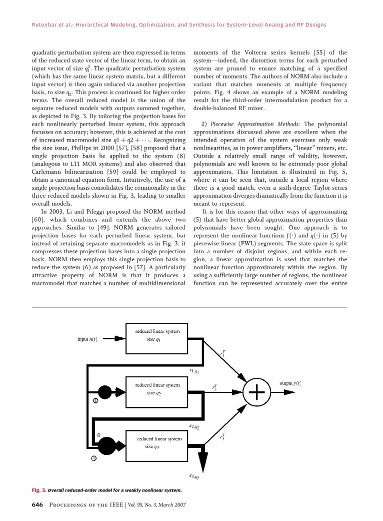
quadratic perturbation system are then expressed in termsof the reduced state vector of the linear term, to obtain an
input vector of size q21 . The quadratic perturbation system
(which has the same linear system matrix, but a different
input vector) is then again reduced via another projection
basis, to size q2. This process is continued for higher order
terms. The overall reduced model is the union of the
separate reduced models with outputs summed together,
as depicted in Fig. 3. By tailoring the projection bases foreach nonlinearly perturbed linear system, this approach
focusses on accuracy; however, this is achieved at the cost
of increased macromodel size q1 þ q2 þ � � �. Recognizing
the size issue, Phillips in 2000 [57], [58] proposed that a
single projection basis be applied to the system (8)
(analogous to LTI MOR systems) and also observed that
Carlemann bilinearization [59] could be employed to
obtain a canonical equation form. Intuitively, the use of asingle projection basis consolidates the commonality in the
three reduced models shown in Fig. 3, leading to smaller
overall models.
In 2003, Li and Pileggi proposed the NORM method
[60], which combines and extends the above two
approaches. Similar to [49], NORM generates tailored
projection bases for each perturbed linear system, but
instead of retaining separate macromodels as in Fig. 3, itcompresses these projection bases into a single projection
basis. NORM then employs this single projection basis to
reduce the system (6) as proposed in [57]. A particularly
attractive property of NORM is that it produces a
macromodel that matches a number of multidimensional
moments of the Volterra series kernels [55] of thesystemVindeed, the distortion terms for each perturbed
system are pruned to ensure matching of a specified
number of moments. The authors of NORM also include a
variant that matches moments at multiple frequency
points. Fig. 4 shows an example of a NORM modeling
result for the third-order intermodulation product for a
double-balanced RF mixer.
2) Piecewise Approximation Methods: The polynomial
approximations discussed above are excellent when the
intended operation of the system exercises only weak
nonlinearities, as in power amplifiers, Blinear[ mixers, etc.
Outside a relatively small range of validity, however,
polynomials are well known to be extremely poor global
approximators. This limitation is illustrated in Fig. 5,
where it can be seen that, outside a local region wherethere is a good match, even a sixth-degree Taylor-series
approximation diverges dramatically from the function it is
meant to represent.
It is for this reason that other ways of approximating
(5) that have better global approximation properties than
polynomials have been sought. One approach is to
represent the nonlinear functions fð�Þ and qð�Þ in (5) by
piecewise linear (PWL) segments. The state space is splitinto a number of disjoint regions, and within each re-
gion, a linear approximation is used that matches the
nonlinear function approximately within the region. By
using a sufficiently large number of regions, the nonlinear
function can be represented accurately over the entire
Fig. 3. Overall reduced-order model for a weakly nonlinear system.
Rutenbar et al.: Hierarchical Modeling, Optimization, and Synthesis for System-Level Analog and RF Designs
646 Proceedings of the IEEE | Vol. 95, No. 3, March 2007

domain of interest. From a macromodeling perspective,
the motivation for PWL approximations is that since the
system is linear within each region, linear macromodeling
methods can be leveraged.
Piecewise linear approximations are not new in circuit
simulation, having been employed in the past mostnotably in attempts to solve the dc operating point
problem [61], [62]. One concern with these methods is a
potential exponential explosion in the number of regions
as the dimension of the state space grows. This is espe-
cially the case when each elemental device within the
circuit is first represented in piecewise form, and the
system of circuit equations is constructed from these
piecewise elements. A combinatorial growth of polytoperegions results via cross-products of the hyperplanes that
demarcate piecewise regions within individual devices. To
circumvent the explosion of regions, which would
severely limit the simplicity of a small macromodel,
Rewienski and White proposed the Trajectory PWL
method (TPWL) [63] in 2001. In TPWL, a reasonable
number of Bcenter points[ is first selected along a
simulation trajectory in the state space, generated by
exciting the circuit with a representative training input.
Around each center point, system nonlinearities are
approximated by linearization, with the region of validityof the linearization defined implicitly, as consisting of all
points that are closer to the given center point than to any
other. Thus, there are only as many piecewise regions as
center points, and combinatorial explosion resulting from
intersections of hyperplanes is avoided. The implicit
piecewise regions in TPWL are in fact identical to the
Voronoi regions defined by the collection of center points
chosen. Within each piecewise region, the TPWLapproach simply reduces the linear system using existing
LTI MOR methods to obtain a reduced linear model. The
reduced linear models of all the piecewise regions are
finally stitched together using a scalar weight function to
form a single-piece reduced model. The weight function
identifies, using a closest-distance metric, whether a test
point in the state space is within a particular piecewise
region and weighs the corresponding reduced linearsystem appropriately.
The TPWL method, by virtue of its use of inherently
better PWL global approximation, avoids the blow-up that
occurs when polynomial-based methods are used with
large inputs. It is thus better suited for circuits with strong
nonlinearities, such as comparators, digital gates, etc.
However, because PWL approximations do not capture
higher order derivative information, TPWL’s ability toreproduce small-signal distortion or intermodulation is
limited.
To address this limitation, Dong and Roychowdhury
proposed a piecewise polynomial (PWP) extension [64] of
TPWL in 2003. PWP combines weakly nonlinear MOR
techniques with the piecewise idea, by approximating the
nonlinear function in each piecewise region by a
polynomial, rather than a purely linear, Taylor expansion.Each piecewise polynomial region is reduced using one of
the polynomial MOR methods outlined above, and theFig. 5. Limitations of global polynomial approximations.
Fig. 4. NORM [60] modeling example. Double-balanced mixed (left) with extracted model for third-order intermodulation
product (middle and right). Example shows a maximum error of 8% over all RF frequencies.
Rutenbar et al. : Hierarchical Modeling, Optimization, and Synthesis for System-Level Analog and RF Designs
Vol. 95, No. 3, March 2007 | Proceedings of the IEEE 647

resulting polynomial reduced models are stitched together
with a scalar weight function, similar to TPWL. Thanks to
its piecewise nature, PWP is able to handle strong
nonlinearities globally; because of its use of local Taylorexpansions in each region, it is also able to capture small-
signal distortion and intermodulation well. Thus, PWP
expands the scope of applicability of nonlinear macro-
modeling to encompass blocks in which strong and weak
nonlinearities both play an important functional role.
PWP is illustrated using the fully differential op-amp
shown in Fig. 6. The circuit comprises 50 MOSFETs and
39 nodes. It was designed to provide about 70 dB of dcgain, with a slew rate of 20 V=�s and an open-loop 3-dB-
bandwidth of f 0 � 10 kHz. The PWP-generated macro-
model was of size 19, a number that refers to the size of the
differential equation system describing the macromodel
(i.e., roughly analogous to the number of nodes in the
circuit). The macromodel is compared against the full
SPICE-level op-amp using a number of analyses and
performance metrics, representative of actual use in a real
industrial design flow. Fig. 7 shows the results ofperforming dc sweep analyses of both the original circuit
and the PWP-generated macromodel. Note the excellent
match. Fig. 8 compares Bode plots obtained by ac analysis;
two ac sweeps, obtained at different dc bias points, are
shown. Note that PWP provides excellent matches around
each bias point.
If the op-amp is used as a linear amplifier with small
inputs, distortion and intermodulation are importantperformance metrics. As mentioned earlier, one of the
strengths of PWP-generated macromodels is that weak
nonlinearities, responsible for distortion and intermodu-
lation, are captured well. Such weakly nonlinear effects are
best simulated using frequency-domain harmonic balance
(HB) analysis, for which we choose the one-tone sinusoidal
input V in1 � V in2 ¼ A sinð2� 100tÞ and Cload ¼ 10 pF.
The input magnitude A is swept over several decades andthe first two harmonics plotted in Fig. 9. It can be seen that
for the entire input range, there is an excellent match of
the distortion component from the macromodel versus
that of the full circuit. Note that the same macromodel is
used for this harmonic balance simulation as for all the
other analyses presented. Speedups of about 8.1 were
obtained compared to the harmonic balance simulations.
Another strength of PWP is that it can capture theeffects of strong nonlinearities excited by large-signal
swings. To demonstrate this, a transient analysis was run
with a large, rapidly rising input; the resulting waveforms
are shown in Fig. 10. The slope of the input was chosen to
excite slew-rate limiting, a dynamical phenomenon caused
by strong nonlinearities (saturation of differential ampli-
fier structures). Note the excellent match between the
original circuit and the macromodel. The macromodel-based simulation ran about 8 faster.
Unfortunately, two problems are shared by all the
piecewise trajectory-based modeling techniques, both the
Fig. 6. Current-mirror op-amp with 50 MOSFETs and 39 nodes.
Fig. 7. DC sweep of op-amp from Fig. 6.
Rutenbar et al.: Hierarchical Modeling, Optimization, and Synthesis for System-Level Analog and RF Designs
648 Proceedings of the IEEE | Vol. 95, No. 3, March 2007

original TPWL linear form [63] and the generalized
quadratic PWP extension of [64]. As noted in Tiwary and
Rutenbar [85], all the trajectory methods are fragile in the
face of insufficient training waveforms to build the
essential trajectory Bcoverage[ of the state space. One
can remedy this with a more rigorous training regime, of
course. However, this creates a new problem: simulationinefficiency. Trajectory models interpolate from all the
visited linearizations to estimate the behavior at any new
point in the state space. Curing the undertraining problem
can easily increase the number of trajectory samples from
tens or hundreds to 10 000 or more and destroy any
simulation speedup gains we sought to achieve. The same
authors demonstrate a solution, the so-called scalabletrajectory model [85]. Using ideas from data mining, they
show how to cluster trajectory linearizations in the state
space, prune away redundant linearizations, and synthe-
size estimated linearizations to represent each cluster of
similar points. Then, instead of interpolating based on all
visited trajectory points, they use a fast high-dimensional
nearest neighbor lookup strategy in the trajectory space to
select only the Brelevant[ linearizations to use to predictthe local dynamics. The strategy allows the designer to
train the model with a wide variety of potentially useful
waveforms but enables the model to interpolate from a
minimal set of the most locally relevant linearizations,
preserving most of the speedup gains we originally sought.
Fig. 11 shows an example from [85] of a simple common-
mode feedback (CMFB) op-amp replaced in a sample-and-
hold amplifier context with a scalable trajectory model.
Fig. 8. AC analysis of op-amp from Fig. 6: (left) AC sweep (at common-mode dc bias 2.5 V) and (right) AC sweep
(at common-mode dc bias 2.0 V).
Fig. 9. Harmonic analysis of current-mirror op-amp: full op-amp
(solid line) and PWP model (discrete points).
Fig. 10. Transient analysis of current-mirror op-amp with
fast step input.
Rutenbar et al. : Hierarchical Modeling, Optimization, and Synthesis for System-Level Analog and RF Designs
Vol. 95, No. 3, March 2007 | Proceedings of the IEEE 649

Additional work on the scalable model [86] showed how to
output loading effects and apply additional model-order
reductions to obtain faster models which can be success-
fully reinserted in an arbitrary system-level design.
D. Macromodeling Oscillatory SystemsOscillators are ubiquitous in electronic systems. They
generate periodic signals, typically sinusoidal or square-
like waveforms, that are used for a variety of purposes.
From the standpoint of both simulation and macromodel-
ing, oscillators present special challenges. Traditional
circuit simulators such as SPICE [65], [66] consumesignificant computer time to simulate the transient
behavior of oscillators. As a result, specialized techniques
based on using phase macromodels (e.g., [67]–[76]) have
been developed for the simulation of oscillator-based
systems. The most basic class of phase macromodelsassumes a linear relationship between input perturbations
and the output phase of an oscillator. A general time-
varying expression for the phase �ðtÞ can be given by
�ðtÞ ¼Xn
k¼1
Z1�1
hk�ðt; �Þikð�Þd�: (8)
Fig. 11. Example of scalable trajectory model from [85]. (a) CMFB op-amp with 40 MOSFETs, 24 nodes. (b) SPICE versus model
accuracy for a scalable trajectory model of CMFB op-amp, hierarchically reinserted into sample-and-hold design.
Rutenbar et al.: Hierarchical Modeling, Optimization, and Synthesis for System-Level Analog and RF Designs
650 Proceedings of the IEEE | Vol. 95, No. 3, March 2007

The summation is over all perturbations ik to thecircuit; hk
�ðt; �Þ denotes a time-varying impulse response
to the kth noise source. Very frequently, time-invariant
simplifications of (8) are employed [77]. Linear models
suffer, however, from a number of important deficiencies.
In particular, they have been shown to be inadequate for
capturing fundamentally nonlinear effects such as injec-
tion locking [82]. As a result, automatically extracted
nonlinear phase models have recently been proposed[78], [79], [82]–[84] that are considerably more accurate
than linear ones. The nonlinear phase macromodel has
the form
_�ðtÞ ¼ vT1 t þ �ðtÞð Þ � bðtÞ: (9)
In the above equation, v1ðtÞ is called the perturbation
projection vector (PPV) [79]; it is a periodic vector
function of time, with the same period as that of the
unperturbed oscillator. A key difference between thenonlinear phase model (9) and traditional linear phase
models is the inclusion of the phase shift �ðtÞ inside the
perturbation projection vector v1ðtÞ. �ðtÞ in the nonlinear
phase model has units of time; the equivalent phase shift,
in radians, can be obtained by multiplying �ðtÞ by the free-
running oscillation frequency !0.
We illustrate the use of (9) by applying it to model the
VCO inside a simple PLL [80], shown in block form inFig. 12. Using the nonlinear macromodel (9), we simulate
the transient behavior of the PLL and compare the results
with a full simulation and with linear models. The
simulations encompass several important effects, includ-
ing static phase offset, step response, and cycle slipping.
Fig. 13 depicts the static phase offset of the PLL when a
reference signal of the same frequency as the VCO’s free-
running frequency is applied. The PLL is simulated tolocked steady state and the phase difference between the
reference and the VCO output is shown. The fact that the
LPF is not a perfect one results in high-frequency ac
components being fed to the VCO, affecting its static phase
offset. Observe that both the full simulation and the
nonlinear macromodel (9) predict identical static phase
offsets of about 0.43 radians. Note also that the linear
phase macromodel fails to capture this correctly, reporting
a static phase offset of 0.
Fig. 14 depicts the step response of the PLL at differentreference frequencies. Fig. 14(a) shows the step responses
using the full simulation, the linear phase model, and the
nonlinear macromodel when the reference frequency is
1:07f 0. With this reference signal, both the linear and
nonlinear macromodels track the reference frequency
well, although, as expected, the nonlinear model provides
a more accurate simulation than the linear one. When the
reference frequency is increased to 1:074f 0, however, thelinear phase macromodel is unable to track the reference
correctly, as shown in Fig. 14(b). However, the nonlinear
macromodel remains accurate. The breakdown of the
linear model is even more apparent when the reference
frequency is increased to 1:083f 0, at which the PLL is
unable to achieve stable lock, as shown in Fig. 14(c). Note
that the nonlinear macromodel remains accurate.
Finally, Fig. 15 illustrates the prediction of cycleslipping. A reference frequency f ref ¼ 1:07f 0 is provided
and the PLL is brought to locked steady state. When a
sinusoidal perturbation with amplitude 5 mA and duration
10 VCO periods is injected, the PLL loses lock. As shown in
Fig. 15(a), the phase difference between the reference
signal and the VCO output slips over many VCO cycles,
until finally, lock is reachieved with a phase shift of �2�.
Both nonlinear and linear macromodels predict thequalitative phenomenon correctly in this case, with the
nonlinear macromodel matching the full simulation better
than the linear one. When the injection amplitude is
reduced to 3 mA, however, as shown in Fig. 15(b), the
linear macromodel fails, still predicting a cycle slip. In
reality, the PLL is able to recover without slipping a cycle,
as predicted by both the nonlinear macromodel and the
full simulation.Fig. 12. Functional block diagram of PLL.
Fig. 13. PLL static phase offset when fref ¼ f0.
Rutenbar et al. : Hierarchical Modeling, Optimization, and Synthesis for System-Level Analog and RF Designs
Vol. 95, No. 3, March 2007 | Proceedings of the IEEE 651

E. Nonlinear Macromodelling: Current andFuture Applicability
It should be noted that the problem of extracting
nonlinear macromodels by algorithm is a very difficult
problem. However, for future design sustainability, it is of
great importance to solve this problem in practically useful
ways. Of the methods surveyed above, the techniques for
nonlinear oscillator macromodelling are the most matureat this pointVthe extraction techniques involved are being
adopted by a number of CAD and semiconductor
companies. The weakly nonlinear macromodelling meth-
ods discussed above are the most specialized, whereas the
trajectory-piecewise strongly nonlinear macromodelling
methods are perhaps the most broadly applicable. How-
ever, they are also, as already noted above, the most
heuristically based technique of the three; it is expectedthat considerably more research will be required before
these techniques achieve the reliability and robustness
necessary for broad industrial deployment.
III . HIERARCHICAL SYNTHESISTECHNIQUES
Recent years have seen the emergence of commercial CAD
tool support for analog cell-level circuit and layoutsynthesis. Gielen and Rutenbar [2] offer a fairly complete
survey of the area. Analog synthesis consists of two major
steps: 1) circuit synthesis followed by 2) layout synthesis.
Most of the basic techniques in both circuit and layout
synthesis rely on powerful numerical optimization engines
coupled to Bevaluation engines[ that qualify the merit of
some evolving analog circuit or layout candidate. Fig. 16
shows the basic flow of most current tools. The goal ofanalog circuit synthesis is to create a sized circuit
Fig. 14. Step response of PLL model with varying values of fref. (a) Response with fref ¼ 1:07f0. (b) Response with fref ¼ 1:074f0.
(c) Response with fref ¼ 1:083f0.
Rutenbar et al.: Hierarchical Modeling, Optimization, and Synthesis for System-Level Analog and RF Designs
652 Proceedings of the IEEE | Vol. 95, No. 3, March 2007

schematic from given circuit specifications. It is a difficultand critical step for several reasons: 1) most analog circuits
require a custom optimized design; 2) the design problem
is typically underconstrained with many degrees of
freedom; and 3) it is common that many (often
conflicting) performance requirements must to be taken
into account, and tradeoffs must be made that satisfy the
designer using these tools.
We focus in this paper on the circuit, rather than layoutsynthesis. The former is a numerical problem that relies
heavily on the macromodeling ideas of the previous
section; the latter relies more on combinatorial optimiza-
tion techniques (see [3]). Given a circuit schematic and the
circuit’s performance specifications, the sizes and biasing
of all devices have to be determined such that the circuit
meets the specifications at some optimal cost. It is the
optimization engine that determines these optimal values,while the evaluation engine assesses the performance. In
many cases, the initial sizing produces a near-optimal
design that is further fine-tuned with a circuit optimization
tool, e.g., to improve yield and design robustness. The
performance of the resulting design is then verified using
detailed circuit simulations with a simulator such as SPICE.
Although successful, these simulation-based circuit
optimization methods still have to be used with care bydesigners because the run times (and therefore also the
initial debug time) may still be long, especially since the
optimizer may produce improper designs if the right
design constraints are not added to the optimization
problem. Reducing the CPU time, and the complexities of
specifying the best set of design constraints, are active
areas of research.
The flow of Fig. 16 presents several challenges whenwe try to scale these ideas from circuits to systems.
Simulation-based synthesis (e.g., [87]–[90]) uses efficient
numerical optimization to visit many circuit candidates
and fully evaluates each candidate via detailed simulation.
This methodology works very well for circuits having in the
range of a few hundred devices. However, for larger
circuits, the simulation time required for a single
simulation is too large to do a practical simulator-in-the-loop circuit sizing. Also, due to the curse of dimension-
ality, the design space in which to search for optimal
design points becomes too large for these circuits to be
handled by these Bflat[ optimization-based tools.
We survey approaches to handling these larger system-
level problems in this section. Targeting the explicitly
hierarchical structure of these designs is of critical
importance. Macromodeling also plays a central role, butit is perhaps surprising that the performance-oriented
techniques of the previous section are a necessary but not
yet sufficient response to these problems. In particular, we
need a different sort of modeling abstraction, which builds
parameterized tradeoff models, of the circuit components,
for use in system-level analysis and synthesis.
A. Macromodeling RevisitedOne might be tempted to believe that the only problem
with the optimization-based flow of Fig. 16 is the
burdensome CPU time needed to evaluate each proposed
solution candidate, since it relies on full device-level
simulation for maximum fidelity and flexibility [87]. Thus,
replacing some or all of the circuit level components with
appropriate macromodels seems a good solution strategy.
If we can make the necessary simulation evaluations runsufficiently fast, perhaps we can use these Bflat[ synthesis
strategies without additional modification.
Unfortunately, the Binstance oriented[ model extrac-
tion techniques of Section II are a necessary but not
sufficient solution to this problem. Let us consider a
concrete example to explain the problem. Suppose we
want to synthesize device-level sizing/biasing for a PLL.
Fig. 15. Cycle slipping of PLL model for different noise amplitudes.
(a) PLL cycle slipping, for a noise amplitude of 5 mA. (b) PLL
cycle slipping, for a noise amplitude of 3 mA.
Rutenbar et al. : Hierarchical Modeling, Optimization, and Synthesis for System-Level Analog and RF Designs
Vol. 95, No. 3, March 2007 | Proceedings of the IEEE 653
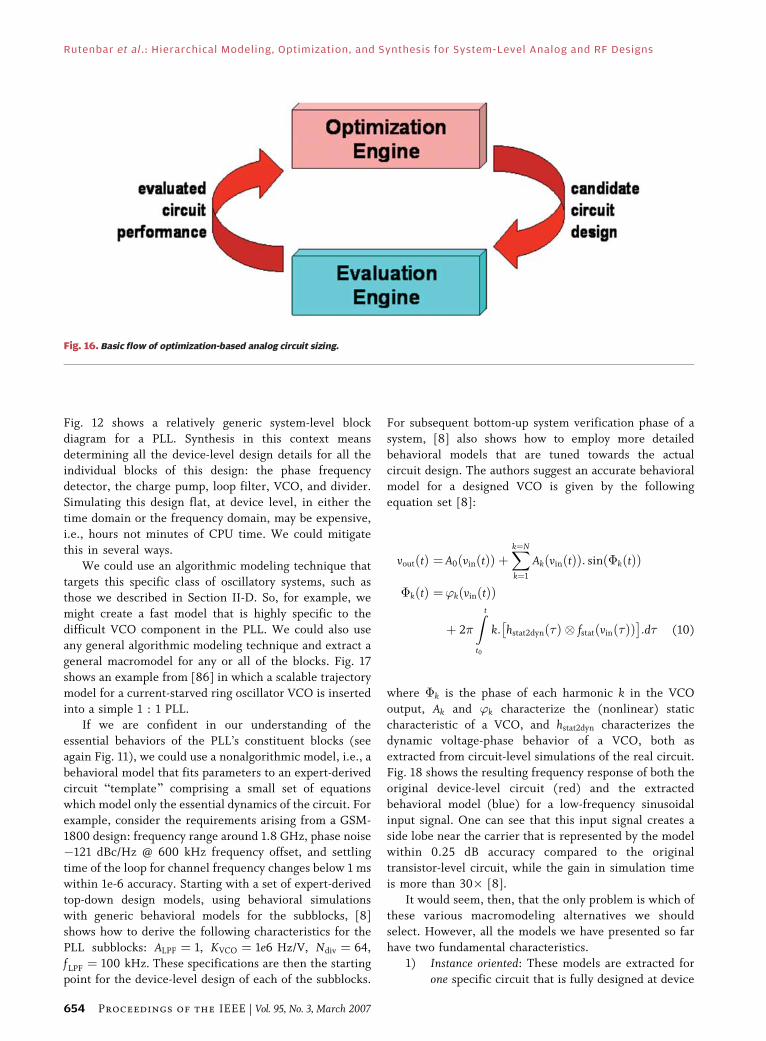
Fig. 12 shows a relatively generic system-level block
diagram for a PLL. Synthesis in this context means
determining all the device-level design details for all theindividual blocks of this design: the phase frequency
detector, the charge pump, loop filter, VCO, and divider.
Simulating this design flat, at device level, in either the
time domain or the frequency domain, may be expensive,
i.e., hours not minutes of CPU time. We could mitigate
this in several ways.
We could use an algorithmic modeling technique that
targets this specific class of oscillatory systems, such asthose we described in Section II-D. So, for example, we
might create a fast model that is highly specific to the
difficult VCO component in the PLL. We could also use
any general algorithmic modeling technique and extract a
general macromodel for any or all of the blocks. Fig. 17
shows an example from [86] in which a scalable trajectory
model for a current-starved ring oscillator VCO is inserted
into a simple 1 : 1 PLL.If we are confident in our understanding of the
essential behaviors of the PLL’s constituent blocks (see
again Fig. 11), we could use a nonalgorithmic model, i.e., a
behavioral model that fits parameters to an expert-derived
circuit Btemplate[ comprising a small set of equations
which model only the essential dynamics of the circuit. For
example, consider the requirements arising from a GSM-
1800 design: frequency range around 1.8 GHz, phase noise�121 dBc/Hz @ 600 kHz frequency offset, and settling
time of the loop for channel frequency changes below 1 ms
within 1e-6 accuracy. Starting with a set of expert-derived
top-down design models, using behavioral simulations
with generic behavioral models for the subblocks, [8]
shows how to derive the following characteristics for the
PLL subblocks: ALPF ¼ 1, KVCO ¼ 1e6 Hz/V, Ndiv ¼ 64,
f LPF ¼ 100 kHz. These specifications are then the startingpoint for the device-level design of each of the subblocks.
For subsequent bottom-up system verification phase of a
system, [8] also shows how to employ more detailed
behavioral models that are tuned towards the actualcircuit design. The authors suggest an accurate behavioral
model for a designed VCO is given by the following
equation set [8]:
voutðtÞ ¼ A0 vinðtÞð Þ þXk¼N
k¼1
Ak vinðtÞð Þ: sin �kðtÞð Þ
�kðtÞ ¼’k vinðtÞð Þ
þ 2�
Z t
t0
k: hstat2dynð�Þ � fstat vinð�Þð Þ
:d� (10)
where �k is the phase of each harmonic k in the VCO
output, Ak and ’k characterize the (nonlinear) static
characteristic of a VCO, and hstat2dyn characterizes thedynamic voltage-phase behavior of a VCO, both as
extracted from circuit-level simulations of the real circuit.
Fig. 18 shows the resulting frequency response of both the
original device-level circuit (red) and the extracted
behavioral model (blue) for a low-frequency sinusoidal
input signal. One can see that this input signal creates a
side lobe near the carrier that is represented by the model
within 0.25 dB accuracy compared to the originaltransistor-level circuit, while the gain in simulation time
is more than 30 [8].
It would seem, then, that the only problem is which of
these various macromodeling alternatives we should
select. However, all the models we have presented so far
have two fundamental characteristics.
1) Instance oriented: These models are extracted for
one specific circuit that is fully designed at device
Fig. 16. Basic flow of optimization-based analog circuit sizing.
Rutenbar et al.: Hierarchical Modeling, Optimization, and Synthesis for System-Level Analog and RF Designs
654 Proceedings of the IEEE | Vol. 95, No. 3, March 2007

level. If we change any of the device-level designvariables, we must re-extract the model, which
may be costly.
2) Verification-oriented: These instance-specific mod-
els are intended to be used in scenarios where we
can amortize the cost of constructing the model
over a large number of simulation runs that will be
used to verify the correctness of the system-level
design assembled from these models.For synthesis tasks in which we plan to visit a large
number of intermediate circuit design configurations, we
really want a parameterized macromodel. This means amodel that predicts the behavior of the circuit as a
function of its designable parameters, e.g., transistor
widths, lengths, biasing, etc. Since this is a much more
challenging problem than extracting an instance-specific
model, we usually are willing to accept some loss of model
fidelity. For example, we may be willing to ignore some
secondary or tertiary effects at this level, focus only on the
essential nonidealities, and strive to repair these omissionswhen we do detailed circuit-level synthesis later, for each
circuit.
Fig. 17. Replacing the VCO in simple 1 : 1 PLL with scalable trajectory model. (a) Simple 1 : 1 PLL architecture with a current-starved
ring-oscillator VCO (highlighted in bold). (b) SPICE versus scalable trajectory model simulation results; figure shows
transient simulation result for PLL going into lock.
Rutenbar et al. : Hierarchical Modeling, Optimization, and Synthesis for System-Level Analog and RF Designs
Vol. 95, No. 3, March 2007 | Proceedings of the IEEE 655

B. Parametric Circuit PerformanceModeling Techniques
Parametric performance modelsVin contrast to the
instance models described in earlier sectionsVrelate the
achievable performances of a circuit (e.g., gain, band-
width, slew rate, or phase margin) to its design variables
(e.g., device sizes and biasing). These are also sometimescalled performance space or design space models. Fig. 19 for
example shows part of such a parametric model, displaying
the phase margin as a function of two design variables for a
CMOS operational amplifier [9], [10]. Such performance
models are used to speed up circuit sizing: in every
iteration of the synthesis procedure of Fig. 16, calls to the
transistor-level simulator are replaced by evaluations of asuitable constructed parametric model. This not only
results in substantial speedups, once the performance
models have been created and calibrated, but in many
cases is the difference between a tractable and an
intractable system-level synthesis process. The model
building process is a one-time up-front investment that
has to be done only once for each circuit in each
technology.Most approaches for performance model generation
are based on fitting or regression methods where the
coeffients of a prespecified modelVoften referred to as a
model templateVare fitted to have the model match as
closely as possible a sample set of simulated data points. As
a concrete example, consider the flow of Fig. 20. First, a
large set of data samples is generated by simulating well
chosen design points with SPICE. For instance, a design-of-experiments (DOE) scheme can be used to sample the
design space. The use of SPICE simulations allows the
modeling of any nonlinear circuits and circuit character-
istics, as opposed to symbolic analysis techniques that are
restricted to rather linear circuit characteristics only. Next,
a model is fitted through these data points. If the modeling
error is too large, then additional data points can be
generated, or a more sophisticated model template has tobe chosen.
A recent example of such a fitting approach is the
automatic generation of posynomial performance models
for analog circuits, that are created by fitting a pre-
assumed posynomial equation template to simulation data
created according to a design of experiments scheme [9].
Such a posynomial model could then, for instance, be used
in the very efficient sizing of analog circuits throughconvex circuit optimization.
Fig. 18. Frequency response of an extracted behavioral VCO model
(blue) compared to the underlying device-level circuit
response (red) [8].
Fig. 19. High-speed CMOS OTA (left) and performance model of phase margin as a function of two design variables (right).
Note that this is just a subset of the actual multidimensional parametric performance model.
Rutenbar et al.: Hierarchical Modeling, Optimization, and Synthesis for System-Level Analog and RF Designs
656 Proceedings of the IEEE | Vol. 95, No. 3, March 2007

One of the core problems with all regression style
parameterized models is the need to balance the goodness-
of-fit of the model against the complexity (i.e., numerical
difficulty) of fitting the template coefficients necessary to
complete the model. For example, a linear model of the
circuit response is quite easy to fit, even for many
independent variables. But, unless we really expect the
behavior to be linear, it will likely be a poor fit to thecircuit’s actual behavior. The quadratic style posynomial
models of [9] are one response to this problem. This
particular model offers a wider range of nonlinearity, along
with a workable heuristic, to calculate numerically the
essential fitting parameters. The work in [91] takes this a
step further and develops a very efficient fitting strategy for
models of this type. One problem with higher dimensional
nonlinear templates is that they create numerically
challenging problems to solve for all the necessary fittingcoefficients. Both [9] and [91] use a quadratic performance
template for circuit performance fðXÞ
fðXÞ ¼ XTAX þ BTX þ C (11)
where X ¼ ½x1 � � � xN�T is the vector of designable circuit
parameters, A is an N N matrix of coefficients, B is a
N-vector of unknown coefficients, and C is a single
unknown scalar coefficient. Our goal is find A, B, and C so
that the quadratic function of vector X closely matches a
large set of training data, e.g., sampled from many SPICE
simulations. For large N, i.e., for a design with manydegrees of freedom, we have OðN2Þ coefficients to solve
for, which can be daunting. The methodology in [91],
called ROAD, replaces the large unknown A matrix with a
carefully chosen low-rank approximation; the technique
employs the rank-one projection which can be solved for
numerically via an efficient, implicit power iteration in
OðNÞ steps. Fig. 21 shows one example of parametric
fitting using ROAD.Another class of regression techniques borrows ideas
from data mining, which focuses on extracting meaningful
patterns (e.g., fitting predictive models) to large amounts
of high-dimensional data (e.g., training a model by means
of many SPICE runs). There is a range of useful techniques
from this domain. One of the first large-scale applications
of these ideas is the work of Liu et al. in [11]. A perennial
problem in the area of parametric modeling is how onechooses the nonlinear template to which one will try to fit
the desired circuit behavior. References [9] and [91]
choose an explicit analytical form, a higher order quadratic
of (11). Reference [11] supports fitting to a more nonlinear
form by using a so-called boosted community of regressors.
The idea is to iteratively fit a sequence of regression
Fig. 20. Flow for template-based and template-free
performance modeling.
Fig. 21. Applying ROAD [91] projection-based quadratic fitting procedure to 0.25-�m CMOS op-amp. Results show that
low-rank approximation strategy is extremely accurate and also reduces fitting complexity from OðN2Þ to OðNÞ.
Rutenbar et al. : Hierarchical Modeling, Optimization, and Synthesis for System-Level Analog and RF Designs
Vol. 95, No. 3, March 2007 | Proceedings of the IEEE 657
models; later models in the sequence fit well in regions of
the design space where earlier models fit poorly. An
elegant numerical formulation, called boosting [93],
efficiently combines the predictions of the many individ-
ual models into a single final numerical value. Thetechnique has the attractive feature that any specific
nonlinear regressor may be used in the overall fitting
process; Liu et al. used a set of relatively small neural
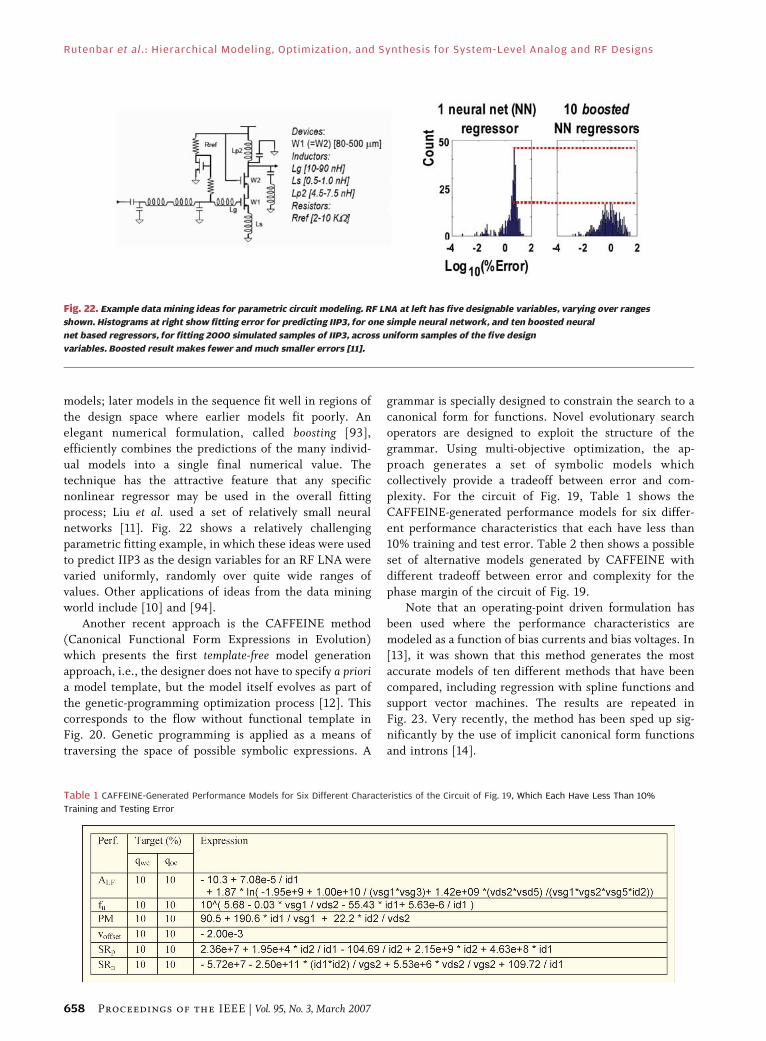
networks [11]. Fig. 22 shows a relatively challenging
parametric fitting example, in which these ideas were used
to predict IIP3 as the design variables for an RF LNA were
varied uniformly, randomly over quite wide ranges of
values. Other applications of ideas from the data miningworld include [10] and [94].
Another recent approach is the CAFFEINE method
(Canonical Functional Form Expressions in Evolution)
which presents the first template-free model generation
approach, i.e., the designer does not have to specify a prioria model template, but the model itself evolves as part of
the genetic-programming optimization process [12]. This
corresponds to the flow without functional template inFig. 20. Genetic programming is applied as a means of
traversing the space of possible symbolic expressions. A
grammar is specially designed to constrain the search to a
canonical form for functions. Novel evolutionary search
operators are designed to exploit the structure of the
grammar. Using multi-objective optimization, the ap-
proach generates a set of symbolic models whichcollectively provide a tradeoff between error and com-
plexity. For the circuit of Fig. 19, Table 1 shows the
CAFFEINE-generated performance models for six differ-
ent performance characteristics that each have less than
10% training and test error. Table 2 then shows a possible
set of alternative models generated by CAFFEINE with
different tradeoff between error and complexity for the
phase margin of the circuit of Fig. 19.Note that an operating-point driven formulation has
been used where the performance characteristics are
modeled as a function of bias currents and bias voltages. In
[13], it was shown that this method generates the most
accurate models of ten different methods that have been
compared, including regression with spline functions and
support vector machines. The results are repeated in
Fig. 23. Very recently, the method has been sped up sig-nificantly by the use of implicit canonical form functions
and introns [14].
Fig. 22. Example data mining ideas for parametric circuit modeling. RF LNA at left has five designable variables, varying over ranges
shown. Histograms at right show fitting error for predicting IIP3, for one simple neural network, and ten boosted neural
net based regressors, for fitting 2000 simulated samples of IIP3, across uniform samples of the five design
variables. Boosted result makes fewer and much smaller errors [11].
Table 1 CAFFEINE-Generated Performance Models for Six Different Characteristics of the Circuit of Fig. 19, Which Each Have Less Than 10%
Training and Testing Error
Rutenbar et al.: Hierarchical Modeling, Optimization, and Synthesis for System-Level Analog and RF Designs
658 Proceedings of the IEEE | Vol. 95, No. 3, March 2007

A final class of important parametric modeling tech-
nique are the Pareto methods [4], [5], [95], [96]. We briefly
review the fundamental idea of Pareto optimality, following
the discussion of [97]. The capability of any analog circuit is
defined using a set of performance metrics (e.g., dc gain,
bandwidth, power, slew rate for an operational amplifier).
Like any physical system, there are limits on how good
these metrics can be for any circuit topology. The set of allpossible performance metric values achievable by any
circuit topology defines the performance feasibility region of
the topology. These performance metrics are often
competing (e.g., gain and bandwidth), and certain portions
of the feasible region boundary define the tradeoff
relationship while trying to achieve the optimal values for
these metrics. These tradeoff surfaces are said to be Paretooptimal. These are referred to equivalently as Pareto curves,Pareto fronts, and Pareto tradeoffs.
Suppose that x 2 X � Rn is the vector of n design
variables. pðxÞ 2 P � Rm is the vector of circuit perfor-
mances. These performances can be categorized into
constrained performances pc (which must meet certain
specifications for acceptable circuit performance) and
objective performances po (which are to be optimized: we
assume minimized without loss of generality).
cðxÞ 2 C � Rl is the vector of constraint variables that
are needed to guarantee correct circuit operation.
gðc;pcÞ 2 F is the vector of real-valued constraintfunctions to guarantee correct circuit behavior and
minimum acceptable performance ðg � 0Þ. These include
constraints like minimum UGF specification, dc biasing
conditions, etc.
The performance feasibility region of a circuit is the
subset of P over which the constraints g are met. Here, we
define the domination operator (a dominates b)
a � b , 8i21;...;kai � bi ^ 9i21;...;kai G bi: (12)
Fig. 23. Comparison of accumulated modeling error for six different performance characteristics of circuit of Fig. 19 for ten
different performance modeling methods, starting from the same original set of SPICE data points.
Table 2 CAFFEINE-Generated Performance Models of Phase Margin (PM), in Order of Decreasing Error and Increasing Complexity, for the
Circuit of Fig. 19
Rutenbar et al. : Hierarchical Modeling, Optimization, and Synthesis for System-Level Analog and RF Designs
Vol. 95, No. 3, March 2007 | Proceedings of the IEEE 659

The Pareto-optimal front is the set of points on thefeasible region boundary that are not dominated by any
other point in the feasible region. Computing the
performance feasibility region of a circuit topology will
imply computing the set of Bbest[ possible points in terms
of the objective performances and this is the Pareto-
optimal front. This front defines the capability limit of the
topology in terms of the objective performance metrics,
assuming all the constraints g are met.The Pareto-optimal front generation problem can be
formulated as the following multi-objective optimization
problem:
Minimize poðxÞ ¼ po1ðxÞ; po2ðxÞ; . . . ; pokðxÞf gs:t: g cðxÞ;pcðxÞð Þ � 0;x 2 X: (13)
A multi-objective optimization algorithm to solve this
problem will generate points on the Pareto-optimal front,
while satisfying two requirements. First, the solution set
should approximate the real Pareto front as closely as
possible and the algorithm should generate the solution set
as quickly as possible. Second, the solution points should
be uniformly spread out over a large extent of the Pareto
front. This is to enable reliable model building.There are several approaches to generating the Pareto
front. An interesting characteristic of all such techniques is
that they leverage the core infrastructure of existing
circuit-level analog synthesis tools. In other words, one can
extend the engines that synthesize sizing/biasing for an
individual circuit with a specific set of performance targets
and use these instead to trace out the Pareto front. For
example, stochastic approaches such as the Watson tool [4]
exploit ideas from genetic algorithms and try to evolvepopulations of sized circuits whose Bfitness[ is rewarded
proportionally to how well each candidate fill in gaps in
the evolving Pareto front and how Bdominated[ the point
is by other members of the population.It is also possible to use more direct methods to find
these curves. Of these, the Normal Boundary Intersection(NBI) method is most well known [96]. Suppose, viacircuit synthesis, we can find circuits that define the bestpossible values of each individual performance objectivespoðxÞ ¼ fpo1ðxÞ; po2ðxÞ; . . . ; pokðxÞg. Roughly speaking,we build the convex hull of these individual points andthen search in a direction normal to this hull, toward thePareto-optimal points, from a set of suitably uniformlyspaced points on this hull. Fig. 24 illustrates the idea forthe geometrically simplest case of a two-dimensionalPareto front; in this case, the convex hull is simply thechord between the points defining the two best values ofthe two performance objectives. We search from thepoints on the convex chord, adding an additionalconstraint that we seek a circuit solution that: 1) lies onthis normal and 2) is maximally distant from the chord.Such points will comprise the Pareto points we seek. Aversion of the WiCKed synthesis tool uses NBI ideas forautomatically tracing Pareto points [5]. One challengewith this formulation is the need to add the additionalpoints-on-the-normal constraint, which takes the possiblynumerically more difficult form of an equality constraint.It is possible to relax this and formulate an NBI-likemethod using only inequalities, as shown in [95]. Theattractive feature of this version is that the problem ofsearch along the normal is transformed into a problem ofsearch near the normal, which involves only inequalitiesconstraints, which are robustly handled by most industrialsynthesis engines.
Fig. 24. Illustrating NBI method [96] for tracing Pareto front in two dimensions. From individual minima for two performance
objectives (left) the convex hull H (chord, right) of these points is formed, then from the centroid of H
a search on the normal is performed to find the new Pareto point.
Rutenbar et al.: Hierarchical Modeling, Optimization, and Synthesis for System-Level Analog and RF Designs
660 Proceedings of the IEEE | Vol. 95, No. 3, March 2007

Finally, it is worth noting that another significantbenefit of the Pareto-based model is dimensionality
reduction. That is, we replace the potentially large number
of degrees of freedom of a cell-level circuit with the
relatively small number of degrees of freedom of the
Pareto curve. To be concrete, suppose we have an amplifier
which has 20 CMOS devices; we need perhaps 20 widths
and 20 lengths to design this circuit. However, suppose
that at system level, all we really want to know is the bestpoint on the gain versus bandwidth Pareto curve. Then, we
have really reduced this to a single degree of freedom:
when we select a value for one of these dimensions, our
Pareto model uniquely specifies the other. This dimen-
sionality reduction and the fact that these sorts of tradeoff
analyses are extremely familiar to working circuit de-
signers accounts for recent interest in the Pareto models.
Of course, these do become quite unwieldy in more thana few dimensions; this is the main drawback of the
approach.
Despite the progress made so far, still more research in
the area of automatic performance model generation is
needed to reduce analog synthesis times, especially for
hierarchical synthesis of complex analog blocks. The field
is a very active research area at the moment.
C. Hierarchical Synthesis FlowsRecall that our original motivations for the various
forms of modeling in the previous sections were twofold:
first, for full-system design verification, we needed
efficient instance-based macromodels that allowed use to
simulate large designs in tractable amounts of time;
second, for optimization-based synthesis flows which visit
many intermediate circuit solutions and evaluate eachwith full simulation, we needed efficient parametric
models that let us quickly explore how changes circuit-
level changes affect system-level outcomes. In this sec-
tion, we briefly review how synthesis can be organized,
using all these modeling ideas.
The earliest approaches used top-down strategies.
Chang et al. [105], [106] described a constraint-driven
top-down design methodology where constraints arepropagated down the hierarchy for complex mixed-signal
systems. The methodology is demonstrated for some
practical design examples. The performance constraints
are also used to control the layout synthesis tools (place-
ment, routing). A second early approach that can be
mentioned here is the OASYS tool of [6]: at each level in
the design hierarchy, the performance specifications of
the subblocks within the selected block architecture haveto be determined based on the block’s overall specifica-
tions. This can be done in a top-down manner using
optimization methods at each level, until the device level
is reached and all devices have been sized. The complete
design flow is then an alternation of topology selection
(i.e., picking the right circuit-level architecture) and
specification translation (i.e., determining how specifica-
tions at one level decompose into specification at thenext). Reference [6] suggested a set of equation-based
strategies for this purpose.
Unfortunately, hierarchical techniques based on ad hocsets of equations have not proven to be very practical: they
require excessive amounts of effort to redirect for new
circuits and new technologies. One interesting work-
around strategy is to restrict the form of the equations
used to model devices, circuits, and systemVlevelarrangements of blocks. For example, if one restricts all
performance objectives to a posynomial form, one can
apply powerful, efficient convex optimization techniques
to find solutions. These ideas have been applied at circuit
level (e.g., for op-amps [98] and LC oscillators [99]) and
for a few system-level designs (e.g., simple converters
[100] and PLLs [101]). However, the effort to transform
performance goals into the restrictive convex form canitself be challenging, the quality of the fit may be
problematic, and each new circuit requires a new set of
burdensome hand-developed analytical equations.
In light of this, we can see why there is such interest in
parameterized macromodels. These potentially let us keep
the simulator-in-the-loop optimization flow in the style of
Fig. 16 but provide the necessary twin reductions in per-
candidate simulation times and number of degrees offreedom being optimized. Phelps et al. [88] was one no-
table step in this direction who showed how some simple
macromodels for the essential blocks in an industrial
ADSL design could allow simulation-based synthesis to be
performed. The experiment showed how to resynthesize a
multiple-week industrial design overnight.
Today, the Pareto front techniques seem to be the most
powerful methods we have for reducing simulation timesand dimensionality. Given this, it is worth stepping
through a small but concrete example to show exactly
how many of the modeling ideas of the previous sections
come together. We use the small PLL example of [95] here.
The design scenario is outlined in Fig. 25. We want to
build a 1 : 2 PLL; the technology is 0.18-�m CMOS. The
main block of interest is the VCO, which uses a current
starved ring oscillator similar to the one highlighted inFig. 17(a). Evaluating the phase noise specification for the
overall PLL makes the problem too expensive to synthesize
by flattening the PLL; for example, simulating 3 �s of lock-
in requires roughly 2 h of CPU time. We resolve this by
macromodeling each of the blocks as follows.
1) The phase frequency detector, charge pump, and
frequency divider are replaced with standard
behavioral models, using ideas from [102]. Thesewill not be synthesized.
2) The loop filter is a simple passive RC filter and is
simply flattened and simulated directly. We
design the RC values as part of this synthesis task.
3) The VCO is replaced with a behavioral model
which embeds a Pareto tradeoff curve. Since
meeting the PLL-level jitter specification while
Rutenbar et al. : Hierarchical Modeling, Optimization, and Synthesis for System-Level Analog and RF Designs
Vol. 95, No. 3, March 2007 | Proceedings of the IEEE 661

minimizing power is the real challenge, we use an
industrial analog synthesis tool and ideas from the
NBI method and trace a jitter versus bias current
(i.e., power) for the VCO [95]. This appears in
Fig. 26. However, a Pareto curve is not a simulation
model: we need to embed this information
somehow in a simulation model. Fig. 27 showsthe solution. For the voltage versus frequency
nonlinearity, and dynamics of the VCO, we fit a
simple, conventional behavioral model with one
pole (for dynamics) and a third-order polynomial
nonlinearity. We then add the jitter versus current
Pareto tradeoff as a bias-current-dependent fre-
quency perturbation, again using ideas from [102].
In this way, we create a fully simulateable modelwhich has also one degree of freedomVthe VCO
Fig. 26. Extracted jitter versus bias current Pareto front for VCO of Fig. 25.
Fig. 25. 2 : 1 PLL hierarchical design scenario from [95].
Rutenbar et al.: Hierarchical Modeling, Optimization, and Synthesis for System-Level Analog and RF Designs
662 Proceedings of the IEEE | Vol. 95, No. 3, March 2007

bias current is an independent parameterVwhich
will be manipulated by the circuit synthesis process
to optimize the overall PLL.
The PLL was simulated for 4000 cycles at each
synthesis point and it took about 4 h to synthesize the
optimal circuit solution on a single CPU. The optimizedvariable values for the PLL include the RC values for the
loop filter and the jitter and current for the VCO. Note that
this means that the overall synthesis has not given us the
device level sizing for the VCO, but rather, the best point
on the jitter versus bias current Pareto at which to operate
it. To finish this design, we thus need to search for the
sizing solution for the VCO that has these specified jitter
and current specifications. Recall that our Pareto curve is ititself a regression fit based on a moderate number a
synthesis-derived circuits, so we do not simply have this
detailed VCO solution stored. However, it is easy to obtain,
since we know a good estimate of the circuit’s Pareto
tradoffs. Thus, one more synthesis completes the task.
Final PLL specifications appear in Table 3. To verify that
our final design does indeed meet the specs for the PLL, we
simulated the final transistor level circuit and itsequivalent macromodel. Fig. 28 shows the waveforms at
the input control voltage of the VCO for both the
macromodel version and the flat, SPICE-level simulation.
As can be seen from figure, the responses of the two
circuits match each other quite closely which confirms theaccuracy of our models.
The ability to use optimization-based synthesis to ex-
tract Pareto fronts has led to a variety of more sophis-
ticated approaches. For example, an alternative presented
recently is to use a multi-objective bottom-up (MOBU)
synthesis methodology [7]. Rather than traversing the
design hierarchy in a top-down manner, the hierarchy is
traversed in a bottom-up way. The core ideas are: 1) todetermine just tradeoffs among the performance objec-
tives, not whole feasibility regions, and 2) to directly use
designed circuits rather than models. We now discuss
this in detail. These cell-level Pareto optimal sets re-
turned by most analog multi-objective-based sizing tools
today can be directly exploited for system-level design,
in what amounts to a BMulti-Objective Bottom-Up[(MUBU) methodology.
The design space for the next level up is the Bselection[of a design for each of the subblocks. A Bselected[ subblock
design is actually pointing to a specific design from the
lower level tradeoff Pareto-hypersurface of that subblock.
The hierarchy traversal proceeds in an upwards fashion, in
the end providing an optimal system-level tradeoff. Fig. 29
illustrates this MOBU process. The example considered
here is an analog to digital converter, which contains anumber of op-amps as subblocks. First, using SPICE
simulations the Pareto tradeoff fronts of the op-amp are
constructed. Fig. 29 shows the slew rate versus gain-
bandwidth as example tradeoff. Following the MOBU
methodology, the Pareto-front data points of the op-amps
and other subblocks are then used to generate the Pareto
tradeoffs of the entire converter, using behavioral simula-
tions. Fig. 29 shows the example of the converter-leveltradeoff between the signal-to-noise ratio (SNR) versus
power consumption.
In MOBU, any design that is selected on any level is
already fully sized. An analog designer just has to choose a
solution at the system level according to the performance
specifications, and immediately all the design variables of
the complete system are set. MOBU simultaneously
provides both full sizings and flexibility in specifications.In addition, once a given block has had its Pareto optimal
set generated in a given technology, it can be reused. In
top-down design a good feasibility-modeling approach is
necessary for success to make sure that feasible specifica-
tions are chosen for the subblocks. In contrast, MOBU
Fig. 27. Overall nonlinear behavior model for VCO: (a) topology
for modeling dynamics and nonlinear voltage-to-frequency
behavior and (b) verilog-A pseudo-code for adding phase
noise from the Pareto front of Fig. 26.
Table 3 PLL Performance Specification After Final Synthesis
Rutenbar et al. : Hierarchical Modeling, Optimization, and Synthesis for System-Level Analog and RF Designs
Vol. 95, No. 3, March 2007 | Proceedings of the IEEE 663
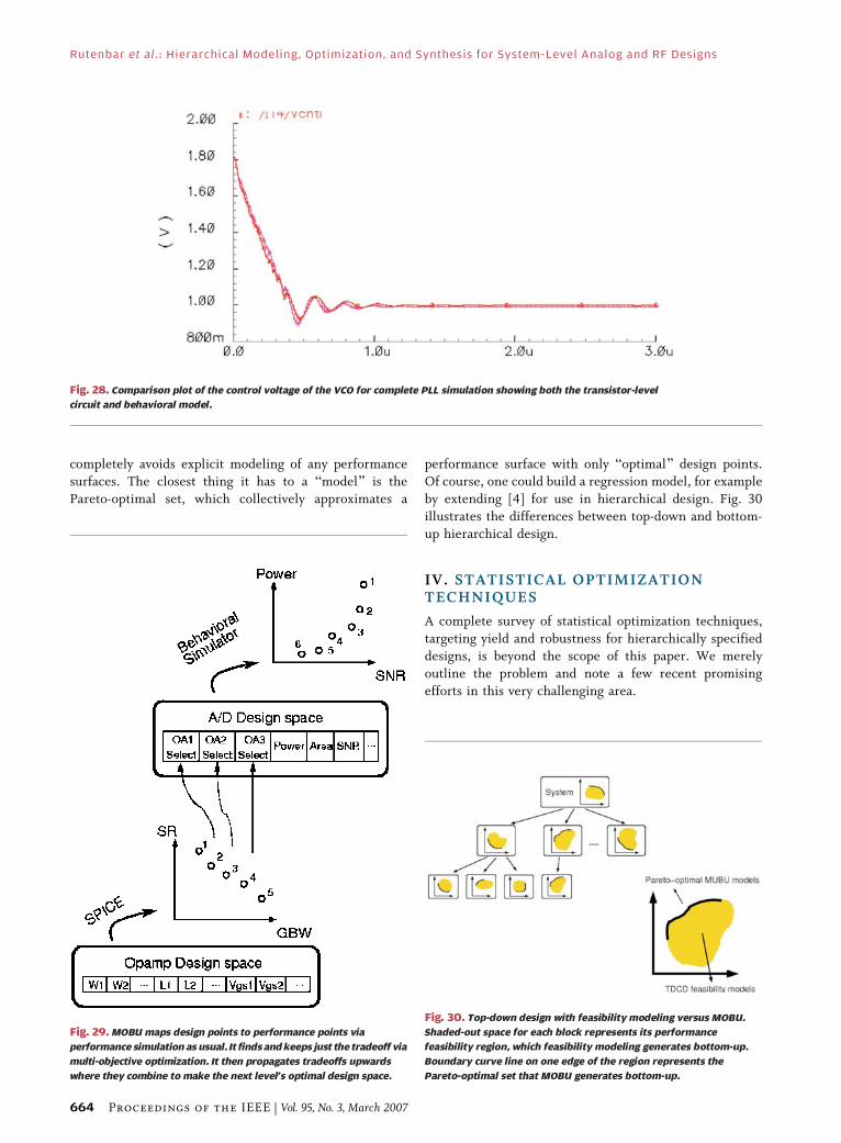
completely avoids explicit modeling of any performance
surfaces. The closest thing it has to a Bmodel[ is the
Pareto-optimal set, which collectively approximates a
performance surface with only Boptimal[ design points.
Of course, one could build a regression model, for example
by extending [4] for use in hierarchical design. Fig. 30
illustrates the differences between top-down and bottom-
up hierarchical design.
IV. STATISTICAL OPTIMIZATIONTECHNIQUES
A complete survey of statistical optimization techniques,
targeting yield and robustness for hierarchically specified
designs, is beyond the scope of this paper. We merely
outline the problem and note a few recent promising
efforts in this very challenging area.
Fig. 28. Comparison plot of the control voltage of the VCO for complete PLL simulation showing both the transistor-level
circuit and behavioral model.
Fig. 29. MOBU maps design points to performance points via
performance simulation as usual. It finds and keeps just the tradeoff via
multi-objective optimization. It then propagates tradeoffs upwards
where they combine to make the next level’s optimal design space.
Fig. 30. Top-down design with feasibility modeling versus MOBU.
Shaded-out space for each block represents its performance
feasibility region, which feasibility modeling generates bottom-up.
Boundary curve line on one edge of the region represents the
Pareto-optimal set that MOBU generates bottom-up.
Rutenbar et al.: Hierarchical Modeling, Optimization, and Synthesis for System-Level Analog and RF Designs
664 Proceedings of the IEEE | Vol. 95, No. 3, March 2007

Industrial design practice not only calls for fully op-
timized nominal design solutions but also expects high
robustness and yield in the light of varying operating con-ditions (supply voltage or temperature variations) and
statistical manufacturing tolerances and mismatches [15],
[16]. Due to these fluctuations, the device parameters and
consequently also the circuit performance characteristics
will show fluctuations. The corresponding parametric yield
is the ratio of the number of acceptable (i.e., functional
and meeting all specifications) to all fabricated IC samples.
The yield of course depends on the nominal design pointchosen for the circuit. Unfortunately, the relation between
the (fluctuating) device parameters and the circuit
performances is in general a nonlinear transformation
that is not known explicitly but has to be simulated. All this
makes yield estimation a time-consuming task, which in
practice is often obtained by Monte Carlo simulations. An
overview of more efficient techniques that trade off
accuracy versus CPU time can be found in [2]. Note thatin practice not only the yield, but in general the robustness
of the design against variations of both technological and
environmental parameters, has to be maximized. This
implies techniques for variability minimization and design
centering.
The most straightforwardVand, sadly, still the most
practically encountered solutionVis to evaluate the circuit
performance not only in the nominal design point, but alsoin a set of predefined worst case process, voltage, and
temperature (P,V,T) corners. The circuit then needs to
satisfy the specifications in all corners. The problem with
this approach is that the CPU time increases with the
number of corners that needs to be simulated and that the
number of corners becomes intractably large in nanometer
technologies. In addition, for any reasonably complex system
level design, we do know not in advance which of these
intractable number of design corners is actually the worstcorner for each individual circuit specification. Corner-based
design also easily leads to overly pessimistic worst case
design. Hence, the current trend is to move towards true
statistical yield optimization, where the statistical distribu-
tion of the parameter variations is considered.
Handling difficult statistics, with complex correlations,
for complex circuits with difficult-to-simulate analog
behaviors, remains a challenge. We simply mention afew notable efforts here. In the area of simulation-based
synthesis, the WiCked approach [17] uses worst case
parameter distances as robustness objectives to obtain a
nominal design that satisfies all specifications with as
much safety margin as possible for process variations. The
resulting formulation is the same as for design centering
and can be solved efficiently using the generalized
boundary curve. Design centering, however, still remainsa second step after the nominal design. The efficient
projection-based quadratic modeling ideas of the ROAD
approach [91] actually apply very effectively to the
statistical case, since one can build statistical response
surfaces with this idea. In combination with efficient
numerical techniques like APEX [103] to estimate the pdfs
of nonlinear circuits, ROAD can be used as an effective
post-nominal robust optimizer. An example appears inFig. 31, which shows a successful post-nominal robustness
optimization for an RF LNA. Finally, the convex modeling
ideas mentioned in Section III-B can also be applied in this
context, e.g., [104] formulates a novel system-level
exploration methodology based on geometric centering
ideas that can be rendered in a convex form.
Fig. 31. Applying ROAD methodology for post-nominal statistical robustness optimization on RF LNA in 0.25-�m SiGe process [91].
Rutenbar et al. : Hierarchical Modeling, Optimization, and Synthesis for System-Level Analog and RF Designs
Vol. 95, No. 3, March 2007 | Proceedings of the IEEE 665

V. CONCLUSION
In this paper, we have attempted to review the recent state
of the art in hierarchical analog synthesis, with a strongemphasis on associated techniques for computer-aided
model generation and optimization. There are industrially
useful and commercially available tools at the cell
levelVtools for analog components with 10–100 devices.
However, successful component-level tools do not scale
trivially to system-level applications. These hierarchically
specified designs need to optimize many competing
continuous-valued performance specifications, which de-pend on the circuit designer’s abilities to successfully exploit
a range of nonlinear behaviors across levels of abstraction
from devices to circuits to systems. For purposes of synthesis
or verification, these designs are not tractable when
considered Bflat.[ These designs must be approached with
hierarchical tools that deal with the system’s intrinsic design
hierarchy. We reviewed recent ideas in analog modeling and
synthesis that specifically deal with the hierarchical natureof practical mixed-signal and RF systems: algorithmic
techniques for automatically extracting a suitable nonlinear
macromodel from a device-level circuit; parametric model-
ing techniques; ideas for hierarchical synthesis, in partic-
ular, numerical techniques for handling the large number of
degrees of freedom in these designs, and for exploring the
space of performance tradeoffs early in the design process.Finally, we briefly touched on emerging ideas for accom-
modating models of statistical manufacturing variations in
these tools and flows.
As more analog and RF designs migrate onto difficult
SOC-style digital platforms, we expect to see a continuing
demand for these sorts of hierarchically oriented modeling
and synthesis tools and, in particular, tools to help designs
deal with the challenges to circuit robustness posed bynanometer technologies. h
Acknowledgment
The authors would like to thank A. Singhee of Carnegie
Mellon University, Pittsburgh, PA, who provided valuable
comments and proofreading at various early stages of the
development of this manuscript and detailed material on
Pareto-optimal fronts used in Section III. J. Roychowdhury
would like to thank N. Dong (TI), X. Lai (University ofMinnesota), and T. Mei (University of Minnesota), on
whose research much of the material here on macro-
modelling and simulation relies. G. Gielen would like to
thank Ph.D. students T. Eeckelaert, E. Martens, and
T. McConaghy, who have contributed largely to the work
on hierarchical synthesis and performance modeling.
REF ERENCE S
[1] International Technology Roadmap forSemiconductors 2003. [Online]. Available:http://www.public.itrs.net.
[2] G. Gielen and R. Rutenbar, BComputer-aideddesign of analog and mixed-signal integratedcircuits,[ Proc. IEEE, vol. 88, no. 12,pp. 1825–1854, Dec. 2000.
[3] R. A. Rutenbar, G. G. E. Gielen, andB. Antao, Eds., Computer-Aided Designof Analog Integrated Circuits andSystems. Hoboken, NJ: Wiley-IEEE,Apr. 2002.
[4] B. De Smedt and G. Gielen, BWATSON:Design space boundary exploration andmodel generation for analog and RF ICdesign,[ IEEE Trans. Computer-Aided Design,vol. 22, no. 2, pp. 213–224, Feb. 2003.
[5] G. Stehr, H. Graeb, and K. Antreich,BPerformance trade-off analysis of analogcircuits by normal-boundary intersection,’’in Proc. IEEE/ACM Design Automation Conf.(DAC), 2003, pp. 958–963.
[6] R. Harjani, R. Rutenbar, and L. R. Carley,BOASYS: A framework for analog circuitsynthesis,[ IEEE Trans. Computer-AidedDesign, vol. 8, no. 12, pp. 1247–1265,Dec. 1989.
[7] G. Gielen, T. McConaghy, and T. Eeckelaert,BPerformance space modeling forhierarchical synthesis of analog integratedcircuits,[ in Proc. IEEE Design AutomationConf. (DAC), Jun. 2005, pp. 881–886.
[8] B. De Smedt and G. Gielen, BModels forsystematic design and verification offrequency synthesizers,[ IEEE Trans. CircuitsSystems, Part II: Analog Digital SignalProcessing, vol. 46, no. 10, pp. 1301–1308,Oct. 1999.
[9] W. Daems, G. Gielen, and W. Sansen,BSimulation-based generation of posynomial
performance models for the sizing ofanalog integrated circuits,[ IEEE Trans.Computer-Aided Design, vol. 22, no. 5,pp. 517–534, May 2003.
[10] T. Kiely and G. Gielen, BPerformancemodeling of analog integrated circuits usingleast-squares support vector machines,[ inProc. Design, Automation Test Eur. (DATE)Conf., Feb. 2004, pp. 448–453.
[11] H. Liu, A. Singhee, R. Rutenbar, andL. R. Carley, BRemembrance of circuits past:Macromodeling by data mining in largeanalog design spaces,[ in Proc. IEEE/ACMDesign Automation Conf. (DAC), Jun. 2002,pp. 437–442.
[12] T. McConaghy, T. Eeckelaert, and G. Gielen,BCAFFEINE: Template-free symbolic modelgeneration of analog circuits via canonicalform functions and genetic programming,[in Proc. Design, Automation Test Eur. Conf.(DATE), Mar. 2005, vol. 2, pp. 1082–1087.
[13] T. McConaghy and G. Gielen, BAnalysis ofsimulation-driven numerical performancemodeling techniques for application toanalog circuit optimization,[ in Proc. IEEEInt. Symp. Circuits Systems (ISCAS),May 2005, vol. 2, pp. 1298–1301.
[14] T. McConaghy, T. Eeckelaert, and G. Gielen,BFast-acting CAFFEINE for template-freesymbolic model generation of analog circuitsvia implicit canonical form functions andexplicit introns,[ in Proc. Design, AutomationTest Eur. Conf. (DATE), Mar. 2006.
[15] S. Director, W. Maly, and A. Strojwas,VLSI Design for Manufacturing: YieldEnhancement. Boston, MA: Kluwer, 1990.
[16] J. Zhang and M. Styblinski, Yield andVariability Optimization of IntegratedCircuits. Boston, MA: Kluwer, 1995.
[17] K. Antreich, H. Graeb, and C. Wieser,BCircuit analysis and optimization driven
by worst-case distances,[ IEEE Trans.Computer-Aided Design, vol. 13, no. 1,pp. 57–71, Jan. 1994.
[18] X. Huang, C. S. Gathercole, andH. A. Mantooth, BModeling nonlineardynamics in analog circuits via rootlocalization,[ IEEE Trans. Computer-AidedDesign, vol. 22, no. 7, pp. 895–907, Jul. 2003.
[19] K. Francken, M. Vogels, E. Martens, andG. Gielen, BA behavioral simulation toolfor continuous-time/spl Delta//spl Sigma/modulators,[ in Proc. ICCAD, Nov. 2002,pp. 229–233.
[20] S. X.-D. Tan and C. J.-R. Shi, BEfficientDDD-based term generation algorithm foranalog circuit behavioral modeling,[ in Proc.IEEE ASP-DAC, Jan. 2003, pp. 789–794.
[21] VV, BEfficient DDD-based term generationalgorithm for analog circuit behavioralmodeling,[ in Proc. IEEE DATE Conf.,Mar. 2003, pp. 1009–1108.
[22] VV, BEfficient very large scale integrationpower/ground network sizing based onequivalent circuit modeling,[ IEEE Trans.Computer-Aided Design, vol. 22, no. 3,pp. 277–284, Mar. 2003.
[23] Y. Qicheng and C. Sechen, BA unifiedapproach to the approximate symbolicanalysis of large analog integrated circuits,[IEEE Trans. Cts. Syst.VI: Fund. Th. Appl.,pp. 656–669, Aug. 1996.
[24] W. Daems, G. Gielen, and W. Sansen,BA fitting approach to generate symbolicexpressions for linear and nonlinear analogcircuit performance characteristics,[ in Proc.IEEE DATE Conf., Mar. 2002, pp. 268–273.
[25] P. Vanassche, G. Gielen, and W. Sansen,BConstructing symbolic models for theinput/output behavior of periodicallytime-varying systems using harmonic
Rutenbar et al.: Hierarchical Modeling, Optimization, and Synthesis for System-Level Analog and RF Designs
666 Proceedings of the IEEE | Vol. 95, No. 3, March 2007

transfer matrices,[ in Proc. IEEE DATE Conf.,Mar. 2002, pp. 279–284.
[26] L. Hongzhou, A. Singhee, R. Rutenbar, andL. R. Carley, BRemembrance of circuits past:Macromodeling by data mining in largeanalog design spaces,[ in Proc. IEEE DAC,Jun. 2002, pp. 437–442.
[27] D. Schreurs, J. Wood, N. Tufillaro,D. Usikov, L. Barford, and D. E. Root,BThe construction and evaluation ofbehavioral models for microwave devicesbased on time-domain large-signalmeasurements,[ in Proc. IEEE IEDM,Dec. 2000, pp. 819–822.
[28] J. Wood and D. E. Root, BThe behavioralmodeling of microwave/RF ICs usingnon-linear time series analysis,[ in IEEEMTT-S Dig., Jun. 2003, pp. 791–794.
[29] L. A. Zadeh and C. A. Desoer, Linear SystemTheory: The State-Space Approach, ser.System Science. New York: McGraw-Hill,1963.
[30] L. T. Pillage and R. A. Rohrer, BAsymptoticwaveform evaluation for timing analysis,[IEEE Trans. Computer-Aided Design, vol. 9,pp. 352–366, Apr. 1990.
[31] E. Chiprout and M. S. Nakhla, AsymptoticWaveform Evaluation. Norwell, MA:Kluwer, 1994.
[32] K. Gallivan, E. Grimme, and P. Van Dooren,BAsymptotic waveform evaluation via aLanczos method,[ Appl. Math. Lett., vol. 7,pp. 75–80, 1994.
[33] P. Feldmann and R. W. Freund, BEfficientlinear circuit analysis by Pade approximationvia the Lanczos process,[ IEEE Trans.Computer-Aided Design, vol. 14, no. 5,pp. 639–649, May 1995.
[34] R. W. Freund and P. Feldmann, BEfficientsmall-signal circuit analysis and sensitivitycomputations with the Pvl algorithm,[ inProc. ICCAD, Nov. 1995, pp. 404–411.
[35] Y. Saad, Iterative Methods for Sparse LinearSystems. Boston, MA: PWS, 1996.
[36] E. J. Grimme, BKrylov projection methodsfor model reduction,[ Ph.D. dissertation,EE Dep., Univ. Illinois, Urbana-Champaign,1997.
[37] L. M. Silveira, M. Kamon, I. Elfadel, andJ. White, BA coordinate-transformed Arnoldialgorithm for generating guaranteed stablereduced-order models of RLC circuits,[ inProc. ICCAD, Nov. 1996, pp. 288–294.
[38] K. J. Kerns, I. L. Wemple, and A. T. Yang,BStable and efficient reduction of substratemodel networks using congruencetransforms,[ in Proc. ICCAD, Nov. 1995,pp. 207–214.
[39] R. Freund and P. Feldmann, BReduced-ordermodeling of large passive linear circuits bymeans of the SyPVL algorithm,[ in Proc.ICCAD, Nov. 1996, pp. 280–287.
[40] Odabasioglu, M. Celik, and L. T. Pileggi,BPRIMA: Passive reduced-orderinterconnect macromodelling algorithm,[in Proc. ICCAD, Nov. 1997, pp. 58–65.
[41] VV, BPRIMA: Passive reduced-orderinterconnect macromodelling algorithm,[IEEE Trans. Computer-Aided Design,pp. 645–654, Aug. 1998.
[42] Z. Bai, R. Freund, and P. Feldmann, BHow tomake theoretically passive reduced-ordermodels passive in practice,[ in Proc. IEEECICC, May 1998, pp. 207–210.
[43] R. Freund, BPassive reduced-order modelsfor interconnect simulation and theircomputation via Krylov-subspacealgorithms,[ in Proc. IEEE DAC, Jun. 1999,pp. 195–200.
[44] J.-R. Li and J. White, BEfficient modelreduction of interconnect via approximatesystem gramians,[ in Proc. ICCAD,Nov. 1999, pp. 380–383.
[45] J. Phillips, L. Daniel, and L. M. Silveira,BGuaranteed passive balancingtransformations for model order reduction,[in Proc. IEEE DAC, Jun. 2002, pp. 52–57.
[46] M. Kamon, F. Wang, and J. White,BGenerating nearly optimally compactmodels from Krylov-subspace basedreduced-order models,[ IEEE Trans. Cts.Syst.VII: Sig. Proc., pp. 239–248, Apr. 2000.
[47] J. Roychowdhury, BMPDE methods forefficient analysis of wireless systems,[in Proc. IEEE CICC, May 1998.
[48] VV, BReduced-order modelling of lineartime-varying systems,[ in Proc. ICCAD,Nov. 1998.
[49] VV, BReduced-order modelling oftime-varying systems,[ IEEE Trans. Cts.Syst.VII: Sig. Proc., vol. 46, no. 10,Nov. 1999.
[50] VV, BAnalysing circuits withwidely-separated time scales using numericalPDE methods,[ IEEE Trans. Cts. Syst.VI:Fund. Th. Appl., May 2001.
[51] K. S. Kundert, J. K. White, andA. Sangiovanni-Vincentelli, Steady-StateMethods for Simulating Analog and MicrowaveCircuits. Boston, MA: Kluwer, 1990.
[52] M. Rosch and K. J. Antreich, BSchnellstationare simulation nichtlinearerschaltungen im frequenzbereich,[ AEU,vol. 46, no. 3, pp. 168–176, 1992.
[53] R. Telichevesky, K. Kundert, and J. White,BEfficient steady-state analysis based onmatrix-free Krylov subspace methods,[ inProc. IEEE DAC, 1995, pp. 480–484.
[54] J. Phillips, BModel reduction of time-varyinglinear systems using approximate multipointKrylov-subspace projectors,[ in Proc. ICCAD,Nov. 1998.
[55] M. Schetzen, The Volterra and WienerTheories of Nonlinear Systems. New York:Wiley, 1980.
[56] Nayfeh and B. Balachandran, AppliedNonlinear Dynamics. New York: Wiley,1995.
[57] J. Phillips, BProjection frameworks for modelreduction of weakly nonlinear systems,[in Proc. IEEE DAC, Jun. 2000.
[58] VV, BProjection-based approaches formodel reduction of weakly nonlinear,time-varying systems,[ IEEE Trans.Computer-Aided Design, vol. 22, no. 2,pp. 171–187, Feb. 2000.
[59] W. Rugh, Nonlinear System TheoryVTheVolterra-Wiener Approach. Baltimore, MD:Johns Hopkins Univ. Press, 1981.
[60] P. Li and L. Pileggi, BNORM: Compactmodel order reduction of weakly nonlinearsystems,[ in Proc. IEEE DAC, Jun. 2003,pp. 472–477.
[61] J. Katzenelson and L. H. Seitelman, BAniterative method for solution of nonlinearresistive networks,[ AT&T Bell Laboratories,Tech. Rep. TM65-1375-3.
[62] F. Ohtsuki and Kumagai, BExistencetheorems and a solution algorithm forpiecewise linear resistor networks,[ SIAM J.Math. Anal., vol. 8, Feb. 1977.
[63] M. Rewienski and J. White, BA trajectorypiecewise-linear approach to model orderreduction and fast simulation of nonlinearcircuits and micromachined devices,[in Proc. ICCAD, Nov. 2001.
[64] N. Dong and J. Roychowdhury, BPiecewisepolynomial model order reduction,[ in Proc.IEEE DAC, Jun. 2003, pp. 484–489.
[65] L. W. Nagel, BSPICE2: A computer programto simulate semiconductor circuits,[ Ph.D.dissertation, EECS Dep., Univ. Calif.Berkeley, Elec. Res. Lab., 1975,Memo. ERL-M520.
[66] T. L. Quarles, BAnalysis of performance andconvergence issues for circuit simulation,[Ph.D. dissertation, EECS Dep., Univ. Calif.Berkeley, Elec. Res. Lab., Apr. 1989,Memo. UCB/ERL M89/42.
[67] M. Schwab, BDetermination of the steadystate of an oscillator by a combinedtime-frequency method,[ IEEE Trans.Microwave Theory Tech., vol. 39,pp. 1391–1402, Aug. 1991.
[68] O. Narayan and J. Roychowdhury,BAnalysing oscillators using multitimePDEs,[ IEEE Trans. Cts. Syst.VI: Fund. Th.Appl., vol. 50, no. 7, pp. 894–903, Jul. 2003.
[69] E. Ngoya and R. Larcheveque, BEnveloptransient analysis: A new method for thetransient and steady state analysis ofmicrowave communication circuits andsystems,[ in Proc. IEEE MTT Symp., 1996.
[70] W. Gardner, Introduction to RandomProcesses. New York: McGraw-Hill, 1986.
[71] Hajimiri and T. H. Lee, BA general theory ofphase noise in electrical oscillators,[ IEEE J.Solid-State Cts., vol. 33, pp. 179–194,Feb. 1998.
[72] Demir, E. Liu, A. L. Sangiovanni-Vincentelli,and I. Vassiliou, BBehavioral simulationtechniques for phase/delay-locked systems,[in Proc. Custom Integrated Circuits Conf.,May 1994, pp. 453–456.
[73] Costantini, C. Florian, and G. Vannini,BVCO behavioral modeling based on thenonlinear integral approach,[ in IEEE Int.Symp. Circuits and Syst., May 2002,vol. 2, pp. 137–140.
[74] L. Wu, H. W. Jin, and W. C. Black,BNonlinear behavioral modeling andsimulation of phase-locked and delay-lockedsystems,[ in Proc. IEEE CICC, May 2000,pp. 447–450.
[75] M. F. Mar, BAn event-driven pll behavioralmodel with applications to design drivennoise modeling,[ in Proc. Behav. Model Simul.(BMAS), 1999.
[76] P. Vanassche, G. G. E. Gielen, andW. Sansen, BBehavioral modeling ofcoupled harmonic oscillators,[ IEEE Trans.Computer-Aided Design Integrated CircuitsSyst., vol. 22, no. 8, pp. 1017–1026,Aug. 2003.
[77] K. Kundert. (2002). Predicting the phasenoise and jitter of PLL-based frequencysynthesizers. [Online]. Available:www.designers-guide.com.
[78] Demir, A. Mehrotra, and J. Roychowdhury,BPhase noise in oscillators: A unifyingtheory and numerical methods forcharacterization,[ IEEE Trans. Cts. Syst.VI:Fund. Th. Appl., vol. 47, pp. 655–674,May 2000.
[79] Demir and J. Roychowdhury, BA reliableand efficient procedure for oscillatorPPV computation, with phase noisemacromodelling applications,[ IEEE Trans.Cts. Syst.VI: Fund. Th. Appl., pp. 188–197,Feb. 2003.
[80] J. L. Stensby, Phase-Locked Loops: Theory andApplications. Boca Raton, FL: CRC, 1997.
[81] N. Dong and J. Roychowdhury, BAutomatedextraction of broadly-applicable nonlinear
Rutenbar et al. : Hierarchical Modeling, Optimization, and Synthesis for System-Level Analog and RF Designs
Vol. 95, No. 3, March 2007 | Proceedings of the IEEE 667

analog macromodels from SPICE-leveldescriptions,[ in Proc. IEEE CICC, Oct. 2004.
[82] X. Lai and J. Roychowdhury, BCapturinginjection locking via nonlinear phase domainmacromodels,[ IEEE MTT, vol. 52, no. 9,pp. 2251–2261, Sep. 2004.
[83] VV, BFast, accurate prediction of PLL jitterinduced by power grid noise,[ in Proc. IEEECustom Integrated Circuits Conf., May 2004.
[84] X. Lai, Y. Wan, and J. Roychowdhury, BFastPLL simulation using nonlinear VCOmacromodels for accurate prediction of jitterand cycle-slipping due to loop non-idealitiesand supply noise,[ in Proc ASP-DAC,Jan. 2005.
[85] S. K. Tiwary and R. A. Rutenbar, BScalabletrajectory methods for on-demand analogmacromodel extraction,[ in Proc. ACM/IEEEDesign Automation Conf., Jun. 2005.
[86] S. K. Tiwary, BScalable trajectory methodsfor on-demand analog macromodelextraction,[ Ph.D. dissertation, Dep.Electrical Computer Eng., Carnegie MellonUniv., Pittsburgh, PA, May 2006.
[87] M. Krasnicki, R. Phelps, R. A. Rutenbar, andL. R. Carley, BMAELSTROM: Efficientsimulation-based synthesis for custom analogcells,[ in Proc. DAC, 1999, pp. 945–950.
[88] R. Phelps, M. Krasnicki, R. A. Rutenbar,L. R. Carley, and J. R. Hellums, BA case studyof synthesis for industrial-scale analog IP:Redesign of the equalizer/filter frontend foran ADSL CODEC,[ in Proc ACM/IEEE DAC,Jun. 2000, pp. 1–6.
[89] G. Van der Plas, G. Debyser, F. Leyn,K. Lampaert, J. Vandenbussche, G. Gielen,W. Sansen, P. Veselinovic, and D. Leenaerts,BAMGIE: A synthesis environment forCMOS analog integrated circuits,[IEEE Trans. Computer-Aided Design, vol. 20,no. 9, pp. 1037–1058, Sep. 2001.
[90] K. Antreich, J. Eckmller, H. Grb, M. Pronath,F. Schenkel, R. Schwencker, and S. Zizala,BWicked: Analog circuit synthesisincorporating mismatch,[ in IEEE CustomIntegrated Circuits Conf. (CICC), May 2000.
[91] X. Li and L. Pileggi, BRobust analog/RFcircuit design with projection-basedposynomial,[ in Proc. Int. Conf.Computer-Aided Design, Nov. 2004.
[92] X. Li, J. Le, L. Pileggi, and A. J. Strojwas,BProjection-based performance modeling forinter/intra-die variations,[ in Proc. Int. Conf.Computer-Aided Design, Nov. 2005.
[93] Y. Freund, BBoosting a weak learningalgorithm by majority,[ InformationComputation, vol. 121, no. 2, pp. 256–285,1995.
[94] F. De Bernardinis, M. I. Jordan, andA. Sangiovanni Vincentelli, BSupport vectormachines for analog circuit performancerepresentation,[ in Proc. ACM/IEEE DAC,Jun. 2003.
[95] S. K. Tiwary, S. Velu, R. A. Rutenbar, andT. Mukherjee, BPareto optimal modeling forefficient PLL optimization,[ in Proc. Int.Conf. Modeling Simulation in Microsystems,Mar. 2004.
[96] I. Das and J. E. Dennis, BNormal-boundaryintersection: A new method for generatingthe pareto surface in nonlinear multicriteriaoptimization problems,[ SIAM J. Optim.,vol. 8, no. 3, pp. 631–657, Aug. 1998.
[97] A. Singhee, BPerformance feasibility regionsof analog circuits: Computation andapplication,[ Dep. Electrical and ComputerEng., Carnegie Mellon Univ., Pittsburgh, PA,May 2005, Ph.D. Qualifying Exam Paper.
[98] M. Hershenson, S. Boyd, and T. H. Lee,BGPCAD: A tool for CMOS opampsynthesis,[ in Proc. IEEE/ACM Int. Conf.Computer-Aided Design, San Jose, CA, 1998,pp. 296–303.
[99] M. Hershenson, A. Hajimiri, S. S. Mohan,S. P. Boyd, and T. H. Lee, BDesign andoptimization of LC oscillators,[ in Proc. IEEE/ACM Int. Conf. Computer Aided Design,San Jose, CA, Nov. 1999.
[100] M. Hershenson, BDesign of pipelineanalog-to-digital converters via geometricprogramming,[ in Proc. ACM/IEEE ICCAD,Nov. 2002.
[101] D. M. Colleran et al., BOptimization ofphase-locked loop circuits via geometricprogramming,[ in Proc. IEEE CICC,May 2003.
[102] T. K. Ogawa and K. Kundert, BVCO jittersimulation and its comparison withmeasurement,[ in Proc. ASP-DAC, Jan. 1999.
[103] X. Li and L. Pileggi, BAsymptotic probabilityextraction for non-normal distributions ofcircuit performance,[ in Proc. Int. Conf.Computer-Aided Design, Nov. 2004.
[104] X. Li, J. Wang, W. Chiang, and L. Pileggi,BPerformance-centering optimization forsystem-level analog design exploration,[in Proc. Int. Conf. Computer-Aided Design,Nov. 2005.
[105] H. Chang et al., BA top-down, constraint-driven design methodology for analogintegrated circuits,[ in Proc. IEEE CustomIntegrated Circuits Conf. (CICC), 1992,pp. 8.4.1–8.4.6.
[106] H. Chang, E. Charbon, U. Choudhury,A. Demir, E. Felt, E. Liu, E. Malavasi,A. Sangiovanni-Vincentelli, and I. Vassiliou,A Top-Down, Constraint-Driven DesignMethodology for Analog IntegratedCircuits. Boston, MA: Kluwer, 1997.
ABOUT TH E AUTHORS
Rob A. Rutenbar (Fellow, IEEE) received the Ph.D. degree in
computer engineering from the University of Michigan, Ann
Arbor, in 1984.
He subsequently joined the faculty at Carnegie Mellon
University (CMU), Pittsburgh, PA, where he is currently the
Stephen J. Jatras Professor of Electrical and Computer Engineer-
ing. His research focuses on optimization-based methods for
custom circuit synthesis and modeling, for statistical analysis of
deeply scaled circuits, and for automatic layout of complex
analog and digital designs. He has published over 100 papers in
the field of CAD for circuits and systems In 1998, on a leave of absence from CMU, he
cofounded Neolinear, Inc., and served as its Chief Scientist until its acquisition by
Cadence in 2004. He chaired Cadence Design Systems’ Analog Technical Advisory Board
from 1992 to 1996.
Dr. Rutenbar is the founding Director of the MARCO/DARPA Focus Center for Circuit
& System Solutions (called FC2S2_), a consortium of 17 major U.S. universities, supporting
roughly 50 faculty investigators, funded by the U.S. semiconductor community and U.S.
DOD (DARPA) to address future circuit design challenges. He is a 2001 winner of the
Semiconductor Research Corporation (SRC) Aristotle Award for excellence in education.
In 2002 he was honored with a University of Michigan Alumni Society Merit Award for
Electrical Engineering. He is also a 2004 winner of an SRC Technical Excellence Award
for his contributions to BElectronic Design Automation for Analog/Mixed-Signal Design[
and recipient of numerous Best Paper awards (e.g., ACM/IEEE Design Automation
Conference, in 1987 and again in 2002). He was the General Chair of the 1996 ACM/IEEE
International Conference on CAD. He is a member of the ACM and Eta Kappa Nu.
Rutenbar et al.: Hierarchical Modeling, Optimization, and Synthesis for System-Level Analog and RF Designs
668 Proceedings of the IEEE | Vol. 95, No. 3, March 2007

Georges G. E. Gielen (Fellow, IEEE) received the
M.Sc. and Ph.D. degrees in electrical engineering
from the Katholieke Universiteit Leuven, Belgium,
in 1986 and 1990, respectively.
In 1990, he was appointed as a Postdoctoral
Research Assistant and Visiting Lecturer at the
Department of Electrical Engineering and Com-
puter Science of the University of California,
Berkeley. From 1991 to 1993, he was a Postdoc-
toral Research Assistant of the Belgian National
Fund of Scientific Research at the ESAT Laboratory of the Katholieke
Universiteit Leuven. In 1993, he was appointed Assistant Professor at the
Katholieke Universiteit Leuven, where he was promoted to full Professor
in 2000. His research interests are in the design of analog and mixed-
signal integrated circuits, especially in analog and mixed-signal CAD tools
and design automation (modeling, simulation and symbolic analysis,
analog synthesis, analog layout generation, analog and mixed-signal
testing). He is a coordinator or partner of several (industrial) research
projects in this area. He has authored or coauthored two books and more
than 300 papers in edited books, international journals, and conference
proceedings.
Dr. Gielen serves regularly as a member of the program committees of
international conferences (DAC, ICCAD, ISCAS, DATE, CICC), and served as
General Chair of the DATE conference in 2006. He has been a member of
editorial boards of international journals including IEEE TRANSACTIONS ON
CIRCUITS AND SYSTEMS, Springer International Journal on Analog Integrated
Circuits and Signal Processing, and Elsevier Integration. He received the
1995 Best Paper Award in the John Wiley International Journal on Circuit
Theory and Applications, and was the 1997 Laureate of the Belgian Royal
Academy on Sciences, Literature and Arts in the discipline of Engineering.
He received the 2000 Alcatel Award from the Belgian National Fund of
Scientific Research for his innovative research in telecommunications
and won the DATE 2004 Best Paper Award. He served as and elected
member of the Board of Governors of the IEEE Circuits And Systems (CAS)
society and as Chairman of the IEEE Benelux CAS chapter. He served as
the President of the IEEE Circuits And Systems (CAS) Society in 2005.
Jaijeet Roychowdhury (Senior Member, IEEE)
received the B.S. degree in electrical engineering
from the Indian Institute of Technology, Kanpur, in
1987, and the Ph.D degree in electrical engineering
and computer science from the University of
California, Berkeley, in 1993.
From 1993 to 1995, he was with the CAD Lab of
AT&T’s Bell Laboratories, Allentown, PA. From
1995 to 2000, he was with the Communication
Sciences Research Division of Lucent’s Bell Labo-
ratories, Murray Hill, NJ, and from 2000 to 2001, with CeLight, Inc., an
optical networking startup, Silver Spring, MD. In 2001, he joined the ECE
Department and the Digital Technology Center of the University of
Minnesota, Minneapolis, as an Associate Professor. His professional
interests include the design, analysis, and simulation of electronic,
electro-optical and mixed-domain systems, particularly for high-speed
and high-frequency communications. He holds ten patents.
Dr. Roychowdhury has received Distinguished or Best Paper Awards
at ICCAD 1991, DAC 1997, ASP-DAC 1997 and ASP-DAC 1999, was cited for
Extraordinary Achievement by Bell Laboratories, and has served on the
Technical Program Committees of DAC, ICCAD, BMAS and SCEE.
Rutenbar et al. : Hierarchical Modeling, Optimization, and Synthesis for System-Level Analog and RF Designs
Vol. 95, No. 3, March 2007 | Proceedings of the IEEE 669


