
1
NOT FOR PUBLICATION WITHOUT APPROVAL OF COMMITTEE ON OPINIONS
SUPERIOR COURT OF NEW JERSEY LAW DIVISION: MERCER COUNTY
Civil Action (Mount Laurel)
OPINION ON FAIR SHARE
METHODOLOGY TO IMPLEMENT THE MOUNT LAUREL AFFORDABLE
HOUSING DOCTRINE FOR THE THIRD ROUND
DOCKET NUMBERS:
MER-L-1550-15
MER-L-1561-15
In the Matter of the Application of the Municipality of Princeton _______________________________ In the Matter of West Windsor Township
Attorneys for Plaintiffs and League of Municipalities: Jeffrey R. Surenian, Esq. Jeffrey R. Surenian and Associates, LLC 707 Union Avenue Suite 301 Brielle, New Jersey 08730 Edward J. Buzak, Esq. THE BUZAK LAW GROUP, LLC Montville Office Park 150 River Road, Suite N-4 Montville, New Jersey 07045 Special Methodology Master: Richard B. Reading 759 State Road Princeton, New Jersey 08540
Attorneys for Fair Share Housing Center: Kevin D. Walsh, Esq. Adam Gordon, Esq. 510 Park Blvd Cherry Hill, New Jersey 08002 Attorney for New Jersey Builders Association: Richard Hoff, Esq. BISGAIER HOFF, LLC 25 Chestnut Street, Suite 3 Haddonfield, New Jersey 08033 Lead Counsel for Developer/Intervenor Group: Thomas F. Carroll, III, Esq. Stephen M. Eisdorfer, Esq. HILL WALLACK LLP 21 Roszel Road P.O. Box 5226 Princeton, New Jersey 08543
2
JACOBSON, A.J.S.C. Table of Contents
I. Introduction.............................................. 4
II. Factual and Procedural History............................ 9
A. Parties’ Positions ..................................... 18
B. The Experts ............................................ 21
1. Dr. Peter Angelides – Offered by the Municipalities .. 21
2. Dr. David Kinsey – Offered by FSHC ................... 23
3. Mr. Daniel McCue – Offered by FSHC ................... 25
4. Mr. Art Bernard, P.P. – Offered by NJBA .............. 26
5. Dr. Robert S. Powell, Jr. – Offered by New Jersey League of Municipalities .................................... 27
6. Mr. Jeffrey G. Otteau – Offered by NJBA .............. 29
III. Fair Share Legal Standard................................ 30
IV. Fair Share Methodology................................... 34
A. Prospective Need Phase Methodology ..................... 34
1. Determine Prior Round Obligations .................... 36
2. Calculate Present Need ............................... 37
3. Calculate Regional Prospective Need .................. 40
a. Predict population growth........................... 41
b. Estimate Population Living in Households............ 51
c. Estimate Growth of Total Households................. 54
d. Estimate LMI household growth during the Prospective Need period......................................... 65
i. Income Qualification Data Used in Determining LMI Household Ratio Calculation ....................... 66
e. Reallocation for age distribution of households..... 86
f. Account for older LMI households with significant housing assets (Angelides proposal)................. 87
g. Aggregate Regional Prospective Need................. 90
4. Allocate Prospective Need to municipalities .......... 91
a. Identify and Exclude Qualified Urban Aid Municipalities...................................... 92

3
b. Calculate Responsibility Factor for Each Municipality as a Share of its Region............................ 93
c. Calculate Capacity Factors for Each Municipality as a Share of its Region................................ 100
i. Income Capacity Factor ........................... 100
ii. Land Capacity Factor ............................. 102
d. Average regional shares of “responsibility” and “capacity" factors and allocate gross Prospective Need to each municipality............................... 106
5. Adjust for Secondary Sources of Supply and Demand ... 107
a. Demolitions........................................ 108
b. Residential conversions ........................... 115
c. Filtering.......................................... 121
d. Reallocation of secondary source adjustment........ 129
e. Calculate Prospective Need by Municipality......... 131
V. Gap Present Need/Phase 2................................ 133
A. Gap Present Need Factual and Procedural History ....... 133
B. Gap Present Need Legal Standard ....................... 139
C. Summary of Methodological Approaches .................. 144
1. Dr. Angelides (for the municipalities) .............. 145
a. Guiding Principles................................. 145
b. Methodological Approach............................ 146
2. Dr. Kinsey (for FSHC) ............................... 149
a. Guiding Principles................................. 149
b. Methodological Approach............................ 151
3. Mr. Bernard (for NJSBA) ............................. 152
4. Special Master Reading .............................. 154
D. Gap Present Need Methodology .......................... 157
1. Gap Period LMI Household Growth ..................... 157
2. Dr. Kinsey’s Adjustments ............................ 171
a. Reallocation of Working Age Household Growth....... 171
b. Gap Period Secondary Source Adjustments............ 174
3. Dr. Angelides’ Adjustments .......................... 178
a. LMI households living in affordable housing........ 179
4
b. LMI households with significant housing assets..... 192
c. Overlap with Traditional Present Need.............. 193
VI. Consolidated Affordable Housing Obligations............. 198
A. Calculate and Apply Twenty Percent Cap ................ 200
B. Calculate Municipal Fair Share Affordable Housing Obligations ........................................... 201
VII. Housing Market Analysis................................. 202
VIII. Conclusion............................................. 217
I. Introduction
The present matter has arisen out of declaratory judgment
actions filed with this court by eleven of twelve Mercer County
municipalities seeking to establish Third Round Housing Elements
and Fair Share Plans under New Jersey’s Mount Laurel Affordable
Housing Doctrine. In Re Adoption of N.J.A.C. 5:96 and 5:97 by New
Jersey Council on Affordable Housing, 221 N.J. 1 (2015) (“Mount
Laurel IV”); S. Burlington County NAACP v. Twp. of Mount Laurel,
67 N.J. 151, 174 (1975) (“Mount Laurel I”); In re Adoption of
N.J.A.C. 5:94 & 5:95, 390 N.J. Super. 1, 15 (App. Div. 2007),
certif. denied, 192 N.J. 72 (2007). The declaratory judgment
actions were filed in response to the New Jersey Supreme Court’s
2015 decision that declared the Council on Affordable Housing
(“COAH”) defunct and reinstated the courts as “the forum of first
instance for evaluating municipal compliance with Mount Laurel.”
Mount Laurel IV, 221 N.J. at 20. In 1985, the New Jersey
Legislature adopted the Fair Housing Act (“FHA”), N.J.S.A. 52:27D-
301 to -329, and created COAH to oversee municipal efforts to
5
satisfy their constitutionally mandated affordable housing
obligations. But, having concluded that COAH was “not capable of
functioning as intended by the FHA” when the agency failed to enact
judicially acceptable Third Round rules after being given multiple
extensions of time, the Supreme Court directed trial courts to
both establish affordable housing obligations for New Jersey’s
municipalities and certify municipal plans to meet those
obligations through declaratory judgment actions. Mount Laurel IV,
221 N.J. at 24-29. In the more than two and a half years following
the filing of the Mercer County declaratory judgment actions, three
small municipalities dismissed their complaints, citing the
expense of the litigation; six have entered settlements with Fair
Share Housing Center (“FSHC”) that are moving through the
compliance process, seeking judicial approval of their Housing
Elements and Fair Share Plans; and two—-Princeton and West Windsor—
-remain litigants in the proceedings to establish a fair share
methodology, which is the subject of this decision.
In Mount Laurel IV, 221 N.J. at 3-4, the Supreme Court
reaffirmed its commitment to ensuring that New Jersey’s
municipalities create a “realistic opportunity” for producing
their fair shares of the regional Present and Prospective Need for
low and moderate income (“LMI”) housing. Recognizing COAH’s
failure to address the constitutional obligation administratively,
the Court directed the trial courts to follow “as closely as
6
possible the FHA’s processes,” id. at 6, as implemented by COAH in
determining municipal fair share obligations and reviewing the
municipal zoning ordinances proposed to achieve constitutional
compliance with those obligations. Notably, the Supreme Court
directed the trial courts “not to become a replacement agency for
COAH,” nor to become “an alternate form of statewide administrative
decision maker for unresolved policy details” that remained
following COAH’s inability to adopt regulations governing the
Third Round. Id. at 29. Rather, the trial courts were directed
to utilize previous methodologies developed in the First and Second
Round rules by COAH to “establish present and prospective statewide
and regional affordable housing need.” Id. at 30.
The determination of municipal affordable housing obligations
requires trial courts to once again delve into the technical
complexities involved in developing a methodology to calculate
numerical affordable housing needs, bringing to mind the first
such effort in AMG Realty Co. v. Township of Warren, 207 N.J.
Super. 388 (Law Div. 1984) (Serpentelli, J.S.C) (“AMG”). After
recognizing that the development of a methodology to allocate fair
share obligations to municipalities was the “primary step” in
achieving the ultimate goal of providing more affordable housing
in New Jersey and satisfying the constitutional mandate imposed by
the Mount Laurel doctrine, the AMG court went on to detail the
intricate steps it endorsed in establishing a numerical fair share
7
obligation for Warren Township. Its consideration of population
projection models, employment factors, and computation of median
incomes addressed issues that remain subjects of dispute today,
more than thirty years later, and even after COAH developed its
own methodologies in the First and Second Rounds pursuant to the
FHA, and made three attempts to enact Third Round rules that
complied with the Mount Laurel doctrine. Indeed, the AMG court’s
observation that, “The pivotal question is not whether the numbers
are too high or low, but whether the methodology that produces the
numbers is reasonable,” id. at 453, remains as apt today as it was
in 1984. And the challenge facing this court is the same one
confronting the AMG court: “to make the subject matter easily
intelligible while at the same time not sacrificing accuracy and
thoroughness.” Id. at 450. In assuming this challenge, the court
is cognizant that the endeavor “involves highly controversial
economic, sociological and policy questions of innate difficulty
and complexity.” Oakwood at Madison, Inc. v. Twp. Of Madison, 72
N.J. 481, 533 (1977). In fact, “providing suitable and affordable
housing for citizens of low and moderate incomes” remains “one of
the most difficult constitutional, legal and social issues of our
day.” In re Adoption of N.J.A.C. 5:94 & 5:95 By New Jersey Council
on Affordable Housing, 390 N.J. Super. at 31. If anything, the
passage of time since the establishment of the Mount Laurel
doctrine has done little to lessen the controversy, as COAH’s three
8
attempts to adopt satisfactory Third Round rules and the ensuing
litigation leading to this proceeding demonstrate.
Finally, as the Supreme Court pointed out in S. Burlington
County NAACP v. Twp. of Mount Laurel, 92 N.J. 158 (1983)(“Mount
Laurel II”), and as has been confirmed in this case, fair share
determinations are the most time-consuming and difficult part of
Mount Laurel litigation:
The most troublesome issue in Mount Laurel litigation is the determination of fair share. It takes the most time, produces the greatest variety of opinions, and engenders doubt as to the meaning and wisdom of Mount Laurel. Determination of fair share has required resolution of three separate issues: identifying the relevant region, determining the present and prospective housing needs, and allocating those needs to the municipality or municipalities involved. Each of these issues produces a morass of facts, statistics, projections, theories and opinions sufficient to discourage even the staunchest supporters of Mount Laurel. The problem is capable of monopolizing counsel’s time for years, overwhelming trial courts and inundating reviewing courts with a record on review of superhuman dimensions. [92 N.J. at 248.]
Notably, the Supreme Court also recognized that the “tools for
calculating present and prospective need and its allocation are
imprecise.” Id. at 257. That imprecision did not deter the Court
from directing the trial courts to determine actual numerical
obligations for municipalities to satisfy, “not because we think
scientific accuracy is possible, but because we believe the

9
requirement is most likely to achieve the goals of Mount Laurel.”
Ibid.
The truth of those observations has certainly been borne out
in the present proceeding, which consumed more than forty trial
days and produced a record containing approximately 300 exhibits.
The court reviewed innumerable charts, years of demographic data,
and conflicting statistical analyses. The court also listened
carefully to testimony from six expert witnesses, two of whom
testified for more than twelve days each. Given the importance of
the endeavor, however, the court placed very few limitations on
the presentation of testimony and evidence in order to allow the
parties to compile as complete a record as possible for judicial
review. This decision examines that record and, with acknowledged
imprecision, but a commitment to achieving reasonable results,
adopts a fair share methodology and numerical obligations to guide
Princeton and West Windsor in satisfying their constitutional
responsibility to provide affordable housing.
II. Factual and Procedural History
In Mount Laurel IV, 221 N.J. at 34, the Supreme Court not
only recognized that the administrative process established in the
FHA had become non-functioning, but explicitly directed
municipalities to return to the courts to obtain judgments of
compliance with their constitutional obligations to provide
10
affordable housing, as had been the case prior to adoption of the
FHA and the creation of COAH. Acknowledging that a return to the
courts would involve some disruption from the administrative
process that the towns had followed previously, the Court
established a transition period of ninety days, after which eleven
of the twelve Mercer County municipalities filed declaratory
judgment actions in the summer of 2015 seeking to obtain approval
of their Housing Elements and Fair Share Plans. This court
appointed a special compliance master for each town to review their
proposed Housing Elements and make recommendations to the court as
to whether the municipal Plans passed muster in terms of providing
a realistic opportunity for the creation of LMI housing.
However, since COAH had not adopted Third Round rules to
establish the methodology for determining the numerical fair share
obligation for each town, that task fell to the trial courts. This
court consolidated all of the Mercer County declaratory judgment
actions for the sole purpose of determining that methodology. Each
town would then be treated separately for compliance purposes once
a methodology was established. Knowing that determination of a
methodology to ascertain numerical affordable housing need
presented highly complex and technical issues, the court retained
a Special “Methodology” Master in cooperation with the Mount Laurel
judges in Ocean and Monmouth Counties—-the two other Counties
making up Region 4 under prior COAH practice. That Special Master

11
is economic consultant Richard Reading, who assisted the court
throughout the proceedings by reviewing expert reports, making
recommendations to the court regarding the many aspects of the
methodology where the experts differed, and testifying at the
trial. Mr. Reading provided invaluable assistance to the court in
evaluating the distinctly different methodologies proffered by
both sides to determine municipal fair share obligations. Upon
the court’s completion of its fair share model, the court provided
the results to Mr. Reading for him to calculate the statewide,
regional, and municipal obligations that are set forth in this
decision.
Likely anticipating that the courts would be put in the
position of determining a fair share methodology due to COAH’s
inaction, Fair Share Housing Center, an established affordable
housing advocacy group and a litigant in many affordable housing
cases arising under the Mount Laurel doctrine, produced a report
in April 2015 presenting a methodology to determine LMI housing
obligations in New Jersey for the period 1999-2025, which it
offered as an alternative to COAH’s un-adopted Third Round rules.
In June of 2015, a group of municipalities entered into a shared
services agreement with Rutgers University to produce a fair share
affordable housing methodology and report of their own, but that
report was delayed until December 30, 2015, after Econsult
Solutions, Inc. (“Econsult”), replaced Rutgers University as the
12
towns’ consultant due to the unexpected incapacity of Rutgers
professor, Dr. Robert Burchell, who had been a long-time COAH
consultant and lead analyst under the Rutgers agreement.
Pursuant to the Supreme Court’s Mount Laurel IV directive,
eleven of the twelve Mercer County municipalities filed
declaratory judgment actions in the summer of 2015 in Mercer County
Superior Court: Hamilton, East Windsor, West Windsor, Lawrence,
Robbinsville, Princeton, Pennington, Ewing, Hightstown, Hopewell
Township, and Hopewell Borough. The Mercer municipalities were
joined by several intervenors: FSHC, New Jersey Builders
Association (“NJBA”), OTR East Windsor Investors, LLC, Thompson
Realty Company of Princeton, Inc., CF Hopewell, LLC, Howard Hughes
Corp., The Blackpoint Group, LLC, and Avalon Watch, LLC. Several
additional developers joined as intervenors during the course of
these proceedings, and others identified themselves as interested
parties. The only Mercer County municipality that did not file a
declaratory judgment action was the City of Trenton, a Qualified
Urban Aid Municipality or “QUAM” that is not required to satisfy
a Prospective Need new construction obligation under COAH
practice.
On September 25, 2015, this court consolidated the Mercer
County declaratory judgment actions for ultimate disposition as to
methodology only, and the court granted and extended temporary,
full immunity from Mount Laurel litigation to the towns. That

13
immunity has been extended throughout the duration of these
proceedings. In the same order, the court appointed Mr. Reading
as Special Methodology Master.
While this court awaited the completion and submission of the
municipalities’ affordable housing methodology report, it invited
the parties to provide briefing on issues relating to compliance
rather than methodology that they considered legal in nature and
that could conceivably be determined without a trial. The
subsequent briefing and argument demonstrated to the court that
very few of the issues could be determined without further
proceedings because most of the issues were too intertwined with
the methodology for calculating municipal obligations to be
decided without a full record. Consequently, the decision issued
by the court on November 19, 2015, addressed only the issue of
bonus credits. The court held that Mercer County municipalities
could choose either the Second Round or Third Round framework
regarding bonus credits (excluding any Third Round bonus credit
rule specifically invalidated by the Appellate Division, such as
the compliance bonus), but could not combine credit mechanisms
from both Rounds.
On December 18, 2015, the court ordered a trial on the
methodology and calculation of state, regional, and municipal
affordable housing need allocation (“methodology trial”),
targeting April of 2016 as the likely starting date. In

14
preparation for the methodology trial, the court directed the
parties to submit, exchange, and comment on each other’s affordable
housing obligation reports, which were reviewed and analyzed by
Special Methodology Master Reading. The court also authorized
depositions of experts, including Mr. Reading.
Meanwhile, proceedings were occurring simultaneously
throughout the State. In Region 4, the Honorable Mark Troncone,
J.S.C., had directed briefing and argument on the time frame to
include in the calculation of affordable housing obligations.
While COAH had originally developed regulations projecting need
for six-year intervals, later extended to ten-year intervals, a
total of sixteen years had passed without effective Third Round
rules by the time the Supreme Court returned the process to the
trial courts. While it was clear that a methodology had to be
developed for the ten-year Prospective Need period of 2015 to 2025,
a dispute arose as to how to treat the years from 1999 to 2015,
during which time COAH had been unable to adopt a Third Round
regulatory scheme acceptable to the courts. This period became
known as the “gap” period.
In a decision issued on February 18, 2016, Judge Troncone
decided that the methodology to determine municipal affordable
housing obligations had to include a “separate and distinct
component” to address the need that arose during the gap period.
As noted by the Supreme Court in In Re Declaratory Judgement

15
Actions Filed By Various Municipalities, County of Ocean, Pursuant
To The Supreme Court’s Decision In In re Adoption of N.J.A.C. 5:96,
221 N.J. 1 (2015), 227 N.J. 508 (2017) (“Mount Laurel V”), Judge
Troncone “reasoned that the need arising from 1999 to 2015 could
be calculated not by using projections into the future, as is
typical of prospective need, but by relying on the actual growth
that accumulated during that time period.” 227 N.J. at 518-519.
On March 15, 2016, this court adopted Judge Troncone’s decision
for the Mercer County declaratory judgment actions and instructed
the parties in this proceeding to include the sixteen-year gap
period in the methodologies they would be submitting to the court
for review. Given this added responsibility, the court adjourned
the trial until September 2016 to allow the parties to prepare
reports addressing gap need.
On July 11, 2016, the Appellate Division reversed the Ocean
County decision to include a separate and discrete calculation of
need for the gap period, although the appellate court noted that
the housing need that arose over the sixteen-year gap period could
be included in Present Need. In re Adoption of N.J.A.C. 5:96, 446
N.J. Super, 259 (App. Div. 2016). The Supreme Court subsequently
granted certification to review the determination. 227 N.J. 355
(2016).
Shortly thereafter, on July 21, 2016, the Honorable Douglas
Wolfson, J.S.C., now retired, decided In re Twp. of S. Brunswick,
16
448 N.J. Super. 441 (Law Div. 2016). That decision adopted a
methodology to calculate a fair share obligation for South
Brunswick following an eight-day trial. Judge Wolfson endorsed
the methodology proffered by FSHC and its expert, Dr. David Kinsey,
except that he did not incorporate the filtering adjustment
calculated by Dr. Kinsey, agreeing with the recommendation of
former COAH Executive Director Art Bernard. Judge Wolfson reviewed
the two competing methodologies without assistance from a court-
appointed expert.
In order not to delay further the proceedings in this matter
due to Supreme Court review of issues pertaining to the gap period,
this court directed that the gap period obligation, if any, be
considered separately from the rest of the Third Round methodology
pending release of a decision on the gap period from the Supreme
Court. This court then directed that the trial on Third Round
Need for the Mercer municipalities would begin in January 2017. Of
the eleven consolidated Mercer County municipalities, Hightstown,
Hopewell Borough, and Pennington had dismissed their declaratory
judgment actions, while Hamilton, Ewing, and Robbinsville had
settled with FSHC. That left East Windsor, West Windsor, Lawrence,
Princeton, and Hopewell Township to participate in the
consolidated methodology trial. As the trial progressed, however,
all of the towns except for Princeton and West Windsor entered
settlements with FSHC and are proceeding through the compliance
17
process. This decision, therefore, will focus on the fair share
obligations of Princeton and West Windsor.
Over forty trial days addressing both the Prospective Need
and Gap Present Need methodologies, and extending from January
until June 2017, the court heard testimony from Peter Angelides,
Ph.D., A.I.C.P. (“Dr. Angelides”), of Econsult and Robert S. Powell
Jr., Ph.D. (“Dr. Powell”), on behalf of Princeton, West Windsor,
and the New Jersey League of Municipalities (“League of
Municipalities”); David N. Kinsey, Ph.D., F.A.I.C.P, P.P. (“Dr.
Kinsey”), and Daniel T. McCue (“Mr. McCue”), on behalf of FSHC;
and Art Bernard, P.P. (“Mr. Bernard”), and Jeffrey Otteau (Mr.
Otteau) on behalf of NJBA. Notably, on January 17, 2017, the court
denied a motion in limine filed by NJBA to exclude Dr. Powell’s
expert testimony. NJBA asserted that since Dr. Powell’s reports
addressed the housing market and not any step of the fair share
methodology, his testimony should be barred as irrelevant. The
court disagreed, determining that Dr. Powell’s testimony could be
relevant to provide context for certain methodology issues that
would be addressed in the trial. The court further determined
that Dr. Powell’s testimony might be helpful in evaluating aspects
of the methodology, including choices of datasets, and could shed
light on the likelihood that any methodology chosen would result
in the production of affordable housing. As a result, NJBA offered
testimony from Mr. Jeffrey Otteau, another housing expert, to rebut

18
the housing market analysis presented by Dr. Powell. In addition,
Dr. Kinsey addressed Dr. Powell’s testimony as well.
On January 18, 2017, the Supreme Court affirmed but modified
the Appellate Division decision regarding gap need, requiring a
calculation in the Third Round to determine a gap period obligation
as part of Present Need (“Gap Present Need”). As a result of this
decision, this court issued an order on January 31, 2017, adding
an Expanded Present Need or Gap phase to the methodology trial to
follow the conclusion of the “Prospective Need” phase, already in
progress.
A. Parties’ Positions
The overarching theme of the case presented by Princeton,
West Windsor, and the League of Municipalities was that any
methodology adopted by the court needed to be based upon
development “reasonably likely to occur” by 2025, pursuant to the
FHA. And since it was their position that the housing market could
not absorb the number of units endorsed by FSHC based on the
methodology developed by Dr. Kinsey, they consistently advocated
for use of data and methodological steps that would result in much
lower obligations. While Dr. Angelides, the municipalities’
expert from Econsult, followed the general outline developed by
COAH in prior rounds, he deviated from COAH practice when he
19
determined that superior approaches or datasets were available or,
in his opinion, more consistent with the FHA.
On the other hand, FSHC’s theme was adherence as much as
possible to past COAH practice, especially to the model developed
in the Second Round. Where that was not possible due to changes
in data availability, Dr. Kinsey proposed approaches that he
claimed were close to COAH practice or consistent with principles
endorsed by COAH in the past. The NJBA, relying on their primary
expert, Mr. Art Bernard, former Executive Director of COAH,
generally supported Dr. Kinsey’s model, with a few notable
variations, the most prominent being Mr. Bernard’s rejection of
Dr. Kinsey’s filtering model as a secondary source adjustment.
Mr. Reading reviewed all of the expert reports and attended
the entire trial, making recommendations to the court in his
reports and through his testimony as to which steps of each party
expert to endorse. He was the only neutral party to participate
in the proceedings, characterizing his role as advisor to the
court. While the court, in retrospect, would have likely
benefitted from consideration of a third model produced by a
neutral expert without the strong views of the parties in this
case, Mr. Reading nonetheless provided an objective expert
analysis to help the court understand the technical presentations
and select the most appropriate steps from each expert to include
in the court’s methodology. As will be seen in the lengthy
20
discussion that follows, the court reviewed each step of the
methodology and then endorsed one approach for each step, often -
- but not always -- accepting the recommendations of Mr. Reading.
The court struggled to be consistent in its approach in adopting
Prospective Need and Gap Need methodologies, and combined
approaches from the experts with some trepidation as to whether
the mixing of elements from each model would produce a coherent
methodology without unforeseen negative impacts. In choosing an
approach for each step, the court evaluated the credibility of the
experts and the reasonableness of the datasets and methods
advocated by both sides. The strong advocacy of the experts to
support either higher (FSHC) or lower (municipalities) obligations
caused the court to approach all party recommendations with healthy
skepticism and some dismay when their models resulted in vastly
divergent calculations of need. While Mr. Reading’s
recommendations had the benefit of objectivity, and he freely
selected between the alternatives advocated by each expert, the
court evaluated his positions against the record and occasionally
selected a different option that the court found more convincing.
Prior to examining the steps to incorporate into the court’s fair
share methodology, the court will briefly review the backgrounds
of the experts who testified and the nature of their testimony.
21
B. The Experts
1. Dr. Peter Angelides – Offered by the Municipalities
Dr. Angelides earned his undergraduate degree in Urban
Studies with a minor in Mathematics from the University of
Pennsylvania in 1987, continuing on to earn his Master’s Degree in
City Planning the following year. Dr. Angelides completed a
Master’s Degree and then a Ph.D. in Economics in June of 1997 from
the University of Minnesota. His areas of expertise are statistics,
economic modeling, and development planning. Dr. Angelides’
experience included providing financial and strategic advice for
public and private entities in the areas of economic development,
transportation, real estate, and public policy. Dr. Angelides
worked with COAH in 2008-2009 on the second iteration of the Third
Round rules while employed by Econsult, and has performed other
work in New Jersey related to affordable housing.
Dr. Angelides’ approach to developing the fair share
affordable housing methodology followed what was described in the
municipalities’ brief as the “essential principles” established by
the Supreme Court to guide trial courts in determining the
obligation for each town to meet the constitutional requirements
of Mount Laurel I. First, that courts should defer to the will of
the New Jersey Legislature as expressed in the FHA, which directed
the “establishment of reasonable fair share housing guidelines and
standards,” such that calculation of Prospective Need must be based

22
upon “development and growth which is reasonably likely to occur,”
Pl.’s Br. at 5, 13.
Second, Dr. Angelides embraced the municipalities’ view that
trial judges should use standards “similar to,” although not
necessarily identical to, the guidelines set forth in COAH’s First
and Second Round rules to define Present and Prospective Need.
Pl.’s Br. at 22 (citing In re Adoption of N.J.A.C. 5:96 & 5:97,
416 N.J. Super. 462, 484 (App Div. 2010), aff’d as modified sub
nom. In re Adoption of N.J.A.C. 5:96, 215 N.J. 578 (2013)). The
municipalities assert, however, that the First and Second Round
standards are to be used “as a framework – not a straightjacket –
to extrapolate Present and Prospective Need.” Pl.’s Br. at 23
(citing Mount Laurel IV, 221 N.J. at 30).
Third, the municipalities argue that the Supreme Court did
not strictly prohibit trial judges from making methodological
decisions that may qualify as “policy judgments,” but instead urged
them to exercise caution when making decisions inconsistent with
the Prior Rounds. Pl.’s Br. at 2, 5. And finally, the
municipalities stressed the universal acceptance among the experts
and the Appellate Division of the importance of using the best,
most up-to-date data in determining the appropriate fair share
methodology. Pl.’s Br. at 31. See In re Adoption of N.J.A.C. 5:96
and 5:97 By New Jersey Council on Affordable Housing, 416 N.J.
Super. at 486-87.

23
Dr. Angelides cited these “essential principles” as the
source of his approach to developing a fair share methodology. He
asserted that his model is based on, and similar to, methods used
in the Prior Rounds; is clear and transparent; utilizes the most
recent and appropriate data available on a uniform statewide basis;
follows the FHA, court decisions, prior methods, and available
data; and results in “realistic” municipal obligations reflecting
Present and Prospective Need as defined in the FHA, and as
explained in Mount Laurel IV. Angelides Rpt. (May 16, 2016),
Exhibit (“Exh.”)P2 at 6.
2. Dr. David Kinsey – Offered by FSHC
Dr. Kinsey received a Master’s Degree in Public Affairs and
Urban Planning from Princeton University, as well as a Ph.D. in
Public and International Affairs from that same institution in
1975. Dr. Kinsey worked in various positions at the New Jersey
Department of Environmental Protection (“NJDEP”) from 1975 to
1983, including serving as the Director of NJDEP’s Planning Group,
where he became involved in affordable housing issues. After
leaving NJDEP, Dr. Kinsey’s private sector work has included
developing Fair Share methodologies and compliance mechanisms,
drafting Fair Share plans, and advising private and public sector
entities on affordable housing throughout the State. He identified
himself as a housing advocate with a long association with FSHC.
24
He has been involved in many different facets of affordable housing
need, compliance, and production in New Jersey for more than three
decades. Dr. Kinsey described the principles that guided the
preparation of his methodology as close adherence to COAH’s Prior
Round methodologies, use of the “most up-to-date available data,”
transparency, accessibility to understanding his methodology’s
components, and consistency in the time periods and datasets he
used.
FSHC and Dr. Kinsey’s approach to developing the fair share
affordable housing methodology was based on an interpretation of
Supreme Court guidance requiring trial courts to apply COAH Prior
Round methodologies with minimal discretion limited primarily to
selecting data to utilize in the calculations of fair share housing
obligations. FSHC cited language from Mount Laurel IV, 221 N.J.
at 30, to argue that the Supreme Court did not sanction any
deviations from COAH’s First and Second Round rules, stating that
the methodologies employed in those rounds “should be used to
establish present and prospective statewide and regional
affordable housing need. The parties should demonstrate to the
court computations of housing need and municipal obligations based
on those methodologies.” Ibid. FSHC dismissed notions that trial
courts retained discretion to determine a methodology beyond the
selection of currently relevant data, contending instead that the
Supreme Court reserved such “discretion” or “flexibility” for the

25
municipal compliance stage, which would follow the establishment
of a methodology and be addressed separately in each Mercer County
town that had not settled with FSHC. Id. at 30, 33.
According to FSHC, the Supreme Court prohibited trial courts
from reconciling policy debates, contending that selecting
deviations from COAH’s established approaches would disrupt the
comprehensive and considered balancing of policy objectives
performed by COAH in the Prior Rounds. Dr. Kinsey interpreted the
Appellate Division’s 2010 directive that trial courts utilize “the
most up-to-date available data,” to mean the ‘best data,” which
was not necessarily the most recent, but the most reliable. Kinsey
Rpt. (May 17, 2016), Exh. DF at 10.
3. Mr. Daniel McCue – Offered by FSHC
Mr. Daniel McCue is a graduate of Williams College and holds
a Master’s Degree in Urban Planning from the Harvard University
Graduate School of Design. Mr. McCue is currently a senior
research associate at the Harvard University Joint Center for
Housing Studies. Mr. McCue’s research has included demographics,
homeownership and rental market trends, affordable housing
policies and programs, and mortgage markets. Mr. McCue is
principally responsible for the Joint Center’s annual “State of
the Nation’s Housing” report and created the Center’s latest
household growth projections, which formed the basis for his expert

26
testimony. He was offered as an expert by FSHC to discuss headship
rates, which essentially are used to project the size of households
by number of occupants. Mr. McCue supported the manner in which
Dr. Kinsey utilized headship rates to determine the number of LMI
households in New Jersey in 2025, offered an alternative approach,
and criticized the way in which Dr. Angelides utilized headship
rates in the Econsult model.
4. Mr. Art Bernard, P.P. – Offered by NJBA
Mr. Bernard received a Master’s Degree in City and Regional
Planning from Rutgers University, and is a licensed professional
planner in the State of New Jersey. Mr. Bernard worked previously
as Deputy Director and later Executive Director of COAH, where he
participated in the development, drafting, and implementation of
the First and Second Round rules. After leaving COAH, Mr. Bernard
has served as a consultant for many municipalities. He also has
acted as a court-appointed special master in several affordable
housing cases. Mr. Bernard has advised clients in both the public
and private sectors on affordable housing issues. Given his
qualifications and experience working with the First and Second
Round rules, Mr. Bernard was permitted to offer testimony on
affordable housing issues generally as well as the rulemaking
process followed by COAH in the First and Second Rounds.
27
Mr. Bernard endorsed Dr. Kinsey’s model with a few variations,
choosing it instead of the approach offered by Dr. Angelides
because the Kinsey model adhered more closely to prior COAH
practice. He also criticized a number of the approaches
recommended by Dr. Angelides as efforts to use the court as a forum
to decide unresolved policy issues that are better left to an
administrative agency. Notably, Mr. Bernard supported his
rejection of the Econsult/Angelides model by noting that where the
Second Round produced a total of seventy-one municipalities with
no affordable housing obligations statewide, of which forty-seven
were urban aid municipalities that were expressly exempt, Dr.
Angelides’ methodology, by contrast, yielded 240 municipalities
with no obligation, irrespective of the fact that these
municipalities were responsible for about one-third of the
approximate 85,000-unit statewide obligation in the Second Round.
5. Dr. Robert S. Powell, Jr. – Offered by New Jersey League of Municipalities
Dr. Robert Powell received a Master’s Degree and Ph.D. in
Public Affairs from Princeton University. He currently works as
a managing director for Nassau Capital Advisors in Princeton, New
Jersey, which provides financial advisory and consulting services
for real estate development projects. Dr. Powell has advised a
variety of public and private clients on issues involving the
feasibility and financial structure of real estate projects,

28
including affordable housing. Dr. Powell submitted reports,
accepted into evidence, which addressed use of the inclusionary
zoning strategy to satisfy the fair share obligations advocated by
the parties in this case.
Dr. Powell discussed the effectiveness and limitations of
“the inclusionary zoning strategy” as a tool to provide affordable
housing through 2025, the end of the Prospective Need period,
focusing specifically on demographic and economic constraints.
Powell Rpt. (March 30, 2016), Exh. P 24, at 2-3. Dr. Powell
testified that the FHA does not require municipalities to spend
revenue to provide affordable housing, so that many towns turn to
inclusionary zoning to satisfy their fair share obligations. That
strategy relies primarily on private capital as opposed to public
subsidies. He testified that inclusionary zoning is organized
around a bargain with private developers whereby municipalities
relax zoning constraints to provide for additional density of
market-rate units in return for developers providing LMI units,
which essentially are subsidized by the increased number of market-
rate units. Typically, a certain percentage of total units in a
development will be set aside for LMI housing, with the remaining
units leased or sold at market rates. Dr. Powell explained that
the strategy assumes that there is significant demand for new
market rate housing that cannot be satisfied by current zoning,
and thus is largely dependent upon the ability of the New Jersey

29
economy to support the production of market-based housing in
quantities sufficient to subsidize the desired number of
affordable units.
After reviewing historic trends in the New Jersey housing
market, along with economic and demographic projections, Dr.
Powell concluded that inclusionary zoning will be unlikely to
satisfy the affordable housing obligations advocated by the
parties in this case. He singled out the obligations sought to be
imposed by FSHC as particularly unrealistic. His assessment was
based upon several factors: (1) a recent shift in new housing
development away from rural and suburban areas and back to urban
areas that do not receive Prospective Need obligations; (2) the
regulatory definition of LMI that includes extremely poor
households that are unable to afford low-income units produced by
private developers; and (3) his conclusion that, given recent
economic and population forecasts, there is no reason to expect
that there will be sufficient growth or development in New Jersey
between now and 2025 to produce more than a small fraction of the
need for affordable housing expected to result from this
proceeding. Powell Rpt. (March 30, 2016), Exh. P 24 at 5.
6. Mr. Jeffrey G. Otteau – Offered by NJBA
The NJBA offered Mr. Jeffrey Otteau as an expert in the
housing market to rebut the testimony of Dr. Powell. Mr. Otteau
30
is a licensed real estate appraiser and licensed real estate broker
who has worked in the field since 1973. Mr. Otteau founded and
continues to work for The Otteau Group, a real estate advisory and
evaluation firm in New Jersey that focuses on three key areas:
market analysis, property valuation, and advisory services.
Mr. Otteau contended that Dr. Powell’s real estate market
forecast through 2025 was unduly pessimistic because it was based
on data from years that included the time during and shortly after
the Great Recession, which caused extraordinary disruption to the
economy and the housing market. He also asserted that the slow
post-recession economic recovery in New Jersey has recently
accelerated, and that he expects the housing market to similarly
rebound, getting stronger through 2025. In fact, Mr. Otteau opined
that housing construction demand will rapidly exceed recent
averages in the next few years, far outstripping the projections
for new construction made by Dr. Powell.
III. Fair Share Legal Standard
The Mount Laurel doctrine recognizes that a municipality’s
“power to zone carries a constitutional obligation to do so in a
manner that creates a realistic opportunity for producing a fair
share of the regional present and prospective need for housing
low- and moderate-income families.” Mount Laurel IV, 221 N.J. at
3-4 (citing Mount Laurel I, 67 N.J. at 151; and Mount Laurel II,
31
92 N.J. at 158). The Supreme Court’s opinion in Mount Laurel II
provided the basic framework for establishing whether a
municipality has met its Mount Laurel obligations. See, 92 N.J. at
158-221. The Court directed that municipalities must first
establish their housing need by calculating a concrete number of
housing units, id. at 215-16, and then create housing plans that
provide a “realistic opportunity” to meet that housing need. Id.
at 221.
The Legislature endorsed these objectives when it created an
administrative mechanism for enforcing affordable housing
requirements through the FHA and the State Planning Act. N.J.S.A.
52:18A-196 to -207. Through the FHA, COAH was specifically tasked
with promulgating periodic rules to guide municipalities in both
ascertaining their fair share housing obligations and in
developing appropriate compliance plans to meet those obligations.
COAH successfully carried out its mandate twice. The First
Round Rules in 1986, N.J.A.C. 5:92-1.1 to -18.20, covered housing
obligations from 1987 to 1993, while the Second Round Rules in
1994, N.J.A.C. 5:93-1.1 to -15.1, covered housing obligations
accrued from 1987 through 1999. While these Rules largely
withstood the various legal challenges leveled against them, the
Third Round Rules failed on two separate occasions to secure full
judicial approval. See In re Adoption of N.J.A.C. 5:94 & 5:95,
390 N.J. Super. 1 (overturning the first iteration, codified at

32
N.J.A.C. 5:94-1.1 to -9.2); In re Adoption of N.J.A.C. 5:96, 215
N.J. 578 (2013) (overturning the second iteration, codified at
N.J.A.C. 5:96-1.1 to -20.4). When COAH failed to comply with the
Supreme Court’s directive to promulgate lawful Third Round Rules,
leaving a sixteen-year regulatory gap, the Supreme Court removed
COAH from its role and restored the courts as the primary
enforcement instrument for affordable housing obligations. Mount
Laurel IV, 221 N.J. at 19-20. Notably, although COAH proposed a
third iteration of the Third Round Rules (“Round 3.3”), the Council
deadlocked in voting upon the proposals in 2014, leaving them un-
adopted.
In returning responsibility for the Mount Laurel doctrine to
the courts, as noted above, the Supreme Court cautioned that the
“judicial role . . . is not to become a replacement agency for
COAH,” and eschewed creating “an alternate form of statewide
administrative decision maker for unresolved policy details of
replacement Third Round Rules.” Id. at 29. The Court recognized
the Legislature’s preference for an administrative remedy over
litigation and instructed the courts to “track the processes
provided for in the FHA,” in order to “facilitate a return to a
system of coordinated administrative and court actions in the event
COAH eventually promulgates constitutional Third Round Rules.” Id.
at 29, 34. The Supreme Court specifically directed judges charged
with ascertaining municipal affordable housing obligations to use
33
methodologies set forth in COAH’s First and Second Round Rules,
while allowing them to seek guidance from the aspects of COAH’s
Third Round rules not invalidated by the appellate courts. Id. at
30, 33. While seemingly straightforward, this guidance was not
always easy to follow as the court reviewed the methodologies
advocated by the experts.
The initial formula utilized by COAH to calculate regional
and municipal fair share need was patterned to some extent on the
trial court’s opinion in AMG, 207 N.J. Super. at 397-456. See also
Toll Bros. v. Twp. of W. Windsor, 173 N.J. 502, 577 (2002).
Therefore, Judge Serpentelli’s guiding principles in devising his
fair share methodology in AMG are instructive here:
Any reasonable methodology must have as its keystone three ingredients: reliable data, as few assumptions as possible, and an internal system of checks and balances. Reliable data refers to the best source available for the information needed and the rejection of data which is suspect. The need to make as few assumptions as possible refers to the desirability of avoiding subjectivity and avoiding any data which requires excessive mathematical extrapolation. An internal system of checks and balances refers to the effort to include all important concepts while not allowing any concept to have a disproportionate impact.
[207 N.J. Super. at 453.]
With these principles in mind, the court turns to the task of
developing a fair share methodology to govern the Third Round, and
to provide numerical obligations that will guide Princeton and

34
West Windsor in satisfying their constitutional responsibility to
provide affordable housing through 2025.
IV. Fair Share Methodology
Municipal affordable housing obligations are calculated from
four primary components: (1) Prior Round Obligations, if any; (2)
Present Need; (3) Third Round Prospective Need from July 1, 2015
to June 30, 2025; and (4) Expanded Present Need from the Gap Period
of July 1, 1999 to June 30, 2015. Because the methodology trial
began during the pendency of the Gap Period appeals, the court
bifurcated the trial into two phases: the Prospective Need Phase,
which considered calculations of Prior Round Need, Present Need,
and Prospective Need, and the Expanded Present Need Phase that
dealt with the Gap Period. Among the challenges facing the court
in both phases was the passage of time from the end of the Second
Round to the present, and the impact of both lags in available
datasets used by the experts and the release of new data after
expert reports were filed.
A. Prospective Need Phase Methodology
The first phase of the Mercer County Mount Laurel methodology
trial examined the methodological steps used by COAH in the First
and Second Rounds, as directed by the Supreme Court in Mount Laurel
IV. Drs. Kinsey and Angelides submitted methodologies with steps
that generally followed those of COAH’s approaches, but with minor
35
variations in ordering and nomenclature, as well as the proposed
addition of some new steps by Dr. Angelides and some modifications
by Dr. Kinsey. For purposes of this decision, the methodology is
organized into five broad steps by which these experts (1)
determined any municipal Fair Share Obligations from Prior Rounds;
(2) calculated Present Need by estimating the existing deficient
housing currently occupied by LMI households at the municipal
level; (3) calculated regional Prospective Need by estimating the
regional growth of LMI households from July 1, 2015 through June
30, 2025; (4) allocated regional Prospective Need to the
municipalities; and (5) adjusted municipal need, both up and down,
based on anticipated changes in affordable housing supply due to
secondary sources -– demolitions, conversions, and filtering --
occurring in the housing market. As will be demonstrated in the
following analysis, pursuant to COAH’s historic practice, Prior
Obligations and Present Need are determined at the municipal level,
whereas Prospective Need starts at the county level, is aggregated
to the six COAH regions, and then ultimately is allocated to the
municipalities. Statewide need, which is included here for
illustrative purposes, is determined by aggregating the
obligations from each of the six COAH regions.
36
1. Determine Prior Round Obligations
A Prior Round Obligation is any unfilled portion of municipal
affordable housing need assigned by COAH in Prior Rounds. Dr.
Angelides identified statewide Prior Round Obligations of 85,853
affordable housing units, the same as assigned in the Second Round,
which represents only a minor deviation from Dr. Kinsey’s total of
85,964, the same number published in the second iteration of COAH’s
adopted and partially invalidated Third Round rules (“Round 3.2”).
Drs. Angelides and Kinsey reported identical Prior Round
obligations for Mercer County, as well as the County’s twelve
municipalities, so there is no dispute pertinent to the Mercer
methodology trial regarding this step in determining fair share
obligations. For aggregate purposes, however, the court accepts
Dr. Kinsey’s statewide number as representing COAH’s most recent
determination of Prior Round Obligations. In addition, the number
used by Dr. Kinsey was specifically referenced by the Appellate
Division “as the prior round component of the third round
obligations . . . .” in In Re Adoption of N.J.A.C. 5:96 and 5:97,
416 N.J. Super. 462 (App. Div. 2010), modified in part, aff’d in
part, 215 N.J. 578 (2013). The court thus adopts the Prior Round
Need set forth in the following chart:

37
Prior Round Affordable Housing Obligations
New Jersey 85,964
Region 4 27,359
Mercer County 4,924
Princeton 641
West Windsor Township 899
[Kinsey Rpt. (May 17, 2016), Exh. DF 2 at 22; Reading Rpt. (April 24, 2017), Exh. SM 1 at 5.]
2. Calculate Present Need
Present Need, also known as Indigenous Need, was defined by
COAH as the “deficient housing units occupied by low and moderate
income households within a municipality.” It is calculated at the
beginning of the Prospective Need period and capped for each town
based on the proportion of deficient housing stock in the region.
N.J.A.C. 5:93-1.3; N.J.A.C. 5:93-2.2. Since there is no direct
measure of “deficient housing units,” COAH classified units as
deficient in the Second Round utilizing seven selected surrogate
measures from the United States Census Bureau. Ibid.; N.J.A.C.
5:93, Appendix A, 26 N.J.R. 2345 (June 6, 1994). However, that
Census dataset became unavailable and COAH in the Third Round
retained only three surrogates: (1) housing that was over fifty
years old and overcrowded; (2) lacked complete plumbing; or (3)
lacked complete kitchen facilities. The Appellate Division upheld
this approach, which is accepted by this court. Mount Laurel IV,
38
221 N.J. at 33 (citing In re Adoption of N.J.A.C. 5:94 & 5:95, 390
N.J. Super. at 38-40).
Both Drs. Kinsey and Angelides estimated municipal Present
Need for two points in time and performed straight-line projections
to the start of the Prospective Need period in 2015. For both
points in time, each expert determined an estimate of “unique”
deficient housing units for each municipality by identifying and
accounting for any overlap in units with deficiencies in multiple
surrogates, then multiplying that count of unique deficient
housing units by the appropriate county’s share of regional LMI
households to estimate Present Need for each municipality. The
key difference in the methodologies was the cut-off date for
determining “old” housing units.
Both experts utilized American Community Survey (“ACS”) data
in their calculations. The ACS is an ongoing survey by the United
States Census Bureau that gathers a wide range of demographic
information between the decennial censuses and is released in one-
year, and more detailed five-year estimates. In this step, it was
necessary for Drs. Angelides and Kinsey to utilize five-year ACS
Public Use Micro Sample (“PUMS”) data, which is a dataset that
allows the cross-referencing of multiple types of demographic
information. Angelides Rpt. (May 16, 2016), Exh. P2 at 19.
Dr. Angelides calculated the municipal Present Need for 2000
and 2011 (mid-point of the five-year, 2009-2013 ACS PUMS dataset)
39
to project Present Need to 2015. Dr. Angelides concluded that it
was necessary to shift the cut-off date to accurately measure the
number of deficient housing units that actually existed in each
projection year, and thus considered 1950 and 1960 for 2000 and
2011, respectively, as the cut-off dates to identify “old” housing
units.
Dr. Kinsey criticized Dr. Angelides’ use of two cut-off years
because that approach utilized two different pools of housing.
Dr. Kinsey calculated the municipal Present Need for 2000 and 2012
(mid-point of the five-year, 2010-2014 ACS PUMS dataset) to project
Present Need to 2015. Dr. Kinsey, however, considered 1965, fifty
years prior to 2015, as the cut-off date to identify “old” housing
units for both projection years, claiming that a fifty-year cut-
off ending in 2015, rather than cut-offs based on 2000 and 2015,
would be more accurate, and would replicate COAH’s approach in the
Second Round.
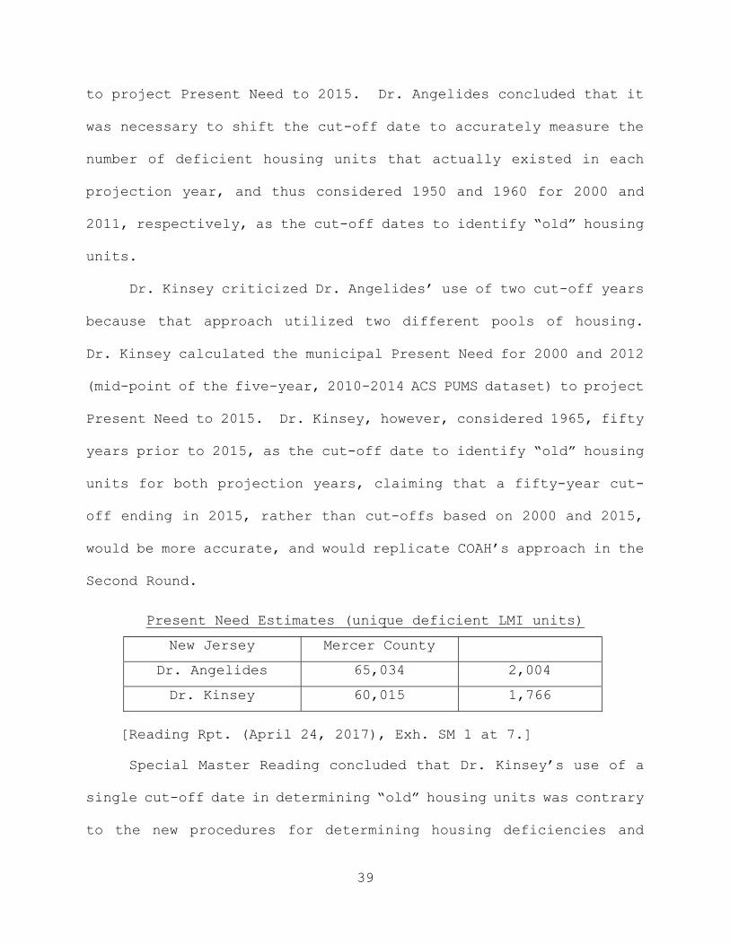
Present Need Estimates (unique deficient LMI units)
New Jersey Mercer County
Dr. Angelides 65,034 2,004
Dr. Kinsey 60,015 1,766
[Reading Rpt. (April 24, 2017), Exh. SM 1 at 7.]
Special Master Reading concluded that Dr. Kinsey’s use of a
single cut-off date in determining “old” housing units was contrary
to the new procedures for determining housing deficiencies and

40
undermined the reliability of Dr. Kinsey’s estimates. The court
agrees with Mr. Reading’s appraisal and adopts Dr. Angelides’
approach, concluding that it makes more sense to determine if a
housing unit is “old” at the time it is being counted, rather than
if it will be “old” at a particular time in the future. Notably,
this calculation of need was one of the only times that Dr.
Angelides recommended a higher need number than Dr. Kinsey.
Consequently, the Present Need obligations adopted by the court
are reflected in the following chart:
Present Need 2015
New Jersey 65,034
Region 4 7,195
Mercer County 2,004
Princeton 80
West Windsor Township 132
3. Calculate Regional Prospective Need
The FHA defines Prospective Need as “a projection of housing
needs based on development and growth which is reasonably likely
to occur in a region or a municipality . . .” N.J.S.A. 52:27D-
304(j). Prospective Need is a number reflecting the estimated
incremental change in LMI households within each region during the
Prospective Need period. Both Drs. Angelides and Kinsey agreed on
a Prospective Need period from July 1, 2015 through June 30, 2025,
and accepted the six regions as delineated by COAH, with Mercer
County as part of Region 4, along with Ocean and Monmouth Counties.
41
To determine regional Prospective Need, the experts: (1)
predicted the regional population growth over the Prospective Need
period; (2) estimated the proportion of that population living in
households; (3) estimated the number of households associated with
that population; (4) estimated the growth of LMI households during
the Prospective Need period; (5) removed households (primarily
senior citizens) with significant assets from Prospective Need
calculations (Dr. Angelides only); and (6) calculated the regional
Prospective Need as the incremental change between the estimate of
LMI households at the beginning and end of the Prospective Need
period.
a. Predict Population Growth
To estimate the incremental affordable housing need over the
ten-year Prospective Need period first requires a projection of
population growth over that period. This projection is a critical
starting point for the methodology because it is a driver for the
steps with the greatest impact on need that follow. That explains
why there was extensive testimony about population statistics and
datasets from the experts, and likely explains why the parties
diverged in their projections, with the municipalities advocating
for lower population growth than FSHC during the Prospective Need
period.
Indeed, this first step in the Prospective Need methodology
vividly demonstrates the complexities involved in just one step of
42
the model. As explained below, COAH changed the datasets it used
from the First Round to the Second Round, used various datasets in
the three iterations of the Third Round, and discovered that its
past projections had been either too low or too high when the
projection periods ended. There was extensive demographic
testimony and evidence provided to the court, including updated
data that had not been included in either model developed by the
experts, but was used to support particular choices of datasets.
To say the court had to maneuver through a metaphorical minefield
to select a population projection for the Third Round is not an
understatement. The experts did agree in testimony, however, that
making population estimates is “fraught with uncertainty,”
“incredibly imprecise,” and essentially a “risky business.” And
the court had to undertake this difficult task without testimony
from any expert demographer or clear guidance from COAH, which --
as noted above -- had used different datasets in the First and
Second Round rules and the various iterations of the Third Round
rules.
All of the experts admitted that COAH relied primarily in the
Prior Rounds upon population projections from the New Jersey
Department of Labor (NJDOL) and its successor, the New Jersey
Department of Labor and Workforce Development (NJLWD). The First
Round used only the population estimates of the Historic Migration
Model (HMM), while the Second Round averaged HMM estimates with
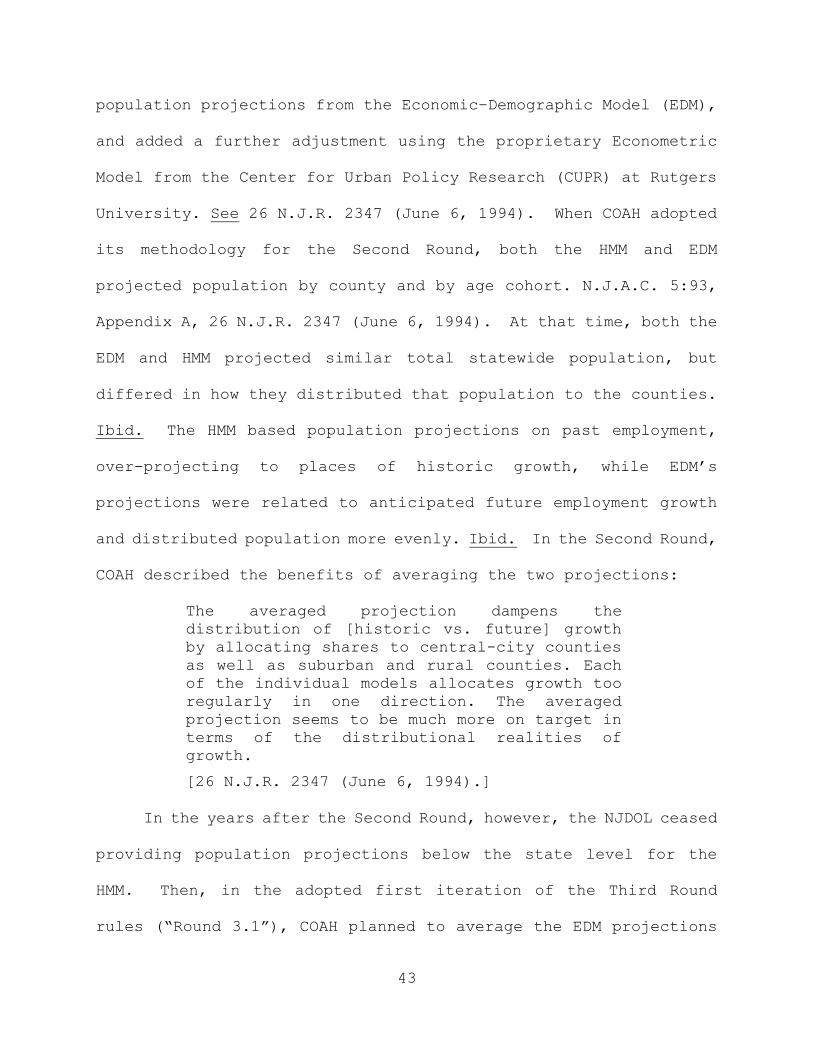
43
population projections from the Economic–Demographic Model (EDM),
and added a further adjustment using the proprietary Econometric
Model from the Center for Urban Policy Research (CUPR) at Rutgers
University. See 26 N.J.R. 2347 (June 6, 1994). When COAH adopted
its methodology for the Second Round, both the HMM and EDM
projected population by county and by age cohort. N.J.A.C. 5:93,
Appendix A, 26 N.J.R. 2347 (June 6, 1994). At that time, both the
EDM and HMM projected similar total statewide population, but
differed in how they distributed that population to the counties.
Ibid. The HMM based population projections on past employment,
over-projecting to places of historic growth, while EDM’s
projections were related to anticipated future employment growth
and distributed population more evenly. Ibid. In the Second Round,
COAH described the benefits of averaging the two projections:
The averaged projection dampens the distribution of [historic vs. future] growth by allocating shares to central-city counties as well as suburban and rural counties. Each of the individual models allocates growth too regularly in one direction. The averaged projection seems to be much more on target in terms of the distributional realities of growth.
[26 N.J.R. 2347 (June 6, 1994).]
In the years after the Second Round, however, the NJDOL ceased
providing population projections below the state level for the
HMM. Then, in the adopted first iteration of the Third Round
rules (“Round 3.1”), COAH planned to average the EDM projections
44
with a second set of estimates from the three Metropolitan Planning
Organizations (MPO) of the State, noting that “both [the MPO and
NJDOL] projections generously state the growth anticipated for the
period.” N.J.A.C. 5:94; App. A, 75. Subsequently, in the un-
adopted third iteration of the Third Round rules (“Round 3.3”),
COAH planned to rely solely on the EDM, stating that, “The
procedure employed in this analysis is to use the output of the
[EDM]. The [EDM] forecasts the future, and is the preferred model
by the State.” 46 N.J.R. 952 (June 2, 2014).
Neither Dr. Angelides nor Dr. Kinsey followed the Second Round
exactly, as it was impossible to do so with the HMM no longer
providing county or age group data, and without CUPR’s proprietary
Econometric Model, which was not reproducible for use by the
experts who designed methodologies for the court. Instead, Dr.
Angelides averaged population projections from the EDM and HMM as
in the Second Round, but modified that Round’s approach by
averaging the HMM and EDM statewide population projections and
then applying EDM’s county and age cohort distributions to the
statewide average to yield averaged projections by county and age
cohort combinations.
While Dr. Angelides defended his approach as the most faithful
to COAH’s preferred method in the Second Round, he also presented
significant data to convince the court to endorse his approach
over that of Dr. Kinsey, relying on recent statistics to show that
45
New Jersey’s population growth has slowed considerably in the last
few years. Since his approach produced estimates that were the
lower of the two, Dr. Angelides urged the court to adopt his
projections as the demonstrably more accurate ones. To make his
point, Dr. Angelides presented new inter-censal 2016 Census Bureau
population estimates, which are released annually and update the
prior years’ estimates back to the previous decennial census. The
new estimates showed slower statewide population growth for the
2010-2015 period than was depicted in the 2015 Census updates.
Dr. Angelides also cited newly released 2016 NJLWD data to
demonstrate that both the HMM and EDM projections had overestimated
statewide population growth over the 2000-2016 period, contending
that his averaged approach more closely tracked the 2016 population
estimates than Dr. Kinsey’s projections.
Dr. Kinsey’s approach utilized a combination of census
population data and EDM population projections. For 2015, Dr.
Kinsey relied on population estimates published by the United
States Census Bureau as of July 1, 2015, while his 2025 population
estimates were derived from the EDM projections. Dr. Kinsey
asserted that incorporating census population data at the
beginning of the Prospective Need period utilized the “most up-
to-date available data” even though he acknowledged that COAH had
not used different data sources for the beginning and end of the
Prospective Need period in the Second Round. So, despite his

46
avowed adherence to COAH’s Second Round methodology, Dr. Kinsey
did, in this instance and in a few other steps, recommend some
deviations from COAH’s approach in the Second Round. Indeed, even
though COAH in the un-adopted Round 3.3 rules relied on the EDM,
it made no mention of utilizing Census data in this step and
generally avoided inter-mixing data sources for population
projections in the manner recommended to this court by Dr. Kinsey.
Special Master Reading was troubled by Dr. Kinsey’s inter-
mixing of census population estimates and EDM population
projections to calculate population growth during the Prospective
Need period. Reading Rpt. (April 24, 2017), Exh. SM 1 at 8-11. Mr.
Reading concluded that, for the sake of data consistency, Dr.
Kinsey should have used the same EDM population estimate source
for both 2015 and 2025. He noted that Dr. Kinsey’s inter-mixing of
data inappropriately skewed his results, significantly increasing
projected population growth above both the approach used by Dr.
Angelides, and the EDM-only approach that COAH had used in Round
3.3. Mr. Reading provided statistics from which the following
chart was prepared to compare the three methods:
47
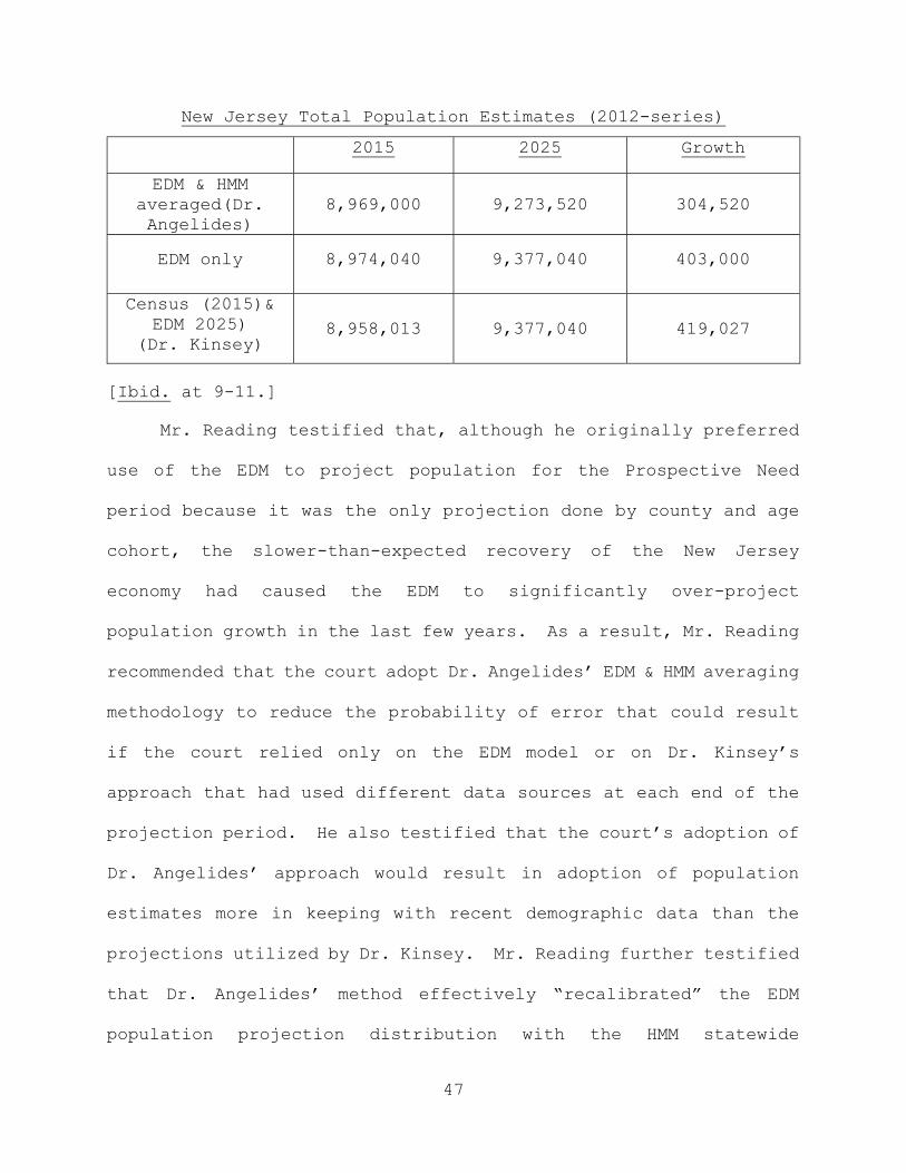
New Jersey Total Population Estimates (2012-series)
2015 2025 Growth
EDM & HMM averaged(Dr. Angelides)
8,969,000 9,273,520 304,520
EDM only 8,974,040 9,377,040 403,000
Census (2015)& EDM 2025)
(Dr. Kinsey) 8,958,013 9,377,040 419,027
[Ibid. at 9-11.]
Mr. Reading testified that, although he originally preferred
use of the EDM to project population for the Prospective Need
period because it was the only projection done by county and age
cohort, the slower-than-expected recovery of the New Jersey
economy had caused the EDM to significantly over-project
population growth in the last few years. As a result, Mr. Reading
recommended that the court adopt Dr. Angelides’ EDM & HMM averaging
methodology to reduce the probability of error that could result
if the court relied only on the EDM model or on Dr. Kinsey’s
approach that had used different data sources at each end of the
projection period. He also testified that the court’s adoption of
Dr. Angelides’ approach would result in adoption of population
estimates more in keeping with recent demographic data than the
projections utilized by Dr. Kinsey. Mr. Reading further testified
that Dr. Angelides’ method effectively “recalibrated” the EDM
population projection distribution with the HMM statewide
48
projection, which was the lower of the two approaches, and thus
was the more accurate estimate when compared to recent New Jersey
population trends. While Dr. Kinsey was critical of the
recalibration done by Dr. Angelides because it could introduce
error into the model, Mr. Reading testified that such
interpolations were commonly employed in statistical analysis and
had been used by both experts in other parts of their fair share
methodologies.
The court concurs with Mr. Reading’s recommendation and will
adopt the approach utilized by Dr. Angelides, but updated to use
the 2016 HMM and EDM projections prepared by NJLWD, which are now
available. Notably, as the trial progressed, new data was
produced. Indeed, as of the end of the trial, almost two years —
- or 20 percent -- of the Prospective Need period of July 2015 to
June 2025 had elapsed. During that time, NJLWD released updated
models. In addition, while Dr. Kinsey had cited the population
projections of the Rutgers Economic Advisory Service (R/ECON) to
support his prediction of population growth of almost 42,000
annually, Dr. Powell testified that Rutgers had subsequently
reduced its population growth projection to approximately 27,000
a year, far less than the growth advocated by Dr. Kinsey, and
closer to the estimate used by Dr. Angelides. Moreover, although
there was testimony from Dr. Kinsey cautioning the court about
relying on population swings over a short period of time, the
49
decreased rate of growth in New Jersey since the recession started
in 2008 has continued for close to ten years despite an economic
upturn and cannot be ignored by the court.
While both Dr. Kinsey and Mr. Bernard urged the court to
ignore the recent data and employ the EDM, that model was shown to
have over-projected population in the recent past to a
significantly greater degree than the HMM. Ignoring that reality
would contradict the direction of the Supreme Court to use the
best available and most recent data. In addition, Dr. Kinsey did
not utilize the same population data source at both end points of
his projection, but inter-mixed data in a way not supported by any
past COAH practice and one leading to significant inflation of
population growth during the Prospective Need period. As noted by
Mr. Reading, in making population projections, results can be
significantly skewed by even seemingly small deviations caused by
utilizing different data sources at the endpoints.
Averaging the HMM and EDM as COAH did in the Second Round
thus makes the most sense based on the record, although the court
acknowledges that even averaging is not immune from error due to
the need to recalibrate the HMM using EDM population distributions,
as well as the inherent speculative nature of all population
projections. Given the results of the averaging, however, which
better reflect historical data from at least the last ten years,
the court finds the approach of Dr. Angelides to be preferable at
50
this point in time. While Mr. Reading noted the availability of
other population projection sources, such as R/ECON, he concluded
that there was insufficient evidence in the record to deviate from
COAH’s primary reliance on the EDM and HMM in Prior Rounds. The
court is also reluctant to adopt a data source used neither by
COAH nor by any expert who designed a methodology for judicial
review.
Mr. Bernard, after acknowledging the imprecision of all
population projections, simply asserted that all COAH could do
when faced with the similar uncertainty inherent in making
estimates of population growth over a period of years was to do
its best. That is what the court has endeavored to do here in the
face of no completely satisfactory alternative. Thus, the court
agrees with Mr. Reading and endorses Dr. Angelides’ approach to
estimating population growth in the Prospective Need period by
averaging EDM and HMM projections, following as closely as possible
what COAH had done in the Second Round. Since NJLWD released
updated EDM and HMM models after Dr. Angelides prepared his model,
the court directs that the newly updated, 2014-based NJLWD
projections released in 2016 be used in the methodology, following
Mr. Reading’s recommendation. Reading Rpt. (April 24, 2017), Exh.
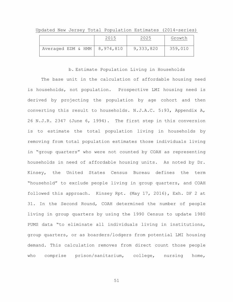
SM 1 at 65. The court thus adopts the following aggregated New
Jersey total estimated population for the Third Round:
51
Updated New Jersey Total Population Estimates (2014-series)
2015 2025 Growth
Averaged EDM & HMM 8,974,810 9,333,820 359,010
b. Estimate Population Living in Households
The base unit in the calculation of affordable housing need
is households, not population. Prospective LMI housing need is
derived by projecting the population by age cohort and then
converting this result to households. N.J.A.C. 5:93, Appendix A,
26 N.J.R. 2347 (June 6, 1994). The first step in this conversion
is to estimate the total population living in households by
removing from total population estimates those individuals living
in “group quarters” who were not counted by COAH as representing
households in need of affordable housing units. As noted by Dr.
Kinsey, the United States Census Bureau defines the term
“household” to exclude people living in group quarters, and COAH
followed this approach. Kinsey Rpt. (May 17, 2016), Exh. DF 2 at
31. In the Second Round, COAH determined the number of people
living in group quarters by using the 1990 Census to update 1980
PUMS data “to eliminate all individuals living in institutions,
group quarters, or as boarders/lodgers from potential LMI housing
demand. This calculation removes from direct count those people
who comprise prison/sanitarium, college, nursing home,

52
boarders/boarding homes, and other related populations.” N.J.A.C.
5:93, Appendix A, 26 N.J.R. 2343 (June 6, 1994).
Notably, COAH excluded individuals living in group quarters
from people living in households even though COAH provided
compliance credits to municipalities for the creation of
“alternative living arrangements.” COAH defined that term in
N.J.A.C. 5:93-1.1 as structures “in which households live in
distinct bedrooms, yet share kitchen and plumbing facilities,
central heat and common areas.” Included in the definition were
boarding houses, residential care facilities, and group homes for
developmentally disabled or mentally ill persons. Ibid. N.J.A.C.
5:93-5.8 allows municipalities to obtain compliance credits for
alternative living arrangements, with credits being awarded for
the number of bedrooms created. While there is an inconsistency
in this approach in terms of excluding individuals living in group
quarters from total population living in households while
simultaneously awarding bonus credits for the creation of bedrooms
for some of the same people who reside in alternative living
arrangements, no expert recommended including people living in
group quarters in the determination of affordable housing need at
this time, deeming such a consideration to be a policy judgment
better left to an administrative agency. The court reluctantly
agrees with this approach. Consequently, the court will deduct
the estimate of people living in group quarters from the total
53
population living in households as part of its fair share
methodology, although an administrative agency should consider in
the future including in its population projections the people
housed in alternative living arrangements, since increasing the
bedrooms available in such units can generate bonus credits for
municipalities in the compliance process.
The estimation of the number of people living in group
quarters does not raise a significant methodological dispute here
because Dr. Angelides and Dr. Kinsey recommended similar
percentages to deduct from total population to account for those
individuals living in group quarters. Indeed, their percentages
differed by negligible amounts: 2.08 percent compared to 2.09
percent statewide, respectively, for 2015, and 2.13 percent
compared to 2.14 percent statewide for 2025. Reading Rpt. (April
24, 2017), Exh. SM 1 at 12-13. While the percentages were similar,
application of them to the substantially differing total
population estimates recommended by each expert produced divergent
results. Because of the negligible difference between Drs.
Angelides’ and Kinsey’s percentage estimates of population living
in group quarters, however, and to maintain consistency with the
prior step where the court accepted Dr. Angelides’ population
estimates, the court will accept Dr. Angelides’ calculated values
of 2.08 percent and 2.13 percent here. When the ratio calculated
for group quarters is applied to the total population endorsed in
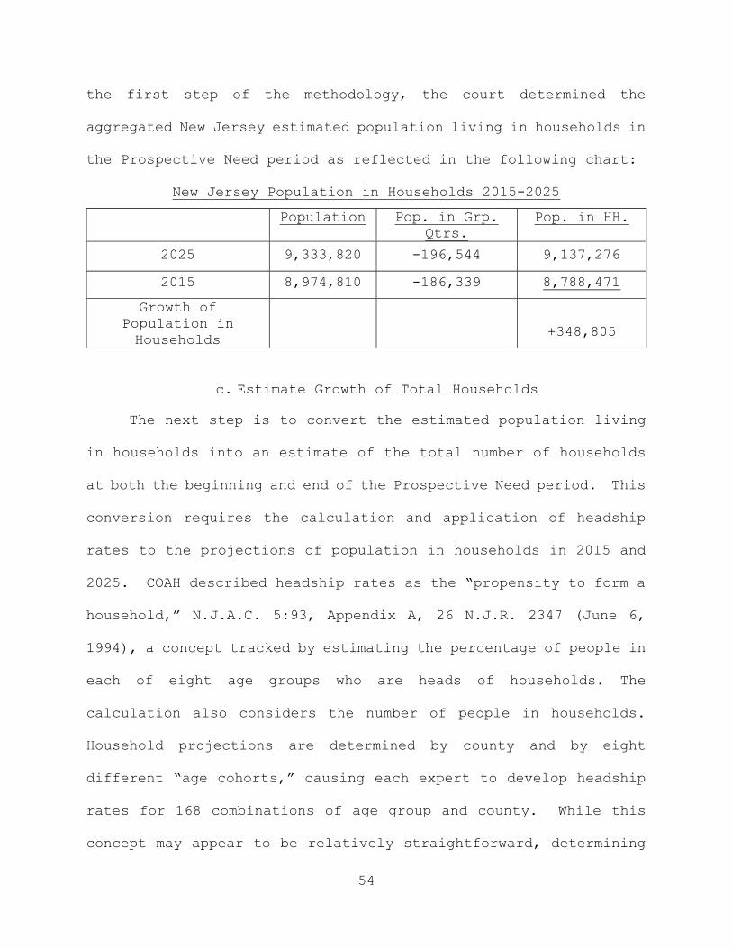
54
the first step of the methodology, the court determined the
aggregated New Jersey estimated population living in households in
the Prospective Need period as reflected in the following chart:
New Jersey Population in Households 2015-2025
Population Pop. in Grp. Qtrs.
Pop. in HH.
2025 9,333,820 -196,544 9,137,276
2015 8,974,810 -186,339 8,788,471
Growth of Population in Households
+348,805
c. Estimate Growth of Total Households
The next step is to convert the estimated population living
in households into an estimate of the total number of households
at both the beginning and end of the Prospective Need period. This
conversion requires the calculation and application of headship
rates to the projections of population in households in 2015 and
2025. COAH described headship rates as the “propensity to form a
household,” N.J.A.C. 5:93, Appendix A, 26 N.J.R. 2347 (June 6,
1994), a concept tracked by estimating the percentage of people in
each of eight age groups who are heads of households. The
calculation also considers the number of people in households.
Household projections are determined by county and by eight
different “age cohorts,” causing each expert to develop headship
rates for 168 combinations of age group and county. While this
concept may appear to be relatively straightforward, determining
55
the headship rates to utilize in the affordable housing model once
again thrust the court into a morass of conflicting approaches,
each of which had positive and negative aspects. Again, no
approach was perfect, and none impressed the court as significantly
superior to the others. As was true in selecting a population
projection, following COAH practice in regard to headship rates
was challenging. Not only did COAH utilize different approaches in
Prior Rounds, but it created certain ambiguities in the Second
Round that caused at least two of the experts to refer to the
Second Round application of headship rates as a “black box.”
Despite these difficulties, the court reviewed the record and
selected the headship rates it deemed preferable as part of the
Prospective Need methodology for use in the Third Round.
In Appendix A to the Second Round Rules, 26 N.J.R. 2342-2353
(June 6, 1994), which Mr. Bernard testified was prepared by COAH
consultant Dr. Robert Burchell of Rutgers University, COAH stated
in a section entitled “Household Projections” that, “Headship
rates are determined by age group and county in New Jersey in 1990
and extended into the future at one-half the rate of change
observed from 1980 to 1990.” 26 N.J.R. 2347 (June 6, 1994). This
statement endorses use of a trend line in headship rates developed
from the ten-year period between the two most recent decennial
censuses and applied to population projections to determine the
number of total households in the Prospective Need period.
56
Apparently, however, COAH had used flat headship rates in the First
Round, and Appendix A from the Second Round stated in a section
entitled “Prospective Need” that, “Both the population cohorts for
the base year (1993) and the projection year (1999) are multiplied
by 1990 New Jersey county-specific headship rates by age cohort,”
suggesting that a flat headship rate was utilized instead of a
trend line. Given the explicit language in the section governing
“Household Projections,” however, the consensus among the experts
was that COAH likely had developed a trend line and used one-half
of the rate of change observed between 1980 and 1990 to calculate
its headship rates in the Second Round. Notably, the descriptive
language in Appendix A did not state clearly whether the trend
line started in 1990, the year of the most recent decennial census,
or in 1993, the beginning of the Prospective Need period for the
Second Round. Mr. Bernard testified that COAH relied upon its
consultant, Dr. Burchell, for this aspect of the methodology and
–- given the conflicting language in Appendix A -- Mr. Bernard
could not be sure as to the exact approach utilized in the Second
Round to determine headship rates.
The complexity inherent in determining headship rates is
underscored by the fact that FSHC retained a national expert to
supplement testimony from Dr. Kinsey regarding this issue. This
aspect of the model was the only area where FSHC looked to an
expert other than Dr. Kinsey. FSHC retained Mr. McCue from the

57
Joint Center for Housing Studies at Harvard University (“Joint
Center”) to provide testimony to the court regarding headship
rates. While FSHC likely expected Mr. McCue to support Dr.
Kinsey’s use of flat headship rates in the Prospective Need period,
the Joint Center changed its approach to using a trend line after
Dr. Kinsey finished his model. As a result, Mr. McCue offered
rationales for alternative approaches, one using a flat headship
rate and the other using a trend line. Although Dr. Angelides had
used a trend line in determining his headship rates, Mr. McCue
objected to Dr. Angelides starting his trend line in 2014 instead
of in 2010, the year of the most recent decennial census. Starting
in 2014 resulted in lower headship rates over the Prospective Need
period than would be the case if the trend were started in 2010.
The court thus had to sort out the different approaches advocated
by the experts, while remaining cognizant of their admonition that
even small deviations in headship rates can translate into
significant differences in total households —- a key building block
in the methodology, and one that has a major impact on the
determination of need. Indeed, the court was cautioned that an
error in this part of the model would be magnified throughout the
rest of the methodology.
Before looking more deeply into the different approaches
recommended by the experts, the court will turn to aspects of the
methodology where they agree. Notably, while the population
58
estimates for the model were based on NJLWD projections, all of
the experts developed their headship rates using datasets prepared
by the United States Census Bureau. They used population
statistics from the two most recent decennial censuses —- 2000 and
2010 -- finding those datasets to be the most reliable ones
available. Since the Prospective Need period began in 2015, Drs.
Angelides and Kinsey relied upon the most recent household data
available when they prepared their reports —- the 2014 ACS -- a
Census Bureau product based on a sampling of households and not a
complete population count. Although the ACS was not available
during the Second Round, Drs. Angelides and Kinsey agreed that it
was an appropriate dataset to use in developing headship rates for
the Third Round. Notably, however, Mr. McCue, who identified
himself as a housing demographer, testified that it is well known
that although the ACS reports population estimates similar to those
reported in the decennial Census, the ACS significantly
underreports headship rates throughout the country. To correct
for this acknowledged aberration, Drs. Angelides and Kinsey
adjusted the 2014 ACS headship rates with a “calibration factor”
calculated by comparing 2010 Census-derived and 2010 ACS-derived
headship rates and adjusting the ACS data to reflect the Census-
derived headship rates. While some of the experts voiced concern
at various steps of the model concerning manipulating data, the
59
calibration done in this step showed that some recalibration of
data is well-recognized when circumstances require adjustments.
After recalibrating the ACS data, Dr. Angelides then followed
the explicit language in Appendix A of the Second Round by
calculating a trend line at one-half the change in headship rates
between the two most recent decennial Census years of 2000 and
2010 and then projecting the trend to 2025 from the calibrated
2014 ACS headship rate, for each New Jersey county and age cohort.
From these trend lines, Dr. Angelides determined aggregated
statewide 2015 and 2025 headship rates of 37.04 percent and 37.45
percent, respectively.
Although Dr. Kinsey professed strong allegiance to the Second
Round practices of COAH throughout the trial, he deviated from the
apparent Second Round methodology by holding the calibrated 2014
ACS headship rates steady from 2014 into 2015 and 2025. Dr. Kinsey
justified this deviation from the Second Round by citing an annual
study from the Joint Center for 2015, which used flat headship
rates. Although Dr. Kinsey held headship rates constant in his
projection, growth rate variations between county and age cohort
pairs yielded increasing aggregated headship rates of 37.11
percent and 37.71 percent for 2015 and 2025 respectively. Reading
Rpt. (August 31, 2016), Exh. SM 4 at 36.
Drs. Angelides and Kinsey made the following recommendations
to the court:
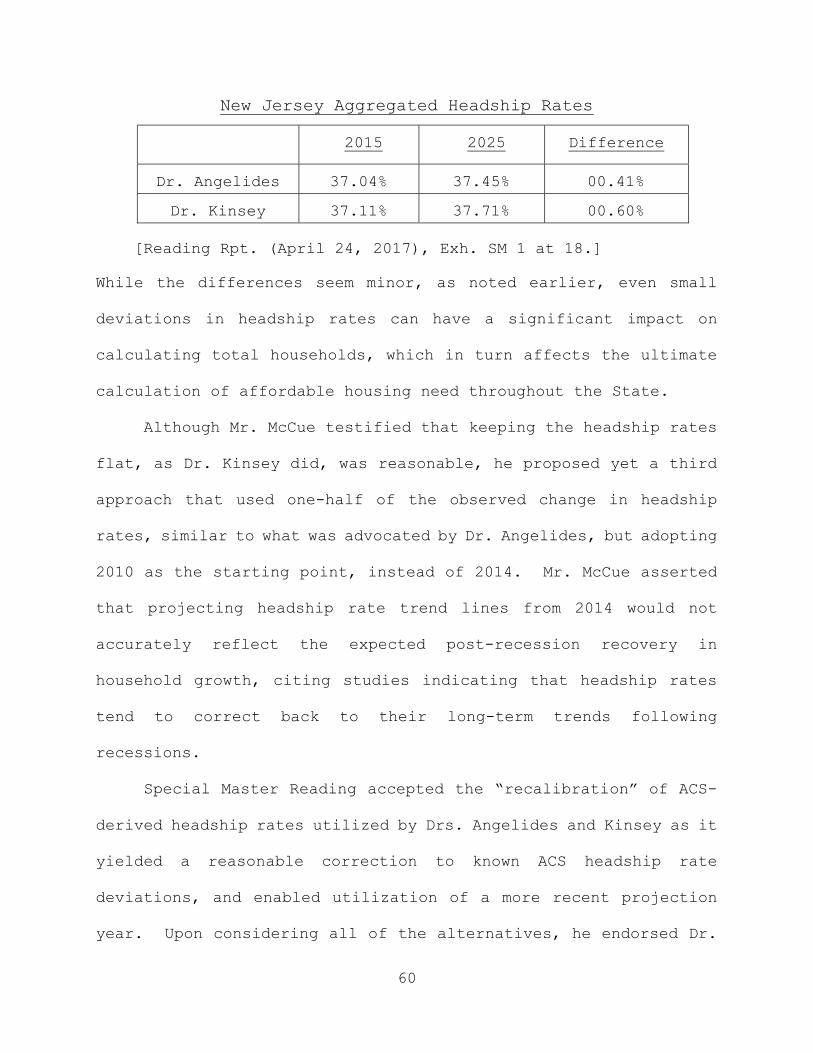
60
New Jersey Aggregated Headship Rates
2015 2025 Difference
Dr. Angelides 37.04% 37.45% 00.41%
Dr. Kinsey 37.11% 37.71% 00.60%
[Reading Rpt. (April 24, 2017), Exh. SM 1 at 18.]
While the differences seem minor, as noted earlier, even small
deviations in headship rates can have a significant impact on
calculating total households, which in turn affects the ultimate
calculation of affordable housing need throughout the State.
Although Mr. McCue testified that keeping the headship rates
flat, as Dr. Kinsey did, was reasonable, he proposed yet a third
approach that used one-half of the observed change in headship
rates, similar to what was advocated by Dr. Angelides, but adopting
2010 as the starting point, instead of 2014. Mr. McCue asserted
that projecting headship rate trend lines from 2014 would not
accurately reflect the expected post-recession recovery in
household growth, citing studies indicating that headship rates
tend to correct back to their long-term trends following
recessions.
Special Master Reading accepted the “recalibration” of ACS-
derived headship rates utilized by Drs. Angelides and Kinsey as it
yielded a reasonable correction to known ACS headship rate
deviations, and enabled utilization of a more recent projection
year. Upon considering all of the alternatives, he endorsed Dr.
61
Angelides’ approach, but adjusted it to project from 2015, the
beginning of the Prospective Need period, instead of 2014, because
more recent data was now available that coincided with the start
of the period. Mr. Reading also endorsed use of the trend line
over flat rates as consistent with what he believed COAH had done
in the Second Round. In addition, Mr. Reading preferred use of
a trend line based on one-half of the observed change because it
mitigated the extreme effects that could arise from relying on an
atypical time period, such as 2000 to 2010, which included three
distinct economic trends: pre-recession, recession, and early
recovery.
In support of his endorsement of Dr. Angelides’ trend line
approach updated to use 2015 ACS recalibrated data, Mr. Reading
cited the fact that the Joint Center, relied upon by Dr. Kinsey as
having used flat rate headship projections, had recently returned
to relying upon a trend line calculated with one-half the rate of
change. Mr. Reading rejected Mr. McCue’s recommendation to start
the trend line in 2010, however, because Mr. McCue had based his
opinion on nationwide data concerning recovery from the recession,
which data was inconsistent with the much slower recovery being
experienced in New Jersey. While noting that COAH’s Second Round
rules were unclear as to whether COAH had projected its one-half
headship rate trend line from the 1990 decennial Census year, or
had instead used 1993, the beginning of the Second Round
62
Prospective Need period, Mr. Reading endorsed starting the trend
line at the beginning of the Prospective Need period as making
more sense in the current circumstances given recent economic
trends in New Jersey and the availability of actual data for 2015.
In determining the appropriate methodology for this step, the
court must choose both a proper projection starting year and
headship rate approach. First, the court agrees with Mr. Reading
that it makes sense to project headship rates from the beginning
of the Prospective Need period using newly available, although
appropriately recalibrated ACS data, a dataset that was not
available to COAH in the Second Round. The court prefers use of
a trend line over a flat rate because the record strongly suggests
that COAH followed this procedure in the Second Round and the Joint
Center recently endorsed a trend line approach. Indeed, when
pressed on cross-examination, Mr. McCue expressed a slight
preference at this point in time for developing a trend line using
one-half the observed change in headship rates, unsurprisingly
endorsing the recent change implemented by the Joint Center in its
national housing study.
The selection of the starting point for the trend line
presents a thornier issue because the reasons supporting the
choices made by the experts did not point to a definite answer.
Nor was there explicit guidance from COAH to follow. But it did
appear that Mr. McCue’s recommendation was based on a national
63
rebound from the recession that has not been replicated in New
Jersey, which is recovering at a slower rate. Mr. McCue admitted
to not being an economist and to a general lack of familiarity
with both recent economic trends in New Jersey and COAH practice.
He did acknowledge, however, that headship rates in New Jersey
were abnormally low and that his own trend line had anticipated
more significant growth than had actually occurred in the State
based on recent data. He also stated that increases in headship
rates lag behind improvement in other economic areas such as
employment following a recession, suggesting to the court that the
starting point for the trend line recommended by Mr. Reading as an
adjustment to the one endorsed by Dr. Angelides offers the best
alternative based on recent economic conditions in New Jersey.
Indeed, the court is not persuaded based on the record that New
Jersey’s headship rates will recover to pre-recession levels by
the end of the Prospective Need period, as assumed by Mr. McCue,
who recommended projecting from 2010. In addition, COAH noted in
the Second Round that headship rate growth is typically greatest
in the younger age groups, 26 N.J.R. 2347 (June 6. 1994), and there
was testimony in the record that New Jersey has more young adults
living with their parents than any other state in the country.
These considerations also persuaded the court to reject Mr. McCue’s
trend line. The court further notes that while Mr. McCue is a
national expert in headship rates, Mr. Reading is much more

64
familiar with economic trends in New Jersey, so that his
endorsement of starting the trend line in 2015 based on the current
state of the New Jersey economy carried greater weight.
The court also concurs with Mr. Reading that a one-half
headship rate projection is appropriate to account for the
uncertainties presented by the period following the Great
Recession. Indeed, the court finds a one-half headship rate trend
line, projected from 2015, to be reasonable as it strikes an
appropriate balance between Mr. McCue’s proposal, which too
optimistically assumes household trends will recover by the end of
the Prospective Need period to where they would have been but for
the recession, and Dr. Kinsey’s flat headship rate approach that
completely disregards prevailing housing trends. Moreover, as
noted by Mr. McCue, there is only a slight difference between the
headship rates endorsed by Dr. Angelides and Dr. Kinsey, despite
their dissimilar approaches, while the difference between those
headship rates and the ones produced by Mr. McCue’s alternate trend
line projecting from 2010 was much more pronounced.
The court is thus much more comfortable selecting Dr.
Angelides’ trend line, which resulted in headship rates closer to
the ones advocated by Dr. Kinsey, than it is endorsing Mr. McCue’s
trend line, which produced more aberrant results. The court
consequently will follow Mr. Reading’s recommendation and adopt
Dr. Angelides’ trend line using one-half the observed rate of

65
change in headship rates when projecting 2015 and 2025 headship
rates, but will project from calibrated 2015 ACS-derived headship
rates, as suggested by Mr. Reading. After reviewing all of the
alternatives, this one is the best. The court also notes that
since it endorsed the population projection approach advocated by
Dr. Angelides and Mr. Reading, the headship rates selected by the
court will be applied to those projections. The results of this
analysis, showing the aggregated New Jersey estimated growth in
total households in the Prospective Need period, are reflected in
the following chart:
New Jersey Total Households 2015-2025
Headship
Rate
Population in
HH. Total HH.
2025 37.63% 9,137,276 3,438,417
2015 37.11% 8,788,471 3,261,626
Total Household Growth +176,791
d. Estimate LMI household growth during the Prospective Need period
Once the projected numbers of total households at the
beginning and end of the Prospective Need period have been
determined, the next step is to estimate the proportion of those
households that qualify as LMI at each point in time. Having those
estimates will allow the court to determine the growth of LMI
households during the period (“LMI Household Growth”), another key
factor in the development of the fair share methodology. In the

66
Prior Rounds, COAH accomplished this step by calculating and then
applying the ratios of LMI households to total households (“LMI
Household Ratio”) by county and age cohort, and then aggregating
the results to the regions. Prior Round rules do not reveal the
precise calculations COAH used in this step, although some guidance
can be gleaned from COAH’s statements. In evaluating Drs.
Angelides’ and Kinsey’s approaches, the court has identified two
distinct sub-steps that require consideration: 1) selection of
income qualification data to use in calculating LMI Household
Ratios, and 2) how LMI Household Ratios are applied to Total
Household projections to estimate LMI Household Growth in the
Prospective Need period. The court discusses each in turn.
i. Income Qualification Data Used in Determining LMI Household Ratio Calculation
In the Prior Rounds, COAH calculated LMI Household Ratios in
this step of the methodology by utilizing income grids it developed
from median income thresholds established by the Federal
Department of Housing and Urban Development (HUD) for its
affordable housing programs, as authorized in the FHA:
Moderate income housing means housing affordable according to [HUD] or other recognized standards for home ownership and rental costs and occupied or reserved for occupancy by households with a gross household income equal to more than 50% but less than
67
80% of the median gross household income for households of the same size within the region in which the housing is located.
[N.J.S.A. 52:27D-304(d).]
By incorporating HUD standards into its fair share methodology,
COAH was following the suggestion of the Supreme Court in Mount
Laurel II, 92 N.J. at 220-221, fn. 8, which acknowledged the
benefit of incorporating well-accepted federal standards into New
Jersey’s affordable housing program.
COAH’s Second Round rule-making expressly noted that the
agency was using HUD income limits, based upon household size, to
establish the LMI income thresholds from which LMI Household Ratios
were determined:
Total households for [1993 and 1999] are converted to low- and moderate-income households by carrying forward the income characteristics of all households in 1990 to 1993 and 1999 by age cohort. Low- and moderate-income households are sorted by applying the Section 8 household size/income qualification criteria that were used in 1992 . . .
[N.J.A.C. 5:93, Appendix A, 26 N.J.R. 2347 (June 6, 1994).]
COAH used HUD median income data from each county in New
Jersey to calculate a weighted average median income for a family
of four for each region. N.J.A.C. 5:93-7.4(a). COAH then
calculated median incomes for households larger and smaller than
four by applying multipliers used by HUD, as shown for Region Four
in 2014:
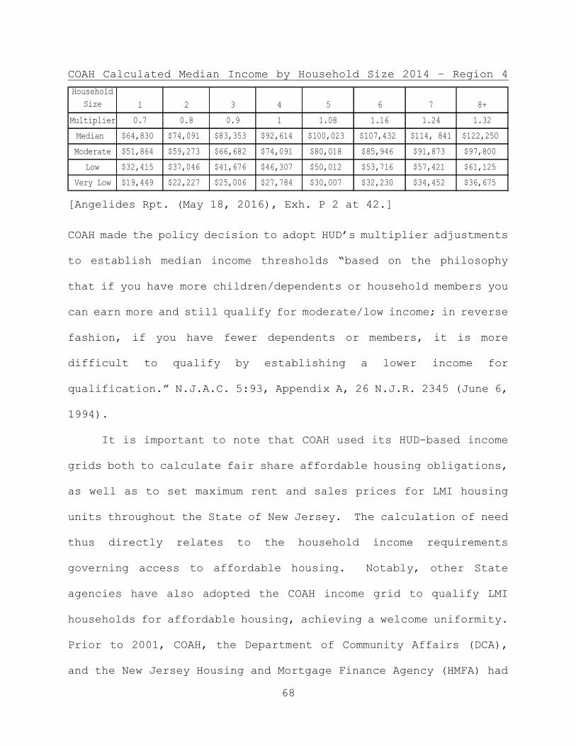
68
COAH Calculated Median Income by Household Size 2014 – Region 4
[Angelides Rpt. (May 18, 2016), Exh. P 2 at 42.]
COAH made the policy decision to adopt HUD’s multiplier adjustments
to establish median income thresholds “based on the philosophy
that if you have more children/dependents or household members you
can earn more and still qualify for moderate/low income; in reverse
fashion, if you have fewer dependents or members, it is more
difficult to qualify by establishing a lower income for
qualification.” N.J.A.C. 5:93, Appendix A, 26 N.J.R. 2345 (June 6,
1994).
It is important to note that COAH used its HUD-based income
grids both to calculate fair share affordable housing obligations,
as well as to set maximum rent and sales prices for LMI housing
units throughout the State of New Jersey. The calculation of need
thus directly relates to the household income requirements
governing access to affordable housing. Notably, other State
agencies have also adopted the COAH income grid to qualify LMI
households for affordable housing, achieving a welcome uniformity.
Prior to 2001, COAH, the Department of Community Affairs (DCA),
and the New Jersey Housing and Mortgage Finance Agency (HMFA) had
Household Size 1 2 3 4 5 6 7 8+
Multiplier 0.7 0.8 0.9 1 1.08 1.16 1.24 1.32
Median $64,830 $74,091 $83,353 $92,614 $100,023 $107,432 $114, 841 $122,250
Moderate $51,864 $59,273 $66,682 $74,091 $80,018 $85,946 $91,873 $97,800
Low $32,415 $37,046 $41,676 $46,307 $50,012 $53,716 $57,421 $61,125
Very Low $19,449 $22,227 $25,006 $27,784 $30,007 $32,230 $34,452 $36,675

69
adopted inconsistent and overlapping sets of rules regarding the
continuing affordability of housing constructed pursuant to the
FHA. In re Adoption of Unif. Hous. Affordability Controls, 390
N.J. Super. at 95. In 2001, HMFA established the Uniform Housing
Affordability Controls (UHAC), N.J.A.C. 5:80-26.1 to -26.26, which
were subsequently also adopted by COAH, N.J.A.C. 5:93-9.17, and
DCA, N.J.A.C. 5:43-4.10. 390 N.J. Super. at 96. UHAC created a
single regulatory scheme to be used by State and municipal
affordable housing administrators, and provided an array of new
enforcement tools to ensure compliance. Ibid. (citing 36 N.J.R.
3660 (August 16, 2004). UHAC’s restrictions on sales prices and
rents for affordable housing units are based on COAH’s income grid,
with UHAC defining median income as, “the median income by
household size for an applicable county, as adopted annually by
COAH.” N.J.A.C. 5:80-26.2.
For this step in the methodology, the experts’ approaches
differed substantially. Dr. Kinsey used an income grid in his
calculations, but because COAH had not released an updated income
grid since 2014, Dr. Kinsey updated the grid himself utilizing
what he determined to be COAH’s Prior Round methodology and the
HUD 2015 county income limits by family size. Kinsey Rpt. (May 17,
2016) Exh. DF 2 at 39. Dr. Angelides, on the other hand, rejected
COAH’s income grid, and calculated LMI Household Ratios from
mathematical median incomes, relying on the language in the FHA

70
that identified LMI households as those with gross household
incomes less than 80 percent of the median gross household income
for households of the same size within the region in which the
housing is located. N.J.S.A. 52:27D-304(c), (d). Dr. Angelides
calculated median incomes directly from the one-year 2014 ACS data
for each household size by region. He then set LMI thresholds
below 80 percent of the calculated median household incomes for
each household size by region.
Dr. Angelides criticized COAH’s methodology as resulting in
arbitrary median income thresholds that did not reflect actual,
measurable median household incomes, and asserted that they
ultimately produced LMI proportions in violation of the FHA. Dr.
Angelides noted, for example, that the COAH grid was overly
generous to one and two-person households by allowing them to
qualify for affordable housing with much higher incomes than actual
median incomes for those household sizes would allow. Dr.
Angelides asserted that his approach mitigated the statistical
anomalies inherent in the Prior Round methodology that eschewed
true median incomes in favor of the HUD-derived medians
incorporated into the COAH income grid.
Special Master Reading preferred Dr. Angelides’ approach
because it utilized precise mathematical calculations based on
actual median incomes and produced approximate 40 percent LMI
Household Ratios, consistent with the mathematical definition of

71
median when applied to the FHA. Mr. Reading disagreed with Dr.
Kinsey’s use of an income grid because the grids were developed
for the purpose of qualifying people to obtain affordable housing,
not to determine affordable housing obligations that must be met
by municipalities. Mr. Reading also expressed concern regarding
Dr. Kinsey’s use of HUD’s median incomes, because HUD had recently
changed its method for determining median incomes and was now
utilizing ACS data. However, while expressing concern that COAH
had not effectively updated its HUD-derived income grid since 2012,
Mr. Reading nonetheless testified that, despite his disagreement
with the use of an income grid for determining affordable housing
need, he accepted Dr. Kinsey’s method for updating the COAH income
grid as sound. Mr. Reading added that HUD’s new method for
determining median incomes would likely have been accepted by COAH,
were the agency still functioning. Dr. Kinsey incorporated the
new HUD procedure into the COAH-inspired grid he prepared and
utilized in his methodology.
The court rejects Dr. Angelides’ assertion that the use by
COAH and Dr. Kinsey of income grids to calculate affordable housing
obligations violates the FHA. The FHA explicitly references HUD
standards, as quoted above, and COAH repeatedly made the
unambiguous policy decision to use the same income grid for
determining affordable housing need as it used for income
qualification and for the pricing of affordable housing units.
72
Indeed, Mr. Bernard cited text from the summary of proposed changes
to COAH’s First Round rules in which COAH determined to use income
grids as a means to remedy situations where individual LMI
households that were included in need calculations could not afford
the LMI housing constructed within their region:
The Council believes that the standards set for pricing and income qualification in a region should be the same as that used to determine need. Therefore, the Council is proposing regional income standards, to eliminate such inequities, based on New Jersey income data.
[25 N.J.R. 1121 (March 15, 1993).]
The same HUD-derived income data was used in the Second Round.
N.J.A.C. 5:93, Appendix A, 26 N.J.R. 2344-2345 (June 6, 1994).
COAH’s interpretation and application of the FHA is entitled to
deference. Indeed, a long period of consistent construction by an
administrative agency in the field of its expertise should be given
great weight by the courts. Mastrobattista v. Essex County Park
Commission, 46 N.J. 138, 146 (1965); Pringle v. New Jersey Dept.
of Civil Service, 45 N.J. 329, 332-333 (1965). While the court
appreciates Mr. Reading’s fidelity to mathematical principles and
thus his preference for calculating LMI Household Ratios using
true mathematical median incomes, the court cannot accept his
recommendation in this regard. COAH repeatedly endorsed the use
of a HUD-derived grid system to determine median income thresholds,
by household size, as an important policy that linked the
73
determination of affordable housing obligations to the means of
qualifying households that could access that affordable housing.
COAH made this policy decision through the regulatory process with
public participation and judicial oversight. In addition, the
UHAC regulations now directly link the continuing affordability of
housing constructed pursuant to the FHA to the COAH income grid
for a number of State agencies. To discard the income grid at
this juncture would not only undercut established policy decisions
by COAH, but could very well lead to an imbalance between
affordable housing units made available pursuant to constitutional
requirements and LMI households that qualify to live in that
housing.
To illustrate this point, Mr. Bernard demonstrated that under
Dr. Angelides’ methodology, persons making less than $32,000 would
have trouble affording any of the LMI housing that is regulated
through the UHAC regulations. Moreover, in endorsing the use of
an income grid, as updated by Dr. Kinsey based on HUD standards
and COAH methodology, this court is following the admonition of
the Supreme Court to follow the Prior Rounds and refrain from
acting as an administrative agency charged with making policy
decisions. Indeed, in the South Brunswick methodology trial, Judge
Wolfson adopted Dr. Kinsey’s approach, citing the fact that he had
utilized COAH’s income grid. In re Twp. of S. Brunswick, 448 N.J.
Super. at 458. The court therefore accepts Dr. Kinsey’s updated

74
COAH income grid that Mr. Reading recognized as reasonable and
adopts its use in determining LMI Household Ratios in this step.
ii. Application of LMI Household Ratios
Although the court agrees with Dr. Kinsey that an updated
COAH income grid should be used to determine LMI Household Ratios,
the court cannot fully endorse his approach to determining LMI
Household Growth in the Prospective Need period using that grid
because Dr. Kinsey deviated from Prior Round methodology in the
application of those LMI Household Ratios.
COAH’s Second Round rules only briefly summarize the
calculations performed to estimate LMI Household Growth, yet the
court was able to glean valuable insights regarding the best
approach to apply from clarifying language added by COAH to the
un-adopted Round 3.3 rules, as well as from testimony given at
trial. In discussing the methodology used to estimate LMI
Household Growth during the Second Round Prospective Need period
from 1993 to 1999, COAH stated that:
Total households for [the first year and last year of the Prospective Need period] are converted to low- and moderate-income households by carrying forward the income characteristics of all households in 1990 to 1993 and 1999 by age cohort. Low- and moderate-income households are sorted by applying the Section 8 household size/income qualification criteria that were used in 1992 to a different number of households that exist in each [age] cohort in 1993 and 1999. Thus, to the degree that age cohorts are differently
75
composed and growing differently, the low- and moderate-income population will also change as it ages into the future.
[N.J.A.C. 5:93, Appendix A, 26 N.J.R. 2347 (June 6, 1994).]
Although this Second Round language suggested that the methodology
could result in significant changes in age distribution in the LMI
population during the Prospective Need period, language added in
the un-adopted Round 3.3 rules made clear as recently as 2014 that,
despite any change in the composition of the LMI population, the
methodology should still produce an overall proportion of LMI
Household Growth to Total Household Growth during the Prospective
Need period (“LMI Household Growth Rate”) of about 40 percent:
. . . to the degree that age cohorts are differently composed and growing differently, the low- and moderate-income population will also change as it ages into the future. Nonetheless, almost by definition, about 40 percent (40.622%) of household growth will be comprised of low- and moderate-income household growth.
[46 N.J.R. 953 (June 2, 2014).]
Since COAH’s proposed Round 3.3 language appeared to
fundamentally reprise this step from the Second Round methodology,
the court found this comment instructive on two points. First,
despite any variations from true mathematical median incomes
introduced by the use of income grids in these calculations, the
percent of household growth comprised of LMI households should
still be near the 40 percent that calculations using true
76
mathematical median incomes would have produced. That follows
from the definition of LMI households in the FHA that references
50 percent of 80 percent of median incomes. Secondly, COAH made
clear that the ratio of LMI Households to total households would
be “about 40 percent” despite demographic shifts in age cohorts
during the Prospective Need period. See also, In Re Adoption of
N.J.A.C. 5:94 and 5:95 By New Jersey Council on Affordable Housing,
390 N.J. Super. at 38, where the Appellate Division acknowledged
COAH’s determination that “approximately forty percent” of
household growth in the Third Round would qualify as LMI
households.
The un-adopted Round 3.3 rule-making process also added an
appendix that provided additional insights into the methodological
steps to utilize in the then Prospective Need period of 2014 to
2024. There COAH noted that the statewide LMI Household Ratio at
the end of the Prospective Need period was assumed to be the same
as the statewide LMI household ratio at the beginning of the
Prospective Need period:
The first step in understanding low- and moderate-income housing need in New Jersey is identifying the share of households with incomes below 80 percent of their regional medians – those households qualifying for housing assistance through federal and state programs. This methodology then assumes that the same portion of New Jersey’s new households

77
[in 2024] will be below 80 percent of their regional median incomes as were below 80 percent of their regional median [in 2014]…
[46 N.J.R. 982 (June 2, 2014).]
COAH further demonstrated that the constant LMI Household Ratio
that was calculated at the beginning of the Prospective Need period
would result in the same overall LMI Household Growth Rate during
the period:
According to these procedures, low- and moderate-income households represent 40.622 percent of all households in the State [as of 2014]. If 40.622 percent of the households New Jersey is expected to add between 2014 and 2024 similarly qualify for affordable housing, Rutgers’ projections imply that 62,582 additional households will qualify for affordable housing over the 10 year period.
[46 N.J.R. 984 (June 2, 2014).]
Mr. Bernard, former Executive Director of COAH, confirmed in
testimony that COAH had similarly utilized constant LMI Household
Ratios that were calculated at the beginning of the Prospective
Need period to determine LMI Household Growth in the Second Round.
Mr. Bernard further explained that LMI Household Ratios could
deviate from exactly 40 percent because they were not derived from
“true medians,” but from median incomes based on the COAH income
grid.
Further confirmation of COAH’s use of constant LMI Household
Ratios, as well as the rationale for doing so, was provided during
Dr. Kinsey’s testimony in an excerpt from a book by Dr. Robert
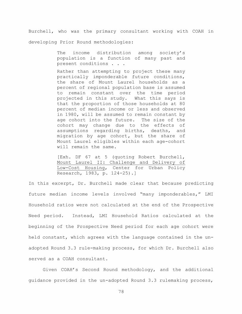
78
Burchell, who was the primary consultant working with COAH in
developing Prior Round methodologies:
The income distribution among society’s population is a function of many past and present conditions . . .
Rather than attempting to project these many practically imponderable future conditions, the share of Mount Laurel households as a percent of regional population base is assumed to remain constant over the time period projected in this study. What this says is that the proportion of those households at 80 percent of median income or less and observed in 1980, will be assumed to remain constant by age cohort into the future. The size of the cohort may change due to the effects of assumptions regarding births, deaths, and migration by age cohort, but the share of Mount Laurel eligibles within each age-cohort will remain the same.
[Exh. DF 67 at 5 (quoting Robert Burchell, Mount Laurel II: Challenge and Delivery of Low-Cost Housing, Center for Urban Policy Research, 1983, p. 124-25).]
In this excerpt, Dr. Burchell made clear that because predicting
future median income levels involved “many imponderables,” LMI
Household ratios were not calculated at the end of the Prospective
Need period. Instead, LMI Household Ratios calculated at the
beginning of the Prospective Need period for each age cohort were
held constant, which agrees with the language contained in the un-
adopted Round 3.3 rule-making process, for which Dr. Burchell also
served as a COAH consultant.
Given COAH’s Second Round methodology, and the additional
guidance provided in the un-adopted Round 3.3 rulemaking process,

79
as well as by COAH’s former Executive Director and Dr. Burchell,
the court concludes that the proper approach here is to calculate
LMI Household Ratios, by age cohort, at the beginning of the
Prospective Need period, then apply those ratios to Total
Households at the beginning and end of the period to determine LMI
Household Growth. The court also concludes that the resulting LMI
Household Growth Rate during the Prospective Need period should be
“about 40 percent”.
(a) Dr. Angelides
Dr. Angelides did apply constant 2015 LMI Household Ratios to
2025 household data, but as discussed previously, he utilized
median incomes derived directly from ACS data instead of using the
COAH income grid. Dr. Angelides’ approach resulted in a negligible
variation in LMI rates for 2015 and 2025 when aggregated to the
State level and an LMI Household Growth Rate of 40.71 percent, as
shown in the following chart:
Dr. Angelides LMI Household Projections 2015 – 2025
2015 2025
Total HHs 3,252,210 3,398,450
LMI HHs 1,298,400 1,357,940
LMI HH Ratio 39.92% 39.96%
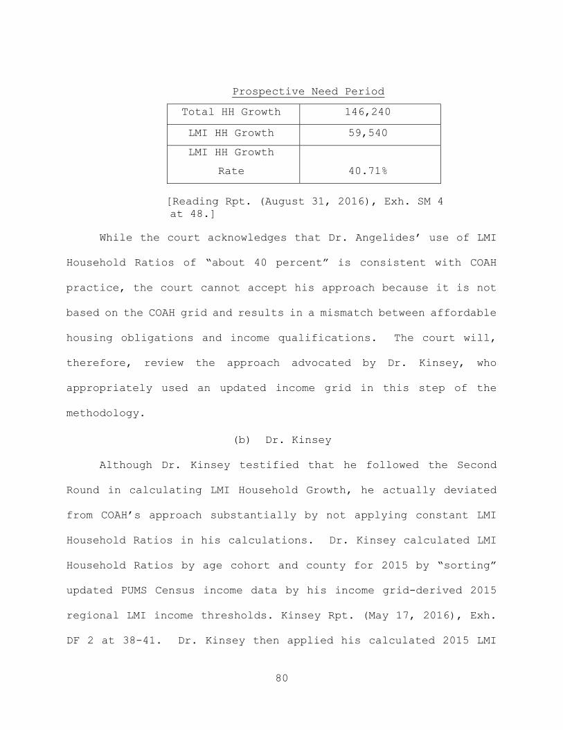
80
Prospective Need Period
Total HH Growth 146,240
LMI HH Growth 59,540
LMI HH Growth
Rate 40.71%
[Reading Rpt. (August 31, 2016), Exh. SM 4 at 48.]
While the court acknowledges that Dr. Angelides’ use of LMI
Household Ratios of “about 40 percent” is consistent with COAH
practice, the court cannot accept his approach because it is not
based on the COAH grid and results in a mismatch between affordable
housing obligations and income qualifications. The court will,
therefore, review the approach advocated by Dr. Kinsey, who
appropriately used an updated income grid in this step of the
methodology.
(b) Dr. Kinsey
Although Dr. Kinsey testified that he followed the Second
Round in calculating LMI Household Growth, he actually deviated
from COAH’s approach substantially by not applying constant LMI
Household Ratios in his calculations. Dr. Kinsey calculated LMI
Household Ratios by age cohort and county for 2015 by “sorting”
updated PUMS Census income data by his income grid-derived 2015
regional LMI income thresholds. Kinsey Rpt. (May 17, 2016), Exh.
DF 2 at 38-41. Dr. Kinsey then applied his calculated 2015 LMI
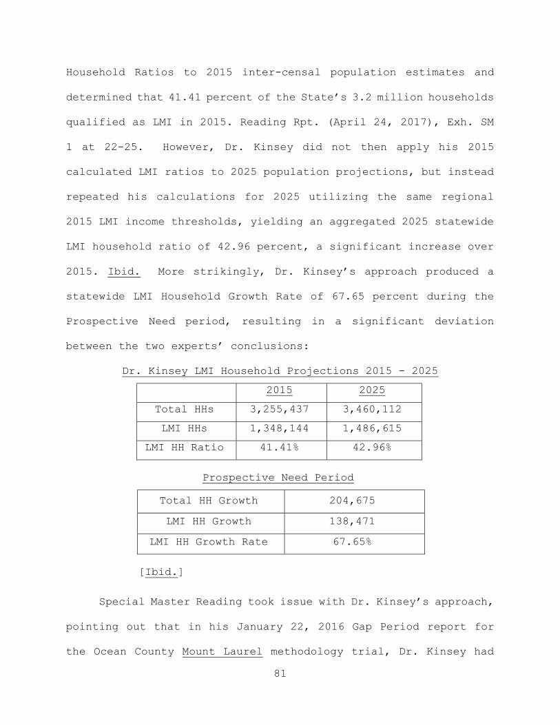
81
Household Ratios to 2015 inter-censal population estimates and
determined that 41.41 percent of the State’s 3.2 million households
qualified as LMI in 2015. Reading Rpt. (April 24, 2017), Exh. SM
1 at 22-25. However, Dr. Kinsey did not then apply his 2015
calculated LMI ratios to 2025 population projections, but instead
repeated his calculations for 2025 utilizing the same regional
2015 LMI income thresholds, yielding an aggregated 2025 statewide
LMI household ratio of 42.96 percent, a significant increase over
2015. Ibid. More strikingly, Dr. Kinsey’s approach produced a
statewide LMI Household Growth Rate of 67.65 percent during the
Prospective Need period, resulting in a significant deviation
between the two experts’ conclusions:
Dr. Kinsey LMI Household Projections 2015 - 2025
2015 2025
Total HHs 3,255,437 3,460,112
LMI HHs 1,348,144 1,486,615
LMI HH Ratio 41.41% 42.96%
Prospective Need Period
Total HH Growth 204,675
LMI HH Growth 138,471
LMI HH Growth Rate 67.65%
[Ibid.]
Special Master Reading took issue with Dr. Kinsey’s approach,
pointing out that in his January 22, 2016 Gap Period report for
the Ocean County Mount Laurel methodology trial, Dr. Kinsey had

82
projected LMI Household Ratios to be stable and essentially
unchanged at about 41.30 percent during the 1999 to 2015 Gap
Period. Reading Rpt. (April 24, 2017), Exh. SM 1 at 26-27 (citing
Exh. P 98 at 19). Mr. Reading concluded that while Dr. Kinsey’s
statewide 2015 LMI Household Ratio of 41.41 percent for these
proceedings appeared to be within reasonable proximity to COAH’s
previously endorsed range, his 2025 ratio of 42.96 percent was an
outlier, which Mr. Reading concluded was caused by Dr. Kinsey’s
inappropriate mixing of data sources. Id. at 22. Moreover, Mr.
Reading concluded that Dr. Kinsey’s significant increase in LMI
proportions between 2015 and 2025 led to the untenable conclusion
that 67.65 percent of total household growth during the Prospective
Need period was in LMI households.
Mr. Reading reiterated that, as in the calculations of
headship rates, it is not the absolute LMI Household Ratios that
have a disproportionate effect on LMI Household Growth, but rather
the changes between those ratios over the Prospective Need period.
As an example, Mr. Reading demonstrated that an increase of two
percent in LMI household ratios over the Prospective Need period
in a state with 3.3 million households would add about 66,000 LMI
households. Mr. Reading further illustrated his point when he
adjusted Dr. Kinsey’s approach by applying constant 2015 LMI
household ratios to Dr. Kinsey’s 2025 Total Households
projections, which yielded a decrease of 26.24 percentage points
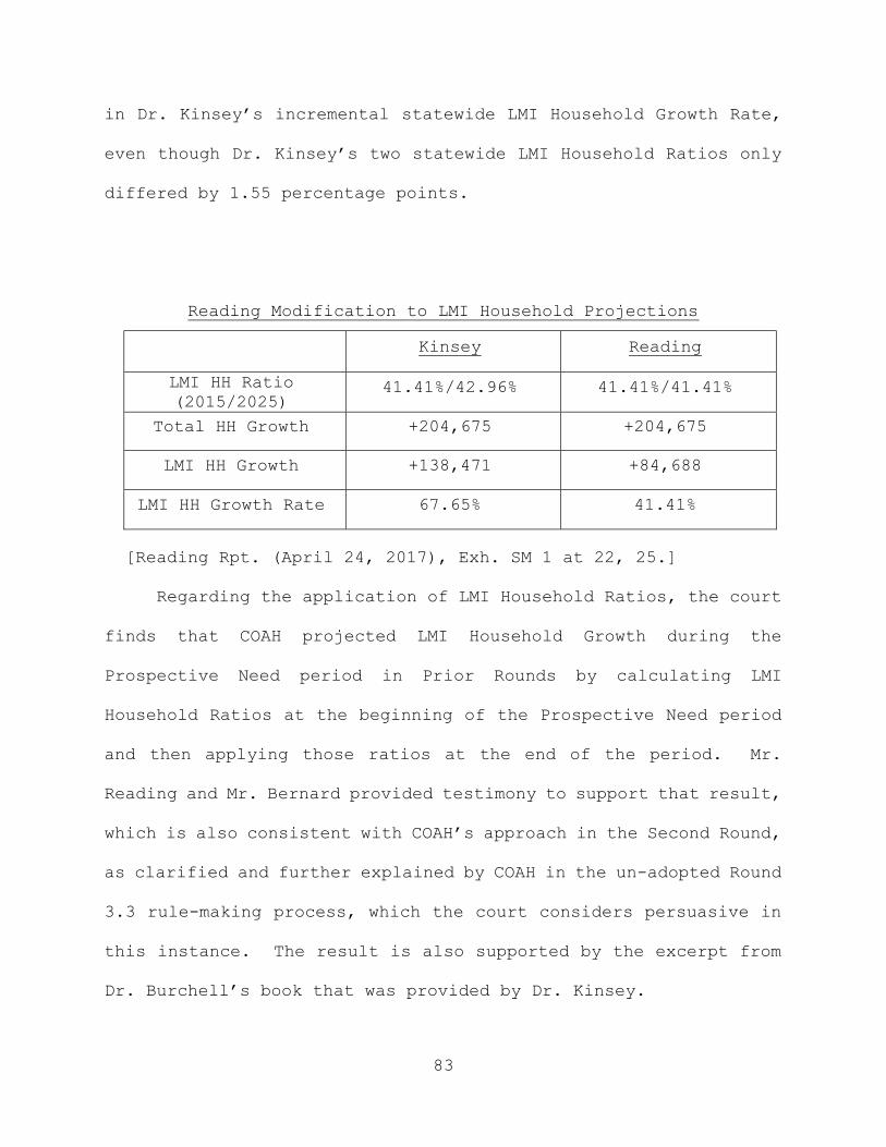
83
in Dr. Kinsey’s incremental statewide LMI Household Growth Rate,
even though Dr. Kinsey’s two statewide LMI Household Ratios only
differed by 1.55 percentage points.
Reading Modification to LMI Household Projections
Kinsey Reading
LMI HH Ratio (2015/2025)
41.41%/42.96% 41.41%/41.41%
Total HH Growth +204,675 +204,675
LMI HH Growth +138,471 +84,688
LMI HH Growth Rate 67.65% 41.41%
[Reading Rpt. (April 24, 2017), Exh. SM 1 at 22, 25.]
Regarding the application of LMI Household Ratios, the court
finds that COAH projected LMI Household Growth during the
Prospective Need period in Prior Rounds by calculating LMI
Household Ratios at the beginning of the Prospective Need period
and then applying those ratios at the end of the period. Mr.
Reading and Mr. Bernard provided testimony to support that result,
which is also consistent with COAH’s approach in the Second Round,
as clarified and further explained by COAH in the un-adopted Round
3.3 rule-making process, which the court considers persuasive in
this instance. The result is also supported by the excerpt from
Dr. Burchell’s book that was provided by Dr. Kinsey.
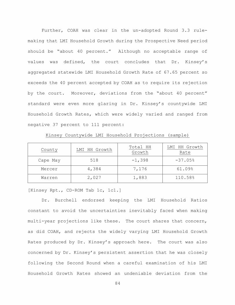
84
Further, COAH was clear in the un-adopted Round 3.3 rule-
making that LMI Household Growth during the Prospective Need period
should be “about 40 percent.” Although no acceptable range of
values was defined, the court concludes that Dr. Kinsey’s
aggregated statewide LMI Household Growth Rate of 67.65 percent so
exceeds the 40 percent accepted by COAH as to require its rejection
by the court. Moreover, deviations from the “about 40 percent”
standard were even more glaring in Dr. Kinsey’s countywide LMI
Household Growth Rates, which were widely varied and ranged from
negative 37 percent to 111 percent:
Kinsey Countywide LMI Household Projections (sample)
County LMI HH Growth Total HH Growth
LMI HH Growth Rate
Cape May 518 -1,398 -37.05%
Mercer 4,384 7,176 61.09%
Warren 2,027 1,883 110.58%
[Kinsey Rpt., CD-ROM Tab 1c, 1c1.]
Dr. Burchell endorsed keeping the LMI Household Ratios
constant to avoid the uncertainties inevitably faced when making
multi-year projections like these. The court shares that concern,
as did COAH, and rejects the widely varying LMI Household Growth
Rates produced by Dr. Kinsey’s approach here. The court was also
concerned by Dr. Kinsey’s persistent assertion that he was closely
following the Second Round when a careful examination of his LMI
Household Growth Rates showed an undeniable deviation from the

85
COAH approach. Moreover, Dr. Kinsey himself used a constant
household growth ratio in at least one report that he produced in
the course of the Third Round judicial proceedings.
In this step of the methodology, then, the court finds that
neither expert’s approach is satisfactory, with both deviating
from COAH’s Prior Round methodology in unacceptable ways. Dr.
Angelides’ approach applied constant LMI Household Ratios, but
disregarded COAH’s explicit policy decision to utilize the COAH
income grid, while Dr. Kinsey utilized an updated COAH-inspired
income grid, but failed to apply constant LMI Household Ratios as
COAH did in the Prior Rounds. Notably, Mr. Reading’s modification
of Dr. Kinsey’s approach utilized both an updated income grid and
constant LMI Household Ratios. Therefore, the court will adopt
Mr. Reading’s modification of Dr. Kinsey’s approach, utilizing
constant 2015 LMI Household Ratios, calculated using Dr. Kinsey’s
updated COAH income grid as endorsed by the court in the previous
step. Note, however, that some of the numbers contained in the
following chart differ from those on page 83 due to the use of
updated population figures and the trended headship rate
adjustment that the court directed Mr. Reading to use in making
the calculations required by this decision. As a result, the
following chart shows the aggregated New Jersey estimated LMI
Household Growth incorporated into the court’s fair share
methodology:
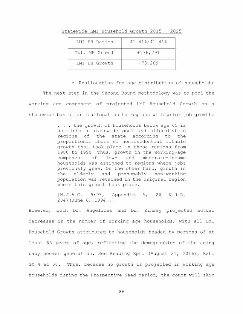
86
Statewide LMI Household Growth 2015 – 2025
LMI HH Ratios 41.41%/41.41%
Tot. HH Growth +176,791
LMI HH Growth +73,209
e. Reallocation for age distribution of households
The next step in the Second Round methodology was to pool the
working age component of projected LMI Household Growth on a
statewide basis for reallocation to regions with prior job growth:
. . . the growth of households below age 65 is put into a statewide pool and allocated to regions of the state according to the proportional share of nonresidential ratable growth that took place in these regions from 1980 to 1990. Thus, growth in the working-age component of low- and moderate-income households was assigned to regions where jobs previously grew. On the other hand, growth in the elderly and presumably non-working population was retained in the original region where this growth took place.
[N.J.A.C. 5:93, Appendix A, 26 N.J.R. 2347(June 6, 1994).]
However, both Dr. Angelides and Dr. Kinsey projected actual
decreases in the number of working age households, with all LMI
Household Growth attributed to households headed by persons of at
least 65 years of age, reflecting the demographics of the aging
baby boomer generation. See Reading Rpt. (August 31, 2016), Exh.
SM 4 at 50. Thus, because no growth is projected in working age
households during the Prospective Need period, the court will skip

87
this step in the methodology for the Third Round from 2015-2025,
as did both experts.
f. Account for older LMI households with significant housing assets (Angelides proposal)
Dr. Angelides included a “significant housing assets” test in
his Prospective Need methodology to remove from LMI household
projections those LMI households that were LMI with respect to
annual household income, but that possess significant housing
assets. Dr. Angelides noted that the UHAC regulations contain a
real estate asset test that would disqualify otherwise income-
eligible LMI households from qualifying for affordable housing.
Angelides Rpt. (May 16, 2016), Exh. P 2 at 52 (citing N.J.A.C.
5:80-26.16(b)3). Dr. Angelides also noted that each iteration of
COAH’s Third Round methodology included an asset test. Ibid. He
applied his test comparing the sum of eligible assets as reported
in the 2014 one-year PUMS to the 2014 regional asset limits
published by COAH, calculating the proportion of disqualified LMI
households by region and household size. Dr. Angelides’ test
yielded an aggregated statewide proportion of 8.8 percent of the
LMI Household Growth between 2015 and 2025. Application of this
proportion resulted in a decrease of 5,400 LMI households
statewide. Reading Rpt. (August 31, 2016), Exh. SW 4 at 50.
Mr. Bernard testified that COAH had considered excluding LMI
households with assets, along with other potential changes, in
88
both the First and Second Rounds, but declined to do so. In
addition, the defendants pointed out that although COAH did include
an asset test in the various iterations of the Third Round rules,
the impact of using the test -- which would have decreased fair
share obligations -- was offset by other changes that would have
increased fair share obligations. Special Master Reading noted
that since all projected growth in New Jersey is anticipated to be
in senior citizen households, an asset test made sense because
many senior citizens own their own homes, often mortgage-free, and
are thus not in need of affordable housing. In the final analysis,
however, Mr. Reading recommended against adopting this test
because it had not been included by COAH in the First or Second
Rounds and constituted an important policy decision that he
concluded should be vetted by an agency reviewing a comprehensive
revision of COAH rules before adoption.
The court acknowledges that COAH declined to include an asset
test in the Prior Rounds, but then did so in all three iterations
of its Third Round rules. However, in each of the three
iterations, COAH linked the reduction of affordable housing
obligations that would result from an asset test with an offset
from a new calculation that would likely increase need, such as
including individuals living in certain group quarters. COAH
stated in Round 3.2 that:

89
low- and moderate-income owners with significant assets – those who have paid off their mortgages and spend less than 38 percent of their income on other housing costs – are removed from [affordable housing obligations], and low- and moderate-income residents of noninstitutional group quarters are added to [affordable housing obligations], to reach a Total Projected Need . . .
[N.J.A.C. 5:97 (“Round 3.2”), App. A, 89.]
And in Round 3.3. COAH similarly asserted that:
While owners with significant assets reduce the overall need, demand from low- and moderate-income households in group quarters increases the overall need. The 2000 and 2010 Censuses specify the populations in [noninstitutionalized] group quarters… A portion of residents living in “other” noninstitutional group quarters are included in this methodology.
[46 N.J.R. (“Round 3.3”), 984; see also N.J.A.C. 5:94 (“Round 3.1”), 65, 79.]
While the asset test constitutes a reasonable revision to
Prior Round methodology, it is the kind of policy decision that
should be fully vetted by an administrative agency in the context
of rulemaking. Here, COAH did consider and adopt such an asset
test as part of its Third Round rules, and did provide sufficient
detail to allow Dr. Angelides to replicate the test for the current
Prospective Need period. However, the addition of the asset test
was never specifically approved by the Appellate Division and, as
previously noted, COAH included the asset test along with a
companion offset, which Dr. Angelides did not include in his
methodology, and which has not been incorporated into the model

90
endorsed by this court. Consequently, the court will include
neither an asset test nor its companion off-set step in its fair
share methodology, leaving the decision to incorporate these
policy changes for the future when an agency better equipped to
review and balance new policy initiatives becomes functional. This
result is consistent with the Supreme Court’s admonition to the
trial courts to concentrate on accepted methodologies and to avoid
unnecessary policy determinations better left to administrative
rulemaking. Mount Laurel IV, 221 N.J. at 29-30. Therefore, the
court will not adopt Dr. Angelides’ proposed asset test.
g. Aggregate Regional Prospective Need
The next step is to aggregate LMI household growth during the
Prospective Need period to yield gross Prospective Need by region,
which will be subsequently allocated to the municipalities and
adjusted for secondary sources. Both experts followed COAH
methodology established in the Prior Rounds in this step, reaching
different results because of their divergent approaches in the
earlier steps. Included here are the statewide and Region 4
values, calculated pursuant to the methodology steps endorsed in
this decision:
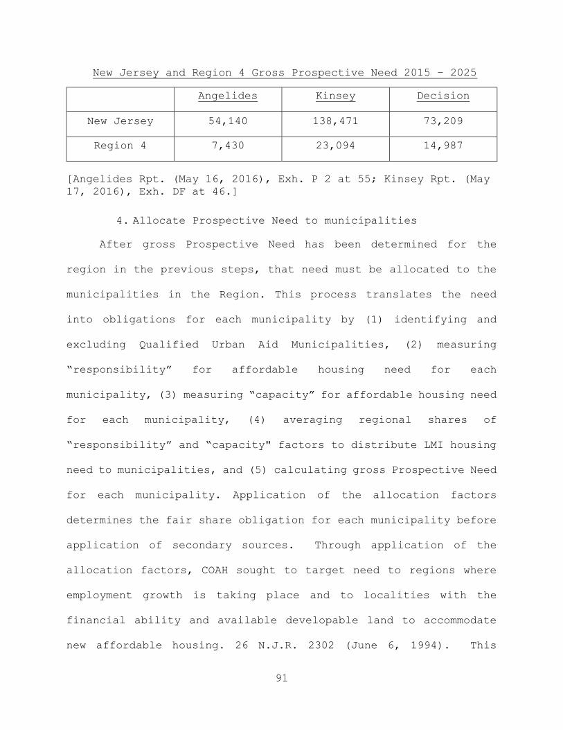
91
New Jersey and Region 4 Gross Prospective Need 2015 – 2025
Angelides Kinsey Decision
New Jersey 54,140 138,471 73,209
Region 4 7,430 23,094 14,987
[Angelides Rpt. (May 16, 2016), Exh. P 2 at 55; Kinsey Rpt. (May 17, 2016), Exh. DF at 46.]
4. Allocate Prospective Need to municipalities
After gross Prospective Need has been determined for the
region in the previous steps, that need must be allocated to the
municipalities in the Region. This process translates the need
into obligations for each municipality by (1) identifying and
excluding Qualified Urban Aid Municipalities, (2) measuring
“responsibility” for affordable housing need for each
municipality, (3) measuring “capacity” for affordable housing need
for each municipality, (4) averaging regional shares of
“responsibility” and “capacity" factors to distribute LMI housing
need to municipalities, and (5) calculating gross Prospective Need
for each municipality. Application of the allocation factors
determines the fair share obligation for each municipality before
application of secondary sources. Through application of the
allocation factors, COAH sought to target need to regions where
employment growth is taking place and to localities with the
financial ability and available developable land to accommodate
new affordable housing. 26 N.J.R. 2302 (June 6, 1994). This
92
allocation process once again requires the court to select among
various datasets and divergent recommendations from the experts.
Notably, however, none of these factors alter total need, but
govern how the need is allocated to municipalities.
a. Identify and Exclude Qualified Urban Aid Municipalities
COAH Prior Round methodologies excluded a category of
municipalities with higher-than-average proportions of LMI
families living in fiscally/economically distressed areas from
additional LMI housing requirements, known as Qualified Urban Aid
Municipalities (“QUAMs”), as designated by the DCA. N.J.A.C. 5:93,
Appendix A, 26 N.J.R. 2346, attachment at 2352 (June 6, 1994). To
be designated as a QUAM, a municipality must satisfy at least one
of three criteria: (1) a level of existing LMI housing deficiency
in excess of the average LMI deficiency in its region, (2) a
population density in excess of 10,000 persons per square mile, or
(3) a population density between 6,000 and 10,000 persons per
square mile and less than 5 percent vacant (non-farm) land measured
by the average of the percentage of parcels and valuation in the
municipality. Ibid. See also 46 N.J.R. 952 (June 2, 2014).
Dr. Angelides excluded 42 of the 58 QUAMs, while Dr. Kinsey
exempted 48. Both experts identified the same four Region 4
municipalities for exemption: Trenton, Asbury Park, Long Branch,

93
and Lakewood. As a result, no further discussion is warranted on
this point for Mercer County.
The formula for the allocation of regional Prospective Need
to non-exempted municipalities in the Prior Rounds relied upon a
mix of what COAH characterized as “responsibility” and “capacity”
factors, which reflect the economic and land use concerns
referenced above. These factors address whether a municipality can
physically accommodate growth in terms of available developable
land, and also evaluate the financial ability of towns to address
affordable housing need. Once calculated for each municipality,
each factor is totaled for the region, and each municipality is
assigned a percentage of that regional total. The Second Round
recognized three allocation factors -- one “responsibility” factor
and two “capacity” factors -- which were averaged for each
municipality. Then that percentage was applied to the regional
Prospective Need to determine each municipality’s share of
regional need.
b. Calculate Responsibility Factor for Each Municipality as a Share of its Region
Responsibility factors represent “measures of responsibility,
i.e., the labor force either existing in the community or drawn to
the municipality in the future . . . needing housing.” N.J.A.C.
5:93, Appendix A, 26 N.J.R. 2346 (June 6, 1994). In essence, COAH
sought to apportion affordable housing obligations to
94
municipalities based in part on employment and anticipated
employment growth that generated the need to house workers. While
once again this concept appears to be straightforward, the absence
of reliable data proved problematic for COAH, and remains
problematic for this court.
COAH measured employment-generating activities directly in
the First Round, using Department of Labor employment statistics
reported on a municipal basis. This data source proved
troublesome, however, due to what has been identified as the “zip
code problem.” It turned out that the business mailing addresses
used by the Department of Labor did not always reflect the actual
municipality in which the business is located. Ibid. An example
of this phenomenon is that parts of South Brunswick and Montgomery
Townships have a Princeton zip code, but are located in Middlesex
and Somerset Counties, respectively, and not in Mercer County where
Princeton is located. So employment data collected by mailing
address was inaccurate for a number of municipalities. In
addition, employers often reported total labor statistics from
their headquarters, combining employees working at different
locations, including at facilities in other municipalities. This
phenomenon became known as the “headquarters problem,” a reporting
glitch that also inaccurately skewed some municipal employment
data. As a result of these problems, a number of municipalities
challenged the affordable housing obligations COAH allocated to
95
them in the First Round. After confirming the assertions of some
municipalities that the employment data used in the First Round
had improperly been inflated, leading to higher affordable housing
obligations than were warranted, COAH reduced the obligations of
those towns. As a result, many units included in municipal need
in the First Round were lost and not replaced.
Not wanting to repeat this problem, which had diluted
statewide affordable housing obligations, COAH sought a remedy in
the Second Round. It consequently replaced the faulty direct
measures of employment and employment growth with a single “change
in equalized non-residential property valuation,” known as the
“non-residential valuation growth” factor, concluding that,
“[r]eal property valuation . . . has been found to be an excellent
surrogate for the intensity of use or number of employees in the
structure.” 26 N.J.R. 2346 (June 6, 1994). COAH relied on data
collected and reported annually by the Division of Local Government
Services in the NJDCA. As noted by COAH, “Equalized valuation
through the application of assessment-to-sales or equalization
ratio is used to standardize for the differing levels of assessment
relative to true or market values that exist in an individual
community.” Ibid. Dr. Kinsey incorporated the non-residential
valuation growth factor into his methodology, essentially
following COAH’s approach in the Second Round, but modifying it to

96
include growth from 1990 through 2015 because COAH had used 1990
data as the endpoint in the Second Round.
Dr. Angelides disagreed with this approach, concluding that
the non-residential valuation surrogate was problematic due to the
lack of direct correlation between valuation and employment
density, the susceptibility of the surrogate to non-employment
forces (i.e. the real estate market), and the arbitrary manner in
which revaluations and reporting are performed. Dr. Angelides
concluded that these issues rendered the validity of the valuation
surrogate suspect, despite COAH’s endorsement of the approach in
the Second Round. As a result, Dr. Angelides replaced the non-
residential valuation growth factor in favor of municipal
employment data drawn from a 2013 dataset known as the Longitudinal
Employer-Household Dynamics Origin-Destination Employment
Statistics (“LODES”), a product developed by the United States
Census Bureau, and apparently used primarily for transportation
planning. According to Dr. Angelides, LODES data, which was not
available to COAH during the Second Round, provided direct
employment data on a municipal level and would accomplish the
direct measure that COAH had utilized in the First Round, but
allegedly without the zip code or headquarters problems. Notably,
however, Dr. Angelides admitted that he had simply incorporated
LODES data for the State and Mercer County into his model without
verifying its accuracy.
97
Dr. Kinsey not only urged the court to follow the Second Round
procedures as more consistent with COAH practice, but also
challenged the reliability of the LODES data used by Dr. Angelides
because of inaccuracies Dr. Kinsey claimed are caused by the
statistical techniques employed to protect the confidentiality of
aspects of the data. While the court did not fully understand
what Dr. Kinsey characterized as “noise” that was introduced into
the data collection process to protect employer confidentiality,
but which he claimed had the effect of introducing inaccuracies
into the data, Dr. Kinsey presented compelling evidence of specific
instances in Mercer County where LODES data appeared to be
erroneous. For example, from 2012 to 2014, LODES employment data
in Hopewell Township in the health care sector remained static
although it is well known that Capital Health opened a large new
hospital there during that period with over 1500 employees. Ewing
Township, however, which adjoins Hopewell, showed an increase of
1800 health care jobs in the same time frame with no obvious
justification for that increase. LODES data also showed an
inexplicable drop in Trenton employment from 2013 to 2014 of over
25,000 jobs. LODES data for Ewing over the past fifteen years
also showed significant swings of between 5,000 and 17,000 jobs in
several years with no apparent explanation.
Mr. Bernard confirmed COAH’s experience as summarized above,
noting that the Second Round had solved the zip code and
98
headquarters problems. Indeed, he testified that no town objected
to the application of the responsibility factor based on its non-
residential ratables, preventing the dilution of need that had
occurred in the First Round. While he admitted that non-
residential ratables were an imperfect surrogate for jobs, he
asserted that such ratables showed the fiscal capacity of a town
to absorb affordable housing, and operated as a fair and effective
surrogate on this basis. He expressed concern that if the court
adopted the use of LODES data as advocated by Dr. Angelides,
municipalities could petition the court for corrections based on
inaccuracies in the data, propelling the court into the same
dilemma faced by COAH in the First Round.
Mr. Reading candidly admitted that neither approach urged by
the experts was satisfactory. While he identified what he termed
a “disconnect” between job growth and ratable growth, he was
troubled by the clear inaccuracies in the LODES data for Mercer
County. He agreed with Mr. Bernard, however, that non-residential
ratables in a town are associated with a responsibility to provide
housing for the workers employed there. Although Mr. Reading liked
the idea of a direct measure of employment and thought LODES data
showed promise, he could not recommend its use because it has never
been validated for New Jersey. He somewhat reluctantly endorsed
Dr. Kinsey’s approach as being generally consistent with COAH’s
procedure in the Second Round.
99
The court once again is faced with a choice between two
imperfect and imprecise alternatives. Notably, neither set of
statistics was developed for the purpose for which it is being
introduced into the model —- allocating affordable housing to
municipalities based on employment. Given the clear inaccuracies
in the LODES data for Mercer County, however, the court concurs
with Mr. Reading’s assessment that the Second Round valuation
surrogate should continue to be used in this step, as advocated by
Dr. Kinsey and Mr. Bernard. COAH made a policy choice in the
Second Round to replace the direct measures of employment it had
used to assess municipal responsibility factors in the First Round
with a valuation surrogate, as the solution to specific problems
it identified. That surrogate was used without apparent objection
in the Second Round, with the advantage of directing need to
municipalities with non-residential ratable growth. Any
reevaluation of COAH’s Second Round data choice to measure this
responsibility factor involves policy decisions best left to an
administrative agency that can fully analyze the matter and explore
alternatives in a systematic way. While the court would have
considered changing datasets if the Second Round valuation
surrogate was shown to be clearly defective and a demonstrably
superior alternative was available, neither circumstance was
supported by the record here. The only thing that is clear is
that neither approach is without shortcomings. As a result, the

100
court adopts Dr. Kinsey’s methodology that utilizes the Second
Round single non-residential valuation growth factor and will
leave the possible use of LODES data, or another alternative, to
a reconstituted COAH in the future.
c. Calculate Capacity Factors for Each Municipality as a Share of its Region
Municipal “capacity” factors represent “measures of capacity,
i.e., the physical (land) and fiscal (income) capacity to absorb
and provide for [affordable] housing.” N.J.A.C. 5:93, Appendix A,
26 N.J.R. 2346 (June 6, 1994). In the Second Round, income
capacity was determined by measures of income differences between
the municipality and the region, while “physical” capacity was
based on an analysis of the proportion of the region’s undeveloped
land located within each municipality that could accommodate
development.
i. Income Capacity Factor
COAH changed the income capacity factor calculation for the
Second Round because the straightforward calculation of a
municipality’s share of its regional aggregate income in the First
Round “tended to give large middle-class municipalities an
overabundance of low- and moderate-income housing need because
they had a lot of households with reasonably healthy incomes.”
N.J.A.C. 5:93, Appendix A, 26 N.J.R. 2346 (June 6, 1994). In its
place, the Second Round calculated the average of two measures:
101
a. Municipal share of the regional sum of the differences between median 1993 municipal household income and an income floor ($100 below the lowest average household income in the region), and b. Municipal share of the regional sum of the differences between median 1993 municipal household incomes and an income floor ($100 below the lowest 1993 median household income in the region) weighted by the number of the households in the municipality. [N.J.A.C. 5:93, Appendix A, 26 N.J.R. 2346 (June 6, 1994).]
By using household income differences in municipalities
rather than income, as was used in the First Round, as well as
weighting, COAH sought to “dampen the extremes of the straight-
difference income allocation index,” utilized in the First Round.
In commenting on this change, COAH noted that, “It is believed
that the procedure achieves both equity and more incisive income
targeting.” Ibid.
Dr. Angelides adopted the Second Round methodology, but with
modifications to correct what he saw as mathematical errors
regarding both the mixing of median and mean in the first
calculation, and a statistically inappropriate use of medians in
the second. Dr. Kinsey followed the Second Round methodology,
utilizing ACS 2010-2014 data to establish municipal median and
regional “floor” income levels. Mr. Reading found that the
differences between the two methodologies had a minimal effect on
the allocation of need, and recommended Dr. Kinsey’s methodology

102
as adhering more closely to the Second Round. Given the minimal
impact on the allocation of municipal affordable housing need, Mr.
Reading’s endorsement of Dr. Kinsey’s approach, and its
consistency with the Second Round, the court adopts Dr. Kinsey’s
approach for calculation of the income capacity factor.
ii. Land Capacity Factor
The land capacity factor considers undeveloped land in the
community that can accommodate development. The complexity
involved in this determination derives in part from the fact that
not all vacant land is developable, and from the shortcomings of
the datasets used by the experts. The Second Round estimated the
undeveloped land in municipalities utilizing land satellite
imagery (LANDSAT), which was compiled for COAH by Rutgers
University. N.J.A.C. 5:93, Appendix A, 26 N.J.R. 2346 (June 6,
1994). The undeveloped land was then weighted in accordance with
the “Planning Areas” in the State Development and Redevelopment
Plan. Ibid. COAH cross-checked the undeveloped land by
municipality with data from The New Jersey Department of Treasury,
Division of Taxation, finding that the LANDSAT data was “an
excellent and comprehensive source of land-use information.” COAH
noted that the data contained information for every municipality
in the State so that its strengths and weaknesses applied equally
to most municipalities, making LANDSAT “a very comprehensive and
important source of undeveloped land information especially good
103
for relative comparisons.” Ibid. Mr. Bernard noted that COAH in
the Second Round was looking for a uniform and reliable source of
information, and was satisfied that LANDSAT satisfied these
concerns.
Dr. Kinsey followed COAH’s Second Round methodology, with
certain revisions to incorporate the updated 2001 State
Development and Redevelopment Plan, the revised (2004) Meadowlands
Master Plan, and the land classifications in the 2008 Highlands
Regional Master Plan. Reading Rpt. (August 31, 2016), Exh. SM 4 at
57. Dr. Kinsey also utilized updated “land use/land cover data”
from the New Jersey Department of Environmental Protection’s
(NJDEP) 2007 land use mapping product, which was released in 2010
and was based on work performed through a joint Rowan University-
Rutgers University initiative. The major shortcoming of this
procedure was the age of the data used to apply this factor in the
Third Round, which started in 2015. Mr. Bernard did note, however,
that since the data was collected before the start of the recession
and New Jersey’s recovery had been slow, limited development in
recent years made the age of the imagery less problematic than it
would have been had the recent past seen significant development.
Dr. Angelides likewise followed the Second Round by
considering the allocation of municipal shares of regional
affordable housing need as the ratio of undeveloped land in each
municipality as a percentage of that in the region. However, Dr.
104
Angelides expressed skepticism as to whether vacant, undeveloped
land could act as an accurate measure of capacity as it does not
take into account repurposing of existing non-residential
buildings or demolition of underutilized structures, which he
concluded biases development toward suburban green field
locations.
Dr. Angelides also expressed concern that the 2007 NJDEP
imagery was nine years old at the time Dr. Kinsey prepared his
model, that it was of poor resolution, and that the Rutgers/Rowan
analysis was not reproducible or verifiable. Thus, Dr. Angelides
deviated from the Second Round by utilizing parcel-level tax
assessment data from the New Jersey Property Tax System instead of
land imagery to determine potentially developable parcels in each
municipality. Dr. Angelides then accounted for environmental
restrictions and state planning designations by overlaying the tax
assessment data with visual displays of geographic data from the
NJDEP Bureau of Geographic Information Systems. Dr. Angelides
then applied a weighting system based upon planning designations
from the Second Round to undeveloped acreage that reflected its
conduciveness to development. The shortcomings of this approach
were that the data contained inconsistencies and had been shown to
be incomplete, with up to 15 percent of local tax records lacking
the necessary data to establish the existence of vacant and
developable land. Dr. Kinsey pointed to a glaring error in West

105
Windsor, where the data used by Dr. Angelides showed that a
property of over 90 acres was not considered developable because
it had a small improvement on the large parcel. That property is
owned by a developer that intervened in West Windsor’s declaratory
judgment action seeking to build affordable housing on that
property.
Mr. Reading concluded that, although Dr. Angelides’ reliance
on municipal block and lot classifications of land use instead of
aerial surveys could offer a more accurate and up-to-date method,
his approach depended upon classifications performed by individual
municipal assessors, and therefore lacked statewide uniformity.
Mr. Reading further concluded that any inaccuracies in the land
imagery data due to recent development could be addressed by
adjustments made in each town’s compliance process. Mr. Reading
once again recommended Dr. Kinsey’s methodology as it conformed
more closely to COAH’s Second Round methodology.
The court concurs with Mr. Reading’s assessment that, given
yet another choice between two imperfect alternatives, following
the Second Round approach is the best option, especially since
that approach relies on data derived from a single consistent
source that can be corrected during the compliance process.
Moreover, the court once again is hesitant to endorse a new
approach never validated or tested in any way by COAH. The court
106
therefore adopts Dr. Kinsey’s method for calculating the land
capacity factor.
d. Average Regional Shares of “responsibility” and “capacity" Factors and Allocate Gross Prospective Need to Each Municipality
Once the allocation factors are determined, the next step is
to calculate the average allocation factor for each municipality.
In the Second Round, COAH concluded that, “[a]ll factors operate
individually, are equally weighted, and involve all municipalities
in the region except Urban Aid municipalities,” with all
allocations derived from those factors “reflect[ing] the fraction
representing the community's share of the regional total.” N.J.A.C
5:93, Appendix A, 26 N.J.R. 2346 (June 6, 1994). Drs. Angelides
and Kinsey both aggregated each of the factors they calculated by
region and determined each municipality’s share for each factor.
They then averaged the shares of each factor for each municipality,
yielding municipal proportional shares of regional Prospective
Need. Since the court adopted Dr. Kinsey’s three “responsibility”
and “capacity” factors, gross Prospective Need will be allocated
to each municipality following COAH’s Second Round methodology,
based on the average share of Dr. Kinsey’s three factors. The
resulting municipal gross Prospective Need, calculated pursuant to
this decision, is reflected in the following chart:
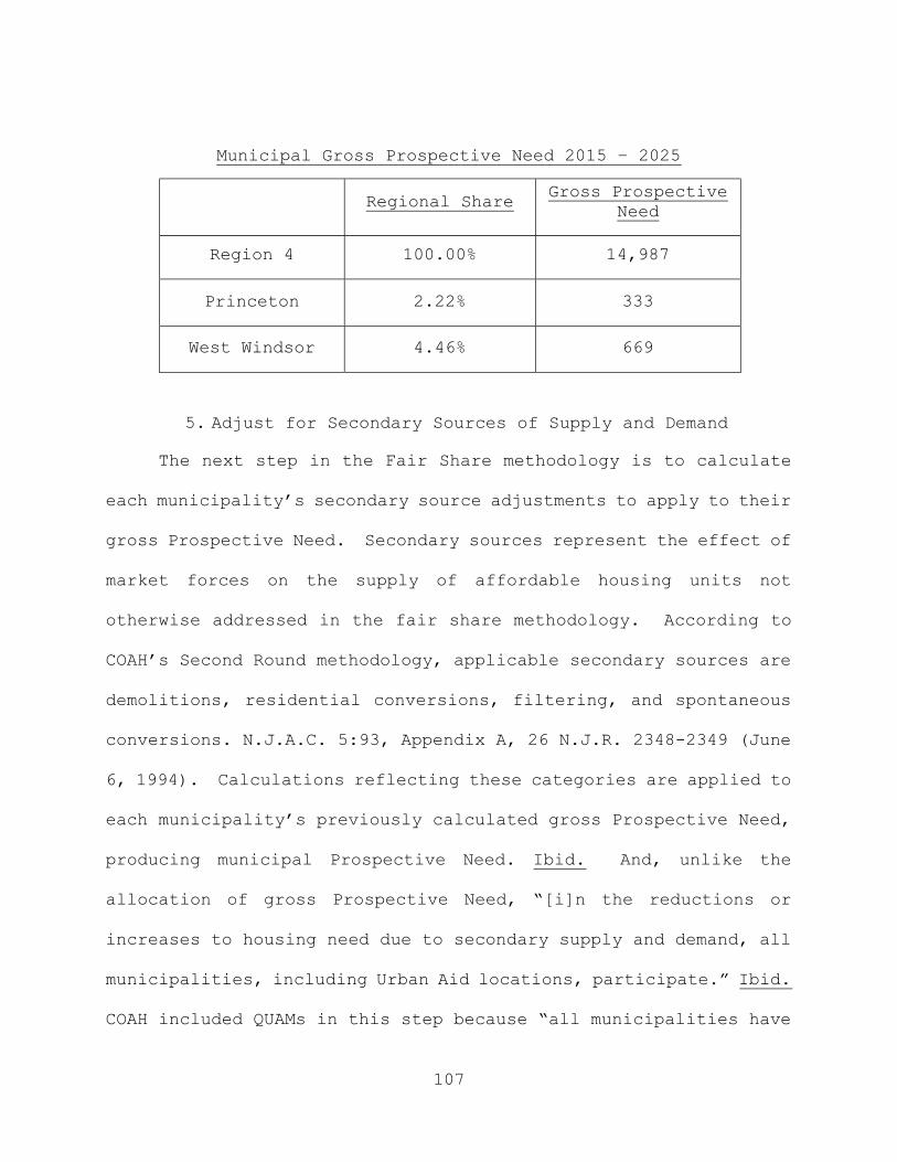
107
Municipal Gross Prospective Need 2015 – 2025
Regional Share Gross Prospective
Need
Region 4 100.00% 14,987
Princeton 2.22% 333
West Windsor 4.46% 669
5. Adjust for Secondary Sources of Supply and Demand
The next step in the Fair Share methodology is to calculate
each municipality’s secondary source adjustments to apply to their
gross Prospective Need. Secondary sources represent the effect of
market forces on the supply of affordable housing units not
otherwise addressed in the fair share methodology. According to
COAH’s Second Round methodology, applicable secondary sources are
demolitions, residential conversions, filtering, and spontaneous
conversions. N.J.A.C. 5:93, Appendix A, 26 N.J.R. 2348-2349 (June
6, 1994). Calculations reflecting these categories are applied to
each municipality’s previously calculated gross Prospective Need,
producing municipal Prospective Need. Ibid. And, unlike the
allocation of gross Prospective Need, “[i]n the reductions or
increases to housing need due to secondary supply and demand, all
municipalities, including Urban Aid locations, participate.” Ibid.
COAH included QUAMs in this step because “all municipalities have
108
some type of housing need, and reductions apply to housing need no
matter how the need is generated.” Ibid.
Although COAH also included spontaneous conversions in its
adopted Round 3.1 rules, they were omitted in Round 3.2 and Round
3.3, and both Drs. Angelides and Kinsey adopted this approach.
Dr. Angelides, however, added a step not included in the Prior
Rounds by reallocating surplus affordable housing credits from
individual municipalities back to the region to offset the
remaining need of other municipalities. As a result, the court
will consider the following secondary source adjustment steps: (1)
demolitions; (2) residential conversions; (3) filtering; (4)
reallocation of secondary source adjustments (Angelides proposal);
and (5) calculation of Prospective Need by Municipality.
a. Demolitions
“Demolitions are a secondary source of housing demand . . .
created by households requiring housing because units are lost
from stock.” N.J.A.C. 5:93, Appendix A, 26 N.J.R. 2348 (June 6,
1994). This “selective pruning” of residential housing units
occurs for a variety of reasons, such as damage from natural
causes, deterioration, redevelopment, or abandonment. “In strong
markets, demolitions are low; in weaker markets, they are
proportionally higher.” Ibid. In both situations, when housing
units affordable to LMI households are lost, their demolition
109
decreases the supply of affordable housing, thus increasing
affordable housing need.
In the Second Round, COAH calculated an estimate of total
demolitions in the six-year Prospective Need period for each
municipality by averaging reported demolitions for the three most
recent years for which municipal demolition data was available,
and then multiplying by six. N.J.A.C. 5:93-2.9. In determining
the LMI share of total municipal demolitions, COAH “recognize[d]
that demolitions take place at a much higher rate in the low- and
moderate-income housing sector than for all housing locally,”
N.J.A.C. 5:93, Appendix A, 26 N.J.R. 2348-2349 (June 6, 1994),
further noting that:
Total demolitions are thus tallied by individual community and the share affecting low- and moderate-income housing is estimated by a multiple of the subregional low- and moderate-income housing deficiency percentage.
[Ibid.]
To calculate the “multiple” in accordance with the Second Round,
and thus determine the LMI share of total municipal demolitions,
COAH provided that:
Demolitions are adjusted for each municipality to the share of all demolitions that affect the low- and moderate-income housing sector by 120 percent of the subregional share of low- and moderate-income housing. This percentage
110
share of all demolitions that affects low- and moderate-income families is capped at 95 percent.
[Ibid.]
Dr. Kinsey utilized NJDCA demolition data from 1999 through
2015 as the basis to estimate total municipal demolitions during
the Prospective Need period, but adjusted the data for the effects
of Hurricane Sandy. Dr. Kinsey accounted for the unusually high
number of storm-related demolitions by applying adjustments for
four Hurricane Sandy-impacted counties, based on the ratio of pre-
and post-Sandy demolitions. Then, Dr. Kinsey calculated municipal
LMI demolitions using each municipality’s share of the county’s
LMI households. While Dr. Kinsey intended to include COAH’s Second
Round multiplier in his calculations, he expressed confusion
during cross-examination as to whether he had actually
incorporated the multiplier into his spreadsheets, suggesting that
any omission on his part had been inadvertent. He also used county
rather than regional incomes in preparing his calculations. Dr.
Kinsey’s resulting estimate of LMI demolitions in each
municipality was aggregated to yield 19,262 projected statewide
demolitions for the Prospective Need period of 2015-2025. Notably,
Dr. Kinsey seemed uncharacteristically unconcerned about any
possible deviations in his calculations from COAH’s approach to
demolitions, and made no effort to clarify the procedure he
actually followed. Perhaps his attitude was prompted by the small
111
variation in demolitions between his figures and those of Dr.
Angelides, which difference Mr. Reading identified as less than 5
percent.
Dr. Angelides also used NJDCA data in his methodology and
adjusted for Hurricane Sandy, but deviated from Second Round
methodology by not applying COAH’s multiplier. Dr. Angelides
calculated average annual total demolitions by municipality from
2000 to 2014 using NJDCA data, but excluding 2012 and 2013
statistics to account for the high number of Hurricane Sandy
demolitions. Angelides Rpt. (May 16, 2016), Exh. P 2 at 70-71.
Dr. Angelides incorporated additional data from a report produced
by the United States Department of Housing and Urban Development
called Components of Inventory Change (“CINCH”). COAH never used
that dataset in analyzing demolitions.
Not being comfortable with COAH’s approach to demolitions,
Dr. Angelides decided to “update” COAH’s methodology by using CINCH
data to exclude certain categories of demolished units. Ibid. Dr.
Angelides deducted from total demolitions unoccupied units, units
not occupied by LMI households, demolitions of seasonal units, and
demolitions of any deficient units that would already have been
accounted for under traditional Present Need. The resulting
estimate of occupied, non-deficient LMI demolitions in each
municipality was aggregated to yield 18,653 projected statewide
demolitions for the Prospective Need period of 2015-2025. Notably,
112
neither expert followed COAH’s Round 3.3 approach of aggregating
municipal data to produce a statewide total demolition figure from
2000 through 2009 and then taking 19.5 percent of that number to
add to the housing need for the Prospective Need period. 46 N.J.R.
986 (June 2, 2014).
Special Master Reading endorsed Dr. Angelides’ approach
because he concluded that it was more detailed and precise, and
because it better identified “the number of demolitions of non-
vacant, non-seasonal, recently occupied, occupied and affordable
to LMI households, and which are not deficient.” Reading Rpt.
(August 31, 2016), Exh. SM 4 at 63. However, Mr. Reading
recommended that adjustments for Hurricane Sandy be made by
utilizing NJDCA demolition data for all counties prior to 2012,
thereby excluding all post-Sandy data. Ibid. Although Mr. Reading
acknowledged that Prior Rounds did not reduce demolition estimates
for deficient and unoccupied dwellings, he based his support for
this reduction on the much better data available today than twenty-
five years ago. Mr. Reading also remarked that, as noted above,
despite using divergent approaches, the estimates of Drs.
Angelides and Kinsey for LMI demolitions yielded a statewide
difference of less than 5 percent:
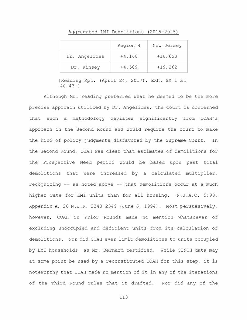
113
Aggregated LMI Demolitions (2015-2025)
Region 4 New Jersey
Dr. Angelides +4,168 +18,653
Dr. Kinsey +4,509 +19,262
[Reading Rpt. (April 24, 2017), Exh. SM 1 at 40-43.]
Although Mr. Reading preferred what he deemed to be the more
precise approach utilized by Dr. Angelides, the court is concerned
that such a methodology deviates significantly from COAH’s
approach in the Second Round and would require the court to make
the kind of policy judgments disfavored by the Supreme Court. In
the Second Round, COAH was clear that estimates of demolitions for
the Prospective Need period would be based upon past total
demolitions that were increased by a calculated multiplier,
recognizing -– as noted above -– that demolitions occur at a much
higher rate for LMI units than for all housing. N.J.A.C. 5:93,
Appendix A, 26 N.J.R. 2348-2349 (June 6, 1994). Most persuasively,
however, COAH in Prior Rounds made no mention whatsoever of
excluding unoccupied and deficient units from its calculation of
demolitions. Nor did COAH ever limit demolitions to units occupied
by LMI households, as Mr. Bernard testified. While CINCH data may
at some point be used by a reconstituted COAH for this step, it is
noteworthy that COAH made no mention of it in any of the iterations
of the Third Round rules that it drafted. Nor did any of the
114
iterations of the Third Round rules exclude the categories of units
deducted by Dr. Angelides. While it is noteworthy that Dr.
Angelides –- without using a multiplier -- produced an estimate
close to that endorsed by Dr. Kinsey, who more closely followed
the Second Round approach, the bottom line is simply that Dr.
Angelides deviated from the Second Round without convincing the
court that it was necessary to do so. And since that deviation
excludes units incorporated by COAH, Dr. Angelides’ approach
involves policy decisions that the court prefers to leave to
administrative consideration. Consequently, the court rejects the
modifications urged by Dr. Angelides.
The court, however, does endorse the recommendation of Mr.
Reading that all post-Sandy data be excluded from the averaging
process. Higher than normal demolitions occurred in more than the
four counties identified by Dr. Kinsey and for more years than the
two excluded by Dr. Angelides as a result of Hurricane Sandy. The
better approach to making an adjustment for the very high number
of demolitions in the wake of that disaster is thus to remove all
post-Sandy demolition data from the calculation of demolitions for
the Prospective need period. Moreover, given Dr. Kinsey’s
uncertainty about his close adherence to the Second Round in his
calculation of demolitions, the court instructed Mr. Reading to
follow COAH’s Second Round approach, utilizing the COAH
multiplier, but also incorporating the adjustment for Sandy data
115
he recommended. In addition, while Dr. Kinsey used county income
data in this step, the court directs Mr. Reading to use regional
LMI income data. Although COAH never defined what it meant by
“subregional” in its approach to calculating demolitions, N.J.A.C.
5:93-2.9, other steps in the methodology use regional and not
county incomes and the court has determined that regional income
data should be used in this step for consistency. As a result,
the court will incorporate into its statewide model total
demolitions during the Prospective Need period calculated by
Mr. Reading of 23,835 statewide and 4,947 for Region 4. For
Princeton the number of demolitions is 87, and for West Windsor
the figure is 53.
b. Residential conversions
While demolitions increase affordable housing need,
residential conversions represent the creation of new residential
units that COAH expected would reduce affordable housing need.
“Residential conversion is the creation of dwelling units from
already existing residential structures” that reduces municipal
need. N.J.A.C. 5:93-2.11, 26 N.J.R. 2320, 2349 (June 6, 1994).
Most conversions result from the creation of multiple smaller units
from larger existing units, and “[a]lmost all conversion consists
of additional dwelling units being created from other residential
units, and very rarely from nonresidential units.” 26 N.J.R. 2349
116
(June 6, 1994). COAH described the relationship between
demolitions and conversions in the Second Round:
Residential conversions to low- and moderate-income housing in normal markets are often on a par with demolitions for the low- and moderate-income sector. In stronger markets, conversions are more than demolitions; in weaker markets, less.
[Ibid.]
COAH further explained that because residential conversions are
closely related to the municipal percentage of two- to four-family
structures, conversions are calculated at the regional level and
then allocated to municipalities in proportion to their regional
share of two- and four-family dwellings. N.J.A.C. 5:93-2.11, 26
N.J.R. 2320, 2349 (June 6, 1994).
Residential conversions cannot be directly measured, but are
evidenced by the “unexplained difference” between the units
measured at the beginning and end of a period that cannot be
accounted for by building permits minus demolitions. Ibid. In
both the adopted Round 3.2 rules and the un-adopted Round 3.3
rules, COAH clarified this step by providing a clear mathematical
formula to estimate conversions, and changed the indicia of housing
construction from building permits, which were used in the Second
Round, to certificates of occupancy:
This methodology . . . defines residential conversions as the change in total units minus the difference between new construction (as indicated by certificates of occupancy) and

117
demolitions (as indicated by demolition permits).
[46 N.J.R. 985-86 (June 2, 2014).]
Notably, however, neither expert used COAH’s Third Round approach,
but tried to follow COAH’s Second Round to the extent they could
discern that methodology.
As with demolitions, COAH recognized in the Second Round that
“on a percentage basis, a greater share of residential conversion
units flows to the low- and moderate-income population than to the
population as a whole,” id. at 2349, but failed to designate a
specific multiplier to calculate conversions, differing from its
approach to demolitions in the Second Round. Given some ambiguity
in COAH’s Second Round approach, and the absence of a multiplier,
Drs. Angelides and Kinsey defaulted to the multiplier formula in
the Second Round used for demolitions, but selected different
datasets to use in their calculations. Dr. Angelides went on to
calculate the change in “occupied housing” using certificates of
occupancy to represent construction activity, while Dr. Kinsey
utilized building permits. Reading Rpt. (August 31, 2016), Exh. SW
4 at 63-69.
Dr. Angelides calculated the regional change in occupied
housing units by county between 2000 and 2010, using decennial
census data, and then aggregated the data to the appropriate
region. Dr. Angelides measured construction activity at the
municipal level for that period using certificates of occupancy
118
reported by NJDCA, concluding that they were a more reliable metric
of completed residential construction activity than building
permits, which might not result in actual construction in a given
year. Dr. Angelides likewise drew municipal demolition figures
from NJDCA data, and aggregated both construction activity and
demolition activity to the regional level to determine residential
conversions. Dr. Angelides then allocated the regional conversion
activity to municipalities in proportion to their share of regional
two- and four-family dwellings, utilizing 2009-2013 ACS data.
Finally, Dr. Angelides calculated the proportion of LMI conversion
activity for each municipality by utilizing 120 percent of the
proportion of households qualifying as LMI within each county, and
then projecting annualized conversion activity, by municipality,
into the Prospective Need period. Dr. Angelides estimated 2,025
LMI conversions in Region 4 and 11,662 statewide LMI conversions
for the Prospective Need period based on this approach.
Dr. Kinsey calculated the regional change in total housing
units at the county level, using 2000 decennial census and 2014
Population and Housing Unit Estimates data. Dr. Kinsey measured
construction activity for the same period using municipal building
permits reported by NJDCA, but adjusted for the effects of
Hurricane Sandy as he did when calculating demolitions in the
previous step. Dr. Kinsey then derived municipal demolitions from
NJDCA data, aggregating both construction activity and demolition

119
activity to the regional level to determine residential
conversions. Dr. Kinsey then allocated the regional conversion
activity to municipalities in proportion to their share of regional
two- and four-family dwellings in 2012, using 2010-2014 ACS data,
and estimated the LMI share of conversions based on 120 percent of
the proportion of households qualifying as LMI within each county,
capped at 95 percent, and then projected annualized conversion
activity, by municipality, into the Prospective Need period. Dr.
Kinsey’s calculations yielded a loss of 1,375 units in Region 4,
and a loss of 2,068 units statewide due to residential conversions,
which he attributed to the increased pricing of the converted
units. The following chart demonstrates a comparison of the results
recommended by each expert:
Impact of Aggregated LMI Conversions on Need (2015-2025)
Region 4 New Jersey
Dr. Angelides -2,025 -11,662
Dr. Kinsey +1,375 +2,068
Special Master Reading endorsed the use of certificates of
occupancy to represent building activity for the calculation of
residential conversions. Reading Rpt. (April 24, 2017), Exh. SM 1
at 47. Mr. Reading testified that economic conditions affecting
construction activity between 2000 and 2010 -- which includes the
onset of the Great Recession -- made building permits a less
120
reliable indicator of housing construction than certificates of
occupancy. He noted that, during this period, there were two
building permits issued for every housing unit ultimately
occupied, and that the State government issued two building permit
extensions in response to the effect on construction caused by the
economic downturn. Mr. Reading concluded, therefore, that
certificates of occupancy were a much better indicator of
construction activity than building permits in the Third Round.
Moreover, Mr. Reading was disturbed by the results of Dr. Kinsey’s
approach, which added units to need when COAH had always used
conversions to reduce need. Mr. Reading believed that Dr. Kinsey’s
reliance on building permits to measure construction activity was
a primary reason for the questionable results recommended by Dr.
Kinsey.
The court concurs with Mr. Reading that certificates of
occupancy provide a better indicia of housing construction for
this step, especially given the economic downturn that affected
the data available to the experts for the calculation of
conversions. Moreover, COAH recognized the superiority of using
certificates of occupancy in determining conversions in its
adopted Round 3.2 rules, and continued that approach in Round 3.3.
Whether or not Dr. Kinsey’s use of building permits skewed his
analysis, his results are inconsistent with COAH’s past
121
observations that residential conversions should reduce municipal
affordable housing need.
Although FSHC and the NJBA questioned the reliability of
certificates of occupancy by presenting evidence of individual
instances where municipalities did not accurately report and track
them, the practice did not appear to be widespread. Presumably,
those minor anomalies were known to COAH when it endorsed the use
of certificates of occupancy in Rounds 3.2 and 3.3. When weighed
against the shortcomings of building permits to reflect actual
construction activity, certificates of occupancy emerge as more
reliable despite the anomalies cited by Defendants. In addition,
Dr. Angelides’ residential conversion values not only decrease
affordable housing need, consistent with past COAH practice, but
are also less than both his and Dr. Kinsey’s demolition values,
which COAH anticipated would be the case in a weak housing market.
The court thus adopts Dr. Angelides’ approach for the calculation
of residential conversions as the best alternative based on the
trial record. His data will be included in the court’s model,
reducing affordable housing need by 11,662 statewide.
c. Filtering
Filtering is a secondary source adjustment that has proven
controversial in the past and remains controversial in the Third
Round. As noted above, Mr. Bernard endorsed most of Dr. Kinsey’s

122
model except for filtering, as did Judge Wolfson. In re Twp. Of S.
Brunswick, 448 N.J. Super. at 464.
Calculating filtering is an extremely complicated process
involving many variables. Days of testimony were devoted to each
expert’s attempt to explain and justify their models and the
results they produced, although Dr. Kinsey was skeptical about the
reliability of either model and questioned consideration of
filtering altogether as part of the fair share model. Two types
of filtering are proposed for inclusion in the current methodology.
Downward filtering reduces affordable housing need and occurs when
middle or upper income households vacate a housing unit, which
then becomes affordable to LMI households. Upward filtering
increases affordable housing need and occurs when a formerly
affordable housing unit rises in value beyond the reach of LMI
households. In prior rounds, downward filtering predominated,
with COAH recognizing filtering as the most significant market
force in reducing housing need. In re Adoption of N.J.A.C. 5:94 &
5:95, 390 N.J. Super. at 24. Although COAH maintained that
filtering takes place in all locations to some degree, COAH
asserted that it is found more often in urban and older suburban
areas with higher percentages of multifamily houses than in newer
suburban areas. 26 N.J.R. 2349 (June 6, 1994).
As the filtering concept evolved, COAH identified its
prerequisite market conditions. In the Second Round, COAH

123
described filtering as “a downward adjustment of housing” that was
“predicated on the existence of housing surpluses, which cause
housing prices to drop because of the excess of housing supply
over demand.” N.J.A.C. 5:93, Appendix A, 26 N.J.R. 2349 (June 6,
1994); N.J.A.C. 5:93-2.10. In response to comments on the Second
Round methodology, COAH identified five conditions that must exist
for filtering to occur: (1) an overall housing surplus; (2) a
surplus of new housing construction over new household formation;
(3) no major non-price barriers, such as discrimination, that
limit mobility among low-income households; (4) moderate operating
costs for newly built units; and (5) a limited number of poor
households. In re Adoption of N.J.A.C. 5:94 & 5:95, 390 N.J. Super.
at 42 (accepting COAH’s five conditions for the existence of
filtering in New Jersey, citing 36 N.J.R. 5801-5803 (December 20,
2004)). While the Appellate Division had upheld COAH’s First Round
filtering methodology because the legislative scheme was novel,
and the implementation of its goals was an evolving process, In re
Adoption of N.J.A.C. 5:94 & 5:95, 390 N.J. Super. at 44 (citing
Van Dalen v. Wash. Twp., 120 N.J. 234, 246 (1990)), the court’s
deference to COAH ultimately yielded to closer scrutiny.
Seventeen years later, the Appellate Division rejected COAH’s
use of filtering and the resulting reductions in Prospective Need
it had incorporated into the adopted Round 3.1 rules, questioning
the reasonableness of the data COAH relied upon. Id. at 41, 44-
124
45. Notably, in rejecting COAH’s application of filtering in Round
3.1, the Appellate Division declared that, “the legislative scheme
is no longer novel and COAH has had ample time to test its opinion
that filtering substantially reduces the need for affordable
housing in New Jersey.” Id. at 44.
The Appellate Division found that COAH had not adequately
demonstrated the existence of filtering according to the five
conditions it had previously articulated, finding as well that the
survey data used in the calculations did not represent “the most
recent and reliable data available.” Id. at 46. The Appellate
Division did not, however, invalidate filtering as a secondary
source altogether, but required that “[o]n remand, COAH must
consider more recent data relevant to whether the five conditions
for filtering currently exist in New Jersey, as well as any other
data supplied by the interested parties.” Ibid. In response to
this decision, COAH developed a new filtering model with the
assistance of Econsult, the firm retained by the municipalities to
assist them in this litigation. See N.J.A.C. 5:97, Appendix A, 97.
Notably, however, the Appellate Division did not address that
model’s validity when it rejected COAH’s Growth Share approach in
Round 3.2. In re Adoption of N.J.A.C. 5:96 & 5:97, 416 N.J. Super.
462, 511-12 (App. Div. 2010).
Dr. Angelides was skeptical that the five prerequisite
conditions were valid indicators of the existence of filtering,
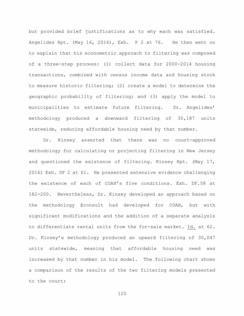
125
but provided brief justifications as to why each was satisfied.
Angelides Rpt. (May 16, 2016), Exh. P 2 at 76. He then went on
to explain that his econometric approach to filtering was composed
of a three-step process: (1) collect data for 2000-2014 housing
transactions, combined with census income data and housing stock
to measure historic filtering; (2) create a model to determine the
geographic probability of filtering; and (3) apply the model to
municipalities to estimate future filtering. Dr. Angelides’
methodology produced a downward filtering of 30,187 units
statewide, reducing affordable housing need by that number.
Dr. Kinsey asserted that there was no court-approved
methodology for calculating or projecting filtering in New Jersey
and questioned the existence of filtering. Kinsey Rpt. (May 17,
2016) Exh. DF 2 at 61. He presented extensive evidence challenging
the existence of each of COAH’s five conditions. Exh. DF.58 at
182-200. Nevertheless, Dr. Kinsey developed an approach based on
the methodology Econsult had developed for COAH, but with
significant modifications and the addition of a separate analysis
to differentiate rental units from the for-sale market. Id. at 62.
Dr. Kinsey’s methodology produced an upward filtering of 30,047
units statewide, meaning that affordable housing need was
increased by that number in his model. The following chart shows
a comparison of the results of the two filtering models presented
to the court:
126
Aggregated LMI Filtering (2015-2025)
Region 4 New Jersey
Dr. Angelides -7,777 -37,604
Dr. Kinsey +2,330 +30,047
Difference: 10,107 67,651
Special Master Reading rejected both Dr. Angelides’ and Dr.
Kinsey’s filtering approaches because they included “an abundance
of adjustments, probabilities, likelihoods, and extrapolations”
that he concluded were unreliable. Reading Rpt. (April 24, 2017),
Exh. SM 1 at 56. Given the extreme divergence between the
estimates prepared by the experts and absent a convincing
demonstration of their reliability, Mr. Reading recommended that
filtering not be included in the determination of fair share
obligations in the Third Round, agreeing with both Mr. Bernard and
Judge Wolfson on this issue.
Likewise, Mr. Bernard did not support the use of either
expert’s filtering approach. Mr. Bernard concluded that Dr.
Angelides’ approach was analogous to what had already been rejected
by the Appellate Division in In re Adoption of N.J.A.C. 5:94 &
5:95 By N.J. Council On Affordable Hous., 390 N.J. Super. at 42-
46, in that it represented an extremely complicated statistical
construct that supposedly demonstrated downward filtering effects
at the regional and local levels, while there was census data
127
demonstrating the opposite. And although he agreed with the
general upward direction of filtering reflected in Dr. Kinsey’s
data, Mr. Bernard also rejected his approach because it was equally
as complicated as that of Dr. Angelides, not transparent, and
contained questionable assumptions.
The court concurs with the recommendations of Mr. Reading and
Mr. Bernard, and the ruling of Judge Wolfson on this issue, and
rejects including filtering adjustments in the Third Round fair
share methodology. First and foremost, the court is not convinced
that either expert satisfactorily addressed the concerns expressed
by the Appellate Division in In re Adoption of N.J.A.C. 5:94 &
5:95, 390 N.J. Super. at 42-46. In that case, appellants argued
that COAH relied on flawed data to conclude that filtering was
occurring and the Appellate Division agreed, citing a failure of
COAH to demonstrate in the record that housing was becoming more
affordable and directing COAH, on remand, to substantiate the five
filtering conditions with recent relevant data. Ibid.
Here, even Dr. Angelides, a proponent of filtering
adjustments, nonetheless expressed some skepticism as to the
validity of COAH’s five filtering conditions. While presenting a
filtering model to the court, he provided scant statistical
evidence to accompany anecdotal indications that COAH’s conditions
had been satisfied. Angelides Rpt. (May 16, 2016), Exh. P2 at 76-
77. By contrast, Dr. Kinsey countered with credible testimony

128
providing a detailed analysis challenging each filtering condition
utilizing source documentation from COAH and other data to support
each point, yet he proceeded to advocate including his filtering
approach in his fair share model. Exh. DF 58 at 182-200. Mr.
Bernard also expressed skepticism regarding the existence of
filtering, based on census data indicating that housing has become
less affordable statewide. The record in this case thus provides
the court with little confidence that filtering is occurring in
New Jersey or, even if it is, that it can be measured in a reliable
manner.
The results advocated by the parties also are troubling to
the court. Notably, Dr. Angelides’ approach produced a number of
filtered housing units that were valued at hundreds of thousands
of dollars above COAH’s maximum LMI qualifying incomes, id. at
171-174, and Dr. Kinsey’s approach yielded a significant net upward
filtering, despite COAH’s observations in the Prior Rounds that
filtering generally could be expected to reduce housing need.
Consequently, the court has no confidence that either approach is
reasonable or reliable and thus will not include filtering as a
secondary source adjustment in its fair share methodology.
After addressing all of the steps discussed above, the court
directed Mr. Reading to calculate municipal secondary source
adjustments to reflect this court’s rulings, and also directed him
to aggregate all of the results to the State level for illustrative

129
purposes. The results are listed below with the recommendations
of the experts included for the sake of comparison:
Aggregated New Jersey Prospective Need 2015 – 2025
Angelides Kinsey Decision
Gross Prospective Need
54,140 138,471 73,209
Secondary Sources Demolitions
+18,653 +19,262 +23,835
Conversions -11,662 +2,068 -11,662
Filtering -37,604 +30,047 0,000
Prospective Need 23,527 189,848 85,382
d. Reallocation of Secondary Source Adjustments
Dr. Angelides testified that COAH’s Second Round methodology
was defective due to what he called the “zero bound” flaw, whereby
credit for excess affordable housing in individual municipalities
is effectively lost because it is not pooled and reallocated to
other municipalities in the region. According to Dr. Angelides,
COAH calculated secondary source adjustments in the Second Round
by region and allocated them down to individual municipalities,
which can result in a net negative need. Angelides Rpt. (May 16,
2016), Exh. P 2 at 82-83. Such negative need could occur when the
number of housing units created through conversions and filtering
is greater than the need for units created by demolitions and
filtering. Dr. Angelides noted that once this secondary source
negative need is allocated to the municipalities, it is applied
130
first against any Prospective Need the municipality may have, and
then against municipal Present Need. Dr. Angelides pointed out
that a municipality could have a secondary source negative need
that is larger than the sum of its Prospective Need and Present
Need, meaning that the municipality has more affordable housing
than its fair share of the region’s affordable housing need. Dr.
Angelides noted that, under COAH’s Second Round practice, a net
negative need (excess available affordable housing) is not
otherwise accounted for and is set to zero. Ibid. Dr. Angelides
argued that instead of being zeroed out and lost, municipal
negative need should be aggregated back to the region, pooled, and
reallocated to offset the remaining affordable housing need of the
region’s other municipalities. Ibid. Dr. Angelides’ secondary
source reallocation step would add over 30,000 units of affordable
housing statewide, decreasing the need by that number. Under Dr.
Angelides’ approach, over 5,500 additional affordable housing
units would be reallocated to Region 4.
Notably, however, any excess municipal affordable housing
(negative need) is not lost, but can be credited in future fair
share rounds in the compliance process. Mr. Bernard testified
that, in the Prior Rounds, municipalities with surplus housing
units from a previous round were credited with those units in the
subsequent round. Indeed, the Second Round rules state that,
“[t]he reduction for prior-cycle activities is subtracted from

131
Pre-credited Need; it cannot reduce Pre-credited Need below zero.
Any unexpended reduction is carried over to the next cycle.” 26
N.J.R. 2350 (June 6, 1994). And in fact, in Mercer County
settlements reviewed by this court, some municipalities are using
excess credits from the past toward satisfaction of their Third
Round obligations, consistent with past COAH practice.
Thus, the court concludes that any surplus affordable housing
units in individual municipalities can be utilized in subsequent
fair share rounds so that there is no need to deviate from prior
COAH practice and reallocate any surplus here. Also, the addition
of a secondary source reallocation step to the fair share
methodology is the type of policy decision that is better left to
an administrative agency that can thoroughly review any such change
through rulemaking. This court therefore declines to adopt Dr.
Angelides’ secondary source reallocation. The court does note,
however, that Dr. Angelides’ results for this proposal were greatly
affected by incorporation of his filtering model, which was also
rejected by the court.
e. Calculate Prospective Need by Municipality
The next step in calculating Prospective Need is to adjust
each municipality’s gross Prospective Need to reflect secondary
source adjustments of supply and demand. Having excluded filtering
from this adjustment, the court –- following Prior Round
methodology -- directed Mr. Reading to calculate municipal
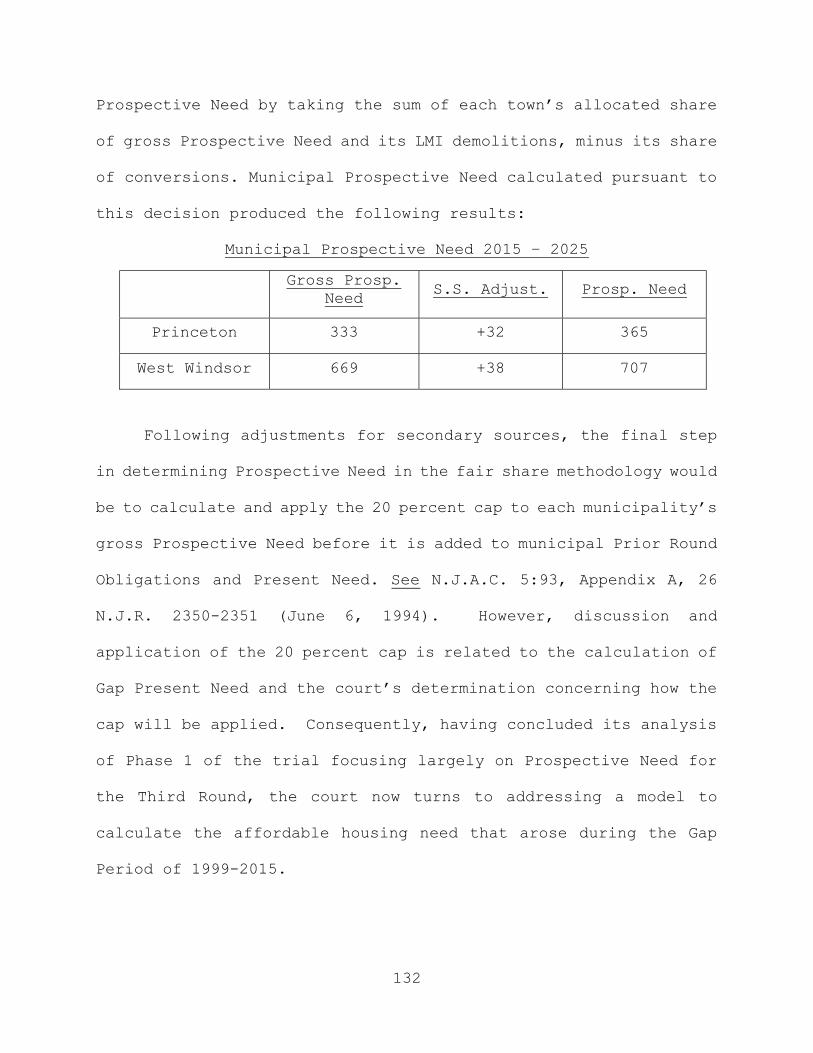
132
Prospective Need by taking the sum of each town’s allocated share
of gross Prospective Need and its LMI demolitions, minus its share
of conversions. Municipal Prospective Need calculated pursuant to
this decision produced the following results:
Municipal Prospective Need 2015 – 2025
Gross Prosp. Need
S.S. Adjust. Prosp. Need
Princeton 333 +32 365
West Windsor 669 +38 707
Following adjustments for secondary sources, the final step
in determining Prospective Need in the fair share methodology would
be to calculate and apply the 20 percent cap to each municipality’s
gross Prospective Need before it is added to municipal Prior Round
Obligations and Present Need. See N.J.A.C. 5:93, Appendix A, 26
N.J.R. 2350-2351 (June 6, 1994). However, discussion and
application of the 20 percent cap is related to the calculation of
Gap Present Need and the court’s determination concerning how the
cap will be applied. Consequently, having concluded its analysis
of Phase 1 of the trial focusing largely on Prospective Need for
the Third Round, the court now turns to addressing a model to
calculate the affordable housing need that arose during the Gap
Period of 1999-2015.

133
V. Gap Present Need/Phase 2
A. Gap Present Need Factual and Procedural History
In the Ocean County proceeding to determine the methodology
for establishing the fair share affordable housing obligations for
thirteen Ocean County municipalities, the Honorable Mark A.
Troncone, J.S.C., raised the issue of whether Third Round housing
obligations should include the need that arose from the expiration
of the Second Round rules in 1999 to the date in 2015 by which
towns were required to file declaratory judgment actions to
demonstrate constitutional compliance and to obtain immunity from
builders’ remedy lawsuits. See Mount Laurel V, 227 N.J. at 516.
This period has become known as the “gap,” representing the sixteen
years in which COAH did not adopt a full set of Third Round rules
that passed constitutional muster. The Ocean County
municipalities, joined by the League of Municipalities, argued to
Judge Troncone that fair share obligations could only fall into
the two well-defined components of Present Need and Prospective
Need, claiming that since any gap need fell outside of these
categories, establishing a fair share for this period would violate
the FHA. Ibid. FSHC, NJBA, and private developers opposed this
argument and joined in asserting that gap need must be captured as
part of a town’s affordable housing obligation. Mount Laurel V,
227 N.J. at 516-17.

134
The same experts who submitted reports regarding Prospective
Need provided reports to Judge Troncone and to court-appointed
Special Master Reading, analyzing whether and then how gap need
could be calculated as part of a municipality’s Third Round fair
share obligation. The League of Municipalities’ expert, Dr.
Angelides, asserted that there was no “legally defined obligation”
to address gap need for the Third Round cycle, Mount Laurel V, 227
N.J. at 517, while Mr. Bernard, on behalf of NJBA, claimed that
COAH’s regulations, as well as the reality of affordable housing
need in New Jersey, mandated that the gap need be included in a
Prospective Need analysis. Ibid. FSHC’s expert, Dr. David Kinsey,
contended that COAH’s regulations and applicable case law required
including the gap period need in the Third Round, either separately
or as part of the Prospective Need component, which he asserted
spanned the entire period from 1999 to 2025. Ibid. Special Master
Reading reviewed all of the submitted reports and recommended to
Judge Troncone that gap period need should be calculated as a
“separate and discrete” methodology unique to the gap period,
rather than as part of Prospective Need. Ibid.
On February 18, 2016, Judge Troncone issued an opinion
concluding that the housing need that arose during the gap period
must be included as part of the Third Round fair share obligation
in order to satisfy constitutional requirements. Judge Troncone
also held that gap period need was not part of Prospective Need,

135
but should be calculated as a “separate and discrete component” of
need, based on actual growth during the 1999-2015 period, rather
than on future projections. See Mount Laurel V, 227 N.J. at 518-
19 (summarizing the proceedings before the trial court in Ocean
County). The Township of Barnegat appealed Judge Troncone’s ruling
that a gap period component must be included in the Third Round.
Ibid. The Appellate Division, at the direction of the Supreme
Court, expedited the appellate proceedings after the Court denied
FSHC’s emergent application for direct certification. Ibid.
On July 11, 2016, the Appellate Division issued its ruling,
captioned In re Declaratory Judgment Actions filed by Various
Muns., Cty. Of Ocean, 446 N.J. Super. 259 (App. Div. 2016) (“Ocean
County Appeal”), which found that there was no basis in the FHA or
otherwise to require municipalities to retroactively calculate a
new “separate and discrete” affordable housing obligation during
the gap period. Id. at 267-68. The Appellate Division grounded
its decision in Mount Laurel IV and the FHA and viewed the creation
of a “separate and discrete” gap component as over-reaching
policymaking best left to the Legislative and Executive branches.
Ibid. In rejecting Judge Troncone’s approach to the retrospective
calculation of the need that arose during this period, however,
the Appellate Division emphasized that some gap period need could
be captured in a municipality’s calculation of Present Need. Ocean
County Appeal, 446 N.J. Super. at 295.
136
FSHC moved to stay the decision pending expedited review by
the Supreme Court, which the Appellate Division denied on July 18,
2016. FSHC then applied to the Supreme Court for leave to appeal
and a stay, both of which were ultimately granted on September 8,
2016. Barnegat remained the only municipality involved in the
appeal insofar as it challenged the obligation to account for any
need that arose during the gap period. Mount Laurel V, 227 N.J. at
520-21. On January 18, 2017, during the pendency of the Mercer
County methodology trial, the Supreme Court affirmed and modified
the Appellate Division’s decision, ordering that gap period
affordable housing need be included as part of the fair share
component of Present Need, in what has become known as Mount Laurel
V, 227 N.J. at 513-14.
In response to Mount Laurel V, on January 31, 2017, this court
added a Gap Present Need phase to the methodology trial and
scheduled it to follow the conclusion of the “Prospective Need”
phase, already in progress. The court again directed the experts
to develop, exchange, and submit methodology reports to Mr. Reading
and to the court. Given the guidance provided by the Supreme
Court, this court urged the parties to work together in fashioning
a mutually acceptable methodology to address the calculation of
Gap Present Need. Unfortunately, the parties resisted the court’s
efforts, appearing to be too invested in their own methodological
paradigms to embrace a joint approach. The challenges presented
137
by crafting a model to determine Gap Present Need are underscored
by the continually evolving positions of the experts, starting
with their submissions to Judge Troncone and continuing through
the testimony and evidence presented at the Mercer County
methodology trial. See also Mount Laurel V, 227 N.J. at 522 (noting
how the arguments regarding gap need had evolved throughout the
proceedings before the Supreme Court).
Dr. Kinsey testified that he felt bound to follow the same
approach for Gap Present Need that he had utilized for determining
Prospective Need. To support this approach, he cited COAH’s use
of Prospective Need methodology when it recalculated the fair share
obligations assigned to municipalities in the First Round when
they proved to be too high. COAH called this process Prior–Cycle
Prospective Need, described at N.J.A.C. 5:93-1.3, and discussed in
Mount Laurel V, 227 N.J. at 528, fn.7. Dr. Kinsey thus endorsed
a retrospective prospective need analysis, similar to what he had
submitted to Judge Troncone. Notably, however, Dr. Kinsey had
submitted a different approach to Judge Wolfson in the South
Brunswick case after the Appellate Division decision had issued,
but before it was modified by the Supreme Court. That approach
was similar to what Dr. Angelides advocated in the Mercer trial.
On the other hand, Dr. Angelides rejected reliance on past
COAH practice given the new and unique circumstances presented by
Gap Present Need. He calculated the number of LMI households
138
formed during the gap and still in existence at the end of the gap
period and then reduced that number by removing categories of
households in response to comments in the Supreme Court’s decision.
Oddly enough, although Dr. Angelides had criticized the
methodology developed by Dr. Kinsey and submitted to Judge Wolfson
in the South Brunswick case, he adopted a similar approach
following the Supreme Court’s decision. Unsurprisingly, the
calculations of Gap Present Need advocated by the two experts were
wildly divergent, with Dr. Kinsey endorsing a much higher number
than that advocated by Dr. Angelides. In that sense, their
positions relative to each other mirrored the conclusions they had
advanced in the Prospective Need phase of the trial.
Mr. Bernard once again endorsed the approach developed by Dr.
Kinsey, with several modifications, including the same rejection
of a filtering adjustment that he had recommended in Phase 1 of
the trial. Notably, after listening to the testimony of Dr.
Angelides, he went even further and accepted a variation on one of
the adjustments advocated by Dr. Angelides.
Mr. Reading also changed his position from the one he had
advocated before Judge Troncone, and then refined his
recommendations after listening to the testimony presented during
Phase 2 of the trial. Although he largely supported the method
presented by Dr. Angelides, he rejected or modified some of the
adjustments contained in that model. As noted above, this lack of

139
consensus reflected the divergent results advocated by the parties
in the first phase of the trial, leading to thirteen days of
additional testimony between May 15, 2017 and June 19, 2017. Once
again the court appreciated the assistance of Mr. Reading in
reviewing the two different proposed gap methodologies from a
neutral perspective.
B. Gap Present Need Legal Standard
The Mount Laurel V decision explicitly requires that gap
period need be included as part of the fair share affordable
housing methodology and places it within the calculation of Present
Need. 227 N.J. at 529-531. Although the Supreme Court neither
defined a specific methodology to calculate gap period need, nor
expressed a preference for any of the proposed approaches that had
been submitted to Judge Troncone, it did provide additional
guidance for the trial courts. Firstly, the Supreme Court was
unequivocal in declaring that any fair share methodology must
include gap period need:
As to the fundamental disagreement—whether the gap period must be addressed—we waste no time in settling that issue. There is no fair reading of this Court's prior decisions that supports disregarding the constitutional obligation to address pent-up affordable housing need for low- and moderate-income households that formed during the years in which COAH was unable to promulgate valid Third Round rules.
[Mount Laurel V, 227 N.J. at 521.]
140
The Court reiterated in unmistakable terms that there would be “no
hiatus in the constitutional obligation.” Id. at 522. It then
directed that the calculation of gap need be addressed by the trial
courts as part of the judicial effort to ensure compliance by New
Jersey’s municipalities with their constitutional obligations:
We conclude, as did the Appellate Division panel and the trial court, that the need of presently existing low- and moderate-income households formed during the gap period must be captured and included in setting affordable housing obligations for towns that seek to be protected from exclusionary zoning actions under the process this Court has set up while COAH is defunct . . .
[Mount Laurel V, 227 N.J. at 529 (internal citations omitted).]
Having identified the need, however, the Court then had to
determine how to incorporate gap need into the fair share
methodology. In considering the options, the Supreme Court agreed
with the Appellate Division that including gap need within
Prospective Need was untenable. Indeed, the Court observed that
the very category was “a more or less calcified term . . . ,”
having been defined in the FHA and in COAH’s rules as purely
forward looking. As a result, the Court found that it would be
inappropriate to incorporate a retrospective calculation—-
necessary for gap need—-into a category based on projections,
concluding that:
[b]y . . . definition, [P]rospective [N]eed is forward looking. It is predictive—a projection of future need. The statutory language was not

141
designed to account for past periods of time when performing a calculation of anticipated housing need for low- and moderate-income households.
[Mount Laurel V, 227 N.J. at 526-27.]
Instead, following the suggestion of the Appellate Division,
the Supreme Court concluded that of the available categories, only
Present Need had “the potential to capture pent-up housing need
that arose during the sixteen-plus years of the gap period and
that continues to be an identifiable category of housing need that
experts could flesh out.” Mount Laurel V, 227 N.J. at 526 (citing
Ocean County Appeal, 446 N.J. Super. at 294-95). In arriving at
that conclusion, the Court recognized that prior practice limited
the concept of Present Need to identifying substandard and
overcrowded existing housing units at a single point in time—-the
start of the next affordable housing cycle. Nonetheless, the Court
determined that the category could be expanded to address
calculation of the need for affordable housing of the LMI
households that formed between 1999 and 2015 and still needed such
housing at the end of that period, which coincided with the
beginning of the Third Round fair share cycle. The Supreme Court
noted that because the term Present Need was not defined in the
FHA, it was malleable and could be adapted to address gap period
need (hereinafter referred to as “Gap Present Need”). Mount Laurel
V, 227 N.J. at 529. While directing that Gap Present Need be added
to the fair share methodology to determine municipal affordable

142
housing obligations, the Court explicitly refused to endorse any
of the analytical approaches and characteristics of Gap Present
Need calculations presented to Judge Troncone:
[T]his Court is not adopting any particular party's expert's opinion on such characteristics, which are a matter of dispute. Rather, we find the phrase useful only to describe the practice in which the experts will have to engage to convince the trial courts as to what characteristics should be included when providing a fair estimate of the need that arose during the gap period and remains unmet today.
[Mount Laurel V, 227 N.J. at 530, n.8.]
The Supreme Court did, however, provide guidance to assist the
trial courts in determining this “fair estimate”:
The trial courts must take care to ensure that the present need is not calculated in a way that includes persons who are deceased, who are income-ineligible or otherwise are no longer eligible for affordable housing, or whose households may be already captured through the historic practice of surveying for deficient housing units within the municipality.
[Mount Laurel V, 227 N.J. at 531.]
The focus of Gap Present Need on the unmet housing need of
LMI households formed between 1999 and 2015 might at first blush
appear to pose an easier task for a trial court considering the
matter in 2017-2018 than the calculation of Prospective Need, which
is based on projections and is inherently speculative in nature.
Somewhat unexpectedly, therefore, Gap Present Need confronted the
court with complexities borne of the lack of existing datasets to

143
pinpoint the need, and with conflicting methodologies advocated by
the experts that were even more divergent than in the analysis of
Prospective Need.
It quickly became apparent that even though real data was
available for the gap period and projections could be avoided,
getting a handle on the number of LMI households that formed in
the gap period and were still in need of affordable housing in
2015 was extremely challenging. Moreover, while placing gap need
within the broader category of Present Need, the calculation of
gap need was quite distinct from traditional Present Need. As
noted above, whereas traditional Present Need counts deficient
housing units and is addressed through the rehabilitation of those
units, Gap Present Need is measured in LMI households and adds to
a new construction obligation.
While the Supreme Court chose Present Need as the context for
gap period need because Present Need is not defined in the FHA and
therefore provided flexibility in fashioning an appropriate
methodology, the absence of clear precedent or COAH rules on the
subject has made the task more demanding. Although the Supreme
Court’s admonition to the trial courts when addressing Prospective
Need to utilize the most up-to-date and appropriate data and to
avoid policy-making better left to the Legislative and Executive
branches continues to offer some guidance for determining Gap
Present Need, those guidelines simply are more difficult to apply

144
when addressing a new category of need based on unprecedented
circumstances. Yet, as the Supreme Court did not shy away from
requiring numerical obligations to be calculated for Prospective
Need despite the acknowledged difficulty in making multiple
projections into the future, Mount Laurel II, 92 N.J. at 257, so
the complexities involved in determining Gap Present Need did not
deter the Court from requiring the trial courts to calculate
numerical “fair estimates” of that Need. Mount Laurel V, 227 N.J.
at 528-521. So it is with more than a little trepidation that the
court approaches the task at hand.
C. Summary of Methodological Approaches
Lacking clearly applicable precedent from COAH or
prescription of a specific methodology from the New Jersey
appellate courts, Drs. Angelides and Kinsey enjoyed wider latitude
in devising their Gap Present Need methodology than they did for
determining Prospective Need. Nonetheless, Dr. Angelides and Dr.
Kinsey both began their Gap Present Need calculations by estimating
LMI household growth during the gap period, essentially following
their Prospective Need approaches. Where the two experts diverged
was in how they estimated LMI Household Growth, the very different
adjustments they applied to account for their interpretations of
the guidance provided in Mount Laurel V, and the way in which they

145
each allocated and incorporated their Gap Present Need obligations
into the existing fair share methodology.
1. Dr. Angelides (for the municipalities)
a. Guiding Principles
Dr. Angelides interpreted Mount Laurel V as requiring that he
develop a novel approach to calculate the newly defined Gap Present
Need that required consideration of the current housing status of
Gap Period LMI Households. Angelides Gap Rpt. (April 12, 2017),
Exh. P 86 at 9. According to Dr. Angelides, both the Appellate
Division’s gap decision and Mount Laurel V made clear that Gap
Present Need is not a “separate and discrete” component of need
that can be captured by a retrospective Prospective Need
methodology under the FHA. Ibid. (citing Mount Laurel V, 227 N.J.
at 519-520). Dr. Angelides asserted that under Mount Laurel V, no
prior fair share method was adequate to capture need under the
unique circumstances of the gap period. Dr. Angelides specifically
rejected the use of the Second Round Prior-Cycle Prospective Need
recalculation of First Round obligations because he concluded that
it failed to consider current housing circumstances. Angelides Gap
Rpt. (April 12, 2017), Exh. P 86 at 9. In that process COAH had
recalculated First Round Prospective Need obligations on a
retrospective basis to correct for over-projections before unmet
First Round need was incorporated into Second Round obligations.
See N.J.A.C. 5:93-2.8, Appendix A, 26 N.J.R 2348 (June 6, 1994),
146
and Comment 6, 26 N.J.R. 2302 (June 6, 1994). As a result, COAH
dampened down Prior Cycle Prospective Need by 48 percent to provide
a mid-period (1990) correction. Ibid.
Dr. Angelides claimed that, unlike in Mount Laurel IV where
the Supreme Court had directed the trial courts to follow Prior
Round COAH practices, the Supreme Court in Mount Laurel V offered
trial judges “considerable flexibility” to utilize new methods
when crafting Gap Present Need methodologies. Angelides Gap Rpt.
(April 12, 2017), Exh. P 86 at 11. Dr. Angelides outlined four
“common and central principles” he derived from Mount Laurel V:
(1) “Gap Present Need households must have been added during the
gap period,” (2) “Gap Present Need households must currently be
LMI and otherwise eligible for affordable housing” (excludes Gap
Period LMI Households still living in the state with significant
assets), (3) “Gap Present Need households must not be represented
within the traditional quantification of Present Need” (excludes
Gap Period LMI Households living in overcrowded or deficient
housing), and (4) “Gap Present Need households must currently have
an identifiable need for affordable housing” (excludes Gap Period
LMI Households that live in affordable housing). Id. at 6-8.
b. Methodological Approach
Dr. Angelides utilized what he termed a “single snapshot”
approach, making his calculations of LMI household growth and
associated reductions at a single point in time, that being the
147
end of the gap period in 2015. He consciously sought to mimic the
aspect of traditional Present Need that estimates existing
deficient units as a “snapshot” of current need within a
municipality, even utilizing that term -- which had been employed
by the Supreme Court to describe traditional Present Need -- in
his gap analysis. See Mount Laurel V, 227 N.J. at 527. Since both
he and Dr. Kinsey accepted the same updated estimates of total
households for 1999 and 2015 from datasets published by the United
States Census Bureau, concluding that total households in New
Jersey increased by 187,390 households during the gap period, the
multi-step total household growth calculations of the Prospective
Need phase were not necessary for either expert. Reading Final Gap
Rpt. (June 12, 2017), Exh. SM 11 at 4.
Dr. Angelides started his “single snapshot” approach by
taking the increase in total households over the gap period and
applying ratios that he calculated to show the percentage of that
total that qualified as LMI in 2015. This method contrasted with
the methodology employed by Dr. Kinsey, which estimated the number
of LMI households in 1999 and 2015, and then calculated the
difference between the two. Dr. Angelides utilized true median
incomes in his analysis, as he had done in his Prospective Need
methodology. Ibid. That process yielded a growth in LMI households
in the gap period of 73,213 LMI households, which is 39.07 percent
of the total household growth during the period. He then adjusted
148
his total LMI household number by removing those gap period LMI
households that were living in affordable housing, possessed
significant assets, or that overlapped with units captured as part
of traditional Present Need as of 2015. Id. at 11-12. Dr.
Angelides allocated this regional-level Gap Present Need to
municipalities utilizing the same four allocation factors from his
Prospective Need approach. Angelides Gap Rpt. (April 12, 2017),
Exh. P 86 at 43. He then added his Gap Present Need for each
municipality to his previously calculated municipal Prospective
Need before applying the 20 percent caps on new construction
obligations.
Angelides New Jersey Gap Present Need 1999-2015 (pre-cap)
Growth Rate Calculation
Total HH Growth 187,390
LMI HH Growth Rate 39.07%
LMI HH Growth 73,213
Calculation of Adjustments
In Affordable Housing 27,720
Significant Assets 1,958
Present Need Overlap + 3,992
Total Adjustments 33,670
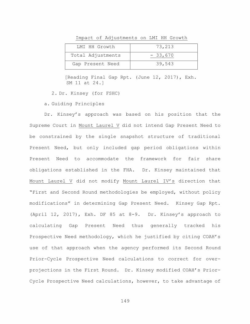
149
Impact of Adjustments on LMI HH Growth
[Reading Final Gap Rpt. (June 12, 2017), Exh. SM 11 at 24.]
2. Dr. Kinsey (for FSHC)
a. Guiding Principles
Dr. Kinsey’s approach was based on his position that the
Supreme Court in Mount Laurel V did not intend Gap Present Need to
be constrained by the single snapshot structure of traditional
Present Need, but only included gap period obligations within
Present Need to accommodate the framework for fair share
obligations established in the FHA. Dr. Kinsey maintained that
Mount Laurel V did not modify Mount Laurel IV’s direction that
“First and Second Round methodologies be employed, without policy
modifications” in determining Gap Present Need. Kinsey Gap Rpt.
(April 12, 2017), Exh. DF 85 at 8-9. Dr. Kinsey’s approach to
calculating Gap Present Need thus generally tracked his
Prospective Need methodology, which he justified by citing COAH’s
use of that approach when the agency performed its Second Round
Prior-Cycle Prospective Need calculations to correct for over-
projections in the First Round. Dr. Kinsey modified COAH’s Prior-
Cycle Prospective Need calculations, however, to take advantage of
LMI HH Growth 73,213
Total Adjustments - 33,670
Gap Present Need 39,543
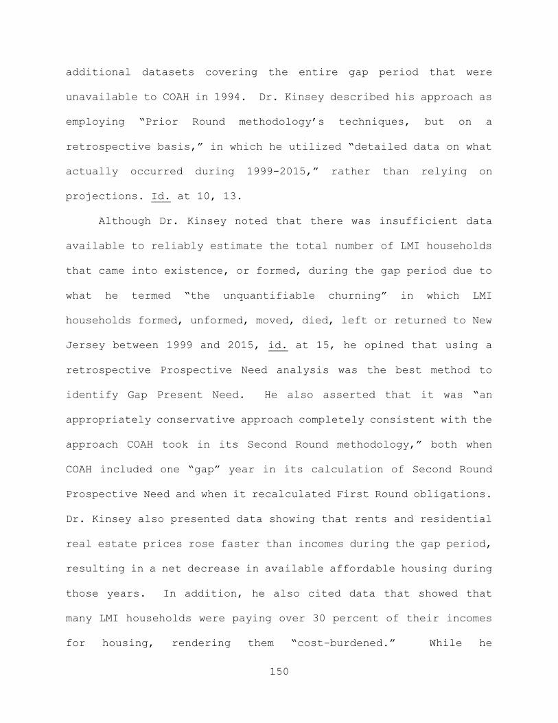
150
additional datasets covering the entire gap period that were
unavailable to COAH in 1994. Dr. Kinsey described his approach as
employing “Prior Round methodology’s techniques, but on a
retrospective basis,” in which he utilized “detailed data on what
actually occurred during 1999-2015,” rather than relying on
projections. Id. at 10, 13.
Although Dr. Kinsey noted that there was insufficient data
available to reliably estimate the total number of LMI households
that came into existence, or formed, during the gap period due to
what he termed “the unquantifiable churning” in which LMI
households formed, unformed, moved, died, left or returned to New
Jersey between 1999 and 2015, id. at 15, he opined that using a
retrospective Prospective Need analysis was the best method to
identify Gap Present Need. He also asserted that it was “an
appropriately conservative approach completely consistent with the
approach COAH took in its Second Round methodology,” both when
COAH included one “gap” year in its calculation of Second Round
Prospective Need and when it recalculated First Round obligations.
Dr. Kinsey also presented data showing that rents and residential
real estate prices rose faster than incomes during the gap period,
resulting in a net decrease in available affordable housing during
those years. In addition, he also cited data that showed that
many LMI households were paying over 30 percent of their incomes
for housing, rendering them “cost-burdened.” While he

151
acknowledged that neither COAH nor the courts had ever included a
calculation of cost-burdened LMI households in fair share
methodologies, he asserted that testimony on this subject was
necessary to provide an important “context” for the court’s
consideration of Gap Present Need.
b. Methodological Approach
For his Gap Present Need calculations, Dr. Kinsey reprised
his multi-step Prospective Need methodology, beginning with the
same incremental “two snapshots” approach he had used to calculate
LMI household growth previously. Reading Final Gap Rpt. (June 12,
2017), Exh. SM 11 at 6. Dr. Kinsey estimated the growth of LMI
households during the gap period by calculating the number of LMI
households at the beginning and end of the gap period using the
same HUD/COAH-derived income grids he had employed in Phase 1 of
the trial. Id. at 7. Continuing his Prospective Need approach,
Dr. Kinsey pooled and reallocated gap period LMI household growth
for working age households to regions that experienced recent job
growth. Kinsey Gap Rpt. (April 12, 2017), Exh. DF 85 at 75. Dr.
Kinsey then allocated his regional LMI household growth to the
municipalities, exempting urban aid municipalities, so that he
could then apply secondary source adjustments for demolitions,
conversions and filtering that occurred during the gap period.
Reading Final Gap Rpt. (June 12, 2017), Exh. SM 11 at 5-7, 11.
Dr. Kinsey then added these municipal Gap Present Need obligations
152
to his previously calculated municipal Unmet Prior Round
Obligations, Present Need, and Prospective Need. Ibid. However,
Dr. Kinsey advocated applying 20 percent caps to Prospective Need
and Gap Present Need estimates separately before adding those
numbers together with the other categories of Third Round
obligations.
Kinsey New Jersey Gap Present Need 1999-2015
Total HH Growth 187,390
LMI HH Growth Rate 49.87%
LMI HH Growth 93,451
Secondary Source Adjustments
Demolitions 37,050
Filtering 44,263
Conversions 15,408
Less Urban Aid (40,347)
Total Adjustments 56,374
Calculating Gap Present Need
LMI HH Growth 93,451
Total Adjustments 56,374
Gap Present Need 149,825
[Ibid. at 24 (emphasis added).]
3. Mr. Bernard (for NJSBA)
Mr. Bernard generally supported Dr. Kinsey’s Gap Present Need
approach, with some modifications, and was very critical of the

153
methodology advocated by Dr. Angelides. Mr. Bernard agreed with
Dr. Kinsey that a “two snapshot” approach was appropriate because
it considered housing activity over the entire gap period. Like
Dr. Kinsey, Mr. Bernard advocated following COAH’s Second Round
Prior-Cycle Prospective Need approach for calculating Gap Present
Need. Bernard Gap Rpt. (April 12, 2017), Exh. DB 46 at 2. However,
unlike Dr. Kinsey, Mr. Bernard would have applied secondary source
adjustments for only conversions and demolitions, having deemed
the use of filtering to have been overturned by the Appellate
Division and not being convinced that any filtering methodology
proposed in this case satisfied the Appellate Division’s concerns.
Bernard Gap Response Rpt. (April 24, 2017), Exh. DB 47 at 1. Mr.
Bernard also suggested modifications to Dr. Kinsey’s calculation
of conversions and treatment of the Highlands area of New Jersey.
He strongly criticized Dr. Angelides’ rejection of the HUD/COAH-
derived grids to establish LMI incomes, pointing out that this
approach greatly reduced the Gap Present Need estimates. Mr.
Bernard likewise rejected the adjustments made by Dr. Angelides to
reduce the overall gap need, Bernard Gap Rpt. (April 12, 2017),
Exh. DB 46 at 7, although he eventually did accept making some
modified adjustment to Dr. Angelides’ calculation for the overlap
with traditional Present Need.
While Mr. Bernard initially rejected the adjustment advocated
by Dr. Angelides to prevent the overlap identified by the Supreme
154
Court with traditional Present Need, Mount Laurel V, 227 N.J. at
529-530, he later conceded in testimony that a Present Need overlap
adjustment could have merit. He qualified his endorsement of this
reduction, however, noting that it should not include Present Need
in urban aid municipalities because they do not receive new
construction obligations under the fair share methodology. Mr.
Bernard also agreed with Dr. Kinsey in rejecting the reduction
taken by Dr. Angelides for LMI households living in affordable
housing because it was impossible to ascertain which of those
households were formed during the gap period, such an adjustment
could lead to double-counting when municipalities take bonus
credits for the construction of affordable units in the gap period
during the compliance process, and because of the marked increase
in cost-burdened LMI households during the gap period. Bernard Gap
Rpt. (April 12, 2017), Exh. DB 46 at 13, 18.
4. Special Master Reading
Special Master Reading generally agreed with the Gap Present
Need approach proposed by Dr. Angelides, rejecting Dr. Kinsey’s
Prospective Need methodology that he had favored in the Ocean
County proceedings because it appeared less responsive to the
concerns articulated by the Supreme Court in Mount Laurel V. Mr.
Reading testified that although Dr. Kinsey’s use of an incremental
Prospective Need methodology was not unreasonable, Dr. Angelides’
approach directly addressed the new and unique circumstances of
155
Gap Present Need. In particular, Mr. Reading agreed with Dr.
Angelides that his single snapshot approach to calculating gap
period LMI household growth was more consistent with the point-
in-time analysis of traditional Present Need, and more
appropriately responded to the Supreme Court’s Mount Laurel V
decision.
Mr. Reading recommended Dr. Angelides’ Gap Present Need
methodology, but with modified adjustments. Mr. Reading concluded
that the significant asset test should not be used to adjust Gap
Present Need for the same reasons he rejected the test in Phase 1
of the trial. While he viewed the test as reasonable, he deemed
it to reflect a policy determination that should only be endorsed
as part of a comprehensive re-evaluation of the fair share
methodology by an administrative agency that would examine many
considerations and not just this one policy change in isolation.
In addition, Mr. Reading recommended that LMI households living in
deed-restricted affordable housing should not be excluded from Gap
Present Need because municipalities may already have either been
given bonus credits for those units, or may be applying for credits
for those units during the ongoing Third Round compliance process.
The adjustment made by Dr. Angelides in removing such households
could thus lead to a double reduction in the obligation in many
towns, improperly diluting their fair share obligations. Indeed,
the court confirms that several Mercer County municipalities that
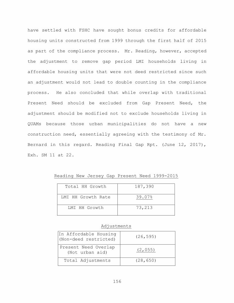
156
have settled with FSHC have sought bonus credits for affordable
housing units constructed from 1999 through the first half of 2015
as part of the compliance process. Mr. Reading, however, accepted
the adjustment to remove gap period LMI households living in
affordable housing units that were not deed restricted since such
an adjustment would not lead to double counting in the compliance
process. He also concluded that while overlap with traditional
Present Need should be excluded from Gap Present Need, the
adjustment should be modified not to exclude households living in
QUAMs because those urban municipalities do not have a new
construction need, essentially agreeing with the testimony of Mr.
Bernard in this regard. Reading Final Gap Rpt. (June 12, 2017),
Exh. SM 11 at 22.
Reading New Jersey Gap Present Need 1999-2015
Total HH Growth 187,390
LMI HH Growth Rate 39.07%
LMI HH Growth 73,213
Adjustments
In Affordable Housing (Non-deed restricted)
(26,595)
Present Need Overlap (Not urban aid) (2,055)
Total Adjustments (28,650)
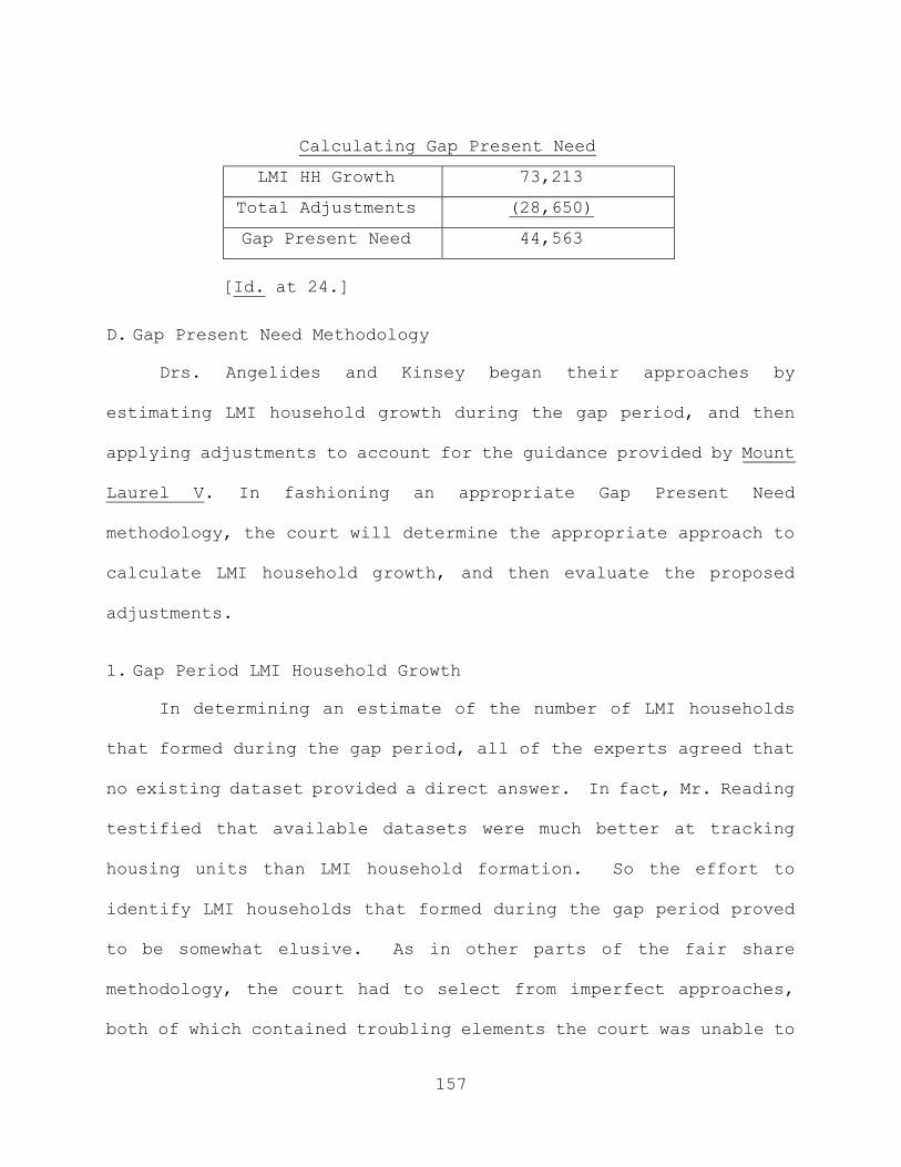
157
Calculating Gap Present Need
LMI HH Growth 73,213
Total Adjustments (28,650)
Gap Present Need 44,563
[Id. at 24.]
D. Gap Present Need Methodology
Drs. Angelides and Kinsey began their approaches by
estimating LMI household growth during the gap period, and then
applying adjustments to account for the guidance provided by Mount
Laurel V. In fashioning an appropriate Gap Present Need
methodology, the court will determine the appropriate approach to
calculate LMI household growth, and then evaluate the proposed
adjustments.
1. Gap Period LMI Household Growth
In determining an estimate of the number of LMI households
that formed during the gap period, all of the experts agreed that
no existing dataset provided a direct answer. In fact, Mr. Reading
testified that available datasets were much better at tracking
housing units than LMI household formation. So the effort to
identify LMI households that formed during the gap period proved
to be somewhat elusive. As in other parts of the fair share
methodology, the court had to select from imperfect approaches,
both of which contained troubling elements the court was unable to
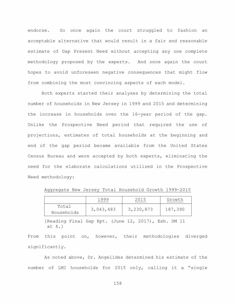
158
endorse. So once again the court struggled to fashion an
acceptable alternative that would result in a fair and reasonable
estimate of Gap Present Need without accepting any one complete
methodology proposed by the experts. And once again the court
hopes to avoid unforeseen negative consequences that might flow
from combining the most convincing aspects of each model.
Both experts started their analyses by determining the total
number of households in New Jersey in 1999 and 2015 and determining
the increase in households over the 16-year period of the gap.
Unlike the Prospective Need period that required the use of
projections, estimates of total households at the beginning and
end of the gap period became available from the United States
Census Bureau and were accepted by both experts, eliminating the
need for the elaborate calculations utilized in the Prospective
Need methodology:
Aggregate New Jersey Total Household Growth 1999-2015
[Reading Final Gap Rpt. (June 12, 2017), Exh. SM 11 at 4.]
From this point on, however, their methodologies diverged
significantly.
As noted above, Dr. Angelides determined his estimate of the
number of LMI households for 2015 only, calling it a “single
1999 2015 Growth
Total Households
3,043,483 3,230,873 187,390

159
snapshot” approach, which he deemed appropriate since the Supreme
Court combined gap need with traditional Present Need, also
calculated at a single point in time. Notably, all of his
calculations used true median incomes and not the HUD/COAH-derived
income grids endorsed by the court in Phase 1 of the trial. Dr.
Angelides calculated 2015 LMI household ratios and applied them to
total household growth during the gap period. He derived his 2015
LMI Household Ratios, by household size and region, utilizing LMI
income thresholds set at 80 percent of observed median incomes in
the 2015 ACS One-Year PUMS. Dr. Angelides then multiplied the
2015 LMI Household Ratios by the gap period Total Household Growth
for each of the 42 region and household size combinations. Dr.
Angelides asserted that this “single snapshot” approach identified
those households formed in the gap period that currently qualify
as LMI, which he then aggregated by region. Angelides Gap Rpt.
(April 12, 2017), Exh. P 86 at 20-26. He referred to his estimate
of the LMI households that formed during the gap as making up a
“pot,” from which he made deductions for various adjustments he
deemed required by Mount Laurel V. He also made certain
assumptions about each level or “strata” of LMI households derived
from true median incomes (i.e., moderate, low, and very low income
levels), which assumed that each household in the strata could
afford housing affordable to households earning the top incomes in
the category.

160
Dr. Kinsey utilized what he called a “two snapshot” approach,
whereby he determined the percentages of LMI households in 1999
and 2015 for each of 168 “cells” representing the various county
and age cohort groupings that he had also analyzed in his
Prospective Need methodology. The incomes he used in his model
were derived from COAH’s income grid from 2000 and the grid he
calculated for 2015 using HUD data because COAH had not updated
the grid itself. Using those incomes for moderate, low and very
low income households, he determined the share of total households
that were LMI for every age group by county for each of the end
points of the gap period. He then applied those LMI household
ratios in each of the cells to total households in every cell to
produce the number of LMI households at the beginning and end of
the gap period. Dr. Kinsey then subtracted the number of LMI
households in 1999 from the number in 2015, concluding that 93,398
LMI households were added during the gap period. Kinsey Gap Rpt.
(April 12, 2017), Exh. DF 85 at 28-34. Note that Dr. Kinsey later
updated this number and used 93,451 as the number of LMI households
formed during the gap period. While his calculations yielded a
statewide average of 41.16 percent of New Jersey’s households that
were qualified as LMI in 1999, using census data, and 41.66 percent
of the State’s households that were qualified as LMI in 2015, using
ACS/PUMS data, the incremental growth of LMI households during the

161
period was 49.87 percent. Reading Final Gap Rpt. (June 12, 2017),
Exh. SM 11 at 5.
Dr. Kinsey asserted —- in response to characteristics that
the Supreme Court had identified as needing to be excluded from
Gap Present Need (Mount Laurel V, 227 N.J. at 529-530) —- that the
increase in households he calculated reflected the number of LMI
households that came into existence during the gap period and were
still in existence at the end of the period. He claimed that his
model excluded those who had died and those who were income-
ineligible. Finally, Dr. Kinsey asserted that the number of LMI
households captured within traditional Present Need in 2015 should
not be subtracted from Gap Present Need despite the Supreme Court’s
explicit direction to exclude such households to avoid double-
counting because COAH had not deducted Present Need in its Prior
Cycle Prospective Need calculation, which Dr. Kinsey maintained
was the only proper way to determine Gap Present Need. See Mount
Laurel V, 227 N.J. at 529-530.
Notably, Dr. Kinsey utilized different datasets to calculate
his LMI household ratios in 1999 and in 2015, albeit out of
necessity. Reading Final Gap Rpt. (June 12, 2017), Exh. SM 11 at
4-5. Because detailed PUMS income data was not yet available in
1999, Dr. Kinsey relied on 2000 Census data, which he sorted using
the 2000 COAH income grid. Kinsey Gap Rpt. (April 12, 2017), Exh.
DF 85 at 31. Dr. Kinsey used 2000 Census income data because it

162
reflected 1999 incomes, and the 2000 COAH grid because it was
based, in part, on household income data derived from the fourth
quarter of 1999. Ibid. For 2015, Dr. Kinsey used 2015 ACS PUMS
income data. Since a COAH grid was not available for 2015, Dr.
Kinsey sorted PUMS income data using a 2015 income grid he devised
utilizing HUD 2015 county income limits, as he had done in his
Prospective Need analysis. He then applied secondary source
adjustments to his estimate of LMI households formed during the
gap period.
As in the Prospective Need phase, the approaches of the
experts yielded significantly divergent results. The difference
in their gap period LMI household growth estimates is set forth in
the following chart:
New Jersey LMI Household Growth Estimates 1999-2015
Angelides Kinsey
Total HH Growth 187,390 187,390
LMI HH Growth 73,213 93,451
LMI HH Growth Rate 39.07% 49.87%
[Reading Final Gap Rpt. (June 12, 2017), Exh. SM 11 at 5.]
For the reasons discussed below, the court prefers Dr. Kinsey’s
approach using the HUD/COAH-derived income grids to determine the
number of LMI households in 2015, but will modify his methodology
to address concerns raised by Mr. Reading about some of the results
produced by Dr. Kinsey’s model.

163
As noted above, Mr. Reading favored Dr. Angelides’ approach
because he felt it better responded to the unique circumstances
presented by the gap period and comments made by the Supreme Court
in Mount Laurel V, 221 N.J. at 529-530. For the estimation of LMI
household growth, he once again preferred Dr. Angelides’ use of
“true” mathematical medians over the COAH income grids, and
recommended this approach to the court. However, the court will
require the use of income grids in the estimation of gap period
LMI Household Growth as advocated by Dr. Kinsey and Mr. Bernard,
for the same reasons expressed above in the discussion of
Prospective Need. COAH never wavered in its use of the HUD-based
grids, and changing that policy for the gap period would lead to
a mismatch between LMI households that make up Gap Present Need
and LMI households that can qualify to live in the new deed-
restricted units ultimately made available to address this need.
In addition, although Dr. Angelides characterized his
methodology as a “single snapshot” in time in an apparent effort
to make it fit better with traditional Present Need, he started
his approach to LMI household growth by calculating the net-change
in total households during the gap period. Consequently, using
the term “single snapshot” to describe his methodology is somewhat
of a misnomer. Moreover, the Supreme Court simply did not require
that Gap Present Need mimic traditional Present Need in this or
any other way. In fact, the Court specifically noted that the
164
concept of Present Need “does not have to be limited to a survey
approach to housing units” that were substandard and would be
addressed through rehabilitation, but could and should be expanded
to include an analytical component that identifies a number of LMI
households whose need for affordable housing will be addressed by
imposing new construction obligations upon municipalities. Mount
Laurel V, 227 N.J. at 529.
Dr. Kinsey, on the other hand, stubbornly insisted that
reading Mount Laurel IV and V together required the court to follow
COAH’s Prior Cycle Prospective Need approach, even though the
Supreme Court had only acknowledged that approach “as a matter of
historical record,” and had specifically refused to endorse it or
any of the other models presented to Judge Troncone because they
had not been tested by cross-examination. See Mount Laurel V, 227
N.J. at 528, n. 7; 529. While the court favors Dr. Kinsey’s
methodology because it uses the income grids long endorsed by COAH,
the court cannot accept his inexplicably inflated Gap LMI Household
Growth Rate of almost 50 percent because of its significant
deviation from COAH’s rule of thumb. As the court noted earlier
in its discussion of Phase 1 of the trial, COAH projected constant
LMI Household Ratios throughout the Prospective Need period
because it was impossible to reliably calculate those ratios ten
years into the future due to the “many imponderables” recognized
by COAH consultant Dr. Robert Burchell. Here, however, looking
165
into the past, the court expected data to be available from which
LMI Household Ratios could be reliably estimated for both 1999 and
2015. Unfortunately, in practice this was not the case because
the data used by Dr. Kinsey at the beginning and end of the gap
period was apparently not compatible and skewed the results for
2015.
As repeated throughout this decision, COAH has consistently
observed that LMI Household Growth Rates “almost by definition”
hover around 40 percent. See, e.g., 46 N.J.R. 953 (June 3, 2014).
COAH utilized this rule of thumb because it established a range of
reasonable values around the mathematical median. Special Master
Reading thus became very troubled by Dr. Kinsey’s model that found
over 93,000 gap period households in need of affordable housing in
2015 because that calculation reflected a growth rate of 49.87
percent during the sixteen-year period. Mr. Reading characterized
this result as unreasonably high, attributing its significant
variation from COAH’s rule of thumb to the inappropriate mixing of
data sources used by Dr. Kinsey in 1999 and 2015. Indeed, Dr.
Angelides demonstrated that Dr. Kinsey’s approach produced
volatile gap period LMI Household Growth Rates between regions
from a low of five percent in Region 1, to a high of 85.1 percent
for Region 6. Exh. P 115 at 32. Even more concerning were the
variations in Dr. Kinsey’s countywide results, which were not
166
discussed in the testimony, but were admitted into evidence on CD-
ROM. Exh. DF 101 (CD-ROM):
Kinsey Countywide LMI Household Projections (sample)
County LMI HH Growth Total HH Growth LMI HH Growth
Rate Passaic 3,856 -965 -399.42%
Mercer 5,155 4,651 110.83%
Camden 3,053 530 576.46%
[Kinsey Gap Rpt., CD-ROM Tab 1c, 1d.]
Such wildly varying LMI Household Growth Rates leave many counties
far from COAH’s “about 40 percent” guidance and are indicative of
a flawed approach.
Although Mr. Reading endorsed Dr. Angelides’ approach to gap
period LMI household growth calculations, he also gave serious
consideration to Dr. Kinsey’s model as an alternative method. Mr.
Reading concluded that modifying Dr. Kinsey’s methodological steps
to apply his 2015 LMI Household Ratios, which averaged 41.66
percent statewide, to the growth in total households during the
gap period would be both “reasonable and acceptable.” Reading
Final Gap Rpt. (June 12, 2017), Exh. SM 11 at 18. Mr. Reading
testified that such modification would both negate any skewing
from data mixing, and would produce LMI Household Growth Rates
closer to the COAH benchmark of “about 40 percent.” Moreover,
using constant LMI ratios for Gap Present Need would mirror the

167
court’s handling of Dr. Kinsey’s LMI growth ratios in the
Prospective Need phase of the trial. While calculating Gap Present
Need enabled the experts to use actual data, the “imponderables”
created by the “churning” of LMI households in the gap period and
the absence of datasets to reliably measure such LMI household
formation created circumstances eerily similar to what confronted
the court when facing the projections necessary to determine
Prospective Need. Mr. Reading summarized the numerical
recommendations of the experts and added his modification of Dr.
Kinsey’s analysis in the following chart, which reflects changes
in the numbers originally used by both experts to reflect updated
total household data both experts endorsed and which was
incorporated by Mr. Reading:
New Jersey LMI Household Growth Estimates 1999-2015
Angelides Kinsey
Kinsey as modified by
Reading Total HH Growth 187,390 187,390 187,390
LMI HH Growth 73,213 93,451 78,067
LMI HH Growth Rate 39.07% 49.87% 41.66%
[Reading Final Gap Rpt. (June 12, 2017), Exh. SM 11 at 5.]
Since Dr. Kinsey’s method produced LMI Household Growth Rates
so wildly variable as to not only contradict COAH’s basic
understanding of the operation of LMI Household Ratios, but to
168
test the bounds of reasonableness, the court endorses Mr. Reading’s
modification of Dr. Kinsey’s approach. Notably, Dr. Kinsey was
never able to explain why his results were reliable despite their
significant deviation from COAH’s established rule of thumb. He
simply testified that his estimates of Gap Present Need were the
product of the calculations he performed trying to mimic COAH’s
Prior Cycle Prospective Need approach and should be accepted by
the court on that basis.
Moreover, Dr. Kinsey never convinced the court that blindly
following the Prior Cycle methodology made sense when calculating
LMI households formed during the gap period who were still in need
of affordable housing in 2015. In recalculating First Round
obligations based on over-projections, COAH appeared to be
replicating the same process it had performed in arriving at the
faulty projections, but using more recent data. See 26 N.J.R.
2348 (June 6, 1994). That makes sense when undoing a past
calculation. Notably, however, although Dr. Kinsey aimed to follow
COAH’s Prior Cycle approach, it was not clear to the court from
the rulemaking record exactly how COAH determined to reduce the
First Round obligations by a flat 48 percent. Ibid. Nor was Dr.
Kinsey able to convince the court that he knew exactly what COAH
did because the technical appendix did not contain any actual
calculations. See 26 N.J.R. 2348 (June 6, 1994). So the court was
not convinced that Dr. Kinsey’s calculations really were
169
consistent with COAH’s Prior Cycle approach. For Gap Present Need,
however, the court is not correcting a prior faulty calculation of
Prospective Need, but is looking back to estimate the number of
LMI households created over a sixteen-year period that still need
affordable housing today. That exercise strikes the court as
related to, but distinctly different from what COAH was doing to
dampen down unduly inflated obligations calculated using a
Prospective Need formula in the First Round. While aspects of
Prospective Need analysis such as use of the COAH grids seem
appropriate in determining Gap Present Need, replicating the
entire process was not a perfect fit in this context.
While the court accepts Dr. Kinsey’s assertion that
consistent data sources were not available for both 1999 and 2015,
this fact does not alter the likelihood that their use skewed his
results, causing his wildly variable gap period LMI Household
ratios and resulting in an increment in the gap period that far
exceeded COAH’s rule of thumb. Consequently, the court endorses
Special Master Reading’s analysis that Dr. Kinsey’s unacceptable
results were likely caused by inappropriate data mixing, and adopts
Mr. Reading’s modification of the Kinsey approach, which applies
Dr. Kinsey’s 2015 LMI Household Ratios to gap period total
household growth:

170
Gap Period LMI Household Growth
Total HH Growth LMI HH Growth
Region Four 40,625 17,324
New Jersey 187,390 77,677
Mr. Reading’s modification actually produces a statewide average
LMI Household Growth Rate of 41.45 percent, which is slightly lower
than the 41.66 percent average of the applied 2015 LMI Household
Ratios, due to household growth distributions.
Although the court recognizes that LMI Household Growth
Rates can fluctuate around 40 percent, and are not completely
static, the court viewed its choice here as being between applying
Dr. Kinsey’s 2015 ratios to total household growth, which produces
a statewide average LMI Household Growth Rate of 41.45 percent, or
using his incremental approach that yielded an average growth rate
of 49.87 percent. Faced with these alternatives, the court deemed
it better, and ultimately more reasonable, to apply the 2015 LMI
Household Ratios to diminish the wildly divergent county and
individual “cell” ratios calculated by Dr. Kinsey.
Having decided to incorporate this modification of Dr.
Kinsey’s approach into the fair share methodology, the court now
considers the very different adjustments proposed by Dr. Angelides
and Dr. Kinsey in their calculations of the gap period affordable
housing need that remained unmet in 2015. Since the methodological
171
steps of the experts do not match, the court will consider each
expert’s adjustments separately.
2. Dr. Kinsey’s Adjustments
Dr. Kinsey adjusted Gap Present Need by adapting his entire
Prospective Need methodology to the Gap Period. As noted above,
Dr. Kinsey’s approach is largely based on his understanding of
COAH’s 1994 Prior-Cycle Prospective Need recalculation, using the
“most up-to-date available data that reflected actual, observed
growth during the gap period.” Kinsey Gap Rpt. (April 12, 2017),
Exh. DF 85 at 10.
a. Reallocation of Working Age Household Growth
In keeping with his Prospective Need methodology, the first
adjustment to gap period LMI household growth that Dr. Kinsey
proposed was to pool and reallocate portions of that growth
occurring in households below age 65 to regions based on historic
job growth. Id. at 33. This reallocation of working age household
growth was included by COAH as part of the Second Round Prospective
Need calculations:
. . . the growth of households below age 65 is put into a statewide pool and allocated to regions of the state according to the proportional share of nonresidential ratable growth... Thus, growth in the working-age component of low- and moderate-income households was assigned to regions where jobs previously grew. On the other hand, growth in

172
the elderly and presumably non-working population was retained in the original region where this growth took place.
[26 N.J.R. 2347 (June 6, 1994).]
However, this pooling and reallocation step was not applied in the
calculation of Prospective Need in this trial because neither Dr.
Kinsey nor Dr. Angelides attributed any of the LMI household growth
during the Prospective Need period to households headed by persons
younger than 65 years of age, reflecting the demographic
characteristics of the Baby Boomer generation. See Reading Rpt.
(August 31, 2016), Exh. SM 4 at 50. Moreover, there is no
indication in the rulemaking record whether COAH included a
reallocation of need in its Prior Cycle Prospective Need
calculation. See 26 N.J.R. 2348 (June 6, 1994).
Mr. Bernard agreed with Dr. Kinsey’s inclusion of this step
to determine Gap Present Need as it would counter the displacement
of LMI households from areas of job growth that occurred during
the gap period. Mr. Reading questioned including this inter-
regional reallocation step, however, because its purpose in Prior
Rounds was to predict areas of future housing need based on
previous employment growth and not on the housing need of LMI
households that already exist. Reading Final Gap Rpt. (June 12,
2017), Exh. SM 11 at 5-6. Mr. Bernard countered that although the
LMI households already existed, the affordable housing units to
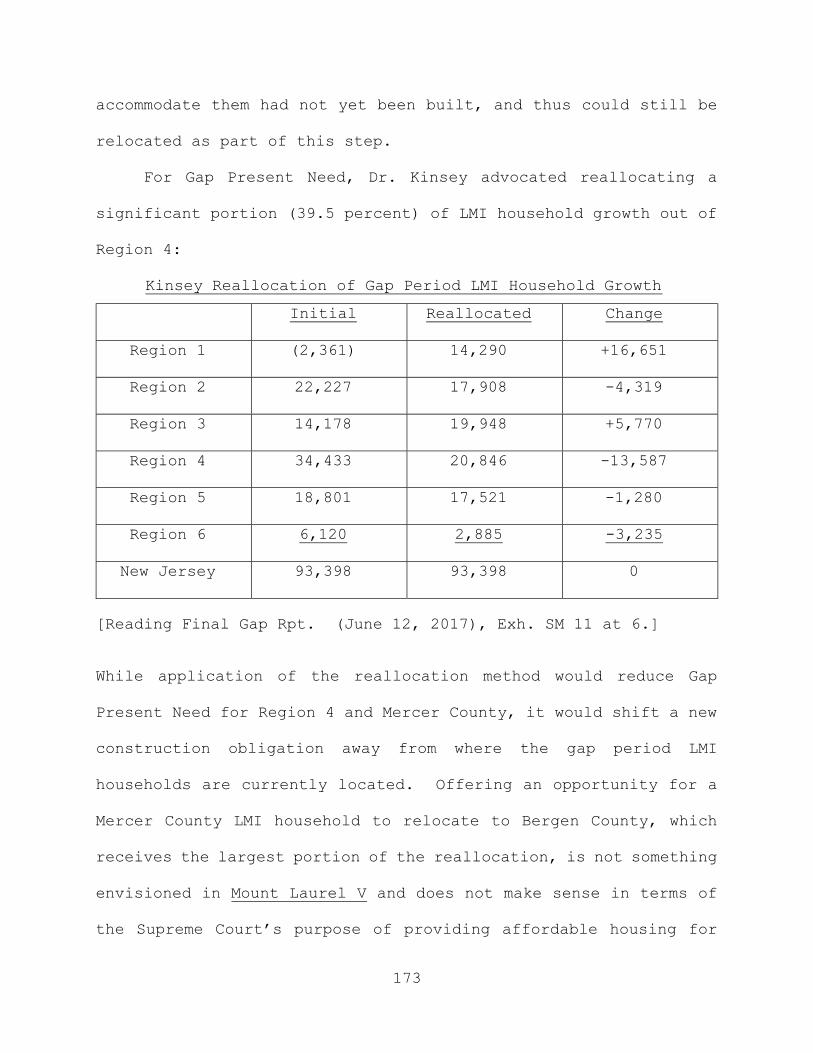
173
accommodate them had not yet been built, and thus could still be
relocated as part of this step.
For Gap Present Need, Dr. Kinsey advocated reallocating a
significant portion (39.5 percent) of LMI household growth out of
Region 4:
Kinsey Reallocation of Gap Period LMI Household Growth
Initial Reallocated Change
Region 1 (2,361) 14,290 +16,651
Region 2 22,227 17,908 -4,319
Region 3 14,178 19,948 +5,770
Region 4 34,433 20,846 -13,587
Region 5 18,801 17,521 -1,280
Region 6 6,120 2,885 -3,235
New Jersey 93,398 93,398 0
[Reading Final Gap Rpt. (June 12, 2017), Exh. SM 11 at 6.]
While application of the reallocation method would reduce Gap
Present Need for Region 4 and Mercer County, it would shift a new
construction obligation away from where the gap period LMI
households are currently located. Offering an opportunity for a
Mercer County LMI household to relocate to Bergen County, which
receives the largest portion of the reallocation, is not something
envisioned in Mount Laurel V and does not make sense in terms of
the Supreme Court’s purpose of providing affordable housing for
174
presently existing LMI households formed during the gap period.
This court has been focused on determining the current need of Gap
Period LMI Households in Mercer County and establishing municipal
obligations to meet that need. Incorporating this step into a
calculation of Gap Present Need is an example of how blindly
following the Prospective Need methodology is not a good fit to
satisfy the task assigned to the court. Consequently, the court
rejects Dr. Kinsey’s proposed reallocation of LMI household growth
between regions, which would shift a significant percent of need
away from where LMI gap households are living today.
b. Gap Period Secondary Source Adjustments
After reallocating gap period LMI household growth between
regions, Dr. Kinsey’s next adjustment was for municipal secondary
sources. Dr. Kinsey’s approach was a further adaptation of his
fair share Prospective Need methodology, including allocating
regional Gap Present Need to the municipalities in each region,
then calculating and applying municipal secondary source
adjustments, but retrospectively for the gap period. Reading Final
Gap Rpt. (June 12, 2017), Exh. SM 11 at 19. As in his Prospective
Need methodology, Dr. Kinsey adjusted municipal Gap Present Need
to reflect estimated changes in the housing stock attributable to
demolitions, conversions and filtering. Ibid. Dr. Kinsey’s gap
period secondary source adjustments increased statewide Gap
Present Need significantly:

175
Kinsey New Jersey Gap Period Secondary Source Adjustments
Demolitions 37,050
Filtering 44,263
Conversions 15,408
Less Urban Aid (40,347)
Secondary Sources 56,374
[Reading Final Gap Report (June 12, 2017), SM 11 at 8.]
Special Master Reading recommended rejecting Dr. Kinsey’s Gap
Present Need secondary source adjustments, concluding that because
such adjustments were conceived as predictive calculations, they
should apply only as part of a future Prospective Need methodology.
As observed by Dr. Kinsey, however, COAH included secondary source
adjustments in its calculation of Prior Cycle Prospective Need,
which was a retrospective calculation. 26 N.J.R. 2348 (June 6,
1994). As the court noted above, however, in the Second Round
COAH was retro-fitting its Prospective Need calculations from the
First Round in order to reduce the obligations it had previously
over-projected, and may have included secondary source adjustments
because they had been incorporated into the formula applied in the
First Round to establish the obligations COAH was then revising.
Mr. Reading expressed additional concern that Dr. Kinsey’s
proposed adjustments had the potential to double count demolitions
and conversions, which had already occurred and may have been
included to some extent in calculating traditional Present Need.
176
Although Mr. Bernard generally agreed with Dr. Kinsey’s use of
demolitions and conversions to expand Gap Present Need, he joined
Mr. Reading in expressing discomfort with the inclusion of
filtering in the calculation of that need for the same reasons
they both rejected filtering previously in the calculation of
Prospective Need. Mr. Bernard also took exception to how Dr.
Kinsey calculated conversions and handled the Highlands area of
the State.
The court is wary about adjusting Gap Present Need to add
secondary sources. The Supreme Court in Mount Laurel V focused on
LMI households created during the gap. When estimating households
that have already formed, making adjustments for changes in housing
units such as those caused by demolitions and conversions that
have already occurred seems incompatible with the task at hand.
That Dr. Kinsey’s Gap Present Need soared far above the number of
Gap Period LMI Households he identified as having been formed
during the gap period underscored yet again how a full Prospective
Need approach is incompatible with the thrust of the Supreme
Court’s gap period analysis.
Indeed, Dr. Kinsey’s use of secondary sources focuses on
housing units and not households, fundamentally remaining at odds
with this court’s conception of the components necessary to
calculate Gap Present Need. Firstly, adding significantly to the
gap need due to filtering is as ill-advised in this context due to
177
the unproven complexities of the model designed by Dr. Kinsey as
it was when the court considered a similar adjustment for
Prospective Need. Notably, Mr. Bernard recommended rejecting this
adjustment in both Phases 1 and 2 of the trial, a recommendation
concurred in by Mr. Reading. The court agrees that there is no
place in a “fair estimate” of Gap Present Need for an adjustment
based on filtering. The proposed method is simply too unreliable
to be incorporated into a calculation of Gap Present Need.
While excluding demolitions and conversions is not as clear
cut, they do not have a viable place in a retrospective analysis
based on the need of Gap Period LMI Households for affordable
housing in 2015 when those changes in the housing market have
already occurred. This court is not undoing a past over-projection
calculated with data shown in retrospect to be faulty, and retro-
fitting a similar analysis to arrive at a reduction in prior
obligations. Moreover, adding conversions and demolitions as
calculated by Dr. Kinsey again significantly inflates Gap Present
Need above the number of gap period LMI households he asserts was
created during the period. As noted above, such a result makes no
sense to the court. To the extent Dr. Kinsey made these
adjustments as a way to address the circumstances he described
concerning cost-burdened LMI households that formed during the
gap, Dr. Kinsey and Mr. Bernard admitted that COAH had never
included this consideration in any of its fair share housing

178
models, largely due to the complexities and imponderables such
consideration would entail. Finally, the court simply lacks
confidence that such adjustments make sense in the context of Gap
Present Need. Should similar circumstances arise in the future,
the court hopes a reconstituted agency will be available to
evaluate important policy considerations underlying the necessary
retrospective analysis. For present purposes, however, the court
rejects secondary source adjustments when calculating Gap Present
Need.
3. Dr. Angelides’ Adjustments
Dr. Angelides responded creatively to the concerns expressed
by the Supreme Court in Mount Laurel V and fashioned three novel
adjustments for the court’s consideration. While the court was at
first attracted by Dr. Angelides’ adjustments as facially
responsive to the Supreme Court’s comments concerning the
characteristics of Gap Present Need, 227 N.J. at 526-531, closer
scrutiny caused the court to lose confidence in many aspects of
the reductions in Present Need that he advocated. Although the
court does not adopt his proposals to reduce Gap Present Need for
Gap Period LMI Households that found affordable housing or Gap
Period LMI Households with significant housing assets, the court
did find his adjustment for traditional Present Need overlap to be
valid as modified.
179
a. LMI households living in affordable housing
The first adjustment undertaken by Dr. Angelides to translate
Gap Period LMI household growth into Gap Present Need was to
exclude those LMI households, formed during the gap period, that
were living “in a housing unit affordable to their income strata
(as defined in the Fair Housing Act) in 2015, provided the
household is not overcrowded within the unit (as defined in COAH’s
Present Need standard).” Angelides Gap Rpt. (April 12, 2017), Exh.
P 86 at 28. However, because there was no data source that
specifically identified which 2015 LMI households were formed
during the gap period, Dr. Angelides made his estimation by
assuming that the same proportion of 2015 Gap Period LMI Households
would be in affordable units as was the case for all 2015 LMI
households in affordable housing. Id. at 29, n.34.
Dr. Angelides utilized 2015 ACS PUMS data to categorize each
LMI household by its income status “strata” (moderate, low, or
very low-income) and then compared the households in each strata
with the affordability of the unit in which they were residing to
determine those LMI households that were living in affordable
housing in 2015. Id. at 29-30. Dr. Angelides then removed those
households living in overcrowded units, as defined in traditional
Present Need methodology, to avoid double counting. Id. at 30-31.
From these calculations, Dr. Angelides next determined the
proportion of all 2015 LMI households in each region and household
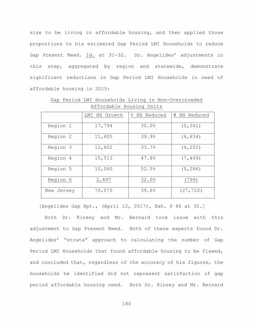
180
size to be living in affordable housing, and then applied those
proportions to his estimated Gap Period LMI Households to reduce
Gap Present Need. Id. at 31-32. Dr. Angelides’ adjustments in
this step, aggregated by region and statewide, demonstrate
significant reductions in Gap Period LMI Households in need of
affordable housing in 2015:
Gap Period LMI Households Living in Non-Overcrowded Affordable Housing Units
LMI HH Growth % HH Reduced # HH Reduced
Region 1 17,794 30.0% (5,341)
Region 2 11,605 39.9% (4,634)
Region 3 12,602 33.7% (4,252)
Region 4 15,513 47.8% (7,409)
Region 5 10,060 52.5% (5,286)
Region 6 2,497 32.0% (799)
New Jersey 70,070 39.6% (27,720)
[Angelides Gap Rpt., (April 12, 2017), Exh. P 86 at 32.]
Both Dr. Kinsey and Mr. Bernard took issue with this
adjustment to Gap Present Need. Both of these experts found Dr.
Angelides’ “strata” approach to calculating the number of Gap
Period LMI Households that found affordable housing to be flawed,
and concluded that, regardless of the accuracy of his figures, the
households he identified did not represent satisfaction of gap
period affordable housing need. Both Dr. Kinsey and Mr. Bernard

181
testified that Dr. Angelides overstated the households living in
affordable housing because he compared each LMI household’s actual
housing costs to the maximum affordable housing costs for
households at the highest qualifying LMI income, rather than to
the maximum housing costs based on each household’s actual income.
When Dr. Kinsey reportedly reproduced Dr. Angelides’ approach in
this step, but determined affordability based on each household’s
actual income, total LMI households living in affordable housing
were less than half the number calculated by Dr. Angelides. Exh.
DF 95a at 1.
Dr. Kinsey and Mr. Bernard further challenged the accuracy of
Dr. Angelides’ calculations, specifically questioning the manner
in which he estimated the number of Gap Period LMI Households in
affordable housing by applying the proportions of total Gap Period
LMI Households in affordable housing to gap period LMI household
growth. Both experts asserted that the application of these
proportions was based on the faulty assumption that newly
established Gap Period LMI Households would be able to find
affordable housing at the same rate as already established LMI
households. Mr. Bernard considered this assumption to be
counterintuitive given the diminishing affordable housing choices
available during the gap period, which included the Great
Recession. In addition, Dr. Kinsey pointed out that Dr. Angelides
mixed income requirements in a novel and troubling way, utilizing
182
true median incomes for his calculations that have been rejected
by the court, but also introducing consideration of HUD standards
he had spurned in other instances in his methodology and accepting
only portions of UHAC regulations. Dr. Kinsey characterized the
process as using a “hodge-podge affordability definition . . .
that mixes and matches different standards and definitions.”
Kinsey Response Gap Rpt. (April 24, 2017), Exh. DF 86 at 17. Dr.
Kinsey asserted that such mixing was inherently unreliable.
In the strata approach Dr. Angelides used to reduce Gap
Present Need, he essentially sorted LMI households living in cost-
burdened housing in 2015 from those households that were not cost-
burdened. Mr. Bernard questioned the results of this method to
reduce need, citing census-based HUD data to show an increase in
cost-burdened households in New Jersey during the gap period.
Cost-burdened households are those that spend over a set percentage
of their incomes for housing, ranging from 28 percent to over 30
percent. Mr. Bernard’s data showed that there was a total increase
in cost-burdened households from about 61 percent to 75 percent
during the gap period, and that the increase in LMI households
that were cost-burdened between 2000 and 2010 was more than three
times the number of LMI households created during the gap. Exh. DB
47. Mr. Bernard testified that these figures showed a significant
loss of affordable housing over the gap period, most of which he
attributed to gentrification. As a result of these circumstances,
183
Mr. Bernard asserted that, while some LMI households did find
affordable housing during the gap period, far more LMI households
lost affordable housing as their incomes declined. Mr. Bernard
therefore concluded that any Gap Period LMI Households that found
affordable housing did not represent a satisfaction of “pent-up
affordable housing need,” pursuant to Mount Laurel V, and should
therefore not be used to reduce Gap Present Need.
Both Dr. Kinsey and Mr. Bernard further criticized the
reduction in Gap Present Need for Gap Period LMI Households that
found deed-restricted affordable housing during the period as
being redundant. While the adjustment made by Dr. Angelides
included Gap Period LMI households in both deed restricted and
non-deed-restricted units, reductions in municipal obligations for
creation of deed-restricted affordable housing are applied as
credits during the compliance process. Therefore, to avoid double
counting, both Dr. Kinsey and Mr. Bernard recommended that if any
municipal housing obligations were to be reduced for gap period
LMI households that found deed-restricted affordable housing, such
deductions should only be accomplished through municipal bonus
credits awarded during the compliance process.
Special Master Reading endorsed Dr. Angelides’ adjustment,
concluding that his approach was well-reasoned and supported by
available data sources. Mr. Reading responded to Mr. Bernard’s
concern regarding increases in New Jersey’s cost-burdened

184
households during the gap period by noting that Judge Serpentelli
in AMG, 207 N.J. Super. at 422-423, had rejected incorporating
cost—burdened households in the calculation of Present Need, and
COAH and other courts had agreed with this conclusion. Mr. Reading
did, however, concur with the criticisms expressed by Dr. Kinsey
and Mr. Bernard regarding the exclusion of LMI households living
in deed-restricted affordable housing because to include them
would be redundant since municipalities receive credits for those
units toward satisfaction of their fair share obligations during
the compliance process. Excluding deed-restricted units would
prevent double counting those units. Reading Final Gap Rpt., (June
12, 2017), Exh. SM 11 at 20. As a result, Mr. Reading proposed
that the 2,368 LMI households he calculated as living in deed-
restricted affordable housing remain included in Gap Present Need
to avoid the possibility of double counting. Id. at 24:
Gap Period LMI Households Living in Non-Overcrowded, Non-Deed
Restricted Affordable Housing Units (Reading)
New Jersey 28,963
Less Deed Restricted (2,368)
Total 26,595
[Reading Final Gap Rpt. (June 12, 2017), Exh. SM 11 at 24.]
The court concurs with Special Master Reading that COAH
rejected consideration of cost-burdened households in calculating
municipal affordable housing obligations, and that its decision

185
was upheld by the Appellate Division as a permissible exercise of
discretion. In Re Adoption of N.J.A.C. 5:94 and 5:95, 390 N.J.
Super. at 36. Such considerations cannot drive the calculation of
Gap Present Need despite the challenging circumstances experienced
by such LMI households that formed during the gap period. Further,
while the court appreciates Dr. Angelides’ effort to restrict Gap
Present Need to those households “still in need of affordable
housing” in response to language used by the Supreme Court in Mount
Laurel V, 227 N.J. at 528-531, the court is not convinced that
those households identified by Dr. Angelides in this step reliably
represent a reduction in gap period need. The court was troubled
by the compelling criticisms of Dr. Kinsey and Mr. Bernard, which
were based on statistical evidence they provided that called the
deductions taken by Dr. Angelides into question. Moreover,
reductions in Gap Present Need based on an analysis of cost-
burdened households, as this adjustment appeared to be, are at
odds with COAH and judicial precedent rejecting such
considerations in prior methodologies. The court also remained
unconvinced that the strata approach utilized by Dr. Angelides was
reliable, especially as it was not based on the COAH income grid
and mixed affordability criteria.
In Mount Laurel IV, the Supreme Court specifically identified
COAH’s exclusion of cost-burdened households from Present Need
calculations as having been judicially approved and among the
186
policies for trial courts to follow in fashioning their fair share
methodologies:
[I]n addressing the first iteration of Third Round Rules, the Appellate Division also approved the "exclu[sion of] the cost-burdened poor from the present need or rehabilitation share calculation." In doing so, the appellate panel noted that pre-FHA courts also had allowed exclusion of the "cost-burdened poor" from the fair share formula. The court found that COAH's decision to exclude the cost-burdened poor was a permissible exercise of discretion.
Mount Laurel IV, 221 N.J. at 32-33 (citations omitted).]
COAH’s Prior Round rules largely adopted the approach developed in
AMG, 207 N.J. Super. at 422-423, which excluded consideration of
cost-burdened households from the calculation of Present Need.
The Appellate Division concurred with this conclusion in In re
Adoption of N.J.A.C. 5:94 & 5:95, 390 N.J. Super. at 23, 35, which
justified the exclusion primarily on the difficulty of accurately
calculating the number of cost-burdened households. Drawing
largely from Judge Serpentelli’s analysis, the appellate court
reasoned as follows:
First, many people do not fully report their income. Second, some people, by choice, pay "a disproportionate amount of their income for housing." Third, some people choose lesser quality housing than they can afford, thereby creating a housing "mismatch." If household unit income and housing unit cost were more closely correlated, more units would be available for needy families. Fourth, many retirees who have lower incomes nonetheless have substantial assets. Fifth, the needs of
187
lower income households could be met more appropriately through income maintenance programs rather than revision of land use regulations. Sixth, many of the cost-burdened poor also occupy substandard units, thereby creating a duplication in the present need count.
[In re Adoption of N.J.A.C. 5:94 & 5:95, 390 N.J. Super. at 35 (citations omitted).]
See also 36 N.J.R. 5798, 5809-5810 (December 20, 2004), where COAH
specifically addressed the exclusion when it provided additional
policy-based justifications as part of the notice and comment
process.
In using cost-burdened concepts to exclude Gap Period LMI
Households from Gap Present Need, Dr. Angelides thus ventured into
territory COAH had assiduously avoided. And in criticizing his
adjustment, Dr. Kinsey and Mr. Bernard also made arguments based
on cost-burdened concepts. Without guidance from COAH and the
appellate courts as to how such concepts might appropriately be
incorporated into any calculation of municipal obligations, this
court is unwilling to endorse an approach based on an analysis of
cost-burdened households, especially one where the testimony of
the experts was so sharply conflicting. Indeed, Dr. Angelides’
adjustment is susceptible to all of the potential inaccuracies
connected with a cost-burdened analysis highlighted in AMG, and
the appellate cases that concurred in Judge Serpentelli’s
reasoning.

188
Although Gap Present Need is a new addition to the fair
share methodology, the court remained skeptical that cost-burdened
concepts could be incorporated into determining a “fair estimate”
of that Need. The bottom line is that the adjustment as structured
by Dr. Angelides is simply too unreliable to be accepted by the
court to significantly dilute Gap Present Need. Accepting this
adjustment would run afoul of well-established COAH precedent
based on the inherent lack of reliability in such an analysis.
Furthermore, other aspects of Dr. Angelides’ approach raise
even more questions about his calculations. First, to estimate
the number of LMI households in affordable housing that formed
during the gap period, Dr. Angelides assumed that the proportion
of those Gap Period LMI Households that found affordable housing
would be the same as the proportion of all 2015 LMI households in
affordable housing. While this approach may appear reasonable at
first glance, it assumes that Gap Period LMI Households were able
to acquire affordable housing during the gap period at the same
rate as all LMI households. The court, however, shares the
concerns raised by Mr. Bernard that it is counterintuitive to
assume that the relatively new LMI households formed during the
gap period would have the same level of access to affordable
housing opportunities as those LMI households established before
1999. Those households in LMI status for longer periods of time
would likely be more familiar with the processes to find and

189
qualify for affordable housing, and may already have been living
in affordable units for considerable periods of time. To the
extent that some percentage of LMI households are living in owner-
occupied residences, the ability of newer formed LMI households to
purchase property would likely not match their more established
counterparts. These concerns cause the court to further doubt the
reliability of Dr. Angelides’ proposed adjustment.
Second, although Mr. Reading found Dr. Angelides’ overall
approach to be reasonable, the court is concerned with his use of
“strata” to determine housing affordability. The court agrees
with Dr. Kinsey and Mr. Bernard that setting housing affordability
thresholds from the maximum incomes for each strata, rather than
using the actual incomes of each household, tends to inflate the
number of households in affordable housing. Dr. Angelides’ strata
approach is especially puzzling considering that PUMS data can be
used to compare each household’s actual income to the cost of the
housing they occupy. In addition, Dr. Kinsey and Mr. Bernard
presented further credible evidence to make the court question the
propriety of Dr. Angelides’ mixing and matching of income standards
from the UHAC, HUD, and his own methodology based on true medians,
raising the distinct possibility that his estimate of Gap Period
LMI Households living in affordable housing was significantly
inflated. Exh. DF 86 at 16.
190
The court also had serious misgivings about the proposed
adjustment due to the likely negative ramifications of Dr.
Angelides’ reductions on the fair share municipal compliance
process. Notably, Dr. Angelides reiterated often during the trial
that he had no expertise in the process through which towns design
and adopt fair share plans to comply with their affordable housing
obligations. So it was not surprising that he did not appear to
realize or to be concerned about the likely impact on the
compliance process of his proposed adjustment that removed from
Gap Present Need those Gap Period LMI Households living in deed-
restricted units.
When developing fair share plans to respond to the identified
affordable housing need, municipalities can obtain credits toward
their affordable housing obligations from the creation of deed-
restricted affordable housing units. COAH relied upon a well-
established system of “bonus credits” in the compliance process to
incentivize towns to take various actions such as approving
inclusionary developments, constructing affordable housing units
for very-low income households, making family rental units
available, or providing affordable units in designated
redevelopment or rehabilitation areas. See, e.g., Mount Laurel IV,
221 N.J. at 31-32.
The court agrees with Mr. Bernard and Mr. Reading that Dr.
Angelides’ adjustment could very well result in deed-restricted
191
housing being counted twice toward the satisfaction of a town’s
obligation, and thus improperly diluting the need. To avoid this
double counting would require the modification of the compliance
process, which in turn would deprive municipalities of credits for
deed-restricted housing constructed during the gap period and now
occupied by Gap Period LMI Households. Such a modification would
also benefit municipalities that did not actually build affordable
housing units during the gap by reducing their Gap Present Need
obligations. Adopting this approach would interfere with COAH’s
well-established compliance process and thwart the reasonable
expectations of municipalities that have been relying on credits
in developing their Third Round fair share plans through
settlements, many of which have already been approved throughout
New Jersey, including several by this court.
Perhaps most importantly, however, is that disallowing
credits for towns where affordable housing was developed in the
gap period would undermine the special treatment accorded to them
by the Supreme Court in Mount Laurel IV, 221 N.J. at 21-27; see
also Mount Laurel V, 227 N.J. at 523-525 (describing the rationale
behind “the Court’s different, and better, treatment of towns that
had already started taking meaningful steps toward compliance
during [the gap] period,” and thus had “willingly accepted
responsibility for the need arising while COAH worked to adopt
controlling rules for that very time period and going forward.”).
192
Such a result cannot be countenanced. To avoid double-counting
and to preserve the well-established expectations of
municipalities engaged in the compliance process thus constitute
yet additional reasons for the court to reject Dr. Angelides’
proposed removal from Gap Present Need of LMI gap households that
found deed-restricted affordable housing between 1999 and 2015.
While deed-restricted housing was only a subset of the proposed
adjustment, the negative effect of this adjustment on the
compliance process further erodes the court’s confidence in the
methodology advocated by Dr. Angelides. In short, the court
rejects the adjustment to remove gap households living in
affordable housing from Gap Present Need because it is too
unreliable and threatens to significantly and inappropriately
dilute municipal new construction obligations for the gap period.
b. LMI Households with Significant Housing Assets
For his second adjustment, Dr. Angelides reprised the
significant asset test from his Prospective Need calculations.
Reading Final Gap Rpt. (June 12, 2017), Exh. SM 11 at 12. Utilizing
2015 ACS PUMS data, Dr. Angelides excluded those LMI households
that owned their own homes with no mortgage, had total housing
costs of less than 38 percent of their income, and their primary
residence had a value in excess of the regional asset limit
published by COAH. Mr. Reading recorded the results of this
adjustment in his report to the court:
193
Gap Period LMI Households with Significant Assets
LMI HH Growth(adj.)
# HH Excluded % HH Excluded
New Jersey 42,351 (1,958) -4.6%
Region 4 8,104 (314) -3.9%
[Id. at 13.]
The court reiterates its rejection of a significant asset
test for the same reasons expressed in the Prospective Need
analysis and agrees with Special Master Reading that such a test
should be included only as part of a comprehensive re-evaluation
of the entire fair share methodology by COAH, and not adopted as
an isolated policy that would reduce affordable housing need
without considering off-setting factors. While the test is a
reasonable one, COAH only considered adding it to the methodology
in the various iterations of the Third Round when it also adopted
changes that somewhat balanced the reductions in need anticipated
from the asset test with new requirements that would increase the
overall need. This issue thus remains one better left to the
Executive and Legislative branches, hopefully to be addressed in
the future by a reconstituted and functioning COAH.
c. Overlap with Traditional Present Need
Dr. Angelides’ third and final adjustment before allocating
regional Gap Present Need to the municipalities was to remove those
Gap Period LMI Households already included in traditional Present
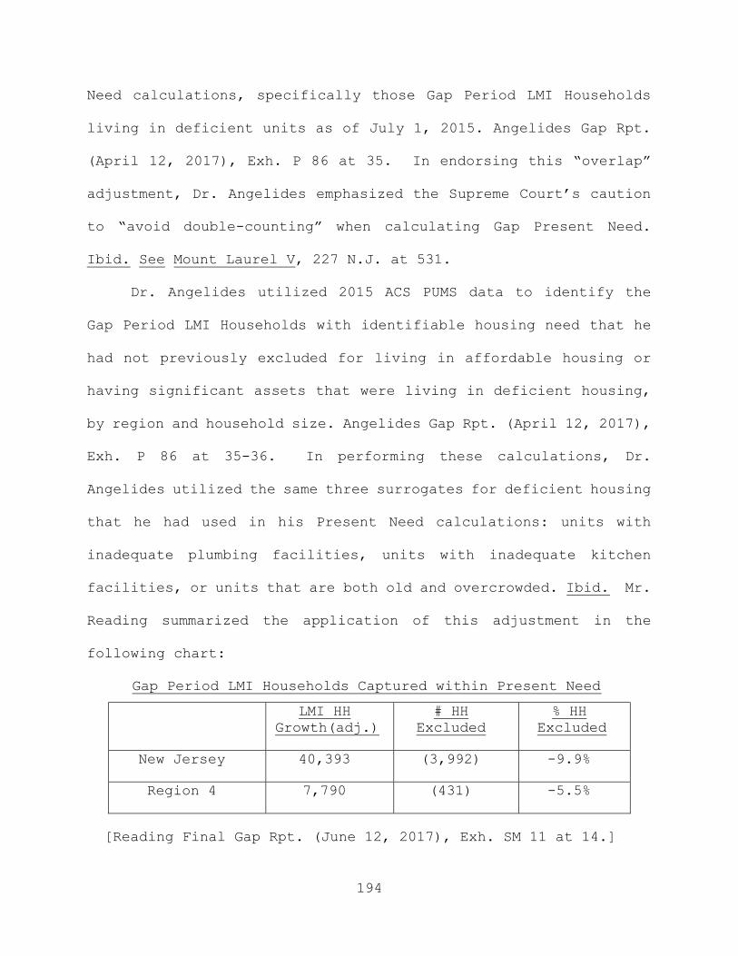
194
Need calculations, specifically those Gap Period LMI Households
living in deficient units as of July 1, 2015. Angelides Gap Rpt.
(April 12, 2017), Exh. P 86 at 35. In endorsing this “overlap”
adjustment, Dr. Angelides emphasized the Supreme Court’s caution
to “avoid double-counting” when calculating Gap Present Need.
Ibid. See Mount Laurel V, 227 N.J. at 531.
Dr. Angelides utilized 2015 ACS PUMS data to identify the
Gap Period LMI Households with identifiable housing need that he
had not previously excluded for living in affordable housing or
having significant assets that were living in deficient housing,
by region and household size. Angelides Gap Rpt. (April 12, 2017),
Exh. P 86 at 35-36. In performing these calculations, Dr.
Angelides utilized the same three surrogates for deficient housing
that he had used in his Present Need calculations: units with
inadequate plumbing facilities, units with inadequate kitchen
facilities, or units that are both old and overcrowded. Ibid. Mr.
Reading summarized the application of this adjustment in the
following chart:
Gap Period LMI Households Captured within Present Need
LMI HH Growth(adj.)
# HH Excluded
% HH Excluded
New Jersey 40,393 (3,992) -9.9%
Region 4 7,790 (431) -5.5%
[Reading Final Gap Rpt. (June 12, 2017), Exh. SM 11 at 14.]

195
After initially rejecting this adjustment, Mr. Bernard
testified that a step addressing the overlap between traditional
Present Need and Gap Present Need could have merit. But Mr.
Bernard recommended that Dr. Angelides’ adjustment be modified to
not remove the 62 percent of Gap Period LMI Households in deficient
housing located in QUAMs because including them would not result
in double counting since urban aid municipalities do not have a
new construction obligation. Mr. Bernard reasoned that, without
a new construction obligation, QUAMs would not receive both a
traditional Present Need rehabilitation obligation and a Gap
Present Need new construction obligation for the same LMI
Household. According to Mr. Bernard’s interpretation of Mount
Laurel V, a prohibited overlap occurs only when redundant
traditional Present Need and Gap Present Need obligations are
allocated to the same municipality. However, Mr. Bernard
acknowledged that excluding QUAMs from this adjustment, as he
proposed, could theoretically result in a deficient unit being
rehabilitated in a QUAM and a new unit being built elsewhere in
the region for the same Gap Period LMI Household.
Special Master Reading concluded that Dr. Angelides’
traditional Present Need overlap calculation represented a
reasonable and necessary adjustment to Gap Present Need, and was
explicitly contemplated by the Supreme Court in Mount Laurel V.
Reading Final Gap Rpt. (June 12, 2017), Exh. SM 11 at 22. Mr.
196
Reading also agreed with Mr. Bernard’s recommendation that
traditional Present Need in QUAMs not be removed from the
calculation of Gap Present Need because these municipalities do
not receive allocations of Gap Present Need. Ibid. Mr. Reading
estimated that 61.80 percent of statewide and 28.30 percent of
Region 4 traditional Present Need was located in QUAMs. Mr.
Reading recommended excluding these percentages from the
adjustment, resulting in a decrease in Dr. Angelides’ overlap of
2,055 units. Id. at 22-24.
The court concurs with the recommendations of Mr. Bernard and
Mr. Reading to modify Dr. Angelides’ adjustment to remove the
deduction for Present Need in QUAMs. First, the court’s focus in
Gap Present Need is in determining a new construction obligation
for Princeton and West Windsor. Since their respective traditional
Present Needs will be deducted from their Gap Present Need
obligations, those towns will be not be responsible to rehabilitate
a unit and also provide a unit of new construction for the same
Gap LMI household. That is the overlap that concerned the Supreme
Court, which was examining a new construction obligation when it
created Gap Present Need. Since QUAMs do not have any new
construction need, the Supreme Court did not discuss their special
status in Mount Laurel V, nor did the Court mention urban aid
municipalities at all when identifying the overlap with
traditional Present Need that trial courts should avoid. Mount

197
Laurel V, 227 N.J. at 531. If Gap Period LMI households in
deficient housing are excluded from Mercer County’s new
construction obligation, those households may be deprived of an
opportunity to access affordable housing in the region outside of
Trenton. That result seems at odds with the intent of the Supreme
Court in Mount Laurel V. Moreover, COAH itself recognized that
excess Present Need should be reallocated out of urban areas that
had higher than average substandard units. N.J.A.C. 5:93-2.4;
N.J.A.C. 5:93-2.5; 26 N.J.R. 2346-2347 (June 6, 1994). Reducing
the adjustment for overlap with Present Need to remove the Present
Need in QUAMs strikes the court as consistent with the policies
underlying COAH’s regulations providing for the reallocation of
Present Need from urban areas with large amounts of deficient
housing to other municipalities.
The court agrees with Special Master Reading that Dr.
Angelides has submitted a reasonable approach for the Present Need
overlap adjustment, to be modified to exclude the Present Need in
QUAMs. Since Dr. Angelides incorporated the adjustment for
traditional Present Need as part of a sequence that relied upon
his first two adjustments that the court has rejected, the court
directed Mr. Reading to apply the Present Need adjustment, minus
Present Need in QUAMs. As modified, the results of the adjustment
are reflected in the following chart:
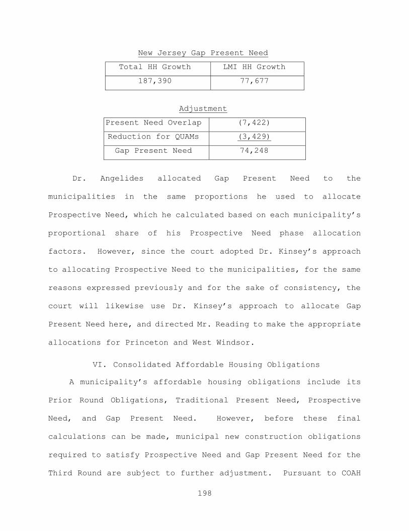
198
New Jersey Gap Present Need
Total HH Growth LMI HH Growth
187,390 77,677
Adjustment
Present Need Overlap (7,422)
Reduction for QUAMs (3,429)
Gap Present Need 74,248
Dr. Angelides allocated Gap Present Need to the
municipalities in the same proportions he used to allocate
Prospective Need, which he calculated based on each municipality’s
proportional share of his Prospective Need phase allocation
factors. However, since the court adopted Dr. Kinsey’s approach
to allocating Prospective Need to the municipalities, for the same
reasons expressed previously and for the sake of consistency, the
court will likewise use Dr. Kinsey’s approach to allocate Gap
Present Need here, and directed Mr. Reading to make the appropriate
allocations for Princeton and West Windsor.
VI. Consolidated Affordable Housing Obligations
A municipality’s affordable housing obligations include its
Prior Round Obligations, Traditional Present Need, Prospective
Need, and Gap Present Need. However, before these final
calculations can be made, municipal new construction obligations
required to satisfy Prospective Need and Gap Present Need for the
Third Round are subject to further adjustment. Pursuant to COAH

199
Second Round methodology, a municipality’s new construction
obligations in any one housing cycle may not exceed a cap defined
by 20 percent of the municipality’s occupied housing, N.J.A.C.
5:93-2.16., while the FHA authorizes a cap on municipal prospective
need of 1,000 units for a ten-year period. N.J.S.A. 52:27D-307(e).
However, since all parties have agreed that application of the
1000-unit cap must await the compliance process for each
municipality, the court need only decide the appropriate
application of the 20 percent cap at this time.
As noted in N.J.A.C. 5:93-2.16, application of the 20 percent
cap prevents a new construction obligation that would exceed 20
percent of the estimated occupied housing stock at the beginning
of the Prospective Need period for any municipality. The cap was
developed with the inclusionary housing strategy in mind, which
typically requires a set-aside of 20 percent of all units provided
by the private housing market to be deed-restricted for occupancy
by LMI households. As noted in the Second Round rules, “if the
affordable housing was provided as a 20 percent set-aside of
inclusionary housing, and if the planned affordable housing was
more than 20 percent of existing units, then the new affordable
housing and accompanying market units would exceed the number of
existing housing units in the community.” Ibid. COAH determined
that such a result would be undesirable, and thus imposed the cap
in the Second Round. As noted by COAH, “The derivation of this
200
limitation reflects a desire by COAH not to overwhelm local
communities with affordable housing activities such that the
community would experience “drastic alteration” from these
activities.” N.J.A.C. 5:93, Appendix A, 26 N.J.R. 2350 (June 6,
1994). COAH termed the calculation of the cap as an effort to
respect “community capacity” in establishing municipal affordable
housing obligations.
A. Calculate and Apply Twenty Percent Cap
With the incorporation of Gap Present Need into the fair share
methodology, an issue has arisen as to how the 20 percent cap
should be applied with respect to the total municipal new
construction obligations. Dr. Angelides proposed that because Gap
Present Need, unlike traditional Present Need, constitutes a new
construction obligation, the 20 percent cap should be applied to
the combined totals of Gap Present Need and Prospective Need for
the Third Round. Angelides Gap Rpt. (April 12, 2017), Exh. P 86 at
47. By contrast, Dr. Kinsey proposed that Gap Present Need and
Prospective Need each be subject to the 20 percent cap separately.
Kinsey Gap Rpt., (April 12, 2017), Exh. DF 85 at 70. Since
Prospective Need and Gap Present Need impose a combined new
construction obligation for the Third Round, the 20 percent cap
should be applied to the combined total to fulfill COAH’s intent
in adopting N.J.A.C. 5:93-2.16, which is to prevent the “drastic
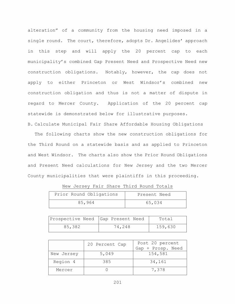
201
alteration” of a community from the housing need imposed in a
single round. The court, therefore, adopts Dr. Angelides’ approach
in this step and will apply the 20 percent cap to each
municipality’s combined Gap Present Need and Prospective Need new
construction obligations. Notably, however, the cap does not
apply to either Princeton or West Windsor’s combined new
construction obligation and thus is not a matter of dispute in
regard to Mercer County. Application of the 20 percent cap
statewide is demonstrated below for illustrative purposes.
B. Calculate Municipal Fair Share Affordable Housing Obligations
The following charts show the new construction obligations for
the Third Round on a statewide basis and as applied to Princeton
and West Windsor. The charts also show the Prior Round Obligations
and Present Need calculations for New Jersey and the two Mercer
County municipalities that were plaintiffs in this proceeding.
New Jersey Fair Share Third Round Totals
Prior Round Obligations Present Need
85,964 65,034
Prospective Need Gap Present Need Total
85,382 74,248 159,630
20 Percent Cap Post 20 percent Gap + Prosp. Need
New Jersey 5,049 154,581
Region 4 385 34,161
Mercer 0 7,378

202
Mercer County Fair Share Third Round Totals
Prior Rd. P.N. Gap P.N. Prosp. N.
Princeton 641 80 388 365
West Windsor 899 132 793 707
The new construction obligation for Princeton is therefore 753,
while the new construction obligation for West Windsor is 1500.
VII. Housing Market Analysis
While not addressing any particular aspect of the fair share
methodology, the court allowed testimony and evidence to be
presented regarding the housing market in New Jersey and the
ability of that market to create affordable housing through 2025.
The municipalities relied on the testimony of Dr. Robert Powell to
support their contention that the obligation recommended by Dr.
Kinsey and FSHC was much too aggressive to be achieved and should
be rejected on that basis. His testimony was intended to show
that the fair share obligation advocated by FSHC and NJBA was
unrealistic when analyzed against the likely pace of residential
development in the next decade. Notably, however, Dr. Powell
addressed only the inclusionary zoning strategy and its
“effectiveness and limitations” in satisfying municipal affordable
housing obligations. Indeed, he testified that the League of
Municipalities had retained him to prepare reports focusing on the

203
limitations of that single mechanism to create affordable housing
in New Jersey through 2025.
Dr. Powell testified that inclusionary zoning depends on a
bargain between municipalities and private developers whereby
towns will grant increased residential densities in return for
developers providing affordable units, typically at a set-aside of
20 percent of the total units. While that bargain is often
attractive to municipalities because affordable units can be
created without municipal financing, it depends on the willingness
of private developers to invest substantial capital in the New
Jersey housing market—-something developers will do only if they
determine it is financially beneficial to do so.
Dr. Powell prepared reports on the likely amount of affordable
housing that could be absorbed by the housing market through
inclusionary developments between the present and 2025. He studied
housing data in terms of residential building permits issued from
1990 through 2010, as well as population and employment data over
the same period. He noted that his projections took into account
the slow recovery from the Great Recession that had characterized
the New Jersey economy, which dampened his estimates for job and
population growth in the State over the next decade. He concluded
that current economic factors would prevent the development of a
robust housing market from now until 2025. His estimates were
based on an assumption that 60 percent of new residential

204
development in New Jersey in the next decade would involve
inclusionary projects. Dr. Powell also noted that recent trends
in the housing market showed increased activity in urban areas and
less interest in suburban communities, although he did admit that
this trend was not particularly pronounced in Region 4 or in Mercer
County. Overall, however, he stated that recent years showed a
significant increase in multi-family new construction and a
decrease in large-lot single family homes as a percentage of total
new development.
Based on his research, and due to uncertainties in the housing
market that made him hesitant to endorse only one estimate, Dr.
Powell created three alternative projections, labelling them Very
Aggressive, Optimistic, and Achievable, as reflected in the
following chart at P-32, slide 9:

205
Throughout his testimony, Dr. Powell focused on the amount of
inclusionary development that he thought was reasonably likely to
occur over the next decade. He was particularly disturbed that
the methodologies proposed by Drs. Angelides and Kinsey were
created in what he perceived to be a vacuum divorced from the
reality of the housing market. While he agreed that there is a
significant need for affordable housing in New Jersey, he saw a
“disconnect” between any fair share methodology and reality when
the methodology did not consider the current characteristics of
the housing market and the likelihood that sufficient new
construction would be built to satisfy the fair share needs
calculated by each methodology expert.
Mr. Jeffrey Otteau also testified for NJBA as an expert
regarding the New Jersey housing market, and opined that the
Alternative Projections for Affordable Housing Production in New Jersey 2015 – 2025
Utilizing the Inclusionary Zoning Strategy
1 2 3 4 5 6 7
Alternative Growth
Assumptions
2015-2025 New Market
Rate Units Average Per
Year
Aggregate 10-Year Total New Units 2015-2025
Adjusted 10-Year Totals
Excluding 20% in Urban Aid
Towns
New Units 2015-2025 Subject to
Inclusionary Development Plan
(Assume 60% of Row 4)
Average Set-Aside
For Affordable Units In all Inclusionary
Developments 2015-2025
(Column 5)
Projected Total New
Affordable Units 2015-
2025
Very Aggressive
40,000
400,000
320,000
192,000
20%
38,400
Optimistic
25,000
250,000
200,000
120,000
20%
24,000
Achievable 18,000 180,000 144,000 86,400 20% 17,280
206
projections of Dr. Powell were too low. Mr. Otteau criticized Dr.
Powell’s forecasts for not adjusting the data to minimize the
effect of the Great Recession, which reflected an extreme
disruption in the housing market and not baseline trends. He
stated that he thought the market could easily achieve the number
of affordable units through inclusionary projects that Dr. Powell
had categorized as “Optimistic” based on the performance of the
market over the last three years. In fact, he stated that the
pent-up need for affordable housing created during the gap period
would increase the demand for affordable housing in the next
decade. Where Dr. Powell had estimated that an aggressive market
through 2025 would produce an average of 40,000 residential
building permits a year, which was his maximum number, Mr. Otteau
countered that an average of 50,000 building permits could be
achieved during the same period. Mr. Otteau noted that more
permits than that had been issued in 1986 and a return to a robust
housing market was possible in the foreseeable future, especially
since the post-Recession recovery had accelerated in New Jersey
and was likely to continue improving at a healthy rate.
Through cross-examination of Dr. Powell and testimony from
Dr. Kinsey, who was also accepted as an expert in the New Jersey
housing market, especially in regard to the development of
affordable housing, it became apparent that Dr. Powell’s testimony
had limited utility. First, Dr. Powell focused exclusively on

207
satisfying the affordable housing need through new construction
provided by inclusionary zoning projects. While that mechanism
had been the primary tool used to satisfy municipal obligations in
the years immediately following the first Mount Laurel decision,
100 percent affordable units have surpassed the inclusionary
mechanism in providing affordable housing since that time. Dr.
Powell simply did not consider those projects in his analysis of
the ability of the housing market to satisfy the need for LMI
housing in the Prospective Need period. He did acknowledge,
however, that they were a very effective way to provide affordable
housing in New Jersey and had a proven track record. He remarked
that such projects typically depended upon developers qualifying
for tax credits, which was beyond the control of the municipality
and thus not as reliable in satisfying municipal obligations as
inclusionary developments. He also noted that changes in tax
policy could affect the likelihood of this mechanism remaining
viable.
Dr. Powell also had not considered how municipalities could
meet fair share obligations by extending affordability controls on
existing units, by qualifying for bonus credits for the creation
of past and future affordable units, by utilizing Affordable
Housing Trust funds supported by developer contributions to help
create affordable units, and by instituting market-to-affordable
programs through which towns use public funds to acquire market

208
rate housing and then subsidize converting those units into
affordable residences. Nor did he consider that mobile home parks
could be considered as another mechanism to satisfy affordable
housing need. Indeed, Dr. Powell admitted that he was not an
expert in municipal compliance strategies to meet affordable
housing obligations, and stressed repeatedly that his opinions
were limited to inclusionary projects only, which was the
assignment he had been given by the League of Municipalities.
Notably, he is not a professional planner, but rather focuses on
the financial and economic side of the real estate market.
In terms of his projections, Dr. Powell acknowledged that
Rutgers was predicting building permits rising to an average of
30,000 per year in the next few years, an amount between his
Optimistic and Aggressive projections. Although he had relied on
studies produced by Rutgers in preparing his own reports, he
disagreed with the Rutgers forecast regarding building permits,
characterizing it as too aggressive. Moreover, Dr. Powell had
refused to consider the poorest of the low income households in
his study of inclusionary developments because he concluded that
they could not afford even the most affordable inclusionary units.
According to Dr. Kinsey, this approach failed to consider that
many very low income households qualify for vouchers that can be
used to subsidize rents in inclusionary projects.
209
Dr. Kinsey provided testimony based on his analysis of data
that he obtained from COAH that 57 percent of affordable housing
units created in New Jersey under the Mount Laurel doctrine had
been developed through 100 percent affordable projects, and 28
percent of the units had been created through inclusionary
developments. He expects both mechanisms to be significant sources
of new affordable housing during the Third Round Prospective Need
period. This evidence showed that Dr. Powell had been mistaken in
concluding that inclusionary developments were the primary
mechanism over time used by municipalities to satisfy their
affordable housing obligations. Based on his familiarity with the
compliance process, which spans more than three decades, Dr. Kinsey
estimated that towns will be able to satisfy approximately 20
percent of their obligations through the use of bonus credits.
Notably, that estimate was based on an analysis of the settlement
agreements FSHC has entered with over 100 municipalities since
Mount Laurel IV was decided in 2015 and over 350 municipalities
filed declaratory judgment actions seeking substantive
certification of their housing plans from the trial courts. Dr.
Kinsey also noted that Dr. Powell had ignored vacant land
adjustments, through which largely developed municipalities can
seek a reduction in their affordable housing obligations due to
the unavailability of vacant land for new residential development.
In addition, Dr. Powell had not examined durational adjustments in
210
affordable housing obligations that towns can seek based upon the
lack of infrastructure necessary for development, such as lack of
utilities, including sewers.
For the Third Round Prospective Need period addressed in these
proceedings, Dr. Kinsey used Dr. Powell’s “Optimistic” estimate
that 24,000 new affordable units could be built through
inclusionary projects, and created a chart he labelled “How the
Prospective Need Can Be Met,” submitted into evidence at Exh. DF
61, slide 6. The chart estimates that Dr. Kinsey’s affordable
housing need number of 163,653 for the Prospective Need period
would lead to construction of 48,865 new units, with the balance
of the obligation being addressed through other compliance
mechanisms, discounts offered through settlements with FSHC, or
attributed to municipalities that have opted not to participate in
declaratory judgment proceedings filed in the wake of Mount Laurel
IV. This chart illustrates how Dr. Kinsey concluded that his
statewide Prospective Need obligation of 163,653 could be met:
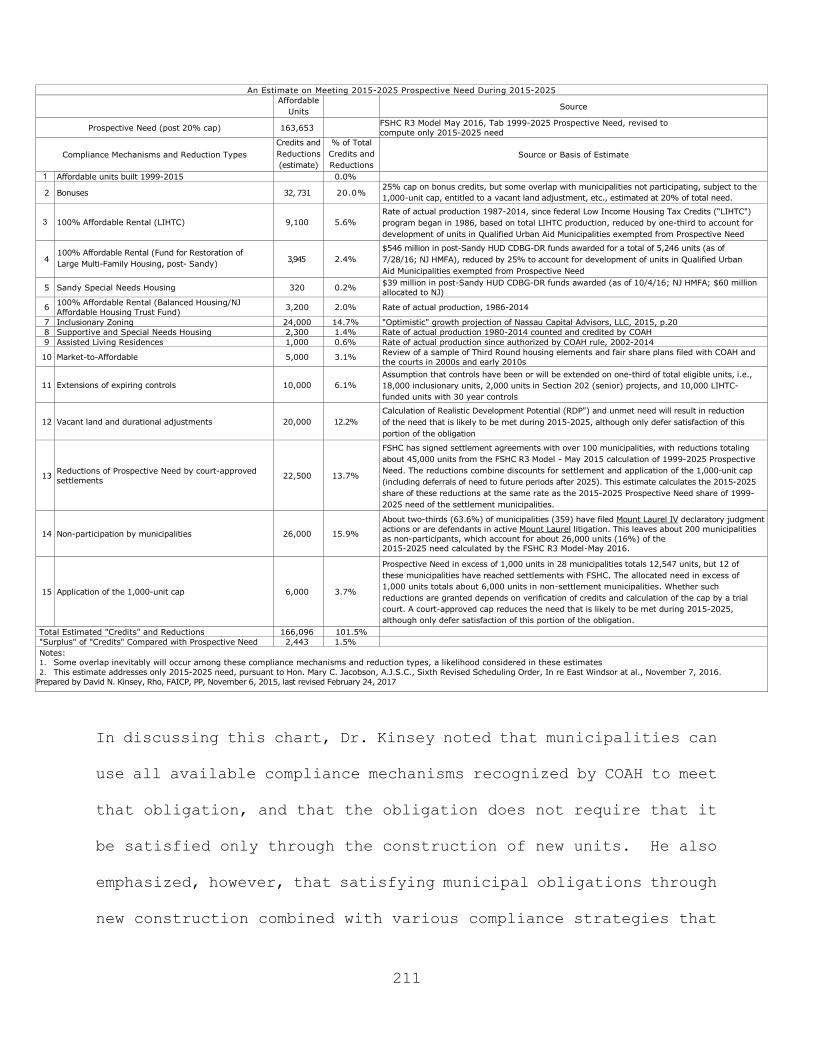
211
In discussing this chart, Dr. Kinsey noted that municipalities can
use all available compliance mechanisms recognized by COAH to meet
that obligation, and that the obligation does not require that it
be satisfied only through the construction of new units. He also
emphasized, however, that satisfying municipal obligations through
new construction combined with various compliance strategies that
An Estimate on Meeting 2015-2025 Prospective Need During 2015-2025 Affordable
Units
Source
Prospective Need (post 20% cap) 163,653 FSHC R3 Model May 2016, Tab 1999-2025 Prospective Need, revised to
compute only 2015-2025 need
Compliance Mechanisms and Reduction Types
Credits and Reductions (estimate)
% of Total Credits and Reductions
Source or Basis of Estimate
1 Affordable units built 1999-2015 0.0%
2 Bonuses 32, 731 20.0% 25% cap on bonus credits, but some overlap with municipalities not participating, subject to the 1,000-unit cap, entitled to a vacant land adjustment, etc., estimated at 20% of total need.
3 100% Affordable Rental (LIHTC) 9,100 5.6% Rate of actual production 1987-2014, since federal Low Income Housing Tax Credits (“LIHTC") program began in 1986, based on total LIHTC production, reduced by one-third to account for development of units in Qualified Urban Aid Municipalities exempted from Prospective Need
4 100% Affordable Rental (Fund for Restoration of Large Multi-Family Housing, post- Sandy) 3,945 2.4%
$546 million in post-Sandy HUD CDBG-DR funds awarded for a total of 5,246 units (as of 7/28/16; NJ HMFA), reduced by 25% to account for development of units in Qualified Urban Aid Municipalities exempted from Prospective Need
5 Sandy Special Needs Housing 320 0.2% $39 million in post-Sandy HUD CDBG-DR funds awarded (as of 10/4/16; NJ HMFA; $60 million allocated to NJ)
6 100% Affordable Rental (Balanced Housing/NJ Affordable Housing Trust Fund)
3,200 2.0% Rate of actual production, 1986-2014
7 Inclusionary Zoning 24,000 14.7% "Optimistic" growth projection of Nassau Capital Advisors, LLC, 2015, p.20 8 Supportive and Special Needs Housing 2,300 1.4% Rate of actual production 1980-2014 counted and credited by COAH 9 Assisted Living Residences 1,000 0.6% Rate of actual production since authorized by COAH rule, 2002-2014
10 Market-to-Affordable 5,000 3.1% Review of a sample of Third Round housing elements and fair share plans filed with COAH and the courts in 2000s and early 2010s
11 Extensions of expiring controls 10,000 6.1% Assumption that controls have been or will be extended on one-third of total eligible units, i.e., 18,000 inclusionary units, 2,000 units in Section 202 (senior) projects, and 10,000 LIHTC-funded units with 30 year controls
12 Vacant land and durational adjustments 20,000 12.2% Calculation of Realistic Development Potential (RDP") and unmet need will result in reduction of the need that is likely to be met during 2015-2025, although only defer satisfaction of this portion of the obligation
13 Reductions of Prospective Need by court-approved settlements 22,500 13.7%
FSHC has signed settlement agreements with over 100 municipalities, with reductions totaling about 45,000 units from the FSHC R3 Model - May 2015 calculation of 1999-2025 Prospective Need. The reductions combine discounts for settlement and application of the 1,000-unit cap (including deferrals of need to future periods after 2025). This estimate calculates the 2015-2025 share of these reductions at the same rate as the 2015-2025 Prospective Need share of 1999-2025 need of the settlement municipalities.
14 Non-participation by municipalities 26,000 15.9%
About two-thirds (63.6%) of municipalities (359) have filed Mount Laurel IV declaratory judgment actions or are defendants in active Mount Laurel litigation. This leaves about 200 municipalities as non-participants, which account for about 26,000 units (16%) of the 2015-2025 need calculated by the FSHC R3 Model-May 2016.
15 Application of the 1,000-unit cap 6,000 3.7%
Prospective Need in excess of 1,000 units in 28 municipalities totals 12,547 units, but 12 of these municipalities have reached settlements with FSHC. The allocated need in excess of 1,000 units totals about 6,000 units in non-settlement municipalities. Whether such reductions are granted depends on verification of credits and calculation of the cap by a trial court. A court-approved cap reduces the need that is likely to be met during 2015-2025, although only defer satisfaction of this portion of the obligation.
Total Estimated "Credits" and Reductions 166,096 101.5% "Surplus" of "Credits" Compared with Prospective Need 2,443 1.5%
Notes: 1. Some overlap inevitably will occur among these compliance mechanisms and reduction types, a likelihood considered in these estimates 2. This estimate addresses only 2015-2025 need, pursuant to Hon. Mary C. Jacobson, A.J.S.C., Sixth Revised Scheduling Order, In re East Windsor at al., November 7, 2016.
Prepared by David N. Kinsey, Rho, FAICP, PP, November 6, 2015, last revised February 24, 2017
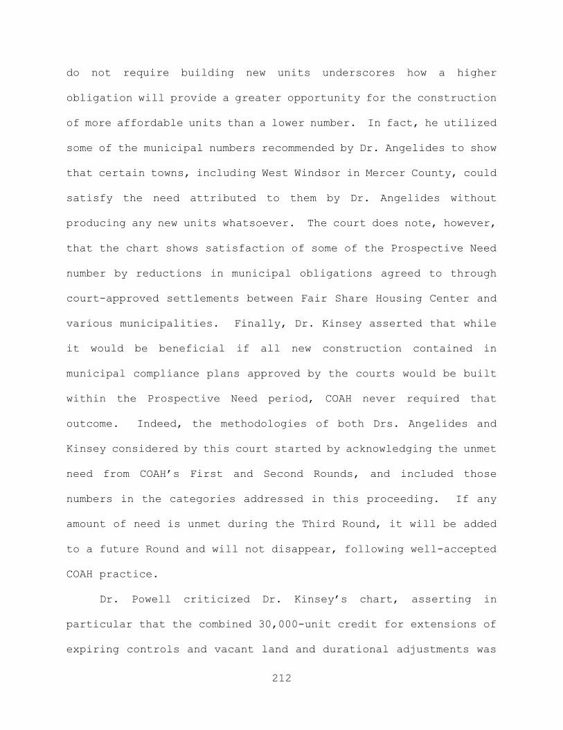
212
do not require building new units underscores how a higher
obligation will provide a greater opportunity for the construction
of more affordable units than a lower number. In fact, he utilized
some of the municipal numbers recommended by Dr. Angelides to show
that certain towns, including West Windsor in Mercer County, could
satisfy the need attributed to them by Dr. Angelides without
producing any new units whatsoever. The court does note, however,
that the chart shows satisfaction of some of the Prospective Need
number by reductions in municipal obligations agreed to through
court-approved settlements between Fair Share Housing Center and
various municipalities. Finally, Dr. Kinsey asserted that while
it would be beneficial if all new construction contained in
municipal compliance plans approved by the courts would be built
within the Prospective Need period, COAH never required that
outcome. Indeed, the methodologies of both Drs. Angelides and
Kinsey considered by this court started by acknowledging the unmet
need from COAH’s First and Second Rounds, and included those
numbers in the categories addressed in this proceeding. If any
amount of need is unmet during the Third Round, it will be added
to a future Round and will not disappear, following well-accepted
COAH practice.
Dr. Powell criticized Dr. Kinsey’s chart, asserting in
particular that the combined 30,000-unit credit for extensions of
expiring controls and vacant land and durational adjustments was
213
based on “soft” data. While that may be true, it is clear that
Dr. Kinsey prepared his estimates with staff from FSHC based upon
their extensive practical experience with the compliance process.
No one else who testified at the trial, except perhaps Mr.
Bernard, a former Executive Director of COAH, had anywhere near
the experience with municipal affordable housing compliance that
Dr. Kinsey had, which was augmented by his working with the staff
of the FSHC over many years. Moreover, Dr. Kinsey even accepted
Dr. Powell’s “optimistic” projection for the number of units to be
created by inclusionary projects rather than his “aggressive”
estimate and incorporated it into the chart. While far from
scientifically precise, the chart is accepted by the court for
what it is—-a series of educated guesses based on significant
practical experience that shows the Prospective Need obligations
recommended by Dr. Kinsey are not unreasonable numbers totally
divorced from reality, as Plaintiffs contend, but rather can likely
be achieved through use of multiple compliance mechanisms,
including new construction. Indeed, that over 100 settlements had
been entered with FSHC as of May 2017 following the Supreme Court’s
returning the substantive certification process to the trial
courts, including several settlements in Mercer County
municipalities that employ many of the strategies included in the
Kinsey chart (i.e., bonus credits, extensions of expiring
controls, inclusionary projects, and 100 percent affordable

214
projects), demonstrates that the obligations calculated by Dr.
Kinsey are not as daunting to many municipalities as Plaintiffs
suggest. In addition, while the chart purported to demonstrate
how a Prospective Need of over 160,000 units could be met, this
court has calculated the Prospective Need to be 85,382. That lower
number makes it even more likely that it is achievable and
accommodates any overestimates that may have been made by Dr.
Kinsey, the uncertainty of projections generally, and the
contention that some of the data used could be considered as
“soft.”
Having provided an analysis of how his Prospective Need number
could be met that included a projection that 48,865 new affordable
housing units were likely to be constructed in the Third Round
through 2025 somewhat constrained Dr. Kinsey when his Gap Present
Need obligation was added to his Prospective Need figure. His
total including Gap Present Need soared to 309,691 affordable
units. Yet, despite this number, which came close to doubling his
Prospective Need number, Dr. Kinsey contended that the maximum new
construction expected would remain at 48,865, somewhat
contradicting his own opinion that the larger the obligation, the
more likely an increased number of new units would be built. He
nonetheless provided an analysis to the court that purported to
demonstrate how his combined Prospective Need and Gap Present Need
obligation of over 300,000 could be met. The chart illustrating
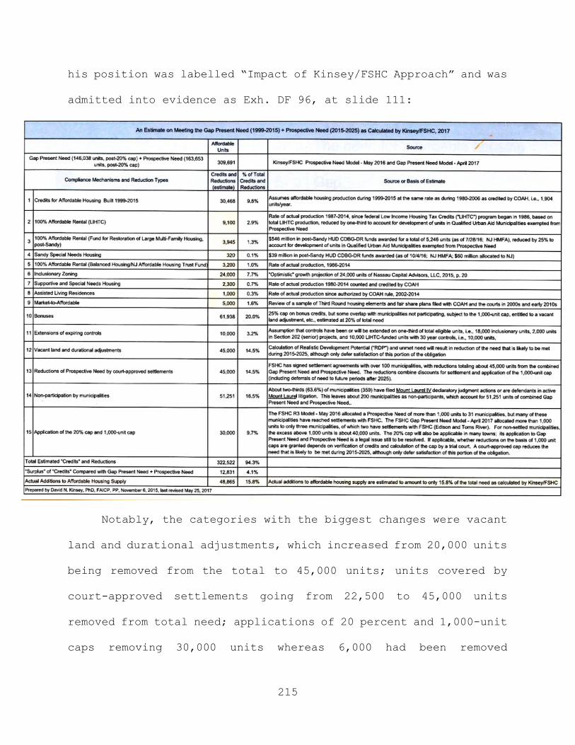
215
his position was labelled “Impact of Kinsey/FSHC Approach” and was
admitted into evidence as Exh. DF 96, at slide 111:
Notably, the categories with the biggest changes were vacant
land and durational adjustments, which increased from 20,000 units
being removed from the total to 45,000 units; units covered by
court-approved settlements going from 22,500 to 45,000 units
removed from total need; applications of 20 percent and 1,000-unit
caps removing 30,000 units whereas 6,000 had been removed
216
previously; and attributing 51,251 units to non-participating
municipalities while 26,000 had been removed from these towns
before. While Dr. Kinsey attempted to justify these significant
increases in order to account for his claim that the total
obligation he recommended to the court was both reasonable and
achievable, his explanations were unsatisfactory and did not
convince the court of the reliability of the much-inflated
assessment. However, since the court’s own analysis of the
methodologies presented in the trial resulted in a combined post-
twenty percent cap Prospective Need and Gap Present Need of
154,581, far below Dr. Kinsey’s number, the court’s rejection of
his final assessment as to how his total recommended need could be
achieved has no impact on the outcome of this case and does not
alter the court’s own conclusions. Indeed, the court found Dr.
Kinsey’s analysis demonstrating that his Prospective Need number
of 163,653 was achievable in the Third Round to be credible. And
that analysis supports the reasonableness and achievability of the
total Third Round municipal new construction obligation found by
the court in this proceeding.
217
VIII. CONCLUSION
As the preceding discussion demonstrates, the parties, expert
witnesses, and Special Master Reading put an enormous effort into
analyzing the most appropriate methodology by which to calculate
municipal affordable housing obligations in the Third Round
affordable housing cycle. The enormity of the effort reflects the
critical importance of the task to the citizens and political
subdivisions in the State of New Jersey. The court hopes that the
formulas adopted and explained in this decision enable Princeton
and West Windsor to promptly finalize new Housing Elements and
Fair Share Plans that satisfy their constitutional obligations to
provide housing affordable to our State’s LMI households. And the
court hopes as well that the work of all involved, and the
transparency of the judicial process leading to the adoption of
the court’s methodology, will assist other courts grappling with
similar issues and —- eventually —- will assist a reconstituted
COAH in ensuring continuing compliance with the Mount Laurel
doctrine.
March 8, 2018


![ADM policy Effective 01st Apr 2017-Updated in OCT19 · d } ] o o ] µ ^W l Z P µ ] o ] v o ] o X .HQ\D $LUZD\V¶ 5HVSRQVLELOLW\](https://cdn.vdocument.in/doc/165x107/5f4eae9b3ee39d094c22b17e/adm-policy-effective-01st-apr-2017-updated-in-oct19-d-o-o-w-l-z-p-.jpg)