Download - January 1970 No. 39
The present report is based on the author's doctoral dissertation,
for which the field research and writing were supported by the
Land Tenure Center, a cooperative program of the Agency for Inter-
national Development and the University of W4isconsin, and by the
Rockefeller Foundation.
January 1970 RP No. 39
SURPLUS L,,,. R AND ECONOMIC
DEVELOPMENT: THE GUATEMALAN CASE
by
Manuel Gollas
The author is presently with the Department of Economics,Universidad Nacional Autonoma, Mexico.
All views, interpretations, recommendations, and conclusions
expressed in this paper are those of the author and not
necessarily those of the supporting or cooperating organizations.
ACKNOWLEDGEMENTS
Licenciado Rafael Piedra Santa, of the University of San
Carlos in Guatemala, and Dr. George W. Hill were very helpful during
the field work of this study.
My adviser at the University of Wisconsin, Professor Kenneth
H. Parsons, gave me assistance and great encouragement.
I also wish to thank Professors Don Kanel and Peter Dorner, of
the Land Tenure Center of the University of Visconsin, for their
guidance in my work. I thank Professor Jeffrey G. Il!illiamson for
his help on the second section of this work, and John Bielefeldt
for his editorial assistance.
Appreciation is given to the Land Tenure Center of the
University of Wisconsin and the Rockefeller Foundation for their
financial support at different stages of this study.
ii

TABLE OF CONTENTS
I.• I NTRODUCT ION ...............................................
11. DESIGN OF THE SURVEY AND SPECIFICATION OF THE PRODUCTION
FUNCT ION ....................................... 20
II. AGRICULTURAL OUTPUT AND SOURCES OF INCCOME..................23
IV. LAND, LABOR AND CAPITAL INPUTS.............................36
V. THE STATISTICAL ESTIMATION OF THE PRODUCTION FUICTION.......50
VI. SURPLUS LABOR, DISGUISED UNEMPLOYMENT, AND THE MARGINAL
PRODUCTIVITY OF LABOR......................................78
VI I. EFFICIENCY, POVERTY AND ECONOMIC DEVELOPMENT...............87
i i i

I. Introduction
This study deals with the economic development of the traditional
sector of the Guatemalan economy. It focuses primarily on the sub-
sistence sector and its problems of modernization.
One major objective of the research is to determine whether a
situation of surplus labor now exists in Guatemalan Highland subsis-
tence agriculture. Another Important objective is to measure the
degree of efficiency in the use of resources by the farmers of that
region.
The study consists of two parts. Part I explains the theoret-
ical framework within which the research was done and briefly
analyzes the history of Guatemala's labor problems. Part I studies
the allocative efficiency of the Guatemalan Indian farmers through
an analysis of the data collected in intense field interviews.
Review of the Literature and Setting of the Problem
Modern 4estern theories of economic development treat problems
of economic growth in very much the same way as did English Clas-
sical economists. Economic dualism, a particularly useful concept
in studying today's problems of development, was first introduced
by the English Classicists to contrast industries with increasing
and decreasing returns.
A modern version of dualism--technological dualism--was
elaborated in 1955 by R. S. Eckaus, 1 who incorporates the factor
proportion problem (the limitations of technical substitutions
among the factors of prodliction)" and emphasizes the imperfections
in the market of the factors of production. 1 Benjamin Higgins has a
version of technological dualism similar to Eckaus', but incorporates
demographic considerations.2 A third version of technological dualism
is that of Harvey Leibenstein.3 Accordinq to Leibenstein, one sector
of the economy stagnates while the other grows. The qrowing sector
is that which exhibits high capital-labor ratio in its production
processes. Technical innovations, according to Leibenstein, are more
likely to be adopted in activities where capital is abundant relative
to labor, and not in activities where labor is the most important
factor of production. The traditional sector, then, becomes stagnant
due to its inability to adopt capital intensive production functions.
The theory of technological dualism is particularly relevant in
the study of underdevelopment because it helps explain the problem
of labor employment. Following is a short outline of the process by
which an economy becomes dual, in accordance with the versions of
dua l i sm descri-bed above.
Labor employment problems in underdeveloped countries stem from
both the use of different production functions in the advanced sector
and in the traditional sector, and from the slow growth of the modern
sector in the face of rapid population growth in the traditional
sector.
1R. S. Eckaus, '=The Factor Proportion Problem in Underdeveloped
Areas," American Economic Review (September, 195.5).
2 Benjamin Higgins, Economic Development (flew York: 1959).
3H. Leibenstein, "'Technical Progress, The Production Function,
and Dual ism," Banca Natlonale del Lavoro Quarterly Review (December,1960).

-3-
The Modern Sector, composed of large scale industry, plantation
agriculture, mines, etc., is characterized by the following features:
I. The production function used in this sector offers very
limited or no range of technical substitution among the factors
of production. Production is carried out with fixed technical
coefficients. That is, the isoquant map is made up of rectan-
gular isoquants. (This assumption of fixed technical coeffi-
cients of production Is a vory d.?at.blc -ssum!tion.)
2. The technology applied to this sector is, in most cases,
capital intensive.
3. The rate of capital accumulation in this sector is slower
than the rate of population growth in the traditional sector.
4. This sector usually does not affect the demand in the
traditional sector for industrial products. That is, the
modern sector fails to create an effective demand for its out-
put in the traditional sector.
The Traditional Sector, engaged in traditional agriculture and
handicrafts, or very small industries, shows these characteristics:
I. The production function for this sector offers a wide ranae
of substitution among the factors of production. That is, pro-
duction is carried out with variable technical coefficients.
The isoquant map is made of isoquants that are convex towards
the origin.
2. The techniques used in this sector are usually labor
i ntens ive.

-4-
3. The rate of capital investment going into this sector is
usually lower than that required to maintain the level of produc-
tivity. The proportion of investments made in this sector by the
modern sector is very small.
4. This sector not only remains stagnant but very often deterio-
rates because:
a. Some of its small industries are unable to compete with
the modern industry of the advanced sector.
b. The growth of commercial agriculture increased the number
of landless peasants or made necessary the cultivation of
marginal poor lands by the displaced peasants.
5. The rate of population growth is very high in this sector.
Given these important characteristics of the modern and tradi-
tional sectors, we can outline how, according to the theory of
technological dualism, unemployment appears in this type-of economy.
As indicated, dual economies frequently have a high rate of
population growth. This additional population must find work in
either the advanced or traditional sector of the economy if unemploy-
ment is to be avoided. However, in dual societies, the modern sector
uses methods of production that are not only capital intensive, but
have fixed technical methods of production; hence, this sector is
unable to absorb the increases in population of the traditional
sector. These increases in population must remain in the tradi-
tional sector. This sector, as shown, uses labor intensive methods
of production with variable technical coefficients; hence, can
absorb the increases in population by making production still more

-5-
4labor intensive and by cultivation of all the available land. As
more and more people are absorbed into the traditional sector, the
marginal productivity of labor decreases until it becomes zero or
even negative; disguised unemployment appears.
This concept of disguised unemployment has been the center of
great debate among theoreticians of economic development and we will
return to it later. At this point it is important to explain how
the excess labor (labor whose marginal productivity is zero or
negative) in the traditional sector can live while they produce
nothing. The answer to this question is found in the internal
organization of the household. Each member of the farm receives a
portion of the total output which is more or less equal to the
average product and not proportionate to his marginal contribution
to the total output. Hence, as long as the average product does
not fall below a minimum subsistence level, all members of the farm
can survive, even if the marginal contribution of some of them is
zero. The average product that each member receives need not be
equal to the subsistence level when the marginal productivity of
labor is zero or negative. Furthermore, when the average output
each member of the household receives is very low, members tend to
4 Given the labor surplus there is no incentive in the tradi-tional sector to produce with high capital-labor production
techniques. As lona as the relative price of labor with respectto capital is low, maximization of output is done along the labor
intensive portion of the isoquant. Technological change does not
help if we accept Leibensteins thesis that technological advances
are usually adopted in the capital intensive production process--
in the advanced sector and not in the traditional one. Hence the
more capital intensive the modern sector becomes dlue to technolog-
ical change, the more difficult it is for it to absorb the excess
labor from agriculture.

-6-
seek employment outside the subsistence sector. They perform odd jobs
in the adjacent towns or they temporarily minrate to plantations of the
commercial agricultural sector.
The belief that conditions of duality--characterized by excess
supplies of labor in the agricultural sector--existend in some Asian
and African countries gave rise to a theory of development described
in W. A. Lewis' pioneer r, "EconomicDevelopment with Unlimited
Supplies of Labor." Probably the central idea of that paper concerns
the possibility of transferring, without reducino agricultural output,
unproductive labor in the agricultural sector to productive uses in
the modern sector at minimal or no cost, thereby creating an economic
surplus to be used in creating new capital.
More recently, Ranis and Fei complemented Lewis' model by
implicitly introducinq in their writlnqs the workings of the agri-
5cultural sector in the process of development of a dual economy.
They also attempted to combine Lewis' model with the notion of the
6critical minimum effort of Leibenstein. The idea associated with
the critical minimum effort is that if the rate of population growth
is larger than the rate Of Orowth of the industrial labor force, the
economy will be trapped in a Ikind of Malthusian equilibrium that is
5J. C. Fei and G. Ranis, "'A Theory of Economic Development,"in C. Eicher and L. "litt (eds.), Aoriculture in Economic Development(t.!ew York: 1l%4), p. 181; and also Ranis and Fei, Deveoment of
the Labor Surplus Economy (N!ew York: 1964).
6H Leibenstein, A Theory of Economic-Democqraphic.Development(Princeton: 1954), andi Economic Backwardness and (Growth MNew York:

-7-
stable for small change in income. In order to get out of the "low
level equilibrium trap" massive infusions of capital are required.
The need for huge doses of capital investments is also associated
with the "bia push" and "unbalance" qrowth theories which are not
discussed here.
The assumption of excess supply of labor in the agricultural
sector of a dual economy--which is probably the most important as-
sumption of the Lewis and the Ranis and Fel models--has been
challenged on both empirical and theoretical grounds. The empirical
work testing this assumption, as evaluated by Kao, Anschel, and
Eicher, does not seem to support It.7 The consistency and theoret-
ical construction of the theory of disouised unemployment as a valid
and useful approach to the problem of economic development of dual
economies also has recently been questioned by D. W. Jorgenson.
The controversy among these authors really amounts to whether
the economies of the underdeveloped countries function according to
the principles put forward by the Classical and Neoclassical school
of thought. 1-e will examine the assumptions of both theories, their
differences and similarities. We will examine the Classical
7C..H. C. Kao, K. R. Anschel, and C. K. Eicher, "DisguisedUnemployment: Survey," in Agriculture In Economic Development,op. cit., p. 129.
8D. Jorgenson, "The Development of a Dual Economy,' Economic
Journal (1961); 'Subsistence Agriculture and Economic Growth,"'paper presented to the conference of Subsistence and PeasantEconomies, Honolulu, March 5, 1965; and "Testina Alternative Theoriesof the Development of a Dual Economy," in Irma Adelman and E.Thorbeck (eds.), The Theory and Desian of Economic Development(Baltimore: 1966 ), p. 45.
-8-
position as explained In the works of Lewis and Ranis and Fel, and
Neoclassical thought as put forward by Jorgenson.
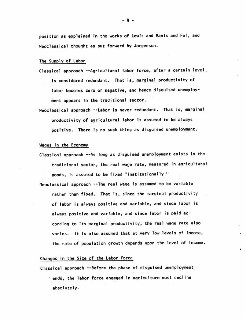
The Supply ofLabor
Classical approach --Agricultural labor force, after a certain level,
is considered redundant. That is, marginal productivity of
labor becomes zero or negative, and hence disguised unemploy-
ment appears In the traditional sector.
Neoclassical approach --Labor is never redundant. That is, marginal
productivity of agricultural labor is assumed to be always
positive. There is no such thing as disguised unemployment.
Wages in the Economy
Classical approach --As long as disguised unemployment exists in the
traditional sector, the real waoe rate, measured in agricultural
goods, is assumed to be fixed "institutionallye:"
Neoclassical approach --The real wage is assumed to be variable
rather than fixed. That is, since the marginal productivity
of labor is always positive and variable, and since labor is
always positive and variable, and since labor is paid ac-
cording to its marginal productivity, the real wage rate also
varies. It is also assumed that at very low levels of income,
the rate of population growth depends upon the level of income.
Changes in the Size of the Labor Force
Cl ass ical approach -Before the phase of d isgui sed unemployment
ends, the labor force engaged in :aqrlculture must decline
absolutely.

-9-
Neoclassical approach --There is no unique behavior of the agricul-
tural labor force during the process of development. The agri-
cultural labor force may rise, fall, or remain constant.
We should point out that in the Classical approach, for the growth
process to take place, it is neither necessary nor sufficient that the
marginal productivity of labor be zero or simply less than the real
wage. What is required is that labor productivity be relatively low
in the traditional sector and that the demand for labor in the modern
sector be smaller than the supply of labor. That is, what is required
is the existence of an excess supply of labor.9
The Classical Approach
The dual economy, according to-the Classical approach, goes through
three more or less well-defined phases. In the first phase, labor can
be supplied to the industrial sector without reducing agricultural out-
put. In the second phase, the transfer is made at the cost of some
reduction in agricultural output. In both phases, if the terms of
trade between agriculture and industry remain constant, and If the
rate of population growth is equal to the rate of agricultural output
growth, then labor is supplied to the industrial sector at a fixed
real wage. The surplus created in the advanced sector is assumed to
be reinvested. As the industrial sector grows, redundant labor in
9Ranis and Fei make a distinction between the case where marainalproductivity is zero (they call this ==redundant labor") and wherethe marginal product of: labor is less than its average product (theycall this 'disguised unemployment").
- 10-
the traditional sector decreases and eventually disappears. This marks
the end of the phase of development with unlimited supplies of labor.
The supply of labor that the industrial sector now faces is upward
slopinq. After this point the marginal productivity of labor in the
traditional sector is positive, but less than the real wage-rate
measured in agricultural goods. This process continues until the
marginal productivity of labor in the agricultural sector is equal to
the real wage-rate. This point marks the beqlnninq of the third phase.
Real waoes in agriculture and industry are the same. "Ithen capital
catches up with the labor supply, the economy enters the /thirdo phase
of development. Classical economics ceases to apply; we are in the
world of Neoclassical economics, where all the factors are scarce,
in the sense that their supply is inelastic.'10
The Meoclassical Approach
The Neoclassical approach to the problem of development of a
dual economy has been expressed in riaorous mathematical models. The
following outline of the Neoclassical approach is the model developed
by Jorgenson.11 The assumptions of this approach in relation to the
supply of labor, the determination of waaes, and the growth of the
labor force are explained above. tWe will now outline the way that
economic growth takes place accordina to this approach. This
1 0 i. A. Lewis, "Unlimited Labor: Further Notes," ' The ,ManchesterSchool (1953), pp. 26-27.
1 1Jorgenson (1961), or,. c~t., and 'Surplus A gricultural Labor and theDevelopment of a Dual Economy,"'Oxford Economic Papers (1967), pp.288-312.

o- 1 -
approach also uses the idea of an agricultural surplus. This surplus
is expressed as an agricultural surplus per head and is defined as the
difference between agricultural output per head and a calculated
critical value of this output per head. 12 If the difference between
these two outputs per head is positive, then part of the labor force
may be transferred from the agricultural sector. The emergence of
the agricultural surplus is essential for the process of development.
Within the Neoclassical framework there is nostationary situation for
an economy as lona as an agricultural surplus and an "economically
viable" advanced sector exist. Provided there is a positive and
growing agricultural surplus, the advanced sector must continue to
grow. The pattern of growth of the advanced sector is determined by
the size of the total population at the time growth begins and by the
size of the oriqinal capital stock. This approach also argues that
sustained economic growth of the economy depends not on the initial
level of capital stock but on the economic viability of the
advanced sector,'which is itself only viable if there is a positive
and growing economic surnlus. As explained above, the existence of
the agricultural surplus and its rate of growth depends upon the
rate of population growth and the arowth of agricultural output.
12The critical value of output per head is defined in thefollowing way. At the beginning of the process of growth, as ateri-cultural output per head increases, all output is consumed. Thisprocess continues until agricultural output per head reaches alevel at which further increases in output per head take the formof consumption of manufactured goods. This critical value is akind of saturation level of consumption of agricultural goods.

- 12 -
Under these circumstances, agricultural technology Increases agricul-
tural output per head; increases in the rate of population growth
decrease It. Hence, the greater the rate of population growth, the
greater the rate of advances in agricultural technology required in
order to have a positive and growing agricultural surplus. If
advances in agricultural technology are not possible, sohne kind of
population control is required in order for the agricultural surplus
to exist and grow.
As we have said, the Classical approach reduces to the Neoclas-
sical one after redundant labor disappears--after the phase of dis-
guised unemployment ends. It seems, then, that the two approaches
have different implications only for situations where disguised un-
employment exists. Hence, the evaluation of the Classical versus
the Neoclassical theory of development of dual economies has meaning
only when they are compared in economies where disguised unemploy-
ment is said to exist. Here lies the relevancy of conducting
empirical research on the existence of disguised unemployment.
Empirical Tests
Empirical research to measure the existence of disguised un-
employment has been conducted in many countries using different
approaches.13 The evidence presented to support the existence of
a high percentage of disguised unemployment in underdeveloped
countries is numerous, but often not very convincinQ. The same
13 See Rao, Anschel and Elcher, o1. cit., pD. l3 "- 1h1.

- 13 -
can be said of research conducted to reject the existence of disguised
unemployment.
Research followed what have been called the "direct" and "indirect"
methods of measuring disguised unemployment. 14 The direct method con-
sists of: (a) studies in which labor requirements to produce the
present level of agricultural output and the present level of agricul-
tural labor force are calculated. The difference between what is
available and what is required is regarded as disguised unemployment;
(b) studies that examine historical cases in which by some event or
calamity a portion of the agricultural labor force has been removed
from the agricultural sector; whether agricultural production decreases
or does not decrease after this event or calamity is taken as evidence
that disguised unemployment was not or was present in the agricultural
sector; and (c) anthropological works which consist of budget analysis,
the study of the household behavior, and the way in which individuals
make economic decisions.
The indirect method used in measuring disguised unemployment and
150the implications of the Classical approach consists in the analysis
of time series in order to test: (a) whether historically the supply
of labor faced by the industrial sector has ever had the characteristics
claimed hy the Classical or Neoclassical theory; that is, whether the
1 Ibid., p. 135.
15 For the source of these implications (c, d, and e), derivedfrom the Classical approach, see Jorgenson (1965, 1966), 00. cit.
- 14 -
supply of labor has been perfectly elastic and if the real wage has
been fixed institutionally during the time when disguised unemployment
is said to have existed; (b) if the absolute size of the agricultural
labor force has declined (Classical approach) or did not follow a
definite pattern (Neoclassical approach) during the process of dis-
guised unemployment; (c) whether labor productivity in the advanced
sector remained constant during the period of disguised unemployment
(Classical approach) or was always rising (Meoclassical approach);
(d) if in the advanced sector the rate of growth of output and employ-
ment increased over time (Classical) or the rate of growth of both
variables declined over time (Neoclassical); (e) whether in the
advanced sector of the economy the capital-outout ratio declines
through the phase of disguised unemoloyment and the rate of growth
of capital increases over time (Classical) or the capital-output
ratio and the rate of growth of capital become constant as the
process of development advances (Neoclassical).
I.!e think it very important to know if the economic variables
of a given economy behave accordinq to the Classical or Neoclassical
postulates. The policy implication of knowinq or not knowing the
magnitude and behavior of these variables can hardly be over-
emphasized.
We have outlined the main features and assumptions of the two
modern approaches to the development of a dual economy in order to
establish a framework of reference for the study of the Guatemalan
economy. Guatemala has the characteristics of a dual economy: a
modern sector (industries in Guatemala City, Ouetzaltenanio, etc.,

- 15 -
and a market-oriented agriculture in the Lowlands); and a traditional
sector (subsistence agriculture in the Highlands and small handicraft
Indian industries). The Highlands are briefly described below.
Description of the Guatemalan Highlands
Population
According to the 1964 Census, Guatemala continues an overwhelm-
ingly rural country. In 1964, 71 percent of the total population was
resident in rural areas, only a slight reduction from the figure of
75 percent in 1950. The total population of the Republic is reported
to have increased by 53.5 percent in the 14-year intercensal period,
at an annual rate of increase of 3.1 percent per year. The 1964
Census data suggested increases of 33 percent in the rural population
and 105 percent in the urban population for the entire country between
1950 and 1964. However, the definition of urban population in the
recent census differed from that used in 1950, thus invalidating
direct comparison of the Census data. Adjustment of the 1964 data,
using the 1950 definition of urban residence, suggests increases of
45.7 percent in the rural population and 77.1 percent in the urban
population (see Table 1).
The Highlands, as here defined, include all the lands that lie
at altitudes ranging from one thousand to three thousand meters in
the seven departments of Chimaltenanno, Quiche, Totonicapan, Huehue-
tenango, Quezaltenango, San Marcos, and Solola. These seven depart-
ments are the most thickly populated region of Guatemala, with a
population density of 178.1 inhabitants per square mile, compared

- 16 -
Table 1. Rural and Urban Population Change, Guatemala, 1950 to 1964
1950
Rural
933,025
1,161,385
2,094,410
Urban Total
162,546 1,095,571
533,912
696,458
1 ,695,2972,790,868
1964
I1I,212,886 . 335,323 1,548,209
1_1633,526
2,846,412
1,102.,738
I ,438,061
2,736,264
4,284,473
a1964 (adjusted)a
1,301,284 246,925 1,548,209
19,749,422
3,050,706
988,842
1,235,767
2z,738,2644,286,473
Percent Increase (adjusted)
39.5 51.9 41.3
50.6
45.7
84.8
77.1
61.4
53.5
aThe 1964 census data were made comparable with the 1950
data by considering as urban only those population clusters which
had 2,000 inhabitants or more, or had been considered as urban in
1950, even though they had fewer inhabitants. (Data supplied by
L. Schmid of the Land Tenure Center, University of Wfisconsin.)
Region
H i gh lands
Other
Tota I
Highlands
Other
Total
Highlands
Other
Total
Highlands
Other
Total
- 17 -
to 109.2 for the entire country, or to 155.3 for all Guatemala if the
Spanish settled department of Peten is excluded. The Highland region
accounts for 36 percent of the population of Guatemala.
The population of the Highlands region increased by 41.3 percent
in the period 1950-64, an annual rate of increase of 2.5 percent.
The Highlands urban population increased by 51.9 percent whereas the
rural population increased by 39.5 percent. All the departments in
the region participated in the large urban increase except for
Totonicapan, where the urban increase was only 3.3 percent.
Land Concentration
Guatemalan agriculture is characterized by a concentration of
land in a few large farms. According to the 1950 Agricultural Census,
there were 348,687 farms in Guatemala which occupied an area of
3,720,833 hectares. The average size of farms was 10.68 hectares.
The Census data Indicated that farms which were 45 hectares or larger
(0.31 percent of total number of farms) contained 50.35 percent of
the land; farms of less than 7 hectares in area (88.35 percent of the
total number of farms) contained only 14.33 percent of the farmland.
At the time of the 1950 Census the Highlands of Guatemala con-
tained 162,289 farms (46.54 percent of the nation's farms), and they
occupied 992,000 hectares (26.62 percent of the total farmland),
so the average farm area in the region was 6.11 hectares. The High-
lands contained a larger proportion of the nation's small farms than
did other regions, but proportionally fewer large farms--54.17 per-
cent of the farms less than 0.70 hectares, but only one farm larqer
than 9,020 hectares.

- 18 -
According to the-1964 Census, the Highlands contained 27 percent
of Guatemalan farmland and 47 percent of the farms. The average farm
size in the Highlands was 6.1 hectares, compared with the national
average of 10.7 hectares. The Census also indicated that in the
Highlands, 31 percent of the farmland was controlled by 0.2 percent
of the farmers; a slightly less concentrated pattern of land distribu-
tion than for the nation as a whole where 50 percent of the farmland
was controlled by 0.3 percent of the farmers. The concentrated
nature of land distribution in the Highlands can be illustrated
another way--50 percent of the farms were less than 1.4 hectares In
1964.
Climate and Cultural Characteristics
In general, the Highlands have a temperate climate, which in
the highest zones becomes relatively cold in December, January, and
February. Like the remainder of the country, it has two distinct
seasons of about equal length. The wet season (winter) lasts from
May until November; the dry season (summer) occurs during the
remainder of the year.
There is little level land in the mountainous terrain, so most
of the crops are planted on slopes, some at extremely precipitous
angles. The fields are usually divided Into strips, separated by
narrow margins marking Individual holdings. Much of this land has
been under cultivation for many centuries.
From a cultural viewpoint, the homogeneity of the region is
readily observable. All the inhabitants are descendants of the

- 19 -
Mayan Indians. Most people still converse in one of the many Mayan
dialects, and the women, particularly, dress in traditional costumes.
With few exceptions, these people follow the planting and cultivating
practices handed down through many generations.
In an economic and social sense, the region is equally homoge-
neous. Poverty is the general rule. The few centavos that the Indian
makes when he is able to find work away from home are needed to buy
more corn. Corn is the mainstay of his diet but his farm is not suf-
ficiently large to provide enough for sustenance. The rate of
illiteracy is overwhelming: two-thirds of the heads of families in
this study could neither read nor write. The population of the area
has little or no voice in the government of the country.
The purpose of the study can be stated very simply: it intends
(a) to see if the traditional sector of the Guatemalan economy has
had and continues to have the characteristics of, and functions
according to, the postulates put forward by the Classical and Neo-
classical theories of growth; and (b) to analyze the policy implica-
tions of the results.
Through analysis of the data collected from a sample of tradi-
tional Highlands farmers, the hypothesis of disguised unemployment
in the traditional sector of today's Guatemalan economy is tested.
Efficiency in the use of resources by the traditional Highlands
farmer is also measured.

- 20 -
II. Design of the Survey and Specification
of the Production Function
Analysis of the Guatemalan Agricultural Census of 1950 indicated
that 21.3 percent of the nation's farms were less than 0.7 hectares
(micro-fincas), 67.1 percent were between 0.7 and 7.0 hectares (sub-
familiares), 9.5 percent were between 7.0 and 45 hectares (fincas
familiares), and the remaining 2.1 percent were over 45 hectares
(fincas multi-familiares). There was a higher concentration of small
farms in the western Highlands, the area of this study: 24.8 percent
were micro-fincas, 64.8 percent were fincas sub-familiares, 9.1 per-
cent were fincas familiares, and only 1.3 percent were fincas multi-
fami1 i ares.
Since this study is concerned with traditional agriculture, the
sample was chosen from farms of family size or smaller.
A series of municipios (counties) were selected in the Highlands
which were believed to yield a representative sample of traditional
agriculture as practiced in the region. Three municipios were chosen
from the Department of Chimaltenango, and two from the Department of
Solola, but all of these within the Cakchlquel linguistic area.
Three were chosen in the first department because it has a more
heterogeneous system of agriculture than the others in the study,
with greater variation in soil, altitude, and other factors. Two
municipios were selected in the Department of Quiche, two in Toto-
nicapan, one in Quezaltenango, and one in Solola--all representing
the Quiche linguistic area. In order to include the linguistic area
of the Main, two municipios in the Department of Huehuetenango

- 21 -
and two in San Marcos were also selected, The Cakchiquel, the Quiche,
and the Mam are the three major linguistic groups of the Maya who
inhabit the Western Highlands. To complete the sample, three addi-
tional municipios were also selected from Huehuetenango to represent
minor linguistic groups: two for the Kanjobal and one for the
Agucateca.
Since the Agricultural Census of 1964 had been completed only a
few months before this work began, its lists of farmers and farm sizes
were used. From these lists a random sample in each aldea was drawn.
This method yielded approximately 400 farms, from which about 348
interviews were obtained.
The Production Function and Its Properties
The method used in studying the allocative efficiency of resources
among Guatemalan Hiqhland farmers was to fit Cobb-Douglas single equa-
tions to cross-sectional data collected by intensive questionnaire
interviews of 348 randomly chosen farmers.
The functional form of the Cobb-Douglas production function is:
Y = AX Xb2 x bI " "bn (I)1 2 In
where Y is output, Xi the inputs, A is a constant and b. refers to
the transformation ratio when X. is at different magnitudes.
The Cobb-Douglas function becomes linear in the logarithms, hence:
log Y = a + b I log X1 +* b i log Xi + bn log X ((2)

- 22 -
The marginal productivity of the factors of production indicate
the returns that might be expected, on the average, from the addition
of the various resources. The marginal physical product of a given
input, then, is the partial derivative of the output with respect to
that input, all other Inputs held constant. Hence differentiating
equation (1) with respect to X I we write:
Ib I . . .xbI . . n I 0---0M(3)X I-
In order to obtain the elasticity of production of a factor, we
use the concept of marginal product. The elasticities of production
indicate the percentage change in output with respect to a percentage
change in Input. Hence, from (1) and (3) we can write:
Y X YVXi
Therefore, in the Cobb-Douglas function, the elasticities of produc-
tion are given directly by the respective input exponents and they
are constant over the entire Input-output curve,
Production functions of the Cobb-Douglas type permit observation
of the phenomenon of returns to scale. The sum of the estimated input
coefficients is taken as an Indication of the returns to scale. If
this sum is smaller than one, it indicates decreasing returns to
scale; if it is larger than one, there are increasing returns to
scale; while if the sum of exponents is equal to one, there are
constant returns to scale.

- 23 -
Under conditions of perfect markets, the optimum allocation of
resources is achieved when the marginal productivity of each factor
is equal to Its real wage. Hence we can write:
bY b. y WISX I X I P
where Wi is the money wage of factor I and P is the price of the
product.
Under the situat.lQn of perfect markets, then, we can directly
compare the marginal productivity of a factor to its opportunity
cost in order to detect the degree of efficliency ,in the allocation
of resources. If the ratio of marginal.productivity of a factor to
its opportunity cost is less than one, too much of the given resource
is being used. If the ratio of marginal productivity to opportunity
cost is more than one, too little of the given factor Is being used.
Maximum efficiency occurs when marginal productivity of a factor is
equal to its opportunity cost.
The next sections specify the variables, and estimate the
production elasticities, marginal productivities, and efficiency
ratios for the sample of farmers in the study.
I!l. Agricultural Output~and Sources of Income
Malze--the Basis of the EnterpriseMaize is the principal food of every Indian so Its culture pre-
dominates in the Highlands. Preparation of :the land for planting,
actual planting, and the first, second, third, and sometimes the

- 24 -
fourth cultivation to control weeds and to repair storm damage, and then
finally harvesting, shelling, and storage extend the process to a year
round operation. Only a few weeks after the seed ears have been stored,
it is time to start clearing the dried stalks and accumulated vegetation
in the fields so that they can be burned.
Beans are another important item in the indigenous diet. Planting
techniques vary between localities, partly because of cultural deter-
minants which many anthropologists have described, and partly because
of the dictates of experience. While "large" farmers will plant whole
fields of corn and beans separately, hoe culture permits combining both
in the same field, with corn, pole beans, and Jima beans in the same
planting hole.
Potatoes are planted between the rows and when that is done,
lesser amounts of other crops are planted, so that here and there will
be a squash, a pumpkin, and frequently a lima bean stalk. If the farmer
has a special field of potatoes, even though it measures only two or
threee cuerdas in size, he has reached a level above the average
peasant's described here, because he has land and enough money to
take a risk on a cash crop in addition to the milpa which he plants
elsewhere to insure his family's subsistence. Storage facilities
being deficient and crude, and harvests from the plots not large,
every advantage that nature might provide has to be seized if
tortillas are to be on the table regularly; otherwise the peasants
willI suffer a long dearth of food before harvest.
Completion of the third and final round of cultivating winter
fields varies within the region from late July to September.

- 25 -
Occasionally, the hill farmer has to cultivate still again very late
inthe season. After the cultivation cycle has been completed, the
farmer is free to look for work away from home--he may spend one or
two months picking coffee In the cafetales that abound below the
altiplano and on the Pacific slopes. With the advent of cotton as a
major export crop following World War I!, some of the Highlanders
began to work in its harvest during the months of November,
December, and January.
Principal Crops and Yields
From the preceding description, any breakdown of the farm enter-
prise into precise units by crops is obviously difficult. All of the
farms had some corn plantings (see Table 2), with an average of 1.03
hectares of "sole" corn plantings per farm. Corn yields ranged from
14.4 quintals per hectare in Huehuetenango to 24.4 quintals in
Quezaltenango, with a regional average of 18.96 quintals per hectare
(see Table 3). The high yield in Quezaltenango may have been
obtained because most of the farmers used chemical fertilizer; such
use did not occur much in the other departments. In Huehuetenango
not a single operator had used any.
Wheat was cultivated on 130 farms. The total area planted was
128.1 hectares, about 36 percent of the area planted to maize. Two
of the departments, Quicheand Huehuetenango, planted little or no
wheat. The highest concentration of wheat farmers was found in
Solola and San tMarcos. Solola had the highest yield, 27.9 quintals
per hectare, and since a large portion of the farmers in that
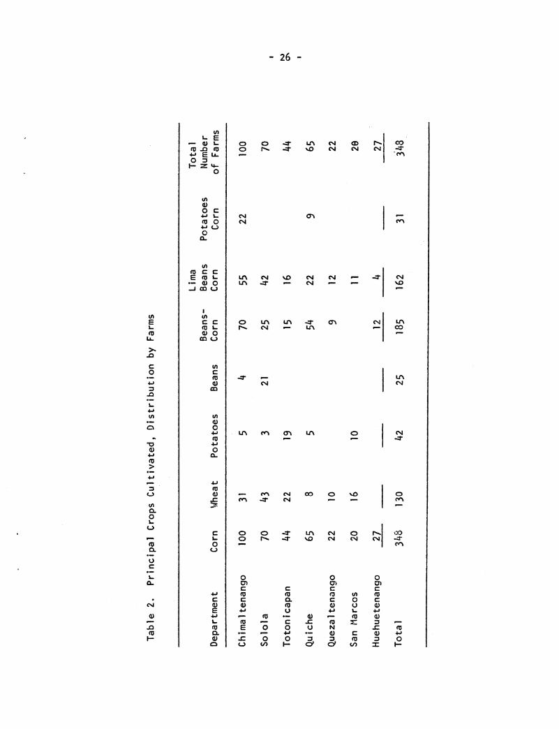
- 26 -
o) 0U'% n C%4I CD N. Co rF* - . " ,o (N ( C-T
C*, (NON
0 £4-' ELL-
0
0OC
004-) 1.0
0
.3U)
C c r
0CC
m OL
(DC
00
C
0
0
U4
0
04-'0
a-
4.)0
-c
I..0
C-)
4.
4.)L:
00 0
(0)cCL c013 4) u)
4- u 41I L 4.
E 0 00u
2 0 0 U N(A ' -- 0 C 0
UN C 0 %.D
0 In In O O
,-. e C% 00 0
m _z. C4
0 0 -" In e J0 r-% -- o
_-- C%4
0 N
c0 o
row=fal
HGM
EL
LL.
C
0*am
4.J
4-J
U)
C.
0
4,
(-)
An
C.0
m..C.)
.CL
a-
04-0
Table 3. Area Cultivated (Hectares) and Yield (Quintals) of Principal Crops
Corn Wheat Potatoes Beans
Yield per Yield per Yield per Yield perDepartment Area Hectare Area Hectare Area Hectare Area Hectare
Chi ma Itenango
Solola
To toni capan
Quiche
Queza 1 tenango
San Marcos
Huehuetenango
Total
119.4 20.4
104.2 16.4
14.8 17.6
58.3 21.3
15.0 24.4
18.5 20.7
29.2 14.4
359.4 19.0
18.3
53.3
7.6
5.8
30.1
13.0
18.3
27.9
17.3
13.0
22.4
18.3
128.1 23.0
1.2
0.5
2.7
0.6
235.9
134.7
60.0
145.2
0.9 210.0
5.9 134.0
0.8
8.2
8.6
11.0
9.0 10.8
- 28 -
department grew wheat, the overall regional yield is unduly influenced--
it amounted to 23.0 quintals per hectare. Without Solola, the regional
average would drop to about 19 quintals per hectare, closer to that
found in the other departments.
Potatoes represent an insignificant part of the farm enterprise,
and the crop was included separately only to indicate its scarcity in
the subsistence economy. A total of 42 farms reported they had
separate potato plantings, but the total area planted amounted to
only 5.9 hectares. Even if the area of land in which potatoes were
interplanted with corn is added to this, the total is only 10.6
hectares, or less than three percent of the amount of land in corn.
If the department of Totonicapan is removed from the total, the
average yield would be about 197 quintals per hectare, demonstrating
the production possibilities for this crop in the Highlands.
Frijoles de suelo were grown as a separate crop on only 25 of
the 348 farms studied, whereas frijoles de milpa, or frijoles de
vara, were intertilled on 54 percent of the milpas and occupied
about 45 percent as much land as did corn. However, the yieIds of
the two varieties of beans were radically different; the first
yielded 10.8 quintals per hectare, while the other yielded only
1.7 quintals.
The haba (similar to the lima bean) was another crop often
interplanted with corn, appearing on 162 farms. Yields with such
beans were slightly higher than for the other varieties, averaging
2.0 quintals per hectare, with no marked variation between
depa rtments.
- 29 -
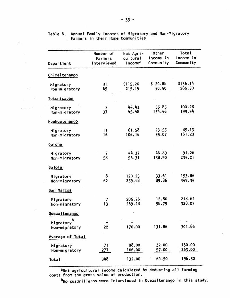
Value of Agricultural Output and Complementary Income: Migratoryand Non-Miratory Farmers
There are three principal sources of Income for the people of
the Highlands: farming on their own where a substantial part of the
production is consumed directly; supplementary employment within
their home communities; and earnings received as a migratory farm
laborer in commercial agriculture, mostly in the coastal region.
The gross value of annual production per farm varies, as would
be expected, directly with the size of farm. The average value of
16production per farm in this study was Q207.55 (see Table 4). Of
this amount about one-half was sold and the other half consumed by
the family. If the area cultivated per farm is considered, the
farms with smaller cultivated areas sell a smaller proportion of
the total product than do the larger farms (see Table 5). Although
the proportion of the crop sold is not correlated precisely with
the area cultivated, farms under 1.5 hectares in size, about two-
thirds of the total number, sell less than 40 perco;it; ;hile farms
over 1.5 hectares in size sell about 56 percent of the c'op. The
net value of farm production, after deduction of cash costs, was
Q155. Thus the average gross value of farm output per person was
Q42, whie the corresponding figure per man unit was approximately
Q84.
Since the Highland area is a low income farming area from
which a considerable number of campesinos migrate annuai ly to the
16 0ne Quetzal = One U.S. dollar.

Table 4. Average Value (Quetzals) per Finca of Gross Annual Production ClassifiedAccording to Area Cultivated (Hectares)
Under 2.5 Ha.0.5 and
Department (Ha.) 0.5-0.9 .O-i.4 l.5-1.9 2.0-2.4 over Average
Chimal tenango
To toni capan
Queza I tenango
Qui che
Solola
Huehuetenango
San Marcos
Average
37.70
37.95
66.55
67.05
62.90
33.55
50.95
118.35
73.15
72.60
106.40
60.75
49.30
69.00
93.70
197.95
99.35
75.00
169.75
194.90
207.00
148.20
179.40
248.30
92.00
719.00
231.65
183.75
97.00
271.50
239.45
242.00
339.50
468.50
238.60
211.35
446.80
299.20
498.50
I ,190.00
496.25
621.05
420.65
757.50
629.55
208.00
69.90
382.70
145.95
308.35
108.05
297.20
207.55
0
Table 5. Value of Annual Gross Production Sold per Finca (Quetzals)
Average Value PercentageNumber Gross Annual Average Value Product Sold
Hectares of Production Product Sold per FincaCultivated Fincas per Finca uper Finca (By Value)
Under 0.5 83 50.95 17.30 34.0
0.5 - 0.9 92 93.70 33.40 35.7
1.0 - 1.4 53 179.40 70.00 39.0
1.5- 1.9 46 239.45 120.35 50.3
2.0 - 2.4 27 299.20 125.30 41.9
2.5 and over 47 629.20 393.30 62.5
Total 348 207.55 102.35 4993

- 32 -
coastal region for employment as agricultural laborers, the net family
incomes of the campesinos interviewed were calculated separately ac-
cording to whether or not they were migrant farm laborers. Twenty
percent of the respondents were migrant workers (see Table 6).
The net farm income of the migrant was smaller in all departments
than the net farm income of the cultivator who did not migrate, al-
though the difference was negligible in Totonicapan. For the depart-
ments as a whole, net farm income of all migrants was Q99.63, compared
with Q169.90 for those not migrating--70 percent higher for non-
migrants.
Farm incomes were also supplemented by incomes earned in the
local communities by working as hired laborers, craftsmen, or petty
traders. Incomes so earned were again not evenly distributed.
Migrant farm workers were less successful in earning extra incomes
locally than were those who did not migrate. In the departments as
a whole, the average annual supplementary earnings received locally
were Q27.93 for the migratory laborers and Q98.8 1 for those who did
not migrate (see Table 6).
As noted in Table 7, the average combined incomes earned locally
by the respondents was Q239.22 per family. Again the incomes of
non-migrants were much larger, more than twice as large on the
average as the migrants', Q268.71 compared to Q127.56 .
The source of: these supplementary earnings varied greatly among
commun it ies. I n the commun ities where raw cotton was ava ilabl!e, and
in some cases wool, spinning and weaving provided a supplement to
farm earnings, especially in the villages studied in San Marcos,
- 33 -
Table 6. Annual Family IncomesFarmers In their Home
of Migratory and Non-migratoryCommunities
Number of Net Agri- Other Total
Farmers cultural Income in Income inDepartment Interviewed Incomea Community Community
Ch ima Itenango
MigratoryNon-migratory
Totonicaan
Migratoryfon-mi gratory
Huehuetenango
MigratoryNon-mi gratory
Quiche
MigratoryNon-mi gratory
Solola
MigratoryNon--migratory
San Marcos
MigratoryNon-migratory
Queza 1 tenangob
MigratoryNon-migratory
Average of Total
MigratoryNon-migratory
Total
3169
737
1116
758
862
713
22
71277
348
$115.26215.15
44.4345.48
61.58106.16
44.3796.31
120.25259.48
205.76269.28
170.00
98.00166.00
132.00
$ 20.8850.50
55.85154.46
23.5555.07
46.89138.90
33.6189.86
12.8658.75
131.86
32.0097.00
64.50
$136.14265.50
100.28199.94
85.13161.23
91.26235.21
153.86349.34
218.62328.03
301.86
130.00263.00
196.50
aNet agricultural Incomecosts from the gross value of
calculated byproduction.
deducting all farming
bNo cuadrilleros were interviewed in Quezaltenango in this study.

- 34 "
Quiche, and Totonicapan. Not only were the returns profitable, but
these supplementary tasks also provided the basis for a permanent
cottage industry. This situation allowed the families who participated
a permanent residence; they did not become exposed to the problems
that plague migrant labor families.
As noted above, only one-fifth of the 348 family heads had
participated the preceding agricultural year in the annual migration
of harvest workers to the coffee and cotton haciendas of the Pacific
Coastal slopes. The migrant workers did not come from all departments
in equal proportions. Moreover, workers seemed to come from certain
caserios within departments, while not from other communities in the
same department. For example, among those interviewed in the depart-
ment of Chimaltenango, none who lived in Chimazat participated in the
migrant movement; those who went were from the farms in the Comalapa
and Sta. Apolonia municipios. The same was true of Solola--the
campesinos of Las Canoas, an aldea of San Andres Semetabaj, stayed
home, while almost all among those interviewed from the department
who went were from Santa Catarina Ixtahuacan.
As would be expected, the lower income farms contributed most
of the migrants. The data suggest that 25.0 percent of operators
of farms with less than one hectare of cropland participated in the
migrant stream to the coast, along with 22.0 percent of the operators
of farms with more than one but less than two hectares of cropland,
and only 14.0 percent of operators from farms with more than two
hectares of cropland.

- 35 -
Contrary to expectations, there was but slight difference in the
average age of the "migrant" and the operators as a whole--40.2 years
and 42.7 years, respectively. Generally migratory laborers come from
the younger age groups, but here the low average farm income operated
as a "push" factor, causing the migrants to come from all age groups.
The average migrant returned home with Q31.55 cash in his posse-
ssion, an average of approximately Q15.00 per month for the two months
sojourn on the coast; compared to prevailing farm wages in the High-
lands, this figure is only a little over the highest daily rate paid
in the area, which was 50 centavos.
When incomes from all sources are combined, the average income
reported per family for non-migrants was Q263.00 and for migrants
Q161.55, with an overall average.of Q228.05 (see Table 7). Clearly
the migrants are poorer by far. Although the net cash earnings
reported from such .employment were only Q31.55, the workers did have
some sort of subsistence while they were so employed.
Table 7. Comparison of Total Incomes for Migrants and Non-Migrants
Non-Migrants Migrants Total
Average net incomefrom agriculturalproduction 166.O0 98.00 132.00
Income from empl1oy-men t i n commun ity 97b.00 32.'00 64.50
Net i ncome frtomemployment asmigrant farm worker _ ___31.55 31.55
TotalI 263.0O0 16!. 55 228.05
- 36 -
IV. Land, Labor and Capital Inputs
Land Input
Land Use and Size of Farm
Land has only two major use classifications in the Highlands--
cropland and woodlot. The average area of land among the sample farms
allocated to pasture, woodlot and cultivation was 0.21, 1.03, and 1.49
hectares, respectively. Woodlots were found on 58.6 percent of the
farms. Pasture lands (accounting for 8 percent of all land in farms)
were found only at the highest altitudes--over 2,500 meters in
altitude--and then only in the extreme western part of the region.
Only 14.6 percent of the farms contained pasture, and only in Toto-
nicapan and San Marcos was there a significant incidence of pasture
land.
The sample population was classified according to farm area and
also by area cultivated. The average farm area for the sample was
3.00 hectares, while cultivated area was 1.49 hectares (see Table 8).
The average farm area and cultivated area was computed for each of
the six farm size classes used in the classification of the sample
data (see Table 8). This analysis indicates that as the farm area
increases, the proportion of the farm cultivated diminishes. Farms
less than 0.50 hectares in size cultivated 79.3 percent of the land,
while those in excess of 2.49 hectares cultivated 41.6 percent of
the l and.
The largest farm in the sample was 42.24 hectares; two farms
had an area in excess of 20 hectares and only 13 (5.2 percent) had

Table 8. Sample Farms Classified by Total Farm Area and by Cultivated Area
Classification by Total Area Classification by Cultivated Ar=aAverage Average of AverageTotal Cult. Farm Cult.
Area Class No. of Percent- Farm Farm Area No. of Percent- Farm
(Hectares) Farms age Area Area Cult. Farms age Area
0.00 - 0,49 54 15.5 0.29 0.23 79.3 83 23.6 0.28
O.50 - 0.99 65 18.7 0.73 O.56 76.7 92 26.7 0.72
1.00 - 1.49 42 12.1 1.24 0.92 74.2 53 15.2 1.25
1.50 - 1.99 47 13.5 1.75 1.18 67.4 46 13.2 1.73
2.00 - 249 30 8.6 2.20 1.66 75.5 27 7.8 2.18
Over 2.49 110 31.6 7.11 2.96 41.6 47 13.5 4.80
Total 348 100.00 3.00 1.49 49.7 348 1O0.O0 1.49
a
I
- 38 -
more than 10. At the other end of the distribution, 54 of the 348
had less than 0.5 hectares of land, with the highest concentration of
farms of this size in Totonicapan. On the other hand, Solola holds
the highest percentage of farms with an area of 2.5 hectares or
more (see Table 9),
Individual and Communal Ownership
As one would expect in a traditional society where property is
mainly acquired through inheritance, the bulk of the operators were
owners. In all, 329 of the 348 informants (94.5 percent) owned all
or part of their farms. The remaining 5.5 percent rented, paying
rent in cash or kind (see Table 10).
Because individual ownership of land was imposed relatively
recently upon the Indians by the Spanish culture, and because com-
munal ownership has centuries of tradition, repeated governmental
decrees of the nineteenth century have not yet abolished communal
ownership.

Table 9. Distribution of Sample Farms Cultivated According to Departments and Area Cultivated
Under 0.5 0.5 0.9 l. - 1.4 1.5 - 1.9 2.0 - 2.4 2.5 and TotalDepa rtmen t No. % No.: . No. % No. % No. %; No. %
Chimaltenango 8 8 34 34 24. 24 20 20 4 4 10 10 10
Totonicapan 23 52 13 30 3 7 3 7 2 4 44
Quezaltenango 9 40 5 23 1 5 2 9 5 22 22
Quiche 25 39 19 29 9 14 6 9 2 3 46 65
Solola 8 11 9 13 10 14 9 13 11 16 2333 70
Huehuetenango 11 41 7 26 1 4 2 7 3 11 3 11 27SanMarcos - - 4 20 5 25 4 20 5 25 210 20
Total 84 24 91 26 53 15 46 13 27 8 4714 348
I
O
!

- 40 -
Table 10. Tenure Status of Sample Families
Tenure Status Number Percentage
Owner 247a 71.0
Renter 8 2.3
Owner and renterb 58 16.6
Renter and OwnerC 24 6.9
Sharecropper 11d 3.2
Total 348 100.00
aNine owners also had rights toproperties.
use of land in communal
bOwned the major part of landholdings.
cRented the major portion of their landholdings.
dSeven sharecroppers also owned land which they had
acquired through inheritance.
Labor Input
In the sample as a whole, 42 percent of the family heads
reported that they were the only ones employed on their farms;
family head and wife constituted the labor force on 11.5 percent
of the farms. At another 27.6 percent, the labor force con-
sisted of the head and his sons; in another 17.5 percent the
entire family worked (see Table 11). Thus the farms in the
Western Highlands may appropriately be called family farms.

Table I1. Composition of Family Labor Force Employed on the Home Farm
Head Wife and Head,Wife Head andAlone Head and Sons Sons Other
Per Per Per Per Per
Department Total No. Cent No. Cent No. Cent No. Cent No. Cent
Ch i ma 1 tenango
Toton i capan
Queza I tenango
Qu i che
Huehuetenango
Solola
San Marcos
Total
100
44
22
65
27
70
20
348
53 53.0
19 43.2
12 54.5
14 21.5
13 48.2
28 40.O
7 35.0
146 42.0
11
4
11 .0
9.1
17 26.2
2 7.4
4 5.7
2 10.0
40 11.5
8 8.0
8 18.2
4 18.2
18 27.7
7 25.9
10 14.3
6 30.0
61 17.5
25 25.0
12 27.3
6 27.3
16 24.6
5 18.5
27 38.6
5 25.0
96 27.6
3
I
3.0
2.2
1 1.4
5 1.4
I
===l

42 -
Of the 58 percent of farms where the head was not the sole person
occupied, half employed peons. As might be expected, 64.3 percent
of the hired labor was at farms cultivating a land area of more than
two hectares; the percentage dropped to 28.6 at farms with a
cultivated land area averaging between one and two hectares, while
only 16.2 percent were at those having less than one hectare of
eropland.
Estimating the labor input on the family farm presents serious
problems; however, this study made the following estimates:
We first estimated the total labor potential of the household
(see Table 12), by calculating the weighted contribution of each
family member according to his sex and age. In this way labor of
the family was transformed into homogeneous man-month units. One
man-month is defined as the labor input of a male adult for 26 days,
each day being of nine hours duration.
Male members of the family whose ages were between 16 and 55
were given a weights of 1; female members of the household within
the same age range were given 0.5; children under 16 and men and
women older than 55 were given 0.3.
A man-month figure was also calculated called labor available
for farm activities. This figure gives an estimate of the number
of man-months that the family could have used on the farm,
calculated by subtracting from the labor potential figure the
number of man-months employed in off-farm activities (time spent
in the coast as migrant workers, commerce, etc.). Labor available
could have been spent (a) on the farm, (b) in occupations not
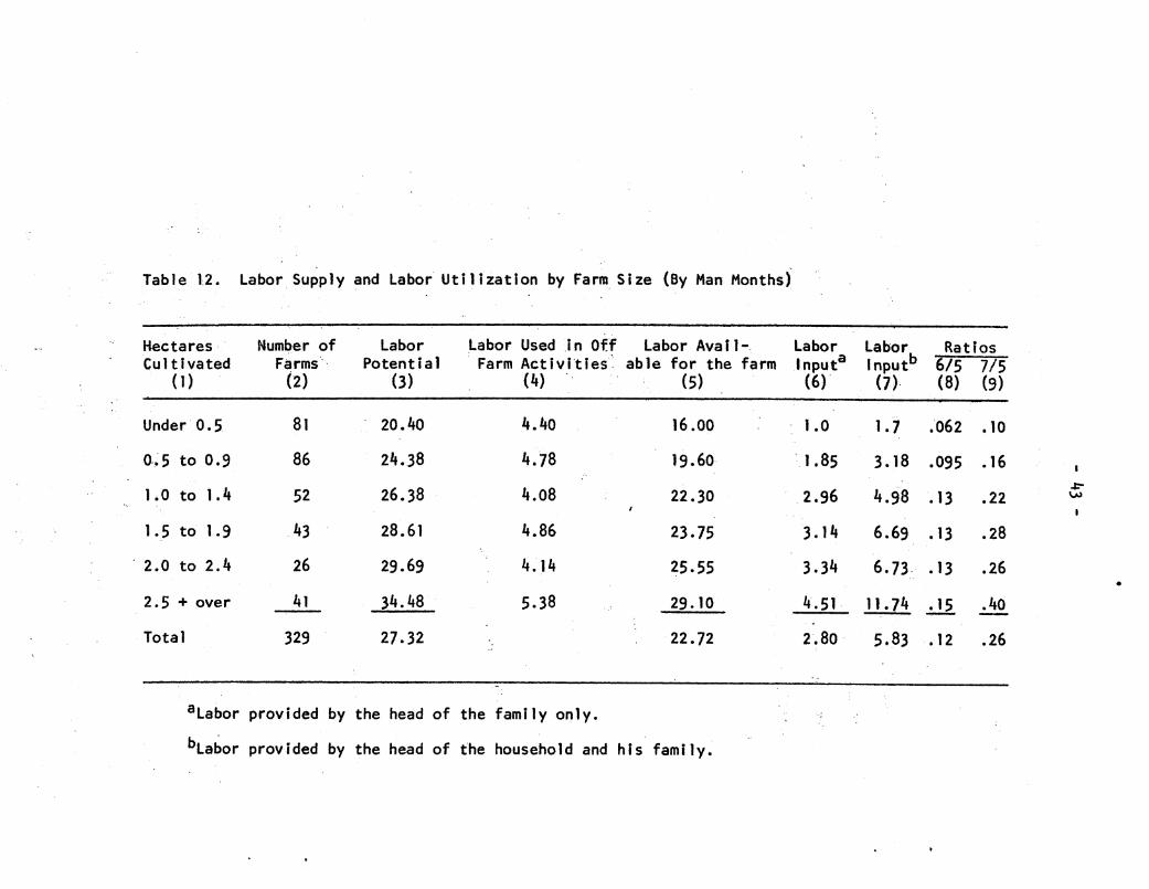
Labor Supply and Labor Utilization by Farm Size (By Man Months)
Hectares Number of Labor Labor Used in Off Labor Avail- Labor Labor RatiosCultivated Farms Potential Farm Activities able for the farm tnputa Inputb 6/5 7/5
(1) (2) (3) (4) (5) (6) (7) (8) (9)
Under 0.5 81 20.40 4.40 16.00 1.0 1.7 .062 .10
0.5 to 0.9 86 24.38 4.78 19.60 1.85 3.18 .095 .16
1.0 to 1.4 52 26.38 4.08 22.30 2.96 4.98 13 .22
1.5 to 1.9 43 28.61 4.86 23.75 3.14 6.69 .13 .28
2.0 to 2.4 26 29.69 4.14 25.55 3.34 6.73..13 .26
2.5 + over 41 34.48 5.38 29.10 4.51 11.74 .15 .40
Total 329 27.32 22.72 2.*80 5.83 .12 .26
aLabor provided by
bLabor provided by
the head of
the head of
the family only.
the household and his family.
Table 1:2.
I.l=-pa
I

- 44 -
recorded in the interview, or (c) the time that the farmers remained
unemployed.
In order to obtain data relating to labor units, each farmer
was asked how many man-days of labor were used in land preparation
and how land was prepared. He was asked about the labor inputs in
planting and cultivation, including the time spent on herbicidal
weed control and insect control with pesticides, harvesting,
threshing, shelling, and winnowing. This line of questioning was
repeated for each of the major crops--corn, frijoles, wheat and
potatoes.
By this procedure two estimates of the labor input on the
family farm were obtained--labor input of the head of the family
alone, and labor input of the head of household and his family
(see Table 12). These two estimates are a measure of the actual
farm labor input.
The remarkable difference between labor available and labor
input can be observed in Table 12.
On the average, labor input is 12 percent of labor available
when only the labor force of the head of the household is con-
sidered. The corresponding figure for the head of the household
and his family is 24 percent.
Table 12 shows that family labor used on the farms increased
from 1.70 man-months on holdings of under 0.5 hectares (average
0.27 hectares) to 11.74 man-months on farms of 2.5 hectares or
more. Of this, one man-month of the total 1.7 man-months was

- 45 -
supplied by the operator on the smallest farms; on the largest farms
the operator supplied 4.5 man-months.
Table 13 shows that the intensity of labor used on the farm does
not vary significantly among various departments, suggesting a high
degree of homogeneity among the peasants in the Guatemalan Highlands
regarding the use of labor in farm activities.
Table 13. Average Man-Months of Labor of the Operator and OtherFamily Workers in Production of Principal Crops byDepartments
Department
Chimal tenango
Toton i capan
Quezal tenango
Quiche
Solola
San Marcos
Huehuetenango
Total
AverageHa. PerFarm
1.41
0.64
2.06
1.00
1.11
2.46
1.74
1.49
AverageMan-MonthEmployeda
2.81
1.74
1.71
1.85
1.96
3.02
2.16
2.17c
AverageMan-MonthEmployedb
4.80
4.13
3.37
3.90
4.00
7.29
5.23
4.67C
aLabor provided by the head of the family only.
bLabor provided by the head of the household and his family.
CThe present average was calculated from 329 instead of 340
observations.

- 46 -
Mobilityiof the Highland Farmers
No great degree of mobility was found in the population. Among
sample households, 80.2 percent of the household heads were still
living in the communities of their birth, 18.4 percent in another
community but in the same department, and only 1.4 percent in other
departments.
In San Marcos 90 percent of the heads of families lived in the
communities of their birth. The corresponding figures for Solola
and Quiche were 91 and 94 percent, respectively, while in both
Quezaltenango and Huehuetenango the figure was 96 percent.
Family heads in the Department of Chimaltenango were the most
mobile: 56 percent still lived at their birthplace while 42 percent
lived in an adjoining municipio.
The immobility of the Highlands population can be further
demonstrated: the children and siblings of 76.7 percent of house-
hold heads still lived in the community of their birth at the time
of the interviews. In some departments, none of the adult children
have migrated from their home communities; and only 4.3 percent of
sample families reported that one or more of their adult children
had migrated. Most of the migration that occurred was accounted
for by siblings of the family head. The heaviest migration of
siblings, which occurred in Quezaltenango, can be explained by the
location of the area studied--less than three kilometers from the
capital city of this department. The migration rate of siblings
in the zther departments was much less than it was in Quezaltenango.

- 47 -
Capital Input
Land constitutes the main capital investment of the Guatemalan
Indian farmer. Taking the owners' estimates of current market values
for their land, buildings, livestock and tools, gives an average value
of Q1,370 per farm (see Table 14). Dividing the value of land alone
by the average area of farm (3 hectares), the average value of one
hectare of land in the study region is Q363.
Omitting the atypical department of Quezaltenango, the estimates
are reasonably uniform among departments, the difference between the
lowest and the highest values being only Q500, or about one-third the
average value. Two main factors influenced the variation.
One was the proximity of the Sample aldea to a large urban con-
centration; the sample community in Quezaltenango, less than three
kilometers from the capital of the department, clearly demonstrates
this factor's influence. This sample aldea is really a part-time
farming community where many of the farmers work in the factories,
commercial establishments and service industries of the city in the
morning, and tend their lands in the afternoon. Consequently, land
values are high. Rentals, for example, were found to be as high as
Q1.25 per cuerda per year for the best land, but since much of the
land is hilly and stony, prevailing rentals were around Q.0.75 per
cuerda (a cuerda varies in size depending on region, but officially
equals 0.044 hectares).
- 48 -
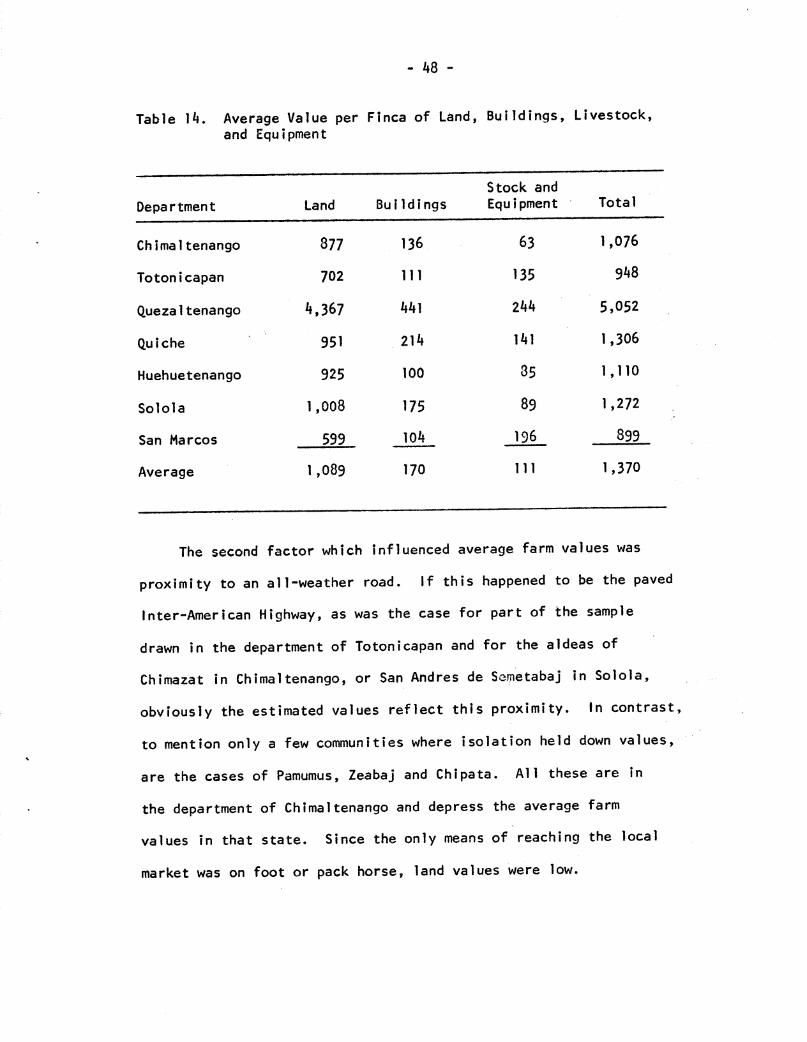
Table 14. Average Value per Finca of Land,and Equipment
Buildings, Livestock,
Stock and
Department Land Buildings Equipment Total
Chimaltenango 877 136 63 1,076
Totonicapan 702 111 135 948
Quezaltenango 4,367 441 244 5,052
Quiche 951 214 141 1,306
Huehuetenango 925 100 35 1,110
Solola 1,008 175 89 1,272
San Marcos 599 104 196 899
Average 1,089 170 111 1,370
The second factor which influenced average farm values was
proximity to an all-weather road. If this happened to be the paved
Inter-American Highway, as was the case for part of the sample
drawn in the department of Totonicapan and for the aldeas of
Chimazat in Chimaltenango, or San Andres de Semetabaj in Solola,
obviously the estimated values reflect this proximity. In contrast,
to mention only a few communities where isolation held down values,
are the cases of Pamumus, Zeabaj and Chipata. All these are in
the department of Chimaltenango and depress the average farm
values in that state. Since the only means of reaching the local
market was on foot or pack horse, land values were low.

- 49 -
Capital investment in stock and equipment was influenced by the
type of farming, with livestock the most influential component. Most
farmers owned a machete and hoe, and a few also possessed hand
sprayers and cross-cut saws. In the group composed of Totonicapan,
Quezaltenango, Quiche, and San Marcos, the average investment was
Q.179 per farm; in the group composed of the other three departments,
the average was Q.79, or about half as large. The higher figure for
Quezaltenango is caused by the presence of some fairly flocks of
sheep on some farms. Sheep were almost totally absent in
Chimal tenango.
Livestock population for the sample as a whole is small indeed.
Table 15 shows the number of head per livestock category.
Table 15. Livestock Population on Survey Farms
Number of Number of
Category Head Farms
Sheep 1,085 65
Cattle (dairy) 80 45
Fowl 2,668 290
Pigs 175 125

- 50 -
V. The Statistical Estimation of the Production Function
When estimating a production function one faces, among others,
the following problems: (1) the choice of the algebraic form of the
production function; (2) the kind of variables to be included in the
function and the units in which they should be measured; and (3) the
way in which the coefficients of the production function should be
estimated.
We chose the unrestricted Cobb-Douglas form of production func-
tion which is linear in the logarithms because of (1) its computa-
tional attractiveness, (2) its ease of interpretation, and most
importantly, (3) because it fits the data well. The coefficients
of the production function were estimated using the "least squares
regression techniques" applied to the logarithms of the variables.
As indicated in the preceding chapters, the difficulty of
obtaining information and the chances of making serious errors in
the specification, measurement, and aggregation of economic data
from traditional peasant agriculture are very great. Hence the
kind of variables included in the production function were largely
determined by the availability and reliability of the data. The
variables used and their units of measurement are described below.
The Production Function
The Cobb-Douglas product ion function fitted to our data can
be wri tten:
Y=AX b2 b3E-------- ()
1 X 2X3 E. . . . I
- 51 -
where Y is output; A is a constant; X is land; X Is labor; X is2 3
capital; bp, b2 and b are their respective production elasticity3
coefficients, and E is a stochastic term.
In its logarithmic form the Cobb-Douglas production function
can be written as
y + b x! + b2x2 + b3x3x+
where y log Y;Ac = log A; x1 = log X; x2 =log X2; x -log X ;2. .3 3
and b1 ,9b2 and b their respective regression coefficients.1 2 3
The Data
Output
Aggregate value of farm production is taken as a measure of
output. This aggregate value of farm production consists of the
value of the products sold plus an estimate for the value of farm
products consumed in the household. The most important crops are
corn and beans, which in most cases are cultivated in the same
field. Wheat is cultivated to a lesser extent on some farms.
Sometimes corn, beans, and potatoes are planted in the same field,
making the problem of desegregation of the value of agricultural
output and the use of a production function for each crop very
difficult. The output of each crop was weighted by the aviaje
price paid in the area.
• Input s
Land was measured in hectares and also in monetary terms.
There is reason to believe that land In the area under study is
- 52 -
fairly homogeneous in quality, in which case measurement in physical
units is a good approximation of land inputs. In some of the produc-
tion functions the estimated values of land, according to market
value, were used as land inputs in order to obviate the problem of
aggregating non-homogeneous land.
Labor inputs were provided mainly by the members of the family;
and were estimated by calculating the weighted contribution of each
family member according to his sex and age. In this manner labor
potential os the family was transformed into homogeneous man-month
units. The estimated man-months inputs were weighted by the average
wage rate prevailing in the area and hence transformed into monetary
labor units, and used in some of the calculated regressions.
Capital among the Guatemalan Highland Indians consists mainly
of very primitive farm implements like machetes and hoes. In the
unusual cases where cattle and horses were found, they were included
as part of the capital used in farm production. The problem of
adding non-homogeneous capital inputs was solved by substituting
capital values for physical capital. Themmarket value of agricul-
tural implements and live capital inputs at an undepreciated re-
placement cost was used as an index of capital inputs. However, the
use of capital stocks--either in physical terms or in monetary
values--generally does not provide the most appropriate estimate
of capital inputs to use in a production function. Capital inputs
must be introduced in terms of current service flows rather than
- 53
in terms of capital stocks. 17 The use of capital stocks instead of
capital flows in this case does not introduce a significant source
of error. The information obtained in the questionnaires indicates
that the life expectancy of the farm implements used by the Guatemalan
Highland farmers is seldom more than a year, the duration of the
production period. In this case the use of the value of capital
stock is a good approximation of the value of the flow of services
of that stock of capital for a given period of time. However, due
to the lack of more specific information about the appropriate rate
of discount and life expectancy of live capital, we did not estimate
the flow of services derived from live capital like horses or mules,
but used instead the stock value of them. However, the error
introduced for using this measurement of capital is thought to be
very small, since, as explained above, seldom were farmers found
who owned this kind of capital.
17Zvi Griliches, "Measuring Inputs in Agriculture, A CriticalSurvey," Journal of Farm Economics, Proceedings, Vol. 42, No. 5(December 1960), pp. 1411-33; Griliches, "Capital Stock inInvestment Functions: Some Problems of Concept of Measurement,"in Measurement in Economics, Studies in Mathematical Economicsand Econometrics (in memory of Yehuda Grunfeld) (Stanford,California: Stanford University Press, 1963), pp. 1153)7. Alsosee Pan A. Votopoulos, "From Stock to Flow Capital Inputs forAgricultural Production Functions: A Microanalytic Approach,"Journal of Farm Economics, Vol. 49, No. 2 (May 1967), pp. 476-91,and the discussion by Richard H. Day in the same volume.

- 54 -
Production Elasticities
Production elasticities indicate the changes in output relative
to changes in the inputs of the factors of production.
Table 16 shows production elasticities calculated for regres-
sions that include the total number of farms in the sample. Thus,
for RI.0, a one percent increase in the land input would lead to
a 0.71 percent increase in the total value of agricultural output.
An increase of one percent in the labor input would increase the
total value of agricultural production by 0.10 percent. An
increase of capital input, on the other hand, would Increase the
value of agricultural output by 0.18 percent. Similar interpreta-
tions can be given to the other coefficients.
The sum of the estimated production coefficients in a Cobb-
Douglas production function measures the phenomenon of returns to
scale. These data strongly suggest the presence of constant
returns to scale in the minifundia agriculture of the Guatemalan
Highlands. For the sample as a whole (see Table 16), one of the
sums of elasticities is significantly different from one at a
probability level < 1 percent.
Production functions were also estimated for each of the
departments studied. The land production elasticities coefficients
indicate that land is the most important factor of production.
The relative contribution of land to agricultural production
seems, however, to vary considerably among departments. The
relative contribution of labor and capital inputs to agricultural
production show less variation among departments than do land
inputs.

Table 16. Production Elasticities and Related Statistics
Regression
Item RI.O a RI.Ib R1.2c RI.3 a RI.4b Rl.5c RI.6a R1.7b
No. of Farms 340 330 330 340 330 330 340 330
R2 •869 .69 .69 •65 .65 .65 .69 .69
Elastici ties.71 .72 .76 .82 .80 .85 .77 .76
bI (land) (.04) (.04) (.03) (.04) (.05) (.03) (.03) (.03)
b2 (labor) .10 .04** .005"* .10 .08* *05*(.05) (.o4) (.05) (.05) (.o5) (.05)
b3 (capital) .18 .18 .18 .18 .18(.02) (.02) (.02) (.04) (.02)
Sum ofElasticities .99 .94 .94 .92 .88## .90 .95 .94
Non-starred coefficients are significantly different from zero at a probability level < 5%.*Starred coefficients are significantly different from zero at a probability level < 10%.
*Starred coefficients are not significantly different from zero at a probability level 1.
() Numbers in parentheses refer to the standard error of the regression coefficients.
aLabor inputs of head of family alone
bLabor inputs of head of household and his family.
cLabor inputs computed as the difference between total labor available and labor spent off
the farm.Sums with no ## symbol are not significantly different from one at a probability level <5%.
##Sums are significantly different from one at a probability level < I%.
I%.,
- 56 -
The sum of the elasticities coefficients in each department,
except in Totonicapan, suggests again the presence of constant returns
to scale in the agricultural enterprises of the Guatemalan Highland
Indians.
Marginal Value Productivities and Efficienc in the Use of Resources
Production elasticities indicate changes that take place in the
value of output when we change the level of a given input. Would
these changes increase the efficiency in the use of the factors of
production?
In order to answer this question an index of efficiency must be
found; this index is obtained by comparing the value of the marginal
product of a given resource to its opportunity cost. Maximum effi-
ciency occurs when the value of the marginal product of a resource
is equal to the unit cost of that resource. If the ratio of marginal
product to opportunity cost is more than one, it means that too
little of that resource is being used at a given price level. If
the ratio is less than one, too much of that resource is being
utilized. This criterion of maximum efficiency is valid, of course,
only when perfect competition exists in the resource and product
markets. It is further assumed that if the efficiency conditions
exist in all sectors of the economy, the economy is in a situation
of Pareto optimality. If disequilibria exist in the agricultural
sector, then a correction of these through a decrease or increase
in the use of the factors may (but not necessarily) lead to a
situation of Pareto optimality.

- 57 -
Hence, in order to obtain an index of efficiency in the use of
a given resource, there must be an estimate of that resource's
marginal productivity and its opportunity cost.
From the estimated production elasticities, one can obtain their
corresponding marginal productivities. The marginal productivity for
a resource X. is given by
Y b I YI
w x.
where Y is output, Xi a given resource and b the production elastic-
ity that corresponds to resource i, other factors of production being
held constant. Marginal productivities can be computed at any com-
bination of input and output levels that lie within the range of the
sample observations. All the estimated marginal productivities were
estimated at the geometric mean levels of inputs and outputs. The
use of the geometric (rather than the arithmetic) mean levels seems
more appropriate within the context of a Cobb-Douglas production
function.
As a measure of the opportunity cost of one unit of land, we
took the average land rent of a unit of land in the area. The
average monthly salary earned by a farm laborer was taken as the
opportunity cost of one man-month unit of labor. The opportunity
cost of capital was more difficult to determine. No organized
financial market exists in the area and the rates of interest
charged by local money lenders vary greatly among villages and depart-
ments. In some cases, money lenders charge different rates of

- 58 -
interest to different customers. The estimated opportunity cost of
capital is an average of the different rates of interest on loans as
recorded in the interviews.
Marginal Productivity of Land
Since the estimated marginal productivities were calculated at
the geometric mean of the variables Y and X. they relate to the
"average geometric farm"--whatever that means.
The estimated marginal productivities for land, for the sample as
a whole, using different kinds of labor inputs and different units of
measurement for land and labor inputs, are given in Table 17. The
estimated marginal productivity of land ranges from Q 86.80 to
Q 103.00 per hectare of land. But even if the productivity of land
is as high as Q 103.00 per hectare, it is not possible for farmers
to bring more land under cultivation, since most of them use all
the cultivable land they control.
Marginal Products Estimated at the Sample Means and Efficiency Ratios
Rcoiress ionI tem RI.0 RI.1 RI .2 R!J.3 R1.4 R1.5 Rl.6 R1.7
Sample Geometric Means
Output (#)Land (Ha) and ($)Labor (Man-month) and ($)Capital ($)
Marginal Products(at Geometric Means)
Land ($/Ha)Labor ($/Man-month)Capital ($/$)
Marginal Return toOpportunity Cost Ratio
LandLaborCap i taI
110.000.901.84
50.00
86.806.00
.40
5.5.51
1.25
110.00
0.903.1649.50
110.00
0.9017.5049.50
110.0000.901.84
49.50
88.00 92.90 100.00- - 6.00.40 .40 -
5.6.m
1.25
5.9
1 .25
6.3.51
A dash (-) indicates that production elmarginal productivities were not calculated.
asticities were not significant and hence the corresponding
I 10.000.903.16
49.50
110.000.90
17.5049.50
110.000.901 .84
50.00
110.000.903.1649.50
%I1
97.802.80
6.2.24
103.00
6.5
94.10
.40
5.9
1 .25
92.90
.40
5.8
1 .25
Table 17.
Table 18. Marginal Productivities at Different Input Levels for Selected Regressions
At BlwteMaAbove the Mean the Below the MeaInput Regression +50%+20%. + IO • Mean -0% . .20%
Land R1.0 78.40 82.60 84.50 86.80 89.60 93.10 112.0
(1.35) (1,08) ( .99) (0.90)( .81) ( .72) (.4s)RI.3 94.O0 97.00 98.40 100.80 132.00 104.50 118.0
(1.35) (1.08) ( .99) ( .90) ( .81) ( .72) (145)
R1.4 91.30 94.50 96.00 97.80 100.00 102.70 117.40(1.35) (1.08) (.99) (.90) (.81) (.72) (.4s)
Labor RI.0 4.20 5.10 5.50 6.O0 6.60 7.30 11.14(2.76) (2.20) (2.02) (1.84) (1.65) (1.47) (.92)
R).3 4.20 5.10 5.50 6.00 6.60 7.30 11.14(2.76) (2.20) (2.02) (1.84) (1.65) (1.47) (.92) o
RI.4 1.90 2.40 2.60 2.80 3.14 3.45 5.40(4.70) (3.80) (3.48) (3.16) (2.85) (2.50) (1.60)
Capital RI.0 .29 .34 .37 .40 .44 .48 .73(75.00) (60.00) (55.00) (5o.00) (45.00) (4o.oo) (25.00)
Numbers in parentheses are the corresponding input levels above and below the geometric means.
- 61 -
Table 18 gives the marginal product of land at different input
levels for regressions R1.O, RI.4, RI.5 and Figure 1 plots their18
corresponding product lvi ty curves.
The average opportunity cost of one hectare of land for the
sample as a whole was estimated to be Q 15.80. The efficiency ratios
as measured by the ratios of the marginal productivity of land to its
opportunity cost vary from 5.5 to 6.5, and indicate that farmers are
18The relevant estimates of the marginal productivities were made
in the following way (See Pan A. Yotopoulos, Allocative EfficiencEconomic Development, Athens: Center of Planning and Economic Research,1967, p. 199):
We know that the marginal productivity of resource X. is given by
.3 i i
where Y is the output and Xi the Ith input and be the production
elasticity of resource i. By letting m denote the value of themarginal product, we can rewrite the above equation as
in =b Y
For an input level of 10 percent above the mean, we can write
m+]0 =b i I + JlObi Y
x.
Since m bi hence we have
_mM + .l b
m+10 =m10
A similar method was used to estimate marginal productivities atdifferent input levels.

Figure 1. Marginal Productivity of Land, Regressions R1.0, RI.4, R1.3
Marginal Productivity ($/Ha.)
1 130
125
120
115
_110
105
100
90 R1.4
~80_8o -- ...
75 " R i .0
70
-80 -70 -60 -50 -40 -30 -20 -10Land Input (Ha.) Mean
+10 +20 +30 +40 +50 +60 +70 +80Land Input (Ha.)
I

- 63 -
using too little land inputs. However, land shortages and institutional
constraints Imposed on the farmers limit their ability to use more land
inputs in their farm activities. The consequences of this situation
and its policy implications are discussed in the next section.
Marginal Productivity of Labor
The estimated marginal productivities of labor for the regressions
of the sample as a whole are given in Table 17. Among the regressions
computed, the marginal productivity of one man-month unit of labor
ranges from Q 2.80 to Q 6.00. Table 18 shows the marginal productivities
for regressions R1.0 and R1.4, and Figure 2 plots their productivity
curves.
How does the marginal product of labor compare to its opportunity
cost? A lack of data regarding employment opportunities prevented
estimation of the year-round level of unemployment among the Guatemalan
Highland farmers, and hence estimation of the true year-round opportunity
cost of labor. However, three different estimates of the opportunity
cost of labor were made in order to compare them to the marginal produc-
tivity of labor in the area. The average of these three estimates was
used for calculating the efficiency indexes for the sample as a whole,
shown in Table 17.
The three estimates of the opportunity cost of labor are the
following:
(1) The average wage rate for the area as a whole, as recorded in
the questionnaires, was Q.0.50 per day. Assuming that labor is fairly
homogeneous (a reasonable assumption since no great differences were

Postulated,-;Opportun i tyCost of Labc
Figure 2. Marginal Productivity of Labor, Regressions R1.0, RJ.4
Marginal Productivity ($/Man-Month)and Monthly Wage Rates
45
40
35
30
25
20
15
.10--------------------------.-Average..Market Wage
RateRI .0)r R1 0
-80 -70 -60 -50 -40 -30 -20 -10MeanLabor Input (Man-Month)
+10 +20 +30 +40 +50 +60 +70 +80
Labor Input (Man-Month)
0%

- 65-
found in education and special skills among farmers) and that the
daily wage rate does not vary during the year, the average monthly
(26 days) salary came to Q. 13.00. This monthly salary was taken as a
proxy for the opportunity cost of one man-month of labor in the area
as a whole. Using this figure, the ratio of the marginal productivity
of labor to its opportunity cost was found to be significantly below
unity for all regressions. This suggests that when the opportunity
cost of labor is calculated to be Q 13.00, our findings indicate in-
efficiencies in the use of family labor inputs by the Guatemalan
Indian farmers. Too much labor is being used in the production process.
(2) if, on the average, the Highland farmers spend about three
months of the year in the Lowlands of the country as migrant workers
and make an average of Q 0.88 a day; and if for the rest of the year
they can earn Q 0.50 a day working in the Highlands as farm laborers
and at miscellaneous activities, then the estimate of the opportunity
cost of one man-month of labor can be set at Q 15.50. WIth this
estimate of the-opportunity cost of labor, the ra:itio of rar-yinal
product of labor to its opportunity cost is, as ve, ov, es tP.hnn one
for all regressions. This result agaiin s,,',e;ts, that, aivY,2n. the op-
portunity cost of labor, too much 1abor is being put into farm activ-
ities by the Guatemalan Highland ihidians.
(3) If the opportunity cost of labor is zero for the seven months
a year that the farmers neither work in the Lowlands as mi.grant
workers nor as self-employed farmers, then a different estimate of
the year-round opportunity cost of labor results. This approach
would probably capture the seasonal unemployment during which surplus
- 66 -
labor might exist. Weighing the monthly wage rate of Q 15.50 by the
proportion of the year in which the opportunity cost of labor is
zero, a year-round monthly opportunity cost of labor of Q 6.45 is
obtained. With this new estimate of the monthly opportunity cost
of labor, an efficiency index very close to unity results (except
for regression RI.5, which includes the labor inputs of the head
of the household and his family). This approach would suggest that
Guatemalan Indian farmers are using their family labor force in
farm activities up to a nearly optimum level.
However, when the average of the three estimates (Q 11.65)
is taken as the opportunity cost of one man-month of labor (see
Table 17), one may observe, on the whole, indications of inefficient
use of family labor among Guatemalan Highland Indians. The effi-
ciency indexes suggest that too much family labor is being used
in farm activities.
Little can be said about the marginal productivity of labor
in each department. Most of the elasticity coefficients for labor
were not significant and hence the respective productivities were
not calculated.
Marginal Productivity of Capital
The estimated marginal productivities of capital inputs for
the sample as a whole are shown in Table 17. The marginal produc-
tivity of capital was o.40 for all regressions. The marginal
productivity of capital is a pure number, since it is expressed
in Quetzales of output per Quetzales of capital; this number

- 67 -
expresses the increment of output in Quetzales with the use of one
additional Quetzal of capital input. If capital inputs are measured
in flow of capital services rather than in capital stocks, then this
number cannot be directly compared with the opportunity cost of
capital as measured by the rate of interest.19 However, since
capital inputs in the production function were measured as stocks of
capital, we can meaningfully compare the marginal productivity of
capital with the opportunity cost of capital as measured by the rate
of interest.
According to the data collected in our questionnaires, several
market rates of interest prevail in the area under study. Of al
the farmers interviewed, the small number (19 percent) who had
obtained an average annual credit of Q 16.00 obtained this credit
at interest rates varying from 8 percent a year up to 60 percent a
year. Based on these rates of interest, the average opportunity
cost of one Quetzal of credit for agriculture is estimated at 32
percent.
The ratio of the marginal product of capital to its opportunity
cost for the regressions of the sample as a whole are given in
Table 17. The efficiency ratios greater than one, indicate ineffi-
cient use of capital inputs among Guatemalan Highland farmers.
The observed differences in marginal productivities among
departments suggest the possibility of increasing agricultural
output by reallocating existing capital resources among departments.
19yotopoulos (1967), op. cit., p. 206.

- 68 -
The Optimum Level of Inputs
From the computed marginal productivities we can obtain the
quantity, with other inputs held at their mean levels, necessary to
equate the marginal productivity of a factor to its opportunity
cost,
When land, labor and capital are included, our Cobb-Douglas
production function is written as:
Y = A Xb1 Xb2X 3 (1)
where Y is output; A is a constant; X is land; X2 is labor; X3 is
capital, and b1, b2 , b3 are the corresponding production elasticities.
In order to find the level of, for example, input X2 at which
the marginal product of that input is equal to its opportunity cost,
the first derivative or marginal product of (1) is set equal to the
opportunity cost of X2:
X P ~ 2 b -12 _2(2)
Ab 2 X 1X3
where P2 is the opportunity cost of factor X2 and X,, X3 the geo-
metric means of inputs XI X3 . A similar procedure applies in
finding the optimum levels of other inputs.
For the sample as a whole, the estimated level of labor input
at which the marginal productivity of labor equals the postulated
opportunity cost of Q 6.35 is 1.55 man-months for regress ion Rl.O
and 1. 19 man-months for regression Rl .5. I f the average market

- 69 -
wage rate of Q 11.65 is used, the optimum level of labor inputs for
the sample as a whole is only 0.85 man-month for regression Rl.O.
On the other hand, for the sample as a whole the actual average
level of labor Inputs used by the Guatemalan farmers was 1.83 man-
months in regression RI.O (including the labor force of head of house-
hold only) and 3.16 man-months in regression RI.5 (including labor
force of head of household and his family). Hence, according to the
estimated optimum levels of labor Inputs, Guatemalan Highland farmers
must reduce family labor inputs by 16 percent according to regression
RI.O and by 63 percent according to regression R1.5, when the
estimated opportunity cost of one man-month of labor in the area is
Q-6.35. If, however, the true opportunity cost of one man-month of
labor is Q.11.65, farmers must reduce their family labor inputs by 53
percent according to regression RI.O. A graphic solution to the
problem of finding optimum labor Input levels is shown in Figure 2,
which is based on Table 18.
A word of caution Is needed about the method of estimating
marginal productivities and optimum input levels. The extrapolation
of the marginal productivity values above and below the mean input
values becomes less and less reliable as we move away from the mean
of the range observed. Hence, even if, as in this case, the estimated
optimum input levels fall well within the range of observations, the
results should be interpreted with caution.
When equation was applied (2) to find the optimum levels of land
inputs, we obtained less satisfactory results than in the case of

" 70 s
labor. If Q 15.80 is a good approximation of the opportunity cost of
one hectare of land, the optimum level of land inputs for the average
Guatemalan Highland farmer was estimated at 269 hectares in regression
RI.O and 5,937 hectares in regression R1.5.
On the other hand, the actual average level of land inputs for
the sample as a whole is 0.9 hectares for both regressions. This
means that, given the marginal productivity of land and its prevalent
opportunity cost, farmers should, in order to make efficient use of
land, increase the area under cultivation from less than one hectare
to about 269 hectares according to regression RI.O and to about
5,937 hectares according to regression R1.5. The estimated necessary
land input increases are highly unrealistic for the type of agri-
culture under consideration.
The unrealistic results obtained regarding the optimum level of
land inputs point out the limitations of this kind of analysis and
of the use of Cobb-Douglas production functions in the study of
traditional agriculture. The optimum levels of land inputs
estimated by equation (2) are sensitive to changes in the opportunity
cost of land and particularly to the size of the land production
elasticity coefficient. Larger values for the opportunity cost of
land and smaller land production elasticity coefficients give
smaller (more realistic) optimum levels of land inputs.
Table 19 shows the estimates of the optimum levels of land and
labor inputs for regression RI.5 holding the opportunity cost of
land (Q 15.80) and labor (q 11.65) constant but varying
simultaneously the size of their respective production elasticity
coefficients.

- 71 -
Table 19. Optimum Levels of Land and Labor Inputs in Regression Rl.5when Varying their- Production Coefficients and theOpportunity Cost of Land8
Production Elasticity Coefficients
I II III IV V
Input bl0 80 bi= .70 b 1 .60 b1= .50 b| =
b2= .08 b2 . 18 b2= .28 b2w .38 b2= .48
x (land inhectares) 5,937 339 82 27 12
(255) (54) (16) (9) (8.7)
X2 (labor inman-month) .66 1.68 3.41 8.5 15.4
'Figures in parentheses refer to the optimum levels of land in-
puts when the elasticity coefficients were varied and the opportunitycost of land was doubled from Q15.80 to Q31.60. The other numbersrefer to the optimum Input levels estimated when only the productionelasticity coefficients were varied, holding the opportunity cost ofland and labor constant at Q 15.80 and Q 11.65 respectively.
The effect that small changes in the size of the land elasticity
coefficient have on the level of land Inputs needed to achieve
optimum efficiency Is remarkable. A reduction of about 13 percent
(from 0.80 to 0.70) in the size-of the land elasticity coefficient
brings about a reduction in the optimum level of land input of about
96 percent (from 5,937 hectares to 339 hectares). Further reductions
in the size of the land production elasticity coefficients, accompanied
by similar increases in the size of labor coefficients (111, IV and
V in Table 19) have less dramatic impact on the estimated optimum
land Input levels.

- 72 -
The effect that a simultaneous increase in the labor coefficients
and reduction in the land coefficients have on the optimum level of
labor inputs are less marked than the effects that similar changes
have on the optimum level of land inputs (see Table 19). An increase
of 125 percent (from 0.08 to 0.18) in the size of the labor coefficient
increases the level of labor inputs needed to achieve efficiency by
154 percent (from 0.66 man-month to 1.68 man-months).
The use of different estimates of the opportunity cost of land
also affects the equilibrium levels of land inputs. A doubling of
the value of the opportunity cost of land (from Q 15.80 to Q 31.60)
reduces the optimum level of land inputs by about 94 percent (from
5,937 hectares to 255 hectares). This reduction to 255 hectares in
the optimum level of land inputs is very close to the 236 hectares
(not shown in Table 19) obtained when the land coefficient is
reduced by 13 percent (from 0.80 to 0.70) without simultaneously
increasing the labor coefficient, as is done in 11. The important
point to notice here, however, is that these very similar results
were obtained in one instance by increasing the value of the
opportunity cost of land by 100 percent and in the second case by
only reducing by 13 percent the size of the land coefficient.
The function used to estimate the optimum levels of land input
seem to be far more sensitive to variations in the size of the
land production elasticities than to changes in the value of the
opportunity cost of land.
/lhen we increase the opportunity cost of land and simulta-
neously reduce the size of the land coefficient (see figures in

- 73 -
parentheses in Table 19), the optimum levels of land inputs come out
considerably lower than when only the production coefficients are
varied (see figures without parentheses in Table 19).
The use of equation (2), as by Heady and Dillon20 and Yotopoulos, 2
1
might, as shown above, lead to serious errors when predicting optimum
levels of resource use. The over-sensitiveness of equation (2) to
variations in the size of the production elasticity coefficients
imposes serious limitations on its use. Specifically, (2) might yield
extremely large optimum values for a given input when that input is
considerably more important than the other inputs in the production
process. In other words, unrealistic optimum values for a given input
are obtained when the production elasticity coefficient of that input
is very large--say above 0.5--as compared with the elasticity coeffi-
cients of the other inputs accounted in the production function.
Unfortunately this is the case for the traditional agriculture of the
Guatemalan Highlands. Land, as suggested by the size of the land
production elasticity coefficients, is by far the most influential
input, with labor and capital playing a secondary, although
statistically significant, role.
2 0 Earl 0. Heady and John L. Dillon, Agricultural ProductionFunction (Iowa State University, 1962), p. 631.
2 1yotopoulos (1967), OP i. p. 199.
- 74 -
Comparison with Studies Made in Other Countries
Table 20 displays the results of several cross-sectional produc-
tion functions of farms around the world. All these studies are
based on Cobb-Douglas, single equation models. All non-land and non-
labor inputs were collapsed in the "other services" category, because
of the lack of agreement on the definition of capital among the
various studies.
The elasticity coefficients, and the ratios of marginal product
to opportunity costs are indicated in Table 20. These ratios, as
explained, provide a measure of the efficiency in the use of
resources.
The estimated annual rent of one unit of land is taken in all
studies as a proxy of the opportunity cost of land. The market wage
rate was considered a good approximation for the opportunity cost
of labor. The opportunity cost of a monetary unit of capital was
estimated as that monetary unit plus the annual cost of borrowing
it.
The sum of the elasticities of the factors of production in
most cases is one, or very close to one, indicating the remarkable
fact that, according to the studies made, world agriculture is
characterized by constant returns to scale.

75 -
As indicated above, an efficiency ratio of less (or greater)
than one indicates that too much (or too little) of a given resource
is being utilized. The less than one efficiency indexes in most
of the countries, but particularly in India and Guatemala, indicate
marked inefficiencies in the use of agricultural resources.
Table 20. Production Elasticities and Ratio of Marginal Product to Opportunity Costfor Selected Cross-Sectional Production Function Studies
Ratio of Marginala Product to
Elasticity of Productiona Opr UOpprotuni ty CostLocation of Type of Other OtherSample Farming Labor Land Services Sum Labor Land Services Reference
Mixed
Generalarable land
Mixed
.10 .77 .18 1.05
.56 .08 .25
.44 .10 .11
.89
.65
.51 5.5 1.25
n.a. n.a. n.a.
.87 .90 .91
Present study (1968)
Sarker (1957)
0%
Yotopoulos (1967) o
India, UttarPradesh
Wheat,sugar cane o43 .23 .35 1.01 .68 .95 2.13 Agrawal and Foreman
(1959)
,60 .93 n.a.
•33 .44 .31 1.08 2.84 .58
n.a.
.99
.32 .39 .46 1.17 .38 4.01 1.01
Heady (1952)
Wang (1959)
Heady and Sbaw(1954)
Guatemala
India
Greece,Epi rus
U.S.A.
TaiwanTa i nan
U.S.A.A I abama
.33Crop
Cereals
Crops

.26
.26
.12
.14
.13
-. 01
.13
.61
.67
.20 .39 .34
.53
1 .00
.78
.21
.54
.86
.05
.92
n.a.
•93 1.21 2.58
.35
1.501.09
1 .01
India,AndhraPradesh
Austria
Israel
Canada,Alberta
Inter-national
Inter-national
Agrawal and Foreman(1959)
Tintner (1958)
Mundlak (1964)
Darcovich (1958)
Bhattacharjee(1955)
Tinbergen andPelak (1950)
aFor all functions the elasticities are significantly different from zero at a probabilitylevel 5 percent. The only exception is the elasticity of land for the Israel function.
Source: Pan A. Yotopoulus, Allocative Efficiency and Economic Development (Athens: Centerof Economic Planning, Research Monograph Series, 1967), p. 212.
,28 .39 .33 1.00 n.a. n.a. n.a.
.70 .10 .20 1.00 na. n.a. n.a.
M i xed
M i xed
Mixed
Wheat,beef
General
(Hypothe-si zed)
- 78 -
V1. Surplus Labor, Disguised Unemployment,
and the Marginal Productivity of Labor
The findings so far presented offer insight into some issues
of development economics and provide grounds on which to outline
policy recommendations for the traditional sector of Guatemalan
agriculture.
As explained in Section II, one of the most important differ-
ences between the Classical (Lewis, Ranis and Fei, etc.) and Neo-
classical (Jorgenson, Schultz, etc.) theories of economic growth
is their assumption about the marginal productivity of labor in
the traditional sector of a dual economy. The Classical approach
maintains that after a certain level, labor in the traditional
sector becomes redundant with a marginal productivity of zero or
negative. This situation is characterized as "disguised
unemployment." On the other hand, the Neoclassical approach
maintains that labor in the traditional sector is never redundant.
That is, the marginal productivity of the agricultural sector is
assumed always to be positive and thus no "disguised unemployment"I
exists in the traditional sector of a dual economy.
This study's statistical findings bring some evidence to
this controversy. However, before discussing this problem, this
section will attempt to define more precisely the meaning of
"d isgu ised unemployment ."
The concept of " disguised unemployment" ' is sometimes
identified with one of the several interpretations given to a

- 79 -
surplus or excess supply of labor. The literature reveals at least
seven different interpretations of excess supply of labor.22 An
excess supply of labor is said to exist when:
(a) A low output per worker ratio is found in a region or
country.
(b) Output can be produced with fewer workers if factors of
production are recombined. Marginal productivity of labor is, in
this case, thought to be positive although probably very low.
(c) The same output can be produced with fewer workers, the
quantlity of other resources remaining unchanged--equivalent to
marginal productivity of labor equalling zero.
(d) Workers are seasonally employed.
(e) Workers are unemployed.
(f) "Too many" workers are In one sector so that wages are
lower for a certain class of employment in some sectors than in
others.
(g) The marginal productivity of labor is positive but less
23than the average product.
22Simon Rottenberg, "The Meaning of 'Excess Supply of Labor,"'Scottish Journal of Political Economy (February 1961). A modifiedversion of his classification is used here.
2 3Ranis and Fei call "disguised unemployment" that situationwhere the marginal productivity of labor is less than the averageproduct. On the other hand, they call "redundant labor" thatsituation in which the marginal productivity is zero (see c above).See Ranis and Fei, "'A Theory of Economic Development,", Amer icanEconomi c Revimew (September 1961|), p. 537.

- 80 -
If disguised unemployment means that situation of surplus labor
in which the marginal productivity of labor, although very low, is
positive (interpretations b and g above), then the present findings
are at least consistent with these interpretations. The size of the
elasticity coefficient of land relative to those of labor indicates
that Guatemalan agriculture is land and not labor intensive. On
theoretical grounds one expects to find the highest values of
elasticity coefficients for the factor that is used more intensively.2
4
Hence labor intensive agriculture must show labor elasticity co-
efficients higher than those for land. In this type of agriculture
it is expected that labor would be used at levels which yield large
additions to agricultural output. Hence high labor elasticity
coefficients which indicate labor intensive agriculture are incon-
sistent with the hypothesis of disguised unemployment which maintains
the existence of labor working but adding little to output. Under
conditions of labor intensive agriculture (shown by high labor
elasticity coefficients relative to land), labor is not redundant;
it is necessary in producing a given output, and cannot be removed
without decreasing the volume of agricultural output.
On the other hand, land intensive agriculture would be
characterized by land elasticity coefficients higher than those
for labor. Under this type of agriculture land is expected to be
used at levels that yield large additions to agricultural output,
24Y~otpu1us (1967), op. cit., pp. 215-216; and Heady and
Dillon, op. cit., p. 631.
- 81 -
and labor to be used at levels yielding only small additions to out-
put. Land intensive agriculture is then consistent with the exis-
tence of a situation in which labor adds little to output--disguised
unemployment.
In all regressions given here the estimated elasticity coeffi-
cients for land are higher than those for labor, indicating the land
intensive character of Guatemalan Highland agriculture. Since land
intensive agriculture is consistent with the existence of disguised
unemployment, as defined above, these findings suggest that at least
one of the necessary conditions for the existence of disguised un-
employment is present in the Guatemalan Highlands. Furthermore, the
marginal productivity of labor was found to be positive (see Table
21). These data then bring evidence to support the hypothesis of
disguised unemployment when defined as in b and g above. It is
important to notice that although the marginal productivity of labor
is positive, it is considerably smaller than the average wage rate
in the area., As shown in Table 17, the marginal productivity of
labor of the head of the household for the sample as a wihole was
estimated at Q 6.00, and the average postulated wage rate at Q 11.65.
Thus the marginal productivity of labor in the area is only about 51
percent of the average wage rate.
The existence of surplus labor identified with the marginal
productivity of labor being zero (c above) has been discussed by

- 82 -
,,25Nurkse, Lewis, Georgescue-Rogen and Ranis and Fei, among others;
in this form it has been attacked by Haberler, Viner, Shultz,
Jorgenson, and others.2 6
It is clear that our findings do not bring direct evidence
as to whether or not surplus labor (defined as that situation
where the marginal productivity of labor is zero) exists in the
Guatemalan Highland traditional agriculture. When we use a
Cobb-Douglas production function we implicitly assume that the
marginal productivity of labor is not zero. The mathematical
properties of the function are such that its first partial
derivative does not intersect (but approaches asymtotically)
the axes. Hence the marginal productivities, estimated using
a Cobb-Douglas production function, are either positive
25R. Nurkse, Problems of Capital Formation in Underdeveloped
Countries (Oxford: Basil Blackwe l, 1953 4 ; . A. Lewis, "Economic
Development with Unlimited Supplies of Labor," Manchester School
of Economic and Social Studies (May 1954); N. Georgescue-Rogen,
"Economic Theory and Agrarian Reforms," Oxford Economic Papers
(February 1960); G. Ranis and J C. H Foi,DvcI"Psment of the
Labour Surplus Economy: Theory and Policy (Homewood, Illinois:
Richard D. Irwin, Inc.,-t964),
26G. Haberler, "Critical Observations on Some Current Notions
in the Theory of Economic Development," L'Industria, Vol. II
(i195A, J. Viner, "Some Reflections on the Concept of 'Disguised
Unemployment,"' in G. Meier, Leading Issues in Development
Economics (New York: Oxford University Press, 1964); T. W.Schultz, Transforming Traditional Agriculture (New Haven, Conn.:Yale UniversTit 7rs,1964) Jorgensen (196l, 1966, 1967),
op. cit.

- 83 "
(when the production coefficients are positive) or negative (when the
production elasticities are negative), but they are never zero.
Incidentally, the same restriction occurs in a C. E. S. production
function27 with positive elasticity of substitution, since the marginal28
product of labor in this function never falls to zero either.
Therefore, we could not have tested the hypothesis that the marginal
productivity of labor is zero by fitting a Cobb-Douglas production
function to our cross sectional data.
On the other hand, negative marginal productivities for labor
can be shown to exist by fitting a Cobb-Douglas production function
to cross sectional data. This study did not find the marginal produc-
tivity of labor to be negative in the Guatemalan Highlands. For the
regressions of the sample as a whole, none of the estimated elastici-
ties are negative (see Table 16). Only a few of the regression
coefficients estimated in each department were negative, and none of
them were statistically significant. Therefore, these findings do
not support the hypothesis of disguised unemployment (defined as that
situation where the marginal productivity of labor is negative) in
the traditional agriculture of the Guatemalan Highlands.
2 7 K. J. Arrow, i1. 1 . Chenery, B. S. Minhas, and R. M. Solow,"'Capital-Labour Substitution and Economic Efficiency," Review ofEconomics and Statistics, Vol. 63 (1961).
28Amartya K. Sen, "Peasants and Dual ism W!ith or W4ithout a
Surplus Labor," The Journal of Political Economy (October 1966),p. 432.

- 84 -
Summarizing, then, these data support the hypothesis that the
marginal productivity of labor is positive. These results, however,
were obtained by a method that allows the estimated marginal
productivities to be either positive or negative but not zero.
This imposes certain restrictions on the results.
Does the existence of labor with positive marginal productivity
imply that there is no surplus labor? In a recent paper it has been
argued that "'the assumption of zero marginal productivity is neither
a necessary nor a sufficient condition for the existence of surplus
labor.'29 If true this statement implies that even if the marginal
productivity of labor was found to be different from zero, it does
not follow that there is no surplus labor. A situation of surplus
labor is consistent with the existence of positive, zero, or
neqative marginal productivity of labor.
If positive marginal productivity of labor does not conflict
with a situation of surplus labor, what other indications about
the existence of surplus labor can be found in our study?
Table 12 shows estimated labor potential (the weighted con-
tribution of each family member measured in man-month units) and
also the labor available for farm activities (man-month units
obtained by subtracting from the labor potential figure the
number of man-months employed in off-farm activities) in each
household. Table 12 also estimated the labor inputs of the head
of the family alone and of the head of the household and his
family to the family farm.
29Sen, op. cit.
- 85 -
if we add to the number of man-month units employed in off-farm
activities the number of man-months used in farm activities, this
figure estimates the number of man-month units that family labor was
employed. Hence the average household in the Guatemalan Highlands,
which has a labor potential of 27.3 man-months, actually uses only
10.4 man-months (man-months employed off farm activities plus labor
input'Iused on the farm), or about 38 percent of the total labor
potential. Household labor is thus employed only about 4.5 months
of the year.
Similar estimates can find the year-round level of employment of
the head of the household alone. Table 12 indicates that the average
farmer in the Guatemalan Highlands uses about 2.8 months per year
working on his farm. Adding to this figure the average three months (not
shown in Table 12) that he spends in the Lowlands as a migrant worker
or working in the community, we obtain 5.8 months. Notice that we
did not add to the man-month figure of 2.8 the difference between
labor potential and labor available, since this difference refers to
the off-farm work of all the family and not to the head of the
household alone.
Accordingly, the average farmer in the Guatemalan Highlands is
employed on his farm, as a salaried farm laborer, or as a migrant
worker only 5.8 months a year.
This study found in the Guatemalan Highlands substantial evidence
of a situation of surplus labor in which the marginal productivity of
labor is positive, and considerably smaller than the average wage rate
that prevails in the area. Regarding the Classical versus Neoclassical

- 86 -
controversy, the findings support the Neoclassical thesis that the
marginal productivity of labor in the traditional sector of a dual
economy is positive. However, the strongest Neoclassical position--
that because labor has a positive marginal productivity, labor is
never redundant--is not supported by these data.30 There was
evidence of excess or redundant labor (with a positive marginal
productivity) in the traditional agriculture of the Guatemalan
Highlands. On the other hand, the Classical argument--that there
is a point in the second phase of development after which the
marginal productivity of labor is positive but less than the wage
rate--is supported by our findings.31
30 See Jorgenson (1966), op. ci t., p. 46.
3 1 See Ran is and Fei (1961), op. cit., p. 537.

- 87 -
VII. Efficiency, Poverty and Economic Development
The basic problem of economic development lies in the creation
of an agricultural surplus that can be used to initiate the process
of industrialization.
The problem of creating an agricultural surplus can be approached
through the demand and/or supply sides.
Given the production function and the existing allocation of
agricultural resources, an agricultural surplus can be obtained by
reducing the level of consumption of the agricultural population,
i.e., through taxation, which can be compulsory (forced delivery of
goods to the non-agricultural sector), or non-compulsory (through a
policy of low agricultural prices).
The problem of creating an agricultural surplus is tackled from
the supply side by emphasizing the role of production instead of
consumption. The problem of creating an agricultural surplus,
according to this approach, can be solved through increasing produc-
tion by improving the efficiency of the use of agricultural resources.
Two variants of the "improving efficiency approachcan be
distinguished. 32
The first version has been called "the allocative efficiency
approach." In its orthodox, static form, it concentrates on marginal
32For the distinction between allocative and structural effi-
ciency, see: lila M yint, "Economic Theory and the UnderdevelopedCountries," Journl of olitical Economy, Vol. 73, No. 5 (October1965), pp. 477-491; and tlyint, 'Economic Theory and DevelopmentPolicy," Economica, Vol. 34, No. 134 (May 1967), pp. 117-130.

- 88 -
adjustments to correct disequilibrih in the use of existing resources.
In other words, this approach assumes that the agricultural sector
finds itself in a position inside the production possibility curve,
and that through marginal adjustments in resource use the agricul-
tural sector can be pushed outwards on the production possibility
frontier. Through these allocative efficiency adjustments, agri-
cultural production can be increased and the surplus needed for
industrialization be created.
In its dynamic form the "allocative efficiency approach"
focuses on the introduction of "non-conventional" inputs and new
technology in the agricultural sector so as to shift the agricul-
tural production possibility curve outwards. An implicit assump-
tion of the "allocative efficiency approach," and a necessary con-
dition for its successful use, is that farmers respond to the
economic incentives offered by the market mechanisms.
The dynamic version of the "allocative efficiency approach"
is associated with the hypothesis that farmers in traditional
agriculture are "poor but efficient"; that is, farmers are poor,
but they make the right economic decisions; they use the re-
sources at hand efficiently and they are responsive to price33
incentives. If farmers of traditional agriculture are "poor
but efficient," the reasoning goes, all that is needed is to
provide them with suitable economic incentives to modernize
3 3Schultz, op.c it.

- 89 -
their agriculture, and production will increase. Further, farmers
allegedly respond to economic incentives and continuously look for
alternative uses for their resources, so they may equate their
marginal productivity with their opportunity costs. Traditional
agriculture, according to this hypothesis, is only circumstantial.
The methods of production and the inefficient use of certain inputs
exist only because there are no other alternatives open.
Hence, this hypothesis asks, if traditional farmers are
efficient, why are they poor? The answer is found in the role that
"snon-conventional" inputs play in production: new methods of doing
things, organization, entrepreneurship, etc.
The attractiveness of this "poor but efficient" hypothesis
lies in the fact that, if this view is correct, economic theory is
fully applicable to the problem of transforming traditional agri-
culture. The "non-conventional" inputs needed to modernize agri-
culture and increase production can be introduced by the simple
automatic market mechanism. The role of the state is minimized.
Price theory, then, offers the necessary insights to formulate
policies for modernizing traditional agriculture.
The second version of the "improving efficiency approach" is
that which has been associated with the concept of '-'structural
efficiency." This version argues for a new and dynamic approach to
the economic development of agriculture, stressing new technology
and the structural transformation of the production function. The
static, one-cit-a-time marginal adjustments are not held sufficient

- 90 --
for correcting the disequilibrium that exists in the use of the
factors of production.
Associated with this argument is the hypothesis that farmers
in traditional agriculture are 'poor but inefficient." That is,
they do not make efficient use of their resources at hand nor do
they respond to economic incentives. Their economic decisions are
made according to long-established traditions, and not according
to rational economic princil1es. Traditional agriculture subsists
outside the market system.
The 'structural efficiency" argument, like the dynamic form
of the "allocative efficiency-' argument, relies heavily on the
introduction of new technology in order to increase production
in traditional agriculture. The "structural efficiency" version,
however, does not rely on the automatic market mechanism to inject
the "non-conventional" : inuts into traditional agriculture. Since
farmers in traditional agriculture do not react to price incen-
tives, structural transformation of their production methods is
required. In order to accomplish this, the state plays a very
important role in the implementation of development programs.
The most important implication here is that if traditional
farmers are not responsive to market incentives, then price theory
is not applicable to the problems of transforming traditional agri-
culture and creating the agricultura'l surplus needed for industriali-
zat ion.

This study of the traditional sector of the Guatemalan Highlands
brings empirical evidence to the "poor but efficient" versus " poor
but inefficient" controversy.
Should the economic policies designed to increase agricultural
output in Guatemala be taken along the lines of allocative efficiency
and/or along those of structural efficiency?
Can the agricultural output of traditional agriculture in the
Guatemalan Highlands be increased through marginal adjustments in
the use of resources? Are Guatemalan Indians efficient farmers?
Can the traditional agriculture of Guatemala be modernized by new
technology introduced through economic incentives and the market
mechanism? \,!hat is the role of the state in the process of the
modernization of traditional agriculture in Guatemanla?
The estimated efficiency indexes presented here suggest that
Guatemalan Highland farmers do not make the best use of their
resources. Specifically, their inefficiency lies in their use of
too little land and capital and too much labor on their farms,
The word "inefficient" as applied to the Guatemalan farmers
needs to be qualified--maximum efficiency conditions assume perfect
competition and perfect product and resource markets, but this is
not the case in the Guatemalan Highlands where strong monopolistic and
oligopolistic elements are present in. both markets. Particularly
imperfect is the market for land. The individual farmer in the
area does not face a perfectly elastic supply of land, but a very
-91-

32
inelastic one. Institutional constraints exist in the area,
distort the perfect market situation, and impose serious rzstric-
tions on conclusions regarding tie inefficient behavior of the
Guatemalan Highland farmers.
Nevertheless, with the above qualification, these data
suggest that Guatemalan Highland farmers make inefficient use of
their resources. They are "poor and inefficient,' but this
characterization of the Guatemalan Highland farmer should be
distinguished from the "poor but efficient" and the "poor but
inefficient" hypotheses. The 'poor but efficient' hypothesis
implies that, if farmers are found to be poor, their poverty
cannot be attributed to economic inefficiencies. Ie have to
look for the causes of poverty somewhere else. On the other
hand, the thesis "poor but inefficient" implies that if farmers
are poor it is because of inefficiencies in the use of their
resources. Our hypothesis, .poor and inefficient,'implies
that if farmers are poor it is not because they are inefficient.
Other factors besides their inefficiency explain their poverty;
one of these factors might be poverty itself. That is, the
Guatemalan farmers are inefficient because they are poor and
not vice versa.
Judging solely from the indexes of efficiency, we are
tempted to conclude that Guetemalan Highland farmers are not
responsive to markect stimuli. The efficiency indexes indicate

- 93 -
marked differences between marginal productivities of resources and
their opportunity costs, surgry sting t -t u .-t 1n F.nrmers, not miving
corrected- these disequilibria, are not responsive to market stimuli.
However, attempts to seek employment in the Lowlands as migrant
workers, and efforts to complement their incomes from miscellaneous
activities, show a certain degree of responsiveness to price stimulus.
If it Is accepted that inefficiency in the use of resources
characterizes Guatemalan Highland traditional agriculture, then it
follows that significant increases in agricultural output can be
obtained by reallocating the existing factors of production--that is,
through "allocative efficiency" policies.
However, two considerations limit the effectiveness of the
'"allocative efficiency" approach: the magnitude of the adjustments
needed to restore equilibrium and the limited resources the farmers
own (i.e., their minifundia farms, their few capital resources, and
low education). The limitations of a policy of reallocating existing
resources are apparent 'in that th diff,%r-,, nc:s between nrginal produc-
tivitics of land, labor and capital and their respective opportunity costs
are very large Indeed. Small increases in output would be gained by
marginal adjustments In factor reallocation. Thus, the problem in
Guatemalan agriculture is not one of achieving a combination of re-
sources that pushes Highland agriculture from a position inside the
production possibility curve to a position on the curve, It must
be remembered that Guatemalan Highland farmers are very poor and
Inefficient; if they were only inefficient and riot poor (i.e., if
their resources were not so limited), then allocative efficiency

- 94 -
policies would bring about considerable increases in agricultural
output. This is not the case with the Guatemalan Highland farmers.
Policies to move Guatemalan Highland agriculture from an inefficient
situation inside the agricultural production possibility curve to
a position on the curve, even if they were sucessful, would not
bring about substantial increases in total agricultural output.
Economic policies relevant to the problem of economic develop-
ment of Guatemala--the problem of increasing the agricultural sur-
plus needed for the country's industrialization and the formation
of a dynamic and modern agricultural sector to sustain industrial-
ization--must be formulated along the lines of the "structural
efficiency" approach to economic development.
The problem, as we see it, is to push the agricultural produc-
tion possibility curve of Guatemalan Highland agriculture outwards,
which can be accomplished through a policy of introducing "non-
conventional' inputs and new technology into their methods of
production in order to increase productivity, and through
policies that would increase their economic resources.
Again, Guatemalan Highland farmers are poor and inefficient;
increasing efficiency alone won't accomplish much. We are, in
short, recommending the formulation and implementation of
policies to increase efficiency and to redistribute wealth.
Because of the traditional character of Guatemalan Highland
farmers, we do not think the market mechanism should be the main
instrument to inject the 'non-conventional"' input and new
technology into that sector of the Guatemalan agriculture.
" 95 -
The state, through well designed extension service programs and credit
facilities, should be the most important agent in the implementation
of these policies.
Policies for redistribution of wealth (attacking the poor aspect
of the "poor and inefficient" situation) call for a serious program of
agrarian reform in the country. The size of the land production
elasticity coefficients (see Table 16) and the high value of the
marginal productivity of land (see Table 17) suggest that considerable
increases in agricultural output can be gained along the lines of
increasing farm size. Comparison of the marginal productivity curve
of land to that of labor (see Figures I and 2) suggests that the
marglnal product of land is more elastic to changes on the input level.
Thus land programs should have priority as a policy instrument over
population and labor programs. The minifundia problem of the Guatemalan
Highland cannot be divorced from the latifundia problem of other regions
of the country. Programs designed to distribute the idle Lowland
.latifundia (not the Peten jungles) may prove the most fruitful policies
34of land redistribution.
34For description of the idle Lowland latifundia see Jose Luis
Paredes Morei ra, Reforma Agraria; Una ...Exper iencia en Guatemala,
(Guatemala: Imprcnta Tnivzrsitari , Suztarncle, 1S3), pp. 69-70.


![THE PATENTS ACT, 1970 - SpicyIP › docs › statute-combined patents act 2005.… · THE PATENTS ACT, 1970 [39 of 1970, dt. 19-9-1970] [As amended by Patents (Amdt.) Act, 2005 (15](https://cdn.vdocument.in/doc/165x107/5f0d60a17e708231d43a0d56/the-patents-act-1970-spicyip-a-docs-a-statute-combined-patents-act-2005.jpg)

