
i
LATERAL LOAD RESISTING BEHAVIOUR OF
EXISTING RAILWAY BRIDGE PIERS
A THESIS
Submitted by
KALE MAHESH BABU
for the award of the degree
of
MASTER OF TECHNOLOGY
DEPARTMENT OF CIVIL ENGINEERING
NATIONAL INSTITUTE OF TECHNOLOGY, ROURKELA 769008
May 2015
ii
THESIS CERTIFICATE
This is to certify that the thesis entitled “LATERAL LOAD RESISTING BEHAVIOUR
OF EXISTING RAILWAY BRIDGE PIERS” submitted by Kale Mahesh Babu to the
National Institute of Technology, Rourkela for the award of the degree of Master of
Technology is a bonafide record of research work carried out by him under my supervision.
The contents of this thesis, in full or in parts, have not been submitted to any other Institute or
University for the award of any degree or diploma.
Project Guide
Rourkela-769 008 Dr. Pradip Sarkar
Date: Associate Professor
Department of Civil Engineering

iii
ACKNOWLEDGEMENTS
I am deeply indebted to Dr. Pradip Sarkar, Associate Professor, my guide, for the
motivation, guidance, tutelage and patience throughout the research work. I appreciate his
broad range of expertise and attention to detail, as well as the constant encouragement he has
given me. There is no need to mention that a big part of this thesis is the result of joint work
with him, without which the completion of the work would have been impossible.
My sincere thanks to the Head of the Civil Engineering Department Prof. S. K. Sahu, National
Institute of Technology Rourkela, for his advice and providing necessary facility for my work. I am
also grateful to Prof. Robin Davis P, for his valuable suggestions and timely cooperation
during the project work. I am very thankful to all the faculty members and staffs of Civil
engineering department who assisted me in my project work, as well as in my post graduate studies.
I would like to take this opportunity to thank all the people who directly or indirectly helped
me to complete the project work.
Kale Mahesh Babu
Roll No: 213CE2058
M. Tech. (Structural Engineering)

iv
ABSTRACT
Most of the sub-structures of new railway river bridges in the state of Odisha are built with
solid mass concrete gravity piers and abutments. These piers do not have steel reinforcement
to bear the load as it does not subject to any tensile stress under regular type of loading.
Safety of these piers is of major concern during high magnitude earthquake as frequent
occurrence of such earthquakes is observed in India in recent times. Failure of pier may result
in loss of functionality of Railway Bridge leading to the cut down of rail communication line
for an indefinite amount of time and a huge loss to the society.
This study aims to assess the vulnerability of the solid gravity bridge piers which forms the
important component of railway bridges as the load transfer between substructure and
superstructure takes through them. In the present study seven existing piers from the state of
Odisha are evaluated using free vibration analysis and nonlinear static (pushover) analysis.
Free-vibration analysis of the bridge pier shows that the mass participation of fundamental mode
is always below 50%. Also, the cumulative mass participation for first six mode is found to be
less than 80% for all the selected bridge pier. This indicates the significant contribution of higher
modes. The pushover analysis indicates the brittle mode of failure of all the bridge piers at
ultimate load. This is due to poor energy dissipation capacity of the mass concrete used for
building these structures.
v
TABLE OF CONTENTS
Title Page No.
ACKNOWLEDGEMENT…………………………………………………………...iii
ABSTRACT ................................................................................................................ iv
TABLES OF CONTENTS ........................................................................................... v
LIST OF TABLES ..................................................................................................... vii
LIST OF FIGURES ................................................................................................ . viii
NOTATIONS .............................................................................................................. ix
CHAPTER 1 INTRODUCTION
1.1 Background and Motivation ............................................................................. 1
1.2 Review of literature........................................................................................... 2
1.3 Objectives ......................................................................................................... 3
1.4 Methodology ..................................................................................................... 3
1.5 Scope of the study ............................................................................................. 4
1.6 Organization of Thesis ...................................................................................... 4
CHAPTER 2 ANALYSIS METHODS
2.1 General .............................................................................................................. 5
2.2 Free Vibration Analysis .................................................................................... 5
2.3 Pushover Analysis.............................................................................................6
2.4 Finite Element Analysis...................................................................................7
2.5 Analysis steps involved in Abaqus……………………………………………8
2.5.1 Pre-processing .......................................................................................... 8
2.5.2 Simulation ................................................................................................ 8

vi
2.5.3 Post processing......................................................................................... 9
2.6 Summary ........................................................................................................... 9
CHAPTER 3 STRUCTURAL MODELLING
3.1 Introduction ..................................................................................................... 10
3.2 Structural Details ............................................................................................ 10
3.3 Elements used in Abaqus ................................................................................ 12
3.4 Geometric Modelling ...................................................................................... 14
3.5 Material Modelling ......................................................................................... 16
3.5.1 Concrete Damage Plasticity Model ....................................................... 16
3.5.2 Uniaxial Compression Behaviour of Concrete ...................................... 18
3.5.3 Uniaxial Tension Behaviour of Concrete .............................................. 20
3.5.4 Damage Parameters…………………….. ............................................. 22
3.6 Summary ......................................................................................................... 24
CHAPTER 4 RESULTS AND DISCUSSIONS
4.1 Introduction ..................................................................................................... 25
4.2 Results from Modal Properties ....................................................................... 25
4.3 Results from Pushover Analysis ..................................................................... 28
CHAPTER 5 SUMMARY AND CONCLUSIONS
5.1 Summary ......................................................................................................... 34
5.2 Conclusions ..................................................................................................... 34
REFERENCES ........................................................................................................... 35

vii
LIST OF TABLES
Table No. Description Page
No.
Table 3.1 Details of the selected piers 12
Table 3.2 CPDM parameters used in this study 18
Table 3.3 Compression and Tension Stress Stain Values of M25
Concrete
23
Table 4.1 Elastic Modal Properties for Bridge pier # 6 25
Table 4.2 Cumulative Mass Participation of selected piers in first
six mode
26
Table 4.3 Summary of the pushover analysis results 32

viii
LIST OF FIGURES
Fig no. Description Page no.
Fig 1.1 Typical mass concrete solid gravity bridge pier of Indian
Railways
1
Fig 1.2 Different types of piers 2
Fig 2.1 Schematic representation of pushover analysis 6
Fig 2.2 Flow Chart showing development of computational model in
FEM (Ref: Onate 2009)
7
Fig 3.1 Plan and Elevations of typical Solid Gravity Pier used in this
study
11
Fig 3.2 Finite elements 14
(a) Linear element, B21, B31
(b) Quadratic element; B22, B32
(c) C3D8R
(d) C3D20R
(e) M3D8R
Fig 3.3 Pier Model in Abaqus 15
Fig 3.4 Yield Surface 17
Fig 3.5 Dilatency angle 18
Fig 3.6 Uniaxial Compressive Stress Strain Curve 19
Fig 3.7 Nayal and Rasheed Concrete Tension Stiffening Model 21
Fig 3.8 Modified Tension Stiffening Model for Abaqus 21
Fig 4.1 First six Mode shapes of pier. # .6 28
Fig 4.2 Capacity curves of piers 32
Fig 4.3 (VB/W) versus pier height scatter 33

ix
NOTATIONS
L Length of the rectangular portion of the pier
B Width of the rectangular portion of the pier
D Diameter of the semicircular portion of the pier
h Height of the pier
G potential plastic flow
𝜎𝑡𝑜 Uniaxial tensile stress at failure
𝑝 ̅ Hydrostatic pressure stress
�̅� Mises equivalent effective stress
𝜓 dilatency angle measured in the p-q plane at high confining pressure
𝜖 Eccentricity of the plastic potential surface
𝜎𝑐𝑢 Ultimate compressive strength
ε̃cin Inelastic strain in compression
𝜀𝑐 Total strain in compression
𝜀𝑜𝑐𝑒𝑙 Elastic strain in compression
𝜎𝑐𝑢 Ultimate compressive strength
𝜀�̃�𝑐𝑘 Cracking strain in Tension
𝜀𝑡 Total strain in tension
𝜀𝑜𝑡𝑒𝑙 Elastic strain in Tension
dc Compression Damage parameter
dt Tension Damage Parameter
UX Cumulative mass participation in Translational X- direction
UY Cumulative mass participation in Translational Y- direction
W Weight of the pier

x
VB Base Shear
Top displacement of the pier

1
CHAPTER 1
INTRODUCTION
1.1 BACKGROUND AND MOTIVATION
Indian Railway has spent huge amount of money in last five years for doubling the railway
lines in order to enhance capacity and generate returns. A number of new rail bridges has
come up due to these project. Superstructure of most of these steel bridges is built using
railway standard design. However, the sub-structure of these bridges are designed
individually considering the site conditions. A survey on these new bridges in the state of
Odisha revealed that most of the sub-structures of these bridges are built with solid mass
concrete gravity piers and abutments supported by either pile foundations or well
foundations. Fig. 1.1 shows a typical mass concrete solid gravity bridge pier constructed by
Indian railways. These mass concrete bridge piers have certain amount of skin reinforcement
to resist the stresses developing on the surface of the pier due to shrinkage. However, these
piers do not have steel reinforcement to bear the load as it does not subject to any tensile
stress under regular type of loading.
Fig. 1.1: Typical mass concrete solid gravity bridge pier of Indian Railways

2
A frequent occurrence of natural hazards (such as earthquake, cyclone, etc.) of high
magnitude in Indian subcontinent raised the question of safety of these piers under such
natural hazards. Failure of pier results in loss of functionality of Railway Bridge leading to
the cut down of rail communication line for indefinite amount of time and huge loss to the
society. Therefore it is a very important task to evaluate the safety such bridge piers against
different natural hazards. This is the primary motivation of the present Study. As a first step
towards this, the solid mass concrete railway bridge piers are studied for their behavior
against seismic loading.
1.2 REVIEW OF LITERATURE
A number of study on the seismic evaluation of road RC bridge pier (Spyrakos, 1992; Lee et
al., 2005; Kim et al., 2006; Wang et al., 2008; Faria et al., 2000;, Shinge, 2010); Spyrak,
1992; Shim et al., 2008; and pre-stressed concrete bridge pier (Wang et al., 2011) are reported
in literature.
Fig 1.2: Different types of piers
Straight Portion
Cut Water (a) Solid Pier (b) Cellular Type Pier
Girder W.C.
B.L.
(c) Frame Type
Pier
(d) Hammer head type pier (e) Trestle Type Pier

3
These studies are based on both linear and nonlinear analysis of piers subjected to equivalent
static or dynamic seismic loading. Most of these studies have considered the whole bridge
(consisting a number of piers with bridge deck) for analysis. However, there are few studies
that have arrived at conclusion based on analysis of individual bridge piers. The analysis of
single individual bridge pier is reported to have conservative estimation of forces. Railway
bridge piers which are an important component of railway line has been paid very less
research attention. There are different types of bridge piers used in Indian Railways: (a) Solid
piers, (b) Cellular type pier, (c) Framed type bridge pier, (d) Hammer-head pier, and (e)
Trestle type pier. The first two among them are made of mass concrete whereas the remaining
three are usually made of reinforced concrete. Fig. 1.2 presents different type bridge piers
used in the Indian Railways. An extensive literature review on the seismic evaluation of
bridge pier revealed no published research work on the solid mass concrete gravity bridge
pier.
1.3 OBJECTIVES
Based on the literature review presented above the objectives of the present study is identified
as follows:
(i) To study the free vibration analysis of solid mass concrete gravity bridge pier
(ii) To study the nonlinear force deformation behavior of solid mass concrete gravity
bridge pier
1.4 METHODOLOGY
a) A thorough literature review to understand the seismic evaluation of building structures
and application of push over analysis.
b) Select an existing railway bridge pier with geometrical and structural details.

4
c) Model the selected railway bridge pier in computer software ABAQUS.
d) Carry out free vibration analysis and nonlinear static (pushover) analysis of the model and
arrive at a conclusion.
1.5 SCOPE OF THE STUDY
1) The selected railway bridge piers are modelled with M25 concrete.
2) The bottom end of the pier is assumed to be fixed at the top of the foundation.
3) Loading is considered only in one direction.
4) Failure at other locations like joints and connection of structural members are not
considered.
5) The present study is based on static non-linear pushover analysis
1.6 ORGANISATION
This introductory chapter presents the background, review of literature, objectives, scopes and
methodology of the present study.
Chapter 2 discusses details about free vibration analysis and pushover analysis procedures.
Chapter 3 presents the geometry of the selected railway bridge piers and discusses the issues
related to structural and material modelling in ABAQUS.
Chapter 4 presents the results obtained from free-vibration analysis and pushover analysis. It
also presents the discussions and interpretations of the results.
Finally, in Chapter 5 the summary and conclusions are given.

5
CHAPTER 2
ANALYSIS METHODS
2.1 GENERAL
Free vibration response of structures is very important to assess their behaviour when
subjected to dynamic loading like earthquake and wind. Also, when the structures are
subjected to strong earthquake or wind storm, they exhibit inelastic behaviour, which cannot
be assessed by elastic analysis. A non-linear analysis evaluates the performance of the
structures taking into account the post-elastic behaviour and predicts the vulnerability of the
structure. The present study conducts free vibration analyses and pushover analysis using
finite element software ABAQUS. This chapter describes the detailed procedures of free-
vibration analysis and pushover analysis used in the present study. Finally, this chapter
presents brief discussions on finite element analysis.
2.2 FREE-VIBRATION ANALYSIS
The equations of motion associated with the free vibration response of a structure are given
by:
0KuuM
Here, M is the diagonal mass matrix, K is the stiffness matrix, u and u are the acceleration
and displacement vectors, respectively.
The objective of free-vibration analysis is to obtain the natural frequencies, mode shapes and
other modal parameters.
6
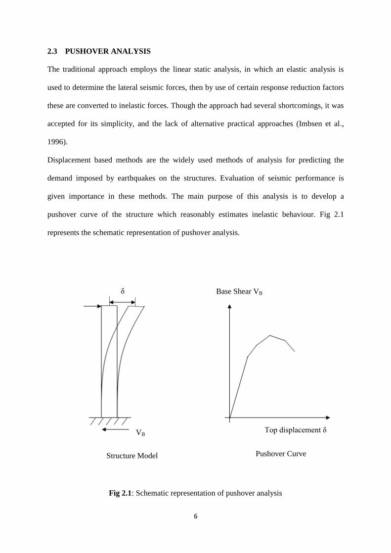
2.3 PUSHOVER ANALYSIS
The traditional approach employs the linear static analysis, in which an elastic analysis is
used to determine the lateral seismic forces, then by use of certain response reduction factors
these are converted to inelastic forces. Though the approach had several shortcomings, it was
accepted for its simplicity, and the lack of alternative practical approaches (Imbsen et al.,
1996).
Displacement based methods are the widely used methods of analysis for predicting the
demand imposed by earthquakes on the structures. Evaluation of seismic performance is
given importance in these methods. The main purpose of this analysis is to develop a
pushover curve of the structure which reasonably estimates inelastic behaviour. Fig 2.1
represents the schematic representation of pushover analysis.
δ
VB
Base Shear VB
Top displacement δ
Structure Model Pushover Curve
Fig 2.1: Schematic representation of pushover analysis
7
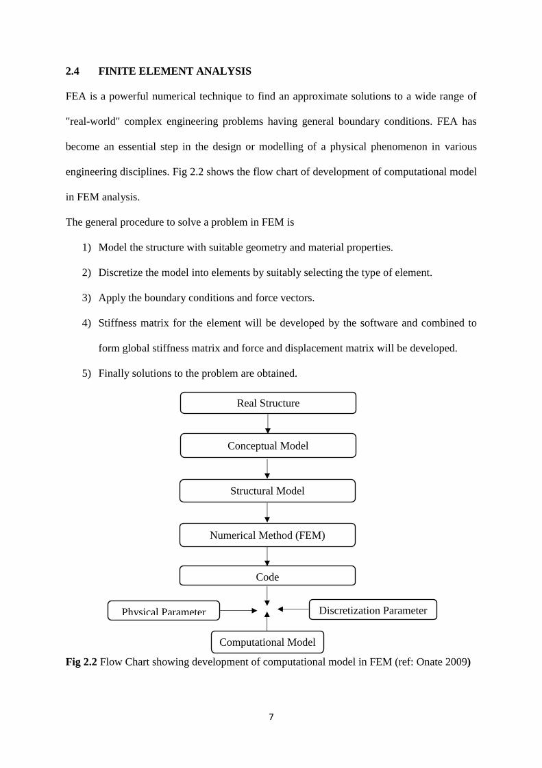
2.4 FINITE ELEMENT ANALYSIS
FEA is a powerful numerical technique to find an approximate solutions to a wide range of
"real-world" complex engineering problems having general boundary conditions. FEA has
become an essential step in the design or modelling of a physical phenomenon in various
engineering disciplines. Fig 2.2 shows the flow chart of development of computational model
in FEM analysis.
The general procedure to solve a problem in FEM is
1) Model the structure with suitable geometry and material properties.
2) Discretize the model into elements by suitably selecting the type of element.
3) Apply the boundary conditions and force vectors.
4) Stiffness matrix for the element will be developed by the software and combined to
form global stiffness matrix and force and displacement matrix will be developed.
5) Finally solutions to the problem are obtained.
Fig 2.2 Flow Chart showing development of computational model in FEM (ref: Onate 2009)
Real Structure
Conceptual Model
Structural Model
Numerical Method (FEM)
Code
Physical Parameter Discretization Parameter
Computational Model

8
2.5 ANALYSIS STEPS INVOLVED IN ABAQUS
In Abaqus modelling and analysis includes following three steps:
1. Pre-processing
2. Simulation
3. Post processing
2.5.1 Pre-processing
In this step model of the physical problem is defined and an abaqus input file (job.inp) in
generated. Basic key points like material properties, boundary condition, load, contact, mesh
are defined here.
2.5.2 Simulation
The simulation is normally run as a background process. In this step already generated
abaqus input file solves the numerical problem defined in the model. For example, output
from a stress analysis problem includes displacement and stress values which stored in binary
files in simulation which are further to be used in post-processing. The output file is
generated as job.odb.
There are three phases in simulation stage
Analysis step
Load increment
Iteration
In first phase, we have to define steps which generally consists of loading option, output
request. Output request describes the values of required parameters like displacement, stress,
strain, reaction force, bending moment etc.

9
Second phase is the increment step, in which first load increment is to be defined by user and
the subsequent increments will be chosen by abaqus automatically. After each load increment
the structure is in equilibrium and corresponding output request values are to be written to the
output database file.
In iteration step, approximate equilibrium solution in each increment is found out. If the
structure is not in equilibrium after iteration, abaqus tries further iteration till closest possible
equilibrium is obtained or the residual force is less than the given tolerance value.
2.5.3 Post processing
Once the simulation is done and the fundamental variables like stress, displacement, reaction
forces are calculated, the results can be evaluated using Visualization module of abaqus. The
visualization module has variety of options to display the results such as animation, colour
contour plots, deformed shape plots and X-Y plots.
2.6 SUMMARY
This Chapter presents the analysis methods used in this study i.e., free vibration analysis,
pushover analysis and finite element analysis. This chapter also presents about the analysis
steps involved in abaqus software.

10
CHAPTER 3
STRUCTURAL MODELLING
3.1 INTRODUCTION
The study in this thesis is based on nonlinear analysis of selected railway bridge piers. This
chapter presents a summary of various parameters defining the computational models. In
structural members, several degradation types takes place like crushing, cracking, damage,
spalling of concrete and yielding of reinforcement. Hence, to accurately model the non-linear
properties of the materials and structural components plays a vital role in non-linear analysis.
In the present study, piers were modelled with inelastic concrete damaged plasticity model
(CDPM) in abaqus.
The response of structure under loading is critical in estimating its efficiency and safety.
Experimental analysis is widely used since it gives real time response but it is time
consuming and costly. The use of finite element packages makes the analyses cost-effective
and we can understand the response of the structure. For the purpose of the modelling it is
important to understand the element types their features and behavior. Therefore it is
necessary to have an idea about the different types of elements used for modelling in finite
element software.
3.2 STRUCTURAL DETAILS
A survey was conducted to obtain the structural details of existing solid mass concrete gravity
bridge pier. As a result details of such bridge piers from seven newly constructed railway
river bridges were obtained. These bridge piers have rectangular section with semi-circular
ends and slanted in both directions. Fig. 3.1 presents the typical elevations along flow and
traffic directions and the typical plan of these bridge piers. The side slope of these bridge

11
piers is found to be equal in both the directions. All of these available piers are rigidly
connected to the pile cap using a number of dowel bars. The pile caps, in all the cases, are
supported by multiple piles. All the railway bridges considered in this study are multi-span
bridges and therefore has multiple piers. The piers of one bridge are identical in shapes and
sizes except for the length. Length of the piers is varying according to the river profile. One
representative pier from each of the seven bridges are considered for analysis. Table 3.1
presents the dimensions of selected seven piers. Mass concrete of M-25 grade was used to
build these piers.
Fig. 3.1: Plan and Elevations of typical Solid Gravity Pier used in this study
H
(a) Pier Section along Flow Direction (b) Pier Section along Traffic Direction
(c) Cross section of the pier

12
Table 3.1: Details of the selected piers
SL.
No.
Height,
H (m)
Base Dimension (m) Top dimensions (m)
Slope (in
both dirn.) Rectangular
Portion
(L×B)
Diameter of
semi-circular
portion, (D)
Rectangular
Portion
(L×B)
Diameter of
Semi-circular
portion, (D)
1 7.500 4×2.50 2.50 4×1.5 1.5 1 in 15
2 10.500 4×2.90 2.90 4×1.5 1.5 1 in 15
3 8.402 4×2.62 2.62 4×1.5 1.5 1 in 15
4 11.250 4×3.75 3.75 4×1.5 1.5 1 in 10
5 16.875 4×4.75 4.75 4×2.5 2.5 1 in 15
6 12.000 4×3.90 3.90 4×1.5 1.5 1 in 10
7 12.375 4×4.15 4.15 4×2.5 2.5 1 in 15
3.3 ELEMENT USED IN ABAQUS
Abaqus element library provides a large variety of elements in modelling different geometries
and structures like beam elements, brick elements, truss elements, membrane elements, shell
elements, quadrilateral elements. Fig 3.2 shows the elements available in the abaqus element
library.
Beam elements:
2 node linear beam element in plane (designation B21 in ABAQUS): This type of elements
has two nodes and each node has three degrees of freedom. Used for plane stress analysis.
2 node linear beam in space (designation B31): It is an element used for simple stress-strain
analysis. It has two nodes and six degrees of freedom at each node at space.
3 node quadratic beam in plane-(designation B22): It is quadratic beam element used for
13
stress analysis. Each element has three nodes. Each nodes carries three degree of freedom.
3 node quadratic beam in space-(designation B32): It is a quadratic element in space which
has three nodes, six degrees of freedom at each node. It is used for stress concentration and
for analysis of beam in space or frame in space.
The solid element library includes isoparametric elements: quadrilaterals in two dimensions
and “bricks” (hexahedra) in three dimensions. These isoparametric elements are generally
preferred for most cases because they are usually the more cost-effective of the elements that
are provided in ABAQUS. They are offered with first- and second-order interpolation.
Standard first-order elements are essentially constant strain elements: the isoparametric forms
can provide more than constant strain response, but the higher order content of the solutions
they give is generally not accurate and, thus, of little value. The second-order elements are
capable of representing all possible linear strain fields. Therefore, it is generally
recommended that the highest-order elements available be used for such cases: in ABAQUS
this means second order elements.
8 node linear brick element reduced integration-(designation C3D8R): It is an 8 node 3D
brick element and on the elemental nodes only the degrees of freedom are calculated and at
other nodes the values are obtained by interpolating with the nodal values. Used for higher
order beam analysis.
20 node quadratic brick element, reduced integration-(designation C3D20R): It is used for
three dimensional model analysis. Degrees of freedom are calculated only element nodes. At
any other point in the element, the values are obtained by interpolating from the nodal values.
Number of element nodes determines the interpolation order. Elements with mid side nodes,
such as the 20-node brick use quadratic interpolation and are often called quadratic elements

14
3 node quadratic 3-D truss element-(designation T3D3): This type of element has three
nodes. It is a basically bar element. For modelling of reinforcement this type of element is
used.
A 2-node linear 3-D truss-(T3D2): This type of element has two nodes. It is used as bar
elements and for reinforcement modelling. It is required for truss member modelling.
8node quadrilateral membrane, reduced integration-(designation M3D8R): Membrane
standard quadratic element. Thin surfaces in space are represented by these type of elements
that offer strength in the plane of the element but have no bending stiffness.
3.4 GEOMETRIC MODELLING
First, in the part module, the base section of the pier is drawn and extruded to the
height, H of the selected pier with slope 1 in N.
In the property module, then material properties i.e., concrete damaged plasticity
model parameters are given and assigned to the section..
In the step module, step is created for the type of analysis. In the present study static
(a) (b) (c)
(d) (e)
Fig 3.2: Finite elements-(a) linear element,; B21,B31 (b) quadratic element; B22,B32
(c) C3D8R (d) C3D20R (e) M3D8R

15
procedure is selected and geometric non-linearity is taken into account by selecting
the Nlgeom-on.
Step General Static Nlgeom
In the load module, boundary conditions are created. Fig 3.3 shows the boundary
conditions applied to the structure. The bottom end of the pier is assumed fixed and
top is displaced to certain displacement. The displacement is applied in incremental
manner.
In the mesh module module, the structure is discretized into finite number of elements. The
structure is discretized using C3D8R element. It is 3D element with 8 nodes with six degrees
of freedom with three translations at each node translations in the nodal x, y, z directions and
rotational along nodal x, y, z directions. At other nodes the displacements, stress, strain
values are calculated by interpolating with the nodal values.
Fig 3.3: Pier model in abaqus

16
3.5 MATERIAL MODELLING
The exact behaviour of the structure cannot be estimated by the elastic material properties
under high intensity loads. Hence non-linear material properties have to be determined for
these type of types. In this study Concrete Damaged Plasticity Model is used for material
modelling.
3.5.1 Concrete Damaged Plasticity Model (CDPM)
The two important failure mechanisms of concrete is assumed to be compression crushing
and tensile cracking. This model represents the complex behaviour of the material by
considering the isotropic damaged elasticity with isotropic tensile and compressive plasticity.
Lubliner et al. 1989 first proposed this model and later was consolidated by Lee and Fenves
1998. Concrete Damaged Plasticity Model was put into implementation in FEM software
(ABAQUS). The potential plastic flow is assumed in the model G and it is the Drunker-
Prager hyperbolic function:
𝐺 = √(∈ 𝜎𝑡𝑜 tan 𝜓)2 + �̅�2 − �̅� tan 𝜓
𝜎𝑡𝑜 is the uniaxial tensile stress at failure, 𝑝 ̅ is the hydrostatic pressure stress, �̅� is the Mises
equivalent effective stress, 𝜓 is the dilatency angle measured in the p-q plane at high
confining pressure and 𝜖 is an eccentricity of the plastic potential surface. This model makes
use of a yield state centred on loading function F proposed by Lubliner et al. 1989 with the
changes made by Lee and Fenves 1998 to account for evolution of strength under tension and
compression in the form:
𝐹 =1
1 − 𝛼(�̅� − 3𝛼�̅� + 𝛽( 𝜀̃𝑝𝑙⟨𝜎𝑚𝑎𝑥⟩ − 𝛾⟨−𝜎𝑚𝑎𝑥⟩) − 𝜎𝑐𝜀̃𝑝𝑙 = 0
𝛼 =(𝜎𝑏𝑜 𝜎𝑐𝑜⁄ ) − 1
2(𝜎𝑏𝑜 𝜎𝑐𝑜 − 1)⁄ ; 0 < 𝛼 < 0.5
𝛽 =𝜎�̅�(𝜀�̃�
𝑝𝑙)
𝜎𝑡(𝜀�̃�𝑝𝑙)
(1 − 𝛼) − (1 + 𝛼)

17
𝛾 =3(1 − 𝐾𝑐)
2𝐾𝑐 − 1
Factor 𝛼 depends on the ratio of the biaxial and uniaxial compressive strengths (𝜎𝑏𝑜 𝜎𝑐𝑜)⁄ , 𝐾𝑐
is the ratio of magnitude of the deviatory stress in uniaxial tension to the uniaxial
compression and it should satisfy the limit of 0.5< 𝐾𝑐 < 1.0. Thus it clearly understood that
the concrete behaviour depends on four constitutive parameter (𝐾𝑐 ,𝜓, (𝜎𝑏𝑜 𝜎𝑐𝑜)⁄ , 𝜖). The
other parameters include the stress-strain behaviour of concrete in compression and tension.
Concrete exhibits softening behaviour and stiffness degradation that leads to convergence
difficulties, hence to allow stresses to be outside the yield surface a viscosity factor 𝜇 has
been added to the CPDM in abaqus.
The value of Kc is determined by Mohr Coulomb yield surface function and its value controls
the shape of the yield surface if Kc = 1 the yield surface is a circle and Kc = 0.5 the yield
surface is a triangle. (fig 3.4)
Fig 3.4: Yield Surface for Kc = 1 and Kc = 0.5
Dilatancy angle (𝜓): It is the phenomenon of change of the inelastic volume to plastic
deviation in a frictional material during shearing.
Kc=1
Kc=0.5

18
(b) No dilation (a) With dilation
Fig 3.5: Dilatency angle
In the first case (fig 3.5 (a)) the square has undergone distortion and no volumetric strain i.e.,
no dilation. In the second case fig 3.5 (b)) the square has undergone distortion with
volumetric strain, the amount by which this distortion takes place is called dilation angle.
(𝜓=380 (ref. Jankowiak et al., (2005).)
Table 3.2: CPDM parameters used in this study
𝐾𝐶 Dilatency
angle (𝜓) 𝜎𝑏𝑜 𝜎𝑐𝑜⁄ 𝜖 𝜇
0.67 380 1.16 0.1 0.0001
3.5.2 Uniaxial Compression behaviour of concrete:
The stress-strain compression concrete model used in this study was developed by Hsu-Hsu
(1994). Fig 3.6 shows the compression stress strain curve developed by Hsu Hsu (1994). This
stress strain behaviour is modelled in three stages. The first two stages defines the ascending
branch of the curve and the third one descending portion of the curve.
.
𝜓

19
Fig 3.6: Uniaxial Compressive Stress Strain Curve (Hsu Hsu model)
1) In the ascending portion of the branch upto 50% of the ultimate compressive strength
(𝜎𝑐𝑢) , a linear stress strain relationship which obeys Hooke’s law is assumed.
𝜎𝑐 = 𝐸𝑜𝜀𝑐
2) From 0.5𝜎𝑐𝑢 to the ultimate stress 𝜎𝑐𝑢 a non-linear nature of concrete is modelled
using the following equations.
3) In the descending portion upto 0.3𝜎𝑐𝑢 the stress strain curve is modelled.
The Hsu Hsu model (1994) is used to calculate the compression stress strain values only after
the yield i.e., 0.5 𝜎𝑐𝑢 in the ascending branch to the 0.3𝜎𝑐𝑢 in the descending branch.
𝜎𝑐 = [𝛽(
𝜀𝑐𝜀𝑜
⁄ )
𝛽 − 1 + (𝜀𝑐
𝜀𝑜⁄ )𝛽
]𝜎𝑐𝑢
The parameter 𝛽 defines the shape of the stress strain curve after yielding of concrete at
0.5𝜎𝑐𝑢
0.3
𝜎𝑐𝑢
0.5
𝜎𝑐
𝑢
𝜎𝑐𝑢
𝜀𝑜 𝜀𝑑 Strain, 𝜀𝑐
Str
ess,
𝜎𝑐

20
𝛽 =1
1 − [𝜎𝑐𝑢
(𝜀0𝐸𝑜)⁄ ]
The modulus of elasticity is given by
𝐸𝑜 = 1.2431𝑥102 + 3.28312𝑥103
Strain 𝜀𝑜 at the ultimate compressive stress 𝜎𝑐𝑢 is given by
𝜀𝑜 = 8.9𝑥10−5𝜎𝑐𝑢 + 2.114𝑥10−3
The units in the above equations are in 𝑘𝑖𝑝 𝑖𝑛2⁄
The inelastic strains are to be entered in the CDPM corresponding to the stresses and it is
given by
𝜀�̃�𝑖𝑛 = 𝜀𝑐 − 𝜀𝑜𝑐
𝑒𝑙
Where, 𝜀𝑜𝑐𝑒𝑙 =
𝜎𝑐
𝐸𝑐 is the elastic strain corresponding to the un-yielded material.
𝜀𝑐 is the total strain corresponding to the particular stress value.
3.5.3 Uniaxial Tension of Concrete:
The complete tensile stress-strain behaviour of concrete which accounts for strain-softening,
tension stiffening is necessary for the simulation in abaqus. Hence we have to input the
values of young’s modulus 𝐸0, stress 𝜎𝑡, cracking strain 𝜀𝑐𝑟 and the damage parameter values
𝑑𝑡corresponding to the grade of concrete used. The cracking strain can be calculated from the
total stain using the following equation
𝜀�̃�𝑐𝑘 = 𝜀𝑡 − 𝜀𝑜𝑡
𝑒𝑙
𝜀𝑡 is the total stain and 𝜀𝑜𝑡𝑒𝑙 =
𝜎𝑡
𝐸0 is the elastic stain for the un-yielded material.
21
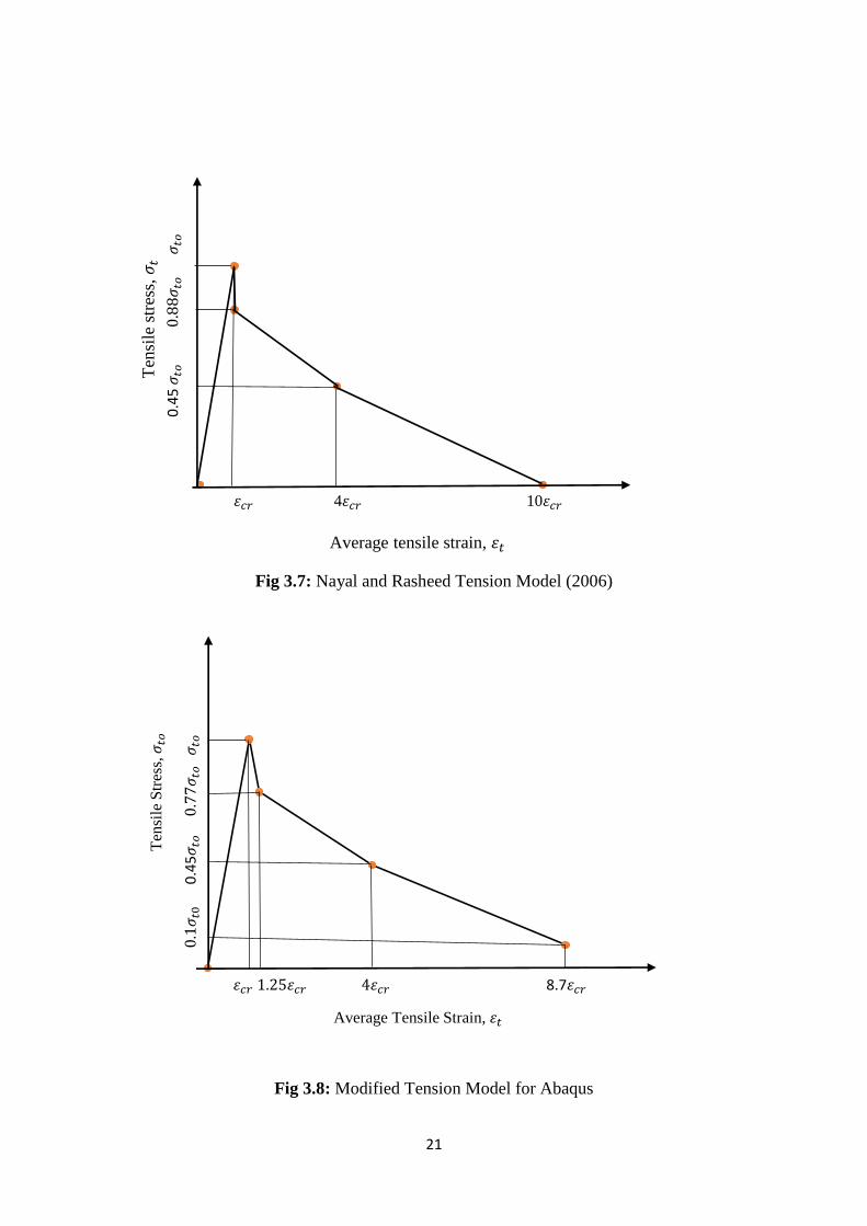
Fig 3.7: Nayal and Rasheed Tension Model (2006)
Fig 3.8: Modified Tension Model for Abaqus
0.1
𝜎𝑡0
0.4
5𝜎
𝑡𝑜
0.7
7𝜎
𝑡𝑜
𝜎𝑡𝑜
𝜀𝑐𝑟 1.25𝜀𝑐𝑟 4𝜀𝑐𝑟 8.7𝜀𝑐𝑟
Average Tensile Strain, 𝜀𝑡
Ten
sile
Str
ess,
𝜎𝑡𝑜
𝜀𝑐𝑟 4𝜀𝑐𝑟 10𝜀𝑐𝑟
0
.45
𝜎𝑡𝑜
0
.88
𝜎𝑡𝑜
𝜎𝑡𝑜
Average tensile strain, 𝜀𝑡
Ten
sile
str
ess,
𝜎𝑡

22
The tensile stress strain model of concrete used in this study was developed by Nayal and
Rasheed (2006) (fig 3.7). This model resemblance the tension stiffening model required for
the CDPM in abaqus. The descending portion of the tensile stress strain is based on the
cracking phenomena developed by Gilbert and Warner (1978). The abrupt drop at maximum
tensile strain 𝜀𝑐𝑟 from ultimate tensile stress 𝜎𝑡𝑜 to 0.8𝜎𝑡𝑜 as observed by Nayal and Rasheed
(2006) is sloped from (𝜀𝑐𝑟 , 𝜎𝑡𝑜) to (1.25𝜀𝑐𝑟, 0.77𝜎𝑡𝑜) to eliminate run time errors during
analysis in abaqus. Fig 3.6 shows the modified tension stiffening model for abaqus (fig 3.8).
Apart from that exactly the same stress strain curve developed by Nayal and Rasheed (2006)
is adopted.
3.5.4 Damage Parameter
The plastic strain 𝜀𝑐𝑝𝑙
is proportional to the inelastic strain 𝜀�̃�𝑖𝑛 using a constant 𝑏𝑐(0< 𝑏𝑐 < 1)
and is related to the compressive damage by the following equation model behaves simply as
plastic model if these parameters are not defined. The damage variables are considered as
non-decreasing values. At any increment during the analysis, the new value of each damage
variable is obtained as the maximum between the value at the end of the previous increment
and the value corresponding to the current state
𝑑𝑐 = 1 −(𝜎𝑐 𝐸𝑐)⁄
𝜀𝑝𝑙(1 𝑏𝑐 − 1) + (𝜎𝑐 𝐸𝑐)⁄⁄
Similarly in the tension zone
𝑑𝑡 = 1 −(𝜎𝑡 𝐸𝑐)⁄
𝜀𝑝𝑙(1 𝑏𝑐 − 1) + (𝜎𝑡 𝐸𝑐)⁄⁄
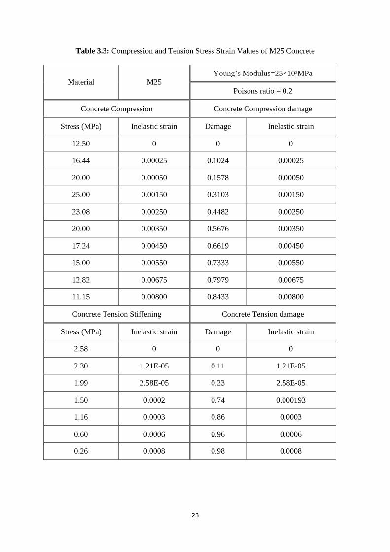
In the present all the selected piers are modelled using M25 grade concrete using Hsu-Hsu
Concrete compression model and Nayal and Rasheed (2006) tension stiffening model. Table
3.3 shows the uniaxial compression and tension stress strain values used to model the piers in
the present study.
23
Table 3.3: Compression and Tension Stress Strain Values of M25 Concrete
Material M25 Young’s Modulus=25×10³MPa
Poisons ratio = 0.2
Concrete Compression Concrete Compression damage
Stress (MPa) Inelastic strain Damage Inelastic strain
12.50 0 0 0
16.44 0.00025 0.1024 0.00025
20.00 0.00050 0.1578 0.00050
25.00 0.00150 0.3103 0.00150
23.08 0.00250 0.4482 0.00250
20.00 0.00350 0.5676 0.00350
17.24 0.00450 0.6619 0.00450
15.00 0.00550 0.7333 0.00550
12.82 0.00675 0.7979 0.00675
11.15 0.00800 0.8433 0.00800
Concrete Tension Stiffening Concrete Tension damage
Stress (MPa) Inelastic strain Damage Inelastic strain
2.58 0 0 0
2.30 1.21E-05 0.11 1.21E-05
1.99 2.58E-05 0.23 2.58E-05
1.50 0.0002 0.74 0.000193
1.16 0.0003 0.86 0.0003
0.60 0.0006 0.96 0.0006
0.26 0.0008 0.98 0.0008

24
3.6 SUMMARY
This chapter presents details of selected railway bridge piers and describes about the
Concrete Damaged Plasticity model which is used for nonlinear material modelling. It
describes about the Abaqus simulation process and different types of elements available in
the element library and finally about the modelling of the piers selected for the present study.

25
CHAPTER 4
RESULTS AND DISCUSSIONS
4.1 INTRODUCTION
The selected railway bridge pier models are analysed using modal analysis and non-linear
static (pushover analysis). This chapter presents elastic modal properties of the selected piers,
pushover analysis results and discussions. Then a lateral pushover analysis in transverse
direction was performed in a displacement control manner.
4.2 RESULTS FROM MODAL ANALYSIS
Modal properties of the selected railway bridge piers were obtained from the linear dynamic
modal analysis. Table 4.1 shows the details of the important modes of the bridge in X direction.
The table shows that the percentage of mass participation in the first mode is zero and the
cumulative mass participating percentage in the first six modes is between 65%-85%. Hence, the
higher mode participation in the response of railway bridge pier is significant unlike in regular
buildings where only fundamental mode contribution is vital. Table 4.2 shows the cumulative
mass participation in X and Y directions for first six modes.
Table 4.1: Elastic Modal Properties for Bridge pier # 6
Mode No. Frequency (Hz) Time period
(s)
Cumulative Mass
Participation (UX)
Cumulative Mass
Participation (UY)
1 15.66 0.0638 0 0.44
2 28.77 0.0347 0.48 0.44
3 46.78 0.0214 0.48 0.44
4 56.56 0.0177 0.48 0.67
5 84.80 0.0118 0.48 0.67
6 85.05 0.0118 0.73 0.67

26
Table 4.2: Cumulative Mass Participation of selected piers in first six mode
Pier No. UX UY
1. 0.73 0.66
2. 0.75 0.71
3. 0.61 0.55
4. 0.80 0.75
5. 0.78 0.71
6. 0.79 0.74
7. 0.78 0.75
Fig. 4.1 shows the mode shapes of pier# 6 for first six modes. From this figure (also from the
Table 4.1) it can be seen that first two fundamental period reflects the translatory motion of the
pier in two orthogonal horizontal directions (X- and Y- directions) with significant mass
participation although the participating mass ratio in these two modes are below 50% in this
case. It can be observed from this figure that torsional mode (Mode# 3) and the rocking mode
(Mode# 5) do not contribute anything in the mass participation. Two bending modes (Mode# 4
and Mode# 6) contributes significant amount of mass participation.
(a) Mode shape # 1

27
(b) Mode Shape # 2
(c) Mode Shape # 3
(d) Mode Shape # 4

28
(e) Mode Shape # 5
(f) Mode Shape # 6
Fig 4.1: First six Mode shapes of pier # 6
4.3 RESULTS FROM PUSHOVER ANALYSIS
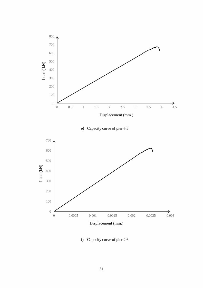
Pushover analysis is carried out on the selected railway bridge piers using displacement
controlled method and the capacity curves of the piers are plotted. Fig. 4.2 shows the resulting
capacity curve of all the seven bridge piers analysed in this study.
This figures show that the brittle mode of failure of all the bridge piers at ultimate load. This is
due to poor energy dissipation capacity of the mass concrete used for building this structures.
Table 4.3 presents the summary of the pushover analysis results obtained in the presents study.

29
a) Capacity Curve for pier # 1
b) Capacity curve of pier # 2
0
100
200
300
400
500
0 0.2 0.4 0.6 0.8 1 1.2 1.4
Displacement ( mm.)
Load
(kN
)
0
100
200
300
400
500
0 0.5 1 1.5 2 2.5
Load
(kN
)
Displacement (mm.)

30
c) Capacity curve of pier # 3
d) Capacity curve for pier # 4
0
100
200
300
400
500
0 0.2 0.4 0.6 0.8 1 1.2 1.4 1.6
Load
(kN
)
Displacement (mm.)
0
100
200
300
400
500
600
700
0 0.5 1 1.5 2 2.5
Displacement (mm.)
Load
(kN
)
31
e) Capacity curve of pier # 5
f) Capacity curve of pier # 6
0
100
200
300
400
500
600
700
800
0 0.5 1 1.5 2 2.5 3 3.5 4 4.5
Load
( k
N)
Displacement (mm.)
0
100
200
300
400
500
600
700
0 0.0005 0.001 0.0015 0.002 0.0025 0.003
Displacement (mm.)
Load
(kN
)

32
g) Capacity curve for pier # 7
Fig 4.2: Capacity curves of the seven selected piers
Table 4.3: Summary of the pushover analysis results
Pier# Weight,
W (kN)
Base Area
(m2)
Height, h
(m)
Top
Disp.,
(mm)
Base
Shear, VB
(kN) W
VB
Drift
Ratio,h
(×10-3
)
1 2040 14.91 7.500 1.23 462 0.226 0.164
2 3272 18.21 10.500 1.97 426 0.131 0.188
3 2383 15.87 8.402 1.42 448 0.188 0.169
4 4564 26.04 11.250 2.27 615 0.135 0.202
5 10454 36.72 16.875 3.93 675 0.065 0.233
6 5085 27.55 12.000 2.50 624 0.123 0.208
7 6687 30.13 12.375 2.40 712 0.107 0.194
0
100
200
300
400
500
600
700
800
0 0.5 1 1.5 2 2.5 3
Displacement ( mm.)
Lo
ad (
kN
)

33
Table 4.3 shows that the displacement limit state of collapse occurs at a base shear range of 6.5-
22.6% of the total weight and a drift ratio of 0.0164% to 0.0233%. This table shows that the
base shear capacity of the bridge pier (VB/W) is inversely proportional to the pier height.
Fig. 4.3 presents a scatter of (VB/W) versus pier height.
Fig. 4.3: (VB/W) versus pier height scatter
y = -0.0165x + 0.3255 R² = 0.9022
0
0.05
0.1
0.15
0.2
0.25
5 10 15 20
VB/W
Height of the pier

34
CHAPTER 5
SUMMARY AND CONCLUSIONS
5.1 SUMMARY
Most of the sub-structures of new railway river bridges in the state of Odisha are built with
solid mass concrete gravity piers and abutments. These piers do not have steel reinforcement
to bear the load as it does not subject to any tensile stress under regular type of loading.
Safety of these piers is of major concern during high magnitude earthquake.
This study aims to assess the vulnerability of the solid gravity bridge piers which forms the
important component of railway bridges as the load transfer between substructure and
superstructure takes through them. In the present study seven existing piers from the state of
Odisha are evaluated using free vibration analysis and nonlinear static (pushover) analysis.
5.2 CONCLUSIONS
The significant conclusion drawn from the present study is as follows:
i) Free-vibration analysis of the bridge pier shows that the first two fundamental modes
reflect the translatory motion of the pier in two orthogonal horizontal directions (X-
and Y- directions) with mass participation below 50% for both of the two modes.
ii) The participating mass ratio for torsional mode (Mode# 3) and the rocking mode
(Mode# 5) found to be zero.
iii) The cumulative mass participation for first six mode is found to be less than 80% for
all the selected bridge pier. This indicates the significant contribution of higher
modes.
iv) The pushover analysis indicates the brittle mode of failure of all the bridge piers at
ultimate load. This is due to poor energy dissipation capacity of the mass concrete
used for building these structures.
35
REFERENCES
1. Abaqus Analysis user manual – Abaqus Version 6.12.
2. Birtel, V., Mark, P., (2006), “Parameterised Finite Element Modelling of RC Beam
Shear Failure” ABAQUS Users’ Conference, 95-104.
3. Chang Su Shim, Chul-Hun Chung, Hyun Ho Kim (2008), “Experimental
evaluation of seismic performance of precast segmental bridge piers with a circular
solid section”, Engineering Structures, 30, 3782-3792.
4. Cheng, C. (2007), “Energy dissipation in rocking bridge piers under free vibration
tests”, Earthquake Engineering Structural Dynamics, 36, 503-518.
5. Cho, C., Han, S., Kwon, M. and Lim, C. (2012), “Seismic Performance Evaluation
of Reinforced Concrete Columns by Applying Steel Fiber-Reinforced Mortar at
Plastic Hinge Region”, Journal of the Korea Concrete Institute, 24, 241-248.
6. Dassault Systèmes Simulia Corp. Abaqus v. 6.12 [Software].
7. Do Hyung Lee, Eunsoo Choi, Goangseup Zi (2005), “Evaluation of earthquake
deformation and performance for RC bridge piers”, Engineering Structures, 27,
1451-1464.
8. Hsu, L.S., & Hsu, C.-T.T. (1994), “Complete stress-strain behaviour of high-
strength concrete under compression”, Magazine of Concrete Research, 46, 301-
312.
9. Huili Wang, Wang, H., Qin, S.F., Xu, W.J., (2011), “Seismic analysis of
Prestressed Bridge Pier Based on Fiber Section”, International Conference on
Green Buildings and Sustainable Cities, 21, 354–362.
10. Kim, T.-H., Kim, B.S., Chung, Y.-S., Shin, H.M., (2006), “Seismic performance
assessment of reinforced concrete bridge piers with lap splices” Engineering
Structures, Vol. 28, pp. 935–945.

36
11. Lee, J., Fenves, GL., (1998), “Plastic-Damage Model for Cyclic Loading of
Concrete Structures”, Engineering Mechanics, 124, 892–900.
12. Lubliner, J., Oliver, J., Oller, S., Oñate, E., (1989), “A plastic-damage model for
concrete, International Journal of Solids and Structures”, 25, 299–326.
13. Memari, A.M., Harris, H.G., Hamid, A.A., and Scanlon, A., (2011), “Seismic
Evaluation of Reinforced Concrete Piers in Low to Moderate Seismic Regions”,
Electronic Journal of Structural Engineering, 11, 57-68.
14. Nayal, R., Rasheed, H.A. (2006), “Tension Stiffening Model for Concrete Beams
Reinforced with Steel and FRP Bars”, Journal of Materials in Civil Engineering,
18, 831-841.
15. Rui Faria, Nelson Vila Pouca and Raimundo Delgado (2000) “Seismic behaviour
of r/c bridge piers: numerical simulation and experimental validation”, The 12th
World Conference on Earthquake Engineering, No.0673
16. Spyrak, C. C. (1992), “Seismic behavior of bridge piers including soil-structure
interaction” Computers & Structures, 43, 373-384.
17. Wahalathantri, B.L., Thambiratnam, D.P., Chan, T.H.T., & Fawzia, S. (2011), “A
material model for flexural crack simulation in reinforced concrete elements using
abaqus”, eddBE2011 proceedings, 260-264
18. Wang, D.S., Ai, Q.H., Li, H.N., Si, J., and Sun, Z.G. (2008), “Displacement based
seismic design of RC bridge piers: Method and experimental evaluation”, The 14th
World Conference on Earthquake Engineering Beijing, China.


