Download - Lecture 04 Feature Extraction 2 - UZH

Lecture 05 Feature Extraction 1
Prof. Dr. Davide Scaramuzza

REMINDER: Lab Exercise 2 - Today
• At 14:15 in room 2.A.01
• Harris corner detector
• Download: http://rpg.ifi.uzh.ch/docs/teaching/ex02_harris.zip

Outline
• Filters for feature extraction
• Point-feature extraction: today and next lecture
• Line extraction algorithms: next lecture
Filters for features
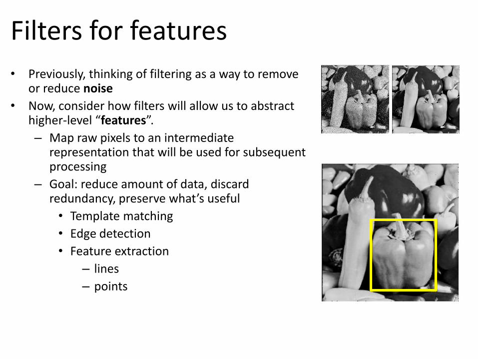
• Previously, thinking of filtering as a way to remove or reduce noise
• Now, consider how filters will allow us to abstract higher-level “features”.
– Map raw pixels to an intermediate representation that will be used for subsequent processing
– Goal: reduce amount of data, discard redundancy, preserve what’s useful
• Template matching
• Edge detection
• Feature extraction
– lines
– points

Template
Detected template
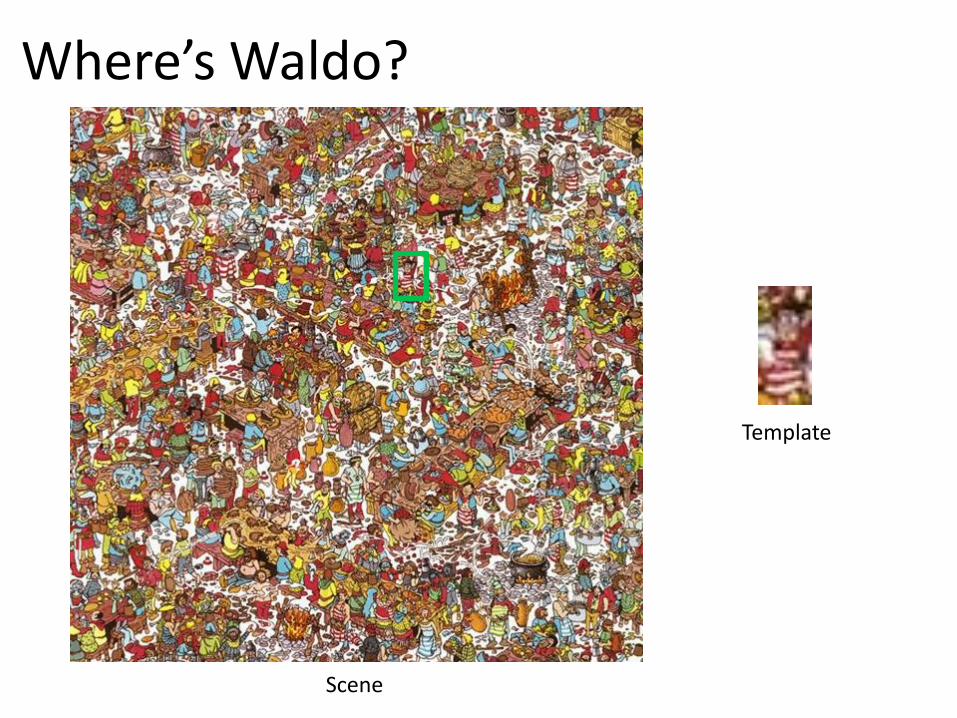
• Find locations in an image that are similar to a template
• If we look at filters as templates, we can use correlation to detect these locations
Filters as Templates

Detected template
• Find locations in an image that are similar to a template
• If we look at filters as templates, we can use correlation to detect these locations
Correlation map
Template matching
Scene
Template
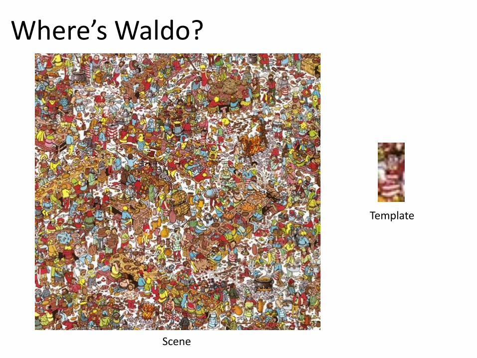
Where’s Waldo?
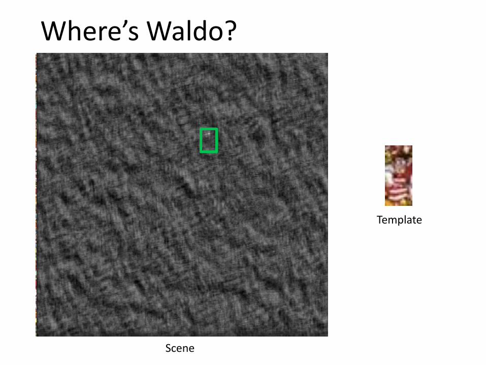
Where’s Waldo?
Scene
Template
Scene
Template
Where’s Waldo?
Scene
Template
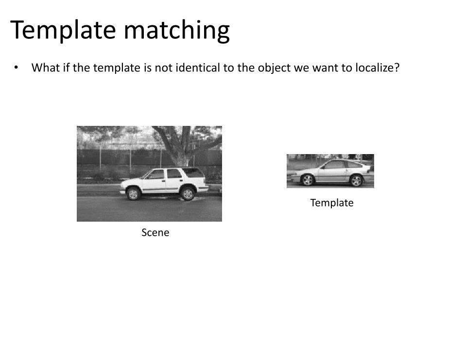
• What if the template is not identical to the object we want to localize?
Template matching

Detected template
Template matching • What if the template is not identical to the object we want to localize? • Match can be meaningful if scale, orientation, illumination, and general
appearance are right
Template
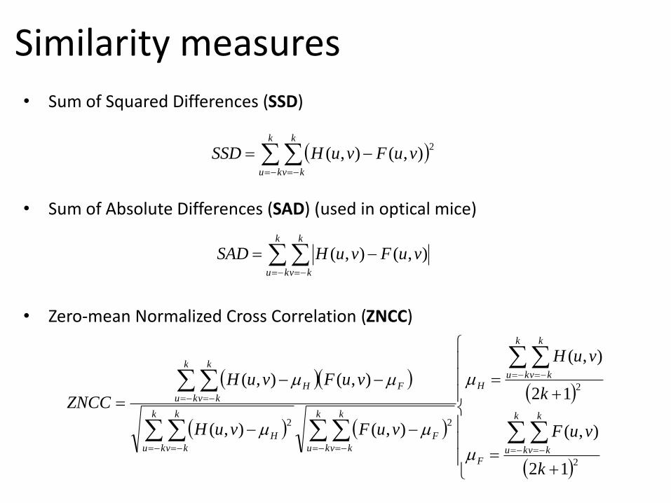
Similarity measures
• Sum of Squared Differences (SSD)
• Sum of Absolute Differences (SAD) (used in optical mice)
• Zero-mean Normalized Cross Correlation (ZNCC)
k
ku
k
kv
F
k
ku
k
kv
H
k
ku
k
kv
FH
vuFvuH
vuFvuH
ZNCC22
),(),(
),(),(
2
2
12
),(
12
),(
k
vuF
k
vuH
k
ku
k
kvF
k
ku
k
kvH
k
ku
k
kv
vuFvuHSSD2
),(),(
k
ku
k
kv
vuFvuHSAD ),(),(
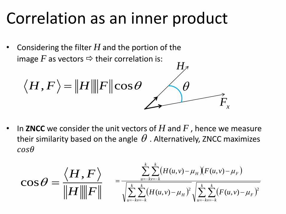
Correlation as an inner product
• Considering the filter H and the portion of the
image F as vectors their correlation is:
• In ZNCC we consider the unit vectors of H and F , hence we measure their similarity based on the angle . Alternatively, ZNCC maximizes 𝑐𝑜𝑠𝜃
cos, FHFH
H
xF
FH
FH ,cos
k
ku
k
kv
F
k
ku
k
kv
H
k
ku
k
kv
FH
vuFvuH
vuFvuH
22),(),(
),(),(
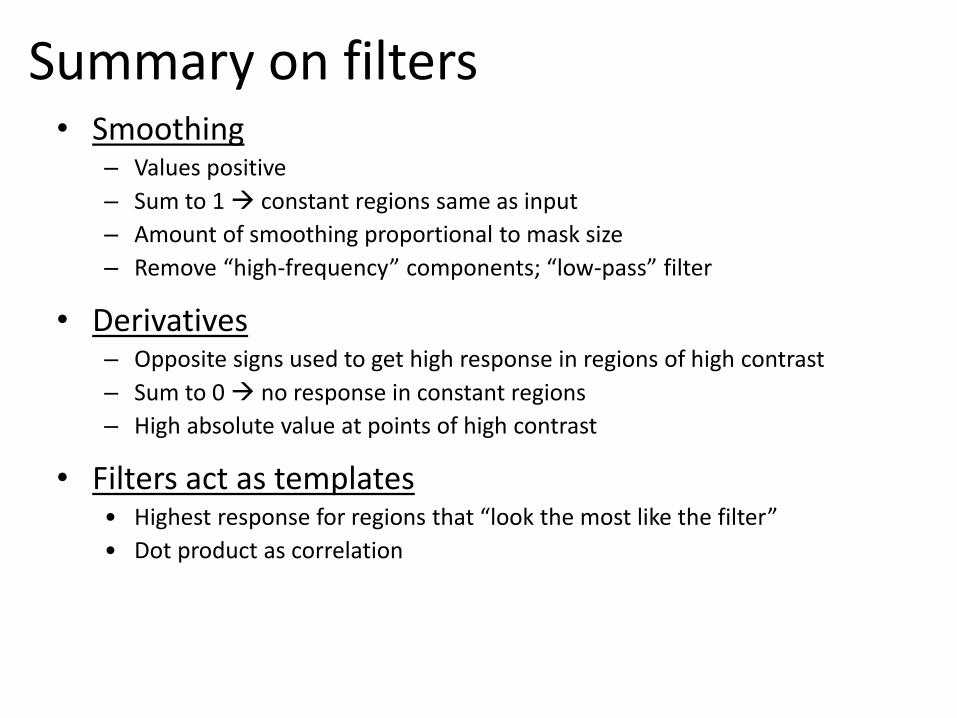
Summary on filters • Smoothing
– Values positive
– Sum to 1 constant regions same as input
– Amount of smoothing proportional to mask size
– Remove “high-frequency” components; “low-pass” filter
• Derivatives – Opposite signs used to get high response in regions of high contrast
– Sum to 0 no response in constant regions
– High absolute value at points of high contrast
• Filters act as templates • Highest response for regions that “look the most like the filter”
• Dot product as correlation
Outline
• Filters for feature extraction
• Point-feature extraction: today and next lecture
• Line extraction algorithms: next lecture
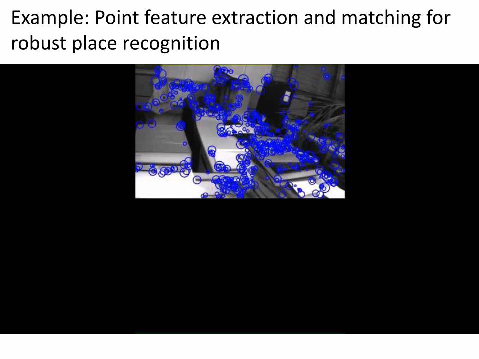
Example: Point feature extraction and matching for robust place recognition
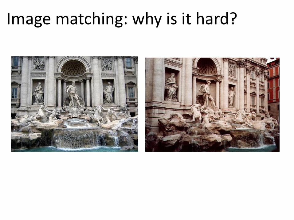
Image matching: why is it hard?

NASA Mars Rover images
Image matching: why is it hard?

NASA Mars Rover images with SIFT feature matches
Image matching: why is it hard? Answer below
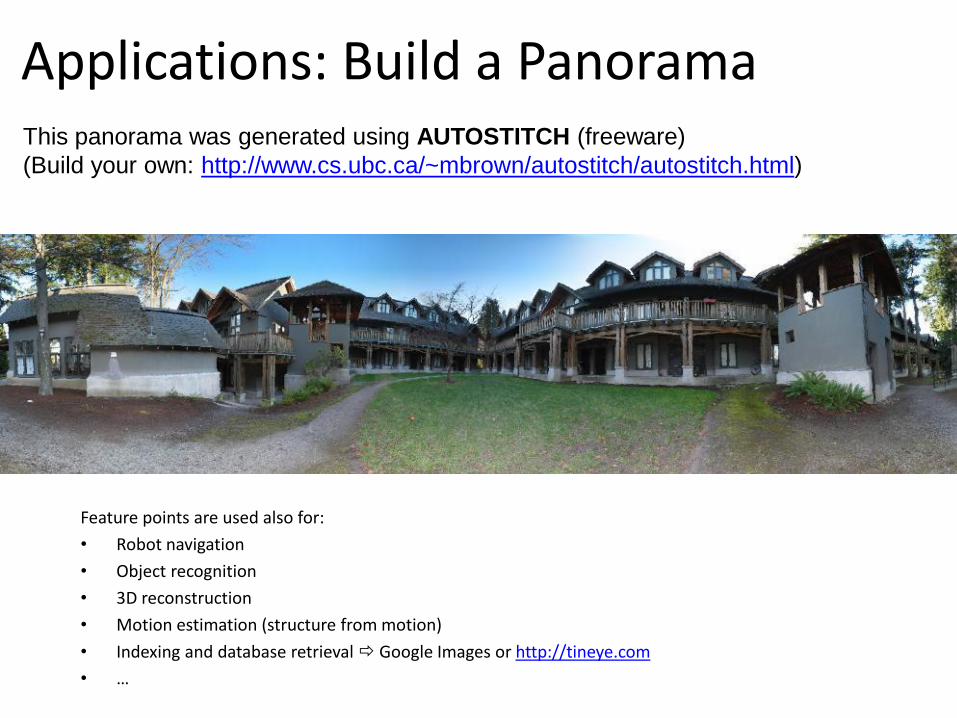
Applications: Build a Panorama This panorama was generated using AUTOSTITCH (freeware)
(Build your own: http://www.cs.ubc.ca/~mbrown/autostitch/autostitch.html)
Feature points are used also for:
• Robot navigation
• Object recognition
• 3D reconstruction
• Motion estimation (structure from motion)
• Indexing and database retrieval Google Images or http://tineye.com
• …

• We need to match (align) images
• How would you do it by eye?
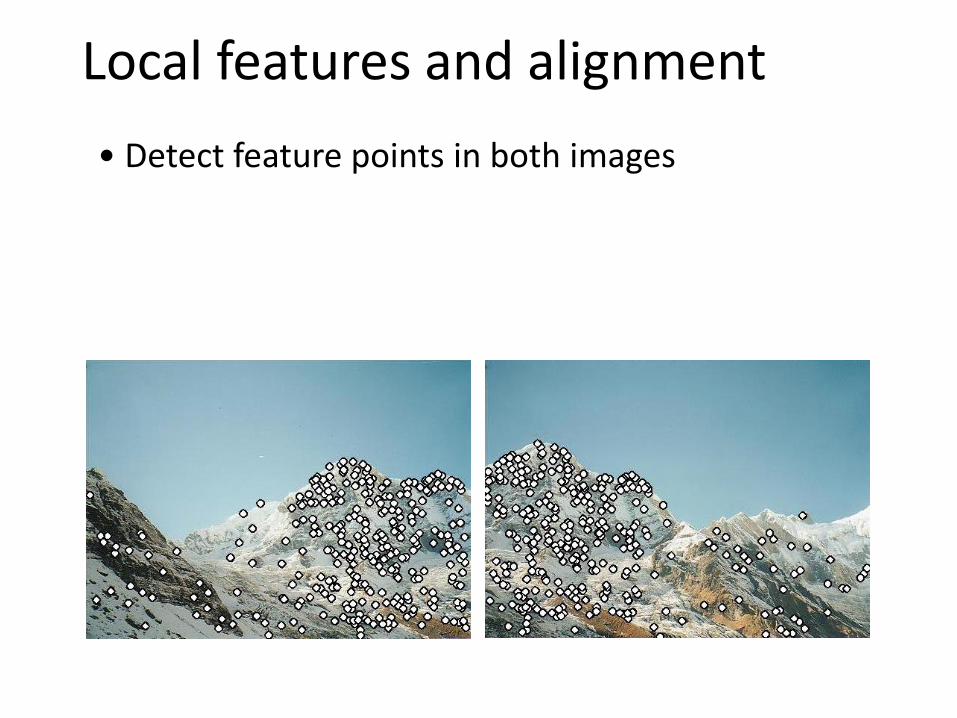
Local features and alignment
Local features and alignment
• Detect feature points in both images
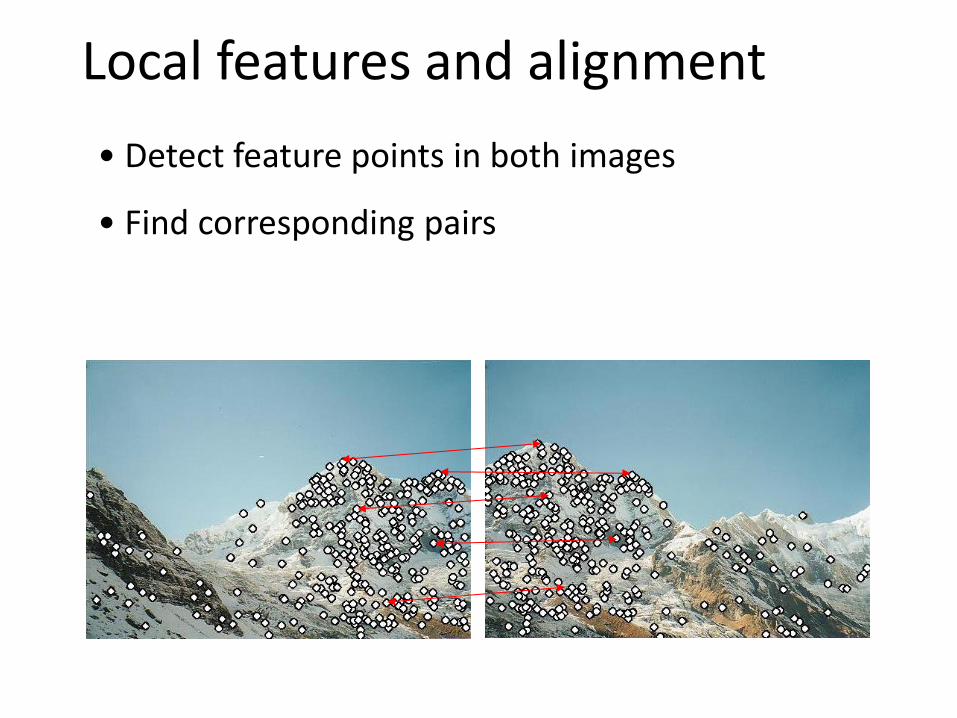
Local features and alignment
• Detect feature points in both images
• Find corresponding pairs

Local features and alignment
• Detect feature points in both images
• Find corresponding pairs
• Use these pairs to align images
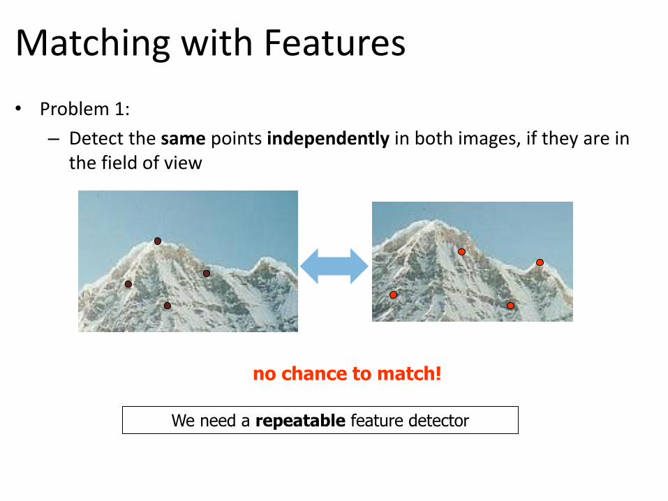
Matching with Features
• Problem 1:
– Detect the same points independently in both images, if they are in the field of view
We need a repeatable feature detector
no chance to match!

Matching with Features
• Problem 2:
– For each point, identify its correct correspondence in the other image(s)
We need a reliable and distinctive feature descriptor
?

Geometric changes
• Rotation
• Scale (i.e., zoom)
• View point (i.e, perspective changes)
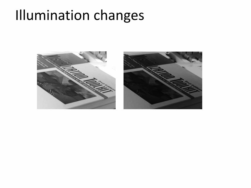
Illumination changes
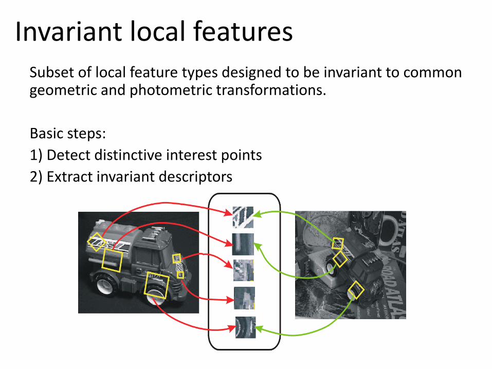
Invariant local features Subset of local feature types designed to be invariant to common geometric and photometric transformations.
Basic steps:
1) Detect distinctive interest points
2) Extract invariant descriptors

Main questions
• What features are salient ? (i.e., that can be re-detected from other views)
• How to describe a local region?
• How to establish correspondences, i.e., compute matches?
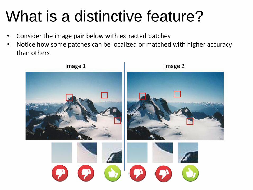
What is a distinctive feature? • Consider the image pair below with extracted patches • Notice how some patches can be localized or matched with higher accuracy
than others
Image 1 Image 2
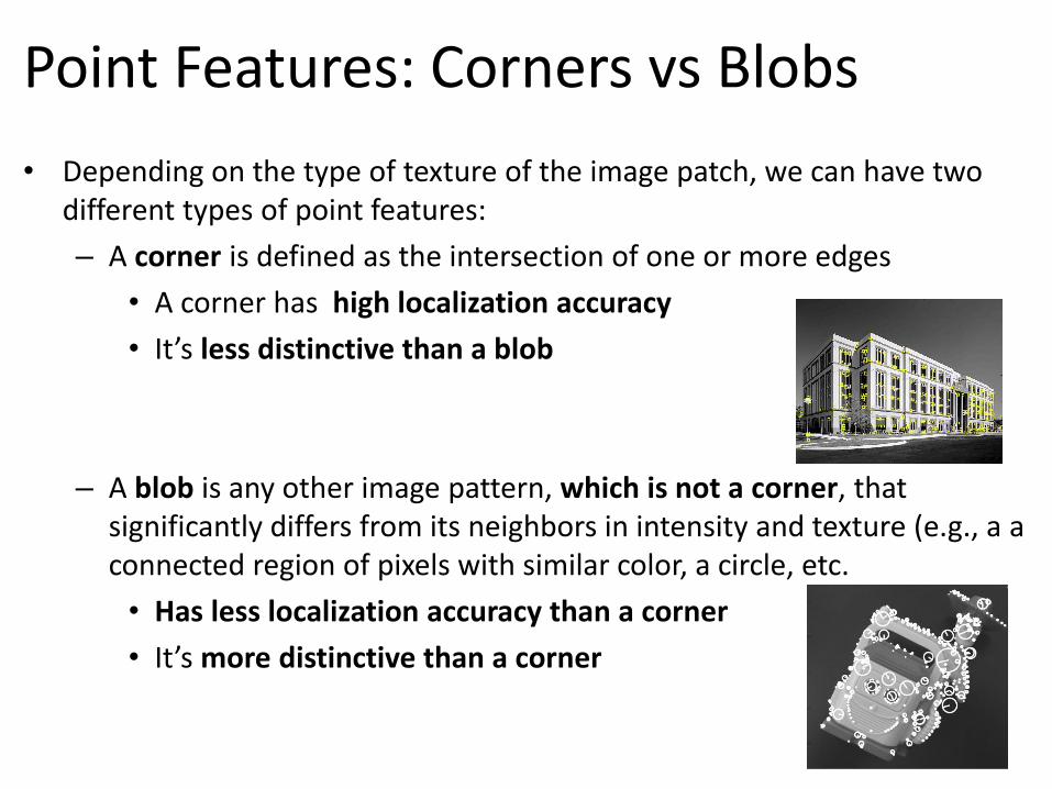
Point Features: Corners vs Blobs
• Depending on the type of texture of the image patch, we can have two different types of point features:
– A corner is defined as the intersection of one or more edges
• A corner has high localization accuracy
• It’s less distinctive than a blob
– A blob is any other image pattern, which is not a corner, that significantly differs from its neighbors in intensity and texture (e.g., a a connected region of pixels with similar color, a circle, etc.
• Has less localization accuracy than a corner
• It’s more distinctive than a corner
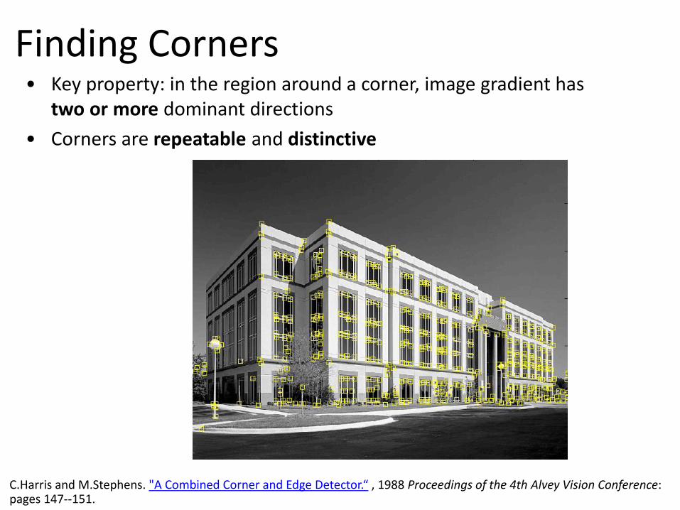
Finding Corners • Key property: in the region around a corner, image gradient has
two or more dominant directions
• Corners are repeatable and distinctive
C.Harris and M.Stephens. "A Combined Corner and Edge Detector.“ , 1988 Proceedings of the 4th Alvey Vision Conference: pages 147--151.

Identifying Corners • How do we identify corners?
• We can easily recognize the point by looking through a small window
• Shifting a window in any direction should give a large change in intensity (e.g., in SSD) in at least 2 directions
“flat” region:
no intensity change
(i.e., SSD ≈ 0 in all directions)
“corner”:
significant change in at least 2
directions
(i.e., SSD ≫ 0 in all directions)
“edge”:
no change along the edge
direction
(i.e., SSD ≈ 0 along edge but
≫ 0 in other directions)

• Consider two image patches of size P. One centered at and one centered at
• The Sum of Squared Differences between them is:
• Let and . Approximating with a 1st order Taylor expansion:
• This produces the approximation
x
yxII x
),(
Pyx
yyxxIyxIyxSSD,
2),(),(),(
),( yyxx
),( yx
yyxIxyxIyxIyyxxI yx ),(),(),(),(
y
yxII y
),(
Pyx
yx yyxIxyxIyxSSD,
2)),(),(),(
How do we implement this?
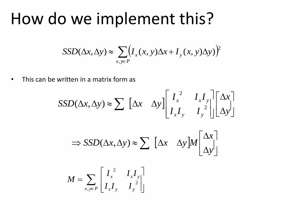
• This can be written in a matrix form as
Pyx
yx yyxIxyxIyxSSD,
2)),(),(),(
y
xMyxyxSSD ),(
How do we implement this?
y
x
III
IIIyxyxSSD
yyx
yxx ),(
2
2
2
2
, yyx
yxx
Pyx III
IIIM

• This can be written in a matrix form as
Pyx
yx yyxIxyxIyxSSD,
2)),(),(),(
y
xMyxyxSSD ),(
How do we implement this?
2
2
2
2
, yyx
yxx
yyx
yxx
Pyx III
III
III
IIIM
y
x
III
IIIyxyxSSD
yyx
yxx ),(
2
2
Alternative way to write M 2nd moment matrix
Notice that these are NOT matrix products
but pixel-wise products!

What does this matrix reveal? • First, consider an axis-aligned corner:
• This means dominant gradient directions align with 𝑥 or 𝑦 axis
• If either λ is close to 0, then this is not a corner:
• What if we have a corner that is not aligned with the image axes?
2
1
2
2
0
0
yyx
yxx
III
IIIM
2
2
2
0
00
yyx
yxx
III
IIIM
00
002
2
yyx
yxx
III
IIIM
Corner
Edge
Flat region
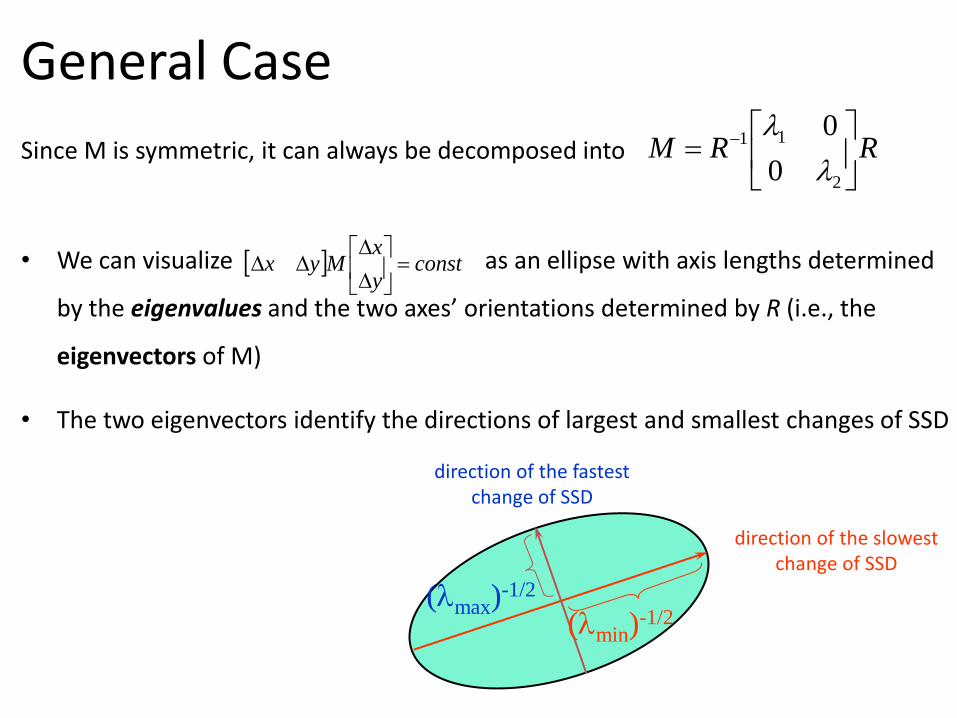
General Case
Since M is symmetric, it can always be decomposed into RRM
2
11
0
0
• We can visualize as an ellipse with axis lengths determined
by the eigenvalues and the two axes’ orientations determined by R (i.e., the
eigenvectors of M)
• The two eigenvectors identify the directions of largest and smallest changes of SSD
direction of the slowest change of SSD
direction of the fastest change of SSD
(max)-1/2
(min)-1/2
consty
xMyx
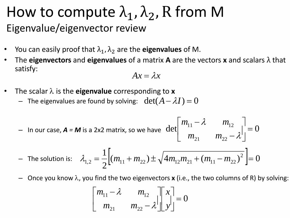
How to compute λ1, λ2, R from M Eigenvalue/eigenvector review
• You can easily proof that λ1, λ2 are the eigenvalues of M.
• The eigenvectors and eigenvalues of a matrix A are the vectors x and scalars λ that satisfy:
• The scalar is the eigenvalue corresponding to x
– The eigenvalues are found by solving:
– In our case, A = M is a 2x2 matrix, so we have
– The solution is:
– Once you know , you find the two eigenvectors x (i.e., the two columns of R) by solving:
xAx
0)det( IA
0det2221
1211
mm
mm
0)(4)(2
1 2
2211211222112,1 mmmmmm
02221
1211
y
x
mm
mm
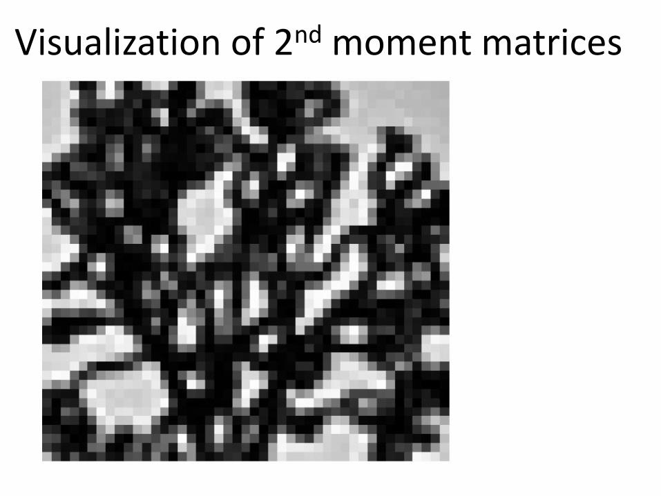
Visualization of 2nd moment matrices

Visualization of 2nd moment matrices

Interpreting the eigenvalues • Classification of image points using eigenvalues of M
• A corner can then be identified by checking whether the minimum of the two eigenvalues of M is larger than a certain user-defined threshold
⇒ R = min(1,2) > threshold
• R is called “cornerness function”
• The corner detector using this criterion is called «Shi-Tomasi» detector
1
2 “Corner”
1 and 2 are large,
⇒ R > threshold
⇒ SSD increases in all
directions
1 and 2 are small;
SSD is almost constant
in all directions
“Edge”
1 >> 2
“Edge”
2 >> 1
“Flat”
region
J. Shi and C. Tomasi (June 1994). "Good Features to Track,". 9th IEEE Conference on Computer Vision and Pattern Recognition
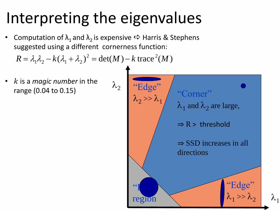
Interpreting the eigenvalues
1
2
“Edge”
1 >> 2
“Edge”
2 >> 1
“Flat”
region 1
“Corner”
1 and 2 are large,
⇒ R > threshold
⇒ SSD increases in all
directions
• Computation of λ1 and λ2 is expensive Harris & Stephens suggested using a different cornerness function:
)(trace)det()( 22
2121 MkMkR
• 𝑘 is a magic number in the range (0.04 to 0.15)

Harris Corner Detector Algorithm:
1. Compute derivatives in x and y directions (𝐼𝑥, 𝐼𝑦) e.g. with Sobel filter
2. Compute 𝐼𝑥2, 𝐼𝑦
2, 𝐼𝑥𝐼𝑦
3. Convolve 𝐼𝑥2, 𝐼𝑥
2, 𝐼𝑥𝐼𝑦 with a box filter to get 𝐼𝑥2 , 𝐼𝑦
2 , 𝐼𝑥𝐼𝑦, which are
the entries of the matrix 𝑀 (optionally use a Gaussian filter instead of a box filter to avoid aliasing and give more “weight” to the central pixels)
4. Compute Harris Corner Measure 𝑅 (according to Shi-Tomasi or Harris)
5. Find points with large corner response (𝑅 > threshold)
6. Take the points of local maxima of R
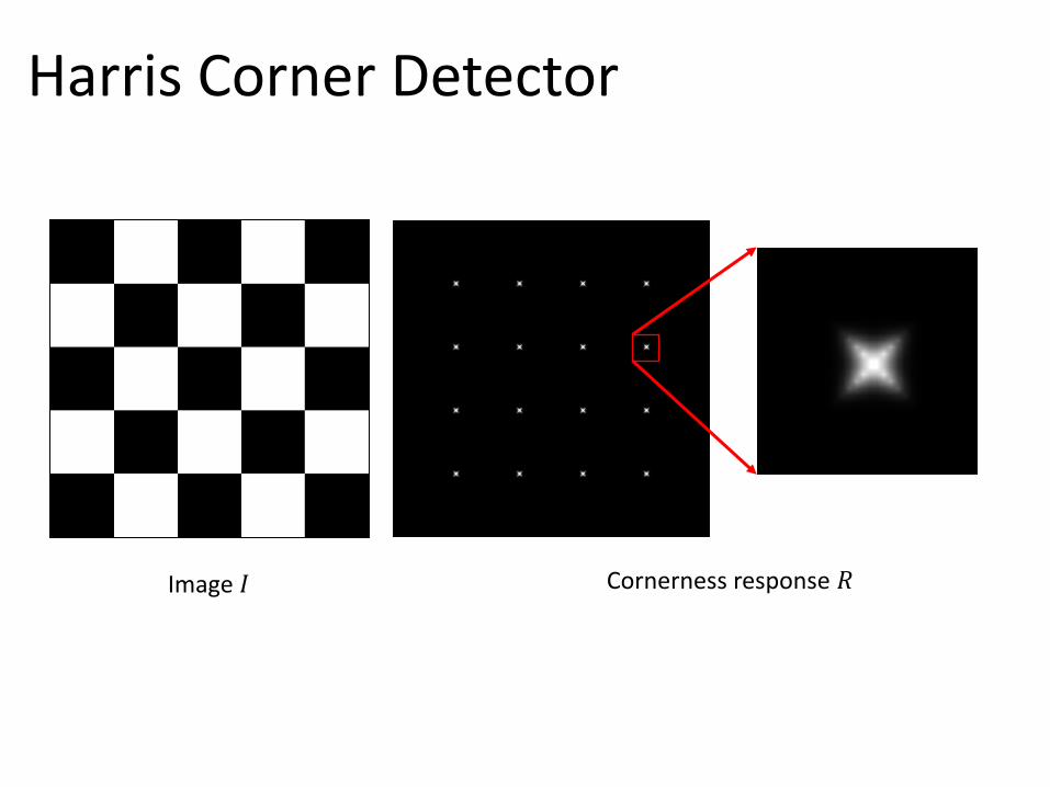
Harris Corner Detector
Image 𝐼 Cornerness response 𝑅
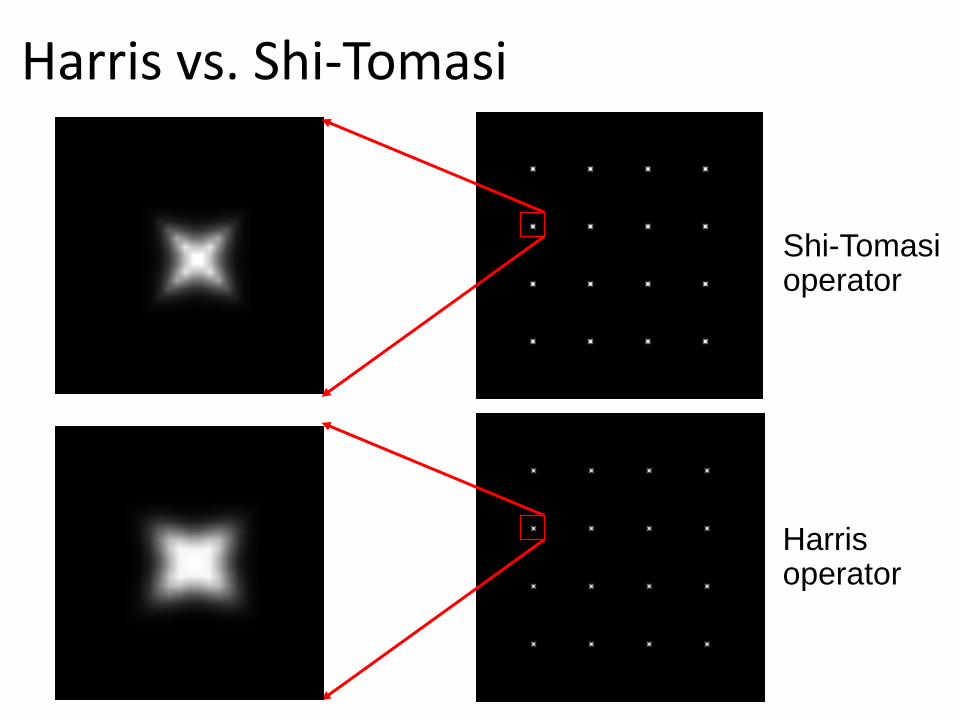
Harris vs. Shi-Tomasi
Harris operator
Shi-Tomasi operator
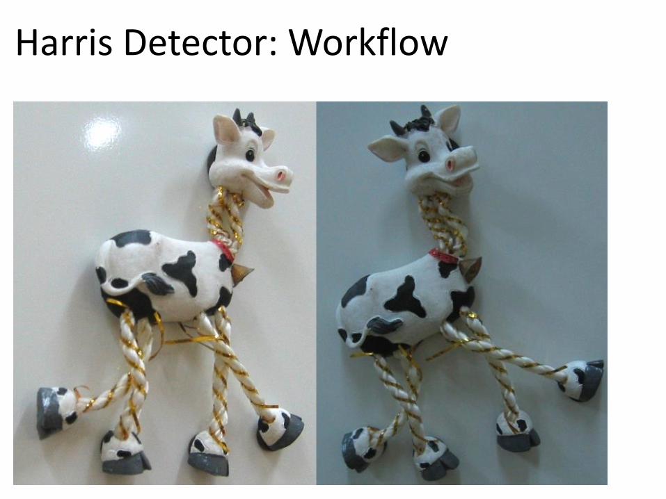
Harris Detector: Workflow
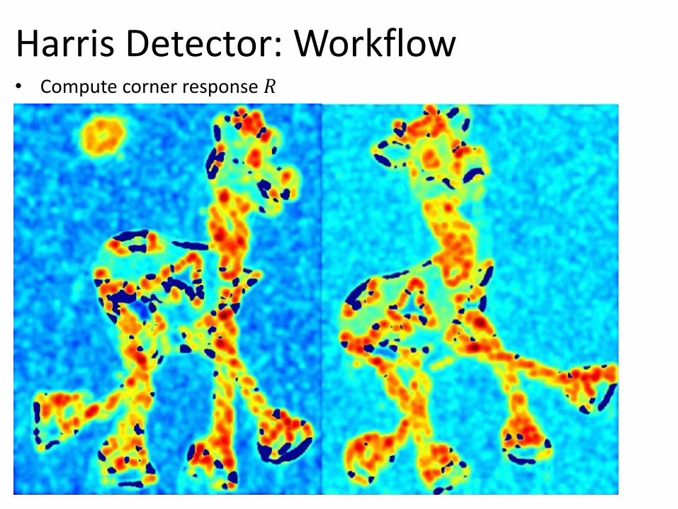
Harris Detector: Workflow • Compute corner response 𝑅
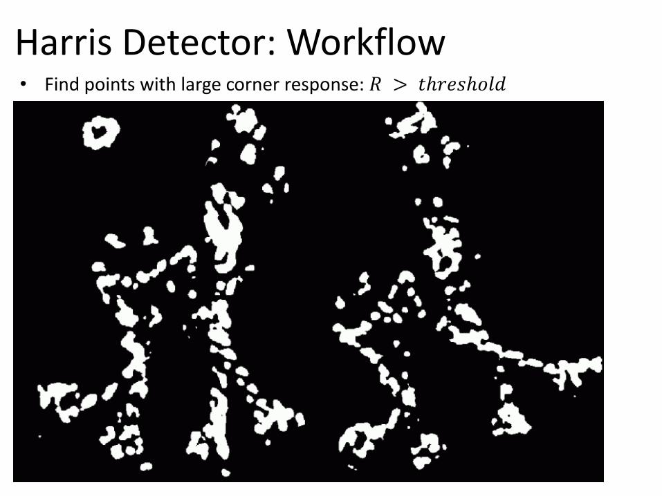
Harris Detector: Workflow • Find points with large corner response: 𝑅 > 𝑡ℎ𝑟𝑒𝑠ℎ𝑜𝑙𝑑
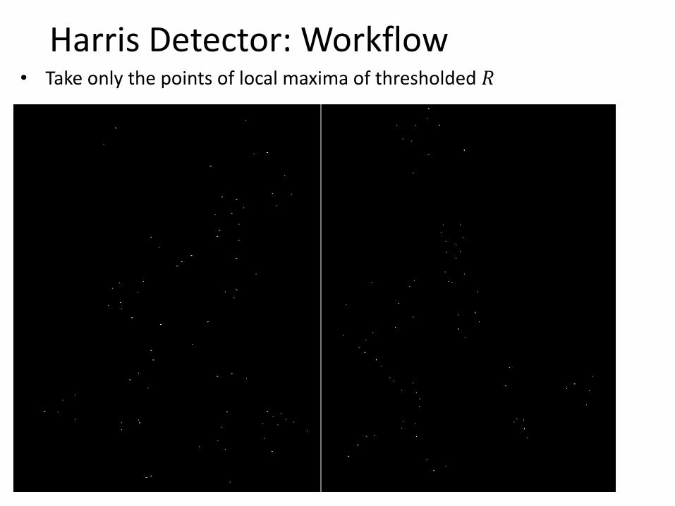
Harris Detector: Workflow • Take only the points of local maxima of thresholded 𝑅
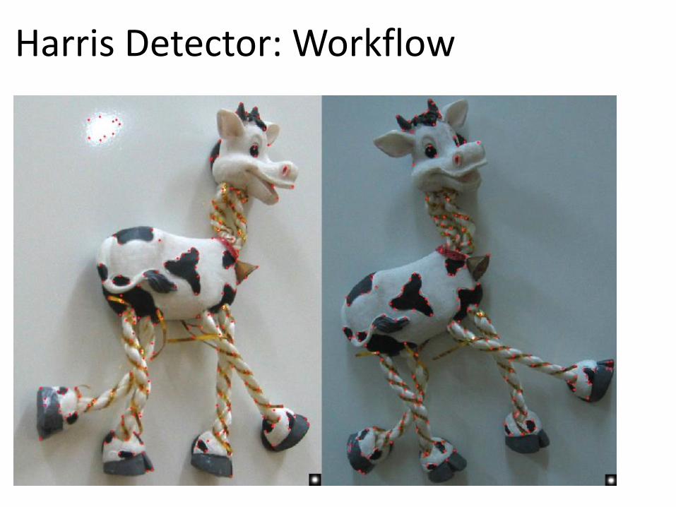
Harris Detector: Workflow

Harris Detector: Some Properties
Repeatability:
• How does the Harris detector behave to common image transformations?
• Can it re-detect the same image patches (Harris corners) when the image exhibits changes in
• Rotation,
• View-point,
• Scale (zoom),
• Illumination ?
• Solution: Identify properties of detector & adapt accordingly

Harris Detector: Some Properties
• Rotation invariance
Ellipse rotates but its shape (i.e.`, eigenvalues) remains the same
Corner response R is invariant to image rotation
Image 1 Image 2

Harris Detector: Some Properties
• But: non-invariant to image scale!
All points will be classified as edges
Corner!
Image 1 Image 2
Harris Detector: Some Properties
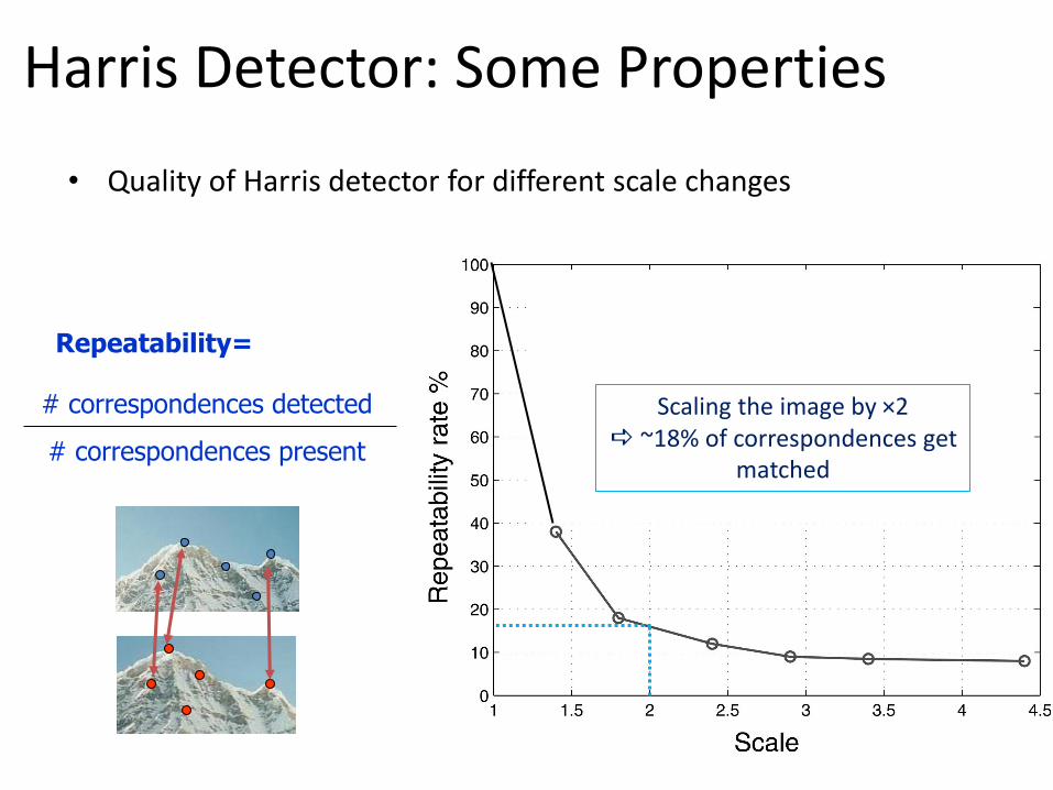
• Quality of Harris detector for different scale changes
Repeatability=
# correspondences detected
# correspondences present
Scaling the image by ×2 ~18% of correspondences get
matched

Image 1 Image 2
Scale changes
• How can we match image patches corresponding to the same feature but belonging to images taken at different scales?
– Possible solution: rescale the patch!
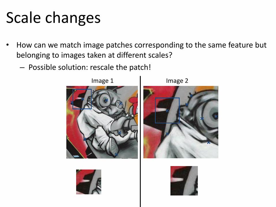
Image 1 Image 2
Scale changes
• How can we match image patches corresponding to the same feature but belonging to images taken at different scales?
– Possible solution: rescale the patch!
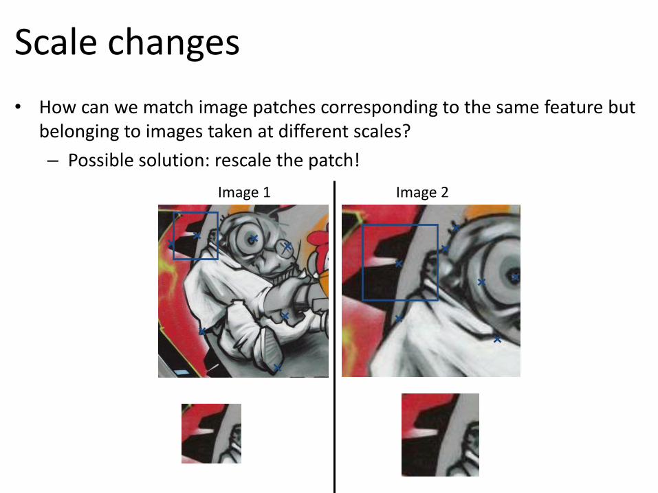
Scale changes
• How can we match image patches corresponding to the same feature but belonging to images taken at different scales?
– Possible solution: rescale the patch!
Image 1 Image 2

Image 1 Image 2
Scale changes
• How can we match image patches corresponding to the same feature but belonging to images taken at different scales?
– Possible solution: rescale the patch!
Scale changes
• Scale search is time consuming (needs to be done individually for all patches in one image)
• Possible solution: assign each feature its own “scale” (i.e., size).
– What’s the optimal scale (i.e., size) of the patch?
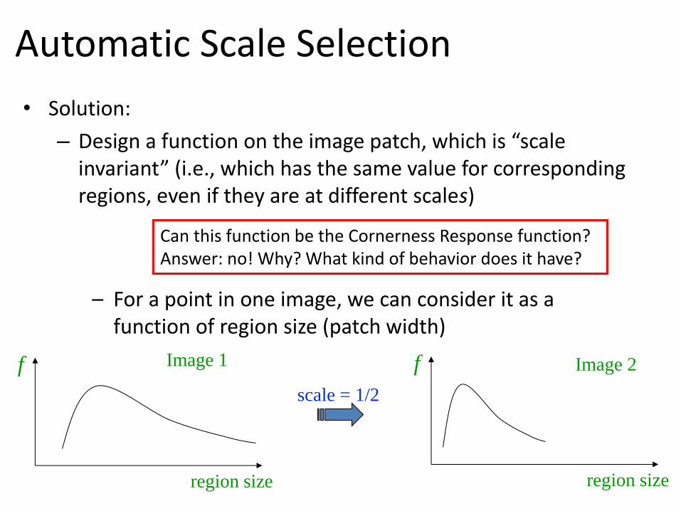
• Solution:
– Design a function on the image patch, which is “scale invariant” (i.e., which has the same value for corresponding regions, even if they are at different scales)
Can this function be the Cornerness Response function? Answer: no! Why? What kind of behavior does it have?
scale = 1/2
– For a point in one image, we can consider it as a function of region size (patch width)
f
region size
Image 1 f
region size
Image 2
Automatic Scale Selection

• Common approach:
scale = 1/2
f
region size
Image 1 f
region size
Image 2
Take a local maximum of this function
Observation: region size, for which the maximum is achieved, should be invariant to image scale.
s1 s2
Important: this scale invariant region size is found in each image independently!
Automatic Scale Selection

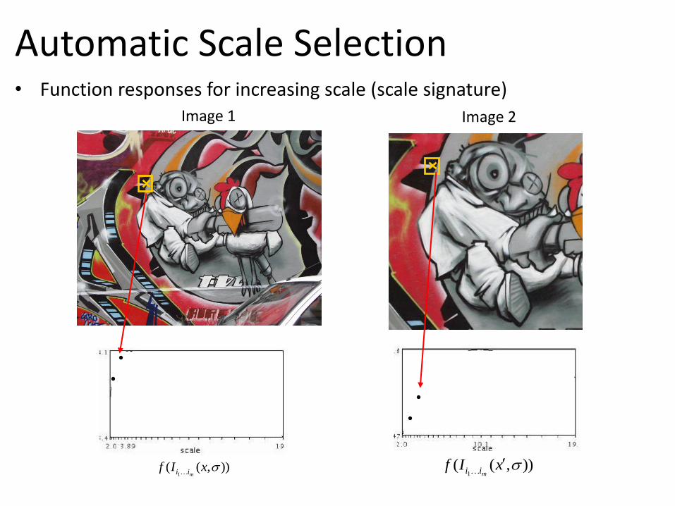
Automatic Scale Selection • Function responses for increasing scale (scale signature)
)),((1
xIfmii
)),((1
xIfmii
Image 1 Image 2
Automatic Scale Selection
)),((1
xIfmii
)),((1
xIfmii
• Function responses for increasing scale (scale signature) Image 1 Image 2

Automatic Scale Selection
)),((1
xIfmii
)),((1
xIfmii
• Function responses for increasing scale (scale signature) Image 1 Image 2

Automatic Scale Selection
)),((1
xIfmii
)),((1
xIfmii
• Function responses for increasing scale (scale signature) Image 1 Image 2

Automatic Scale Selection
)),((1
xIfmii
)),((1
xIfmii
• Function responses for increasing scale (scale signature) Image 1 Image 2

Automatic Scale Selection
)),((1
xIfmii
)),((1
xIfmii
• Function responses for increasing scale (scale signature) Image 1 Image 2
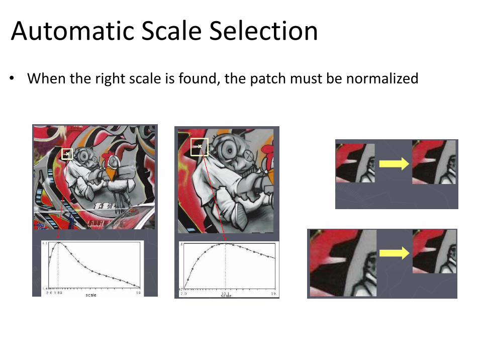
Automatic Scale Selection
• When the right scale is found, the patch must be normalized

Scale Invariant Detection: Robustness
• A “good” function for scale detection should have a single & sharp peak
• Sharp, local intensity changes are good regions to monitor in order to identify the scale
Blobs and corners are the ideal locations!
I
region size
bad
I
region size
bad
I
region size
Good !
A cornerness response function would exhibit this
“flat ”behavior, why?

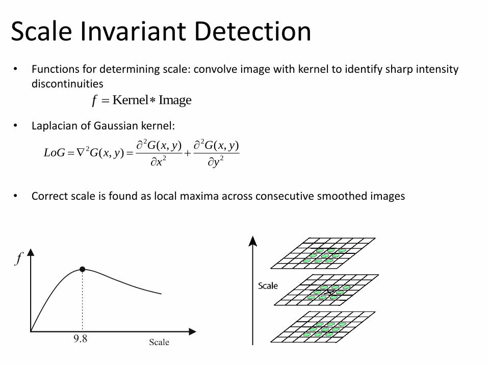
Scale Invariant Detection • Functions for determining scale: convolve image with kernel to identify sharp intensity
discontinuities
• Laplacian of Gaussian kernel:
• Correct scale is found as local maxima across consecutive smoothed images
Kernel Imagef
2
2
2
22 ),(),(
),(y
yxG
x
yxGyxGLoG
2
3
4
Scale
Scale Invariant Detection • Functions for determining scale: convolve image with kernel to identify sharp intensity
discontinuities
• Laplacian of Gaussian kernel:
• Correct scale is found as local maxima across consecutive smoothed images
Kernel Imagef
2
2
2
22 ),(),(
),(y
yxG
x
yxGyxGLoG
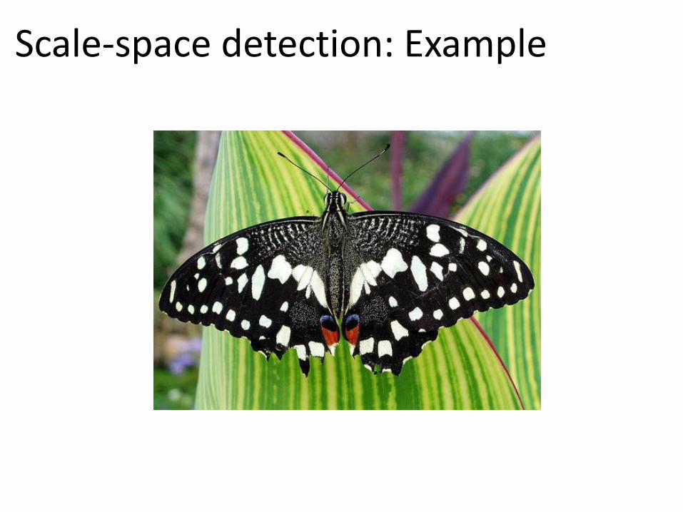
Scale-space detection: Example
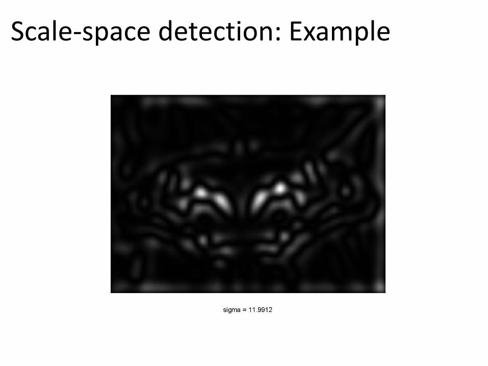
Scale-space detection: Example
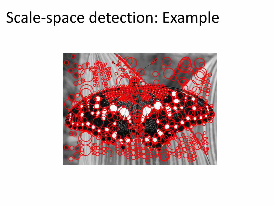
Scale-space detection: Example

Scale Invariant Detectors
• Experimental evaluation of detectors w.r.t. scale change
Repeatability=
# correspondences detected
# correspondences present
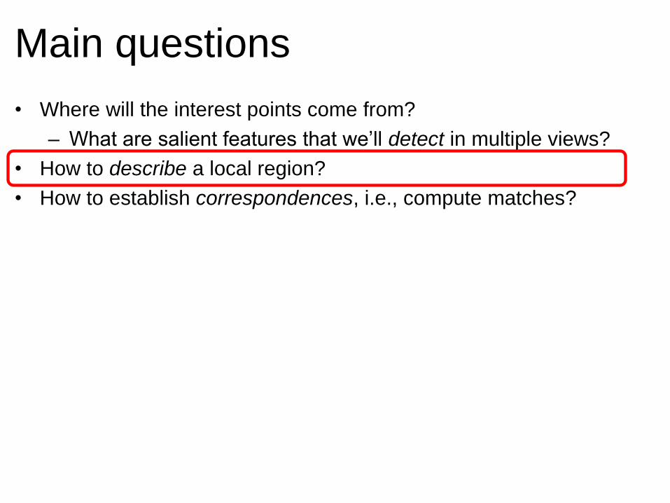
Main questions
• Where will the interest points come from?
– What are salient features that we’ll detect in multiple views?
• How to describe a local region?
• How to establish correspondences, i.e., compute matches?
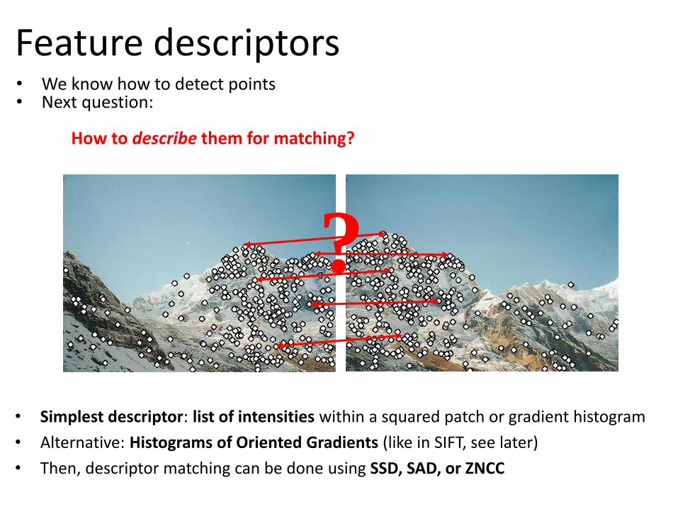
• We know how to detect points • Next question:
How to describe them for matching?
?
• Simplest descriptor: list of intensities within a squared patch or gradient histogram
• Alternative: Histograms of Oriented Gradients (like in SIFT, see later)
• Then, descriptor matching can be done using SSD, SAD, or ZNCC
Feature descriptors
Feature descriptors
• We’d like to find the same features regardless of the transformation (rotation, scale, view point, and illumination)
– Most feature methods are designed to be invariant to
• translation,
• 2D rotation,
• scale
– Some of them can also handle
• Small view-point invariance (3D rotation) (e.g., SIFT works up to about 60 degrees)
• Linear illumination changes
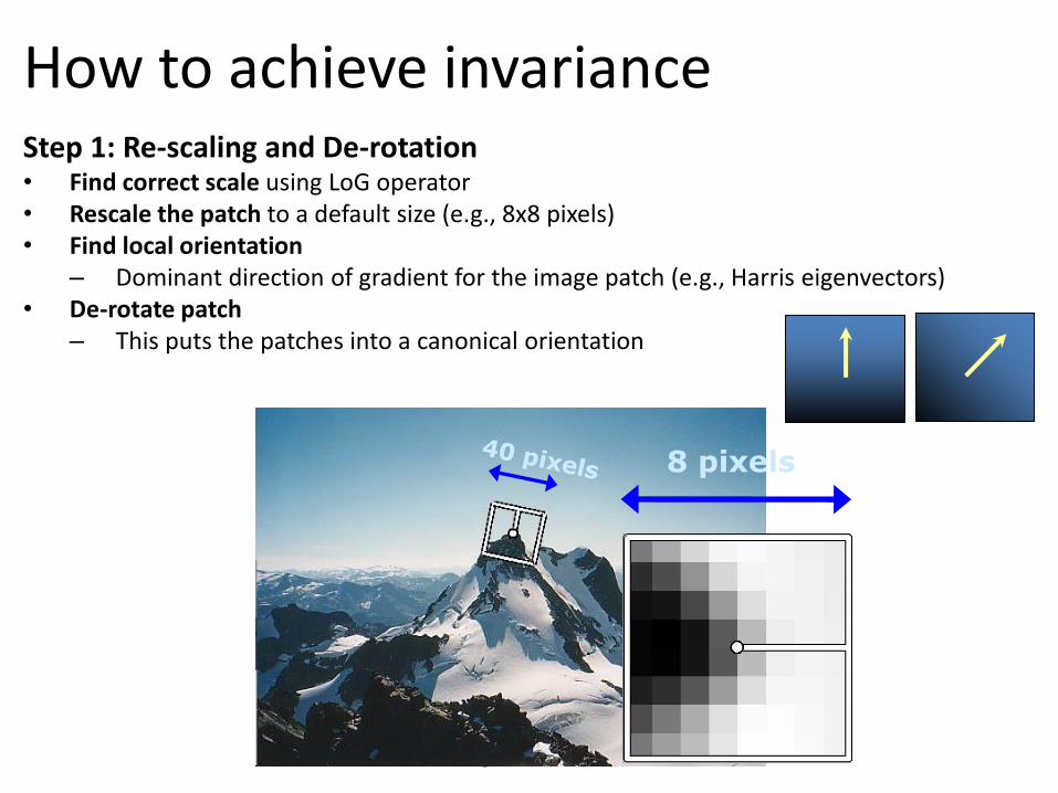
How to achieve invariance
CSE 576: Computer Vision
8 pixels
Step 1: Re-scaling and De-rotation • Find correct scale using LoG operator • Rescale the patch to a default size (e.g., 8x8 pixels) • Find local orientation
– Dominant direction of gradient for the image patch (e.g., Harris eigenvectors) • De-rotate patch
– This puts the patches into a canonical orientation

How to achieve invariance Step 2: Affine Un-warping (to achieve slight view-point invariance) • The second moment matrix M can be used to identify the two directions of fastest and
slowest change of intensity around the feature.
• Out of these two directions, an elliptic patch is extracted at the scale computed by with the LoG operator.
• The region inside the ellipse is normalized to a circular one
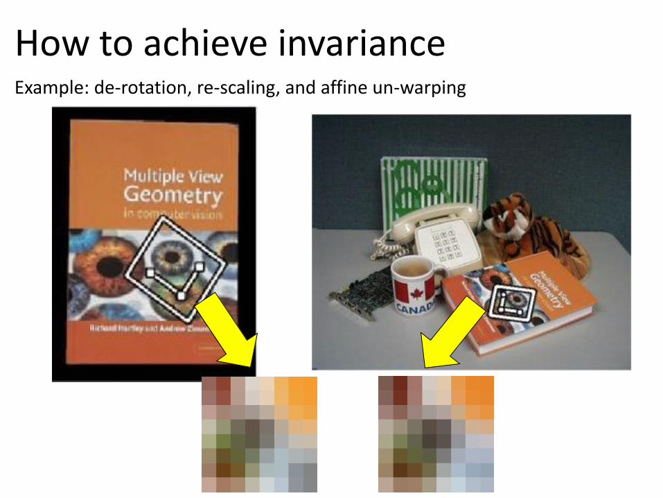
Example: de-rotation, re-scaling, and affine un-warping
How to achieve invariance

Feature descriptors
• Disadvantage of patches as descriptors:
– Very small errors in rotation, scale, view-point, and illumination can affect matching score significantly
– Computationally expensive (need to unwarp every patch)
• Better solution today: build descriptors from Histograms of Oriented Gradients (HOGs)
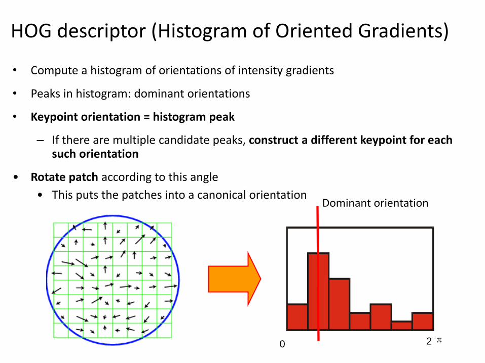
HOG descriptor (Histogram of Oriented Gradients)
• Compute a histogram of orientations of intensity gradients
• Peaks in histogram: dominant orientations
• Keypoint orientation = histogram peak
– If there are multiple candidate peaks, construct a different keypoint for each such orientation
• Rotate patch according to this angle
• This puts the patches into a canonical orientation
0 2 p
Dominant orientation
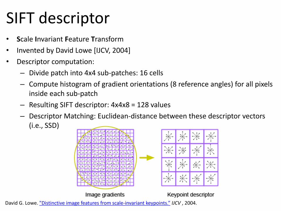
• Scale Invariant Feature Transform
• Invented by David Lowe [IJCV, 2004]
• Descriptor computation:
– Divide patch into 4x4 sub-patches: 16 cells
– Compute histogram of gradient orientations (8 reference angles) for all pixels inside each sub-patch
– Resulting SIFT descriptor: 4x4x8 = 128 values
– Descriptor Matching: Euclidean-distance between these descriptor vectors (i.e., SSD)
SIFT descriptor
David G. Lowe. "Distinctive image features from scale-invariant keypoints.” IJCV , 2004.
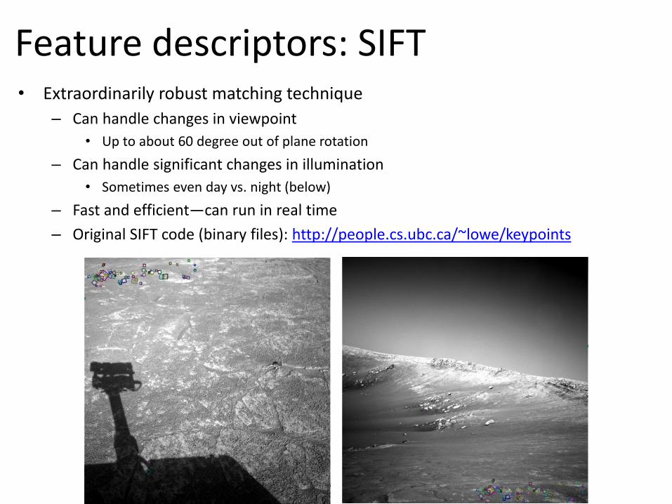
Feature descriptors: SIFT • Extraordinarily robust matching technique
– Can handle changes in viewpoint
• Up to about 60 degree out of plane rotation
– Can handle significant changes in illumination
• Sometimes even day vs. night (below)
– Fast and efficient—can run in real time
– Original SIFT code (binary files): http://people.cs.ubc.ca/~lowe/keypoints
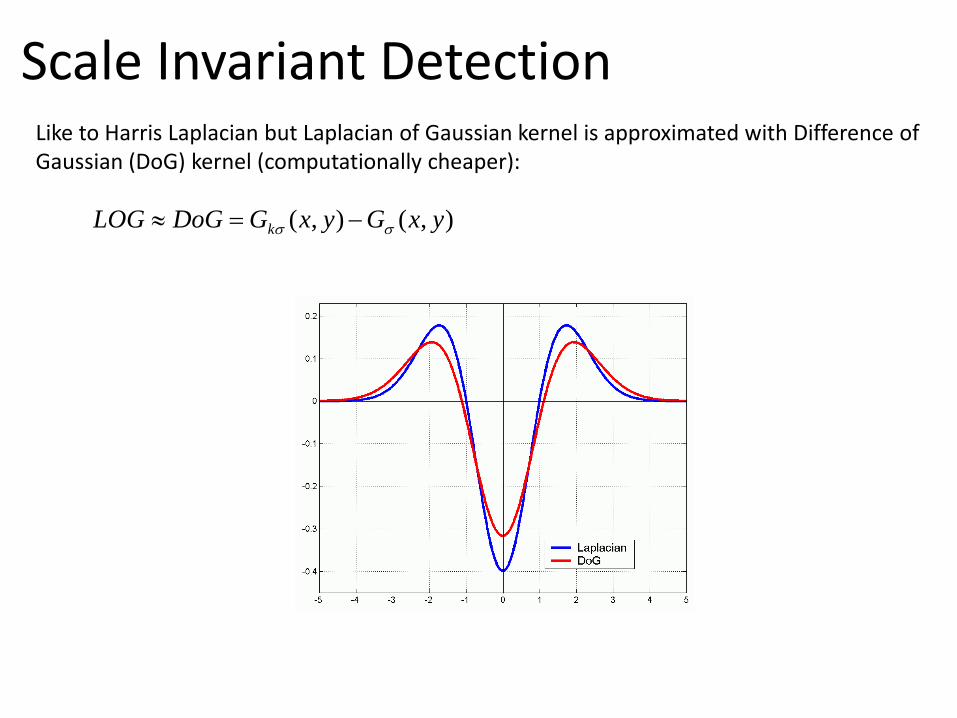
Scale Invariant Detection Like to Harris Laplacian but Laplacian of Gaussian kernel is approximated with Difference of Gaussian (DoG) kernel (computationally cheaper):
),(),( yxGyxGDoGLOG k

SIFT detector (location + scale) SIFT keypoints: local extrema in the DoG pyramid

SIFT Features: Summary SIFT: Scale Invariant Feature Transform [Lowe, IJCV 2004]
An approach to detect and describe regions of interest in an image.
SIFT features are reasonably invariant to changes in rotation, scaling, and small changes in viewpoint and illumination
Computationally a bit costly (10 Hz)
Expensive steps are the scale detection and descriptor extraction
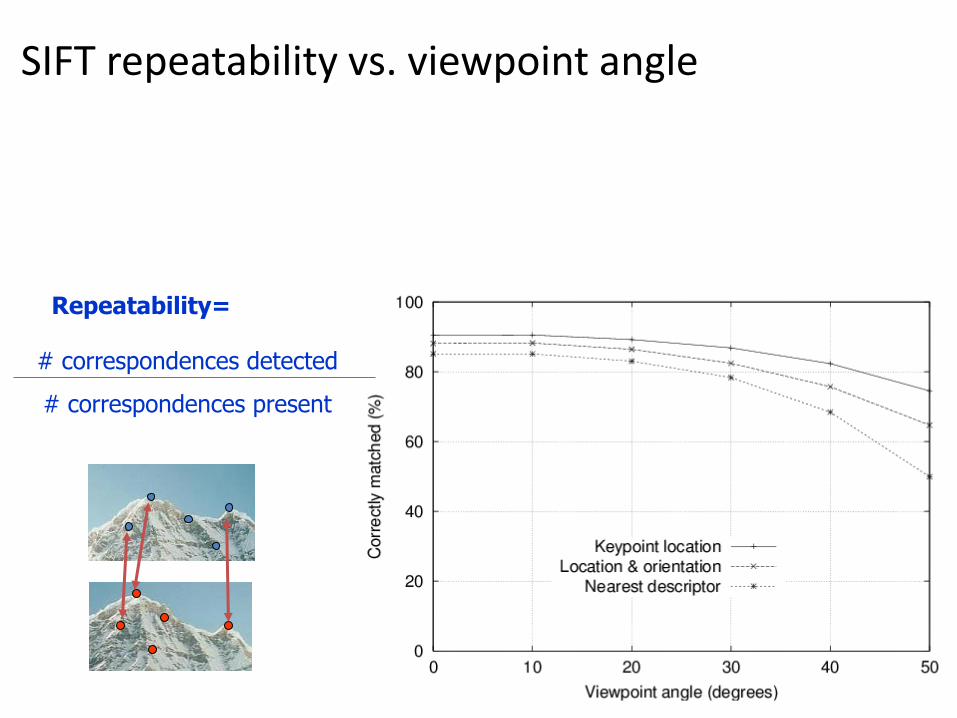
SIFT repeatability vs. viewpoint angle
Repeatability=
# correspondences detected
# correspondences present

SIFT repeatability vs. Scale
Repeatability=
# correspondences detected
# correspondences present
Harris SIFT

How many parameters are used to define a
SIFT feature?
• Descriptor: 128 parameters
• Location (pixel coordinates of the center of the patch): 2D vector
• Size (i.e., scale) of the patch: 1 scalar value
• Orientation (i.e., angle of the patch): 1 scalar value
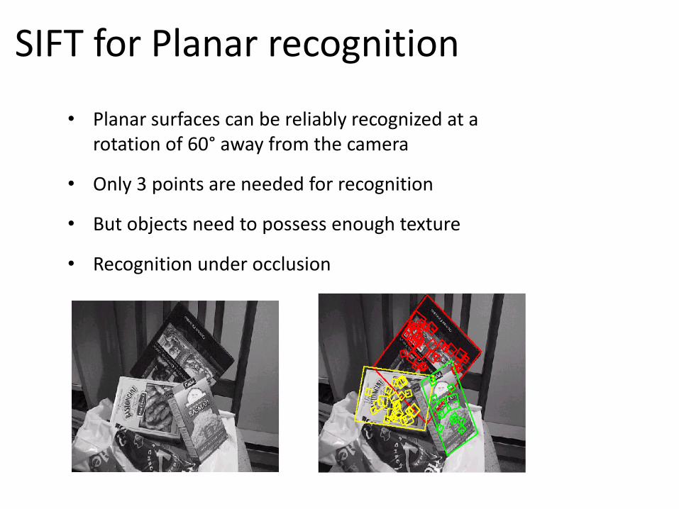
SIFT for Planar recognition
• Planar surfaces can be reliably recognized at a rotation of 60° away from the camera
• Only 3 points are needed for recognition
• But objects need to possess enough texture
• Recognition under occlusion

SIFT for Panorama Stitching
[M. Brown and D. G. Lowe. Recognising Panoramas. ICCV 2003]
AutoStitch: http://matthewalunbrown.com/autostitch/autostitch.html

Main questions
• Where will the interest points come from?
– What are salient features that we’ll detect in multiple views?
• How to describe a local region?
• How to establish correspondences, i.e., compute matches?
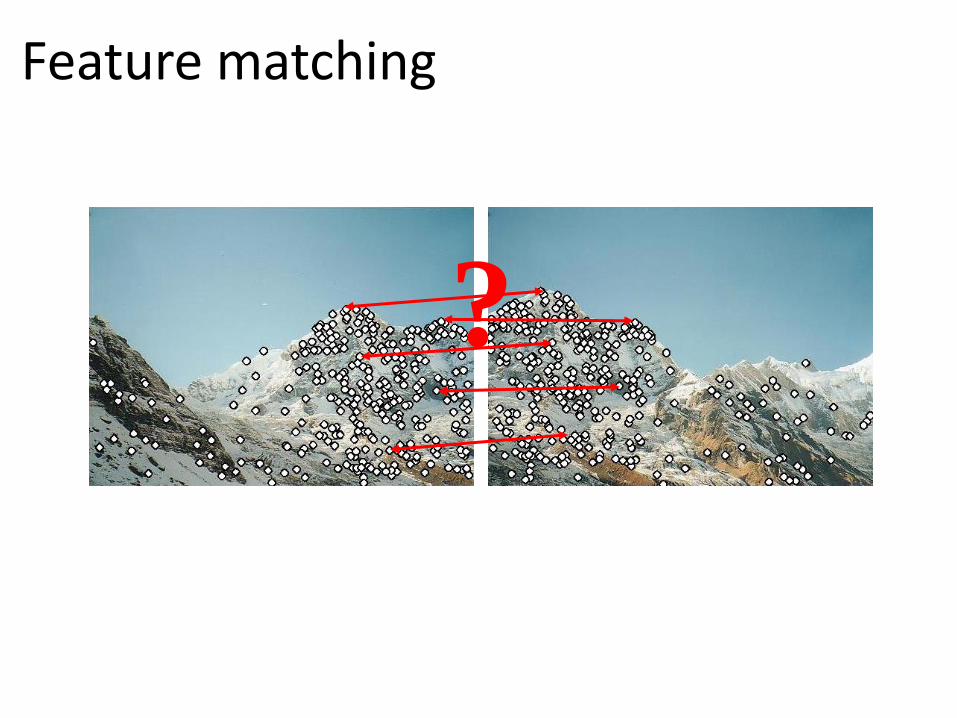
Feature matching
?

Feature matching
• Given a feature in 𝐼1, how to find the best match in 𝐼2?
1. Define distance function that compares two descriptors
SSD (also called L2 norm)
SAD
ZNCC
2. Brute-force matching: Test all the features in 𝐼2, find the one with min distance
• Problem with distance: can give good scores to very ambiguous (bad) matches!
• Better approach: ratio distance = d(f1, f2) / d(f1, f2’) < Threshold (e.g., 0.8)
• f2 is best match to f1 in I2
• f2’ is 2nd best match to f1 in I2
• gives small values for ambiguous matches
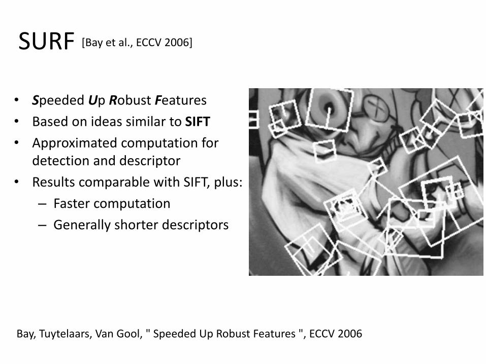
SURF
• Speeded Up Robust Features
• Based on ideas similar to SIFT
• Approximated computation for detection and descriptor
• Results comparable with SIFT, plus:
– Faster computation
– Generally shorter descriptors
[Bay et al., ECCV 2006]
Bay, Tuytelaars, Van Gool, " Speeded Up Robust Features ", ECCV 2006
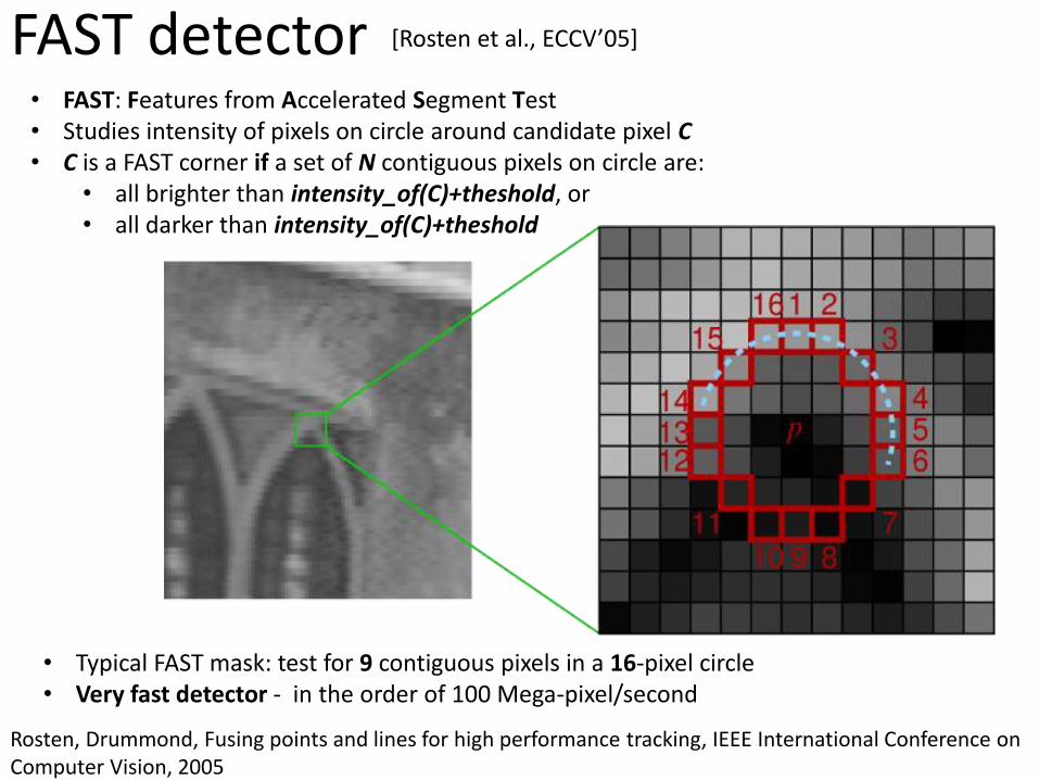
FAST detector [Rosten et al., ECCV’05]
• FAST: Features from Accelerated Segment Test • Studies intensity of pixels on circle around candidate pixel C • C is a FAST corner if a set of N contiguous pixels on circle are:
• all brighter than intensity_of(C)+theshold, or • all darker than intensity_of(C)+theshold
• Typical FAST mask: test for 9 contiguous pixels in a 16-pixel circle • Very fast detector - in the order of 100 Mega-pixel/second
Rosten, Drummond, Fusing points and lines for high performance tracking, IEEE International Conference on Computer Vision, 2005
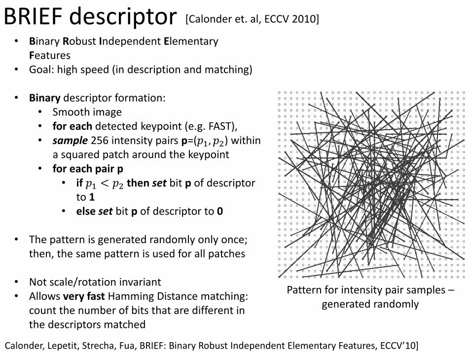
BRIEF descriptor [Calonder et. al, ECCV 2010]
Pattern for intensity pair samples – generated randomly
• Binary Robust Independent Elementary Features
• Goal: high speed (in description and matching)
• Binary descriptor formation: • Smooth image • for each detected keypoint (e.g. FAST), • sample 256 intensity pairs p=(𝑝1, 𝑝2) within
a squared patch around the keypoint • for each pair p
• if 𝑝1 < 𝑝2 then set bit p of descriptor to 1
• else set bit p of descriptor to 0
• The pattern is generated randomly only once; then, the same pattern is used for all patches
• Not scale/rotation invariant • Allows very fast Hamming Distance matching:
count the number of bits that are different in the descriptors matched
Calonder, Lepetit, Strecha, Fua, BRIEF: Binary Robust Independent Elementary Features, ECCV’10]

• Oriented FAST and Rotated BRIEF
• Alterative to SIFT or SURF, designed for fast computation
• Keypoint detector based on FAST
• BRIEF descriptors are steered according to keypoint orientation (to provide rotation invariance)
• Good Binary features are learned by minimizing the correlation on a set of training patches.
ORB descriptor [Rublee et al., ICCV 2011]

BRISK descriptor [Leutenegger, Chli, Siegwart, ICCV 2011]
• Binary Robust Invariant Scalable Keypoints • Detect corners in scale-space using FAST • Rotation and scale invariant
• Binary, formed by pairwise intensity comparisons (like BRIEF)
• Pattern defines intensity comparisons in the keypoint neighborhood
• Red circles: size of the smoothing kernel applied
• Blue circles: smoothed pixel value used • Compare short- and long-distance pairs
for orientation assignment & descriptor formation
• Detection and descriptor speed: ~10 times faster than SURF
• Slower than BRIEF, but scale- and rotation- invariant

Summary (things to remember) • Point feature detection
– Properties and invariance to transformations
• Challenges: rotation, scale, view-point, and illumination changes
– Extraction
• Harris and Shi-Tomasi
– Rotation invariance
– Scale invariance: Harris Laplacian
– Descriptor
• Intensity patches
– How to make them invariant to transformations: rotation, scale, illumination, and view-point (affine)
• Better solution: Histogram of oriented gradients: SIFT descriptor
– Matching
• SSD, SAD, ZNCC, ratio 1st /2nd closest descriptor
– Depending on the task, you may want to trade repeatability and robustness for speed: approximated solutions, combinations of efficient detectors and descriptors.
• Fast corner detector: FAST;
• Keypoint descriptors faster than SIFT: SURF, BRIEF, ORB, BRISK
• Autonomous Mobile Robot book chapter 4.5
• Szeliski book chapters 4.3.2 and 4.1


