
1
EE4900/EE6420 Digital Communications Suketu Naik
EE4900/EE6420: Digital Communications
Lecture 5
Review
of Probability
Theory

2
EE4900/EE6420 Digital Communications Suketu Naik
Block Diagrams of Communication System
Digital Communication System
Informatio
n (sound,
video, text,
data, …)
Transducer &
A/D ConverterModulator
Source
Encoder
Channel
Encoder
Tx RF
System
Output
Signal
D/A Converter
and/or output
transducer
DemodulatorSource
Decoder
Channel
Decoder
Rx RF
System
Channel

3
EE4900/EE6420 Digital Communications Suketu Naik
Why Study Probability in Dig. Comm?
Nature of noise is random
Nature of information is random
Randomness affects the performance of comm. system
When message signal is transmitted through a channel
(wired/wireless) it gets corrupted by noise
To recover the message signal, we use probability theory
for estimation
Transmitter Receiver
Channel
(Wire,
Air,
Water,
Space)
Noise

4
EE4900/EE6420 Digital Communications Suketu Naik
What is Noise?
Noise the phenomena that is generated by,
Electronics in Transmitter and Receiver
The medium or channel which the information passes
through
Noise can be characterized by,
Random variables and processes (mathematical models)
Random=Unpredictable
Transmitter Receiver
Channel
(Wire,
Air,
Water,
Space)
Noise
Noise Noise
5
EE4900/EE6420 Digital Communications Suketu Naik
Sample Space Ω and Measure P
Noise aka randomness produces random outcomes: how to
characterize the random outcome based on an event?
The set of all possible random outcomes is called
Samples Space Ω
Let an outcome 𝛚 ∈ 𝛀 Let an event A = subset of Ω; 𝐀 ⊂ 𝛀 Let a set of all possible events be ε; ε = event space
Let a measure P map members of ε to the real interval
[0, 1]
Measure P is a probability measure that characterizes
the randomness
(𝛀, ε, P) defines the probability space
6
EE4900/EE6420 Digital Communications Suketu Naik
Simple Examples
Example 4.1.1: Coin Toss
Outcomes: Heads=H, Tails=T
What is sample space 𝛀 ? 𝛀 = 𝐇,𝐓 What is the event space ε? 𝛆 = 𝟎, 𝐇 , 𝐓 , 𝐇, 𝐓 What is the probability measure P for the above event
space?
𝐏 𝟎 = 𝟎
𝐏 𝐇 = 𝟏/𝟐
𝐏 𝐓 = 𝟏/𝟐
𝐏 𝐇, 𝐓 = 𝟏
0% Probability that neither heads or tails happen
50% Probability that heads will happen
50% Probability that tails will happen
100% Probability that either heads or tails
will happen

7
EE4900/EE6420 Digital Communications Suketu Naik
Conditional Probability
Bayes’ Rule
Toss the coin twice. What is P(H|T)=What is the
probability that we get Heads given that Tails has
happened?
Sample Space 𝛀 = 𝐓𝐓, 𝐓𝐇,𝐇𝐓,𝐇𝐇
Bayes’ Rule: 𝑷(𝑯|𝑻) =𝑷(𝑻|𝑯)𝑷(𝑯)
𝑷(𝑻)
P(H)=1/2, P(T)=1/2 => P(H|T)=P(T|H)
P(T|H)=P(T∩H)/P(H)=(1/4) /(1/2)=1/2
Recall that
𝑷(𝑨|𝑩) =𝑷(𝑨 ∩ 𝑩)
𝑷(𝑩)
8
EE4900/EE6420 Digital Communications Suketu Naik
Conditional Probability
Die Example
Die Events=S=1,2,3,4,5,6= Total of 6 possible outcomes
A=odds=1, 3, 5, B=1,2,3
What is P(A|B)=What is the probability of A given that
1, 2, 3 have already been thrown?
Answer: P(A|B)=P(A ∩ B)/P(B)
P(A ∩ B)=?
1) P(A)=|1,3,5|/6=3/6; P(B)=|1,2,3|/6=3/6
2) Now A ∩ B = 1, 3 so P(A ∩ B)=2/6
P(A|B)= (2/6)/(3/6)=1/3=30% chance of getting an odd
number given that 1,2,3 has occurred
Ref:
https://www.probabilitycourse.com/chapter1/1_4_0_conditional_probability.php

9
EE4900/EE6420 Digital Communications Suketu Naik
Random Variable
What is Random Variable?
Let Random Variable X(ω) map the sample space Ω to
real line R
Note that the random variable X(ω) is a point 𝐱 ∈ 𝐑 for
each outcome ω
Note that the
outcome
is single
element

10
EE4900/EE6420 Digital Communications Suketu Naik
Random Variable
Note that now
the outcome
is within a set B x= the end point within this interval B on the real line
with open interval B=(-∞, x]
Probability measure P of the interval B = function of end
point x = Cumulative Distribution Function = CDF = FX(x)

11
EE4900/EE6420 Digital Communications Suketu Naik
Random Variable and its CDF
We can use the CDF to calculate the probability P that a
random variable X is less than a real value x

12
EE4900/EE6420 Digital Communications Suketu Naik
Probability Density Function
Probability measure P of the interval B = function of end
point x = Cumulative Distribution Function = FX(x)
Derivative of the FX(x)= fX(x)=Probability Density
Function = PDF
For discrete random variables, FX(x) has stair-step
shape; fX(x) is defined by impulse functions
Example 4.1.3: Figure
Example 4.1.4: Figure
Either CDF or PDF will quantify the probability that X maps to x
13
EE4900/EE6420 Digital Communications Suketu Naik
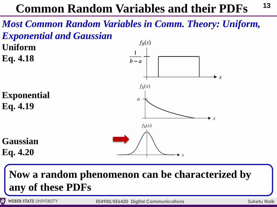
Common Random Variables and their PDFs
Most Common Random Variables in Comm. Theory: Uniform,
Exponential and Gaussian
Uniform
Eq. 4.18
Exponential
Eq. 4.19
Gaussian
Eq. 4.20
Now a random phenomenon can be characterized by
any of these PDFs

14
EE4900/EE6420 Digital Communications Suketu Naik
Gaussian (Normal) Random Variable
Gaussian (Normal) Random Variable is most useful in Dig.
Comm.
It can be used to represent
1) noise in the communication system and channel
2) random fluctuation of received voltage (message) in
cellular systems, smart-phones, wireless routers, etc.
Gaussian Random Variable
Eq. 4.20
Note that Gaussian R.V. has PDF that is completely defined
by its mean μ and its variance σ2 (σ = standard deviation)

15
EE4900/EE6420 Digital Communications Suketu Naik
Gaussian (Normal) Random Variable
Gaussian Distribution
One
Standard
Deviation
16
EE4900/EE6420 Digital Communications Suketu Naik
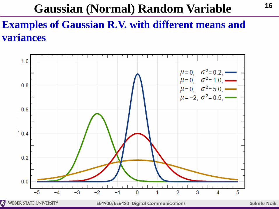
Gaussian (Normal) Random Variable
Examples of Gaussian R.V. with different means and
variances

17
EE4900/EE6420 Digital Communications Suketu Naik
Gaussian (Normal) Random Variable
PDF: Eq. 4.21
Mean: Eq. 4.22
Variance: Eq. 4.23
Common Notation: Eq. 4.24
CDF (Cumulative Distribution Function): Eq. 4.25
CDF does not have closed form: it must be evaluated
numerically as an approximation
One of the most commonly used approximations is Error
Function, erf(x)
erf(x): Eq.4.26
18
EE4900/EE6420 Digital Communications Suketu Naik
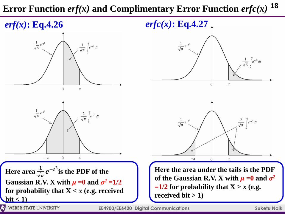
Error Function erf(x) and Complimentary Error Function erfc(x)
erf(x): Eq.4.26 erfc(x): Eq.4.27
Here area 𝟏
√𝝅𝒆−𝒕
𝟐is the PDF of the
Gaussian R.V. X with μ =0 and σ2 =1/2
for probability that X < x (e.g. received
bit < 1)
Here the area under the tails is the PDF
of the Gaussian R.V. X with μ =0 and σ2
=1/2 for probability that X > x (e.g.
received bit > 1)

19
EE4900/EE6420 Digital Communications Suketu Naik
Q function: Q(x)
𝑸(𝒙) =𝟏
𝟐𝒆𝒓𝒇𝒄(
𝒙
√𝟐) & Eq. 4.28
Upper tails of the Q function define the probability that
X (the Gaussian Random Variable) > x (the real value)
Matlab Script:
function y = Q(x)
y=0.5*erfc(x/sqrt(2));
20
EE4900/EE6420 Digital Communications Suketu Naik
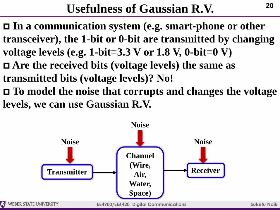
Usefulness of Gaussian R.V.
Transmitter Receiver
Channel
(Wire,
Air,
Water,
Space)
Noise
Noise Noise
In a communication system (e.g. smart-phone or other
transceiver), the 1-bit or 0-bit are transmitted by changing
voltage levels (e.g. 1-bit=3.3 V or 1.8 V, 0-bit=0 V)
Are the received bits (voltage levels) the same as
transmitted bits (voltage levels)? No!
To model the noise that corrupts and changes the voltage
levels, we can use Gaussian R.V.

21
EE4900/EE6420 Digital Communications Suketu Naik
Two Random Variables and their joint PDFs
We have focused on one random variable which may
represent the randomness of a voltage level (1-bit or 0-
bit): For example, we might say that we are 90% (prob.
measure P) sure that the voltage is within +/-0.1 V
(standard deviation σ) of 3.3 V (mean μ) level.
The above is a statistical description as opposed to
deterministic description: e.g. voltage is exactly 3.3 V
In communication systems (e.g. transceivers), 0-bit and
1-bit are often transmitted together (e.g. QPSK
modulation): now we need to look at joint probability of
two random variables

22
EE4900/EE6420 Digital Communications Suketu Naik
Two Random Variables and their joint PDFs
Let’s say that we have two random variables: X (corrupted
1-bit voltage level) and Y (corrupted 0-bit voltage level)
We look at Covariance to understand the relationship
between X with mean μX and Y with mean μY
Mean of single R.V.: Eq. 4.22
Correlation function, corr(X,Y): Eq. 4.31-4.32
Covariance function, cov(X,Y): Eq. 4.34-4.35
If Covariance is,
positive: 1) high prob. that large values of X occur with large
values of Y (both 1-bit and 0-bit count is pretty high)
2) high prob. That small values of X occur with small
values of Y (both 1-bit and 0-bit count is pretty low)
negative: high prob. that large values of X occur with small
values of Y (1-bit is more likely than 0-bit)
zero: X & Y are uncorrelated (Eq. 4.33, the 1-bit and 0-bit
can be decoded independently)

23
EE4900/EE6420 Digital Communications Suketu Naik
Functions of Random Variables
In the analysis of communication systems, functions of
random variables are often encountered
Let’s say Z ~ N(μZ ,σZ2) is a random variable that is a
function of X ~ N(μX ,σX2) and Y ~ N(μY ,σY
2)
1) Z=aX+bY, μZ= aμX + bμY and σZ2 = aσX
2 + bσY2
1) Z=X2+Y2, μZ= aμX + bμY and σZ2 = aσX
2 + bσY2
1) Others: p.193-194

24
EE4900/EE6420 Digital Communications Suketu Naik
Multivariate Gaussian Random Variables
Section 4.3
The joint PDF of N random variables is also useful for
characterization of a communication system
This join PDF is called multivariate Gaussian PDF
For N jointly Gaussian random variables, the PDF is
defined by Eq. 4.44, Covariance matrix is defined by Eq. 4.45
For N=2 (as in two bits , 0 and 1) jointly Gaussian random
variables, the PDF is called Bivariate Gaussian Distribution:
Correlation coefficient, Eq. 4.47
bivariate Gaussian PDF, Eq. 4.48

25
EE4900/EE6420 Digital Communications Suketu Naik
Bivariate Gaussian PDFSection 4.3
Z-axis: joint PDF function (Eq. 4.48)
X-axis: x1, Y-axis: x2
When you slice PDF in parallel to x-y plane, you get contours of
constant probability density: demodulators implement this property
in the logic circuit
larger the contour, noisier it is
ρ is normalized covariance: Eq. 4.47
ρ=0 ρ=0.75
ρ = 0: Smaller contours have high prob. X&Y, ρ = 0.75: X is more likely than Y.

26
EE4900/EE6420 Digital Communications Suketu Naik
Random SequencesSection 4.4
Random sequence represents noisy bit pattern at the receiver
Mean Function:
Variance Function:
Correlation Function (autocorrelation function):
Covariance Function:

27
EE4900/EE6420 Digital Communications Suketu Naik
Power Spectral DensityPower Spectral Density measures the power contained in a data
sequence as a function of frequency
DTFT of autocorrelation function RXX(k): Eq. 4.58

28
EE4900/EE6420 Digital Communications Suketu Naik
White Gaussian NoiseWe assume that the Gaussian Noise has “white light” like quality
The average power is equal at all frequencies in the sequence
Constant at all frequencies

29
EE4900/EE6420 Digital Communications Suketu Naik
White Gaussian Noise: ExampleThermal Noise = White Gaussian Noise for certain frequency range

30
EE4900/EE6420 Digital Communications Suketu Naik
Additive White Gaussian Noise
Now we model our communication system with White
Gaussian Noise
The White Gaussian Noise (e.g. same power at all
frequencies for a random data sequence) is added to the
transmitted signal
Received signal = transmitted signal + AWGN
Eq. 4.71-4.72
Transmitter Receiver
Noise, n(t)
+
Transmitted
signal, x(t)
Received
signal, y(t)

31
EE4900/EE6420 Digital Communications Suketu Naik
Additive White Gaussian Noise
What does it do to the transmitted signal?
32
EE4900/EE6420 Digital Communications Suketu Naik
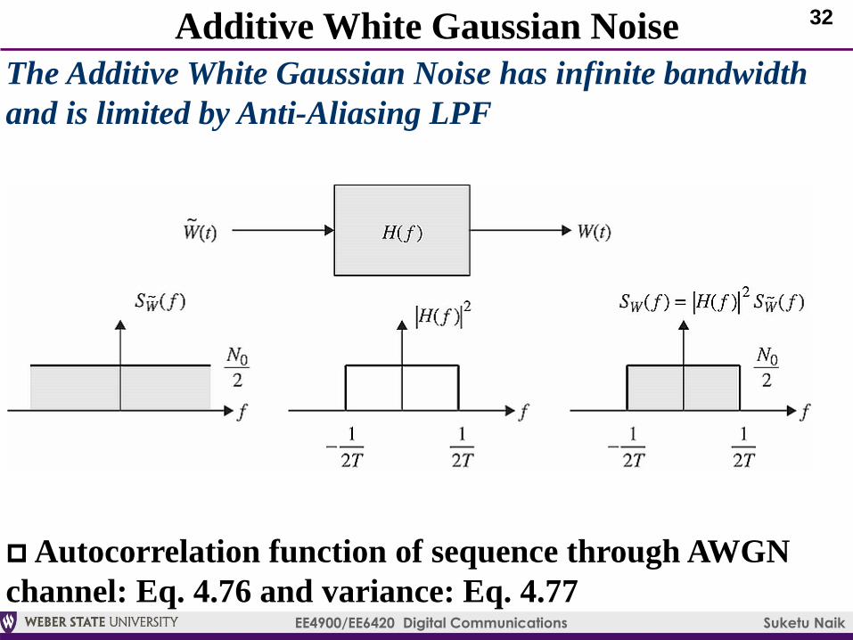
Additive White Gaussian Noise
The Additive White Gaussian Noise has infinite bandwidth
and is limited by Anti-Aliasing LPF
Autocorrelation function of sequence through AWGN
channel: Eq. 4.76 and variance: Eq. 4.77


