
9/21/2019
1
Electromagnetics:
Electromagnetic Field Theory
Transmission Line Equations
Lecture Outline
• Introduction• Transmission Line Equations
• Transmission Line Wave Equations
Slide 2
1
2
9/21/2019
2
Slide 3
Introduction
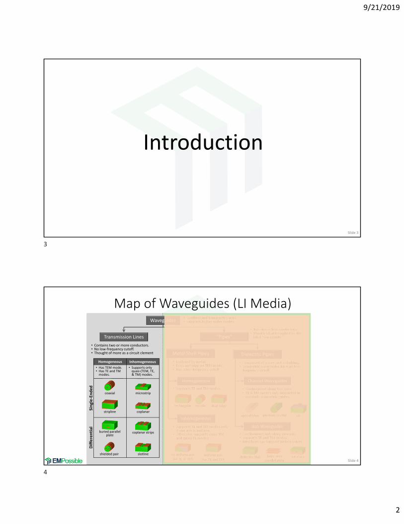
Map of Waveguides (LI Media)
Slide 4
Transmission Lines
• Contains two or more conductors.• No low‐frequency cutoff.• Thought of more as a circuit clement
• Confines and transports waves.• Supports higher‐order modes.
• Has TEM mode.• Has TE and TM modes.
stripline
coaxial microstrip
slotline
coplanar
“Pipes”
• Has one or less conductors.• Usually what is implied by the label “waveguide.”
Metal Shell Pipes Dielectric Pipes
Inhomogeneous
Homogeneous
• Enclosed by metal.• Does not support TEM mode.• Has a low frequency cutoff.
• Supports TE and TM modes
• Supports TE and TM modes only if one axis is uniform.
• Otherwise supports quasi‐TM and quasi‐TE modes.
rectangular circular
Channel Waveguides
Slab Waveguides
• Composed of a core and a cladding.• Symmetric waveguides have no low‐frequency cutoff.
• Confinement only along one axis.• Supports TE and TM modes.• Interfaces can support surface waves.
• Confinement along two axes.• TE & TM modes only supported in circularly symmetric guides.
dielectric Slab interface
optical Fiber rib
dual‐ridge
no uniform axis(no TE or TM)
Waveguides
Homogeneous Inhomogeneous
• Supports only quasi‐(TEM, TE, & TM) modes.
Single‐Ended
Differential
buried parallel plate
coplanar strips
photonic crystal
shielded pairlarge‐area
parallel plate
uniform axis(has TE and TM)
3
4

9/21/2019
3
Signals in Transmission Lines: Coax
Slide 5
Signals in Transmission Lines: Microstrip
Slide 6
5
6
9/21/2019
4
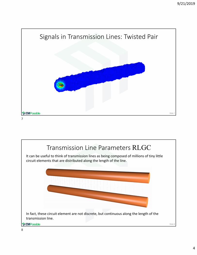
Signals in Transmission Lines: Twisted Pair
Slide 7
Transmission Line Parameters RLGC
Slide 8
It can be useful to think of transmission lines as being composed of millions of tiny little circuit elements that are distributed along the length of the line.
In fact, these circuit element are not discrete, but continuous along the length of the transmission line.
7
8
9/21/2019
5
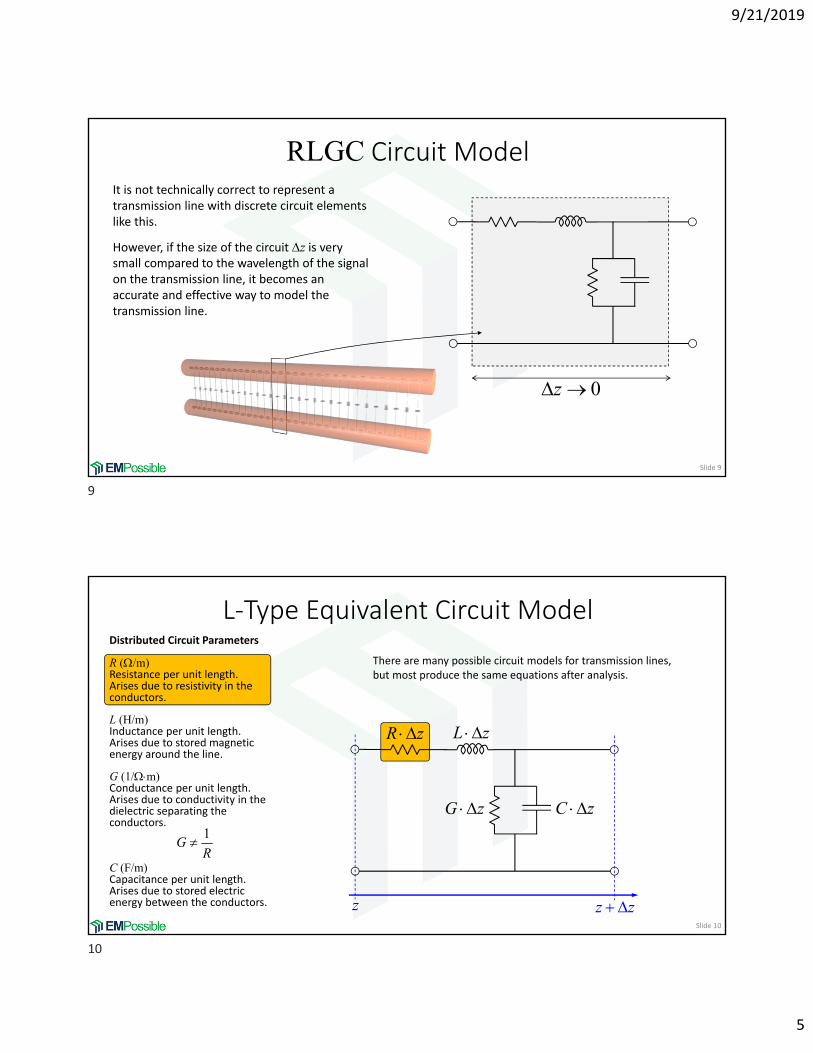
RLGC Circuit Model
Slide 9
It is not technically correct to represent a transmission line with discrete circuit elements like this.
However, if the size of the circuit z is very small compared to the wavelength of the signal on the transmission line, it becomes an accurate and effective way to model the transmission line.
0z
L‐Type Equivalent Circuit Model
Slide 10
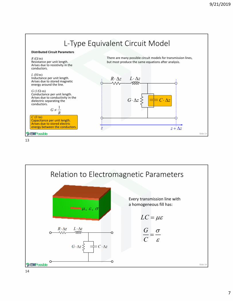
Distributed Circuit Parameters
R (/m)Resistance per unit length. Arises due to resistivity in the conductors.
L (H/m)Inductance per unit length. Arises due to stored magnetic energy around the line.
G (1/m)Conductance per unit length. Arises due to conductivity in the dielectric separating the conductors.
C (F/m)Capacitance per unit length. Arises due to stored electric energy between the conductors. z z z
R z L z
G z C z
There are many possible circuit models for transmission lines, but most produce the same equations after analysis.
1G
R
9
10

9/21/2019
6
L‐Type Equivalent Circuit Model
Slide 11
Distributed Circuit Parameters
R (/m)Resistance per unit length. Arises due to resistivity in the conductors.
L (H/m)Inductance per unit length. Arises due to stored magnetic energy around the line.
G (1/m)Conductance per unit length. Arises due to conductivity in the dielectric separating the conductors.
C (F/m)Capacitance per unit length. Arises due to stored electric energy between the conductors. z z z
R z L z
G z C z
There are many possible circuit models for transmission lines, but most produce the same equations after analysis.
1G
R
L‐Type Equivalent Circuit Model
Slide 12
Distributed Circuit Parameters
R (/m)Resistance per unit length. Arises due to resistivity in the conductors.
L (H/m)Inductance per unit length. Arises due to stored magnetic energy around the line.
G (1/m)Conductance per unit length. Arises due to conductivity in the dielectric separating the conductors.
C (F/m)Capacitance per unit length. Arises due to stored electric energy between the conductors. z z z
R z L z
G z C z
There are many possible circuit models for transmission lines, but most produce the same equations after analysis.
1G
R
11
12
9/21/2019
7
L‐Type Equivalent Circuit Model
Slide 13
Distributed Circuit Parameters
R (/m)Resistance per unit length. Arises due to resistivity in the conductors.
L (H/m)Inductance per unit length. Arises due to stored magnetic energy around the line.
G (1/m)Conductance per unit length. Arises due to conductivity in the dielectric separating the conductors.
C (F/m)Capacitance per unit length. Arises due to stored electric energy between the conductors. z z z
R z L z
G z C z
There are many possible circuit models for transmission lines, but most produce the same equations after analysis.
1G
R
Relation to Electromagnetic Parameters
Slide 14
LC , ,
G
C
Every transmission line with a homogeneous fill has:
13
14
9/21/2019
8
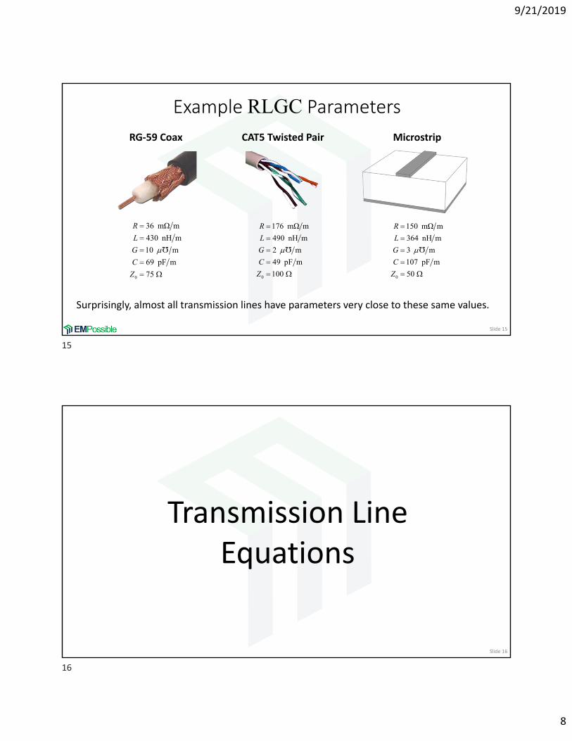
Example RLGC Parameters
Slide 15
0
36 mΩ m
430 nH m
10 m
69 pF m
75
R
L
G
C
Z
0
176 mΩ m
490 nH m
2 m
49 pF m
100
R
L
G
C
Z
Surprisingly, almost all transmission lines have parameters very close to these same values.
0
150 mΩ m
364 nH m
3 m
107 pF m
50
R
L
G
C
Z
RG‐59 Coax CAT5 Twisted Pair Microstrip
Slide 16
Transmission Line Equations
15
16
9/21/2019
9
E & H V and I
Slide 17
Fundamentally, all circuit problems are electromagnetic problems and can be solved as such.
All two‐conductor transmission lines either support a TEM wave or a wave very closely approximated as TEM.
An important property of TEM waves is that E is uniquely related to V and H and uniquely related to E.
L
V E d
L
I H d
This reduces analysis of transmission lines to just V and I. This makes analysis much simpler because these are scalar quantities!
Transmission Line Equations
Slide 18
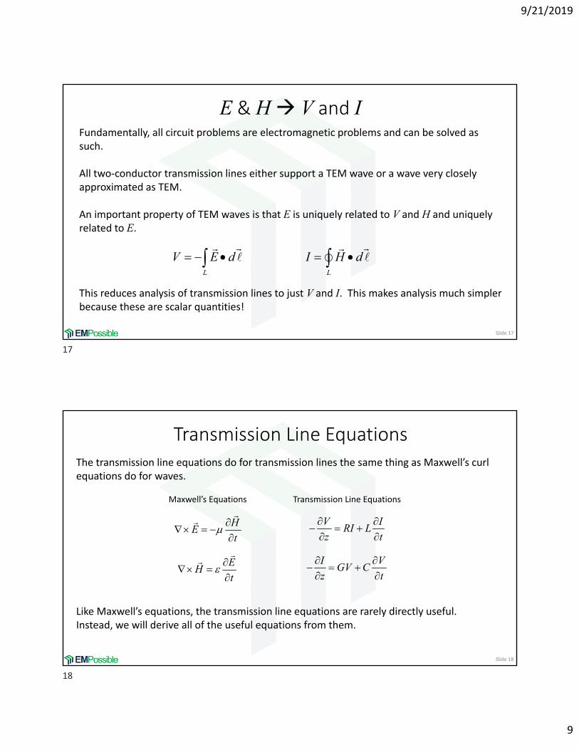
The transmission line equations do for transmission lines the same thing as Maxwell’s curl equations do for waves.
Maxwell’s Equations Transmission Line Equations
HE
t
EH
t
V IRI L
z t
I VGV C
z t
Like Maxwell’s equations, the transmission line equations are rarely directly useful. Instead, we will derive all of the useful equations from them.
17
18

9/21/2019
10
,V z t ,I z t
L zt
,I z t R z ,V z z t
Derivation of First TL Equation (1 of 2)
Slide 19
z z z
R z L z
G z C z
+
‐
,V z t
+
‐
,V z z t
Apply Kirchoff’s voltage law (KVL) to the outer loop of the equivalent circuit:
1
2 3
4
,I z t
1 23
4
0
Derivation of First TL Equation (2 of 2)
Slide 20
We rearrange the equation by bringing all of the voltage terms to the left‐hand side of the equation, bringing all of the current terms to the right‐hand side of the equation, and then dividing both sides by z.
,, , , 0
, , ,,
I z tV z t I z t R z L z V z z t
t
V z z t V z t I z tRI z t L
z t
In the limit as z 0, the expression on the left‐hand side becomes a derivative with respect to z.
, ,,
V z t I z tRI z t L
z t
19
20

9/21/2019
11
,0
V z z tC z
t
,G zV z z t ,I z z t
Derivation of Second TL Equation (1 of 2)
Slide 21
z z z
R z L z
G z C z
+
‐
,V z t
+
‐
,V z z t
1 2
3 4
Apply Kirchoff’s current law (KCL) to the main node the equivalent circuit:
,I z t
,I z t
1 2 34
,I z z t
Derivation of Second TL Equation (2 of 2)
Slide 22
We rearrange the equation by bringing all of the current terms to the left‐hand side of the equation, bringing all of the voltage terms to the right‐hand side of the equation, and then dividing both sides by z.
,, , , 0
, , ,,
V z z tI z t I z z t G zV z z t C z
t
I z z t I z t V z z tGV z z t C
z t
In the limit as z 0, the expression on the left‐hand side becomes a derivative with respect to z.
, ,,
I z t V z tGV z t C
z t
21
22

9/21/2019
12
Slide 23
Transmission Line Wave Equations
Starting Point – Telegrapher Equations
Slide 24
Start with the transmission line equations derived in the previous section.
, ,,
V z t I z tRI z t L
z t
, ,
,I z t V z t
GV z t Cz t
time‐domain
For time‐harmonic (i.e. frequency‐domain) analysis, Fourier transform the equations above.
dV zR j L I z
dz
dI zG j C V z
dz frequency‐domain
Note: The derivative d/dz became an ordinary derivative because z is the only independent variable left.
These last equations are commonly referred to as the telegrapher equations.
23
24

9/21/2019
13
Wave Equation in Terms of V(z)
Slide 25
To derive a wave equation in terms of V(z), first differentiate Eq. (1) with respect to z.
dV zR j L I z
dz
dI zG j C V z
dz Eq. (1) Eq. (2)
2
2
d V z dI zR j L
dz dz Eq. (3)
Second, substitute Eq. (2) into the right‐hand side of Eq. (3) to eliminate I(z) from the equation.
2
2
d V zR j L G j C V z
dz
Last, rearrange the terms to arrive at the final form of the wave equation.
2
20
d V zR j L G j C V z
dz
Wave Equation in Terms of I(z)
Slide 26
To derive a wave equation in terms of I(z), first differentiate Eq. (2) with respect to z.
dV zR j L I z
dz
dI zG j C V z
dz Eq. (1) Eq. (2)
2
2
d I z dV zG j C
dz dz Eq. (3)
Second, substitute Eq. (1) into the right‐hand side of Eq. (3) to eliminate V(z).
2
2
d I zG j C R j L I z
dz
Last, rearrange the terms to arrive at the final form of the wave equation.
2
20
d I zG j C R j L I z
dz
25
26
9/21/2019
14
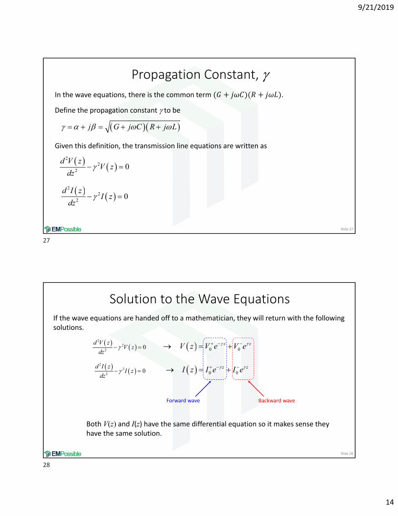
Propagation Constant,
Slide 27
Define the propagation constant to be
j G j C R j L
Given this definition, the transmission line equations are written as
2
22
0d V z
V zdz
2
22
0d I z
I zdz
In the wave equations, there is the common term 𝐺 𝑗𝜔𝐶 𝑅 𝑗𝜔𝐿 .
Solution to the Wave Equations
Slide 28
If the wave equations are handed off to a mathematician, they will return with the following solutions.
2
22
0d V z
V zdz
2
22
0d I z
I zdz
0 0 z zV z V e V e
0 0 z zI z I e I e
Both V(z) and I(z) have the same differential equation so it makes sense they have the same solution.
Forward wave Backward wave
27
28


