LED Induced Fluorescence using microscale visualization
methods
Jorge André Garcia Arromba
Thesis to obtain the Master of Science Degree in
Mechanical Engineering
Supervisor: Prof. António Luís Nobre Moreira
Examination Committee
Chairperson: Prof. Viriato Sérgio de Almeida Semião
Supervisor: Prof. António Luís Nobre Moreira
Member of the Committee: Prof. José Maria Campos da Silva André
October 2014

i

ii
Acknowledgements
First of all, I would like to thank my supervisor Professor Luís Moreira for the opportunity of working
with him and his availability, patience and guidance throughout the elaboration of this work.
Financial support through project PTDC/EME-MFE/109933/2009 from Fundação para a Ciência e a
Tecnologia, FCT, is gratefully acknowledged. Laboratory facilities were built in the framework of project
RECI/EMS-SIS/0147/2012 and therefore also acknowledged.
I would like to express my gratitude towards Vânia Silvério, for all the help, discussions, guidance,
lectures and laughs. Your support was essential for the outcome of this work, and thank you for
believing in me and for the encouragement until the very end.
To all my closest friends, and to my fellow colleagues in the Laboratory, for the support, fellowship and
understanding that helped me to go through this 6 months and take this to a conclusion, thank you.
At last, but not at least, I thank all the unconditional love and support from my family. To my brother,
my parents, I am infinitely grateful to you. Love you all.

iii
iv
Resumo
Este trabalho consiste na optimização e aplicação de duas técnicas de fluorescência, utilizando um ou
dois corantes, para medição não intrusiva da temperatura em escoamento à microescala. Foram
efetuadas medições num sistema microfluídico, iluminado em volume com uma fonte de luz LED, a
partir das quais se definiram e otimizaram os parâmetros que determinam a precisão do método.
Posteriormente a técnica foi aplicada a dois casos de teste, ao escoamento num microcanal de
paredes aquecidas e a uma mistura térmica de dois escoamentos numa zona de mistura em T.
Foram utilizados dois corantes, Rodamina B e Rodamina 110, uma vez que a intensidade de
fluorescência emitida por cada um deles varia de forma diferente com a temperatura. Enquanto o sinal
da Rodamina B apresenta uma dependência acentuada da temperatura, o da Rodamina 110 é
aproximadamente independente (sensibilidade < 0.011 %. ℃−1). A técnica de um corante (RhB)
apresentou-se mais vantajosa, com sensibilidade de 1.68 %. ℃−1, sendo posteriormente aplicada ao
caso prático num microcanal, onde foi encontrada concordância na variação de temperatura medida
através de um termopar na sua parede. Os erros associados à medição do sinal de intensidade de
fluorescência são inferiores a 3.8% enquanto os associados às medidas de temperatura são inferiores a
0.71%.
Medidas das distribuições bidimensionais de temperatura no escoamento de soluções aquosas de
corantes com corantes em concentrações residuais num canal de dimensões micrométricas
comprovaram a capacidade da técnica ser aplicada com a fonte de iluminação LED e com elevadas
resoluções espacial (1.54 𝜇𝑚) e temporal (~5 𝑚𝑠).
Palavras-chave: Técnica de Fluorescência, Iluminação LED, Medição temperatura escoamento,
Microfluidos, Perfis de temperatura 2D.

v
Abstract
A non-intrusive LED Induced Fluorescence Thermometry measurement technique is developed and
applied using microscale visualization techniques. Whole field temperature measurements in a
volume-illuminated microfluidic setup were performed with a good spatial and temporal resolutions,
being applied to practical that serve as training benchmark tests, often imposed to CPU chips, and to
the thermal mixing of two fluid streams in a T-shaped micro-mixer.
Two different techniques are addressed: Normalized Induced Fluorescence Thermometry (N-LED-IFT)
and Normalized Ratiometric Induced Fluorescence Thermometry (NR-LED-IFT), using one and two
dyes, respectively. Parameters influencing the results and the feasibility of these techniques at the
microscale using a Leica illumination system LED SFL100 530 𝑛𝑚 were also addressed.
Rhodamine B and Rhodamine 110 are used as temperature sensitive and insensitive dyes, respectively.
The single-dye technique (N-LED-IFT) proved most advantageous, obtaining a sensitivity of
1.68 %. ℃−1. This technique was then used for training benchmark testing, where good agreement with
temperature variations on wall temperature measured using a thermocouple was found. The N-LED-IFT
results present errors lower than 3.8 % in fluorescence intensity and lower than 0.71 % in temperature
measurements. Radial and longitudinal temperature profiles in the microchannel were also observed.
The capability of this technique to be applied to low and high velocity microscale flows using a LED
illumination source was proved and 2D fluid temperature profiles where obtained with high spatial
(1.54 𝑚) and temporal (~ 5 𝑚𝑠) resolutions.
Keywords: LED Induced Fluorescence Thermometry, LED illumination, Flow temperature measurement,
Microfluidics, 2D fluid temperature profiles.

vi
Nomenclature
𝐴 – Cross section area [𝑚2]
𝐴1→2 – External area between sections 1 and 2
[𝑚2]
𝑏 – Number of bits
C – Dye concentration in the solution [𝑘𝑔/𝑚3]
𝐶𝑝 – Specific heat of the fluid [𝐽. 𝑘𝑔−1. 𝐾−1]
𝐷ℎ – Hydraulic diameter [𝑚]
𝐹 – Light fraction [−]
ℎ – Heat transfer coefficient [𝑊. 𝐾−1. 𝑚−2]
𝐼 – Fluorescent intensity emitted per unit of
volume [𝐴. 𝑈. ]
𝐼0 – Light incident flux [𝑊/𝑚2]
𝐿 – Percentage of energy loss from the
resistance directly to environment [−]
𝐿𝐻𝑒 – Hydrodynamic entrance length [𝑚]
𝐿𝑇𝑒 – Thermal entrance length [𝑚]
�̇� – Mass flow [𝑘𝑔. 𝑠−1]
𝑝 – Perimeter [𝑚]
𝑃 – Output electrical power from power
generator [𝑊]
Particles A – Temperature dependent dye
particles
Particles B – Temperature independent dye
particles
𝑃𝑟 – Prandtl number [−]
𝑄 – Volumetric flow [𝑚𝑙. ℎ−1]
𝑞′′ – Heat flux [𝑊. 𝑚−2]
𝑞1→2′′ – Net heat flux dissipated from section 1
to section 2 [𝑊. 𝑚−2]
𝑅𝑒 – Reynolds number [−]
SNR – Signal-to-Noise Ratio [dB]
𝑇 – Temperature [𝐾 𝑜𝑟 ℃]
𝑈 – Flow velocity, eq. 22 and 23 [𝑚. 𝑠−1]
𝑈 – Voltage [𝑉]
𝑉 – Signal output from camera [𝑉]
𝑉 – Solution volume, Equation 24 [𝑚3]
Greek symbols
βC – Collection efficiency
∆𝑇 – Temperature difference [𝐾 𝑜𝑟 ℃]
휀 – Absorption coefficient [𝑚2/𝑘𝑔]
𝛬 – Microchannel characteristic dimension [𝑚]
𝜆0 – Wavelength of light in vacuum [𝑚]
𝜇 – Mean intensity of the image set [𝐴. 𝑈. ]
𝜐 – Fluid kinematic velocity [𝑚2. 𝑠−1]
𝜌 – Fluid density [𝑘𝑔. 𝑚−3]
𝜎 – Standard deviation of the image set,
Equation 16 [𝐴. 𝑈. ]
𝛷 – Quantum yield [−]

vii
Acronyms
CCD – Charge Coupled Device
CPU – Central Processing Unit
DOF – Depth Of Field
FRET – Fluorescent Resonance Energy Transfer
FS – Fluorescence Signal
IC – Integrated Circuits
LaVision HSS – LaVision HighSpeedStar high
speed imaging camera
LED – Light emitting diode
LED-IFT – LED Induced Fluorescence
Thermometry
LIF – Laser Induced Fluorescence
NA – Numerical Aperture
N-LIFT – Normalized Laser Induced
Fluorescence Thermometry
N-LED-IFT – Normalized LED Induced
Fluorescence Thermometry
NR-LIFT – Normalized Ratiometric Laser
Induced Fluorescence Thermometry
NR-LED-IFT – Normalized Ratiometric LED
Induced Fluorescence Thermometry
Phantom – Vision Research Phantom v4.0 high
speed imaging camera
RhB – Rhodamine B, temperature dependent
dye
Rh110 – Rhodamine 110, temperature
independent dye
TLCs – Thermochromic Liquid Crystals
VLSI – Very Large Scale Integration systems
Subscripts
𝐴 – Related to Particles A
𝐵 – Related to Particles B
𝑖 – Inner dimension
𝑜 – Outer dimension
Superscripts
𝛼 – Image that captures particles A
fluorescence emission
𝛽 – Image that captures particles B
fluorescence emission

viii
Table of Contents
Acknowledgements ....................................................................................................................................................................... ii
Resumo ............................................................................................................................................................................................. iv
Abstract .............................................................................................................................................................................................. v
Nomenclature ................................................................................................................................................................................. vi
List of Tables ................................................................................................................................................................................... ix
List of Figures .................................................................................................................................................................................. x
1. Introduction ................................................................................................................................................................................. 1
2. Objectives and Dissertation Outline .................................................................................................................................. 4
3. Principles of the LIF for thermometry measurements ................................................................................................ 5
4. Experimental Campaign....................................................................................................................................................... 13
4.1 Flow Configurations ....................................................................................................................................................... 13
Microchannel flow ............................................................................................................................................................. 13
T-shaped micro-mixer ..................................................................................................................................................... 18
4.2 Equipment .......................................................................................................................................................................... 20
Microscope ........................................................................................................................................................................... 20
High speed cameras ......................................................................................................................................................... 21
Illumination system ........................................................................................................................................................... 25
Pumping systems ............................................................................................................................................................... 26
4.3 Experimental method .................................................................................................................................................... 27
Fluorescent dyes ................................................................................................................................................................ 27
Calibration of the fluorescence intensity.................................................................................................................. 29
Uncertainty estimates ...................................................................................................................................................... 31
5. Results and Discussion ......................................................................................................................................................... 32
5.1. Test Parameters .............................................................................................................................................................. 32
Dye Concentration ............................................................................................................................................................ 34
Influence of Background Noise .................................................................................................................................... 35
Auto-absorption and Beer-Lambert Law ................................................................................................................. 37
Calibration Curves – NR-LED-IFT vs N-LED-IFT ..................................................................................................... 38
N-LED-IFT .............................................................................................................................................................................. 39
5.2. Application of the LED-IFT technique .................................................................................................................... 42
Training Benchmark .......................................................................................................................................................... 42
T-shaped micro-mixer ..................................................................................................................................................... 45
6. Concluding Remarks and Future Work ......................................................................................................................... 47
References...................................................................................................................................................................................... 49
Appendix ........................................................................................................................................................................................ 52
Processing algorithm ............................................................................................................................................................ 52

ix
List of Tables
Table 1 – Glass microchannel installation characteristics. .......................................................................................... 15
Table 2 – Main characteristics of the high speed cameras used. ............................................................................. 24
Table 3 – Correspondence between the pixel and image size and depth of field in both high speed
cameras for different optical arrangements. .................................................................................................................... 25
Table 4 – Characteristics of aqueous solutions of Rhodamine B and Rhodamine 110 in de-ionized water
at 20 ℃ ............................................................................................................................................................................................ 27
Table 5 – Aqueous solutions used in experiments. ....................................................................................................... 28
x
List of Figures
Figure 1 – Example of Perrin-Jablonski Diagram with absorption and radiative dissipation methods
examples. S0, S1 and S2 – singlet electronic states; T1, T2 – triplet electronic states; IC – internal
conversion; ISC – intersystem crossing (adapted from [35]). ....................................................................................... 6
Figure 2 – Schematics of the microchannel experimental setup. ............................................................................ 14
Figure 3 – Detail of thermocouples location in the microchannel experimental setup. ................................. 15
Figure 4 – Example of temperature response after an imposed heat flux increase. ........................................ 17
Figure 5 – Schematics of the T-shaped micro-mixer experimental setup. ........................................................... 18
Figure 6 – T-shaped micro-mixer scheme. ....................................................................................................................... 19
Figure 7 – Secondary flow loop used to control the temperature of the hot flow. Reservoir,
potentiometer and two electric resistances. .................................................................................................................... 19
Figure 8 – Leica DM IL inverted microscope. Image extracted from [43]. ............................................................ 20
Figure 9 – LaVision HighSpeedStar high speed camera with the x0.55 CCD adapter. ..................................... 21
Figure 10 – Phantom v4.2 high speed camera and custom made support attached to the inverted
microscope. ................................................................................................................................................................................... 22
Figure 11 – Rhodamine B filter characteristics. Transmission percentage as function of wavelength.
(Chroma Technology Corp., Scan range from 480.0 𝑛𝑚 to 680 𝑛𝑚, ET-TRITC Filter Set for 530 LED_Leica
DMR_Un-Mounted). .................................................................................................................................................................... 23
Figure 12 – Rhodamine 110 filter characteristics: Transmission percentage as function of wavelength.
(Melles Griot 03FIL004 Laser Filter 514.5 𝑛𝑚 25 DIA, 03FIL00405100762). .......................................................... 23
Figure 13 – HighSpeedStar calibration target from LaVision represented in a) and in b) the reticle from
Peak Optics used to establish the correspondence of pixel to image size for both cameras...................... 24
Figure 14 – Leica LED SFL100 illumination system. ....................................................................................................... 26
Figure 15 – Pumping systems: a) NE-300 syringe pump and b) Harvard 22 syringe pump. ........................ 26
Figure 16 – Visual aspect of three solutions used. From left to right: RhB with a concentration of 20
mg.L-1; RhB with a concentration of 20 mg.L-1 and Rh110 with a concentration of 15 mg.L-1; Rh110 with
a concentration of 50 mg.L-1. ...................................................................................................................................... 28
Figure 17 – Schematics of the thermally insulated pool. ............................................................................................ 29
Figure 18 – Schematics of the calibration setup............................................................................................................. 30
Figure 19 – Fluorescent intensity signal of a) RhB collected with HighSpeedStar high speed
visualization camera and b) Rh110 collected with Phantom V4.2 high speed visualization camera in
microchannel experiments ...................................................................................................................................................... 32
Figure 20 – MATLAB® equivalent images to those of Figure 18: a) RhB and b) Rh110. ................................. 33
Figure 21 – Fluorescence intensity response obtained for the same control point for seven aqueous
RhB solutions with different concentrations. ................................................................................................................... 34
Figure 22 – Influence of solution concentration in fluorescence signal sensitivity. ......................................... 35
Figure 23 – Fluorescent signal from both dyes, for the same control point, with and without room
illumination. ................................................................................................................................................................................... 36
Figure 24 – Rhodamine B fluorescent signal with and without background image removal. ..................... 36
Figure 25 – Fluorescent signal on HSS image for both particles, separately and with both in solution. . 37
Figure 26 – RhB and Rh110 fluorescence signal (FS) response to temperature. ............................................... 38

xi
Figure 27 – LED-IFT techniques comparison: NR-LED-IFT in solid squares and N-LED-IFT in hollow
triangles. ......................................................................................................................................................................................... 39
Figure 28 – RhB fluorescence signal collected in the Pool Calibration system. ................................................. 40
Figure 29 – Normalized intensity for 6 different control points............................................................................... 41
Figure 30 – Calibration curve for the N-LED-IFT technique with a 4th order best fit polynomial. .............. 41
Figure 31 – Microchannel setup. ........................................................................................................................................... 43
Figure 32 – Flow temperature represented in purple, wall temperature in blue and power output from
power source in black. .............................................................................................................................................................. 44
Figure 33 – Detail on the responses from the N-LED-IFT technique and from the thermocouple
measurements for a power increase. .................................................................................................................................. 45
Figure 34 – Mixing plane of two laminar stream flows with different velocities: a) 𝑄𝑐𝑜𝑙𝑑 = 200 𝑚𝑙. ℎ − 1,
𝑄ℎ𝑜𝑡 = 200 𝑚𝑙. ℎ − 1; b) 𝑄𝑐𝑜𝑙𝑑 = 300 𝑚𝑙. ℎ − 1, 𝑄ℎ𝑜𝑡 = 300 𝑚𝑙. ℎ − 1; c) 𝑄𝑐𝑜𝑙𝑑 = 500 𝑚𝑙. ℎ − 1,
𝑄ℎ𝑜𝑡 = 50 𝑚𝑙. ℎ − 1. Cold fluid coming from left to right and hot fluid inlet is on the top. ........................ 46
Figure 35 – Mixing plane of two stream flows for the same volumetric flow, 𝑄𝑐𝑜𝑙𝑑 = 1000 𝑚𝑙. ℎ −
1 and 𝑄ℎ𝑜𝑡 = 1000 𝑚𝑙. ℎ − 1. Consecutive images captured with a 200 𝐻𝑧 acquisition rate. Cold fluid
coming from the left to the right and hot fluid inlet on the top. ............................................................................ 46

1
1. Introduction
Faster and smaller electronic parts are consistently being developed at the same time the number of
transistors per chip is increasing and consequently the heat flux dissipated, which can exceed
100 W.cm-2. In order to remove such high heat rates, air cooling or single-phase liquid cooling in plain
channels in contact with the chip are becoming insufficient [1]. The need to explore the use of
microchannel heat sinks to achieve high cooling rates emerged, and Tuckerman & Pease in 1981 [2]
developed and tested the first VLSI system. After that, a large number of researchers have addressed
the microscale heat transfer issues. Comprehensive literature reviews on the fluid flow, transport and
heat transfer in microchannel heat sinks for both, single and two-phase regimes can be found in [3, 4].
However, measurements of the temperature distribution in microscale flow systems still represents one
of the most challenging aspects of experimentation due to very small temperature gradients
associated with the high heat transfer rates and short heat dissipation timescales [5].
In line with this, temperature measurements in microscale field of research gained some highlight and
preponderance due to the lack of knowledge and the need to control small scale transport and heat
transfer phenomena in different areas of interest, such as biochemistry [6] and electronics [7, 8].
Widely-used methods for measurement of fluid temperature at macroscale cannot be directly applied
to the microscale. Well known contacting measurement devices like high-precision thermocouple
probes are not the ideal solution [9]. Besides being intrusive, these probes have poor spatial and
temporal resolution since most of them have a characteristic size comparable to the cross section of
the microchannels. Embedded thermocouples along the microchannel base [10] or inside its walls [11,
12] have also been used, however the spatial resolution remains low.
Microfluidic devices fabricated with integrated resistance temperature detectors (RTDs) are a viable
alternative, which allows surface temperature monitoring and, although presenting a better spatial
resolution, do not provide information on the local fluid temperature [13]. Infrared thermography can
also be used but is limited to its sole application in surfaces, requiring an accurate value of the
emissivity of the medium [14, 15] and, thus, increasing its complexity. On the other hand,
thermochromic liquid crystals (TLCs) [16] can be used in solution to measure fluid flow temperature
with a maximum spatial resolution of approximately 1 m, while encapsulated TLCs can vary from 10
to 150 𝑚 [9]. However, limitations associated with the range of temperature still exist, from ~1 ℃ for
narrow-band TLCs and from 5 to 20 ℃ for wide-band TLCs [17]. For example, Richards et al. in 1998
[18] measured temperatures between 30 and 35 ℃ with a temporal resolution of 30 𝜇𝑠 and a spatial

2
resolution of 100 𝑚, and in the work of Lin and Kandlikar [19] stainless steel microtubes were used
addressing temperature variations from 35 to 45 ℃ and from 42 to 47 ℃.
But in experimental microfluidics, optical measurement techniques acquired increased relevance in the
last decade (due to progresses in IC technology), allowing higher resolutions and acquisition frame
rates. Software for image processing has also been improved. In this context, Laser Induced
Fluorescence Thermometry (LIFT) emerged, among other options, as a non-intrusive technique able to
make whole-field temperature measurements inside a volume of fluid by capturing the fluorescence
light emitted by particles in solution and making use of high spatial and temporal resolution
illumination and recording systems.
The LIFT technique has been first used by Omenetto et al. in 1972 [20] to measure the temperature of
reacting species or dyes in flames, followed by and Chan & Daily in 1980 [21] in the same research
area. The technique then evolved capitalizing on fluorescent dye properties: when excited at certain
wavelengths by an illumination source, the dyes emit a fluorescent light in a different wavelength
band, higher than the excitation one.
In the early stages of the Laser Induced Fluorescence, mostly in macroscale flows (late 90’s), a
temperature dependent dye was dissolved in the flowing fluid in order to apply the technique [22–24].
Detailed studies on different fluorescent dyes and their compatibility can be found in [25, 26].
However, the quality of such measurements is still hindered by the difficulties in guaranteeing a
homogeneous illumination intensity distribution and recording imperfections. A new two-color LIFT
technique was then proposed by Sakakibara & Adrian in 1999 [27], who added a temperature-
insensitive dye to be used as a reference to compensate for the fluctuations at illumination.
Experiments performed in 2004 by Lavieille et al. [28] on heated jets showed that the droplet size
influences the results from the two-dye technique. The authors suggested a new approach that
consists in considering the ratio of fluorescence light emitted by the temperature-dependent dye at
different spectral frequencies, also called the single dye, two color LIFT method. Bruchhausen et al. in
2004 [29] were the first to apply the single dye, two color LIFT using a pulsed Nd:YAG laser, achieving
shorter timescales than those from thermal transport at the microscale.
The first temperature measurements via volume illumination in microscale were reported by Ross et al.
in 2001 [30] with a claimed accuracy of ±1.5 ℃. A standard fluorescence microscope and a CCD
camera were used to measure the temperature distribution in the flow inside microchannels, with
spatial and temporal resolutions of 1 𝜇𝑚 and 33 ms, respectively. Yoon & Kim in 2006 [31] introduced
an ultra-thin laser sheet (10 µm thickness) as an illumination source in microchannel experiments but

3
their results accuracy could not be retrieved since no temperature measurements were performed;
only measurements of concentration distribution of the suspended particles were made. Natrajan and
Christensen [5] highlighted, in 2008, the importance of the illumination intensity and the need to
illuminate over timescales much shorter than those of the microscale thermal transport. In this context,
the authors used a pulsed Nd:YAG laser and applied the two-color LIFT technique achieving
uncertainties of ±0.55 ℃ and ±0.45 ℃ for dyes diluted in ethanol and water, respectively. Chamarty et
al. in 2010 [9] designed a setup to perform experiments using two fluorescent dyes. A single camera
captured two sequential images (each image corresponding to the signal emitted by each dye in
solution) by using a filter wheel with two filters, one for each dye, acknowledging the fact that this
setup could only be appropriate to study steady flows as there is necessarily a time delay between the
first and second images. Uncertainties of ±1.25 ℃ and of ±2.68 ℃ were found for traditional single-
dye and two-dye LIFT, respectively. Sakakibara & Adrian in 2004 [32] claimed an uncertainty of ±0.2 ℃
using the two-dye LIFT. Better results were attributed to the use of a 14-bit digital CCD camera and by
using a new convolution technique that allowed them to remove more efficiently some blurring
present on fluorescent images.
Moreover, the standard light source of LIF used at macroscale is a continuous, usually Argon laser,
which does not provide sufficient illumination intensity over the much shorter thermal transport at the
microscale and, therefore, does not allow obtaining accurate instantaneous measurements of
temperature. Pulsed lasers, such as the Nd:YAG laser, can provide higher peak power than the
continuous-wave lasers at the same time that the short pulse time is useful for good temporal
resolution [5]. More recently, laser diodes emitting in the ultraviolet region of the spectrum provided
compact solutions for fluorescence emission from blue to near-infrared [33]. However, though
compact, they can provide low output power and are expensive. Recently, high-power LEDs emitting in
the ultraviolet became commercially available and, though both LED and laser diodes (LDs) are small in
size, LEDs have longer operating lifetimes, are stable, have reasonable input power requirements and
are of low cost and accessible [34]. The use of LEDs, emitting in the visible region, are then considered
as a viable and more affordable alternative light source.
Fluorescence techniques have been applied for more than 20 years, being fluid temperature
measurements essential to enhance heat transfer phenomena studies. Going from the utilization of
one, in its early stages, to the usage of three fluorescent dyes more recently, the normalized
techniques using one or two fluorescent dyes are assessed in the present study to measure fluid
temperature at microscale as well as the usage of a fluorescent LED, as an alternative illumination
source to traditional lasers.
4
2. Objectives and Dissertation Outline
Temperature measurements are essential to study heat transport phenomenon, which is the major
field of research in the Multiscale Transport Phenomena Laboratory, part of the Centre for Innovation,
Technology and Policy Research, IN+, at the Mechanical Engineering Department of Instituto Superior
Técnico. To complement ongoing research, LED-IFT, a non-intrusive technique that can be applied to
microfluids is implemented, allowing whole field temperature measurements in a volume-illuminated
microfluidic setup with good spatial and temporal resolutions.
In this context, and in the wake of the conclusions of the literature review in chapter 1, the present
thesis considers the implementation and experimental characterization of a Light Induced
Fluorescence Thermometry technique at microscale. In particular, the study assesses the feasibility of
applying the two-dye LED-IFT approach at the microscale using a Leica illumination system LED SFL100
530 𝑛𝑚. The development of image processing algorithms along with the experimental setup
idealization and concretization are essential parts of this thesis.
As in previous researches, both at micro and macroscale, this study considers the use of Rhodamine B
and Rhodamine 110 as the temperature sensitive and insensitive dyes, respectively. The performance
of this two-dye approach (NR-LED-IFT) for microfluidic temperature measurement is compared with
that of the single-dye approach (N-LED-IFT). The most adequate is then tested in two practical
examples: a training benchmark test applied to a microchannel with heated walls, often used for CPU
chips, and visualization of the thermal mixing of two flows in a T-shaped micromixer. These tests allow
to evaluate quantitatively the results and the spatial and temporal resolutions of the technique, along
with its application to some fields of research where this technique can be crucial for scientific
enhancements, such as in heat transfer experiments with different flow regimes turbulent performed at
microscale.

5
3. Principles of the LIF for thermometry measurements
Laser or LED Induced Fluorescence Thermometry are techniques in which dye molecules subjected to a
temperature field are excited by an illumination source (Laser or LED) and their fluorescence signal,
dependent on molecule temperature, dye properties and solution PH is converted into temperature
with the help of a normalization curve.
Fluorescence is a radiative decay process that takes place by spontaneous photon emission from single
excited state to ground state of atoms or molecules. In the present case, it is intended to excite dye
molecules with a LED illumination system.
When a fluorescent dye molecule is excited, the energy coming from exciting photons can be stored in
three different states: electronic, vibrational and rotational.
The electronic state is the most energetic and is equivalent to electrons potential energy, being the
transition between two of these states associated with radiation emitted in the visible region. Due to
oscillations of atoms or groups of atoms in the molecule, there is the vibrational state in which energy
can be related to a photon energy in the infrared zone. At last, the rotation of two or more atoms
around a shared centre of mass leads to different rotational states in the molecule, which represent the
lowest energy level when compared to the other two. Rotational dissipations are related to radiation
on the microwave range.
For the molecule to return to its energy ground state, there are essentially two methods: non-radiative
(via intra and intermolecular energy dissipation) and radiative methods (through photon emission).
Non-radiative methods can be divided in two main effects: intra and intermolecular effects.
Intramolecular effects are evident mainly through molecular vibration, depending on the temperature
(energy level occupation follows a Boltzmann distribution). These energy trades occur until thermal
equilibrium is reached, a phenomenon that is also called vibrational relaxation. As for intermolecular
effects, energy dissipation takes place when a molecule interacts with the surroundings, reducing
emitted fluorescence intensity, also known as fluorescence quenching. Energy trades occur by
Fluorescent Resonance Energy Transfer (FRET), needless of direct contact, or through collisional
quenching where direct contact takes place. Here, the amount of energy to excite the electrons in the
molecule is converted into rotational and vibrational states such that, in the end of the process,
interacting molecules are in their ground state of energy.
For radiative methods, the fluorescence occurs when electrons go from singlet excited state to ground
state (Figure 1), and phosphorescence occurs when electrons move from the triplet excited state to

6
ground state. Singlet and triplet excited states difference resides in the conservation or change of the
excited electron spin, respectively, being the singlet excited state more energetic when compared to
the triplet excited state according to one of Hund’s rules.
Figure 1 – Example of Perrin-Jablonski Diagram with absorption and radiative dissipation methods examples. S0, S1
and S2 – singlet electronic states; T1, T2 – triplet electronic states; IC – internal conversion; ISC – intersystem
crossing (adapted from [35]).
The wavelength of energy absorption is smaller than that of energy emission due to a process known
as Stokes shift. Such phenomenon is explained by a vibrational relaxation that takes place in a very
small time scale (around 10-12 s), before the radiative processes takes place.
The fluorescent intensity emitted per unit of volume, 𝐼 [𝑊. 𝑚−3] [27] is dependent on the light incident
flux 𝐼0 [𝑊. 𝑚−2], the dye concentration 𝐶 [𝑘𝑔. 𝑚−3], the quantum yield 𝛷 [−] (ratio of photons emitted
and absorbed by the molecule, depending on the molecule temperature) and the absorption
coefficient 휀 [𝑚2/𝑘𝑔] (which has low temperature dependence when compared to that of quantum
yield) according to Equation 1
𝐼 = 𝐼0𝐶Φ휀 Equation 1
For low dye concentrations, Chamarty et al. [9] modified Equation 1 into Equation 2
𝐼 = βCΦ𝐼0휀𝑏𝐶 Equation 2
where βC is the collection efficiency [−] and 𝑏 is the absorption path length [−].
7
For some fluorescent dyes, such as Rhodamine B, quantum yield shows significant dependence with
temperature (around 2% K-1), which cannot be neglected, while the absorption coefficient remains
practically constant, with a variation smaller than 0.05% K-1 [27].
The incident light flux 𝐼0 depends on several factors, such as the convergence/divergence of the focal
plane and the light refraction across the medium. That said, it is necessary to measure the illumination
intensity in real time, which brings the need to use fluorescent particles whose quantum yield is
temperature independent. The ideal match up would be to use a pair of particles, one highly sensitive
to temperature (e.g. Rhodamine B) and another insensitive to temperature (e.g. Rhodamine 110) –both
with a similar absorption spectrum, in order to use the same excitation source, with separated emission
spectra to allow emitted light separation through optical methods.
In the following paragraphs the method is addressed, which considers the notation:
Particles A – particles whose fluorescence intensity emitted is highly dependent on
temperature;
Particles B – particles whose fluorescence emissions are nearly temperature independent;
Image α – image of the fluorescence emitted by particles A;
Image β – image of the fluorescence emitted by particles B;
Being the emission spectra of both A and B particles independent, the ratio 𝐼𝐴 𝐼𝐵⁄ will not depend on
the light incident flux, 𝐼0, and will be given by the ratio 𝛷𝐴/𝛷𝐵.
𝐼𝐴
𝐼𝐵
=𝐶𝐴Φ𝐴휀𝐴
𝐶𝐵Φ𝐵휀𝐵
Equation 3
However, in practice, both emission spectra cannot be completely separated as the emission spectra of
most organic dyes are broad and spectral filters are inherently imperfect.
Defining 𝐹𝐴α and 𝐹𝐴
β as the light fractions emitted from particle A in images α and β, and 𝐹𝐵
α and 𝐹𝐵β as
the light fractions emitted from particle B in images α and β, it yields
𝐹𝐴α =
𝑉𝐶𝐵=0α
𝐼0′ 𝐶𝐴
′ Φ𝐴′ 휀𝐴
Equation 4
8
𝐹𝐴β
=𝑉𝐶𝐵=0
β
𝐼0′ 𝐶𝐴
′ Φ𝐴′ 휀𝐴
Equation 5
𝐹𝐵α =
𝑉𝐶𝐴=0α
𝐼0′ 𝐶𝐵
′ Φ𝐵′ 휀𝐵
Equation 6
𝐹𝐵β
=𝑉𝐶𝐴=0
β
𝐼0′ 𝐶𝐵
′ Φ𝐵′ 휀𝐵
Equation 7
Note that primes represent property values during the experiments when the concentration of one of
the dyes is equal to zero (𝐶𝐴 = 0 or 𝐶𝐵 = 0). The output signal, 𝑉, as a function of each intensity
fraction from both dyes is given by
𝑉α = 𝐹𝐴α𝐼𝐴 + 𝐹𝐵
α𝐼𝐵 = 𝐼0(𝐹𝐴α𝐶𝐴𝛷𝐴휀𝐴 + 𝐹𝐵
α𝐶𝐵𝛷𝐵휀𝐵) Equation 8
𝑉β = 𝐹𝐴β
𝐼𝐴 + 𝐹𝐵β
𝐼𝐵 = 𝐼0(𝐹𝐴β
𝐶𝐴𝛷𝐴휀𝐴 + 𝐹𝐵β
𝐶𝐵𝛷𝐵휀𝐵) Equation 9
Those fractions can be determined by measuring the fluorescence intensity on both images when one
dye concentration is set to zero. The image intensity ratio as a function of dye concentration and of
the temperature, as demonstrated in [27], is
The relationship between temperature and Φ𝐴 and Φ𝐵 depends on the dyes used. Dye properties such
as polarity or viscosity influence the dye quantum yield in such a way that the quantum yield has to be
determined experimentally [25]. Apart from the quantum yield, dye concentration also affects the
𝑉α
𝑉β=
𝐼𝐴
𝐼𝐵
=𝐶𝐴𝐶𝐵
′ Φ𝐴Φ𝐵′ 𝑉𝐶𝐵=0
α + 𝐶𝐵𝐶𝐴′ Φ𝐵Φ𝐴
′ 𝑉𝐶𝐴=0α
𝐶𝐴𝐶𝐵′ Φ𝐴Φ𝐵
′ 𝑉𝐶𝐵=0β
+ 𝐶𝐵𝐶𝐴′ Φ𝐵Φ𝐴
′ 𝑉𝐶𝐴=0β
Equation 10

9
sensitivity of the intensity ratio to temperature. Writing 𝐶𝐴/𝐵 = 𝐶𝐴/𝐶𝐵 and deriving Equation 10 in order
to temperature, it results
∂
𝜕𝑇 (
𝑉α
𝑉β) =
𝐶𝐴′ Φ𝐴
′ 𝐶𝐴/𝐵 𝐶𝐵′ Φ𝐵
′ (𝑉𝐶𝐵=0α 𝑉𝐶𝐴=0
β− 𝑉𝐶𝐴=0
α 𝑉𝐶𝐵=0β
) (Φ𝐵∂ΦA
𝜕𝑇− Φ𝐴
∂ΦB
𝜕𝑇)
(𝑉𝐶𝐵=0β
𝐶𝐴/𝐵 𝐶𝐵′ Φ𝐵
′ Φ𝐴 + 𝑉𝐶𝐴=0β
𝐶𝐴′ Φ𝐴
′ 𝛷𝐵)2 Equation 11
If Φ𝐴 and Φ𝐵 have similar values, high sensitivity to temperature can be obtained when both quantum
yield sensitivities to temperature are as much far apart as possible, i.e., when ∂ΦA
𝜕𝑇≫
∂ΦB
𝜕𝑇 or
∂ΦA
𝜕𝑇≪
∂ΦB
𝜕𝑇.
By normalizing the intensity ratio 𝑉α 𝑉β⁄ , this technique becomes needless of extra calibrations for
different setups. A reference value of the fluorescence intensity at a given temperature is then used for
normalization.
Two methods to evaluate normalized images are the Normalized Image for Ratiometric LED Induced
Fluorescence Thermometry (NR-LED-IFT), in which dyes A and B are used, and the Normalized Image for
LED Induced Fluorescence Thermometry (N-LED-IFT), where only dye A (dye whose fluorescence
intensity emitted is highly dependent on temperature) is used.
NR-LED-IFT method is based on Equation 12 below and, as it requires the processing of four images in
order to obtain a single value of temperature, it turns out to be a heavy method with high
computational costs.
Looking closely, if the intensity ratio of both dyes at ambient temperature, I0,A/I0,B, is known (which is
a constant), the previous expression can be simplified, requiring only the acquisition of two
simultaneous images (α and β).
On the other hand, N-LED-IFT method makes use of Equation 12 for the NR-LED-IFT method,
simplified for the use of one dye only. Being dye B the one that is approximately temperature
independent, one would expect that images at ambient and at whatever temperature intended to be
measured, would be the same. Hence, the ratio, and consequently, the intensity information will only
depend on temperature dependent dye images.
INR−LED−IFT =IA/IB
I0,A/I0,B
Equation 12
10
However, there are some constraints related to the use of this method, such as the fact that it is only
valid if both images used are identical and if there are no changes in the optical path length during the
experiment.
As stated before, within radiative methods, fluorescent light emission represents only one way to
dissipate energy, among other factors that can alter its response. Fluorescence efficiency strongly
depends on the molecular structure of the fluorescent dye and the bigger the molecule the more
degrees of freedom (rotational and vibrational), leading to a continuous wide absorption spectrum
instead of discrete absorption lines.
The accuracy of the method depends on several processes that influence, or even destroy, dye
molecules modifying somehow their fluorescent response. The main ones are:
Photo bleaching – a phenomenon more likely to happen when the illumination source is highly
energetic. It is caused by multiple electronic excitations, inducing molecule instability and consequent
irreversible dissociation.
Chemical reactions – Reactions, either between dyes or the dyes and the solvent, which may
lead to the formation of dimers or other structures whose fluorescent properties alter or even become
non-existing.
Solvent relaxation – Expansion of the electron cloud caused by electronic excitation, which
induces changes in molecule polarity and rearranges solvent molecules with the surroundings causing
energy transfer. Thus, photons emitted will be less energetic, and the light will be shifted to larger
wavelengths, which means that the polarity and viscosity of the solvent represents an important role
on fluorescent characteristics.
Auto-absorption and reemission effects due to Beer-Lambert law – when emission and
absorption spectra of different dyes in solution overlap, a fraction of emitted light by one dye is
reabsorbed by the other when crossing the medium. This fraction of emitted light is responsible for
fluorescence emissions at higher wavelengths. From a modified Beer-Lambert law [36], one can infer
that the ratio between two signals, emitted from fluorescent particles at different wavelengths, shows a
bigger dependence of the optical path length and of the dye concentration when reemission is
IN−LED−IFT =IA
I0,A
Equation 13

11
considered. To minimize this reabsorption effect, dye concentration can be reduced but this could
result in a compromise between signal intensity and the decrease of reabsorption effects.
Besides these factors, which can modify or destroy dye molecules, the optical setup also influences the
quality of LED-IFT results. One of such factors regards the influence of defocus on the measurements.
In this application, as in many others, it is necessary to bring a specimen into focus before any
measurement can be made. Therefore, light properties that allow deviations from the focal plane with
or without observable loss of sharpness, also known as depth of field (DOF), must be taken into
account. This parameter, 𝛿𝑧𝐷𝑂𝐹 , represents the thickness of focused image and depends mainly on the
objective numerical aperture (NA), which represents the light collecting power, the refractive index of
the immersion medium between the specimen and the objective lens, n, the wavelength of light in a
vacuum being imaged by the optical system, λ0, the total magnification of the system, M, and the
smallest distance that can be resolved by a detector located in the microscope image plane, e,
according to Equation 14 [37], seen on [38]
𝛿𝑧𝐷𝑂𝐹 =𝑛 𝜆0
𝑁𝐴2+
𝑛 𝑒
𝑁𝐴 𝑀 Equation 14
The depth of field is especially important if the particular case of LED-IFT is considered, where data
collected consists of a fluorescent signal from illuminated particles in the entire volume. The thicker
the DOF, the larger number of particles contribute to the collected signal, resulting in degradation of
data quality, compromising the spatial resolution (in illumination direction). Therefore, it is
recommended to reduce this quantity as much as possible and, according to Equation 14, this can be
achieved with a higher NA of the objective (the quality and numerical aperture of a lens can degrade
with its use, especially if UV-light is transmitted).
Also, the suitability of the camera to be used in LED-IFT determines the quality of collected data. The
signal-to-noise ratio (SNR), pixel size, fill factor, sensitivity, quantum efficiency and the type of
response are therefore extremely important to evaluate.
The SNR gives an indication of image quality and can be evaluated from two independent images, 𝐼1
and 𝐼2, taken from a homogeneous, uniformly illuminated area with the same mean intensity value, μ.
The variance of the difference between both images, 𝜎2, reflects non-uniformities on photon shot
noise (inherent noise due to quantum nature of light that cannot be removed), dark current (increases

12
with increasing camera temperature, originated by thermal agitation of electrons) and readout noise
(higher acquisition rates can increase the noise present in images recorded).
𝜎2 =1
2𝑣𝑎𝑟(𝐼1 − 𝐼2) Equation 15
Signal-to-noise ratio can thus be found from
𝑆𝑁𝑅 = 20 log (𝜇
𝜎) [𝑑𝐵] Equation 16
A value higher than 20 𝑑𝐵 [39] is a good indicator of camera suitability.
Regarding the pixel size, although small pixel size offers better sampling density, results are subjected
to higher noise, so a compromise between resolution and SNR is necessary when evaluating the
dimensions of each pixel. Another source of imaging noise is quantization noise, which is created in
data conversion to integer numbers, due to round off errors. The SNR is function of the number of
bits, 𝑏, that each camera uses in the process and can be quantified according to Equation 17. For 𝑏
equal or larger than 8, the amount of quantization noise can be considered negligible [39].
Blooming and dead pixels also need to be taken into account. The first takes place if a potential well is
saturated with charge but can be adjusted by regulating exposure time. Dead pixels do not respond to
incoming light which leads to information loss, meaning the less dead pixels a chip has the better for
the image quality.
𝑆𝑁𝑅 = 6𝑏 + 11 [𝑑𝐵] Equation 17

13
4. Experimental Campaign
The present section provides details of the laboratory experiments and of the equipment used
throughout the work, in the improvement of the technique and in its application. The improvement of
the technique envisages identification and optimization of the optical parameters involved in
temperature measurements, such as the illumination and light collecting systems, as well as the
experimental procedures necessary to guarantee a good accuracy, such as the preparation of the
solute dyes and calibration. Both techniques, the N-LED-IFT and the NR-LED-IFT, were considered,
making use of two fluorescent dyes (Rhodamine B and Rhodamine 110) in a water flow inside a
microchannel with heated walls.
Applications of the technique were then performed in two simple flow configurations, allowing to
demonstrate the applicability of the technique to microflows with realistic accuracy. The first consists
of a flow inside a microchannel with heated walls, the second is the mixing of two water streams at
different temperatures at a T-junction. The experiments were performed in a closed controlled ambient
in the laboratory with constant temperature of 22 ℃ and all image normalizations were performed
with a reference image at a temperature of 23 ℃, randomly selected.
In both flows the experiments make use of a standard micro-PIV setup equipped with a LED
illumination source to which a second camera has been adapted in order to allow radiation collection
in two different wavelength bands, emitted by each dye. The flow configurations are described in the
paragraphs below, followed by a detailed description of the main parts of the equipment and of the
experimental procedures.
4.1 Flow Configurations
Microchannel flow
The design of micro cooling technologies for high density power systems is one of the research areas
addressed at the Multiscale Transport Phenomena Laboratory, part of the Centre for Innovation,
Technology and Policy Research (IN+) of the Mechanical Engineering Department (IST). One of the
biggest challenges is the measurement of temperatures at microscale with good temporal and spatial
resolutions. In this context, flow inside a microchannel with heated walls has been used in the
fundamental studies, to optimize the LED-induced fluorescence system parameters and later, in a
benchmark test, to demonstrate the applicability of the present non-intrusive technique to small
scales.

14
Figure 2 – Schematics of the microchannel experimental setup.
The experimental facility consists of a glass microchannel with square cross section [40] (𝛬𝑖 =
318 𝜇𝑚, 𝛬0 = 632 𝜇𝑚) connecting two aluminium reservoirs with copper entrance and exit paths. The
reservoirs have an orifice on the top for air to escape, assuring that air is not mixed in the liquid flow
inside the microchannel during experiments.
The microchannel is externally coated with a thin transparent film of indium oxide deposited on the
outer wall as described by Silvério et al. [40], which allows the heat input through Joule effect at the
same time it provides optical access to the flow.
A Gen 150-5 power supply from TDK-Lambda (accuracy of ±0.05 V) regulated with GenesysControl
software is used for this purpose. Applying a known voltage on the desired heating area, depending
on where the electric contacts are placed, the heat flux can be regulated. Despite adjustable, the
distance between electric contacts on the microchannel wall was of 23.96 𝑚𝑚, kept constant
throughout all experiments.
The wall and liquid temperatures can be measured with precision fine wire type K thermocouples
(Omega Engineering) with 25 𝜇𝑚 tip diameter placed on the microchannel wall, upstream and
downstream of the visualization point and two type K thermocouples in the aluminium reservoirs, as
shown in Figure 2 and in detail in Figure 3. An 8-channel isolated thermocouple DAQ module, DT9828,
15
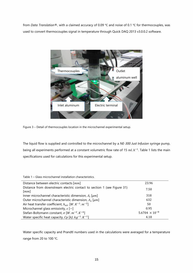
from Data Translation®, with a claimed accuracy of 0.09 ℃ and noise of 0.1 ℃ for thermocouples, was
used to convert thermocouples signal in temperature through Quick DAQ 2013 v3.0.0.2 software.
Figure 3 – Detail of thermocouples location in the microchannel experimental setup.
The liquid flow is supplied and controlled to the microchannel by a NE-300 Just Infusion syringe pump,
being all experiments performed at a constant volumetric flow rate of 15 𝑚𝑙. ℎ−1. Table 1 lists the main
specifications used for calculations for this experimental setup.
Table 1 – Glass microchannel installation characteristics.
Distance between electric contacts [𝑚𝑚] 23.96
Distance from downstream electric contact to section 1 (see Figure 31) [𝑚𝑚]
7.50
Inner microchannel characteristic dimension, 𝛬𝑖 [𝜇𝑚] 318
Outer microchannel characteristic dimension, 𝛬𝑜 [𝜇𝑚] 632
Air heat transfer coefficient, ℎ𝑎𝑖𝑟 [𝑊. 𝐾−1. 𝑚−2] 50
Microchannel glass emissivity, 휀 [−] 0.95
Stefan-Boltzmann constant, 𝜎 [𝑊. 𝑚−2. 𝐾−4] 5.6704 × 10⁻⁸
Water specific heat capacity, 𝐶𝑝 [𝑘𝐽. 𝑘𝑔−1. 𝐾−1] 4.18
Water specific capacity and Prandtl numbers used in the calculations were averaged for a temperature
range from 20 to 100 ℃.
Inlet aluminum
well
Outlet
aluminum well
Thermocouples
Electric terminal
16
In all the experiments involving technique parameters tests and in the calibration ones, it is necessary
to guarantee that the measurement point in the flow taken to test the technique is in a location
without gradients, either in space and time, assuring steady-state flow conditions. The hydrodynamic
and the thermal entrance lengths are, then, necessary to be determined prior to the experiments.
Hydrodynamic entrance length
The hydrodynamic entrance length of a flow represents the length in which the velocity profile
changes with position along the flow direction. From this distance on, a fully developed velocity profile
is verified and remains constant as far as no parameter in the flow is changed. The correlation
presented in Equation 18 has been proposed by Han [41] in 1960, to estimate the entrance length 𝐿𝐻𝑒
in micro square ducts with hydraulic diameters 𝐷ℎ smaller than 500 𝜇𝑚 over a range of Reynolds
numbers 𝑅𝑒 from 0.5 to 100.
𝐿𝐻𝑒
𝐷ℎ
=0.63
0.035 𝑅𝑒 + 1+ 0.0752 𝑅𝑒 Equation 18
For rectangular ducts,
𝐷ℎ =4 𝐴
𝑝 [𝑚] Equation 19
In the particular case of squared section ducts,
𝐷ℎ = 𝛬𝑖 [𝑚] Equation 20
where 𝛬𝑖 is the inner characteristic dimension of the channel.
The Reynolds number can be expressed as
𝑅𝑒 =𝑈 𝐷ℎ
𝜐 Equation 21
where 𝑈 is the flow average velocity [𝑚. 𝑠−1] which is obtained from the volumetric flow, 𝑄, using
Equation 22 and 𝜐 is the fluid kinematic velocity [𝑚2. 𝑠−1].
17
𝑄 = 𝐴 𝑈 [𝑚3. 𝑠−1] Equation 22
Thermal entrance length
From the heating zone inlet, heat is transported by the fluid gradually up to a point when the shape of
the temperature profile loses its identity and changes to a thermally fully developed region. The
distance from the heated region in which this phenomenon occurs is called thermal entrance length,
𝐿𝑇𝑒 [42], and can be estimated from
𝐿𝑇𝑒 = 0.01 𝑅𝑒 𝑃𝑟 𝐷ℎ [𝑚] Equation 23
for square ducts, where 𝑃𝑟 =𝑐𝑝𝜇
𝑘 is the Prandtl number and represents the ratio of momentum to
thermal diffusivity.
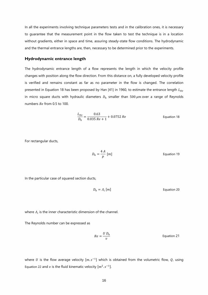
Figure 4 gives an example of microchannel wall temperature signal in time after a voltage is imposed
to the indium oxide layer terminals and shows that the flow reaches thermal steady state after 5
seconds.
Figure 4 – Example of temperature response after an imposed heat flux increase.

18
For the volumetric flow rate of 15 𝑚𝐿. ℎ−1 the maximum hydrodynamic entrance length, 𝐿𝑇ℎ, is
0.457 𝑚𝑚 and the maximum thermal entrance length, 𝐿𝑇𝑒 , is 0.295 𝑚𝑚 (𝜐 = 9.82 × 10⁻⁷𝑚2. 𝑠−1 and
𝑃𝑟 = 6.86). Thus, both velocity and thermal boundary layers are fully developed where visualization
and temperature measurements are taking place.
T-shaped micro-mixer
This is a simple flow configuration, which consists in the mixing between two liquid flows at different
temperatures in a T-shaped mixer, for the application of the present technique to measure 2D
temperature profiles at different flow regimes, but also of practical relevance to study mass and
thermal mixing at microscale.
Figure 5 – Schematics of the T-shaped micro-mixer experimental setup.
The experimental setup is schematically displayed in Figure 5 and consists of three silicon tubes, with
an internal diameter of 1 𝑚𝑚, pinched between two glass slides (detailed in Figure 6). An aqueous
solution with RhB at ambient temperature is supplied a NE-300 Just Infusion to the first inlet port, while
to the second inlet port is also supplied an aqueous RhB solution but at a higher temperature, pumped
Syringe pump
NE-300
K-type thermocouple
Inlet
C
Microscope
objective
HighSpeedStar 4G
CCD camera
DMIL LED
Microscope
Filter Cube
LED SFL100
Illumination
Reservoir
T-shaped
micro-mixer
Syringe pump
Harvard 22
Inlet
Pre-heater
Reservoir
Gear pump

19
by a Harvard 22 syringe pump, exiting the mixture through the third one. The mixing plane between
the hot and cold fluid streams for four different flow rates was visualized using a 4x/0.10 Leica
Microsystems objective lens, which is described in the following section.
Figure 6 – T-shaped micro-mixer scheme.
Hot fluid temperature is controlled in a secondary flow loop consisting of the custom made, thermally
isolated, acrylic reservoir shown in Figure 7, where two immersion resistances (1000 𝑊, model AI 03,
230 𝑉, 50 𝐻𝑧) controlled by an EGO Original 55.13022.060 thermostat (temperature range 30 – 110 ℃)
heat the water before it flows through silicon tubes encircling the primary flow loop.
Figure 7 – Secondary flow loop used to control the temperature of the hot flow. Reservoir, potentiometer and two
electric resistances.
𝑄𝐴𝑚𝑏
𝑄𝐻𝑜𝑡
𝑄𝐸𝑥𝑖𝑡

20
4.2 Equipment
The central part of the experimental facilities includes the LED illumination source, the CCD camera(s),
the microscope visualization system and the liquid pumping system(s). Temperature measurements are
performed to control and/or validate the optical temperature measurements in all experiments. For
that, precision fine wire type K thermocouples (Omega Engineering) with 25 𝜇𝑚 tip diameter are
placed either in contact with the solution and/or with the microchannel wall. An 8-channel isolated
thermocouple DAQ module, DT9828, from Data Translation®, with a claimed accuracy of 0.09 °C and
0.1 °C noise was used to convert the electrical signal of the thermocouples signal into temperature
through Quick DAQ 2013 v3.0.0.2 software.
Microscope
The microscope is the inverted fluorescence microscope Leica DM IL LED (Figure 8) with possibility to
interchange the objective lenses. Three lenses were then used: HI-PLAN 4x/0.10, HI-PLAN I 10x/0.22,
and N-PLAN EPI 20 x/0.40 from Leica and their suitability for the study was tested. The microscope can
also interchange sets of filter cubes. A LED SFL100 530 𝑛𝑚 size “s” set of filters was used.
Figure 8 – Leica DM IL inverted microscope. Image extracted from [43].

21
High speed cameras
Two high speed cameras were used to capture the fluorescence intensity signal, one for each dye.
HighSpeedStar camera from LaVision collected fluorescence information from RhB, while for Rh110
Phantom V4.2 from Vision Research was used.
The HighSpeedStar from LaVision, shown in Figure 9, is a high speed camera able to capture images at
a maximum rate of 3600 Hz with a resolution of 1024x1024 𝑝𝑖𝑥𝑒𝑙2 , which is connected to DMIL
microscope through a CCD adapter x0.55. A proprietary Software from LaVision, Davis8, is used to
acquire, save and export the images, as well as to trigger the whole setup through LaVision HighSpeed
controller.
Figure 9 – LaVision HighSpeedStar high speed camera with the x0.55 CCD adapter.
CCD adapter
Microscope
optics
HighSpeedStar
camera

22
To record the fluorescence signal emitted by the Rhodamine 110 solution, a Phantom V4.2 high speed
camera from Vision Research is used. This camera is attached to the custom made support shown in
Figure 10, purposely manufactured for this setup, to allow positioning the camera transversally to the
flow.
Prior to every experiment, a current session reference (calibration with black reference) with Phantom
Camera Control software has to be performed.
Figure 10 – Phantom v4.2 high speed camera and custom made support attached to the inverted microscope.
Custom
made
support
Melles Griot
16x/0.32
lens Melles Griot laser filter N-PLAN
20x/0.40
lens
Cosmicar CCD adapter
LED SFL100 530
𝑛𝑚 set of filters

23
Figure 11 – Rhodamine B filter characteristics. Transmission percentage as function of wavelength. (Chroma
Technology Corp., Scan range from 480.0 𝑛𝑚 to 680 𝑛𝑚, ET-TRITC Filter Set for 530 LED_Leica DMR_Un-Mounted).
To access the flow, a 16x/0.32 Melles Griot microscope objective lens is connected to a Cosmicar x2 TV
extender CCD adapter, then coupled to the camera. Between the lens and the flow a Melles Griot laser
filter 514.5 𝑛𝑚, with the transmission spectra shown in Figure 12, is precisely placed. Image acquisition,
saving and export are performed through Phantom Camera Control V.9.0.640.0-C software.
Figure 12 – Rhodamine 110 filter characteristics: Transmission percentage as function of wavelength. (Melles Griot
03FIL004 Laser Filter 514.5 𝑛𝑚 25 DIA, 03FIL00405100762).
Since both cameras have square pixels, sample density in x and y directions is the same. Both cameras
main characteristics are summarized in Table 2, according to manufacturer indications.
𝑊𝑎𝑣𝑒𝑙𝑒𝑛𝑔𝑡ℎ (𝑛𝑚)
%𝑇

24
Table 2 – Main characteristics of the high speed cameras used.
High Speed Camera
Characteristic
LaVision HighSpeedStar Vision Research Phantom V4.2
Maximum Resolution 1024x1024 pixel2 512x512 pixel2
Bits per sample 12 bits 8 bits
Exposure time 0.5 𝜇𝑠 80 𝜇𝑠
Acquisition rate 3600 Hz 2048 Hz
SNR (Equation 17) As both cameras have 𝑏 ≥ 8, quantization noise is negligible
To guarantee the accuracy of the optical arrangements, it is necessary to establish a relation between
the different optical arrangements and the size of the image being visualized. Making use of
calibration targets with well-defined mark spacing and precision dot patterning are represented in
Figure 13 a) and b), the HighSpeedStar camera calibration and the correspondence of pixel to image
size for both cameras can be determined, respectively. The spacing between dots in the target
represented in a) is of 20 𝜇𝑚 and the small lines in the reticle used represented in b) have a 100 𝜇𝑚
spacing.
a) b)
Figure 13 – HighSpeedStar calibration target from LaVision represented in a) and in b) the reticle from Peak Optics
used to establish the correspondence of pixel to image size for both cameras.
Results are presented in Table 3, with the respective depth of field, DOF, obtained by Equation 14.

25
Table 3 – Correspondence between the pixel and image size and depth of field in both high speed cameras for
different optical arrangements.
High Speed Camera
Arrangement
LaVision HighSpeedStar Vision Research Phantom V4.2
Pixel correspondent
size (𝜇𝑚) full
image size (𝑚𝑚)
DOF (𝜇𝑚)
Pixel correspondent
size (𝜇𝑚) full
image size (𝑚𝑚)
DOF (𝜇𝑚)
HI-PLAN 4x/0.10 with
x0.55 CCD adapter 7.69 7.87 97.95 – –
HI-PLAN I 10x/0.22 with
x0.55 CCD adapter 3.12 3.19 15.60 –
–
N-PLAN EPI 20 x/0.40 with
x0.55 CCD adapter 1.54 1.58 4.29 – –
Melles Griot 16x/0.32 with
x2 CCD adapter – – 2.09 1.07 6.36
Illumination system
The aqueous solutions containing fluorescent dyes are illuminated with the Leica illumination system
LED SFL100 530 𝑛𝑚 shown in Figure 14. This is a light source compatible with all microscopes
equipped for fluorescence, with low power consumption and represents an economic alternative to
traditional fluorescence microscopy setup. Despite light intensity can be adjustable, it was kept
constant during all experiments.

26
Figure 14 – Leica LED SFL100 illumination system.
Pumping systems
The flow(s) is/are pumped by a NE-300 syringe pump (Figure 15 a)) and/or a Harvard 22 syringe pump
(Figure 15 b)), both with an accuracy within ±1% over length of syringe, exclusive of syringe variations
and a reproducibility of ±0.1%. Solutions are prepared in flasks and then transferred to 60 𝑚𝐿 Norm-
Ject syringes. The syringe is connected to the installation through silicon piping and aluminium fittings.
a) b)
Figure 15 – Pumping systems: a) NE-300 syringe pump and b) Harvard 22 syringe pump.

27
4.3 Experimental method
One of the objectives of the present work is to compare the single dye method with the traditional
two-dye technique for microfluidic temperature measurements, as in [9]. Two dyes were then used,
RhB and Rh110, as temperature-sensitive and insensitive dyes, respectively.
Since LED-IFT uses intensity to measure temperature, a calibration is needed prior to applying the
technique, which takes into account for the losses of fluorescence intensity along the optical pathway
from the measurement volume to the CCD sensors.
The following paragraphs give the main characteristics of the fluorescence dyes and solutions followed
by a detailed description of the calibration setup, image processing and uncertainty estimation.
Fluorescent dyes
The accuracy of the Laser Induced Fluorescence relies on a particularly set of properties that particles
in solution must have. A summary of the most important optical characteristics of both dyes such as
absorption and emission wavelengths as well as quantum efficiency are summarized in Table 4.
Table 4 – Characteristics of aqueous solutions of Rhodamine B and Rhodamine 110 in de-ionized water at 20 ℃
(Adapted from [27] and [25])
Dye λabsorption [𝒏𝒎] λemission [𝒏𝒎] 𝚽 [–]
RhB 554 575 0.31
Rh110 496 520 0.8
Both dyes were purchased from Sigma-Aldrich and the aqueous solutions prepared (Table 5) using a
Mettler Toledo scale with accuracy and reproducibility of 0.1 mg. Figure 16 shows the visual aspect of
three of the solutions used in the experiments. Solutions containing RhB present a reddish tint, while
solutions with Rh110 shows a light green tone.

28
Figure 16 – Visual aspect of three solutions used. From left to right: RhB with a concentration of 20 mg.L-1; RhB
with a concentration of 20 mg.L-1 and Rh110 with a concentration of 15 mg.L-1; Rh110 with a concentration of
50 mg.L-1.
Mixtures of these solutions are prepared in order to obtain the desired solution concentrations
containing both dyes, following the relation:
𝐶𝑖𝑉𝑖 = 𝐶𝑓𝑉𝑓 Equation 24
where 𝐶 represents dye concentration and 𝑉 the volume, initial (𝑖) and final (𝑓). Two aqueous solutions
containing both dyes were prepared (see Table 5).
Table 5 – Aqueous solutions used in experiments.
RhB Concentration
[𝒎𝒈. 𝑳−𝟏] Rh110 Concentration
[𝒎𝒈. 𝑳−𝟏] RhB + Rh110 Concentrations
[𝒎𝒈. 𝑳−𝟏]
50
20 + 15
25 + 15
1.4
5
10
15
20
25
32.6
29
Calibration of the fluorescence intensity
The calibration consists in collecting the fluorescence intensity at known temperatures, which will allow
to convert the fluorescence signal into temperature (calibration curve) in further experiments.
As stated before in chapter 3, performing a normalization of the fluorescent signal retrieved from the
dyes makes the method needless of further calibration for different experimental setups.
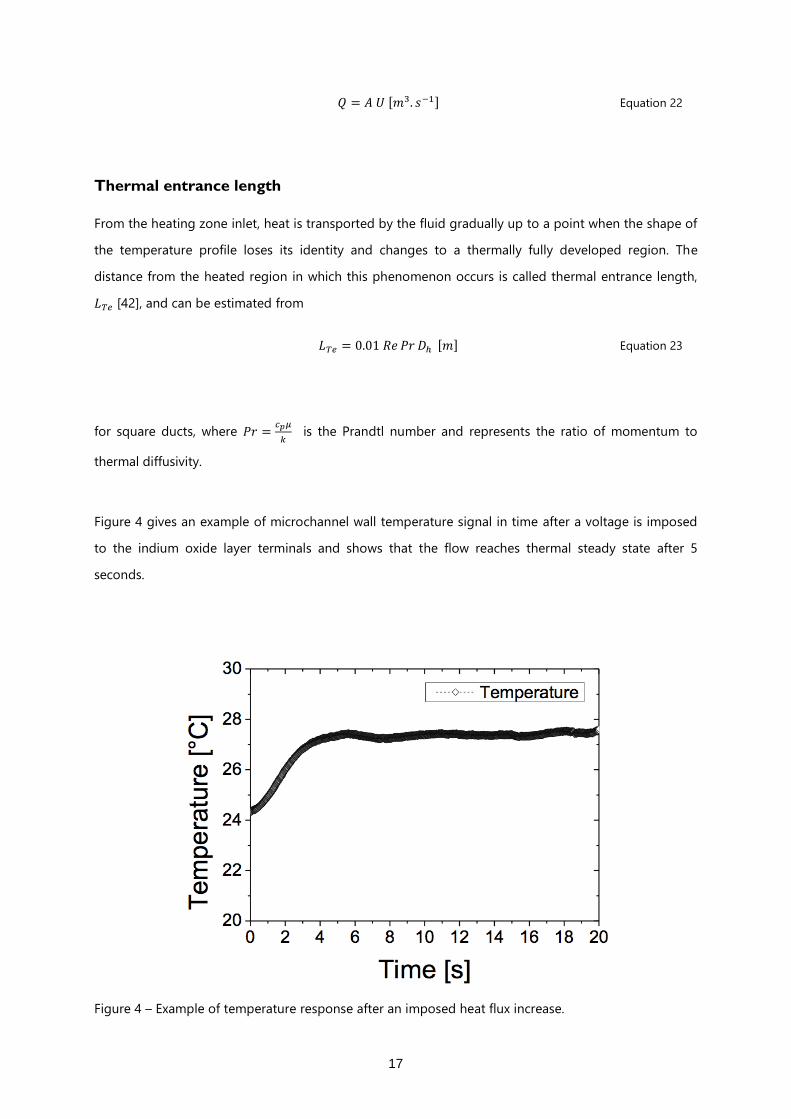
The calibration process requires precision for temperature control and measure, so a specific setup is
needed. As shown in Figure 17, it consists on a thermally insulated reservoir on top of a microscope
slide (76 × 26 𝑚𝑚2 × 1 ± 0.05 𝑚𝑚 thick) with a deposited indium oxide layer on the slide bottom in
order to vary the temperature of the dye solution by Joule effect and, at the same time, allowing
optical access from the bottom (the inverted DM IL LED microscope was used).
Figure 17 – Schematics of the thermally insulated pool.
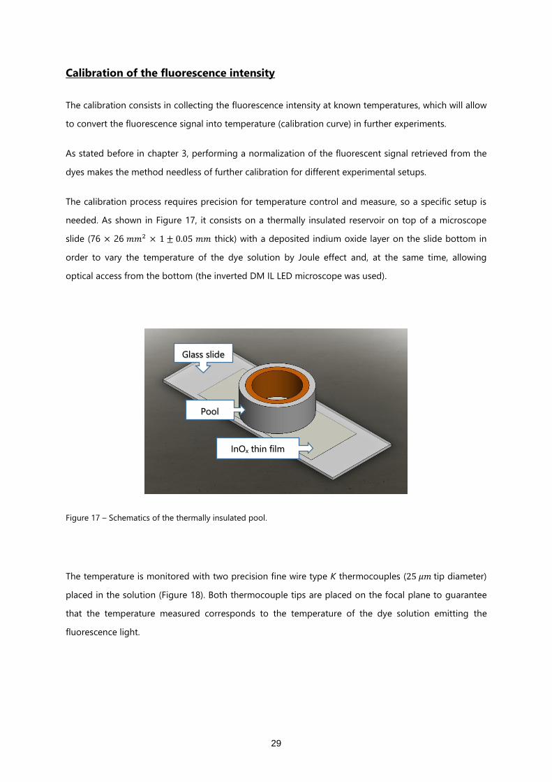
The temperature is monitored with two precision fine wire type K thermocouples (25 𝜇𝑚 tip diameter)
placed in the solution (Figure 18). Both thermocouple tips are placed on the focal plane to guarantee
that the temperature measured corresponds to the temperature of the dye solution emitting the
fluorescence light.
Pool
Glass slide
InOx thin film
30
Figure 18 – Schematics of the calibration setup.

31
The optical system makes use of the microscopic system described before: an inverted microscope DM
IL LED from Leica Microsystems equipped with the Leica HI PLAN I 10x/0.22 objective lens, and a 0.55x
amplifier tube connects the microscope to the HighSpeedStar 4G camera to collect the fluorescence
intensity signal from Rhodamine B, after being excited by the illumination system LED SFL100 530 𝑛𝑚
through size “S” set of filters from Leica Microsystems. Intensity in each 16-bit gray scale image was
acquired and exported to a .txt format using Davis 8 software from LaVision.
To simultaneously collect the signal emitted by Rhodamine 110, a 16x/0.32 Melles Griot objective lens
coupled to a Melles Griot laser filter 514.5 𝑛𝑚 are attached to a Phantom v4.2 high speed camera.
Phantom Camera Control Version 9.0.640.0-C software collects and saves the 8-bit grayscale images in
.bmp format.
The calibration process consists in filling the insulated pool with one or two dyes (depending on the
method) and applying a controlled voltage to the transparent thin film of Indium Oxide to heat the
solution up to the desired temperature. When fluid temperature stabilizes, temperature and
fluorescence intensity information are simultaneously collected.
Uncertainty estimates
The error expression adopted for this work was found in [44] and is described below. It has in
consideration the accuracy and the precision in measurements made, and runs
𝐸𝑟𝑟𝑜𝑟 = ±√𝐵2 + 2 × 𝜎2 Equation 25
where 𝐵 is the bias accuracy of the measurement device, 𝜎 is the standard deviation of the parameter
measurements, corresponding to the precision of measurements, and the constant 2 is a commonly
used constant to represent a 95% confidence interval with 4 degrees of freedom.
32
5. Results and Discussion
The experimental campaign starts with the calibration of the optical systems and tests to the different
parameters of the LED-IFT technique in the microchannel setup. Then the pool calibration setup
follows and the technique is applied to the two case studies: a training benchmark imposed to a
microchannel flow and flow inside a ‘T’-shaped micromixer.
This chapter is divided in two main sections. The first addresses the parameter optimization and
calibration of the LED-induced fluorescence system for temperature measurements; the second
considers the applications of the optimized configuration.
5.1. Test Parameters
The experiments for the technique parameters were performed in the fully developed region of a water
flow inside a microchannel with a constant heat flux at the wall. Rhodamine B and Rhodamine 110
dyes were used as temperature dependent and temperature independent dyes, respectively.
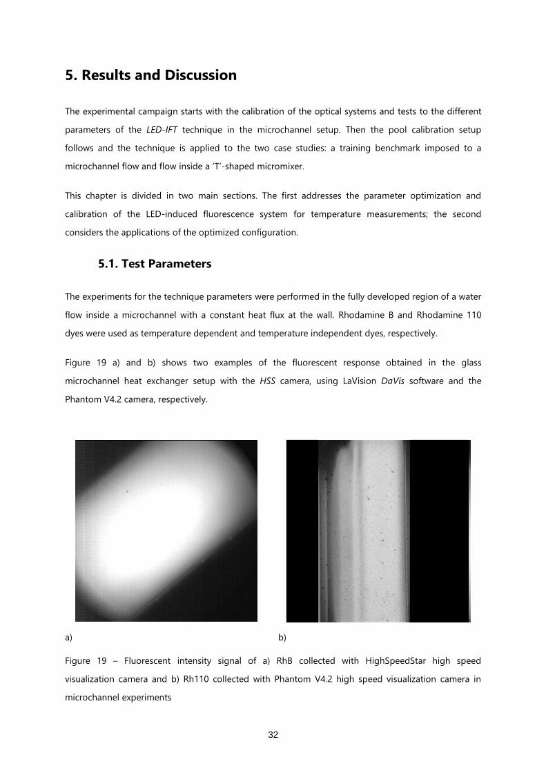
Figure 19 a) and b) shows two examples of the fluorescent response obtained in the glass
microchannel heat exchanger setup with the HSS camera, using LaVision DaVis software and the
Phantom V4.2 camera, respectively.
a) b)
Figure 19 – Fluorescent intensity signal of a) RhB collected with HighSpeedStar high speed
visualization camera and b) Rh110 collected with Phantom V4.2 high speed visualization camera in
microchannel experiments
33
Since HSS images have a tilt angle with respect to the channel, a small routine was implemented in
order to choose four equidistant control points in the image, from the centre of the channel, to
monitor the intensity across the experiments. The results are presented for only one control point, as
the results for the remaining control points are found to be similar (within deviations smaller than 10%
of the measured value) and, therefore, repeatable and reproducible. For the Pool Calibration System,
six randomly selected control points were chosen near the thermocouple tip to monitor the
fluorescence response, in order to obtain the calibration curve. Spatial and quantitative measurements
are intended for the T-shaped micro-mixer experiment, so all image pixels were considered.
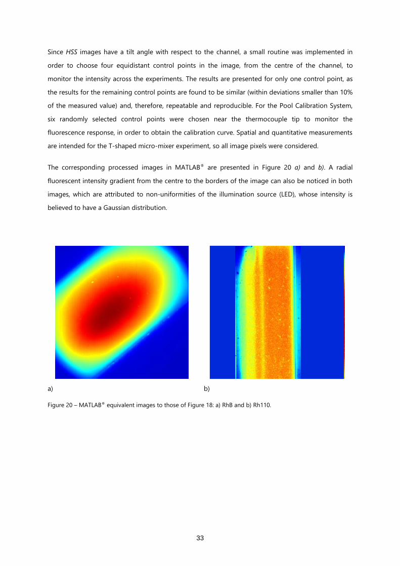
The corresponding processed images in MATLAB® are presented in Figure 20 a) and b). A radial
fluorescent intensity gradient from the centre to the borders of the image can also be noticed in both
images, which are attributed to non-uniformities of the illumination source (LED), whose intensity is
believed to have a Gaussian distribution.
a) b)
Figure 20 – MATLAB® equivalent images to those of Figure 18: a) RhB and b) Rh110.

34
Dye Concentration
Seven different concentrations of Rhodamine B were prepared and measurements taken for eight
different temperatures, obtained by applying eight different voltages to the Indium Oxide thin layer.
The results are depicted in Figure 21 and show the expected decrease of the fluorescence intensity as
the dye concentration decreases and temperature increases.
Figure 21 – Fluorescence intensity response obtained for the same control point for seven aqueous RhB solutions
with different concentrations.
The 𝑆𝑒𝑛𝑠𝑖𝑡𝑖𝑣𝑖𝑡𝑦 [%. ℃−1] of the technique is given by the gradient of the fluorescence intensity 𝑑𝐼 𝑑𝑇⁄
and can be written as a function of image intensity, 𝐼0, as
𝑆𝑒𝑛𝑠𝑖𝑡𝑖𝑣𝑖𝑡𝑦 =1
𝐼0
(𝑑𝐼
𝑑𝑇) × 100 Equation 26
As Rhodamine B concentration increases, the fluorescence signal also increases and with it the
temperature sensitivity. Figure 22 shows that the sensitivity increases almost linearly from 0.83 to a
maximum of 1.68 %. ℃−1 as dye concentration increases from 1.4 to 25 mg.L-1, after which it starts to
decrease.

35
Figure 22 – Influence of solution concentration in fluorescence signal sensitivity.
Therefore, a solution containing RhB with a concentration of 25 𝑚𝑔. 𝐿−1 was chosen for all the
subsequent experiments. The fluorescence signal of Rhodamine 110 was recorded with the Phantom
V4.2 high speed visualization camera: with a concentration of 15 𝑚𝑔. 𝐿−1, a sensitivity of 0.011% was
found, reflecting the independence of this dye fluorescence signal to temperature.
Influence of Background Noise
Another relevant parameter often mentioned in several studies as influencing the fluorescence signal is
the background noise present in the images caused by, either room illumination and/or static noise
induced by both camera and surroundings. Two set of experiments were performed to quantify this
influence: the first consists in comparing images collected with and without room illumination; the
second consists in subtracting an image obtained with the LED illumination source turned off to the
images collected with both, room and the LED illuminations on.
It is worth noting at this point that the second procedure will not be used with the Phantom camera
since its acquisition software always requires a current session reference before each measurement.
0 5 10 15 20 25 30 350.0
0.5
1.0
1.5
2.0
Sen
sitiv
ity [%
.ºC
-1]
Concentration [mg.L-1]

36
Figure 23 – Fluorescent signal from both dyes, for the same control point, with and without room illumination.
The results of the first set of experiments obtained with both, the HSS and the Phantom cameras, are
depicted in Figure 23, and show no significant dependence of the room illumination and, therefore, of
the background light. The results of the second set of experiments are summarized in Figure 24 and
show that subtracting the image obtained with the LED illumination source turned off only offsets the
original curve, and do not add any improvement.
Figure 24 – Rhodamine B fluorescent signal with and without background image removal.
20 30 40 50 60 70 80 900
200
400
600
800
1000
1200
1400
1600
Inte
nsity [A
.U.]
Temperature [°C]
RhB with room illumination
Rh110 with room illumination
RhB without room illumination
Rh110 without room illumination

37
Auto-absorption and Beer-Lambert Law
The last parameter to be tested before applying the LED-IFT technique is the influence of the auto-
absorption and reemission, as described in chapter 3. For that, experiments were performed with each
dye separately and the corresponding fluorescence signals were simultaneously captured with both
cameras. It is worth noting that, as already mentioned in the fluorescent dyes section, Rhodamine B
emits at a higher wavelength than the absorption wavelength of Rh110 and is, therefore, filtered by
the Rh110 filter, so there is no cross talk between the emission of RhB and the signal collected by the
Phantom V4.2 camera.
Figure 25 shows the fluorescence signal emitted by both Rh110 and RhB aqueous solutions obtained
at the same temperature conditions and captured with the HSS camera, first separately and after with
both dyes in solution, represented in black. At ambient temperature it is noticed an increase in
fluorescent signal intensity with both dyes in solution, when compared with only RhB fluorescent
signal, decreasing for higher solution temperatures. It is demonstrated then the auto-absorption and
reemission effects caused by the partial overlap between Rh110 emission and RhB absorption spectra
that can lead to image saturation problems, decreasing temperature sensitivity in the fluorescence
response obtained.
Figure 25 – Fluorescent signal on HSS image for both particles, separately and with both in solution.
20 30 40 50 60 70 80 900
200
400
600
800
1000
1200
1400
1600
Inte
nsity [A
.U.]
Temperature [°C]
Rh110 on HighSpeedStar
RhB on HighSpeedStar
RhB+Rh110 on HighSpeedStar

38
Calibration Curves – NR-LED-IFT vs N-LED-IFT
As mentioned before, there are essentially two ways to apply the LED Induced Fluorescence
Thermometry technique: the Normalized Image for Ratiometric LED-IFT (NR-LED-IFT) and the
Normalized LED-IFT (N-LED-IFT).
The pool calibration setup using both cameras was used in this set of experiments. As described
before, the heat flux applied to the microchannel flow can be controlled by varying the voltage applied
to the terminals of the indium oxide layer. The experiments are performed by increasing the voltage by
small steps (3V), only after reaching thermal steady-state conditions.
The intensity of the signals retrieved from both the HSS and Phantom cameras are shown in Figure 26.
The intensity difference between the control points within the same image, as explained in the
beginning of this section, is due to illumination non-uniformities caused by the Gaussian distribution
of the light source. The signal emitted by the temperature dependent dye (RhB) decreases as the
temperature increases from 1154 Arbitrary Units (𝐴. 𝑈.) at room temperature up to 253 𝐴. 𝑈. for 78.5℃,
which corresponds to a 78% change in fluorescence intensity. The signal emitted by the temperature
independent dye (Rh110) remains nearly constant, achieving a 2% maximum variation in fluorescence
intensity response along the temperature range tested, as expected.
Figure 26 – RhB and Rh110 fluorescence signal (FS) response to temperature.
20 30 40 50 60 70 80 900
200
400
600
800
1000
1200
1400
1600
Inte
nsity [A
.U.]
Temperature [°C]
HSS FS CP1
HSS FS CP2
HSS FS CP3
HSS FS CP4
Phantom FS CP1
Phantom FS CP2
Phantom FS CP3
Phantom FS CP4
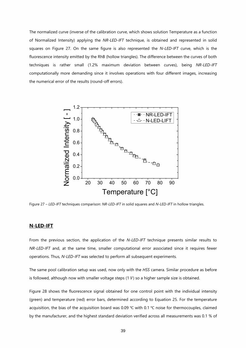
39
The normalized curve (inverse of the calibration curve, which shows solution Temperature as a function
of Normalized Intensity) applying the NR-LED-IFT technique, is obtained and represented in solid
squares on Figure 27. On the same figure is also represented the N-LED-IFT curve, which is the
fluorescence intensity emitted by the RhB (hollow triangles). The difference between the curves of both
techniques is rather small (1.2% maximum deviation between curves), being NR-LED-IFT
computationally more demanding since it involves operations with four different images, increasing
the numerical error of the results (round-off errors).
Figure 27 – LED-IFT techniques comparison: NR-LED-IFT in solid squares and N-LED-IFT in hollow triangles.
N-LED-IFT
From the previous section, the application of the N-LED-IFT technique presents similar results to
NR-LED-IFT and, at the same time, smaller computational error associated since it requires fewer
operations. Thus, N-LED-IFT was selected to perform all subsequent experiments.
The same pool calibration setup was used, now only with the HSS camera. Similar procedure as before
is followed, although now with smaller voltage steps (1 𝑉) so a higher sample size is obtained.
Figure 28 shows the fluorescence signal obtained for one control point with the individual intensity
(green) and temperature (red) error bars, determined according to Equation 25. For the temperature
acquisition, the bias of the acquisition board was 0.09 ℃ with 0.1 ℃ noise for thermocouples, claimed
by the manufacturer, and the highest standard deviation verified across all measurements was 0.1 % of
20 30 40 50 60 70 80 900.0
0.2
0.4
0.6
0.8
1.0
1.2
Norm
aliz
ed Inte
nsity [ -
]
Temperature [°C]
NR-LED-IFT
N-LED-LIFT

40
the temperature measured. As for the intensity information, the standard deviation for each set of 50
images was determined. The error obtained for intensity measurements is of 1.5 % for solution at
ambient temperature and increases up to 3.8 % for 92 ℃, as for temperature the error goes from 0.19
to 0.23 ℃, with temperature increasing from 27 ℃ to 92 ℃, corresponding to a maximum relative error
of 0.71% for the lower temperature.
Figure 28 – RhB fluorescence signal collected in the Pool Calibration system.
Normalized fluorescence signal from RhB dye particles for 6 different control points is represented in
Figure 29. As it can be seen, despite the non-uniformities in the illumination system, all six normalized
curves overlap, validating the illumination independence of the method.
The calibration curve is obtained by inverting the normalized curve as presented in Figure 30. A forth
order polynomial that best fits the results with a correlation factor near the unity is also presented so a
continuous range of temperatures for a continuous range of normalized intensities is obtained. A table
with the polynomial characteristics is also shown in the same figure, including the standard deviations
for its coefficients.
30 40 50 60 70 80 90200
400
600
800
1000
1200
Inte
nsi
ty [A
.U.]
Temperature [°C]
Experimental data
Temperature error
Intensity error

41
Figure 29 – Normalized intensity for 6 different control points.
It is worth noting that the polynomial shown is a best-fit for the experimental results, thus special
attention must be paid when applying it with normalized intensity values outside the calibration data
range. Because robustness is needed, the polynomial inflection points are determined so the range of
normalized intensities is limited accordingly, and no major extrapolation errors were observed.
Figure 30 – Calibration curve for the N-LED-IFT technique with a 4th order best fit polynomial.
20 30 40 50 60 70 80 900.0
0.2
0.4
0.6
0.8
1.0
1.2
Norm
aliz
ed Inte
nsi
ty [ -
]
Temperature [°C]
CP 1
CP 2
CP 3
CP 4
CP 5
CP 6
0.0 0.2 0.4 0.6 0.8 1.0 1.20
20
40
60
80
100
Te
mp
era
ture
[°C
]
Normalized Intensity [ - ]
Calibration Experimental Data
Polynomial Fit
Model Polynomial
Adj. R-Square 0.99904
Value Standard Error
Temperature Intercept 149.52582 3.28655
Temperature B1 -381.13887 28.37796
Temperature B2 603.42819 84.99966
Temperature B3 -533.38187 105.58829
Temperature B4 189.61135 46.31142
𝑇 [℃] = 189.6 × 𝑁𝐼4 − 533.4 × 𝑁𝐼3 + 603.4 × 𝑁𝐼2
− 381.1 × 𝑁𝐼 + 149.5

42
5.2. Application of the LED-IFT technique
The results in the previous section showed that the N-LED-IFT technique is the most advantageous.
This chapter addresses the results obtained with this technique applied in two proof-of-concept tests
of different nature, the Training Benchmark applied to the microchannel and the T-shaped micro-
mixer, aiming at discussing the accuracy of the technique to measure temperature distributions in
microflows.
Training Benchmark
The experimental setup used in this application is that described in section 4.1 and shown in Figure 2.
The flow conditions consisted in applying different voltages to the indium oxide layer deposited in the
microchannel outer wall and measuring the fluorescence response, which is later compared with a
simplified theoretical model. This is the benchmark test usually applied to computer chips to track CPU
utilization and performance.
The configuration of the flow is shown in Figure 31, where can be seen the location of two
thermocouples, in 1 and 2, which allow measuring the temperature in the microchannel wall in two
different sections. In the following, subscript 2 refer to the temperature measured in the microchannel
wall in section 2 and subscript 𝑣 represents the fluid temperature measured by the N-LED-IFT
technique in the visualization section, v.
The outer wall of the microchannel is heated by Joule effect with the current supplied by the Gen 150-
5 power supply, with a power output, 𝑃, that can be determined from the product of voltage, 𝑉, by the
current intensity, 𝐼, both acquired from GenesysControl software:
𝑃 = 𝑉𝐼 Equation 27
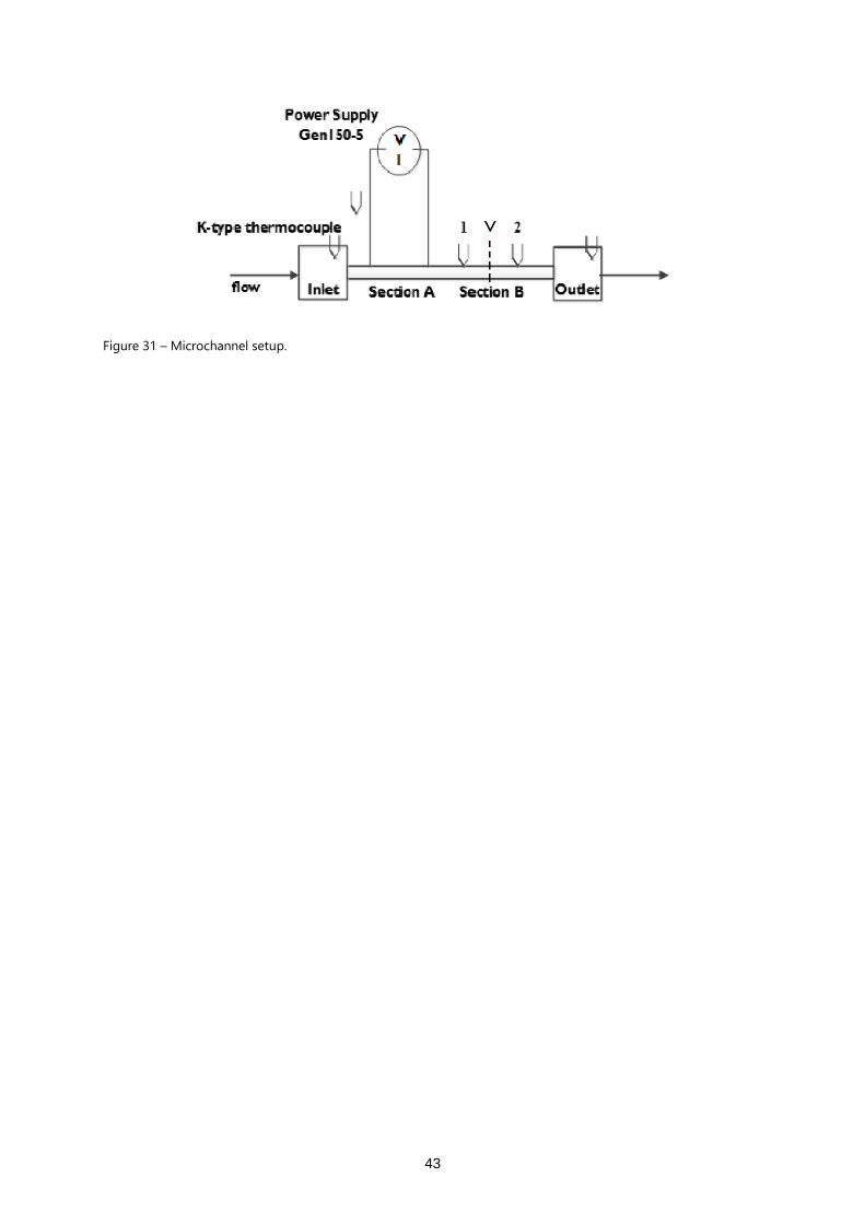
43
Figure 31 – Microchannel setup.
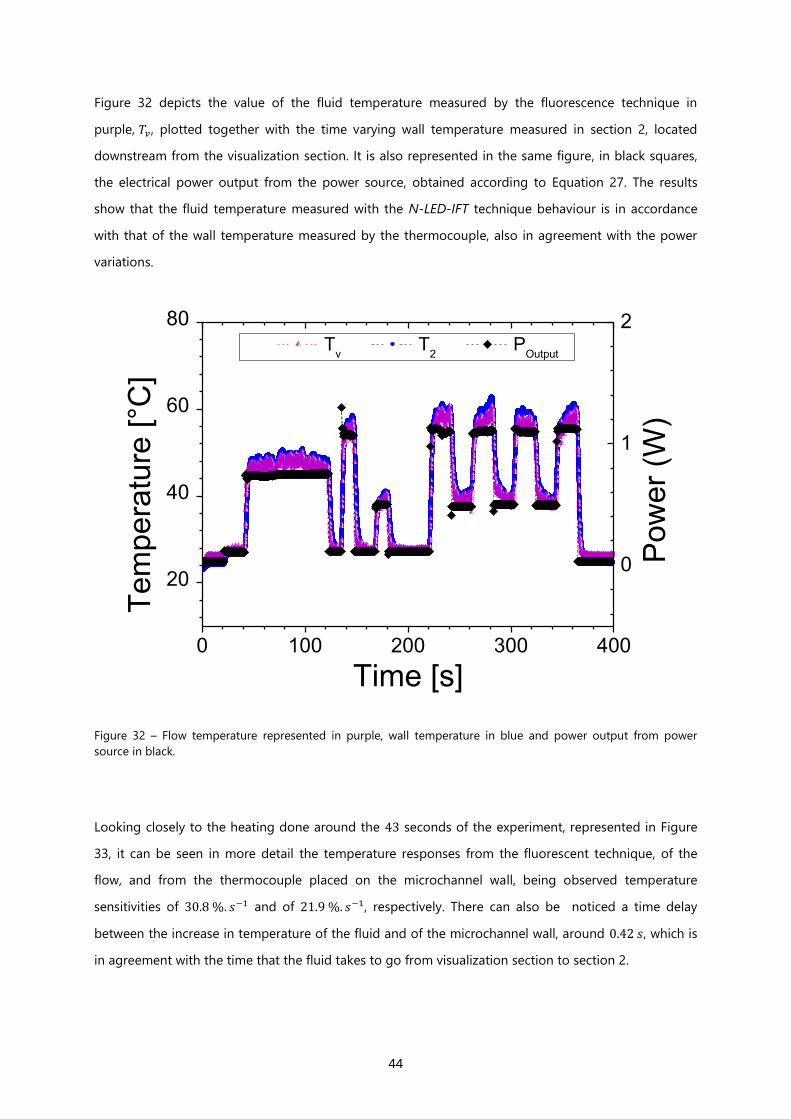
44
Figure 32 depicts the value of the fluid temperature measured by the fluorescence technique in
purple, 𝑇𝑣, plotted together with the time varying wall temperature measured in section 2, located
downstream from the visualization section. It is also represented in the same figure, in black squares,
the electrical power output from the power source, obtained according to Equation 27. The results
show that the fluid temperature measured with the N-LED-IFT technique behaviour is in accordance
with that of the wall temperature measured by the thermocouple, also in agreement with the power
variations.
Figure 32 – Flow temperature represented in purple, wall temperature in blue and power output from power
source in black.
Looking closely to the heating done around the 43 seconds of the experiment, represented in Figure
33, it can be seen in more detail the temperature responses from the fluorescent technique, of the
flow, and from the thermocouple placed on the microchannel wall, being observed temperature
sensitivities of 30.8 %. 𝑠−1 and of 21.9 %. 𝑠−1, respectively. There can also be noticed a time delay
between the increase in temperature of the fluid and of the microchannel wall, around 0.42 𝑠, which is
in agreement with the time that the fluid takes to go from visualization section to section 2.
0 100 200 300 400
20
40
60
80
Tv T
2 P
Output
Te
mp
era
ture
[°C
]
Time [s]
0
1
2
Pow
er
(W)

45
Figure 33 – Detail on the responses from the N-LED-IFT technique and from the thermocouple measurements for
a power increase.
T-shaped micro-mixer
One of the great advantages of the LED-IFT technique is to be able to obtain 2D fluid temperature
profiles, which are difficult to obtain through traditional temperature measurement techniques as
thermocouples. The suitability of N-LED-IFT method for temperature measurements in microchannel
applications is tested through quantitative visualization of the temperature field in a mixing plane
obtained by driving a hot and a cold fluid stream together in a T-shaped micro mixer.
In Figure 34 the mixing plane for three different volumetric flows is depicted. A lighter (hotter) fluid jet
is observed to flow across the main cold flow stream. Despite small temperature differences between
the two fluid streams, entering at 35 and 24 ℃, contact zones between them are well defined. By
varying the volumetric flow rate from 𝑄𝑐𝑜𝑙𝑑 = 200 𝑚𝐿. ℎ−1 and 𝑄ℎ𝑜𝑡 = 200 𝑚𝐿. ℎ−1 (Figure 34 a), to
𝑄𝑐𝑜𝑙𝑑 = 300 𝑚𝐿. ℎ−1 and 𝑄ℎ𝑜𝑡 = 300 𝑚𝐿. ℎ−1 (Figure 34 b) is evident the movement from the mixing of
both flows to a region further away from the hot fluid inlet, with a higher curve angle when
𝑄𝑐𝑜𝑙𝑑 = 500 𝑚𝐿. ℎ−1 𝑄ℎ𝑜𝑡 = 50 𝑚𝐿. ℎ−1 (Figure 34 c).

46
a) b) c)
Figure 34 – Mixing plane of two laminar stream flows with different velocities: a) 𝑄𝑐𝑜𝑙𝑑 = 200 𝑚𝑙. ℎ−1, 𝑄ℎ𝑜𝑡 =
200 𝑚𝑙. ℎ−1; b) 𝑄𝑐𝑜𝑙𝑑 = 300 𝑚𝑙. ℎ−1, 𝑄ℎ𝑜𝑡 = 300 𝑚𝑙. ℎ−1; c) 𝑄𝑐𝑜𝑙𝑑 = 500 𝑚𝑙. ℎ−1, 𝑄ℎ𝑜𝑡 = 50 𝑚𝑙. ℎ−1. Cold fluid
coming from left to right and hot fluid inlet is on the top.
Increasing the volumetric flow rate, Reynolds number increases, which after some point is reflected in
flow properties modifications. Results are shown in Figure 35. Images were captured for
𝑄𝑐𝑜𝑙𝑑 = 1000 𝑚𝑙. ℎ−1 and 𝑄ℎ𝑜𝑡 = 1000 𝑚𝑙. ℎ−1 with a 5 𝑚𝑠 difference between each image. It can be
noticed that the high spatial resolutions obtained with this temperature measurement technique are
able to retrieve detailed temperature information in the resulting vortexes, and capture the evolution
of heat transfer phenomena in flows with this characteristics in such short timescales.
a) b) c)
Figure 35 – Mixing plane of two stream flows for the same volumetric flow, 𝑄𝑐𝑜𝑙𝑑 = 1000 𝑚𝑙. ℎ−1 and 𝑄ℎ𝑜𝑡 =
1000 𝑚𝑙. ℎ−1. Consecutive images captured with a 200 𝐻𝑧 acquisition rate. Cold fluid coming from the left to the
right and hot fluid inlet on the top.

47
6. Concluding Remarks and Future Work
In this study two LED-IFT techniques were described, tuned and applied to microscale flows in a
microchannel and in a T-shaped junction using a LED SFL100 530 𝑛𝑚 as illumination source.
Rhodamine B and Rhodamine 110 were used as temperature sensitive and temperature insensitive
dyes, respectively. Several parameters impacting the technique implementation were addressed and a
comparison between N-LED-IFT and NR-LED-IFT was performed. Results indicated no straight
advantage in using an extra dye, requiring more computer time/memory capability and adding
computational errors in the process, so N-LED-IFT was chosen to proceed with experiments.
Flow temperatures measured with the N-LED-IFT technique showed similar behaviour with the
microchannel wall temperature measured by the thermocouple. It was verified a time delay between
temperature responses that is in agreement with the time that the fluid takes from visualization to
thermocouple’s section. The capability of this technique to be applied to low and high velocity
microscale flows using a LED illumination source was demonstrated. 2D fluid temperature profiles
where obtained with high spatial (1.54m) and temporal (5 𝑚𝑠) resolutions, being the last one possible
to be increased with higher acquisition rates supported by the highspeed camera. LED illumination
being more stable, less expensive and energy consuming, and at the same allowing a wider range of
wavelengths to appropriately match the maximum wavelength for the fluorescence of the dye,
presents an alternative to lasers in fluorescence based techniques.
Precision and accuracy are directly related with the equipment used for image acquisition and
temperature measurement for the calibration curve. A thorough calibration process was performed
and found crucial to obtain quality results. The results presented showed errors lower than 3.8 % in
fluorescence intensity and lower than 0.71 % in temperature measurements. Call of attention upon the
fact that reference temperatures for the calibration and for the measurements normalization images
must be the same.
Although LED-IFT related errors can be reduced by averaging results over larger areas, consequently
reducing the effect of possible noise present in data acquired, for non-stationary conditions averaging
over large areas will lead to information loss as seen after some preliminary processing. All results
presented in this study are therefore obtained from single-pixel information.
As recommendation for future work, it would be interesting to use another calibration system and/or
illumination source to infer about the influence of those in experimental results, also validating the

48
results presented in this work. Other influencing parameters, such as photo bleaching could become
more relevant and should also be addressed.
In order to validate the results from any LED-IFT technique it is necessary to make use of
Computational Fluid Dynamics (CFD) tools to compare the results obtained from the technique. Also,
studies involving heat transfer in microscale turbulent flows with 2D temperature visualization can
provide better understanding to such complex phenomena.

49
References
[1] S. G. Kandlikar and W. J. Grande, “Evaluation of Single Phase Flow in Microchannels for High Heat Flux
Chip Cooling—Thermohydraulic Performance Enhancement and Fabrication Technology,” Heat Transf.
Eng., vol. 25, no. 8, pp. 5–16, Dec. 2004.
[2] D. B. Tuckerman and R. F. W. Pease, “High-performance heat sinking for VLSI,” IEEE Electron Device
Lett., vol. 2, no. 5, pp. 126–129, May 1981.
[3] C. B. Sobhan and S. V. Garimella, “A Comparative Analysis of Studies on Heat Transfer and Fluid Flow
in Microchannels,” Microscale Thermophys. Eng., vol. 5, no. 4, pp. 293–311, Oct. 2001.
[4] S. Garimella and C. Sobhan, “Transport in microchannels - A critical review,” Annu. Rev. heat Transf., pp.
1–50, 2003.
[5] V. K. Natrajan and K. T. Christensen, “Two-color laser-induced fluorescent thermometry for
microfluidic systems,” Meas. Sci. Technol., vol. 20, no. 1, p. 015401, Jan. 2008.
[6] L. N. Sanford and C. T. Wittwer, “Monitoring temperature with fluorescence during real-time PCR and
melting analysis,” Anal. Biochem., vol. 434, no. 1, pp. 26–33, Mar. 2013.
[7] S. V. Garimella, “Advances in mesoscale thermal management technologies for microelectronics,”
Microelectronics J., vol. 37, no. 11, pp. 1165–1185, Nov. 2006.
[8] S. G. Kandlikar and A. V. Bapat, “Evaluation of jet impingement, spray and microchannel chip cooling
options for high heat flux removal,” Heat Transf. Eng., vol. 28, no. 11, pp. 911–923, Nov. 2007.
[9] P. Chamarthy, S. V. Garimella, and S. T. Wereley, “Measurement of the temperature non-uniformity in
a microchannel heat sink using microscale laser-induced fluorescence,” Int. J. Heat Mass Transf., vol. 53,
no. 15–16, pp. 3275–3283, Jul. 2010.
[10] P.-S. Lee, S. V. Garimella, and D. Liu, “Investigation of heat transfer in rectangular microchannels,” Int. J.
Heat Mass Transf., vol. 48, no. 9, pp. 1688–1704, Apr. 2005.
[11] S. P. Jang, S. J. Kim, and K. W. Paik, “Experimental investigation of thermal characteristics for a
microchannel heat sink subject to an impinging jet, using a micro-thermal sensor array,” Sensors
Actuators A Phys., vol. 105, no. 2, pp. 211–224, Jul. 2003.
[12] T. Chen and S. V. Garimella, “Measurements and high-speed visualizations of flow boiling of a dielectric
fluid in a silicon microchannel heat sink,” Int. J. Multiph. Flow, vol. 32, no. 8, pp. 957–971, Aug. 2006.
[13] J.-H. Tsai and L. Lin, “Transient thermal bubble formation on polysilicon micro-resisters,” J. Heat
Transfer, vol. 124, no. 2, p. 375, 2002.
[14] T. Astarita, G. Cardone, G. M. Carlomagno, C. Meola, M. Melloni, G. Kirchho, C. Maxwell, J. Stefan, L.
Boltzmann, and M. Planck, “A survey on infrared thermography for convective heat transfer
measurements,” Opt. Laser Technol., vol. 32, no. 2000, pp. 593–610, 2001.
[15] G. Hetsroni, a. Mosyak, E. Pogrebnyak, and R. Rozenblit, “Infrared temperature measurements in
micro-channels and micro-fluid systems,” Int. J. Therm. Sci., vol. 50, no. 6, pp. 853–868, Jun. 2011.
[16] M. Wae-hayee, P. Tekasakul, S. Eiamsa-ard, and C. Nuntadusit, “Effect of cross-flow velocity on flow
and heat transfer characteristics of impinging jet with low jet-to-plate distance,” J. Mech. Sci. Technol.,
vol. 28, no. 7, pp. 2909–2917, Jul. 2014.
50
[17] V. U. Kakade, G. D. Lock, M. Wilson, J. M. Owen, and J. E. Mayhew, “Accurate heat transfer
measurements using thermochromic liquid crystal. Part 1: Calibration and characteristics of crystals,”
Int. J. Heat Fluid Flow, vol. 30, no. 5, pp. 939–949, Oct. 2009.
[18] C. D. Richards, R. F. Richards, and S. Boltzman, “Transient temperature measurements in a
convectively cooled droplet,” Exp. Fluids, vol. 25, 1998.
[19] T.-Y. Lin and S. G. Kandlikar, “Heat Transfer Investigation of Air Flow in Microtubes-Part II: Scale and
Axial Conduction Effects.,” J. Heat Transfer, vol. 135, no. 3, pp. 317041–317046, Mar. 2013.
[20] N. Omenetto, P. Benetti, and G. Rossi, “Flame temperature measurements by means of atomic
fluorescence spectrometry,” Spectrochim. Acta Part B At. Spectrosc., vol. 27, no. 10, pp. 453–461, Oct.
1972.
[21] C. Chan and J. W. Daily, “Measurement of temperature in flames using laser induced fluorescence
spectroscopy of OH,” Appl. Opt., vol. 19, no. 12, pp. 1963–1968, 1980.
[22] T. Nakajima, M. Utsunomiya, and Y. Ikeda, “Simultaneous Measurement of Velocity and Temperature of
Water Using LDV and Fluorescence Technique,” in Applications of Laser Techniques to Fluid Mechanics
SE - 3, R. J. Adrian, D. F. G. Durão, F. Durst, M. Maeda, and J. Whitelaw, Eds. Springer Berlin
Heidelberg, 1991, pp. 34–53.
[23] J. Sakakibara, K. Hishida, and M. Maeda, “Experiments in Fluids Measurements of thermally stratified
pipe flow using image-processing techniques,” Exp. Fluids, vol. 96, pp. 82–96, 1993.
[24] J. Sakakibara, K. Hishida, and M. Maeda, “Vortex structure and heat transfer in the stagnation region of
an impinging plane jet (simultaneous measurements of velocity and temperature fields by digital particle
image velocimetry and laser-induced fluorescence),” Int. J. Heat Mass Transf., vol. 40, no. 13, pp. 3163–
3176, Sep. 1997.
[25] T. L. Arbeloa, M. J. T. Estévez, F. L. Arbeloa, I. U. Aguirresacona, and I. L. Arbeloa, “Luminescence
properties of rhodamines in water/ethanol mixtures,” J. Lumin., vol. 48 & 49, pp. 400–404, 1991.
[26] J. Coppeta and C. Rogers, “Dual emission laser induced fluorescence for direct planar scalar behavior
measurements,” Exp. Fluids, vol. 25, no. 1, pp. 1–15, Jun. 1998.
[27] J. Sakakibara and R. J. Adrian, “Whole field measurement of temperature in water using two-color laser
induced fluorescence,” Exp. Fluids, vol. 26, no. 4941, 1999.
[28] P. Lavieille, A. Delconte, D. Blondel, M. Lebouché, and F. Lemoine, “Non-intrusive temperature
measurements using three-color laser-induced fluorescence,” Exp. Fluids, vol. 36, no. 5, pp. 706–716,
May 2004.
[29] M. Bruchhausen, F. Guillard, and F. Lemoine, “Instantaneous measurement of two-dimensional
temperature distributions by means of two-color planar laser induced fluorescence (PLIF),” Exp. Fluids,
vol. 38, no. 1, pp. 123–131, Dec. 2004.
[30] D. Ross, M. Gaitan, and L. E. Locascio, “Temperature measurement in microfluidic systems using a
temperature-dependent fluorescent dye.,” Anal. Chem., vol. 73, no. 17, pp. 4117–23, Sep. 2001.
[31] S. Y. Yoon and K. C. Kim, “Signal intensity enhancement of μ-LIF by using ultra-thin laser sheet
illumination and aqueous mixture with ethanol/methanol for micro-channel applications,” Opt. Lasers
Eng., vol. 44, no. 3–4, pp. 224–239, Mar. 2006.
[32] J. Sakakibara and R. J. Adrian, “Measurement of temperature field of a Rayleigh-Bénard convection using
two-color laser-induced fluorescence,” Exp. Fluids, vol. 37, no. 3, pp. 331–340, Jul. 2004.

51
[33] I. S. Burns and C. F. Kaminski, “Diode Laser Induced Fluorescence for Gas-Phase Diagnostics,”
Zeitschrift für Phys. Chemie, vol. 225, no. 11–12, pp. 1343–1366, Dec. 2011.
[34] A. Rodat-Boutonnet, P. Naccache, A. Morin, J. Fabre, B. Feurer, and F. Couderc, “A comparative study
of LED-induced fluorescence and laser-induced fluorescence in SDS-CGE: application to the analysis of
antibodies.,” Electrophoresis, vol. 33, no. 12, pp. 1709–14, Jul. 2012.
[35] J. V. do N. Palmeira, “Desenvolvimento e optimização de um sensor de fibra óptica para determinação
da concentração de oxigénio,” Universidade de Lisboa, Faculdade de Ciências e Tecnologia, 2009.
[36] J. Vogt, “Development of novel Particle Image Thermometry methods for highly resolved
measurements of temperature and velocity fields in fluids,” TU Darmstadt, 2014.
[37] Inoué, Shinya, Spring, and Kenneth, Video Microscopy: The Fundamentals, 2nd ed. New York: Springer
Berlin Heidelberg, 1997, p. 742.
[38] C. D. Meinhart, S. T. Wereley, and M. H. B. Gray, “Volume illumination for two-dimensional particle
image velocimetry,” Meas. Sci. Technol., vol. 11, no. 6, p. 809, 2000.
[39] S. L. Ellenberger, Influence of Defocus on Measurements in Microscope Images, Volume 51 . ASCI, 2000,
2000, p. 160.
[40] V. Silvério, A. L. N. Moreira, V. Semião, C. A. N. de Carvalho, G. Lavareda, P. Parreira, and A. Amaral,
“Heat transfer investigations in micro-channel flows,” in 15th Int Symp on Applications of Laser Techniques
to Fluid Mechanics, 2010.
[41] L. S. Han, “Hydrodynamic Entrance Lengths for Incompressible Laminar Flow in Rectangular Ducts,” J.
Appl. Mech., vol. 27, no. 3, pp. 403–409, Sep. 1960.
[42] W. Kays, M. Crawford, H. Iacovides, F. P. Incropera, D. P. DeWitt, T. L. Bergman, and A. S. Lavine,
Convective heat and mass transfer, vol. 6th. 1993, p. 137.
[43] “Leica DM IL inverted microscope.” [Online]. Available:
http://cfnewsads.thomasnet.com/images/large/553/553860.jpg. [Accessed: 01-Sep-2014].
[44] R. B. Abernethy, R. P. Benedict, and R. B. Dowdell, “ASME Measurement Uncertainty,” J. Fluids Eng., vol.
107, no. 2, pp. 161–164, Jun. 1985.

52
Appendix
Processing algorithm
A custom made MATLAB® program reads and processes the fluorescence intensity information as well
as the temperature information as described:
% Import data from experiments
If experiment == Dynamic %non-stationary experiments in which fluorescence is monitored over time
Asks for data directory;
Asks for experiment parameters;
Imports data (.txt or .bmp);
Saves data on a structure;
Else
Asks for how many measurements within same experiment and its parameters;
Asks for data directories;
For j = 1 : number of directories
For i = 1 : number of files in each directory
Imports data (.txt or .bmp);
{Intensity on each position} = read i data;
End
Average intensity on each position = mean (intensity on each position);
Standard deviation of Intensity on each position = std (Intensity on each position);
End
Saves data on a structure;
End
If experiment == Test Parameter % usage of control points to monitor parameters influence
Asks for name of the structure containing data;
Asks for the coordinates of opposite edges of the microchannel section;
Calculate central, equally spaced control points;
Creates intensity vectors for each control point;
If plot == Intensity vs Temperature

53
Creates an Intensity vs Temperature plot for the different control points;
Else if plot == Normalized Intensity vs Temperature
Asks for the structure and the name of the reference image;
Performs intensity vectors normalization; % N-LED-IFT or NR-LED-IFT
Creates a Normalized Intensity vs Temperature plot for the different control points;
End
Else if experiment == Calibration
Asks for name of the structure containing the normalized data for the calibration curve;
Asks for the coordinates of the desired control points;
Creates normalized intensity vectors for each control point;
Creates a Normalized Intensity vs Temperature plot for the different control points;
Else if experiment == Dynamic
% Temperature data
For n = 1 : number of voltage steps
Temperature ( n ) = mean (temperature collected for each voltage step);
Standard deviation of Temperature ( n ) = std (temperature collected for each voltage
step);
End
% Imaging data
Asks for the structure and the name of the reference image;
Performs intensity matrices normalization; % N-LED-IFT or NR-LED-IFT
Converts normalized intensity matrices in temperature ones;
Saves temperature matrices in a structure;
End


