
Lind on Measuring Benefits
© Allen C. Goodman, 2009
Suppose
• We have 2 types of land, half polluted (p), half not (u).
• Pp = 100; Pu = 200• If a program of air pollution
control equalizes productivity everywhere, rent may end up at 150.
• If so total property values remain same.
• Does this mean there were no benefits?

Diagram
200
100
Pp Pu
100 100 200
150
Analysis
• Assume class of programs w/ output specific to particular locations.
• How do we measure benefits?
• Two major findings– Benefits of a project can be approximating by measuring net
increase in profits of activities located on land directly affected by project.
– W/ zero profits, total change in productivity equals change in land values.
Analysis
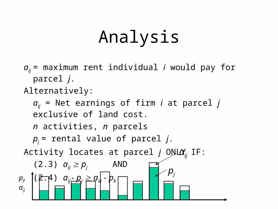
aij = maximum rent individual i would pay for parcel j.
Alternatively:
aij = Net earnings of firm i at parcel j exclusive of land cost.
n activities, n parcels
pj = rental value of parcel j.
Activity locates at parcel j ONLY IF:
(2.3) aij pj AND
(2.4) aij - pj aik - pk pj,aij
aij
pj
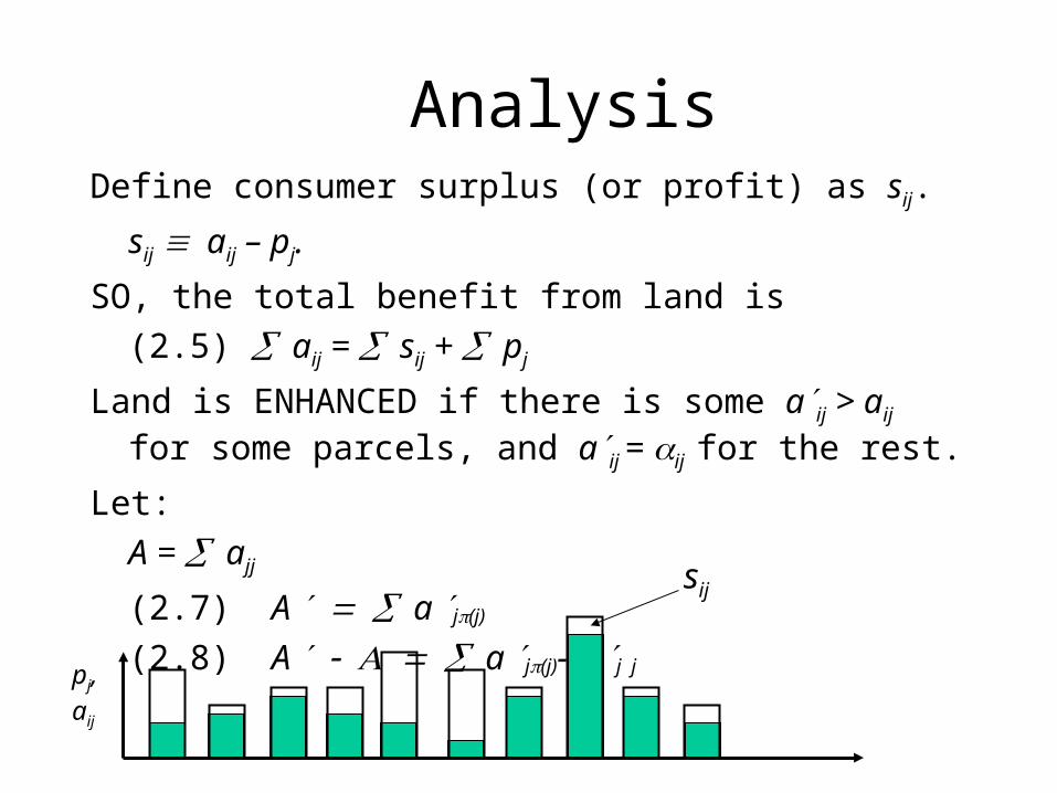
AnalysisDefine consumer surplus (or profit) as sij.
sij aij – pj.
SO, the total benefit from land is
(2.5) aij = sij + pj
Land is ENHANCED if there is some aij > aij for some parcels, and aij = ij for the rest.
Let:
A = ajj
(2.7) A a j(j)
(2.8) A a j(j)- a jj pj,aij
sij

Analysis(2.5) aij = sij + pj
Let:
A = ajj (2.7) A a j(j)
(2.8) A a j(j)- a jj From (2.5)
(2.9) A s j(j) - s jj ) + p j - pj)What does this mean?Change in total land values = change in productivity ONLY if
surplus terms = 0, or surplus terms don’t change!Essentially an open city argument.

Benefit MeasurementLind shows that any cycle of relocation NOT involving a
parcel of land affected by the project will leave net productivity unchanged. We need to consider ONLY parcels that are directly affected, where land is improved.
Benefits can be measured by considering in surplus of those activities alone that move onto improved land.
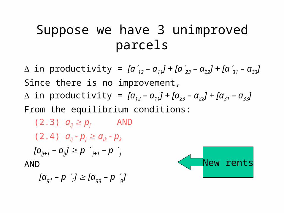
Suppose we have 3 unimproved parcels
in productivity = [a12 – a11] + [a23 – a22] + [a31 – a33]
Since there is no improvement,
in productivity = [a12 – a11] + [a23 – a22] + [a31 – a33]
From the equilibrium conditions:
(2.3) aij pj AND
(2.4) aij - pj aik - pk
[ajj+1 – ajj] p j+1 – p j
AND
[ag1 – p 1] [agg – p g]
New rents

Suppose we have 3 unimproved parcels
[ajj+1 – ajj] p j+1 – p j
AND
[ag1 – p 1] [agg – p g]
ALSO
[ajj+1 – ajj] p j+1 – p j
AND
[ag1 – p 1] [agg – p g]
New rents
Old rents
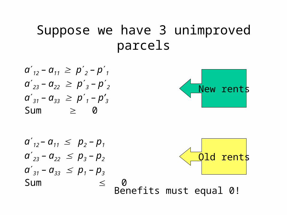
Suppose we have 3 unimproved parcels
a12 – a11 p2 – p1
a23 – a22 p3 – p2
a31 – a33 p1 – p’3
Sum 0
New rents
Old rents
a12 – a11 p2 – p1
a23 – a22 p3 – p2
a31 – a33 p1 – p3
Sum 0Benefits must equal 0!

Let’s improve a parcel (#1)
D = Benefits. Assume activity 1 moves to parcel 2, activity 2to parcel 3, etc.
1
111
)'()'(g
gggjjjj aaaaD
With no improvement on parcels 2 through g:
1
11
1
11
)()'(g
jjjj
g
jjjj aaaa
pj,aij
“Winning” aij changes;
Eq’m rent pj changes.
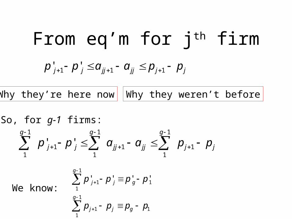
From eq’m for jth firm
jjjjjjjj ppaapp 111 ''
Why they’re here now Why they weren’t before
So, for g-1 firms:
jj
g
jjjj
g
jj
g
ppaapp
1
1
11
1
11
1
1
''
We know:
1
111
1
111 ''''
g
gjj
g
gjj
pppp
pppp

From eq’m for jth firm
)()'()''()'(
)'('')'(
)'(''
1111
1111
111
gggggggg
gggggggg
ggggg
ppaaDppaa
aappDppaa
ppaaDpp
Increased profit at new prices Increased profit at old prices
jjjjjjjj ppaapp 111 ''If we’re operating on the margin, we get equalities above:
)()'()''()'( 1111 gggggggg ppaaDppaa
1 1( ' )D p p
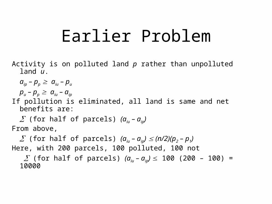
Earlier Problem
Activity is on polluted land p rather than unpolluted land u.
aip – pp aiu – pu
pu – pp aiu – aip
If pollution is eliminated, all land is same and net benefits are:
(for half of parcels) (aiu – aip)From above,
(for half of parcels) (aiu – aip) (n/2)(p2 – p1)Here, with 200 parcels, 100 polluted, 100 not
(for half of parcels) (aiu – aip) 100 (200 – 100) = 10000
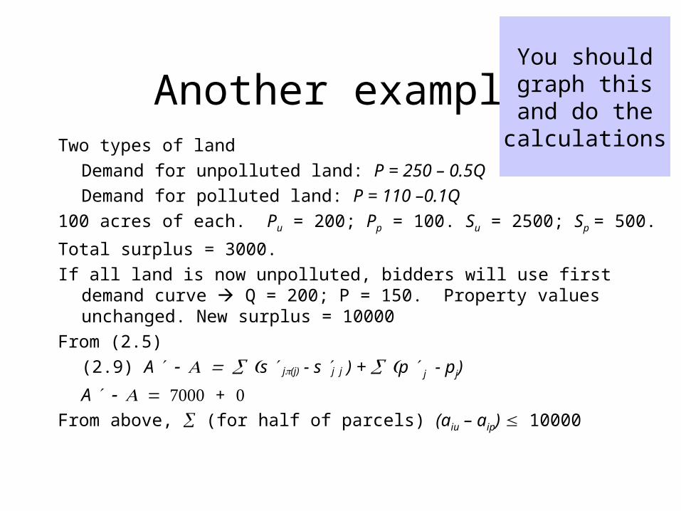
Another exampleTwo types of land
Demand for unpolluted land: P = 250 – 0.5Q
Demand for polluted land: P = 110 –0.1Q
100 acres of each. Pu = 200; Pp = 100. Su = 2500; Sp = 500.
Total surplus = 3000.
If all land is now unpolluted, bidders will use first demand curve Q = 200; P = 150. Property values unchanged. New surplus = 10000
From (2.5)
(2.9) A s j(j) - s jj ) + p j - pj)
A + From above, (for half of parcels) (aiu – aip) 10000
You shouldgraph thisand do the
calculations

Polinsky and Shavell
© Allen C. Goodman 2009
Polinsky and Shavell
Examine the distinction between closed and open cities when looking at the measurement of benefits.
Take a little different tack in the modeling but with similar results.
They use an indirect utility function:
V = V (y - T(k), p(k), a(k))
where k = distance, y = income, T = transportation costs, a(k) is an amenity.
We have V1 > 0, V2 < 0, V3 > 0. Why?
What can we do with this?
V = V (y - T(k), p(k), a(k))
Within a city dV = 0.
dV/dk = -V1T´ + V2p´ +V3 a´ = 0.
Leads to p´ = (V1/V2)T´- (V3/V2)a´.
(V1/V2) = [Utility/$]/[Utility/(acres/$)] (1/Land).
We have negative price-distance function.
With an open city V is fixed at V*, so suppose there is an increase in a(k).
For V to stay equal to V*, p(k) must rise.

What can we do with this?
Suppose we have a closed city.
V** = V (y - T(k), p(k), a(k))
V starts at V**. Suppose amenities increase everywhere but k. V** must rise.
Since amenities haven’t improved at k, p(k) must fall relative to elsewhere. This is an indirect effect.
Now increase a(k). p(k) must rise to maintain V**. This is the direct effect.

Regression analysis w/ PS
Cobb-Douglas Example
U = Axqa(k); + = 1.
x(k) = (y – T(k))
q(k) = (y – T(k))/p(k)
Putting x and q into U V(k) = C[y-T(k)]p(k)-a(k)C is a constant
Solve for p(k) as:
log p(k) = (1/) log (C/V*) + (1/) log [Y – T(k)] + () log a(k)
= b0 + b1 log [Y – T(k)] + b2 log a(k)

Regression analysis w/ PS
log p(k) = (1/) log (C/V*) + (1/) log [Y – T(k)] + () log a(k)
= b0 + b1 log [Y – T(k)] + b2 log a(k)In an open city, since V* is fixed, a change in a(k) will predict change in
log p(k).In closed city V* V**. Must know what happens to a(k) all over city.
Gen’l eq’m model is necessary.SO:
Changes in aggregate land values correspond to WTP only with an open city model.Eq’m rent schedule will give enough information to identify demand for a(k), all else equal; in “closed city” all else may not be equal.


