
Linear Algebra
and
DSP
Nuno Vasconcelos
UCSD

Vector spaces

Vector spaces
• Definition: a vector space is a set H where
– addition and scalar multiplication are defined and satisfy:
1) x+(x’+x’’) = (x+x’)+x” 5) x H
2) x+x’ = x’+x H 6) 1x = x
3) 0 H, 0 + x = x 7) ( ’ x) = ( ’)x
4) –x H, -x + x = 0 8) (x+x’) = x + x’
( scalar; x, x’, x” H ) 9) ( + ’)x = x + ’x
• the canonical example is Rd with standard
vector addition and scalar multiplication
e1
e2
ed
x
x’
x+x’
e2
e1
ed
x
x
Vector spaces
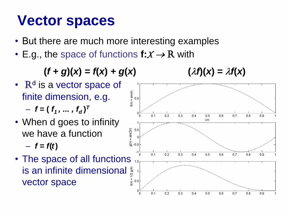
• But there are much more interesting examples
• E.g., the space of functions f:X R with
(f + g)(x) = f(x) + g(x) ( f)(x) = f(x)
• Rd is a vector space of
finite dimension, e.g.
– f = ( f1 , ... , fd )T
• When d goes to infinity
we have a function
– f = f (t )
• The space of all functions
is an infinite dimensional
vector space
Vector spaces
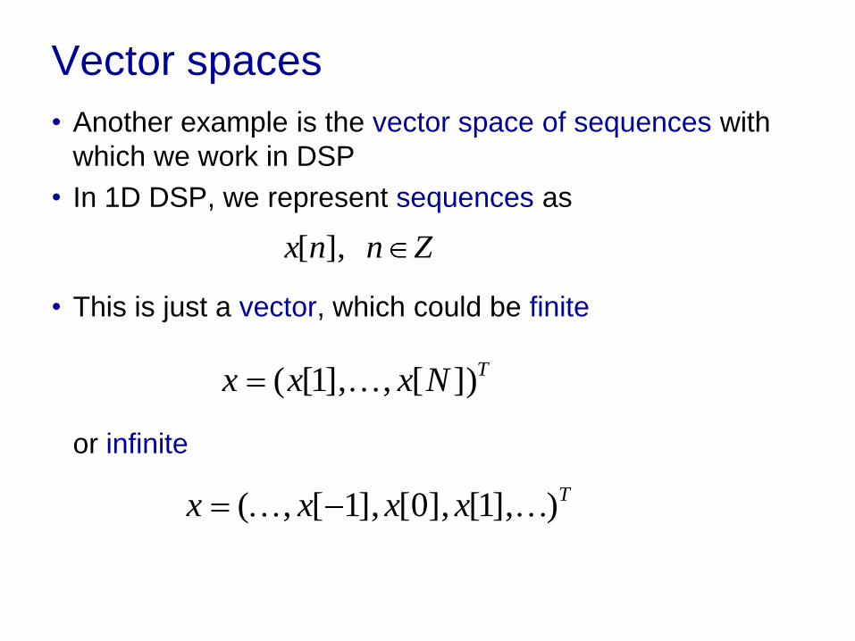
• Another example is the vector space of sequences with
which we work in DSP
• In 1D DSP, we represent sequences as
• This is just a vector, which could be finite
or infinite
Znnx ],[
TNxxx ])[,],1[(
Txxxx )],1[],0[],1[,(

• In this course we will talk a lot about sequences
• Sequences will always be represented in a vector space:
– A sequence is really just a point on such a space
– from above we know how to perform basic operations on points
– this is nice, because points can be quite abstract
– e.g. images:
an image is a function
on the image plane
it assigns a color f(x,y) to
each image
location (x,y)
the space of images
is a vector space (note: assumes
that images can be negative)
this image is a point in
Data Vector Spaces

• Because of this we can manipulate images by
manipulating their vector representations
• E.g., Suppose one wants to “morph” a(x,y) into b(x,y):
– One way to do this is via the path along the line from a to b.
c( ) = a + (b-a)
= (1- ) a + b
– for = 0 we have a
– for = 1 we have b
– for in (0,1) we have a point
on the line between a and b
• To morph images we can simply
apply this rule to their vector
representations!
Images
b
a
b-a
(b-a)

• When we make
c(x,y) = (1- ) a(x,y) + b(x,y)
we get “image morphing”:
• The point is that this is possible because the images are
points in a vector space.
Images
b
a
b-a
(b-a)
=0 =0.2 =0.4
=0.6 =0.8 =1
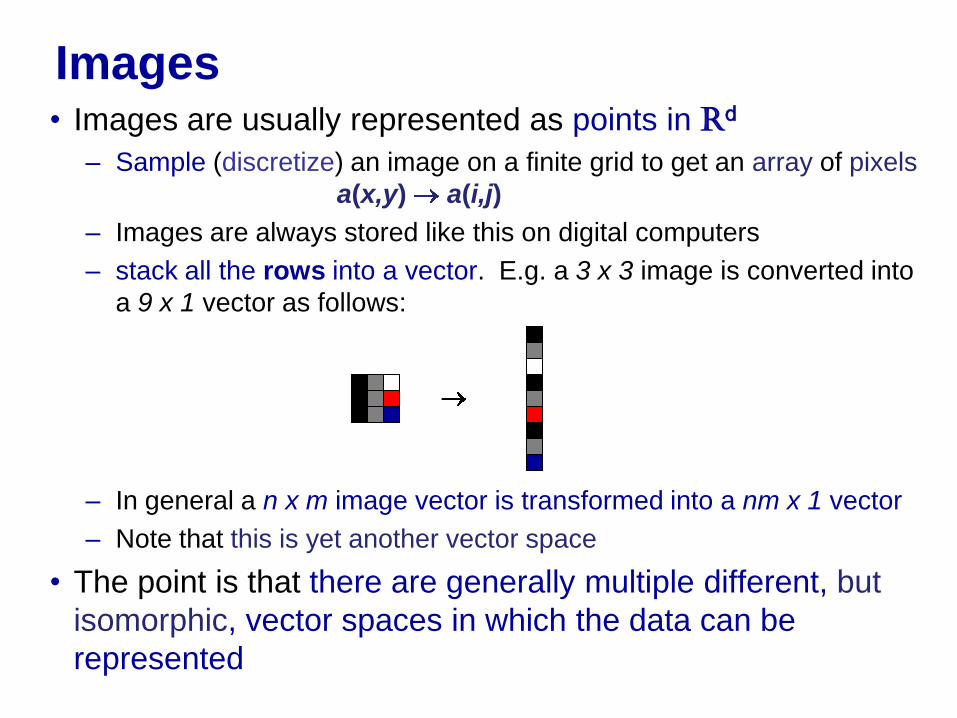
• Images are usually represented as points in Rd
– Sample (discretize) an image on a finite grid to get an array of pixels
a(x,y) a(i,j)
– Images are always stored like this on digital computers
– stack all the rows into a vector. E.g. a 3 x 3 image is converted into
a 9 x 1 vector as follows:
– In general a n x m image vector is transformed into a nm x 1 vector
– Note that this is yet another vector space
• The point is that there are generally multiple different, but
isomorphic, vector spaces in which the data can be
represented
Images

Text
• Another common type
of data is text
• Documents are
represented by
word counts:
– associate a counter
with each word
– slide a window through
the text
– whenever the word
occurs increment
its counter
• This is the way search
engines represent
web pages
Text
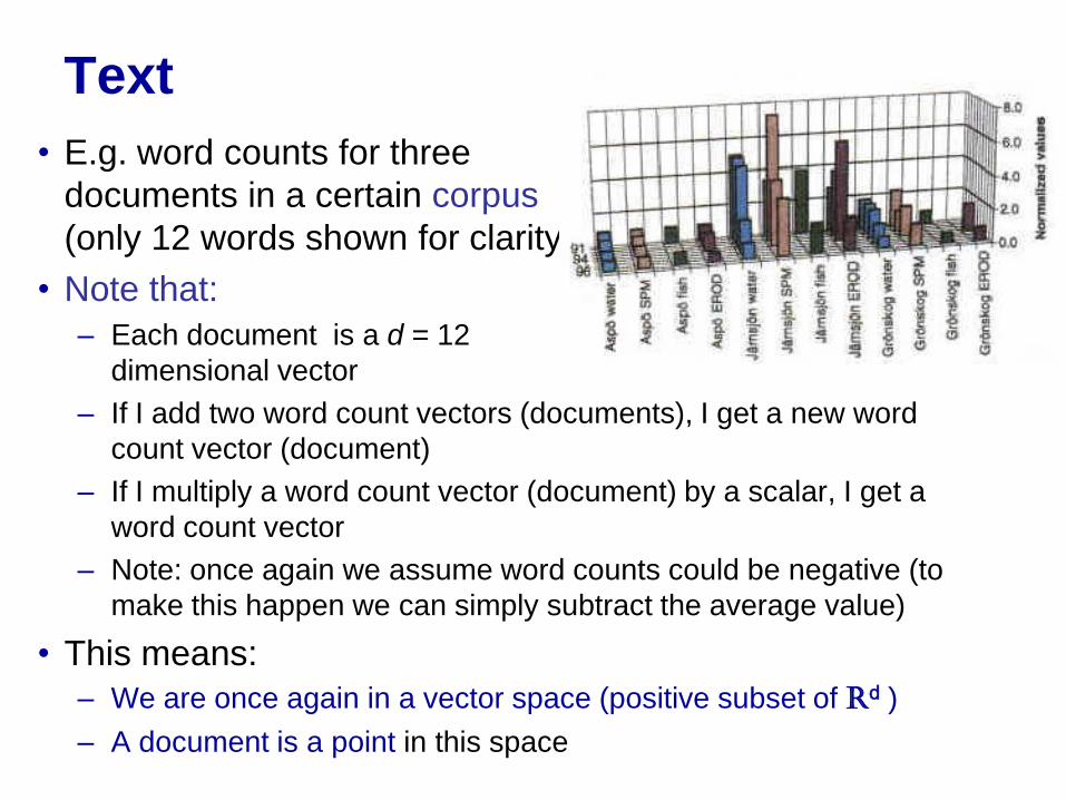
• E.g. word counts for three
documents in a certain corpus
(only 12 words shown for clarity)
• Note that:
– Each document is a d = 12
dimensional vector
– If I add two word count vectors (documents), I get a new word
count vector (document)
– If I multiply a word count vector (document) by a scalar, I get a
word count vector
– Note: once again we assume word counts could be negative (to
make this happen we can simply subtract the average value)
• This means:
– We are once again in a vector space (positive subset of Rd )
– A document is a point in this space

Dot-products and distances
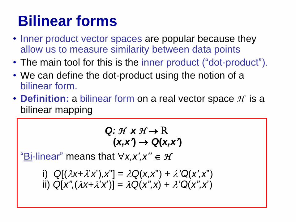
Bilinear forms • Inner product vector spaces are popular because they
allow us to measure similarity between data points
• The main tool for this is the inner product (“dot-product”).
• We can define the dot-product using the notion of a bilinear form.
• Definition: a bilinear form on a real vector space H is a bilinear mapping Q: H x H R (x,x’) Q(x,x’)
“Bi-linear” means that x,x’,x’’ H
i) Q[( x+ ’x’),x”] = Q(x,x”) + ’Q(x’,x”) ii) Q[x”,( x+ ’x’)] = Q(x”,x) + ’Q(x”,x’)
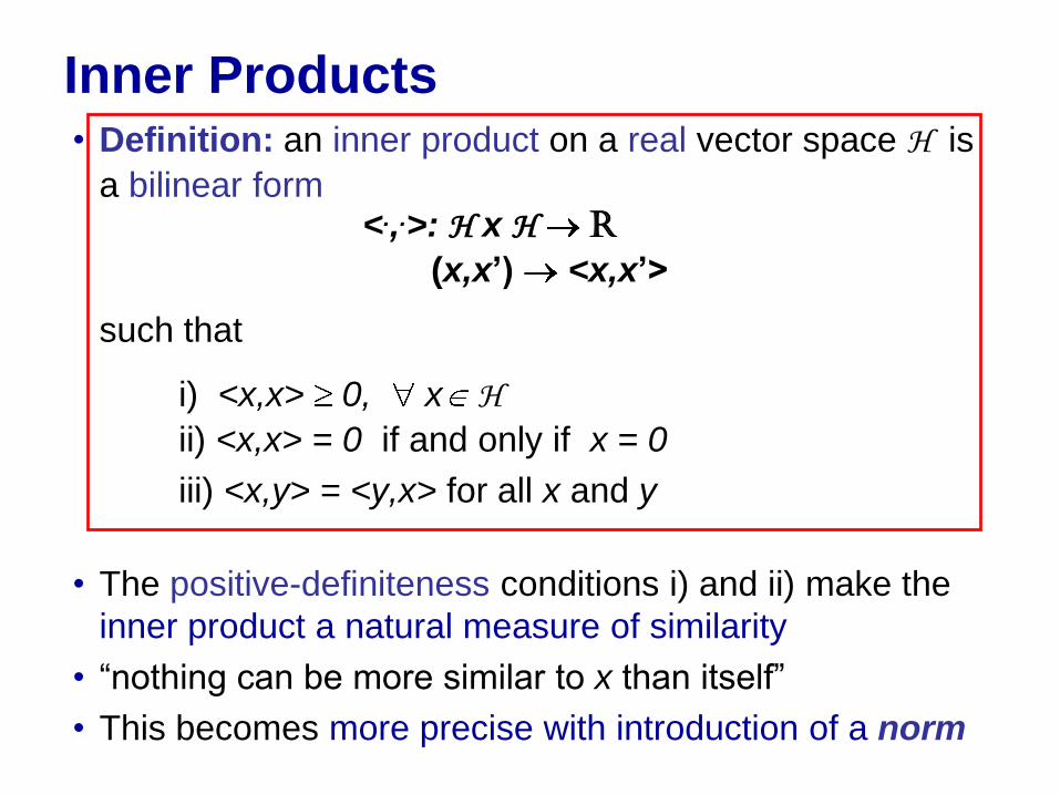
Inner Products • Definition: an inner product on a real vector space H is
a bilinear form <.,.>: H x H R
(x,x’) <x,x’>
such that
i) <x,x> 0, x H
ii) <x,x> = 0 if and only if x = 0
iii) <x,y> = <y,x> for all x and y
• The positive-definiteness conditions i) and ii) make the
inner product a natural measure of similarity
• “nothing can be more similar to x than itself”
• This becomes more precise with introduction of a norm
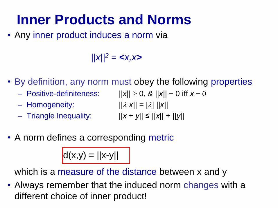
Inner Products and Norms • Any inner product induces a norm via
||x||2 = <x,x>
• By definition, any norm must obey the following properties
– Positive-definiteness: ||x|| 0, & ||x|| 0 iff x
– Homogeneity: || x|| = | | ||x||
– Triangle Inequality: ||x + y|| ≤ ||x|| + ||y||
• A norm defines a corresponding metric
d(x,y) = ||x-y||
which is a measure of the distance between x and y
• Always remember that the induced norm changes with a
different choice of inner product!

Inner Product
• Back to our examples:
– In Rd the standard inner product is
– Which leads to the standard Euclidean norm in Rd
– The distance between two vectors is the standard Euclidean distance in Rd
i
d
i
i
T yxyxyx1
,
d
i
i
T xxxx1
2
d
i
ii
T yxyxyxyxyxd1
2)()()(),(

Inner Product
• In signal processing these operations have special names:
– The inner product is the correlation between the two sequences
– The norm is the energy of the signal
– The Euclidean distance is the distance
i
d
i
i
T yxyxyx1
,
d
i
i
T xxxx1
2
d
i
ii
T yxyxyxyxyxd1
2)()()(),(

Inner Products and Norms • Note, e.g., that this immediately gives
a measure of similarity
between web pages
– compute word count vector xi
from page i, for all i
– distance between page i and
page j can be simply defined as:
– This allows us to find, in the web, the most similar page i to any given
page j.
• In fact, this is very close to the measure of similarity used by
most search engines!
• What about images and other continuous valued signals?
)()(),( ji
T
jijiji xxxxxxxxd
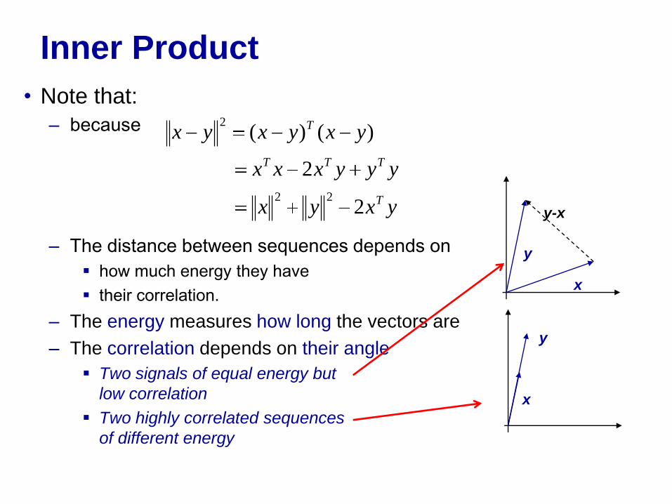
Inner Product
• Note that:
– because
– The distance between sequences depends on
how much energy they have
their correlation.
– The energy measures how long the vectors are
– The correlation depends on their angle
Two signals of equal energy but
low correlation
Two highly correlated sequences
of different energy
yxyx
yyyxxx
yxyxyx
T
TTT
T
2
2
)()(
22
2
y
x
y-x
y
x
Unit vectors
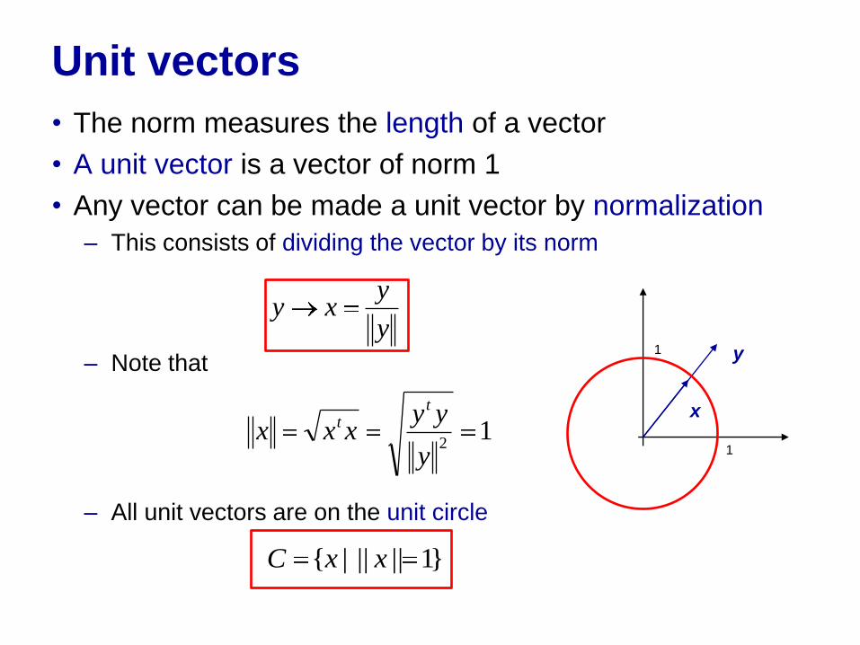
• The norm measures the length of a vector
• A unit vector is a vector of norm 1
• Any vector can be made a unit vector by normalization
– This consists of dividing the vector by its norm
– Note that
– All unit vectors are on the unit circle
y
yxy
y
x 1
2y
yyxxx
tt
}1|||| |{ xxC
1
1

Normalized correlation
• Is the correlation between normalized sequences
• And captures distance between them
• It can be shown that
y
y
x
x
yx
yxyx
TT
),(
y/||y||
x/||x||
),(22
222
2
yx
y
yy
yx
yx
x
xx
y
y
x
x TTT
),cos( yxyxyxT ),cos(),( yxyx
angle between x and y

Inner Products on Function Spaces
• Recall that the space of functions is an infinite
dimensional vector space
– The standard inner product is the natural extension of that in Rd
(just replace summations by integrals)
– The norm becomes the “energy” of the function
– The distance between functions the energy of the difference
between them
( ), ( ) ( ) ( )f x g x f x g x dx
2 2( ) ( )f x f x dx
2 2( ( ), ( )) ( ) ( ) [ ( ) ( )]d f x g x f x g x f x g x dx
Inner Products on Function Spaces
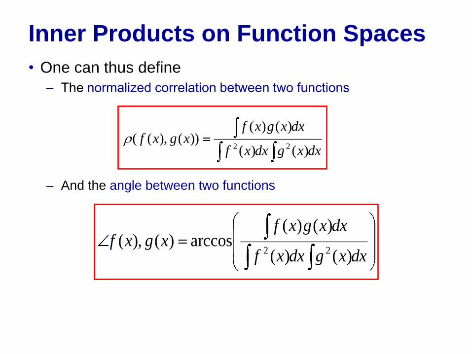
• One can thus define
– The normalized correlation between two functions
– And the angle between two functions
dxxgdxxf
dxxgxfxgxf
)()(
)()())(),((
22
dxxgdxxf
dxxgxfxgxf
)()(
)()(arccos)(),(
22

Bases
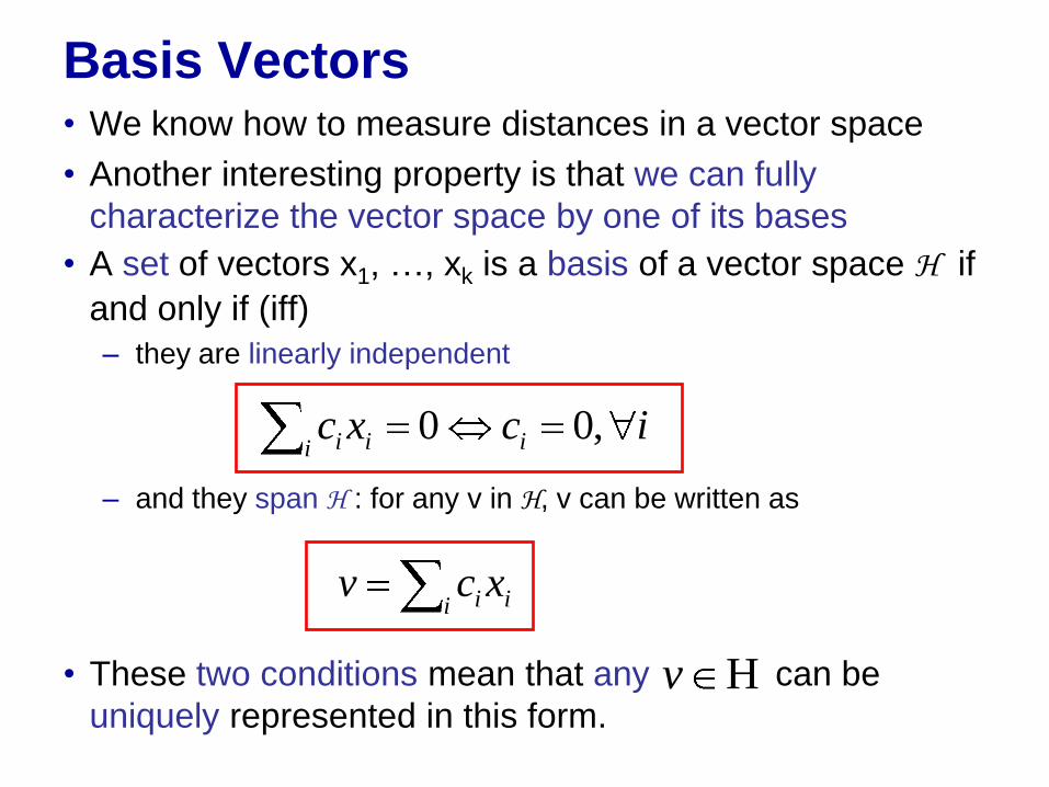
Basis Vectors • We know how to measure distances in a vector space
• Another interesting property is that we can fully
characterize the vector space by one of its bases
• A set of vectors x1, …, xk is a basis of a vector space H if
and only if (iff)
– they are linearly independent
– and they span H : for any v in H, v can be written as
• These two conditions mean that any can be
uniquely represented in this form.
i iii icxc ,00
i ii xcv
v H

Basis
• Note that
– By making the vectors xi the columns of a matrix X, these two
conditions can be compactly written as
– Condition 1. The vectors xi are linear independent:
– Condition 2. The vectors xi span H
• Also, all bases of H have the same number of vectors, which is called the dimension of H
– This is valid for any vector space!
00 cXc
0, 0 such that v c v Xc
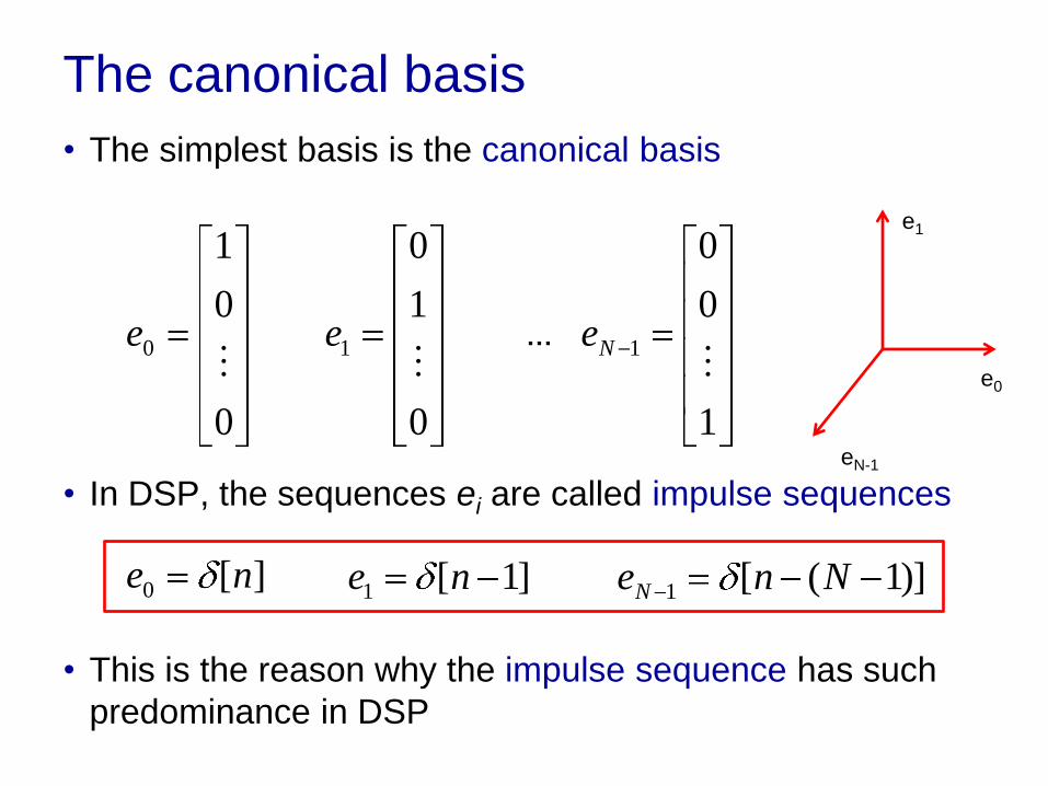
The canonical basis
• The simplest basis is the canonical basis
• In DSP, the sequences ei are called impulse sequences
• This is the reason why the impulse sequence has such
predominance in DSP
0
0
1
0
e
0
1
0
1
e
1
0
0
1
Ne…
e0
e1
eN-1
][0 ne ]1[1 ne )]1([1 NneN
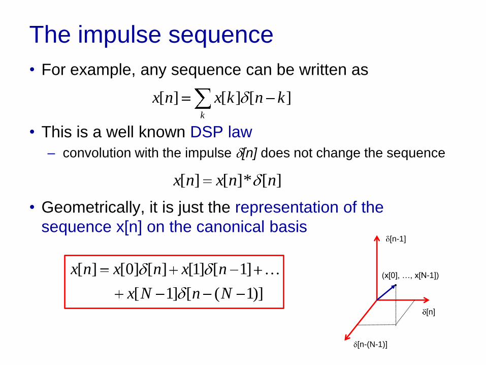
The impulse sequence
• For example, any sequence can be written as
• This is a well known DSP law
– convolution with the impulse [n] does not change the sequence
• Geometrically, it is just the representation of the
sequence x[n] on the canonical basis
k
knkxnx ][][][
[n]
[n-1]
[n-(N-1)]
. (x[0], …, x[N-1])
][*][][ nnxnx
)]1([]1[
]1[]1[][]0[][
NnNx
nxnxnx

The impulse sequence
• Has unit norm
• And is orthogonal to the other impulse sequences
– For any l, m not equal
– Hence
– E.g.
1][][ 2
k
kn
1][][][],[ mklkmnlnk
2][],[ mnln
Tn )0,...,0,1,0(]1[
Tn )0,...,1,0,0(]2[Orthogonal
sequences
[n]
[n-1]
[n-(N-1)]
. (x[0], …, x[N-1])
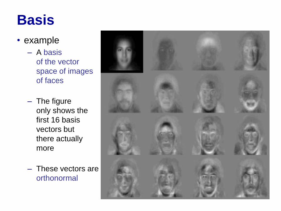
Basis
• example
– A basis
of the vector
space of images
of faces
– The figure
only shows the
first 16 basis
vectors but
there actually
more
– These vectors are
orthonormal

Orthogonality
• Two vectors are orthogonal iff their inner product is zero
– e.g.
in the space of functions defined on [0,2 ], cos(ax) and sin(ax)
are orthogonal
• Two subspaces V and W are orthogonal, V W, if
every vector in V is orthogonal to every vector in W
• a set of vectors x1, …, xk is called
– orthogonal if all pairs of vectors are orthogonal.
– orthonormal if all vectors also have unit norm.
22 2
0 0
sinsin( )cos( ) 0
2
axax ax dx
a
ji
jixx ji
if ,1
if ,0,
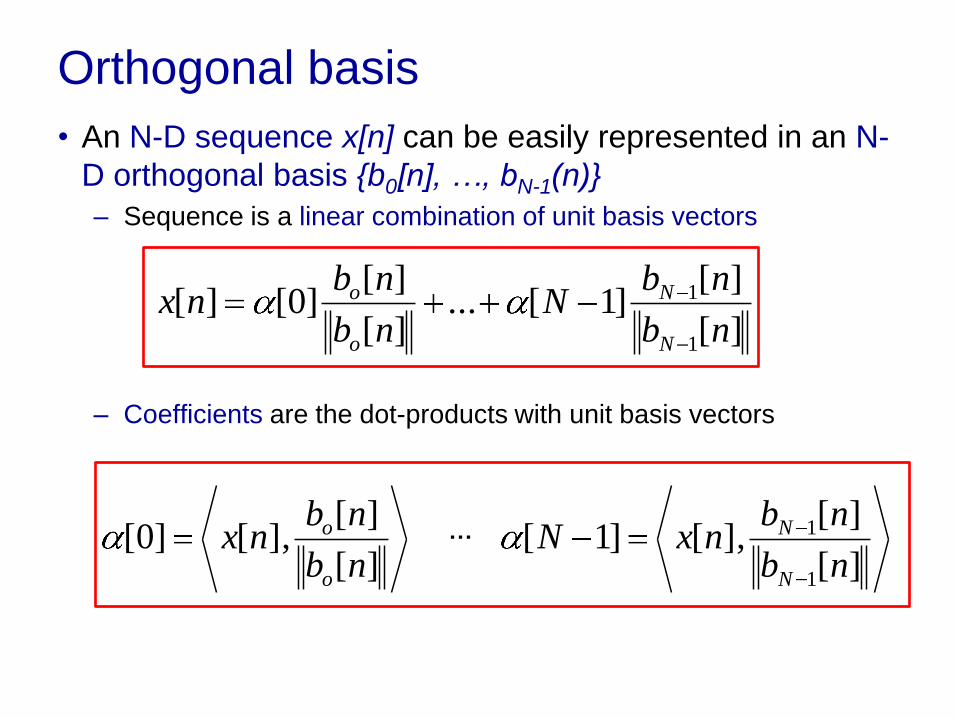
Orthogonal basis
• An N-D sequence x[n] can be easily represented in an N-
D orthogonal basis {b0[n], …, bN-1(n)}
– Sequence is a linear combination of unit basis vectors
– Coefficients are the dot-products with unit basis vectors
][
][]1[...
][
][]0[][
1
1
nb
nbN
nb
nbnx
N
N
o
o
][
][],[]0[
nb
nbnx
o
o
][
][],[]1[
1
1
nb
nbnxN
N
N…

Orthogonal basis
• Note that for the impulse basis, bm[n] = [n-m]
– The basis vectors are already unit vectors
– The sequence is
– The coefficients are
– And we are back to the fundamental formula
k
1
][][
)]1([]1[...][]0[
][]1[...][]0[][
knk
NnNn
nbNnbnx No
][][],[][],[][ kxknnxnbnxk k
k
knkxnx ][][][

Matrices and LTI systems

Matrix
• an m x n matrix represents a linear operator that maps a vector from the domain X = Rn to a vector in the codomain Y = Rm
• E.g. the equation y = Ax
sends x in Rn to y in Rm
according to
X Y
• note that there is nothing magical about this, it follows rather
mechanically from the definition of matrix-vector multiplication
nmnm
n
m x
x
aa
aa
y
y
1
1
1111
e1
e2
en
x
e1
em
y A

Linear systems
• Hence, a square matrix can be used to represent a linear
system
• domain X = RN is the vector space of input sequences
• codomain Y = RN is the vector space of output sequences
• Note that if the input is a linear combination of sequences
• The output is the same linear combination of the
corresponding outputs
• This is the definition of linear system
][][][ 21 nbxnaxnx
][][][][
][][
2121
21
nbynaynbAxnaAx
[n])bx[n]A(axnAxny

Matrix-Vector Multiplication I
• Consider y = Ax, i.e. yi = j=1n aijxj
• We can think of this as
• where “(– ai –)” means the ith row of A. Hence
– the ith component of y is the inner product of (– ai –) and x.
– y is the projection of x on the subspace (of the domain space) spanned
by the rows of A
1
1
1
n
i i in ij j i
j
n
x
y a a a x a x
x
e1
e2
en
x A’s action in X
-am-
-a1-
x
y1
ym
-a2-
y2
, i = 1,…,m
(m rows)
X X

Matrix-Vector Multiplication II
• But there is more. Let y = Ax, i.e. yi = j=1n aijxj , now be written as
• where ai with “|” above and below means the ith column of A.
• hence
– xi is the ith component of y in the subspace (of the co-domain) spanned
by the columns of A
– y is a linear combination of the columns of A
nn
nmnm
nnn
j
jij
m
xaxa
xaxa
xaxa
xa
y
y
|
|
|
|
11
11
1111
1
1
e1
e2
en
x
A maps from X to Y
|
an
|
y
x1 |
a1
|
xn
X Y

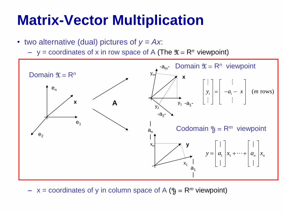
Matrix-Vector Multiplication
• two alternative (dual) pictures of y = Ax:
– y = coordinates of x in row space of A (The X = Rn viewpoint)
– x = coordinates of y in column space of A (Y = Rm viewpoint)
e1
e2
en
x A
-am-
-a1-
x
y1
ym
-a2-
y2
|
an
|
y
x1 |
a1
|
xn
( rows)i i my a x
1 1
| |
| |
n ny a x a x
Domain X = Rn
Domain X = Rn viewpoint
Codomain Y = Rm viewpoint

A cool trick
• the matrix multiplication formula
also applies to “block matrices” when these are defined
properly
• for example, if A,B,C,D,E,F,G,H are matrices,
• only but important caveat: the sizes of A,B,C,D,E,F,G,H
have to be such that the intermediate operations make
sense! (they have to be “conformal”)
k
kjikij bacABC
A B E F AE BG AF BH
C D G H CE DG CF DH

Matrix-Vector Multiplication
• This makes it easy to derive the two alternative pictures
• The row space picture (or viewpoint):
is just like scalar multiplication, with blocks (–ai-) and x
• The column space picture (or viewpoint):
is just a inner product, with (scalar) blocks xi and the
column blocks of A.
xaxa
x
x
aay inxxni
n
inini )()( 11
1
i
ii
xn
x
mxmx
n
n
inini xa
x
x
aa
x
x
aay
|
|
)(
)(
||
||
11
111
11
1
1
Matrix-Vector Multiplication
• two alternative (dual) pictures of y = Ax:
– y = coordinates of x in row space of A (The X = Rn viewpoint)
– x = coordinates of y in column space of A (Y = Rm viewpoint)
e1
e2
en
x A
-am-
-a1-
x
y1
ym
-a2-
y2
|
an
|
y
x1 |
a1
|
xn
( rows)i i my a x
1 1
| |
| |
n ny a x a x
Domain X = Rn
Domain X = Rn viewpoint
Codomain Y = Rm viewpoint

Square n x n matrices
• in this case m = n and the row and column subspaces are
both equal to (copies of) Rn
e1
e2
en
x A
-an-
-a1-
x
y1
yn
-a2-
y2
|
an
|
y
x1 |
a1
|
xn
|
a2
|
x2

LTI systems
• A is time invariant when
– x[n] has response y[n]
– If and only if, for any m, x[n-m] has response y[n-m]
– How does this constrain A?
Let x[n] = [n]
call the output impulse response
Using the codomain viewpoint
][][][][ mnAxmnynAxny
][][ nAnh
|
|
0
|
|
0
|
|
1
|
|
][ 1121 aaaanh N
|
an
|
y
x1 |
a1
|
xn
1 1
| |
| |
n ny a x a x
“Impulse response is first column of A”
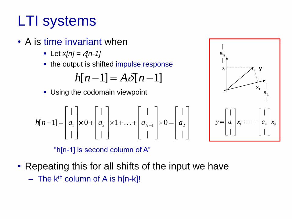
LTI systems
• A is time invariant when Let x[n] = [n-1]
the output is shifted impulse response
Using the codomain viewpoint
• Repeating this for all shifts of the input we have
– The kth column of A is h[n-k]!
]1[]1[ nAnh
|
|
0
|
|
1
|
|
0
|
|
]1[ 2121 aaaanh N
|
an
|
y
x1 |
a1
|
xn
1 1
| |
| |
n ny a x a x
“h[n-1] is second column of A”

LTI systems
• The matrix A has the structure
• Columns are shifts of the impulse response
– Check:
– what if impulse response is the impulse?
– A is the identity matrix
– Ax = x for all x
– The system does not change
the input
– It is an all-pass filter
|||
)]1([ ]1[ ][
|||
NnhnhnhA
100
010
001
A

LTI systems
• What are the rows?
– Note that we can write
– the kth row of Ax is
– This is the sequence
– Obtained by flipping h and shifting by k
]0[]2[]1[
]2[]0[]1[
]1[]1[]0[
hNhNh
Nhhh
Nhhh
A
])1([]1[][[ Nkhkhkh
][][ nkhngk
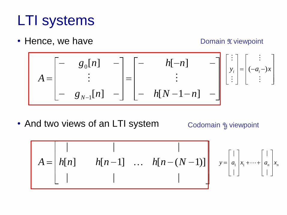
LTI systems
• Hence, we have
• And two views of an LTI system
]1[
][
][
][
1
0
nNh
nh
ng
ng
A
N
|||
)]1([ ]1[ ][
|||
NnhnhnhA 1 1
| |
| |
n ny a x a x
Domain X viewpoint
Codomain Y viewpoint
xay ii )(

Convolution
• Two ways to compute the output
• Under the domain viewpoint
• We obtain the convolution formula
-am-
-a1-
x
y1
ym
-a2-
y2
( rows)i i my a x
Domain X viewpoint
][],1[
][],[
][
]1[
][
]1[
]0[
nxnNh
nxnh
nx
nNh
nh
Ny
y
n
nxnkhnxnkhky ][][][],[][

Convolution
• Under the codomain viewpoint
• We obtain the alternative view of
convolution
• Note that the formulas are the same, but interpretation is
different
Codomain X viewpoint
k
kxknhny ][][][
]1[
|
)]1([
|
]0[
|
][
|
|
][
|
|||
)]1([ ]1[ ][
|||
|
][
|
NxNnhxnh
nxNnhnhnhny
1 1
| |
| |
n ny a x a x
|
an
|
y
x1 |
a1
|
xn

Example
• Impulse response:
• Input:
• System:
n
h[n]
n
x[n]
a b c
d e
A
Domain viewpoint
A
Codomain viewpoint
,
,
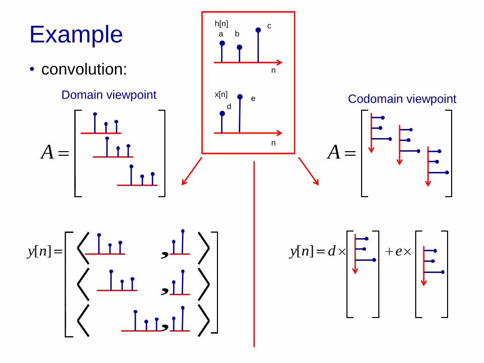
Example
• convolution:
A
Domain viewpoint
A
Codomain viewpoint
n
h[n]
n
x[n]
a b c
d e
,][ny edny ][

The fundamental spaces
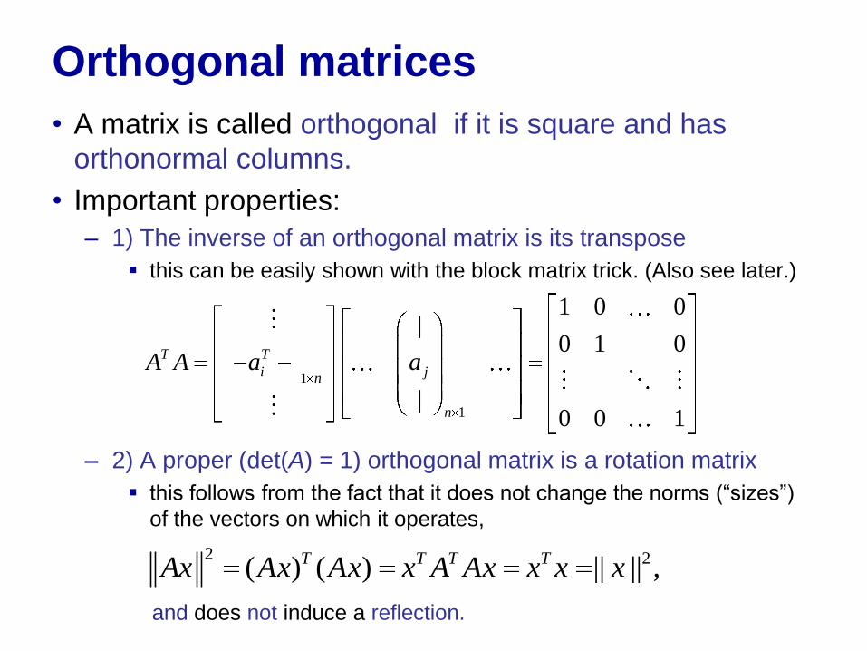
Orthogonal matrices
• A matrix is called orthogonal if it is square and has
orthonormal columns.
• Important properties:
– 1) The inverse of an orthogonal matrix is its transpose
this can be easily shown with the block matrix trick. (Also see later.)
– 2) A proper (det(A) = 1) orthogonal matrix is a rotation matrix
this follows from the fact that it does not change the norms (“sizes”)
of the vectors on which it operates,
and does not induce a reflection.
1
1
1 0 0|
0 1 0
|0 0 1
T T
i jn
n
A A a a
2 2( ) ( ) || || ,T T T TAx Ax Ax x A Ax x x x

Rotation matrices
• The combination of
1. “operator” interpretation
2. “block matrix trick”
is useful in many situations
• Poll:
– “What is the matrix R that rotates the plane R2 by degrees?”
e1
e2
Rotation matrices
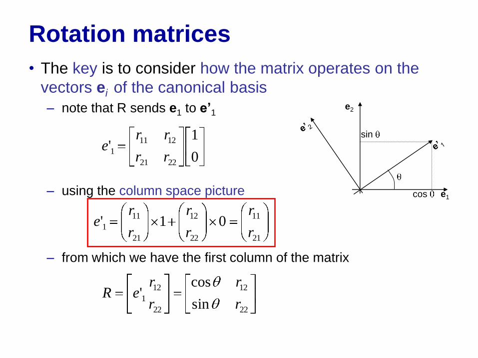
• The key is to consider how the matrix operates on the
vectors ei of the canonical basis
– note that R sends e1 to e’1
– using the column space picture
– from which we have the first column of the matrix
0
1'
2221
1211
1rr
rre
21
11
22
12
21
11
1 01'r
r
r
r
r
re
e1
e2
cos
sin
22
12
22
12
1sin
cos'
r
r
r
reR
Rotation Matrices
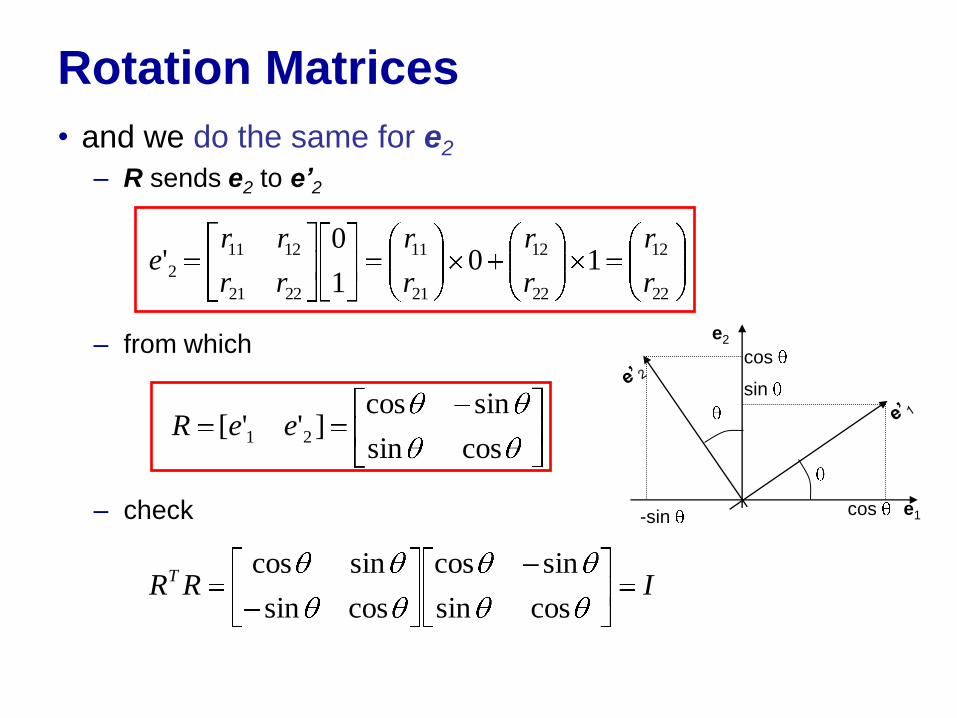
• and we do the same for e2
– R sends e2 to e’2
– from which
– check e1
e2
cos
sin
cos
-sin
22
12
22
12
21
11
2221
1211
2 101
0'
r
r
r
r
r
r
rr
rre
cossin
sincos]''[ 21 eeR
IRRT
cossin
sincos
cossin
sincos
Analysis/synthesis
• one interesting case is that of matrices with orthogonal
columns
• note that, in this case, the columns of A are
– a basis of the column space of A
– a basis of the row space of AT
• this leads to an interesting interpretation of the two
pictures
– consider the projection of x into the row space of AT
y = AT x
– due to orthonormality, x can then be synthesized by using the
column space picture
x’ = A y
Analysis/synthesis
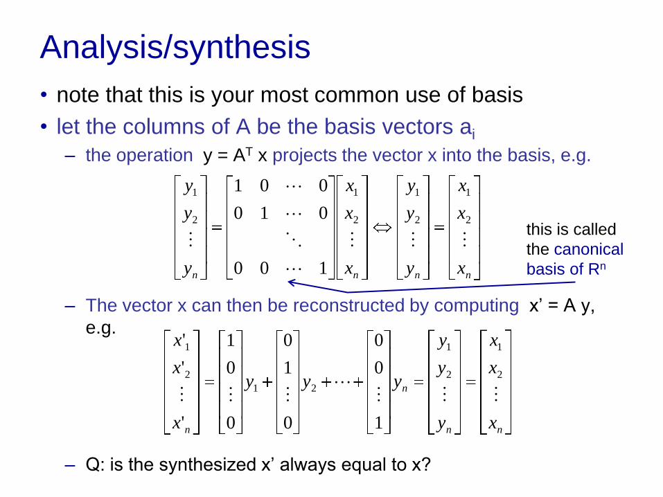
• note that this is your most common use of basis
• let the columns of A be the basis vectors ai
– the operation y = AT x projects the vector x into the basis, e.g.
– The vector x can then be reconstructed by computing x’ = A y,
e.g.
– Q: is the synthesized x’ always equal to x?
nnnn x
x
x
y
y
y
x
x
x
y
y
y
2
1
2
1
2
1
2
1
100
010
001
nn
n
n x
x
x
y
y
y
yyy
x
x
x
2
1
2
1
21
2
1
1
0
0
0
1
0
0
0
1
'
'
'
this is called
the canonical
basis of Rn
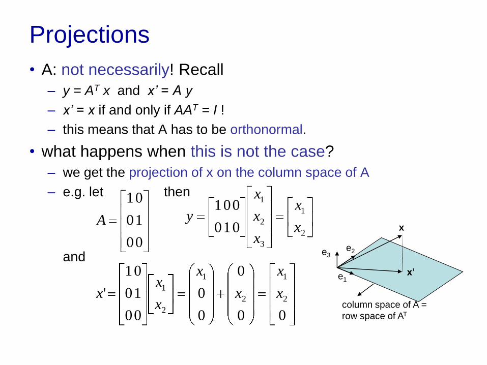
Projections
• A: not necessarily! Recall
– y = AT x and x’ = A y
– x’ = x if and only if AAT = I !
– this means that A has to be orthonormal.
• what happens when this is not the case?
– we get the projection of x on the column space of A
– e.g. let then
and 0
1
0
0
0
1
A2
1
3
2
1
0
0
1
0
0
1
x
x
x
x
x
y
00
0
0
0
0
1
0
0
0
1
' 2
1
2
1
2
1x
x
x
x
x
xx
e1
e2 e3
x
x’
column space of A =
row space of AT
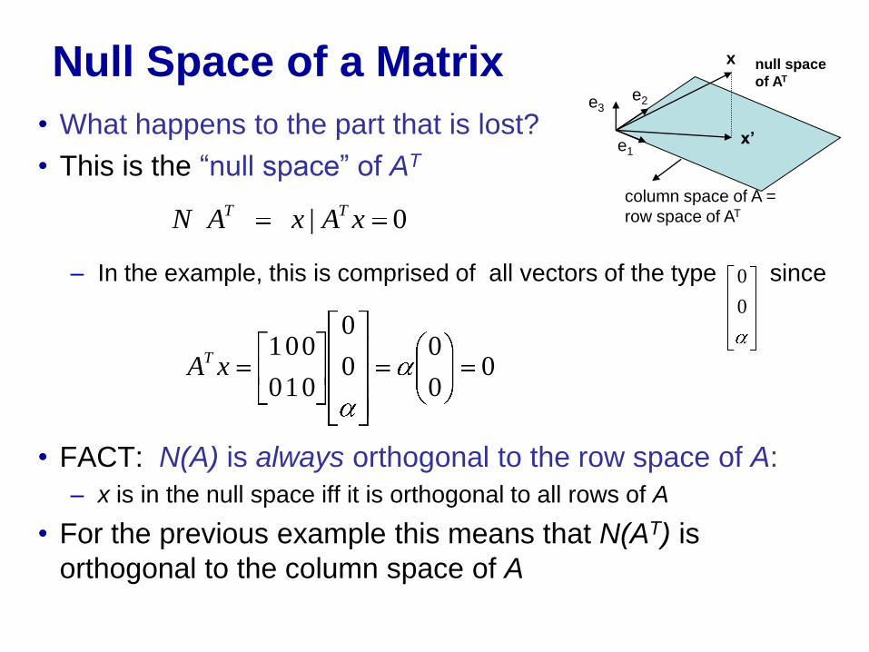
Null Space of a Matrix
• What happens to the part that is lost?
• This is the “null space” of AT
– In the example, this is comprised of all vectors of the type since
• FACT: N(A) is always orthogonal to the row space of A:
– x is in the null space iff it is orthogonal to all rows of A
• For the previous example this means that N(AT) is
orthogonal to the column space of A
| 0T TN A x A x
0
0
00
00
0
0
0
1
0
0
1xAT
e1
e2 e3
x
x’
column space of A =
row space of AT
null space
of AT

Orthonormal matrices
• Q: why is the orthonormal case special?
• because here there is no null space of AT
• recall that for all x in N(AT)
–
• the only vector in the null space is 0
• this makes sense:
– A has n orthonormal columns, e.g.
– these span all of Rn
– there is no extra room for an orthogonal space
– the null space of AT has to be empty
– the projection into row space of AT (=column space of A) is the
vector x itself
• in this case, we say that the matrix has full rank
000 AxxAT
100
010
001
A
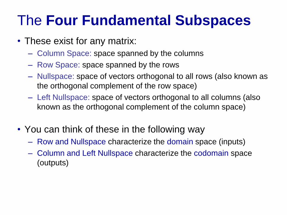
The Four Fundamental Subspaces
• These exist for any matrix:
– Column Space: space spanned by the columns
– Row Space: space spanned by the rows
– Nullspace: space of vectors orthogonal to all rows (also known as
the orthogonal complement of the row space)
– Left Nullspace: space of vectors orthogonal to all columns (also
known as the orthogonal complement of the column space)
• You can think of these in the following way
– Row and Nullspace characterize the domain space (inputs)
– Column and Left Nullspace characterize the codomain space
(outputs)

• Domain X = Rn
– y = coordinates of x in row space of A
– Row space: space of “useful inputs”,
which A maps to non-zero output
– Null space: space of “useless inputs”,
mapped to zero
– Operation of a matrix on its domain X = Rn
– Q: what is the null space of a low-pass filter?
Domain viewpoint
e1
e2
en
x A
( rows)i i my a x
-am-
-a1-
x
y1
ym
}0|{)( AxxAN
Null
space

• Codomain Y = Rm
– x = coordinates of y in column space of A
– Column space: space of “possible outputs”,
which A can reach
– Left Null space: space of “impossible
outputs”, cannot be reached
– Operation of a matrix on its codomain Y = Rm
– Q: what is the column space of a low-pass filter?
Codomain viewpoint
e1
e2
en
x A
}0|{)( AyyAL T
Left Null
space
1 1
| |
| |
n ny a x a x
|
an
| y
x1 |
a1
|
xn
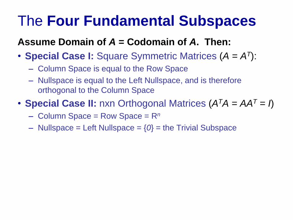
The Four Fundamental Subspaces
Assume Domain of A = Codomain of A. Then:
• Special Case I: Square Symmetric Matrices (A = AT):
– Column Space is equal to the Row Space
– Nullspace is equal to the Left Nullspace, and is therefore
orthogonal to the Column Space
• Special Case II: nxn Orthogonal Matrices (ATA = AAT = I)
– Column Space = Row Space = Rn
– Nullspace = Left Nullspace = {0} = the Trivial Subspace

Linear systems as matrices
• A linear and time invariant system
– of impulse response h[n]
– responds to signal x[n] with output
– this is the convolution of x[n] with h[n]
• The system is characterized by a matrix
– note that
– the output is the projection of the input on the space spanned by
the functions gn[k]
k
nn knhkgkgkxny ][][ with ],[][][
][
]2[
]1[
]0[]2[]1[
)]2([]0[]1[
)]1([]1[]0[
][
]2[
]1[
2
1
nx
x
x
hnhnh
nhhh
nhhh
x
g
g
g
ny
y
y
n
k
knhkxny ][][][

Linear systems as matrices
• the matrix
– characterizes the response of the system to any input
– the system projects the input into shifted and flipped copies of its
impulse response h[n]
– note that the column space is the space spanned by the vectors
h[n], h[n-1], …
– this is the reason why the impulse response determines the
output of the system
– e.g. a low-pass filter is a filter such that the column space of A
only contains low-pass low pass signals
– e.g. if h[n] is the delta function, A is the identity
]0[]2[]1[
)]2([]0[]1[
)]1([]1[]0[
hnhnh
nhhh
nhhh
A


![A DSP-Based Space Vector Modulation Direct Torque …journal.esrgroups.org/jes/papers/5_3_4.pdf · complex. In [10, 11], discrete space vector modulation DTC approach is used to reduce](https://cdn.vdocument.in/doc/165x107/5a953d657f8b9adb5c8c5e69/a-dsp-based-space-vector-modulation-direct-torque-in-10-11-discrete-space.jpg)


