IN THE FIELD OF TECHNOLOGYDEGREE PROJECT INDUSTRIAL ENGINEERING AND MANAGEMENTAND THE MAIN FIELD OF STUDYINDUSTRIAL MANAGEMENT,SECOND CYCLE, 30 CREDITS
, STOCKHOLM SWEDEN 2017
Liquidity risk in real estate investmentsfrom a perspective of institutional investors
MARIA HÄGGBOM
KARIN ÅSENIUS
KTH ROYAL INSTITUTE OF TECHNOLOGYSCHOOL OF INDUSTRIAL ENGINEERING AND MANAGEMENT

Liquidity risk in real estate investments from a perspective of institutional investors
by
Maria Häggbom Karin Åsenius
Master of Science Thesis INDEK 2017:22
KTH Industrial Engineering and Management
Industrial Management
SE-100 44 STOCKHOLM

Likviditetsrisk i fastighetsinvesteringar från institutionella investerares perspektiv
av
Maria Häggbom Karin Åsenius
Examensarbete INDEK 2017:22
KTH Industriell teknik och management
Industriell ekonomi och organisation
SE-100 44 STOCKHOLM
Master of Science Thesis INDEK 2017:22
Liquidity risk in real estate investments from a perspective of institutional investors
Maria Häggbom
Karin Åsenius
Approved
2017-05-31
Examiner
Anders Broström
Supervisor
Christian Thomann
Commissioner
SEB
Contact person
Mikael Anveden
Abstract
Over the last couple of years interest rates have decreased. This has led institutional investors to search for alternative assets which generate return. One of the assets which has gained attention in the light of this change is real estate. Historically real estate has presented a high risk adjusted return and since 2006 house prices in Sweden has increased by a total of 56% [Carlgren, 2016]. Real estate is an illiquid asset and it can take time to sell a real estate asset at a price agreed on by both parts. In this study the implications for institutional investors of including or increasing the allocation towards illiquid assets are investigated from a portfolio perspective. In addition, other risk factors relevant to real estate investments are examined together with how the specific liquidity risks can be identified and measured.
The research is divided into two parts. One qualitative part consisting of interviews with investors of Swedish pension funds to understand their view on real estate investments. The other part is quantitative and consists of different ways to model and calculate risks associated with liquidity. The modeling includes ex-ante variance scaling, de-smoothing, scenarios of forced sales and liquidation premium.
The results show that the interview participants' perception of liquidity risk is larger than that obtained through quantitative risk measures. The outstanding performance of real estate seen in indexes may rather be an effect of artificial smoothing1 rather than the performance in the asset class. A scenario which could impact the investors with regards to illiquid assets is the risk of forced sale. However the situation with strong balance sheets for many of the Swedish institutional investors decrease this risk. The total portfolio risk from illiquid assets are also limited as an effect of the limited allocation to these asset classes.
Key-words Real estate, Institutional investors, Measuring risk, Illiquidity
1 Artificial smoothing - Smoothing of peak and low historical transaction value due to inherent limitations in
the valuation process

Examensarbete INDEK 2017:22
Likviditetsrisk i fastighetsinvesteringar från institutionella investerares perspektiv
Maria Häggbom
Karin Åsenius
Godkänt
2017-05-31
Examinator
Anders Broström
Handledare
Christian Thomann
Uppdragsgivare
SEB
Kontaktperson
Mikael Anveden
Sammanfattning
Under de senaste åren har räntorna sjunkit. Detta har lett till att institutionella investerare söker efter alternativa investeringsalternativ som kan generera avkastning trots låga räntenivåer. En av de tillgångar som har fått uppmärksamhet till följd av denna förändring är fastigheter. Historiskt har fastigheter genererat en hög risk justerad avkastning och sedan 2006 har bostadspriser i Sverige ökat med 56% [Carlgren, 2016]. Fastigheter är en illikvid tillgång och det kan ta tid att sälja en fastighetstillgång till ett pris som båda parterna kan komma överens om. I denna studie har följderna av institutionella investerare och deras allokering till illikvida tillgångar ifrån ett portföljperspektiv undersökts. Utöver detta har även andra riskfaktorer som är relevanta för fastighetsinvesteringar studerats tillsammans med hur specifika likviditetsrisker kan identifieras och mätas.
Studien är uppdelad i två delar. En kvalitativ del bestående av intervjuer med investerare i svenska pensionsfonder för att få en förståelse för deras syn på fastighetsinvesteringar. Den andra, kvantitativa delen, består av olika metoder för att modellera och beräkna risker som kan associeras med likviditet. Modelleringen inkluderar ex-ante varians skalning, de-smoothing, scenarioanalys vid tvingad försäljning och likvideringspremie.
Resultaten visar att intervjudeltagarnas uppfattning av likviditetsrisk är högre än den som tagits fram från kvantitativa riskmått. Det iögonfallande historiska riskjusterade avkastningen som kan ses från fastighetsindex kan också vara en effekt av artificiell smoothing2 istället för faktisk hög riskjusterad avkastning från det underliggande. Ett scenario som kan påverka investerarna med tanke på illikvida tillgångar är risken för tvingad försäljning. I dagsläget har dock svenska institutionella investerare starka balansräkningar vilket minskar risken för tvingad försäljning. Den totala risken från illikvida tillgångar i portföljen påverkas också av att de flesta investerare har en begränsad andel av sina portföljer allokerade till illikvida tillgångar.
Nyckelord Fastigheter, Institutionella investerare, Risk mått, Illikviditet
2 Artificiell smoothing – Utjämning av toppar och dalar i historiska transaktionspriser till följd av
begränsningar inbyggda i värderingsprocessen

Contents
1 Introduction 11.1 Background . . . . . . . . . . . . . . . . . . . . . . . . . . . . . . . . . . . 1
1.2 Problematization . . . . . . . . . . . . . . . . . . . . . . . . . . . . . . . . 2
1.3 Purpose and research questions . . . . . . . . . . . . . . . . . . . . . . . . 3
1.4 Limitations . . . . . . . . . . . . . . . . . . . . . . . . . . . . . . . . . . . 3
1.5 The study’s contribution . . . . . . . . . . . . . . . . . . . . . . . . . . . . 4
2 Method 62.1 Research design . . . . . . . . . . . . . . . . . . . . . . . . . . . . . . . . . 6
2.2 Research process . . . . . . . . . . . . . . . . . . . . . . . . . . . . . . . . 6
2.3 Literature review . . . . . . . . . . . . . . . . . . . . . . . . . . . . . . . . 7
2.4 Interviews . . . . . . . . . . . . . . . . . . . . . . . . . . . . . . . . . . . . 7
2.4.1 Interview selection . . . . . . . . . . . . . . . . . . . . . . . . . . . 8
2.4.2 Structure . . . . . . . . . . . . . . . . . . . . . . . . . . . . . . . . 9
2.4.3 Ethical considerations . . . . . . . . . . . . . . . . . . . . . . . . . 10
2.4.4 Classification of empirical material . . . . . . . . . . . . . . . . . . 10
2.5 Data collection . . . . . . . . . . . . . . . . . . . . . . . . . . . . . . . . . 10
2.5.1 Housing index - HOX . . . . . . . . . . . . . . . . . . . . . . . . . . 10
2.5.2 Property index - IPD . . . . . . . . . . . . . . . . . . . . . . . . . . 11
2.5.3 Considerations with data . . . . . . . . . . . . . . . . . . . . . . . . 11
2.5.4 Smoothed data . . . . . . . . . . . . . . . . . . . . . . . . . . . . . 11
2.6 Quantitative analysis . . . . . . . . . . . . . . . . . . . . . . . . . . . . . . 12
2.7 Source criticism . . . . . . . . . . . . . . . . . . . . . . . . . . . . . . . . . 12
2.8 Validity and reliability . . . . . . . . . . . . . . . . . . . . . . . . . . . . . 13
2.9 Generalization . . . . . . . . . . . . . . . . . . . . . . . . . . . . . . . . . . 13
3 Theoretical background 143.1 Traditional asset pricing . . . . . . . . . . . . . . . . . . . . . . . . . . . . 14
3.2 Allocation decision . . . . . . . . . . . . . . . . . . . . . . . . . . . . . . . 14
3.2.1 Institutional investors portfolio management . . . . . . . . . . . . . 15
3.3 Illiquidity . . . . . . . . . . . . . . . . . . . . . . . . . . . . . . . . . . . . 15
3.4 Real estate as illiquid investment . . . . . . . . . . . . . . . . . . . . . . . 16
3.4.1 Methods of investing in real estate . . . . . . . . . . . . . . . . . . 17
3.4.2 Reasons to invest in real estate . . . . . . . . . . . . . . . . . . . . 17
3.4.3 Categorization of real estate . . . . . . . . . . . . . . . . . . . . . . 17
3.5 Risk compensation for liquidity . . . . . . . . . . . . . . . . . . . . . . . . 18
3.5.1 Liquidity premium . . . . . . . . . . . . . . . . . . . . . . . . . . . 18
3.6 The illiquidity risk in real estate . . . . . . . . . . . . . . . . . . . . . . . . 19
3.6.1 Opportunity risk . . . . . . . . . . . . . . . . . . . . . . . . . . . . 19
3.6.2 Liquidity risk of incomes . . . . . . . . . . . . . . . . . . . . . . . . 19
3.6.3 Heterogeneity risk . . . . . . . . . . . . . . . . . . . . . . . . . . . . 19
3.6.4 Accurate valuation risk . . . . . . . . . . . . . . . . . . . . . . . . . 20
3.6.5 De-smoothing real estate returns . . . . . . . . . . . . . . . . . . . 20
3.6.6 Transaction period risk . . . . . . . . . . . . . . . . . . . . . . . . . 21
3.6.7 Framework for calculating transaction risk . . . . . . . . . . . . . . 22
3.7 Forced sales . . . . . . . . . . . . . . . . . . . . . . . . . . . . . . . . . . . 24
3.7.1 Liquidation bias premium . . . . . . . . . . . . . . . . . . . . . . . 24

3.8 Liquidity risk appetite . . . . . . . . . . . . . . . . . . . . . . . . . . . . . 25
3.8.1 Risk appetite framework . . . . . . . . . . . . . . . . . . . . . . . . 25
3.8.2 Managing liquidity risk . . . . . . . . . . . . . . . . . . . . . . . . . 26
4 Results 274.1 Real estate investments . . . . . . . . . . . . . . . . . . . . . . . . . . . . . 27
4.1.1 Illiquidity . . . . . . . . . . . . . . . . . . . . . . . . . . . . . . . . 27
4.2 The di↵erent sectors of real estate . . . . . . . . . . . . . . . . . . . . . . . 28
4.2.1 The valuation based IPD . . . . . . . . . . . . . . . . . . . . . . . . 29
4.2.2 De-smoothing . . . . . . . . . . . . . . . . . . . . . . . . . . . . . . 29
4.3 Investment structures . . . . . . . . . . . . . . . . . . . . . . . . . . . . . . 30
4.3.1 Characteristics . . . . . . . . . . . . . . . . . . . . . . . . . . . . . 31
4.4 Liquidity risk for single properties . . . . . . . . . . . . . . . . . . . . . . . 31
4.4.1 Information imbalance . . . . . . . . . . . . . . . . . . . . . . . . . 32
4.4.2 Vacancies . . . . . . . . . . . . . . . . . . . . . . . . . . . . . . . . 32
4.5 Real estate and the economic cycle . . . . . . . . . . . . . . . . . . . . . . 33
4.5.1 Diversification . . . . . . . . . . . . . . . . . . . . . . . . . . . . . . 33
4.5.2 Interest rate risk . . . . . . . . . . . . . . . . . . . . . . . . . . . . 34
4.5.3 Transactions and the economic cycle . . . . . . . . . . . . . . . . . 34
4.5.4 Lock in e↵ect . . . . . . . . . . . . . . . . . . . . . . . . . . . . . . 35
4.6 Transaction risk . . . . . . . . . . . . . . . . . . . . . . . . . . . . . . . . . 35
4.6.1 Transaction and holding period . . . . . . . . . . . . . . . . . . . . 35
4.6.2 Ex-ante variance HOX . . . . . . . . . . . . . . . . . . . . . . . . . 37
4.6.3 Ex-ante variance of IPD index All Property . . . . . . . . . . . . . 38
4.6.4 Ex-ante variance, IPD and HOX comparison . . . . . . . . . . . . . 41
4.6.5 Transaction premium . . . . . . . . . . . . . . . . . . . . . . . . . . 43
4.7 Time horizon and transaction costs . . . . . . . . . . . . . . . . . . . . . . 44
4.8 Forced sales . . . . . . . . . . . . . . . . . . . . . . . . . . . . . . . . . . . 44
4.8.1 Liquidation premium . . . . . . . . . . . . . . . . . . . . . . . . . . 45
4.8.2 Real estate as security . . . . . . . . . . . . . . . . . . . . . . . . . 46
4.9 Institutional investors inclusion of real estate . . . . . . . . . . . . . . . . . 47
4.9.1 Capital structure and ALM . . . . . . . . . . . . . . . . . . . . . . 47
4.9.2 Size matters . . . . . . . . . . . . . . . . . . . . . . . . . . . . . . . 47
4.9.3 Home bias and di�culty finding objects . . . . . . . . . . . . . . . 48
4.9.4 Regulatory requirements . . . . . . . . . . . . . . . . . . . . . . . . 49
5 Discussion 505.1 Investing in real estate . . . . . . . . . . . . . . . . . . . . . . . . . . . . . 50
5.1.1 Volatility . . . . . . . . . . . . . . . . . . . . . . . . . . . . . . . . 51
5.1.2 De-smoothing of data . . . . . . . . . . . . . . . . . . . . . . . . . . 51
5.1.3 Correlation and real estate risk factors . . . . . . . . . . . . . . . . 52
5.1.4 Portfolio weighting and re-balancing . . . . . . . . . . . . . . . . . 52
5.2 Liquidity in real estate . . . . . . . . . . . . . . . . . . . . . . . . . . . . . 53
5.2.1 Real estate characteristics . . . . . . . . . . . . . . . . . . . . . . . 54
5.3 Risk factor exposure . . . . . . . . . . . . . . . . . . . . . . . . . . . . . . 54
5.3.1 Liquidity risk of income . . . . . . . . . . . . . . . . . . . . . . . . 54
5.3.2 Valuation risk . . . . . . . . . . . . . . . . . . . . . . . . . . . . . . 55
5.3.3 Heterogeneity risk . . . . . . . . . . . . . . . . . . . . . . . . . . . . 55

5.3.4 Opportunity risk . . . . . . . . . . . . . . . . . . . . . . . . . . . . 56
5.3.5 Transaction process risk . . . . . . . . . . . . . . . . . . . . . . . . 56
5.4 Ex-ante variance . . . . . . . . . . . . . . . . . . . . . . . . . . . . . . . . 56
5.4.1 Transaction process risk premium . . . . . . . . . . . . . . . . . . . 57
5.5 Liquidity and market cycle . . . . . . . . . . . . . . . . . . . . . . . . . . . 58
5.5.1 Forced sale . . . . . . . . . . . . . . . . . . . . . . . . . . . . . . . 59
5.6 Managing liquidity . . . . . . . . . . . . . . . . . . . . . . . . . . . . . . . 59
5.6.1 Risk appetite . . . . . . . . . . . . . . . . . . . . . . . . . . . . . . 60
6 Conclusion 616.1 Real estate risk factors . . . . . . . . . . . . . . . . . . . . . . . . . . . . . 61
6.2 Liquidity risk from real estate . . . . . . . . . . . . . . . . . . . . . . . . . 61
6.3 Real estate and illiquidity from a portfolio perspective . . . . . . . . . . . 62
List of Figures
1 Nominal return for stocks and single family homes since 2005 . . . . . . . . 1
2 Graphical representation of liquidity characteristics . . . . . . . . . . . . . 16
3 Transaction period . . . . . . . . . . . . . . . . . . . . . . . . . . . . . . . 22
4 Transaction stages . . . . . . . . . . . . . . . . . . . . . . . . . . . . . . . 22
5 Relationship risk management . . . . . . . . . . . . . . . . . . . . . . . . . 25
6 Liquidity management factors . . . . . . . . . . . . . . . . . . . . . . . . . 26
7 Historical development of the di↵erent IPD sectors since 1987 . . . . . . . 29
8 De-smoothing of yearly IPD data ↵ = 1/2 and ↵ = 2/3 . . . . . . . . . . . 30
9 Characteristics of real estate . . . . . . . . . . . . . . . . . . . . . . . . . . 31
10 12 month rolling correlation between HOX-All Sweden and stocks and
Swedish treasury bills . . . . . . . . . . . . . . . . . . . . . . . . . . . . . . 34
11 Risk return movement for IPD data . . . . . . . . . . . . . . . . . . . . . . 41
12 Risk return profile for scaled IPD . . . . . . . . . . . . . . . . . . . . . . . 42
13 Risk return profile for scaled HOX . . . . . . . . . . . . . . . . . . . . . . . 42
14 Forced sales e↵ect on expected return . . . . . . . . . . . . . . . . . . . . . 45
List of Tables
1 Interview schedule . . . . . . . . . . . . . . . . . . . . . . . . . . . . . . . 9
2 Introduced variables . . . . . . . . . . . . . . . . . . . . . . . . . . . . . . 23
3 Introduced variables for liquidation bias premium . . . . . . . . . . . . . . 24
4 Return and standard deviation for di↵erent sectors . . . . . . . . . . . . . 30
5 Summary of investment assumptions . . . . . . . . . . . . . . . . . . . . . 36
6 Implied holding period . . . . . . . . . . . . . . . . . . . . . . . . . . . . . 37
7 Ex-ante scaling HOX 2005-2016 . . . . . . . . . . . . . . . . . . . . . . . . 37
8 Summary of return and volatility . . . . . . . . . . . . . . . . . . . . . . . 38
9 Ex-ante scaling IPD All Property 1987-2016 . . . . . . . . . . . . . . . . . 39
10 Summary of return and volatility, years 1987-2016 . . . . . . . . . . . . . . 39
11 Ex-ante scaling IPD All Property 1987-2016, de-smoothed (↵ = 0.5) . . . . 40
12 Summary of return and volatility, years 1987-2016, de-smoothed (↵ = 0.5) 40
13 Transaction process premium for IPD 1987-2016 . . . . . . . . . . . . . . . 43
14 Transaction process premium for HOX 2005-2016 . . . . . . . . . . . . . . 43
15 Liquidation premium IPD, all property 1987-2016 . . . . . . . . . . . . . . 46
16 Liquidation premium HOX 2005-2016 . . . . . . . . . . . . . . . . . . . . 46

Definitions
Asset portfolio - The combination of financial assets an investor holds. The term port-
folio often refers to asset portfolio
Basis points - Unit often used for transaction fees of financial assets. One Basis point
is 1/100th of a percent
Bid-ask spread - The gap between the price asked by the seller and the price o↵ered
by a buyer
Correlation - Statistical relationship between variables
Di↵erentiation - For an asset portfolio: finding assets with other characteristics to
decrease the total risk
E�cient frontier - All allowed combinations of assets that o↵er the highest expected
return for a specific risk level
Ex-ante - Based on forecast, outcome unknown at present time
Ex-post - Based on outcome rather as opposed to forecast
Illiquidity - An asset which takes time to sell to an acceptable price, this can be caused
by a limited market
Institutional investor - A professional investor making investments for other people or
foundations
Large cap stocks - The stocks with the highest market capitalization on the market.
In Sweden often refereed to as the stocks included in the index OMXS30
Leverage - The investors return based on the movement in the underlying asset, the
e↵ect of leverage can for example be measured from the degree of loans used to
finance
Liquidity - The degree to which an assets can be bought or sold quickly on the market
to an acceptable price
Market risk - The risk of a general fall in the market, which cannot be diversified against
Mean - The expected value or the average value
Recession - Bad market conditions, usually associated with high unemployment and
higher numbers of defaults
Risk free interest rate - A theoretical rate of return o↵ered for an asset without pos-
sibility of loss
Solvency - A company’s ability to meet its long-term obligations, often measured as the
percentage od assets in rellation to liabilities discounted to todays value
Standard deviation - Statistical measure for how values of a certain distribution devi-
ate from the average value
Tail risk - Events that have a low probability of occurring and results in unusual events,
usually seen as the ends of the normal distribution
Trading volume - The total number of a specific assets traded under a specific period
of time
Volatility - The variation in price, measured by standard deviation
Variance - The squared standard deviation

Acknowledgements
We would like to thank SEB:s department of Institutional advisory and Mikael Anveden
and Marja Carlsson for letting us do our thesis in co-operation with them. Thanks for
supporting us in our work, through assisting us in finding material, scheduling interviews
and to discuss ideas.
A thanks also to our supervisor at KTH - Royal Institute of Technology, Associate Pro-
fessor, Christian Thomann at the department of Industrial engineering and management
and economics, for providing feedback throughout the research process.
We would also like to thank all participants in our interviews for taking their time and
showing interest in our work.
Finally we would like to thank our families and friends for their support.
Maria Haggbom and Karin
˚
Asenius
Stockholm, May 2017.

1 Introduction
In this section the background to institutional investors interest in real estate is describedleading in to the subject of liquidity. This is followed by the problematization, after whichthe purpose of the study and the research questions are presented.
1.1 Background
Real estate and property investments have historically given high returns and is consid-
ered an attractive and stable investment [Kaplan, 2012]. The Swedish residential real
estate market has during the last couple of years been driven by low interest rates and
a high demand in relation to the supply in urban areas. Housing prices have increased
by 56% in Sweden between 2006 and 2016 in real terms i.e. prices adjusted for inflation
[Carlgren, 2016]. This can be compared to the Swedish stock market index OMXS30
which in the last ten years has increased in value by 32% [Avanza, n.d.]. Looking thirty
years back the increase in housing prices has been 226% [Carlgren, 2016]. From the
graph it is seen that single family homes in Sweden has, since 2005, shown about the
same increase as OMXS30, but with lower volatility. Over the same time period the
Stockholm Benchmark Index (SBX-Index) has increased more in value as can be seen
from the dark blue line in the figure below.
Figure 1: Nominal return for stocks and single family homes since 2005
Source: Bloomberg and Nasdaq OMX Valueguard-KTH Housing Index
The high returns real estate investments have given in the past, have resulted in the
assets class gaining an increased level of attention from institutional investors, as they
hope to benefit from the returns. Many real estate companies are today owned by pension
funds, as an example AMF-pension and Fjarde AP-fonden (AP4) together own Rikshem
[Ivarsson, 2015]. AMF-pension also has their own real estate company; AMF-fastigheter
[SvD, 2015]. The Swedish AP-funds each own one quarter of Vasakronan to give another
example of real estate owned by institutional investors [Skogestig, 2017].
1
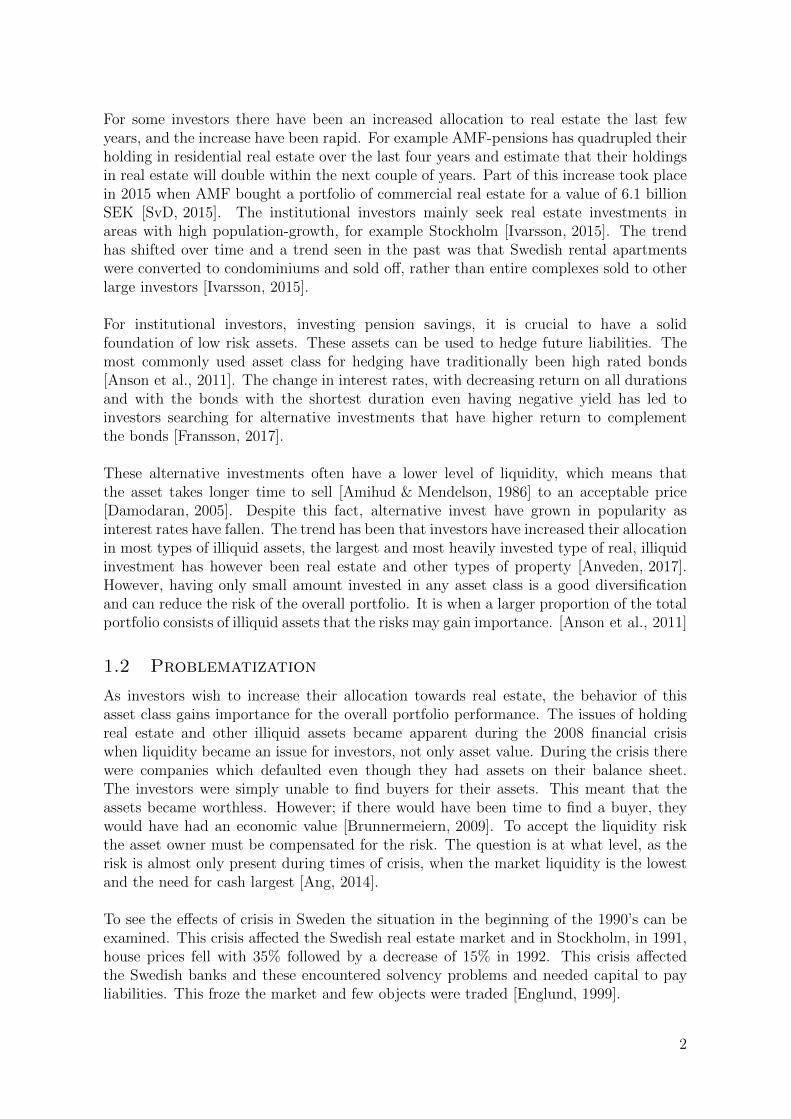
For some investors there have been an increased allocation to real estate the last few
years, and the increase have been rapid. For example AMF-pensions has quadrupled their
holding in residential real estate over the last four years and estimate that their holdings
in real estate will double within the next couple of years. Part of this increase took place
in 2015 when AMF bought a portfolio of commercial real estate for a value of 6.1 billion
SEK [SvD, 2015]. The institutional investors mainly seek real estate investments in
areas with high population-growth, for example Stockholm [Ivarsson, 2015]. The trend
has shifted over time and a trend seen in the past was that Swedish rental apartments
were converted to condominiums and sold o↵, rather than entire complexes sold to other
large investors [Ivarsson, 2015].
For institutional investors, investing pension savings, it is crucial to have a solid
foundation of low risk assets. These assets can be used to hedge future liabilities. The
most commonly used asset class for hedging have traditionally been high rated bonds
[Anson et al., 2011]. The change in interest rates, with decreasing return on all durations
and with the bonds with the shortest duration even having negative yield has led to
investors searching for alternative investments that have higher return to complement
the bonds [Fransson, 2017].
These alternative investments often have a lower level of liquidity, which means that
the asset takes longer time to sell [Amihud & Mendelson, 1986] to an acceptable price
[Damodaran, 2005]. Despite this fact, alternative invest have grown in popularity as
interest rates have fallen. The trend has been that investors have increased their allocation
in most types of illiquid assets, the largest and most heavily invested type of real, illiquid
investment has however been real estate and other types of property [Anveden, 2017].
However, having only small amount invested in any asset class is a good diversification
and can reduce the risk of the overall portfolio. It is when a larger proportion of the total
portfolio consists of illiquid assets that the risks may gain importance. [Anson et al., 2011]
1.2 Problematization
As investors wish to increase their allocation towards real estate, the behavior of this
asset class gains importance for the overall portfolio performance. The issues of holding
real estate and other illiquid assets became apparent during the 2008 financial crisis
when liquidity became an issue for investors, not only asset value. During the crisis there
were companies which defaulted even though they had assets on their balance sheet.
The investors were simply unable to find buyers for their assets. This meant that the
assets became worthless. However; if there would have been time to find a buyer, they
would have had an economic value [Brunnermeiern, 2009]. To accept the liquidity risk
the asset owner must be compensated for the risk. The question is at what level, as the
risk is almost only present during times of crisis, when the market liquidity is the lowest
and the need for cash largest [Ang, 2014].
To see the e↵ects of crisis in Sweden the situation in the beginning of the 1990’s can be
examined. This crisis a↵ected the Swedish real estate market and in Stockholm, in 1991,
house prices fell with 35% followed by a decrease of 15% in 1992. This crisis a↵ected
the Swedish banks and these encountered solvency problems and needed capital to pay
liabilities. This froze the market and few objects were traded [Englund, 1999].
2

The risk of not being able to trade assets or it taking long time to do so, can cause
problems. Periods of few or no trades are not seen in indexes and these therefore
creates di�culties in determining the true volatility of the asset. In the investment
spectrum of real estate and other illiquid assets, an asset only has a value at the time
of the transaction. At other times, when there are neither sellers nor buyers in the
market the asset has no tangible value. This leads to the e↵ect that most indexes
and other sources of continuous valuations are forced to interpolate between values of
similar assets and times which in turn may lead to the volatility being artificially low
[Edelstein & Quan, 2006].
If institutional investors are to increase their allocation towards illiquid assets, it is im-
portant to understand what return that can be expect for a certain level of risk and
liquidity. Another issue when shifting towards more illiquid investments is that this may
change the risk characteristics of portfolios; from a purely volatility based portfolio risk to
a portfolio with several risk factors. As most institutional investors are subject to control
of the Swedish FSA, know as Finansinspektionen (FI). They need to be able to report
predicted risk and return for their portfolio, and without a strong motivation behind their
assumptions they will be subject to harder capital requirements [Svensk forsakring, 2011].
To know if an investment is worth its risk it is important to know the expected risk and
return trade-o↵ for each asset. This will assist in making better informed decisions, which
hopefully in turn leads to higher pension benefits for the members.
1.3 Purpose and research questions
The purpose of this study is to investigate the e↵ects of giving up liquidity in the
portfolios of institutional investors. These e↵ects primarily include risk measurements
for liquidity and how liquidity risk can be quantified. The investigation of the e↵ects
is conducted in order to determine a level of required compensation, investors should
demand to make an investment in an illiquid asset, in particularly real estate assets.
The purpose of the study will be met through answering the following research questions
with the first two being more specific and the third research question more overarching
of the field.
The questions that this study will answer are:
• What risk factors does real estate contribute to a portfolio?
• How much of the total real estate risk can be explained by illiquidity and how can
illiquidity risk be calculated?
• What aspects in the overall portfolio a↵ects institutional investors ability to invest
in illiquid assets?
1.4 Limitations
We have selected to focus the work on the illiquid assets and in particularly real estate
assets. This limitation is set in place as real estate is an asset class which has grown in
3
popularity amongst pension investors [Cameras, 2017]. This asset class has risks which
are quite di↵erent from those risks associated with stocks and bonds [Brodin, 2017].
With this limitation, the focus of this study will be to investigate the e↵ects of shifting
from liquid assets to illiquid assets in the form of real estate.
When analyzing potential investments, which investment asset is most suitable will to
a high extent be dependent on the individual investor and their investment strategy
[Berk & DeMarzo, 2014]. All investors have di↵erent conditions with di↵erent investment
horizons and varying portfolio sizes. This study will be limited to institutional investors,
mainly pension funds. The main reason for this limitation is because of their sizes and
amounts of capital which makes them able to make larger investments. Pension funds
have a long time horizon, large amounts of assets under management and requirements
to meet in terms of return and overall portfolio risk [Anveden, 2017]. These aspects make
their investment strategies stand out from other investors; for example retail investors or
short time horizon investors.
This study is conducted in Sweden and has also been limited to this geographical area,
this limitation is used as there are di↵erences between markets. General assumptions will
be found globally but the research will be based on the transformation on the Swedish
market and what implications it has on the Swedish market. Regulations and market
conditions also di↵er between countries and are important factors for the investors. We
are aware that the regulations and capital requirements which a↵ect the target group
for this study change frequently, and the relevance would be reduced if the regulations
change, we have limited the study to current requirements but we have discussed the
potential e↵ect of regulatory changes that are currently being investigated.
1.5 The study’s contribution
One of the first influential studies on risk premiums was presented by Mehra and
Prescott when they introduced the puzzle of risk premiums in 1985. Since Mehra and
Prescott’s publication many studies have focused on estimating the risk premium for
stocks [Pastor & Stambaugh, 2003], [Amihud & Mendelson, 1986]. However, the focus
on risk premium for alternative investments has been limited in previously conducted
studies. An alternative investment which has received some attention is real estate
[Edelstein & Magin, 2012]. A few studies have been conducted on the risk premium in
real estate, but to the best of our knowledge no previous studies have been conducted
on the risk premium from real estate investments on the Swedish market and to what
extent the liquidity influence the overall risk.
The area of liquidity premium in real estate and other alternative assets is fairly unex-
plored and the limited previous studies conducted have come to varying conclusions. This
is partly because the definition of liquidity di↵er between researchers but also depending
on methods and data used for the studies. Studies from the Netherlands and United
Kingdom has discussed and developed the risk that arise from the unknown transaction
period and asset liquidity [Bond & Huang, 2004], [Bond et al., 2007]. To the best of our
knowledge, the area of liquidity risk and return from real estate on the Swedish market
have not been researched prior to the start of this work. This study aims to build on the
framework of Bond and Huang [2008] and apply their model to the Swedish market with
4

an addition of a qualitative analysis of concerns with investing in the asset class. This
study can then contribute with a more complete overview of the risks associated with real
estate.
5

2 Method
In this section of the report the methodology is described together with the research design.This describes the process of the study and also brings up considerations with for exampleresearch ethical guidelines and how these have been applied to the study together withreliability, validity and generalizability.
2.1 Research design
The method designed is to answer the research questions of including real estate in
a portfolio and quantifying the risks this brings to an asset portfolio, including the
liquidity risk factor. The initial step was to conduct a literature review which was
designed to give an understanding of the potential risks that are present within real
estate investments and how these are quantified. The method also included interviews
with institutional investors, real estate companies, bank representatives and specialists
to gain a better understanding on the investors opinions and their situations. In the
next stage the liquidity risk was calculated using quantitative methods, this stage
was conducted through an analysis of historical data. Historical data is used to valu-
ate the liquidity risk for alternative investments and comparing the risk with their return.
The work has been based on a deductive process and findings from the quantitative study
are compared to findings in literature and interviews. Through the quantitative approach,
general results can be found [Collis & Hussey, 2013] and this design serves the purpose
of the study well. The qualitative part of the study is to answer the research question
of the implications allied by alternative investments for institutional investors. However,
using a deductive design, being critical becomes less natural [Collis & Hussey, 2013] and
we have aimed to maintain critical throughout the research process as well as being open
to reflections and opinions.
2.2 Research process
The work process of this study has been divided in to seven steps. The process is presented
in chronological order, however, some of the steps were overlapping or conducted in
parallel.
• Pre-study - In the pre-study the literature review was started. Two interviews
were conducted to get a broader understanding of the subject and what the industry
require more information about. From the pre-study the preliminary background,
problematization and research questions was formulated.
• Literature review - Based on the research questions the literature review was
continued and more focused. Concepts and theory was identified which could be
further modeled and analyzed. The literature review was continued throughout the
research process but with a majority conducted in the initial stages.
• Interviews - From the theory, questions were formulated which are of interest for
the interview section of the study. Semi-structured interviews were then conducted
with institutional investors, real estate companies, bank representatives and spe-
cialists.
6
• Data collection - Data was collected from the database Bloomberg, Nasdaq OMX
Valueguard-KTH Housing Index (HOX) Sverige and MSCI:s IPD database. The
data included historical stock, bond and real estate prices. All data used were
collected in index form to give a generalized market view rather than object specific
view.
• Quantitative analysis - With the collected data and based on the theory a quan-
titative analysis was conducted through using models to quantify the impact of risk
factors.
• Analysis - The material collected from the empirical study together with the quan-
titative results were then compared and analyzed with theoretical findings.
• Conclusions - The results and analysis were then concluded to answer to the
research questions.
2.3 Literature review
Literature on the subject was collected throughout the process but with a focus in the
early stages of the research process. The literature review started of with a broad scope
and was narrowed down as the research process evolved. The literature was collected
through databases such as; KTH Primo, Google Scholar, Google Books and the Diva
portal. The literature included information from journals, articles and books. All
literature have been critically selected and when possible peer-reviewed processed papers
have been used. As the topic is specific and the field of liquidity in real estate has not
been broadly researched in Sweden, sources from other markets have been used. Most of
the studies conducted within the relevant areas are based on data from the American
market, but we have also used literature on studies conducted in the Netherlands and
United Kingdom. There are some di↵erences between the structures of the separate
markets, including the size of the market and regulations impacting the market. We are
aware of these di↵erences and take this into consideration when using foreign studies,
literature and findings. The following search words are words that have been included in
the search process:
Illiquidity, real estate, institutional investors, IPD-data, HOX-index, valuation, return,risk premium, illiquidity premium, risk appetite, risk management, asset management,asset liability management, asset pricing, performance, commission, transaction cost,transaction process, holding period, investment horizon, forced sales, investment struc-tures, classification of real estate.
2.4 Interviews
As part of the pre-study two interviews were conducted to gain a broader background
knowledge. The first interview was an unstructured interview with the department of
institutional advisory at SEB. The second interview was with a former PhD student in
Real estate economics and now director and financial adviser in property investments,
this interview was semi-structured in style. The interviews belonging to the pre-study
were not recorded, however, notes were taken during both interviews.
7

To get a deeper understanding of the real estate market and the institutional investors’
views on real estate and their strategies when investing in the asset class, further inter-
views with real estate firms and institutional investors were performed. These interviews
provided information with regards to the aim to increasing allocation to real estate and
other illiquid asset classes. During these interviews information regarding expected hold-
ing period of their investments and the expected transaction times for the holdings in the
illiquid asset classes, in particular real estate, were also collected. The expected holding
and transaction period are required input data for modeling liquidity risk and information
which is not available through data bases, this material was therefore collected through
interviews.
2.4.1 Interview selection
The interview participants were selected to represent a diverse group with varying
views, strategies and concerns regarding real estate investments. Through including real
estate firms the process of direct investments could be understood and how a decision is
taken and which factors are important when investigating in individual objects. From
interviews with institutional investors and institutional sales the portfolio perspective
of holding alternative investments could be understood. In the expert interviews other
considerations and approaches were brought up.
The selection of some interviews was based on recommendations from our contact person
at SEB. The selection also included AP funds as these have a large diversified portfolio
and a long tradition of a fairly large allocation towards real estate, AP2 was excluded
on account of their geographical location. The interviews have been limited to actors
with their head o�ce in Stockholm due to travel considerations. This may be a factor
that impact our findings as the market which we have investigated are regional and may
di↵er between areas in Sweden.
Real estate companies were also include in the interviews and the selection of real estate
companies were based on company size. We also included geographical considerations
when selecting real estate firms and also here limited the selection to Stockholm. Three
real estate companies were finally selected to participate in the interview section. In
addition to the previously mentioned interviews an interview was conducted with a
smaller pension fund. This interview could contribute with the perspective of how the
size impacts the view on real estate investment.
All conducted interviews are summarized in the following table:
8

Date Name Position Company Format20/1 M. Anveden Institutional Advisory SEB Unstructured26/1 J. Lekander PhD in Real Estate Economics KTH Semi-structured17/2 J. Skogestig Head of Real Estate Investments Vasakronan Semi-structured20/2 H. Brodin Institutional Sales SEB Semi-structured21/2 B. Hellstrom Alternative Investments AP3 Semi-structured22/2 R. Gavel Real Estate Portfolio Manager SEB Semi-structured23/2 F. Salen Broman Portfolio Analyst SEB Semi-structured3/3 M. Cameras Transaction & Analysis AMF Semi-structured6/3 A. Bergstrom Head of Finance Fabege Semi-structured6/3 K. Hansen Vikstrom Head of Business Development Fabege Semi-structured10/3 M. Angberg Chief Investment O�cer AP1 Semi-structured15/3 T. Fransson Alternative Investments AP4 Semi-structured15/3 O. Nystrom Asset Manager; Real Estate AP4 Semi-structured23/3 A.Evander Chief Investment O�cer FPK Semi-structured30/3 C. Gustafsson Executive Director MSCI Semi-structured3/5 G. Marcato As. Pr. Real Estate Finance HBS Semi-structured
Table 1: Interview schedule
The reliability of a study is increased with larger number of interviews, we did however
reach an empirical saturation in our findings. As well as the empirical saturation we had to
limit the total number of interviews held because of time considerations and having more
interviews would have added diminishing marginal utility for each additional interview.
We fulfilled the number of conducted interviews stipulated by Backer and Edwards [2012]
which suggests between 12 and 60 interviews for a case study based graduate thesis. We
have positioned the total number of interviews within this range, but are also aware that
we are in the lower range of the spectrum. For this study interviews are however only
one section of the study in combination with a quantitative approach.
2.4.2 Structure
All non pre-study interviews with the exception of three interviews were recorded, and
notes were taken during all interviews. We did not, unless specific quotations were
taken, transcribe the full length of the interview. After the interview the notes taken
were, if needed, supplemented with transcriptions from the recordings. When asked
for, the interview questions were sent in advanced to the interviewed persons, but for
most interviews the questions were not requested. After the interviews the material was
categorized and compiled, from the characterization conclusions and results could be
found.
The semi-structured format, which was used for all except one interview, suited the study
well as this format gave a basis of preparation of what the discussion was going to be
about. With the possibility of asking additional questions clarifications could be made
and the answers followed up to gain more information where the interviewee had more to
add [Collis & Hussey, 2013]. One concern with this format is that the follow up questions
posed during interviews di↵er between the participants and thereby reduce comparability
between interviews. However the semi-structured format give the possibility to go into
depth in the area of interest for the person and get additional insights.
9
2.4.3 Ethical considerations
During the interviews the research ethics principles by Vetenskapsradet [2002] has been
applied and followed. The four main ethical considerations will be developed below.
• Information - All participants in the interview section were informed of the purpose
of the study. When people were contacted and asked to participate in the interview
section of the study the work was described, selection motivated and the type of
questions going to be asked clarified.
• Approval - All interview participants approved to participation in written form
through e-mails after the question of participation were sent with a brief description
of the purpose of the study and the topic which was to be covered during the
interview. Participants were also asked for their approval regarding the recording
of the interview.
• Confidentiality - All participants were given the option to participate anony-
mously. In the study none of the participants requested to participate anonymously.
• Use of findings - All information collected for the study will only be used for
the purpose of this study. All participants were made aware that this study will
be public once finished. All recordings will be deleted after the completion of the
study.
2.4.4 Classification of empirical material
After the interviews the gathered material was collected and classified according to cate-
gory. Some questions asked during the interviews were used for the quantitative modeling.
The remaining information was used to understand the investors behaviors and other as-
pects of real estate investments. The material was classified into the categories: the
balance between risk and return in investments, illiquidty, transactions and the asset
from a portfolio perspective. The findings can be found in section 4.
2.5 Data collection
The qualitative section of the study is based on historical data. The data included in this
study are: historical stock, bond and real estate prices. Historical stock and bond prices
was obtained from the database Bloomberg. Finding historical data on physical real estate
is more challenging as there are only price information available when a transaction has
been conducted. Another problem with real estate data is that objects included in for
example indexes are not identical, unlike for example stocks. To combat this issue, data
on real estate indexes as MSCI’s IPD-index and Nasdaq OMX Valueguard-KTH Housing
Index (HOX) Sverige has been used. In addition, data on expected transaction period
and expected holding period was used, this data could be obtained through interviews
and deducted from data.
2.5.1 Housing index - HOX
The Swedish Nasdaq OMX Valueguard-KTH Housing Index (HOX Index) is based on a
hedonistic price model with monthly price updates. Data in the HOX indexes includes
privately owned flats. The data for the index is collected through Maklarstatistik AB, and
10

multiple regression is then used to adjust the transaction price for the descriptive factors
of the particular object sold. These factors includes indicators such as; size, number of
rooms and location and is used to calculate the price development for what is defined
as a ’normal property’. This method require less data then comparing transactions of
the same object, in which repeated transactions of the same object is used. An issue
with a hedonistic index is that it is subject to the appropriate definition of the model.
The weighing of the HOX index is adjusted every six month to appropriately reflect the
distribution of completed transactions. [Valueguard, 2011]
2.5.2 Property index - IPD
For data of di↵erent segments within real estate investments the MSCI Swedish annual
property digest was used. These data include historical index changes between the years
1983 and 2016. In this data real estate is categorized as retail, o�ces, industrial and
residential properties. The data is based on valuations and not transactions as other
indexes. It included in total 3937 properties in year 2016 [MSCI, 2016]. From the IPD
data bank only data on the Swedish market have been used, IPD data is updated annually.
2.5.3 Considerations with data
The transaction based HOX index gives an indication of price changes and the IPD
index on how the valuations are changing for the whole market and segments but not
for particular objects, and these indexes are not pure transaction data from re-sold
properties. The quantitative findings would have had a higher reliability for single
objects if the data used was only from that object. However, the general market trend
is more interesting for the study then specific cases and therefore the data used is
representative and serves the purpose of the study well.
Through collecting data from databases the study will be based on secondary data
[Collis & Hussey, 2013]. Part of the data is historical stock and bond prices. This is
public data which can be assumed to be accurate. Through using IPD index and HOX
index data their way of collecting data will have to be trusted and it is important to
understand what type of real estate that is included in the indexes and from what market
data is taken to make a comparable study.
A limitation in the real estate data used for the study is the infrequent reporting of
data. IPD data is only available on an annual basis and HOX on a monthly basis. This
limitation is however compensated for by the long time series available, giving enough
data to do reliable statistical investigations. The long time series also includes data from
several market cycles. Using historical data to predict future outcomes is another limiting
factor in all forward looking studies. We will use historical data as a proxy for future
outcomes and the applicability of this will be limited to the assumption that historical
information is a good proxy for future events.
2.5.4 Smoothed data
Real estate data have the bias of insu�cient transaction data during recessions. Data
on prices in real estate only become public when a transaction is successful. This
makes data biased as failed trades and desolated properties are not included in the
11

index [Edelstein & Quan, 2006]. In addition valuation based indexes, as the IPD-
index, have the problem that the fluctuations in price can not always be visible in
the data. This can be caused by the fact that valuations di↵er from actual market
prices and have a time lag. The time lag arise as valuations are based on previous
valuations and not carried out so frequently. These factors make real estate valua-
tions smoothed. To be get comparable real estate investments the de-smoothing was
conducted to compensate for the issues arising from real estate valuations [Geltner, 1992].
In order to adjust for indexes being based on valuations rather than transactions, the
approach of de-smoothing of real estate indexes is used. The theory behind this approach
is described in section 3.6.5. The other data set used, Nasdaq OMX Valueguard-KTH
Housing Index (HOX) Sverige is transaction based residential real estate data, as the
HOX-index is transaction based, no de-smoothing is used on this data.
2.6 Quantitative analysis
The data collected was then used for calculations in accordance with a model developed
by Bond and Hwang [2004]. Their model is designed to generate the ex-ante variance.
The ex-ante variance is the variance of both the holding- and the transaction period.
Based on the ex-ante variance model, a scaling factor for the variance can be calculated
from the index-data.
The adjusted variance can then be used for calculating an adjusted Sharpe ratio for real
estate, which then in turn can be compared to the Sharpe ratio for equities. Under the
assumption that all risks are rewarded, this is used to calculate how much of the real
estate return that should be allocated to the transaction period risk. This will however,
be an approximation as there are other risk factors that needs to be accounted for other
than liquidity risk and market risk.
In addition to these steps an investigation of the e↵ect of a potential forced sale on
the expected return for the asset as to investigate the risks associated with having less
liquidity and thereby having longer transaction periods. These calculations were carried
out on hypothetical cases formed by findings from the literature review and interviews. A
situation of forced sales can also be used to show up some of the implications for illiquidity
from which a liquidation bias premium can be calculated.
2.7 Source criticism
Throughout the work stringent source criticism have been applied. The literature used
has either been published in a journal or as a independent book by a known publisher.
To the highest degree possible more than one source have been used in order to confirm
the findings. Interviews or findings from this study have, in the cases where possible been
allowed as source confirmation. We have throughout the work aimed for triangulation of
all findings. Triangulation entail finding at least three independent sources of information
leading to the same conclusion [Collis & Hussey, 2013]. For most sections of this report
triangulation has not been possible as we only have literature and interviews supporting
our findings.
12

2.8 Validity and reliability
Validity is that the right thing is studied and part of this is that a suitable method is
chosen for the purpose of the study. Reliability is that the thing is studied the right
way, this can be how results are measured or interpreted [Blomkvist & Hallin, 2015].
Reliability is connected to the objectiveness of the researcher and to the extent another
researcher would come to the same conclusions [Collis & Hussey, 2013].
In the quantitative part of the study the reliability is high since both the method and
data used are presented and the study could therefore be replicated with the help of
publicly available data. Illiquidity is a term that can be interpreted in di↵erent ways
and researches do not have one definitive definition of what the term actually entail or
how it should be used. The di↵erent definitions of liquidity and what it actually is could
decrease the validity since going by Blomkvist and Hallins [2015] definition of studying
the right thing depends on the individual definition. To work with this it is important
to be clear when defining what definition we work with.
In the quantitative part of the study validity was created through having several, care-
fully formulated questions. The reliability was enhanced as during most interviews there
were two persons interpreting the answers from the interview and also having several
interviews. However, reliability decreases as a result of the semi-structured format of the
interviews and that di↵erent follow up questions were asked in di↵erent interviews. This
is not unexpected since results from research in social science rarely can be replicated
[Blomkvist & Hallin, 2015].
2.9 Generalization
The ability to generalize the findings from this study will be limited due to the limitations
described in section 1.4. The models used is however generalizable and the method used
are suitable for use in wider markets. As the interview section is designed to account
for the specific market conditions in the Swedish market and the regulatory conditions
of this market, the interview findings should not be considered generalizable to a wider
market, but can be used for comparable purposes between markets. With regards to
other investor types the findings are limited to investors with a long time horizon and
large amounts of capital under management, a generalization past this group would not
be possible due to the inherent aspects of real estate investments.
13

3 Theoretical background
In this section of the report previous literature and studies conducted within the field arepresented. This includes mathematical and theoretical frameworks which are to support theresearch questions. The frameworks include Sharpe ratio, characteristics, categorizationand factors of liquidity, ex-ante variance, liquidation bias and risk frameworks.
3.1 Traditional asset pricing
Investments in di↵erent assets face di↵erent risk factors. The return from an invest-
ment is expected to increases as the risk associated with the asset increase and the
more risk an investor is willing to accept the larger is the potential portfolio return
[Berk & DeMarzo, 2014]. Several models have been developed to calculate the expected
return on traded investments and the models usually refers to traded stocks as the risky
investment [Cornelius et al., 2013]. To compare the risk with the return from a particular
asset the Sharpe ratio is a measure commonly used. The Sharpe ratio is calculated as
follows [Sharpe, 1964];
Sharpe ratio =Expected return�Riskfree rate
Standard deviationWhen assets are priced the pricing is usually based on the expected return of the asset
based on its expected future cash flow. For pricing the Capital Asset Pricing Model
(CAPM) is a model frequently used. From this model an assets price can be calculated
form the underlying parameters of; risk-free rate, the expected market return and how
the asset is moving in comparison to the market (�) [Brennan, 1998]. Fama and French
[2015] extended CAPM and originally developed the three factor model from which stock
returns could be explained by company size, price to book value and market risk. The
model has continuously been developed, the model currently include up to five factors
[Fama & French, 2015].
One extension which has been added to the three factor model developed by Fama
and French has been to include liquidity. This extension is to account for the liquidity
premium in stocks. The descriptive factors which is used to account for liquidity include
for example trading volume and bid-ask spread amongst a multitude of factors. Bid-ask
spread and trading volume are parameters that are measurable on the stock trading
markets but these parameters on alternative investments are not readily available or
measurable from available data [Pastor & Stambaugh, 2003].
Considering the underlying performance and expected return from stocks the general
ideas are the same also for alternative investments with a lower level of liquidity. The
price is set from future payouts, how the asset class is performing in comparison to the
market and what risk the investment imply [Brennan, 1998]. Just like with stocks leverage
can be used to increase the expected return through increasing the exposure towards the
underlying risky asset [Lang et. al., 1996].
3.2 Allocation decision
Assets perform di↵erently depending on which risk factors it is exposed to and through
a combination with assets exposed to other risk factors the overall portfolio risk can be
14

reduced for a expected return than individual assets give at the same risk and an optimal
portfolio is then created, this is known as di↵erentiation. For e↵ective di↵erentiation the
correlation between assets is of importance. The overall portfolio risk reduction increase
as correlation between assets in the portfolio decrease, optimally a correlation of minus
one would remove the total risk.
Traditional portfolio optimization is carried out through the mean-variance optimiza-
tion framework where an e�cient frontier is found based on the correlation between
assets and each assets individual risk and return profile. The investor can then from
the e�cient frontier select the portfolio which best fit their portfolio requirements
[Berk & DeMarzo, 2014].
3.2.1 Institutional investors portfolio management
Portfolio management di↵er between individual investors and institutional investors
also in that institutional investors usually have a liability side in their portfolio. For
pension funds with future payments other approaches of assessing what the optimal
portfolio would be is through the Asset Liability Model (ALM) or Asset Only Model
(AOM). In the ALM framework the aim is to match the assets with the liabilities, both
in terms of size and duration. In the AOM framework only the assets are considered
[Hoesli et al., 2003]. Hoseli et al. [2003] finds the optimal allocation to real estate ranges
between 15-20% in a AOM framework and the optimal allocation in an ALM framework
is around 10%. The range is depending on the investors ability to accept di↵erent risk
levels in the portfolio. The same study also found that the actual allocation to real estate
among pension funds in Sweden is about 8% which is lower than the range suggested by
either optimization framework [Hoesli et al., 2003].
A presumption for e↵ective portfolio management is that the portfolio can constantly be
re-balanced and that way always strive towards an optimal allocation. Investing in less
liquid assets implies a risk for the investor as the portfolio will lose some of its ability
for continuous re-balancing. To compensate for this the investors demands a premium to
take on the re-balancing risk. [Cornelius et al., 2013]
3.3 Illiquidity
The definition of the term liquidity vary between studies. An illiquid asset is in simple
terms an asset which is harder to sell than a liquid asset. The harder it is to sell an asset
at market price the more illiquid the asset [Amihud & Mendelson, 1986]. Anson et al.
[2011] define an illiquid asset as an asset which takes time to convert into cash. Liquidity
can also be described in terms of the ability to trade large volumes of the asset without
impacting the price and to being able to trade at a low cost [Pastor & Stambaugh, 2003].
Damodaran [2005] on the other hand claim that the term illiquidity is occasionally mis-
leading since all assets can be traded at all times; it is just a question of what price the
seller is willing to accept. Meaning that there are no truly illiquid assets, it is just a scale
depending on how much reduction in price the seller would have to accept to trade at
a give time. The issue with falling prices at the time of transaction is often referred to
as price impact. Damodaran defines illiquidity through the cost that would appear if a
reversion of a decision occurs and a trader who bought an asset would immediately sell
15

the asset. Damodaran [2005] claim that the price impact can be used to measure liquidity
of a particular asset. A frequently traded, publicly owned asset has a low risk of implying
high transaction costs, and thereby have low price impact. What cost there will be for
completing an transaction is dependent on the number of potential buyers but can also
di↵er between financial securities and real assets [Damodaran, 2005].
3.4 Real estate as illiquid investment
Investing in real estate can have characteristics and bring risks other than those from
traditional assets such as stocks or bonds. Real estate is considered an illiquid investment
according to some of the definitions above [Girling, 2013] [Ang, 2014]. The part of the
risk that can be measured in assets is related to the volatility, but for some investments
there is also a part that is related to uncertainty. It is the uncertainty or immeasurable
risk that generate liquidity risk [Cornelius et al., 2013]. When it comes to stocks,
liquidity is a↵ected by three factors. These factors are; the price impact, that is the
transaction cost the investor will have buying or selling and asset, the bid-ask spread
and the opportunity cost for waiting of completing the transaction [Damodaran, 2005].
Ametefe et al. [2015] identify five characteristics that can be used to describe liquidity
and which could also be used for alternative investments, including real estate:
• Tightness - The cost of trading
• Depth - The ability to trade without impacting the price
• Resilience - How increased trading quantities is a↵ecting the speed at which the
marginal price changes
• Breadth - The total volume traded
• Immediacy - The cost arising when having to sell an asset quickly.
Figure 2: Graphical representation of liquidity characteristics
Source: Ametefe et al. [2015]
16

3.4.1 Methods of investing in real estate
Investing in real estate can be done in four main ways, each with di↵erent levels of
liquidity, these are; direct through private equity, public equity through for example Real
Estate Investment Trusts (REITs), public dept as Mortgage Backed Securities or private
debt as direct lending [Lekander, 2016].
In addition fund structures can be used to gain exposure to real estate or for investing
in the asset class. These fund structures can either be structured as open or close ended
funds. A close ended fund has a date of maturity and money can not be withdrawn
until this date [Russell, 2007]. An open ended fund has got the option to issue or redeem
shares at any time. This means that investors buy into the fund from the issuer rather
then in a market place with the price of each share issued directly represent the market
capitalization of the fund [Edelen, 1999].
3.4.2 Reasons to invest in real estate
The decision to invest in real estate can come from di↵erent portfolio requirements for
di↵erent investors and these investors therefore select di↵erent ways of investing in the
asset class. Investments in real estate can for example be included in a portfolio to give
returns higher than interest rates, global investment opportunities or as a way of receiving
stable cash flows [Anson et al., 2011]. The value created in the real estate industry comes
from the demand for a place to live or operate and the asset holders get a yield from
rents paid and maybe also return from increased asset value [Baker & Chinloy, 2014].
Investing in real estate can also provide good portfolio di↵erentiation as it is connected
to other kinds of the systematic risk factors than stocks and bonds, for example liquidity
related risk factors [Anson et al., 2011]
Another reason to invest in real estate is according to Anson et al. [2011] the inflation
hedge real estate assets can provide as rent levels are often adjusted for inflation, i.e. the
rent increase with inflation during the duration of the contract. The inflation hedge that
real estate o↵er is a debated subject and Ang [2014] concludes that real estate a poor hedge
against inflation. During bad times in the market the liquidity in real estate objects will
go down, which will have a negative impact on the portfolio flexibility. Liquidity levels for
real estate assets are hard to draw general conclusions about since the liquidity depends
on location and characteristics related to individual objects.
3.4.3 Categorization of real estate
Direct real estate investments can be described in several ways. Objects di↵er, which
makes them hard to compare and a↵ects the level of risk in each object [Lekander, 2016].
The CAIA Association [2016] has created a classification of real estate objects by eight
characteristics, these are;
1. Property type - what the building is used for
2. Life-cycle phase - if the object is newly built or an existing building
3. Occupancy - if there are tenants or if the building is vacant
4. Roll over concentration - frequency of trades in the asset
17
5. Near term rollover - probability for trade in near future
6. Leverage - if loans are taken to finance the investment
7. Market recognition - the extent to which the asset is known to institutions
8. Investment structure - the extent of control and governance
Based on these eight real estate characteristics objects can be divided into three sub
groups; Core-, Value-added- and Opportunistic real estate. A real estate portfolio with
objects from the Core sub group will have low leverage and an open-ended structure. This
type of portfolio has stable returns and comparatively low risk. A Value-added portfolio
can consist of a mix of value-added and other investments and more leverage, up to about
fifty percent. In a Value-added portfolio incomes are less stable and the risk level higher
than in a Core portfolio, because of the higher risk the expected return is also higher.
The third type of portfolio is the Opportunistic, which has higher risk and where a higher
return is demanded. The risk can come from several sources, some are; high leverage,
leasing risk and development risk [CAIA Association, 2016].
3.5 Risk compensation for liquidity
When trading in illiquid assets the investors face risks which need to be compensated
for. Most illiquid assets are a↵ected by a illiquidity discount. The size of the illiquidity
discount is e↵ected by both the transaction cost and the expected holding period for the
asset. The longer an investment is expected to be held, the lower the illiquidity discount
and the higher the transaction cost, the larger the illiquidity discount. This e↵ect is
quite self-explanatory as if an asset is traded with a 5% transaction cost and expect
to be held for one year, the asset would have to at least increase 5% in value for the
investment to break-even [Damodaran, 2005].
The exogenous transaction costs i.e. the direct transaction costs such as brokerage fees
and transaction taxes a↵ect the liquidity of the asset. The direct costs are however not
the only costs that arise when trading in illiquid assets, there are also costs that arise
from the risk that illiquidity brings [Easley et al., 2000]. These liquidity risks include
demand pressure and inventory risk. Inventory risk arises from the risk of not getting the
asset sold when wanted. Demand pressure is the risk for the investor of not finding the
right buyer at the time when the investor wishes to sell [Easley et al., 2000]. Liquidity
problems usually arise in periods of market turmoil, for example that could be when
bubbles burst or changes in the risk concentrations [Carrel, 2010].
3.5.1 Liquidity premium
Previous studies on the area of liquidity premium in alternative investments or real es-
tate are limited as discussed in the introduction and no studies have been found on the
Swedish market. The few studies that have been carried out comes to di↵erent conclu-
sions depending on how liquidity is defined and how this is calculated. Ang [2014] finds
the yearly liquidity premium for inflation protected securities to be around 0.5% with a
peak of 2.5% during the 2008 financial crisis. Hordijk and Teuben [2008] on the other
hand finds the annual liquidity premium in the Netherlands to range between 0.09% -
0.31%. Marcato [2015] concludes that the premium is around 3% in the United Kingdom,
but varying between 1.5% up to 10% depending on market conditions.
18

3.6 The illiquidity risk in real estate
The liquidity risk in real estate can arise from di↵erent liquidity factors. Hordijk and
Teuben [2008] have divided the liquidity risk associated with real estate investment into
five risk liquidity risk factors, these are:
• Opportunity risk
• Liquidity risk for incomes
• Accurate valuation risk
• Heterogeneity risk
• Transaction process risk
These factors will furthered be explained in the now following sections.
3.6.1 Opportunity risk
The opportunity risk is the risk of missing other investment opportunities because of
the decision to allocate money to a particular asset. With variables for the return from
an alternative investment during the holding period and the transaction period (Eh+t),
the return of real estate during the holding period (Rh) and the incomes during the
transaction period (Rt). [Hordijk & Teuben, 2008]
Opportunity cost = Eh+t � (Rh +Rt)
3.6.2 Liquidity risk of incomes
The liquidity risk of incomes is the risk that properties become vacant and therefor not
generating the expected cash flows. This could for example happen if tenants defaults or
in some other way not are able to pay their rents [Hordijk & Teuben, 2008]. This can be
considered as a counter party risk factor [Girling, 2013]. The liquidity risk of income is
a↵ected by the number of possible tenants and the attributes of the object. According to
the CAIA Association [2016] and their classification of attributes this risk is largest for
Opportunistic objects in comparison to Core investments which have a lower degree of
liquidity risk of incomes.
3.6.3 Heterogeneity risk
Another component in liquidity risk is the heterogeneity risk. That is the di�culty in
comparing objects, as each property is unique. Units of real estate di↵er and there are
more di↵erences compared to trading one stock which is always the same, given the same
class and company. Within the real estate investment spectrum it is not only the object
that di↵ers, there are di↵erent ways to invest in real estate as for example o�ce buildings
or residential buildings and to direct or indirectly in the asset. Hordijk and Teuben [2008]
argue that heterogeneity risk is not of big importance to the overall risk. Heterogeneity
risk can in some cases also be connected to the concept of information imbalance as you
do not know what you get when you but a property.
19

Information imbalance - A problem which is present in illiquid transactions is the
information imbalance between the buyer and the seller which is causing an information
gap. In the real estate case it is common that the seller knows more about the asset
than the buyer. This leads to a risk for the buyer, that the seller is selling based on some
private information [Easley et al., 2000]. In order to combat this issue, there is commonly
a due diligence period when doing large transactions. The due diligence process aim to
give the buyer increased knowledge of the property and reduce the risk that the seller
had private information which would drastically reduce the property’s value. The due
diligence period is costly and contributes to the high transaction cost as well as it increase
the transaction period [Roulac, 2000].
3.6.4 Accurate valuation risk
Studies have shown that there is often a discrepancy between the latest valuation and
the sales price [Geltner, 1992], [Englund et al., 1999], [Kaplan, 2012]. The pattern that
has been seen is that the last valued price usually is lower then the sales price, it should
be added that this pattern have been obtained in a period of a positive market trend
and it might be di↵erent to results in falling markets. The di↵erence between sales
price and appraisal can be divided into two factors; a lagging error and a random error.
The lagging error is dependent on the market development since the appraisal date.
The random error consist of the time lag, information lag and a random error term
[Hordijk & Teuben, 2008].
The valuation risk i.e. the risk that assets can not be sold at the appraised value can be
explained by two factors: market debt and nonlinearity of market functions [Carrel, 2010].
Market depth is the volume that can be traded without a↵ecting the market prices or
spreads. Nonlinearity of the market function is the lack of information during the transac-
tion period. The lack of transparency in the real estate market makes it hard to estimate
prices in the market and is dependent on the time horizon and purpose for the trade and
therefore a↵ect the valuation of assets and the value of the portfolio.
3.6.5 De-smoothing real estate returns
To compensate for the di↵erence between the appraised value and the price obtained at
transaction a method referred to as de-smoothing is commonly used. Smoothing is the
process when peaks and lows of values are not as high or low as they would have been
if transactions were used. One reason for the smoothing is that the valuations are slow
in responding to changes in the market and valuators are cautious when valuating a
property. The de-smoothing process can also be used to compare value based real estate
indexes and transfer these to comparable transaction prices [Geltner, 1992].
Kaplan [2012] finds evidence for the smoothing caused by appraisal and motivates this
by the historical performance of stocks, bonds and real estate between the years 1926
until 1992 on the American market. During this period stocks gave a return of on
average 10.5% and real estate 8.5% per year. At the same time real estate produced
a risk lower than that from bonds and without correlation to either stocks and bonds.
This would imply that real estate is a superior investment and the e�cient portfolio
should only consist of real estate. This have not been the case and Kaplan [2012]
motivates this by the smoothing taking place caused by the appraisal process. Evidence
20
of auto-correlation between data points of returns has also been found on the Swedish
market [Englund et al., 1999].
In order to combat issues with data auto-correlation the process of de-smoothing can be
applied to the data. The de-smoothing process aims to return the variance which is at
the risk of being eliminated through the valuation process. The formula for de-smoothing
can be written as [Geltner, 1992]:
Vt = ↵Pt + (1� ↵)Vt�1. (1)
In the de-smoothing process the value at time t is Vt, and can be calculated as a function
of the valuation one time unit before and a factor for comparable sales taking place at
the same time. To balance these two factors a de-smoothing factor (↵) is introduced
[Netzell, 2010]. The de-smoothing factor (↵) is time and situation dependent. Geltner
[1992] finds that ↵ usually range between 1/2 to 2/3. From equation (1) the de-smoothed
value Pt can be found:
Pt =Vt
↵� (1� ↵)Vt�1
↵. (2)
The main concern with using the de-smoothing process described above is that it is
dependent on the choice of (↵), which can not be determined from factors measurable
in the market. The larger the value of alpha the larger the variance in the de-smoothed
time series [Netzell, 2010].
3.6.6 Transaction period risk
Transaction period risk is the uncertainty of how long the marketing period will be from
the time of the decision to sell an asset. This uncertainty gives rise to other risk factors
than those that can be measured using for example standard deviation. Bond and Huang
[2004] formulated a method for calculating the volatility during the transaction period.
They claim that real estate indexes tend to overlook the excess risk that arise from
an unknown transaction period. The uncertainty leads to real estate as an asset class
having higher risk than that which can be seen through measuring the index volatility.
The transaction process risk measure, ex-ante variance, aim to give a measure by which
the volatility can be scaled to appropriately represent the risk during both the holding
period and the transaction period. This measure does not account for the other risk
factors that may a↵ect the total risk for illiquid assets.
The transaction period risk is dependent on two main factors; the expected holding period
and transaction period [Bond & Huang, 2004]. The average holding period for o�ces
and retail real estate is around 13 years and approximately 25 years for residential real
estate on European markets [Collett et al., 2003], [Hordijk & Teuben, 2008]. In stock
markets the implied holding period is usually calculated as the outstanding volume of
shares divided by the traded volume [Atkins & Dyl, 1997]. Collett et al. [2003] have
correspondingly formulated a formula to calculate the implied holding periods from IPD
data of real estate. This approach is limited as di↵erent assets have di↵erent holding
periods as some are traded frequently and other less frequently. This approach is also
limited as the institutions reporting to IPD can change during years. However, Collett
et al. [2003] come to the conclusion that this measurement can be used as a proxy for
21

implied holding period as only studying individual transactions would miss out on objects
not getting sold.
Holding Periodt =(Nr. of Propertiest +Nr. of Propertiest�1)/2
Salest(3)
Based on IPD-data Hordijk and Teuben [2008] come to the conclusion that the transaction
period in the Netherlands is usually between two and six months. They compare these
results to other European markets and find that they are similar in other countries in
Europe.
Figure 3: Transaction period
Source: Hordijk & Teuben, 2008
The decision to sell a real estate asset goes through the following steps in the transaction
process [Hordijk & Teuben, 2008]:
Figure 4: Transaction stages
Source: Hordijk & Teuben, 2008
3.6.7 Framework for calculating transaction risk
A framework for accessing the transaction period risk in illiquid investments has been
developed by Bond and Huang [2004]. Their framework is based on an assumption that
returns are normally distributed and that the transaction time follow a exponential dis-
tribution. From the distribution assumptions mean and variance for the return can be
calculated from available data. The transaction time can be estimated through informa-
tion from interviews. The following variables will then be introduced for calculation of
transaction risk;
22

Notation Explanation
h Holding period
t Transaction period
r Return
µ Average return
�2Variance of return
� Parameter for sales distribution
Table 2: Introduced variables
Ex-post risk and return is defined as the time the investment will be held before it is
sold, including the time for the transaction. The expected return and variance ex-post
is EP(rh+t) and V arP (rh+t). Ex-ante the risk of doing the transaction is not known and
this have to be compensated for in the terms EA(rh+t) and V arA(rh+t).
EP(rh+t) = E(rh+t|h+ t) = µ(h+ t) (4)
V arP (rh+t) = V ar(rh+t|h+ t) = (h+ t)�2(5)
In the ex-post formula the transaction period is known. This is not often the case in real
estate investments and this implies a transaction risk which is to be considered a liquidity
risk.
V arA(rh+t) = E⇣V ar(rh+t|h+ t)
⌘+ V ar
⇣E(rh+t|t)
⌘= E
⇣V ar(rh+t)
⌘+ V ar
⇣E(rh+t)
⌘
(6)
Using the expressions from (4) and (5) the equation can be rewritten as follows, where µe
is the expected sales period and �e the expected standard deviation for the sales period:
V arA(rh+t) = (t+ µe)�2+ µ2
e�2e =
1
(t+ h)
⇣(t+ µe) +
µ2
�2�2e
⌘V arP (rh+t) (7)
Under the assumption that the transaction time is exponentially distributed with param-
eter �. The expected time for transaction will be Poisson distributed with parameter �both the expected value and the standard deviation of the distribution is �.
f�(t) =e�t/�
�(8)
Insertion of this in the ex-ante formula gives;
EA(rh+t) = µ(h+ �) (9)
V arA(rh+t) =
⇣µ2
�2
�2
t+ �
⌘V arP (rh+t) (10)
The term which scales V arP (rh+t) to V arA(rh+t) is then the factor with which the variance
has to be multiplied with to include the transaction risk, i.e. the factor representing the
transaction process risk. This term will be refereed to as the ex-ante variance scaling
factor or the ex-ante scaling factor. The ex-post variance is the risk measurable in the
index over the holding period and transaction time.
23

3.7 Forced sales
Another component of liquidity presented in the model of Ametefe et al. [2015] is
immediacy. For an illiquid assets the risk of forced sale, or in some cases known as
fire sale, can result in considerable consequences. A forced sale is characterized by a
shorter transaction period than that required to obtain market price. The reasons for
forced sale vary, but it may be associated with an immediate demand for liquidity or
changing market conditions [Donner et al., 2016], [Campbell et al., 2011]. The cost of
liquidation in real estate is di↵erent to the financial market in which market prices can
be obtained instantly. This is a risk that is not reflected in the prices as most sellers
have been prepared for the transaction for a time and the price is then reflecting recent
prices [Lin & Vandell, 2007].
The cost of forced sale, or the reduction in price is highly dependent on market conditions
and the size of the reduction in transaction period. In a study on Swedish residential real
estate sold by the Swedish enforcement o�cer the reduction in transaction price is esti-
mated to range between 22% and 29% depending of the reason for the forced sale, which
also impact the average transaction time for the forced sale [Donner et al., 2016]. These
sales are mainly single family homes and not the larger lot sizes commonly associated
with institutional investors. This risk should however not be ignored for institutional in-
vestors either even thought few earlier studies have been conducted on the consequences
for institutions. Overall the liquidation risk premium for properties can be computed
through the model developed by Lin and Vandell [2007].
3.7.1 Liquidation bias premium
To compute the impact of liquidation Lin and Vandells [2007] measure, liquidation pre-
mium can be used. If transaction prices and market valuations are assumed to be
uniformly distributed the liquidation bias premium can be calculated as the di↵erence
between the transaction value and market value (µT � µM) with volatility bias as the
di↵erence between the market variance and the transaction variance (�M � �T ).
i = {T = Transaction,M = Market valuation}
The variables used can be seen in the following table:
Notation Explanation
h Holding period
R Average return
Pt Price at time tp⇤ The sellers reservation price
µi Average return
�i Standard deviation
� Transaction time, (� = 0, 1, 2..)
Table 3: Introduced variables for liquidation bias premium
Under these conditions and with the transaction period (� = 0, 1, 2..) and the prices at
every period represented by P, the average return for the holding period is calculated as:
24
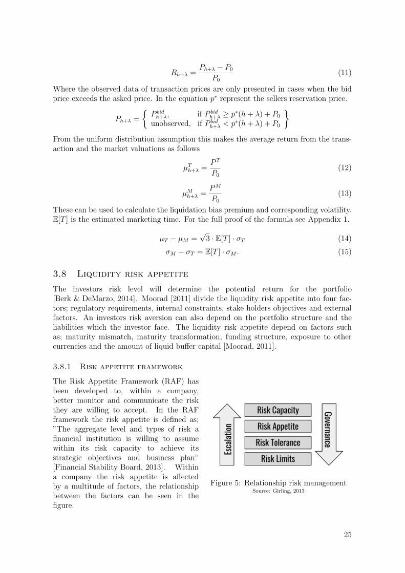
Rh+� =
Ph+� � P0
P0(11)
Where the observed data of transaction prices are only presented in cases when the bid
price exceeds the asked price. In the equation p⇤ represent the sellers reservation price.
Ph+� =
⇢P bidh+�, if P bid
h+� � p⇤(h+ �) + P0
unobserved, if P bidh+� < p⇤(h+ �) + P0
�
From the uniform distribution assumption this makes the average return from the trans-
action and the market valuations as follows
µTh+� =
P T
P0(12)
µMh+� =
PM
P0(13)
These can be used to calculate the liquidation bias premium and corresponding volatility.
E[T ] is the estimated marketing time. For the full proof of the formula see Appendix 1.
µT � µM =
p3 · E[T ] · �T (14)
�M � �T = E[T ] · �M . (15)
3.8 Liquidity risk appetite
The investors risk level will determine the potential return for the portfolio
[Berk & DeMarzo, 2014]. Moorad [2011] divide the liquidity risk appetite into four fac-
tors; regulatory requirements, internal constraints, stake holders objectives and external
factors. An investors risk aversion can also depend on the portfolio structure and the
liabilities which the investor face. The liquidity risk appetite depend on factors such
as; maturity mismatch, maturity transformation, funding structure, exposure to other
currencies and the amount of liquid bu↵er capital [Moorad, 2011].
3.8.1 Risk appetite framework
Figure 5: Relationship risk management
Source: Girling, 2013
The Risk Appetite Framework (RAF) has
been developed to, within a company,
better monitor and communicate the risk
they are willing to accept. In the RAF
framework the risk appetite is defined as;
”The aggregate level and types of risk a
financial institution is willing to assume
within its risk capacity to achieve its
strategic objectives and business plan”
[Financial Stability Board, 2013]. Within
a company the risk appetite is a↵ected
by a multitude of factors, the relationship
between the factors can be seen in the
figure.
25
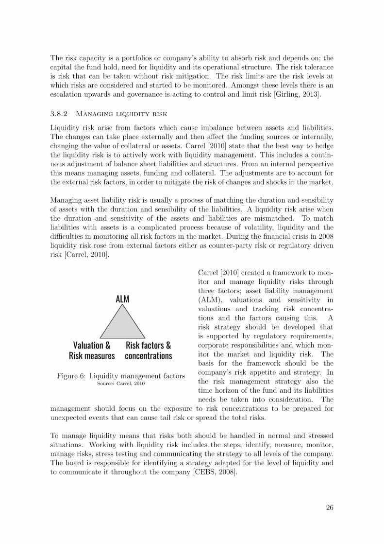
The risk capacity is a portfolios or company’s ability to absorb risk and depends on; the
capital the fund hold, need for liquidity and its operational structure. The risk tolerance
is risk that can be taken without risk mitigation. The risk limits are the risk levels at
which risks are considered and started to be monitored. Amongst these levels there is an
escalation upwards and governance is acting to control and limit risk [Girling, 2013].
3.8.2 Managing liquidity risk
Liquidity risk arise from factors which cause imbalance between assets and liabilities.
The changes can take place externally and then a↵ect the funding sources or internally,
changing the value of collateral or assets. Carrel [2010] state that the best way to hedge
the liquidity risk is to actively work with liquidity management. This includes a contin-
uous adjustment of balance sheet liabilities and structures. From an internal perspective
this means managing assets, funding and collateral. The adjustments are to account for
the external risk factors, in order to mitigate the risk of changes and shocks in the market.
Managing asset liability risk is usually a process of matching the duration and sensibility
of assets with the duration and sensibility of the liabilities. A liquidity risk arise when
the duration and sensitivity of the assets and liabilities are mismatched. To match
liabilities with assets is a complicated process because of volatility, liquidity and the
di�culties in monitoring all risk factors in the market. During the financial crisis in 2008
liquidity risk rose from external factors either as counter-party risk or regulatory driven
risk [Carrel, 2010].
Figure 6: Liquidity management factors
Source: Carrel, 2010
Carrel [2010] created a framework to mon-
itor and manage liquidity risks through
three factors; asset liability management
(ALM), valuations and sensitivity in
valuations and tracking risk concentra-
tions and the factors causing this. A
risk strategy should be developed that
is supported by regulatory requirements,
corporate responsibilities and which mon-
itor the market and liquidity risk. The
basis for the framework should be the
company’s risk appetite and strategy. In
the risk management strategy also the
time horizon of the fund and its liabilities
needs be taken into consideration. The
management should focus on the exposure to risk concentrations to be prepared for
unexpected events that can cause tail risk or spread the total risks.
To manage liquidity means that risks both should be handled in normal and stressed
situations. Working with liquidity risk includes the steps; identify, measure, monitor,
manage risks, stress testing and communicating the strategy to all levels of the company.
The board is responsible for identifying a strategy adapted for the level of liquidity and
to communicate it throughout the company [CEBS, 2008].
26

4 Results
In this section the findings from the empirical and quantitative study are presented. Thisincludes; specifying di↵erent types of real estate and their characteristics, risks withindi↵erent objects, performance measures for real estate and quantifications of de-smoothing,transaction risk and liquidation.
4.1 Real estate investments
All interview participants stated that real estate has historically generated a good risk
adjusted return. The historical return from real estate has been good, even compared
to stocks. The historically obtained risk measure of volatility have been low, from the
available data it is found that in privately owned real estate the standard deviation has
been below 8% per year [Valueguard, 2011] compared to stocks which has had a standard
deviation of about 17% over the same period. Despite the return not being as good as
small cap stocks the lower risk makes real estate having beneficial risk adjusted return
[Gavel, 2017], [Fransson, 2017].
The risk adjusted return is not the only reason to invest in real estate; from the interviews
it was also found that investors saw value in owning a real asset [Skogestig, 2017]. Real
estate is also an attractive investment since it generates a stable cash flow and not only is
dependent on the end value [Skogestig, 2017]. When real estate is bought this is typically
to get the direct cash flow, which mainly come from rents paid [Salen Broman, 2017].
Other advantages includes di↵erentiation to the portfolio as real estate investments are
subject to other risk factors than stocks [Brodin, 2017] but at the same time is a nat-
urally hedge against inflation [Gavel, 2017]. Real estate is also an illiquid investment
[Marcato, 2017].
4.1.1 Illiquidity
During the interviews the general opinion on liquidity risk was that this is present in
real estate investments. Most interview participants stated that this is a risk they were
willing to take in compensation for the liquidity premium they expect to get from real
estate assets. Most interview participants believe there is a liquidity premium in the
Swedish real estate market, but no one had any quantitative estimate on the size of this
premium. A few were skeptical and stated that the liquidity premium is a di↵use term
which is hard to quantify [Lekander, 2017], [Fransson, 2017]. As an example Fransson
[2017] gave was; a company which is bought out from the public market become less liquidas it exits the market. On the other hand the action of removing the company from themarket and therefore becoming more illiquid is not expected to create a higher yield initself. The example was used to describe the liquidity premium puzzle.
The general fear of illiquidity is limited due to the long investment horizons the investors
included in this study have. The investors are knowledgeable about their upcoming cash
flows and have a good prognosis with regards to these cash flows [Salen Broman, 2017].
The investors also have a large section of their assets in more liquid assets, this give the
investors the possibility of taking on some more illiquid investments [Cameras, 2017].
On the other hand some of the investors were careful and monitored their portfolios
liquidity carefully. An example of this is AP3 which internally have limited the
27

amount they may allocate towards illiquid assets to 25% of their total assets. This
limitation was to prevent problems that could arise with liquidity, if the section of
illiquid assets become to large [Hellstrom, 2017]. AP1 on the other hand, which has
about 20% allocated to illiquid assets stated that from a liquidity perspective they
could increase the section of illiquid assets to about 50% but that this level of liq-
uidity would impact the diversification in the portfolio in a negative way [Angberg, 2017].
The fact that institutional investors are aware that properties can take time to sell and
markets could fall decreases the e↵ects a potential liquidity crisis would have on their
portfolio. The main risk with illiquidity is when illiquidty arise where it is not expected.
An example of this was during the financial crisis when Lehman brothers went bankrupt
[Brodin, 2017]. During an interview Brodin [2017] said: ”When you thought you had
invested in something liquid and then it proved not to be. Here you know it is not”,
referring to real estate. In the interviews it was also brought up that the level of liquidity
di↵ers between segments and expressions like ’liquid- and illiquid real estate’ was men-
tioned in some interviews. The degree of liquidity also di↵er between objects, not only
between asset classes [Salen Broman, 2017].
4.2 The different sectors of real estate
When talking about real estate it is important to understand what type of real estate
that is being discussed, because of the di↵erent characteristics in the di↵erent type of real
estate. The IPD-data classify real estate into four main groups; retail, o�ce, residential
and industrial [MSCI, 2016]. MSCI [2016] also have smaller real estate classifications such
as hotels and other but these have not been included in this study. Di↵erent types of
real estate have di↵erent characteristics in terms of risk and return [Gavel, 2017] and also
how real estate is invested in will impact the assets risk - return profile [Brodin, 2017].
From the interviews we found that regarding direct real estate the highest potential
return comes from investments in commercial real estate, given good timing of the market
cycle [Gavel, 2017]. To commercial real estate industrial, retail and o�ces are included
[MSCI, 2016]. Residential real estate is more independent of the market as a place to
live is always needed [Brodin, 2017], [Salen Broman, 2017]. Residential real estate have
had the strongest historical development with value increases of up to 40% per year in
nominal terms in the best years since 1987 [IPD, 2013].
28
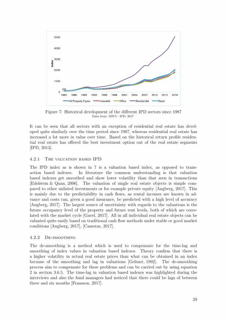
Figure 7: Historical development of the di↵erent IPD sectors since 1987
Data from: MSCI - IPD, 2017
It can be seen that all sectors with an exception of residential real estate has devel-
oped quite similarly over the time period since 1987, whereas residential real estate has
increased a lot more in value over time. Based on the historical return profile residen-
tial real estate has o↵ered the best investment option out of the real estate segments
[IPD, 2013].
4.2.1 The valuation based IPD
The IPD index as is shown in 7 is a valuation based index, as opposed to trans-
action based indexes. In literature the common understanding is that valuation
based indexes get smoothed and show lower volatility than that seen in transactions
[Edelstein & Quan, 2006]. The valuation of single real estate objects is simple com-
pared to other unlisted investments or for example private equity [Angberg, 2017]. This
is mainly due to the predictability in cash flows, as rental incomes are known in ad-
vance and costs can, given a good insurance, be predicted with a high level of accuracy
[Angberg, 2017]. The largest source of uncertainty with regards to the valuations is the
future occupancy level of the property and future rent levels, both of which are corre-
lated with the market cycle [Gavel, 2017]. All in all individual real estate objects can be
valuated quite easily based on traditional cash flow methods under stable or good market
conditions [Angberg, 2017], [Cameras, 2017].
4.2.2 De-smoothing
The de-smoothing is a method which is used to compensate for the time-lag and
smoothing of index values in valuation based indexes. Theory confirm that there is
a higher volatility in actual real estate prices than what can be obtained in an index
because of the smoothing and lag in valuations [Geltner, 1992]. The de-smoothing
process aim to compensate for these problems and can be carried out by using equation
2 in section 3.6.5. The time-lag in valuation based indexes was highlighted during the
interviews and also the fund managers had noticed that there could be lags of between
three and six months [Fransson, 2017].
29
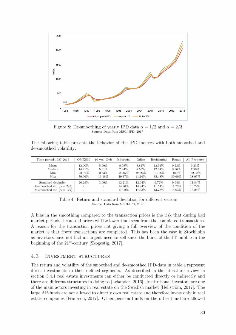
Figure 8: De-smoothing of yearly IPD data ↵ = 1/2 and ↵ = 2/3Source: Data from MSCI-IPD, 2017
The following table presents the behavior of the IPD indexes with both smoothed and
de-smoothed volatility:
Time period 1987-2016 OMXS30 10 yrs. Gvb Industrial O�ce Residential Retail All Property
Mean 12.00% 5.90% 9.08% 8.81% 12.51% 9.23% 9.23%Median 14.21% 5.01% 7.84% 8.53% 12.04% 8.96% 7.96%Min -41.74% 0.53% -20.87% -25.23% -13.18% -18.5% -22.98%Max 70.96% 13.18% 40.37% 41.16% 35.48% 30.69% 38.05%
Standard deviation 26.29% 3.60% 12.21% 12.94% 9.72% 9.94% 11.84%De-smoothed std (↵ = 2/3) - - 14.26% 14.94% 11.54% 11.72% 13.72%De-smoothed std (↵ = 1/2) - - 17.02% 17.63% 13.78% 14.03% 16.24%
Table 4: Return and standard deviation for di↵erent sectors
Source: Data from MSCI-IPD, 2017
A bias in the smoothing compared to the transaction prices is the risk that during bad
market periods the actual prices will be lower than seen from the completed transactions.
A reason for the transaction prices not giving a full overview of the condition of the
market is that fewer transactions are completed. This has been the case in Stockholm
as investors have not had an urgent need to sell since the burst of the IT-bubble in the
beginning of the 21
st-century [Skogestig, 2017].
4.3 Investment structures
The return and volatility of the smoothed and de-smoothed IPD-data in table 4 represent
direct investments in their defined segments. As described in the literature review in
section 3.4.1 real estate investments can either be conducted directly or indirectly and
there are di↵erent structures in doing so [Lekander, 2016]. Institutional investors are one
of the main actors investing in real estate on the Swedish market [Hellstrom, 2017]. The
large AP-funds are not allowed to directly own real estate and therefore invest only in real
estate companies [Fransson, 2017]. Other pension funds on the other hand are allowed
30

to own real estate directly but this may not be done using leverage [Evander, 2017],
[Salen Broman, 2017].
4.3.1 Characteristics
Figure 9: Characteristics of real estate
From the interviews it was found that in-
vestors are expecting between 4-8% return
annually for directly owned real estate.
The expected return is dependent on the
object and its characteristics and location
[Salen Broman, 2017]. Considering a Core
real estate object the expected return is
just a few percent per year and this is con-
sidered as a stable investment which have
characteristics similar to that of a bond.
Opportunistic real estate investments on
the other hand behave more like stocks and
have higher risk but also require a higher
premium to compensate for the risk [Salen Broman, 2017]. Also the level of liquidity can
be connected to the location as seen from the position in the matrix shown in the figure.
4.4 Liquidity risk for single properties
The liquidity of objects vary depending on the characteristics and location of the object
[Salen Broman, 2017]. During the interviews the term ’liquid and illiquid properties’
came up. As liquid real estate objects are Core properties in Central Business Districts
(CBD) considered [Cameras, 2017]. Core objects that have a central or unique location
are liquid, as in terms of that buyers can be found, even in times of poor market liquidity
[Salen Broman, 2017]. The number of potential buyers for an object and the location of
the building play an important role for the liquidity of the object [Gavel, 2017]. ”There
is only one Biblioteksgatan in Stockholm” [Salen Broman, 2017]. In urban, crowded
areas, it is hard to construct new buildings to compete with the existing ones. This
can be compared to for example warehouses on the countryside where if someone needs
a new warehouse a new can be built as there is not usually a problem to get land
[Nystrom, 2017]. The location is a factor a↵ecting the ability to sell and make a profit
for an investment [Salen Broman, 2017].
Other than the location the way the building is used impact the liquidity of the object.
Residential real estate is the most stable and liquid form of real estate investment ac-
cording to all interviews. This is explained by the demand for housing in urban areas in
Sweden, regardless of the condition of the market. The prices will fluctuate but in the
long run the value of residential real estate is expected to rise with inflation [Gavel, 2017].
Commercial real estate, for example retail space, is more dependent on the market cycles
[Gavel, 2017]. Retail is followed by o�ces and ware houses when it comes to risk. These
two categories have a risk highly dependent on the property, its location and the tenants
[Cameras, 2017].
31
4.4.1 Information imbalance
Some of the investors selected for the interviews only invest in new properties as for
older ones there is direct risks with the object such that renovations or repairs may be
required. The greater the need for large capital investments the more opportunistic is
the object, as the potential up- and downside increase [Salen Broman, 2017]. The risk
of unexpected surprises in older properties is reduced by the due diligence process that
is conducted on all larger objects before they are traded [Skogestig, 2017]. Reparation
cost is a moderate risk for owners and institutions as the costs usually can be put on
the part using the building through fees or increased rents. Because of this the risk of
renovation cost is a moderate risk as the costs usually can be conveyed on to the tenants
[Salen Broman, 2017].
4.4.2 Vacancies
Almost all of the cash flow from real estate comes from rents, either from private persons
or companies [Skogestig, 2017]. From the interviews a major risk with real estate was
identified as long time vacancies. In attractive locations in Sweden this has not been
an issue since the burst of the IT-bubble in the early years of the new century as the
demand for space has exceeded the supply as the market has gone up [Skogestig, 2017].
The rent levels are often determined for the duration of the contract, but depending of
the conditions in the market once the contract runs out the rent level may change. The
occupancy level on the other hand is more directly correlated with the performance of
the person or companies renting and then in turn the market cycle. With higher levels
of vacancies the cash flow for the object decrease, for this to have a large impact on the
over all portfolio return there needs to be quite drastic changes in the market condition
[Bergstrom & Hansen Vikstrom, 2017].
In new projects there is always a risk that there will be no or low demand for the
property once built. This is further increased by the time it takes to complete the project
and that it thereby is likely that market conditions change during the building process
[Salen Broman, 2017]. In order to combat this issue it is common that objects are built
to pre-determined tenants. In residential real estate it is more common that the projects
are built on speculation, but due to the law regarding utility rent in Sweden almost all
residential real estate built for the rental market in Stockholm will be fully subscripted
even before construction start [Gavel, 2017].
It may be harder to find tenants for commercial real estate. This risk is often me-
diated through rarely building o�ces on speculation and rather building to a known
customer, a pre-rented level of about 60-70% is often enough to in the current market
reach a break-even level for the project, given that the budget for the project holds
[Bergstrom & Hansen Vikstrom, 2017]. This is the most common practice when it comes
to o�ce buildings. When it comes to even more specific projects, which is common
in logistic or industrial properties the level of speculation in projects is even lower
[Gavel, 2017].
Some of the risk with vacancies can be removed through decreasing rent, and in this way
keep tenants [Skogestig, 2017]. If there are vacancies there will be lower rental incomes
as well as the current rental holders will have a better position for negotiating their rents
32
[Bergstrom & Hansen Vikstrom, 2017]. The risk of vacancies can also be decreased by
di↵erentiation as the number of tenants increases. A building where the rent is payed
by only one company or person carries a higher risk of vacancies than a building with
many tenants. This could for example be the case with industrial buildings which only
one company is using [Salen Broman, 2017].
4.5 Real estate and the economic cycle
The risk of vacancies presented in section 4.4.2 is correlated with the market cycle and
can therefore be considered to be a market risk. During falling markets or recessions
more objects become vacant [Skogestig, 2017]. Real estate is sensitive to changes in the
market cycle with varying exposure depending on segment and investment structure
[Gavel, 2017]. Commercial real estate as industrial-, o�ce- and retail real estate is more
volatile than residential real estate. People need a place to live regardless of the state of
the market cycle [Brodin, 2017]. The commercial sectors dependent on the results from
the companies renting which is why they tend to be more a↵ected by the market cycle
[Cameras, 2017].
How the real estate investments move in relation to the market is also dependent on
the selected structure for the investment. Through investing in real estate or real es-
tate companies on the open market the investor faces a lower level of liquidity risk
[Salen Broman, 2017]. Assets that are publicly traded will behave more like the mar-
ket and have a higher correlation to the market. Funds traded o↵ the market and other
direct real estate investments follows the real estate market better [Gavel, 2017]. Invest-
ing in real estate stocks, the development is more like stocks and less like the underlying
and have a higher volatility than other real estate assets. This can for example be seen
in the value of noted companies such as Fabege, which is a real estate firm investing in
o�ces in the Stockholm area. Fabeges historical volatility is 15% which is comparatively
higher than the volatility of real estate indexes. From interviews we found that the com-
paratively higher volatility was explained by stocks in public real estate firms also being
subject to reactions in the market and thereby subject to market volatility [Ang, 2014],
[Evander, 2017].
4.5.1 Diversification
From the interviews it was found that another main reasons to include real estate in
a portfolio was because of the beneficial correlation between real estate and stocks or
bonds. When building a portfolio it is desirable to have a low correlation between the
assets to minimize the risk in the portfolio without giving up to much of the potential
return [Berk & DeMarzo, 2014].
Correlation between stocks and real estate vary drastically over time, as seen in the graph
below. In this graph the rolling 12 month correlation between HOX-All Sweden to bonds
and stocks is shown. The index RXVX represents Swedish treasury bills and OMXS30 is
the index for the 30 largest stocks on the Swedish stock market.
33
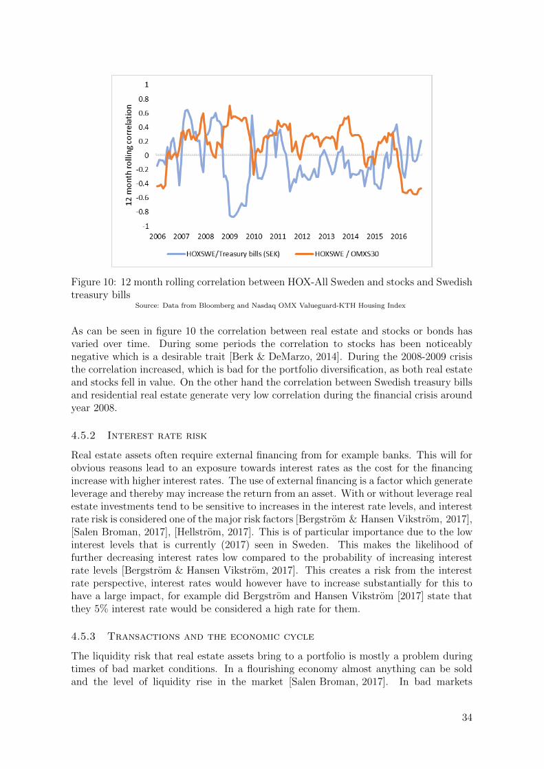
Figure 10: 12 month rolling correlation between HOX-All Sweden and stocks and Swedish
treasury bills
Source: Data from Bloomberg and Nasdaq OMX Valueguard-KTH Housing Index
As can be seen in figure 10 the correlation between real estate and stocks or bonds has
varied over time. During some periods the correlation to stocks has been noticeably
negative which is a desirable trait [Berk & DeMarzo, 2014]. During the 2008-2009 crisis
the correlation increased, which is bad for the portfolio diversification, as both real estate
and stocks fell in value. On the other hand the correlation between Swedish treasury bills
and residential real estate generate very low correlation during the financial crisis around
year 2008.
4.5.2 Interest rate risk
Real estate assets often require external financing from for example banks. This will for
obvious reasons lead to an exposure towards interest rates as the cost for the financing
increase with higher interest rates. The use of external financing is a factor which generate
leverage and thereby may increase the return from an asset. With or without leverage real
estate investments tend to be sensitive to increases in the interest rate levels, and interest
rate risk is considered one of the major risk factors [Bergstrom & Hansen Vikstrom, 2017],
[Salen Broman, 2017], [Hellstrom, 2017]. This is of particular importance due to the low
interest levels that is currently (2017) seen in Sweden. This makes the likelihood of
further decreasing interest rates low compared to the probability of increasing interest
rate levels [Bergstrom & Hansen Vikstrom, 2017]. This creates a risk from the interest
rate perspective, interest rates would however have to increase substantially for this to
have a large impact, for example did Bergstrom and Hansen Vikstrom [2017] state that
they 5% interest rate would be considered a high rate for them.
4.5.3 Transactions and the economic cycle
The liquidity risk that real estate assets bring to a portfolio is mostly a problem during
times of bad market conditions. In a flourishing economy almost anything can be sold
and the level of liquidity rise in the market [Salen Broman, 2017]. In bad markets
34

no or few transactions are completed and there is then no market to trade less liquid
investments as for example real estate [Skogestig, 2017]. In a diminishing market most
pressure is on actors which have taken on bad investments or taken high risks with
potentially high leverage [Gavel, 2017]. On the Swedish market, actors are prepared
for periodical drops in real estate investments. The actors with large quantities of
real estate are large with stable balance sheets and long investment horizons. Their
stable balance sheets decreases their potential need to sell during negative market times
[Hellstrom, 2017].
Another aspect that Gavel [2017] brought up was that banks and companies do not
want the valuations to go down on properties and there is therefore a risk of investors
exchanging properties between investors to show up higher prices then the actual market
values. This could pose a valuation risk as transactions shown could not be trusted.
The most common way to value a portfolio is to use a benchmark index, and use this
for comparison to which statistical methods can be applied and values under varying
market conditions extracted. These indexes are usually valuation based and updated
on a annual or quarterly basis which may further contribute to the problem with time
lag or smoothed valuations. The indexes which can be used for estimating the value
of the portfolios is not always representative for the objects that are in the portfolio
[Angberg, 2017]. More transactions in comparable objects would make valuations and
transactions easier to validate, but because of the limited stock of objects and fewer
transactions during recession this data is not always available [Skogestig, 2017].
4.5.4 Lock in effect
A scenario with a falling market where no or few transactions take place may cause
worries for a lock in. According to Brodin [2017] investors fear to get locked into an
asset and thereby have limited ability to invest in opportunities that may arise in the
future. This risk is large with real estate assets due to the long investment horizon of this
asset class. Making bad investment decisions are always a risk but the alternative to not
make any investments and wait for an opportunity is not an option [Brodin, 2017]. One
way of handling the lock in e↵ect when buying real estate as structured products with a
duration, suggested by Brodin [2017], is to buy small portions yearly and then eventually
create a portfolio with possibility to exit more frequently.
4.6 Transaction risk
The transaction risk which is part of the liquidity risk can be calculated using the ex-ante
formula presented in section 3.6.7. In table 7 di↵erent scenarios for the scaling factor
for liquidity is shown. This is dependent on the expected holding period and transaction
period.
4.6.1 Transaction and holding period
To decide the transaction period Hordijk and Teubens [2008] steps in the transaction
process described in section 3.6 can be used to give a better estimation of the time and
compare answers from interviews with what is used in the formula. The transaction
period used in the ex-ante formula is measured from the time of a decision to sell an asset
to the completion of the trade. This means that the transaction period does not only
35

include the time it takes to transfer the cash but also the pre-marketing-, marketing-
and due diligence period.
From the interviews the time from the point of getting in contact with a potential buyer
to the completion of the trade can be estimated to take between three to six months
for direct real estate investments. In table 5 the answers from respective interview has
been summarized. The interval is close to that found by Hordijk and Teuben [2008]
who found the transaction period in Britain lasts between two and six months. This is
under the presumption that the trade is successful. The success of the trade depend
on the market cycle and not all trades are successful and an asset can instead be
removed from the market. The unsuccessful transactions can not be seen in the statistics
[Cameras, 2017]. For successful trades the time it takes to sell an asset is dependent on
the number of potential buyers for the objects given the present market conditions and
the characteristics of the object. For larger properties more time is usually invested to
make an interesting case and attract more buyers which means that the transaction time
is usually longer for larger objects [Skogestig, 2017].
The following table represent the summarized answers regarding expected transaction
and holding periods from the interview participants:
Name Company Holding period Transaction periodJ. Skogestig Vasakronan Infinity 3-6 monthsB. Hellstrom AP3 Infinity 3 monthsR. Gavel SEB 8 yrs 6 months
F. Salen Broman SEB Long 2-3 monthsM. Cameras AMF Infinity >3 months, <1 yrA. Bergstrom Fabege Infinity -M. Angberg AP1 Infinity -T. Fransson AP4 Long 6 monthsO. Nystrom AP4 Long 6 monthsA.Evander FPK Infinity 3-6 months
Table 5: Summary of investment assumptions
Most interview participants claim to have no end date for real estate investments
and assume that these will be in the portfolios forever. When valuating proper-
ties usually a ten year time horizon is used even though no fixed time horizon is
decided before hand [Skogestig, 2017]. However, some of the interview participants
had fixed end dates for their real estate investments due to the structures of their
funds. Pension funds have long time horizons in their investments as liabilities are far
into the future [Hellstrom, 2017]. Out of the investors with limited horizons, one was
a real estate fund with duration of eight years, the other one a pension fund closing down.
From the institutionally owned properties represented in the IPD database the results
for the implied holding period can be seen in table 6. The average holding period for
all properties is 12 years. O�ces and retail have the highest average implied holding
period with 16 years. During the period between 2005 and 2012 very few trades were
completed in all categories. In 2008 no institutionally owned real estate included in the
IPD database was traded. It can be seen that before the period 2005-2012 real estate
36

were held for shorter time periods than what is implied during the last four years.
Table 6: Implied holding period
Year 01 02 03 04 05 06 07 08 09 10 11 12 13 14 15 16 Mean
All properties 4 7 5 10 9 9 10 17 14 19 14 21 13 10 16 12Industrial 5 4 6 8 32 19 14 23 14O�ce 5 9 6 11 29 15 24 25 16
Residential 4 6 4 8 19 29 22 13Retail 5 9 6 11 29 15 24 25 16
*The blank spaces are due to the the implied formula (3) of holding periods. During years with no sales the impliedholding period can not be calculated, as this is the denominator in the formula.
4.6.2 Ex-ante variance HOX
For the initial calculation of ex-ante variance HOX-index was used, as HOX is transaction
based no de-smoothing had to be conducted. The HOX-index is available on monthly
basis from January 2005 until December 2016 for this study. The ex-ante scaling below is
based on monthly transaction period and holding period, the mean and variance factors
in the input is also in monthly form.
Table 7: Ex-ante scaling HOX 2005-2016
Holding period
Transaction period 1 6 12 24 60 120 182
1 1.066 1.019 1.010 1.005 1.002 1.001 1.0013 1.296 1.131 1.079 1.044 1.019 1.010 1.0066 1.676 1.394 1.263 1.158 1.072 1.038 1.02510 2.195 1.821 1.597 1.387 1.188 1.101 1.06812 2.456 2.051 1.789 1.526 1.263 1.143 1.09815 2.848 2.408 2.095 1.758 1.394 1.219 1.15020 3.503 3.022 2.643 2.195 1.657 1.376 1.26024 4.028 3.523 3.103 2.577 1.901 1.526 1.36760 8.756 8.169 7.571 6.633 4.943 3.629 2.955
The scaling factor in the table presents the transaction risk which is part of the illiquidity
risk and can not be measured using volatility. To better estimate the risk of real estate
investments the factor should therefore be used to multiple the obtained variance. In
table 7 it can be seen that the ex-ante scaling factor increase as the transaction period
in proportion to the holding period increases.
In the table below a summary of the 6 months transaction period 120 months holding
period for each division of the HOX-index can be seen. The use of six months transac-
tion period is selected to represent the approximate transaction period found from the
interviews, the 120 month holding period as benchmark was selected to match the calcu-
lation horizon of Vasakronan. The table is based on annual return and annual standard
deviation.
37

Table 8: Summary of return and volatility
Index Annual return St. dev Scaling factor Scaled St. dev Sharpe ratio
All Sweden 7.3% 5.6% 1.038 5.7% 0.827Flats Sweden 9.8% 6.2% 1.054 6.4% 1.130
Flats Stockholm 9.6% 7.2% 1.038 7.4% 0.954Flats Gothenburg 10.7% 7.0% 1.050 7.2% 1.133
Flats Malmo 7.8% 8.0% 1.021 8.0% 0.654Flats other cities 10.3% 5.9% 1.065 6.1% 1.262Houses Sweden 6.4% 6.2% 1.023 6.3% 0.605
Houses Stockholm 7.1% 7.4% 1.020 7.5% 0.606Houses Gothenburg 7.0% 7.7% 1.018 7.8% 0.570
Houses Malmo 5.1% 7.9% 1.009 7.9% 0.318Houses other cities 6.1% 7.1% 1.017 7.1% 0.495
SBX 11.9% 17.0% - - 0.551OMXS 30 7.5% 17.3% - - 0.285
10 yrs. Gvt. Bond 2.5% 1.2% - - -
As can be seen in the table above, residential real estate has over the last 11 years outper-
formed OMXS30 in terms of Sharpe ratio, this is mainly explained by the higher volatility
associated with stocks rather than real estate as the two asset classes has quite similar
average annual return. Over the period flats in other cities than the three metropoli-
tan areas in Sweden have given the highest risk adjusted return after adjusting for the
transaction period risk. In this measure it should be noted that only successful trades
are reported and there are rural areas where there is hard to find buyers which could be
a potential bias for this measurement. Single family homes in Malmo yielded the lowest
risk adjusted return after transaction period risk was included, the risk adjusted return
is however still greater than that of OMXS30.
4.6.3 Ex-ante variance of IPD index All Property
The data from the IPD:s category of ’All property’ in general give low scaling factors.
The scaling factors in the table shows that the volatility should be increased by a factor
of 1.013 assuming a holding period of ten years and a transaction time of six months,
if smoothed data is used. In the first two tables original data, prior to de-smoothing is
used. In the two following tables de-smoothed data with ↵ = 0.5 has been used.
38

Table 9: Ex-ante scaling IPD All Property 1987-2016
Holding period
Transaction period 1 6 12 24 60 120 182
1 1.023 1.007 1.004 1.002 1.001 1.000 1.000
3 1.105 1.047 1.028 1.016 1.007 1.003 1.002
6 1.240 1.140 1.093 1.056 1.025 1.013 1.009
10 1.424 1.292 1.212 1.137 1.067 1.036 1.024
12 1.517 1.373 1.280 1.187 1.093 1.051 1.035
15 1.656 1.500 1.389 1.269 1.140 1.078 1.053
20 1.889 1.718 1.583 1.424 1.233 1.133 1.092
24 2.075 1.896 1.747 1.560 1.320 1.187 1.130
60 3.754 3.545 3.333 3.000 2.400 1.933 1.694
Just like in table 7 the results in table 9 show that the longer the expected holding
period the smaller the ex-ante scaling factor and the longer the expected transaction
period the larger the ex-ante scaling factor. This means that the longer the transac-
tion period in comparison to the holding period the greater the transaction period risk
[Bond & Huang, 2004].
Table 10: Summary of return and volatility, years 1987-2016
Index Annual return St. dev Scale factor Scaled st.dev Scaled Sharpe ratio
All property 9.2% 11.8% 1.013 12.0% 0.278Industrial 9.1% 12.2% 1.020 12.4% 0.255O�ce 8.8% 12.9% 1.016 13.1% 0.221
Residential 12.5% 9.7% 1.046 10.2% 0.650Retail 9.2% 9.9% 1.012 10.1% 0.331
OMXS30 12.0% 26.3% - - 0.23210 Y Gvt Bond 5.9% 3.6% - -
In the table above it can be seen that all Sharpe ratios are of about the same scale for
the smoothed data and OMXS30, with an exception of residential real estate. As Sharpe
ratio is a measurement of risk adjusted return, having Sharpe ratios corresponding to
that of stocks should be an indicator that the risk taken when investing in an asset is
rewarded with the current level of average return [Sharpe, 1964].
39
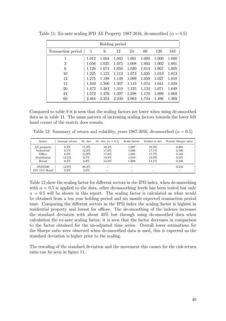
Table 11: Ex-ante scaling IPD All Property 1987-2016, de-smoothed (↵ = 0.5)
Holding period
Transaction period 1 6 12 24 60 120 182
1 1.012 1.004 1.002 1.001 1.000 1.000 1.0003 1.056 1.025 1.015 1.008 1.004 1.002 1.0016 1.128 1.074 1.050 1.030 1.014 1.007 1.00510 1.225 1.155 1.113 1.073 1.035 1.019 1.01312 1.275 1.198 1.149 1.099 1.050 1.027 1.01815 1.349 1.266 1.207 1.143 1.074 1.041 1.02820 1.472 1.382 1.310 1.225 1.124 1.071 1.04924 1.572 1.476 1.397 1.298 1.170 1.099 1.06960 2.464 2.353 2.240 2.063 1.744 1.496 1.369
Compared to table 9 it is seen that the scaling factors are lower when using de-smoothed
data as in table 11. The same pattern of increasing scaling factors towards the lower left
hand corner of the matrix does remain.
Table 12: Summary of return and volatility, years 1987-2016, de-smoothed (↵ = 0.5)
Index Annual return St. dev St. dev (↵ = 0.5) Scale factor Scaled st.dev Scaled Sharpe ratio
All property 9.2% 11.8% 16.2% 1.007 16.3% 0.204Industrial 9.1% 12.2% 17.0% 1.006 17.1% 0.186O�ce 8.8% 12.9% 17.6% 1.005 17.7% 0.165
Residential 12.5% 9.7% 13.8% 1.018 13.9% 0.475Retail 9.2% 9.9% 14.0% 1.009 14.1% 0.236
OMXS30 12.0% 26.3% - - - 0.23210Y Gvt Bond 5.9% 3.6% - - - -
Table 12 show the scaling factor for di↵erent sectors in the IPD index, when de-smoothing
with ↵ = 0.5 is applied to the data, other de-smoothing levels has been tested but only
↵ = 0.5 will be shown in this report. The scaling factor is calculated as what would
be obtained from a ten year holding period and six month expected transaction period
time. Comparing the di↵erent sectors in the IPD index the scaling factor is highest in
residential property and lowest for o�ces. The de-smoothing of the indexes increases
the standard deviation with about 40% but through using de-smoothed data when
calculation the ex-ante scaling factor, it is seen that the factor decreases in comparison
to the factor obtained for the un-adjusted time series. Overall lower estimations for
the Sharpe ratio were observed when de-smoothed data is used, this is expected as the
standard deviation is higher prior to the scaling.
The rescaling of the standard deviation and the movement this causes for the risk-return
ratio can be seen in figure 11.
40

Figure 11: Risk return movement for IPD data
Source: Data from Bloomberg and IPD, 2017
4.6.4 Ex-ante variance, IPD and HOX comparison
It needs to be noted that the IPD-data is based on the time period 1987 - 2016 whereas
the HOX index is available for the time period 2005 - 2016. It should also be noted that
the volatility scaling for the category of all property is used for IPD and the HOX index
includes only residential real estate. These two di↵erences means that comparisons have
to be handled with caution and for this reason no direct comparisons in either graphs or
table are figuring in this study. Instead a more general discussions is carried out of the
findings.
In the figure below the risk and return profile, scaled for de-smoothing and ex-ante vari-
ance for IPD data compared to OMX30 and government bond returns can be seen.
41

Figure 12: Risk return profile for scaled IPD
Source: Data from Bloomberg and IPD, 2017
As can be seen in figure 12 the risk return profile seem to fit quite well in the risk-return
spectrum between stocks and bonds. This does not hold for HOX-index as can be seen
in the figure 13, it can also be seen that OMXS30 has had a fairly low return compared
to Stockholm Benchmark Index (SBX) which also include smaller stocks.
Figure 13: Risk return profile for scaled HOX
Source: Bloomberg and Nasdaq OMX Valueguard-KTH Housing Index, 2017
It is quite noticeable that most of the sub-indexes included in HOX have a risk-return
profile higher than that of OMXS30. This would imply that the risk adjusted return
for investing in residential real estate is higher than that of large cap stocks, however
the risk adjusted return is just slightly higher than that of SBX, which is the Stockholm
benchmark index. Residential real estate in the IPD-data give higher risk adjusted return
than OMXS30. The risk adjusted return after scaling for ex-ante variance is still higher
42
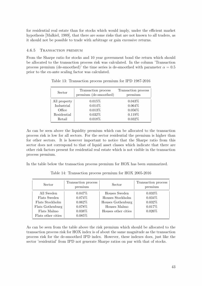
for residential real estate than for stocks which would imply, under the e�cient market
hypothesis [Malkiel, 1989], that there are some risks that are not known to all traders, as
it should not be possible to trade with arbitrage or gain excessive returns.
4.6.5 Transaction premium
From the Sharpe ratio for stocks and 10 year government bond the return which should
be allocated to the transaction process risk was calculated. In the column ’Transaction
process premium (de-smoothed)’ the time series is de-smoothed with parameter ↵ = 0.5prior to the ex-ante scaling factor was calculated.
Table 13: Transaction process premium for IPD 1987-2016
SectorTransaction process
premium (de-smoothed)Transaction process
premium
All property 0.015% 0.043%Industrial 0.014% 0.064%O�ce 0.013% 0.056%
Residential 0.032% 0.119%Retail 0.018% 0.032%
As can be seen above the liquidity premium which can be allocated to the transaction
process risk is low for all sectors. For the sector residential the premium is higher than
for other sectors. It is however important to notice that the Sharpe ratio from this
sector does not correspond to that of liquid asset classes which indicate that there are
other risk factors present for residential real estate which is not visible in the transaction
process premium.
In the table below the transaction process premium for HOX has been summarized.
Table 14: Transaction process premium for HOX 2005-2016
SectorTransaction process
premiumSector
Transaction processpremium
All Sweden 0.047% Houses Sweden 0.033%Flats Sweden 0.074% Houses Stockholm 0.034%
Flats Stockholm 0.062% Houses Gothenburg 0.032%Flats Gothenburg 0.078% Houses Malmo 0.017%
Flats Malmo 0.038% Houses other cities 0.026%Flats other cities 0.085%
As can be seen from the table above the risk premium which should be allocated to the
transaction process risk for HOX index is of about the same magnitude as the transaction
process risk for the de-smoothed IPD index. However, these indexes does, just like the
sector ’residential’ from IPD not generate Sharpe ratios on par with that of stocks.
43

4.7 Time horizon and transaction costs
When considering an investment, the time horizon for the investment is an important
aspect, especially when it comes to assets with high transaction cost such as real estate.
When there are high transaction costs this needs to be accounted for in the pricing and
in the intended holding period. Which follow form the liquidity discount described in
section 3.5. An asset with a lower transaction cost but which is traded more frequently
could in the long run have the same total transaction cost as an investment with a long
holding period and high transaction costs [Lekander, 2017].
In larger real estate objects the transaction cost is relatively fixed no matter of the fi-
nal transaction price. The process of buying or selling costs almost the same for an
equivalent building in a unattractive area with lower value as for an attractive area
[Skogestig, 2017]. This is because of the steps that the transaction process goes through.
For a proper examination of an object decreasing the risk of the trade there are several
steps that have to be gone through. As a buyer these steps include hiring a lawyer,
financial-, technical- and environmental due-diligence, valuations and potentially getting
loan agreements [Gavel, 2017]. Because of the relatively fixed cost independent of the
value of the house the transaction cost can range between 0.5% to 5% for larger transac-
tions [Skogestig, 2017]. Most of these costs are dependent on the need to hire consultants
to help with the transaction, if theses skills are available in-house the transaction cost
from the sellers side can be reduced to just a few basis points, but this in terms increase
the company costs [Bergstrom & Hansen Vikstrom, 2017].
4.8 Forced sales
A situation of forced sales could be caused by; demand for cash to a di↵erent investment,
a drop in value of other asset classes, changes in regulation which the particular fund is
obliged to follow or that a new management has di↵erent views on how to best invest the
capital amongst many factors. Being forced to sell an asset can lead to lower sales price
as fewer actors will have time to act or make the required decisions [Donner et al., 2016],
[Campbell et al., 2011]. A downside with being forced to sell an asset is that it is likely
that the investor will not have su�cient time to market the asset. As seen in the literature
review of section 3.7 the estimated value decrease in a situation of forced sales is between
20 and 30% [Donner et al., 2016]. The total e↵ect of the expected accumulated return is
large if the risk of forced sale is included.
44

Figure 14: Forced sales e↵ect on expected return
In the figure above the expected accumulated return can be seen for two assets with an
annual return of 7.3% which is the historical average return for HOX all Sweden. The
investor has got a risk of fire sale of 2% per year and a cost in case of fire sale of 20% of
the accumulated value at the time of the sale, which is in the lower spectrum of empirical
value decrease [Donner et al., 2016]. These scenarios are based on a general case and
needs to be adjusted depending on the funds risk and structure.
As can be seen in the graph above the risk of fire sale has got a large impact on the
expected return. If the lock in period is 10 years in the set up described above the second
asset is required to generate 8.25% return per year to generate the same expected return
as the asset with no risk of fire sale. However, if the lock in period is 30 years and the
other assumptions the same, the required compensation is 8.87%. This shows that the
risk with fire sale increase with longer expected holding period, given constant annual
risk of fire sale.
4.8.1 Liquidation premium
The need of selling a property immediately can be represented by the liquidation premium
seen as the return bias in the following table. The liquidation bias is the inability of obtain-
ing full market price when a trade has to take place immediately [Lin & Vandell, 2007].
The market return and volatility is what will be obtained by the seller for di↵erent mar-
keting periods. A marketing period of six months would for the seller imply a negative
return of 1% and the liquidation premium is in this case 10.3%.
45
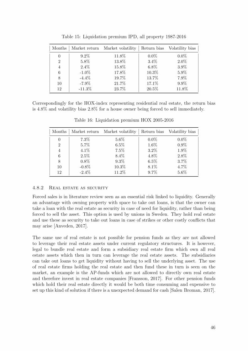
Table 15: Liquidation premium IPD, all property 1987-2016
Months Market return Market volatility Return bias Volatility bias
0 9.2% 11.8% 0.0% 0.0%2 5.8% 13.8% 3.4% 2.0%4 2.4% 15.8% 6.8% 3.9%6 -1.0% 17.8% 10.3% 5.9%8 -4.4% 19.7% 13.7% 7.9%10 -7.9% 21.7% 17.1% 9.9%12 -11.3% 23.7% 20.5% 11.8%
Correspondingly for the HOX-index representing residential real estate, the return bias
is 4.8% and volatility bias 2.8% for a house owner being forced to sell immediately.
Table 16: Liquidation premium HOX 2005-2016
Months Market return Market volatility Return bias Volatility bias
0 7.3% 5.6% 0.0% 0.0%2 5.7% 6.5% 1.6% 0.9%4 4.1% 7.5% 3.2% 1.9%6 2.5% 8.4% 4.8% 2.8%8 0.8% 9.3% 6.5% 3.7%10 -0.8% 10.3% 8.1% 4.7%12 -2.4% 11.2% 9.7% 5.6%
4.8.2 Real estate as security
Forced sales is in literature review seen as an essential risk linked to liquidity. Generally
an advantage with owning property with space to take out loans, is that the owner can
take a loan with the real estate as security in case of need for liquidity, rather than being
forced to sell the asset. This option is used by unions in Sweden. They hold real estate
and use these as security to take out loans in case of strikes or other costly conflicts that
may arise [Anveden, 2017].
The same use of real estate is not possible for pension funds as they are not allowed
to leverage their real estate assets under current regulatory structures. It is however,
legal to bundle real estate and form a subsidiary real estate firm which own all real
estate assets which then in turn can leverage the real estate assets. The subsidiaries
can take out loans to get liquidity without having to sell the underlying asset. The use
of real estate firms holding the real estate and then fund these in turn is seen on the
market, an example is the AP-funds which are not allowed to directly own real estate
and therefore invest in real estate companies [Fransson, 2017]. For other pension funds
which hold their real estate directly it would be both time consuming and expensive to
set up this kind of solution if there is a unexpected demand for cash [Salen Broman, 2017].
46
4.9 Institutional investors inclusion of real estate
There can be di↵erent objectives behind the decision to include real estate in a portfolio.
Depending on the strategy behind including alternative investments also the structure of
the rest of the portfolio needs to be taken into consideration [Brodin, 2017]. The allocation
of real estate di↵ered between the pension funds both in size and structure. Many smaller
institutional investors today have allocations of less than five percent to direct real estate
[Brodin, 2017]. Other funds included also real estate companies and some of the stocks
to the category and then reach an allocation of about 20% [Svensk forsakring, 2017]. A
problem with these numbers is however that the definition of what is included in real
estate vary depending on the fund and there are no clear guidelines on what should be
included in the asset class ’real estate’ [Gustavsson, 2017].
4.9.1 Capital structure and ALM
For institutional investors with long time horizons and known debts at future points,
investors search to find investments with similar performance as time horizons to match
there liability and thereby get a natural hedge. For pension funds part of the dept can
be cash flows 30 or 40 years in the future, future payments are discounted with the
interest rate curve. To hedge the future payment investors want to have products that
follow interests with this long duration, whereas government bonds usually have duration
time of 15 years maximum. This creates a duration risk in the portfolio and investors
are often trying to use interest rates swaps to get a longer duration [Salen Broman, 2017].
Investments with long duration that moves with interest levels are therefore interesting
for pension funds as they o↵er good hedge of the liability. From an ALM perspective there
could be a reason of including real estate investments as these have a long time horizon
and the prices follows the inflation. Investing in Core real estate assets the stable yield
and the lower degree of liquidity risk in comparison to other real estate classes makes it
interesting to act as bonds to gain a stable cash flow [Salen Broman, 2017].
4.9.2 Size matters
Forming an illiquid portfolio takes time and it also requires the portfolio to be of a
certain size for a diversified direct real estate investment [Brodin, 2017]. The sizes of the
funds which hold long time capital vary. The large AP-funds holds way more capital
then the small occupational pension funds, which may have just a fraction of the capital
of the large actors. Through investing in larger lot sizes the transaction costs becomes
a smaller section of the transaction value as most of the transaction cost is fixed in the
majority of transactions [Gavel, 2017].
In order to then gain diversification in the portfolio of real estate, which is important
to reduce the risk in the investment, at least five or six properties in di↵erent locations
should to be included in the portfolio [Gavel, 2017]. The real estate risk is best diversified
geographically than through the spectrum of real estate classes [Brodin, 2017]. To create
a diversified portfolio of between five and six objects, which would be the smallest
number required for a diverse portfolio, you are required an investment of about 2.5billion SEK. For the real estate investments to correspond to 10% of the total diversified
portfolio, this requires the portfolio to hold at least 25 billion SEK worth of assets
47

[Gavel, 2017]. When the portfolio asset reach 25 billion SEK the portfolio is, by Swedish
comparison, no longer a small portfolio [Svensk forsakring, 2017]. If the fund is unable
to own their real estate portfolio directly or through subsidiaries due to size restrictions
an option for getting real estate exposure is to invest in real estate funds. These are
however, limited in their lifetime and by this more exposed to timing risk as they have a
pre-determined end date, and are thereby subject to the market conditions at the end of
the lifetime of the fund [Gavel, 2017].
From the statement that the fund is required to have at least 25 billion SEK in assets in
order to e�ciently invest in direct real estate is not supported by forsakringsbranschens
pensionskassa (FPK), they are a fund with about 14 billion SEK in assets and have a
portfolio of directly owned real estate. In FPK:s opinion they can manage their current
holdings without the concern of size. On the other hand they are currently choosing to
invest in real estate through real estate funds [Evander, 2017]. This would support that
funds of comparatively smaller size is limited in their real estate investments by the large
lot sizes that is bought and sold in the real estate market, but the holding of direct real
estate is not subject to the size of the fund.
As mentioned real estate is a real asset and real estate assets are associated with costs
that are not present in management of financial securities such as stocks and bonds
[Lekander, 2017]. The management cost in real estate includes everything from physical
maintenance, reparations and administration. The maintenance is usually outsourced to
external partners or handled by a subsidiary. Regardless of how the management of the
real estates is manged the total cost of management tend to benefit from economies of
scale, meaning that the cost per unit falls as the volume increases [Salen Broman, 2017].
This may be a reason why it is harder for smaller funds to invest in real estate as the task
and cost of managing real estate benefit from having a larger portfolio, which however
can in part be compensated by outsourcing the management to a larger external partner
[Salen Broman, 2017].
4.9.3 Home bias and difficulty finding objects
Swedish commercial real estate objects are heavily owned by Swedish institutions and
the institutions mainly have domestic real estate investments [Hellstrom, 2017]. The
reason to invest in the Swedish market is to hedge against inflation and because the
liabilities is to be paid in Swedish krona, investments in other countries would cause a
currency risk [Salen Broman, 2017]. Another factor is that it is important to know the
business partners and that they can be trusted. Investing locally is by some investors
considered safer than the benefits that you get from diversification through investing
globally [Gavel, 2017]. The problem with the Swedish market is that there are not
enough objects for everyone interested in investing in Swedish, low volatility assets to
buy. This forces investor wanting to invest in the asset class to take more risky real
estate investments [Skogestig, 2017].
A way to limit the risk with investing in more volatile assets would be to diversify amongst
real estate assets, both in type and in geographical location. If the investing is carried out
over a larger geographical area and to more assets the capital would have to be spread,
and the smaller the proportion of ownership to each investment [Hellstrom, 2017]. The
48
reduction in ownership and impact in each investment has gotten some investors to reduce
their proportion of foreign real estate investments as they wish to decide on how and when
to exit the investment and then instead lose some of the diversification benefits that come
from with global portfolio [Hellstrom, 2017].
4.9.4 Regulatory requirements
Institutional investors, such as pension funds have requirements to meet also from the
regulatory side. This means that they have to pass the checks from Finansinspektionen
(FI), in which the fund needs to be show that they have solvency capital and the risk
of each asset class can be managed by the fund [Evander, 2017]. The AP-funds are not
subject to these checks but rater restricted in their allocation to real estate in the way
that they are not allowed to own real estate properties directly unless for the house
they have their o�ce in, they also have to keep at least 30% of the portfolio in interest
bearing assets. [Hellstrom, 2017].
Dependent of the structure of the investment and what risk an investment has also
the risk of regulatory changes becomes more apparent [Gavel, 2017]. The regulatory
aspects of investments is a risk that has been brought up in most of the interviews. The
regulatory risk is a significant factor and it sometimes forces the long time investors
to think more in short terms [Evander, 2017]. An example of a current regulatory
risk is changes with regards to the stamp duty [Skogestig, 2017], [Hellstrom, 2017] and
[Brodin, 2017]. A change of regulations is a risk that the investors interviewed feels
impact the overall risk of the asset class.
Most of the investors that today have an allocation to real estate are institutional in-
vestors, such as pension funds with a long time horizon. For these funds capital is locked
into the structure and as the system is that those who today save for their pension can
not change fund and that way withdraw their savings from the fund. This creates stabil-
ity as future cash flows are known. A potential risk for institutional investors would be
regulations allowing more movement for pension savers. As if unexpected withdraws from
the fund would occur the possibility of keeping illiquid investments in the fund might be
reduced. Regulatory changes allowing more movement for savers is therefore a risk for
institutional investors investing in illiquid assets [Anveden, 2017].
49

5 Discussion
In this section the results from the interviews and the mathematical modeling is discussedand compared to the literature. The analysis is based on the risk factors of liquidity butalso more general characteristics of real estate are discussed together with the concept ofinstitutional investors and their allocation to the asset class.
5.1 Investing in real estate
From the interviews an agreement amongst investors was found that there is an increasing
interest in allocating towards real estate and this shift is partly explained by the low
interest rates and a desire and/or need to find return from other allocation classes. One
way this was described was by Fransson [2017] from AP4 who said that he at a seminar
had heard the description ”We have lost an asset class” with regards to the low interest
levels. With todays levels it is not e�cient to have a large allocation to interest related
assets. The trend of leaving interest related assets is taking place despite the relatively
low volatility associated with this asset class. Future increases in interest levels would
mean that current interest related assets would lose in value. For investors this situation
could potentially also have a negative impact on real estate returns compared to the
returns seen the last few years. The historical returns is presented in table 4.
Real estate has historically averaged a yearly return of 9.2% including all sectors between
the years 1987 to 2016 with a volatility of 11.8% or 16.2% de-smoothed with ↵ = 0.5.This can be compared to the OMXS30, which has averaged 12.0% return with a volatility
of 26.2% during the same time period. This has led to real estate being an attractive
investment. For some types of residential real estate the Sharpe ratios has been over
one, and for HOX-All Sweden the Sharp ratios has been 0.83. This Sharp ratio is high
in comparison to the OMXS30 which during the corresponding period has had a Sharpe
ratio of 0.29 since 2005.
The HOX-index has had a noticeable higher Sharpe ratio then the segment of residential
real estate presented from IPD data. The HOX represents privately owned real estate
and in the IPD are ownership of complexes of rental apartments. Properties in the
IPD data are owned by institutional investors. From this it can be concluded that
the increase in value of privately owned residential real estate is a segment which the
institutional investors can not attain. Privately owned real estate have the last years had
a high return but it also needs to be noted that the HOX data is data from the period
2005-2016. This is a period where real estate has had a stable development and which
was moderately impacted during 2008 in Sweden. The IPD data on the other hand also
reflect the real estate crisis seen in Sweden 1990 [Englund, 1999].
It should also be noted that residential real estate is the sector which has had the
most stable growth and have outperformed the other segments of real estate historically
[IPD, 2013]. The outstanding performance have brought up the question of how repre-
sentative the measured volatility is [Kaplan, 2012]. If the e�cient market hypothesis is
correct then there has to be some risks or rewards not visible in the data if the Sharpe
ratio di↵er between assets and it is possible to get higher return without increasing risk
through selecting other investment alternatives. The same has been seen from IPD, as
50
seen in figure 7, residential real estate has outperformed the other real estate sectors since
1987.
5.1.1 Volatility
Amongst the investors interviewed, a large reason for investing in real estate seem to be
the quite low volatility combined with good return that real estate has shown historically.
A stable price development is a desired trait to have in an asset portfolio [Brodin, 2017],
[Salen Broman, 2017]. The volatility has, as can be seen i table 12 varied between 5 -
8% adjusted for the ex-ante variance since 2005 for HOX residential indexes. This is low
compared to stocks which in Sweden have had a standard deviation of about 17% during
the same time period and OMXS30 has yielded about the same return as residential real
estate.
In the case of smoothed IPD-data, i.e. not adjusted for the auto-correlation, the volatility
is higher for the scaled volatility and it varies between 8 and 13% between 1987 and
2016. This may in part be because of the di↵erence between the underlying in IPD an
HOX, that IPD is an annual index and HOX a monthly index. Also the indexes covers
di↵erent time periods. If de-smoothed data is used the volatility becomes even higher,
then the scaled variance is between 16 and 21%, which is expected as the process of
de-smoothing is designed to bring back volatility to the index.
The empirical findings also revealed that most investors do not use volatility when
estimating the risk in direct real estate investments but rather assume a volatility
from intuition or that of traded real estate firms. This will further be discussed under
the section of valuation risk (section:5.3.2). If the true volatility of direct real estate
coincide with that of traded real estate stocks, which would be a consequence of using
the volatility of traded real estate stocks as a basis for volatility of direct real estate
investments, then real estate would not be a low volatility asset.
The low volatility which can be measured in the real estate indexes should be han-
dled with caution, as there is a general understanding amongst literature that real
estate indexes tend to underestimate the volatility in real estate [Geltner, 1992],
[Edelstein & Quan, 2006], particularly in valuation based indexes such as IPD. As HOX
is a transaction based index the underestimation of the volatility can be assumed to be
slightly lower than it would have been in for example IPD. Despite this it needs to be
noted that HOX is only reported on monthly basis and the volatility of the index will be
reduced by the lack of measuring points. A common way to deal with the smoothing of
valuation based indexes is to use de-smoothing, as presented in section 3.6.5.
5.1.2 De-smoothing of data
The de-smoothing is an accepted and used method to compensate for the previously
described issues of smoothed indexes. The process of de-smoothing have a critical
moment of choosing the de-smoothing parameter (↵). In this study ↵ = 0.5, but also
other values in the range suggested by Geltner [1992] were tested to see the e↵ects on
the IPD-data. Geltner [1992] suggests the interval of 1/2 - 2/3 as the range which give
the best estimates for the volatility post smoothing. The smaller factor the larger the
increase in volatility. The scaling factor ↵ is in reality dependent on time and the type
51
of property [Geltner, 1992].
When the de-smoothing with ↵ = 0.5 was conducted the volatility in the IPD index
increased with about 40%, which is a notable increase. Despite the large increase in
standard deviation from the de-smoothing process the residential real estate investments
have historically given high risk adjusted returns compared to stocks and bonds. All other
IPD sectors does after de-smoothing with parameter ↵ = 0.5 show risk adjusted returns
on par with OMXS30 and 10 year Swedish government bonds. Under the e�cient market
hypothesis that the Sharpe ratio is at the same scale, it should be an indicator that after
adjusting for smoothing of the data, i.e. the valuation risk and transaction period risk
through the ex-ante variance the risk with investing in real estate should be accounted
for.
5.1.3 Correlation and real estate risk factors
Another reason why some of the participants in the interviews held a section of their
assets in real estate, as found in section 4.4, is motivated by the di↵erent risk exposure
compared to that of stocks and bonds. Real estate assets are not only impacted by
liquidity and interest levels but there are several other factors which increase the risk
associated with real estate. These risks are diverse and include for example the risk of
mold in a property, fire and other direct risks which can be insured against through
traditional insurance schemes [Brodin, 2017]. Another risk that a↵ects real estate is the
market risk, presented in section 4.5. In a falling market or recession, real estate values
are impacted both as the occupancy levels fall as well as the demand for real estate
decreases. This brings the values of properties down. The market risk is present for
most investments and also for real estate, the results showed interesting patterns when
examining the correlation in di↵erent stages of the market cycle.
The di↵erence in risk factor exposure can be seen in the correlation between stocks
and real estate in figure 10. The rolling correlation between the assets have ranged
between -0.8 and 0.6, but has mostly been positive and low. Having negative correlations
is desired as this can work as a hedge and reduce the overall volatility of a portfolio
[Berk & DeMarzo, 2014]. In the figure 10 it is worth noticing that the correlation has
increased during times of market turmoil such as during the financial crisis. This is a
fairly poor trait to have in a portfolio as the need for good diversification between assets
is most needed during times of crisis, when stocks are expected to decrease in value. At
the same time it is clear that the correlation between real estate and treasury bills has
the most beneficial relationship during the same crisis, which is expected as the demand
for the safe assets increase during times of crisis, whereas the demand for risky assets
fall during a crisis [Anveden, 2017], giving treasury bills and real estate a very beneficial
correlation pattern.
5.1.4 Portfolio weighting and re-balancing
When using for example portfolio optimization models as for example the AOM
model to create an e�cient portfolio the correlation between assets is important
[Berk & DeMarzo, 2014]. A diversified portfolio can be created through including assets
with low correlation, and this way lowering the portfolio risk for the same expected
return. A problem when doing for example portfolio optimization is that a period to
52

calculate correlation over has to be selected. In the case of investing in real estate
the correlation has varied a lot over time and tend to be higher during times of crises.
Depending on the selected time period for correlation investors are using for the the
optimization the obtained optimal level of real estate would vary, this may lead to
the consequence that the fund get a suggested over allocation to real estate from the
optimization algorithm.
Another factor which plays an important role in e↵ective portfolio management is the
possibility of re-balancing the portfolio. To always have an optimal portfolio there must
be the possibility of trading to adapt the portfolio depending on the current market
conditions [Cornelius et al., 2013]. For real estate investments this becomes a problem
as they take time to trade as can be linked to its lower degree of liquidity. Consideration
with direct real estate investments are that they have higher transaction costs than
standardized assets and the process of trading takes longer time. These factors make real
estate a more long time investment which makes the portfolio harder and more expensive
to re-balance.
The historical performance of real estate and the fact that investors mostly are under-
allocated in the asset class [Hoesli et al., 2003] decreases the impact of re-balancing. In
literature Hoesli et al. [2003] find the optimal real estate allocation to range between
15-25%. Lekander [2016] finds the optimal allocation to direct real estate on the Swedish
market to be 14%. Many Swedish institutional investors today have between 5-10%
of their portfolio in the asset [Brodin, 2017]. For smaller proportions of real estate in
a portfolio the liquidity risk is limited, but for larger allocations the characteristics of
liquidity gains importance.
5.2 Liquidity in real estate
As real estate is an assets which usually takes time to convert to cash with a longer
transaction process with fewer potential buyers the degree of liquidity in the asset class is
low [Anson et al., 2011]. In literature, it is stated that the compensation for liquidity risk
that real estate bring to a portfolio should be compensated for by a liquidity premium
[Ang, 2014]. From the interviews it became clear that the views with regards to liquidity
premium vary. Even thought most interview participants claim that such a premium
exist and that this is a major reason for investing in real estate, no quantitative estimates
could be given by the interview participants regarding the size of the premium. The lack
of size estimates indicates the di�culty in trying to find a quantitative estimate for the
liquidity premium.
The di�culty in defining the liquidity premium for alternative investments lay in sev-
eral factors that can be summarized by the di↵erences in definition, how it should be
calculated and the lack of data available for alternative investments. As the definition
for liquidity di↵ers it also becomes a problem of what should be considered liquidity and
what measurements should be used in calculating the premium. Part of the problem from
the di↵erence in if the liquidity premium should be calculated as a premium over the risk
premium or if the whole risk premium should be seen as an liquidity premium since it is
of an illiquid investment. Also if data have been de-smoothed or not is important for the
matter. In the interviews the degree of liquidity was found to di↵er between objects and
53

the investors even talked about ’liquid- and illiquid real estate’.
5.2.1 Real estate characteristics
Real estate have di↵erent characteristics and every property is unique. This makes
the assets have di↵erent degrees of liquidity [Brodin, 2017]. Salen Broman [2017]
(4.3.1) refereed to the CAIA Associations [2016] attribute as Core, Value-adding or
Opportunistic together with the location of the property to a↵ect the liquidity risk. The
di↵erent types of real estate can serve di↵erent purposes in a portfolio and have di↵erent
characteristics a↵ecting the potential return and also the degree of risk in the portfolio.
From this it could be argued that within real estate there is a scale of liquidity, where
Core objects are being the more liquid assets and Opportunistic real estate the least liquid.
Based on the framework of real estate characteristics developed by the CAIA Association
[2016] presented under section 3.4.3. The eight characteristics a↵ecting a single property
are; type, life-cycle phase, occupancy, roll over concentration, near term roll over, leverage,
recognition and investment structure. From the interviews it was found that type and life-
phase were two important characteristics for the investors as some only invested in newly
built properties and others only in di↵erent types or as defined by IPD [2016] segments.
The most important characteristic seemed to be the occupancy level. If a property loses
its tenants the yield decreases and the value of the property will decrease, this will also
make the property harder to sell [Salen Broman, 2017]. The risk of occupancy is also
associated to the Liquidity risk of income seen in Hordijk and Teubens [2008] model and
discussed under section 5.3.1.
5.3 Risk factor exposure
From the literature review (3.6) the factors a↵ecting liquidity of a single property was the
more general perspectives from Hordijk and Teuben [2008]. These factors are; liquidity
risk of income, valuation risk, heterogeneity risk, opportunity risk and transaction risk.
In the following sections these will be discussed further. From the interviews it was found
that the di↵erent factors have varying impact on the overall risk associated with the
illiquidity for real estate assets. Amongst the investors the liquidity risk of incomes and
transaction risk were considered the largest liquidity risk factors for single properties.
For a portfolio of real estate assets, these risks could be di↵erentiated to become lower
and the valuation risk then became the most essential.
Each of the liquidity risk factors will here be discussed individually from a perspective of
the contribution to the overall risk with illiquid investments.
5.3.1 Liquidity risk of income
The liquidity risk of income is the risk of being stuck in an investment which generates
low or no return [Hordijk & Teuben, 2008]. The risk is usually linked to vacancies or
tenants not being able to pay rent. The risk of not getting any return from an investment
is always present but from the interviews (4.4.2) this risk is mitigated through investing
in areas with high demand and buying properties with long leases. This risk can also
be reduced by having many di↵erent tenants to rent to rather than to be dependent on
one counterpart. If new projects are started a way to mitigate the risk is to build for a
54

customer rather than to build on speculation [Salen Broman, 2017], this is possible in
o�ce spaces and other commercial properties but harder in new residential real estate
projects [Gavel, 2017].
The liquidity risk of incomes is present in real estate investments but there are ways to
reduce this risk. If steps are taken to limit the overall risk from the liquidity risk of income
factor the remaining risk becomes the market risk. The risk of vacancies will further be
discussed as such and any decrease in value and risk from vacancies will be measurable
in the assets volatility.
5.3.2 Valuation risk
As pointed out by Angberg [2017], the valuation risk in real estate is hard to determine as
it depends on if a single assets or a portfolio of assets should be valuated. The valuation
of singular property is quite straight forward compared to for example valuation of a
private firm [Gavel, 2017]. The problem with valuation of real estate assets arise when
valuing a portfolio of real estate [Fransson, 2017].
The smoothing of indexes and its di�culty in representativeness for all properties arise
from real estate assets being traded infrequently which makes it hard to construct
reliable indexes from transactions. The two main types of indexes available are either
valuation based indexes or regression based indexes [Valueguard, 2011], [MSCI, 2016].
Both index types have their pros and cons. The issue does however remain with either
index type that it is hard to use traditional statistical techniques for valuing a portfolio
of real estate. Based on the real estate characteristics as described in section 3.4.3 and
the interviews it is found that the fact that each property is unique add to the valuation
risk in real estate through increasing the uncertainty with regards to the risk and return
profile as the index is not representative for the portfolio.
On the other hand real estate in singular is simple to value; making the problem with
valuation more of a trade-o↵ between which valuation technique to use. Either being to
general and use the entire market or to granular and value each property [Angberg, 2017].
Despite this, the valuation risk is something that needs to be considered and which is
not included in the ex-ante volatility or the market volatility and which makes the de-
smoothing process to gain importance.
5.3.3 Heterogeneity risk
Heterogeneity risk with regards to liquidity is the risk that arise from objects not being
comparable and the uniqueness with each investment [Hordijk & Teuben, 2008]. From
the interviews it was found that this risk is not considered as a large problem, if even
a problem at all. Investors were aware that properties di↵er and that these could not
be comparable, but they saw no risk of liquidity for this reason. From this it could be
assumed that the risk associated with heterogeneity of real estate is a small risk factor
and that will not have a large impact on the overall liquidity risk from real estate.
55

5.3.4 Opportunity risk
Opportunity risk is the risk of not being able to take on better investment opportunities if
these would arise. The opportunity risk associated with real estate as opposed to stocks or
bonds is that when investing in real estate the investment horizon and transaction period
are longer, making the time it takes to change allocation longer [Hordijk & Teuben, 2008].
This risk has, based on the findings from the interviews been regarded as a limited risk.
This is as the pension funds included in the study only have a small section of their
holdings in illiquid assets and can therefore move into investment opportunities by taking
capital from more liquid asset classes. From the interviews it can be concluded that the
pension funds would only consider the opportunity risk as a considerable risk factor if the
section of illiquid assets was a substantial part of the portfolio.
5.3.5 Transaction process risk
The transaction process risk is the risk of not knowing how long time it will take to sell an
asset at market price [Hordijk & Teuben, 2008]. This risk is low during good market con-
ditions when the demand for assets is high [Salen Broman, 2017], [Skogestig, 2017]. There
seemed to be an agreement amongst those included in the interviews that expected sales
period under neutral or positive market conditions is between three and six months (seen
in table 5). On the other hand, the time it will take to sell a real estate asset during neg-
ative market conditions seemed more uncertain, and some even said that some properties
are unsellable under negative market conditions, in particularly properties in areas where
there are only one natural buyer which is typically the case in rural areas or smaller cities.
The risk of not being able to sell a property [Amihud & Mendelson, 1986], or with an un-
known transaction time [Anson et al., 2011] or with a price reduction [Damodaran, 2005]
makes the transaction process risk a large risk factor which needs to be considered when
deciding to invest in an illiquid asset. The risk of not being able to sell an asset can be
assumed to be reason for why it tends to be more beneficial to invest in direct real estate
or real estate companies than closed fund structures. Open structures gives the investor
a greater power to decide on the selling time, in comparison to the fund structures which
has a pre-determined life time after which the fund manager is forced to sell regardless of
the market conditions. Combining the importance of the transaction process described
in literature with the findings from the empirical study, it can be concluded that the
transaction process risk is a substantial risk factor which enhances the applicability of
the ex-ante variance as it is designed to measure the transaction process risk.
5.4 Ex-ante variance
As mentioned in section 5.3.5 the transaction process risk is considered to be a large risk
factor with regards to the overall liquidity risk. A way to estimate the transaction process
risk is through ex-ante variance scaling. The variance scaling in the ex-ante model
includes data on return, standard deviation, expected holding period and transaction
time [Bond & Huang, 2004]. From the modeling it became apparent that the transaction
period compared to the holding period is an important factor for the overall transaction
process risk. From the interviews most of the respondents mentioned that they did not
have a near time horizon for their investments and that their real estate holdings were
56

not expected to be sold soon.
The transaction period could be estimated to be between three and six months based
on the answers of the investors. This transaction time also correspond of the findings
of Hordijk and Teuben [2008] who find that most transactions takes between two and
six months. As pointed out by Cameras [2017] these transaction times only include
successful transactions and some objects are removed from the market as the assets never
sell. For these institutional actors the transaction risk scaled by the ex-ante variance is
limited as these do not have an end date for their investments. On the other hand the
transaction risk becomes more visible to fund structures with a near time end date.
One consideration when calculating ex-ante variance from historical data is that the
transaction period used in the formula is assumed to be exponentially distributed. From
the data available this assumption could not be tested. If this assumption does not hold
on the Swedish market the findings from the model could potentially be misleading.
Another limitation with ex-ante variance is that it is only designed to account for the
transaction period risk and not other risk associated with illiquidity.
When the scaled variance for HOX-index and residential real estate was calculated it was
found that, even with the higher risk factors the risk adjusted return is significantly higher
than that of stocks and bonds. This could for example be caused by other liquidity risk
factors than the transaction period risk which was scaled for with the ex-ante variance,
or the valuation risk which is what de-smoothing process should account for. The high
risk adjusted return could also be related to the high management or transaction costs
which are not visible in the available data. Unfortunately, a problem with risk factors
in real estate is that it is hard to measure as well as that it is hard to quantify how to
distribute the risk between di↵erent factors. Therefore, from the historical return data it
can only be concluded that residential real estate has had a higher risk adjusted return
than stocks and bonds. It can also from IPD-data be seen that other types of real estate
have historically had a lower risk adjusted return compared to residential real estate.
5.4.1 Transaction process risk premium
The risk with having an unknown transaction period can, as mentioned previously be
quantified through the ex-ante variance scaling. Under the assumption that increased
expected return comes at the cost of increased risk. The risk calculated as transaction
process risk premium was found to be comparably low, as seen from table 13 and table
14. This indicates that out of the overall risk with investing in illiquid assets in terms
of real estate the transaction process risk associated with unknown transaction process
makes up a small proportion of the total risk. The transaction process risk will therefore
result in a small premium. On the other hand, from the interviews it was found that
the transaction process risk is together with valuation risk and liquidity risk of income
considered as the most important liquidity risk factors for real estate investments. This
is a case where the quantitative and qualitative findings do not match.
The reason for the mismatch might be that during interviews, when the participants
estimated the transaction period their estimate it was based on the last couple of years,
which have been a period of high demand for real estate, and thereby comparatively
57
short transaction periods. At the same time the interview participants are aware that
there is a risk that the demand for the assets fall, leading to longer transaction periods
and greater risk. This imbalance between historical estimates and fear of decrease in
demand may be some of the explanation behind the mismatch behind our quantitative
and qualitative findings with regards to the transaction process premium. Another factor
that may contribute to this mismatch is that investors have over the last couple of years
increased the holding period for their real estate holdings as seen in table 6. The increase
in holding period will deduct from the transaction process risk. In the interviews the
participants may not consider the factor that the transaction process as a factor of the
holding period is falling further contribution to the mismatch between the qualitative
and quantitative findings. The mismatch may also be the result of errors in calculations
or errors in the interview method. All in all the quantitatively findings shows on a low
level of transaction process risk and the qualitative findings points at transaction process
risk being an important factor but the reason for this di↵erence could not be determined
under the scope of this study.
5.5 Liquidity and market cycle
The liquidity in the market is strongly dependent on the market cycle. During times of cri-
sis the liquidity tend to fall as the values fall [Salen Broman, 2017], [Ang, 2014]. How large
this risk actually is, is hard to estimate since Swedish institutional investors could wait out
the financial crisis which occurred around 2008, as they had strong balance sheets and long
leases with their tenants [Bergstrom & Hansen Vikstrom, 2017], [Skogestig, 2017]. The
number of transactions decrease during recessions [Skogestig, 2017], [Salen Broman, 2017]
and in the literature presented from amongst others Geltner [1992] the bias of smoothed
indexes therefore tend to not show the actual volatility. The consequences of falling
market cycles have been limited in Sweden the last years as the times of negative
markets have been limited in time and most investors have been able to wait them out
[Bergstrom & Hansen Vikstrom, 2017], [Skogestig, 2017].
Liquidity is also connected to the supply and demand and during good markets with
many buyers the supply to demand is low and this decreases liquidity in comparison to
bad times. For Core objects with many potential buyers the liquidity risk is lower in
comparisons to areas with less potential buyers [Salen Broman, 2017], [Fransson, 2017].
Alternative real estate from the category of Opportunistic tend to gain lower liquidity
periods of falling markets compared to other real estate assets [Salen Broman, 2017].
Another aspect that also is interesting with regards to market cycles and liquidity is that
if liquidity is defined as suggested by Damodaran [2005]; as an asset that can always be
sold and it is rather of question of what price the seller is willing to accept. If the price
which an investor is willing to accept is dependent on the price which the investor bought
the asset for the market cycle plays an important role for liquidity. If the market would go
down and an asset was bought at a high price this would then according to Damodorans
[2005] definition imply liquidity risk for the seller. The market risk is also present for
other asset classes but dependent on how liquidity is defined it could also impact the
market risk.
58
5.5.1 Forced sale
As seen in the results of section 4.8 the e↵ects of forced sale could, depending on the
market cycle, also have an impact on the expected return. The risk of forced sales was
considered a limited risk for the institutional investors interviewed. This was mainly as
the investments were made with a long investment horizon and only a small section of the
capital is invested in real estate. Despite the low probability of having forced sales the
potential e↵ect of ending up in a situation not selling through the traditional channels
with limited time for the transaction process can have great price impact. The liquidation
premium in 4.8.1 showed numbers of 10.3% for IPD and 4.6% for HOX for a six months
transaction period. In the retail residential market i.e. real estate sold in lot sizes for an
individual real estate the estimated fall in value was between 20 and 30% of estimated
market value based on studies conducted on historical forced sales [Donner et al., 2016].
The drop is depending on the reason behind the sale and the reduction in transaction
process time. A problem with these studies is that it is hard to estimate the condition
of the properties sold, and the authors bring up this as a potential bias in that study.
[Donner et al., 2016]
5.6 Managing liquidity
From the interviews it was also found that the risk for the overall portfolio with regards
to liquidity is strongly dependent on both the section of the portfolio allocated to illiquid
assets and the overall strength of the funds balance sheet. For the institutional investors
in Sweden the e↵ects of liquidity risk seemed to be limited as the investors have both
strong balance sheets as well as a limited section of their portfolio in illiquid assets.
This study is limited to investors with a long investment horizon and this was found
to likely have a impact for the liquidity risk. The limited fear of liquidity risk the
institutional investors saw in real estate was partly explained by the awareness that real
estate investments are illiquid. It can take time to sell the illiquid assets and almost be
impossible to sell during turbulent market conditions [Cameras, 2017], [Skogestig, 2017],
[Gavel, 2017]. Liquidity risk is largest when it occurs on unexpected places and when
assets that were thought to be liquid proves to not be, as when Lehman when bankrupt
2007 [Brodin, 2017].
Many institutional investors in Sweden have a high solvency level which makes it possi-
ble to make investments in less liquid assets [Fransson, 2017], [Evander, 2017], but there
are exceptions. In year 2009, after the financial crisis, one fairly large Swedish pen-
sion fund was forced to sell of assets as they did not meet the solvency requirements
[Fransson, 2017], [Salen Broman, 2017]. So even if most Swedish institutional investors
have high solvency there has been examples in which funds have been forced to sell in
order to compensate for their solvency. The proportion of alternative and illiquid invest-
ments in the portfolios of institutional investors today is in many cases lower than the
suggested share of 15% [Brodin, 2017] obtained by portfolio optimization through AOM
framework [Lekander, 2016]. The high solvency and relative small share of real estate
investments by most actors led to the conclusion that the risk for liquidity is a limited
fear amongst Swedish institutional investors under current conditions.
59
5.6.1 Risk appetite
Based on the Risk Appetite Framework (RAF) [Girling, 2013] it was found that Swedish
pension funds risk appetite is controlled by a high risk capacity but with limited degrees
of risk tolerance. The high risk capacity comes from the large amounts of capital pension
funds hold, low degree of immediate liquidity needs and a structure of liabilities with a
long time horizon [Hellstrom, 2017]. The risk tolerance is limited by the need to actually
pay future liabilities and pension savings cannot be at risk of getting lost. Pension funds
have future requirements on what needs to be paid but also requirements on what yield
the assets need to achieve to meet their longterm obligations [Evander, 2017].
The liquidity risk arise from the imbalances between assets and liabilities [Carrel, 2010]
and therefore it can be assumed that for pension funds that have liabilities with a long
time horizon illiquid investments can be made. Matching the duration of assets with
liabilities is the best way to hedge liquidity risk, but this is in reality a complicated process
as the assets are volatile. The reasons for the liquidity risk vary and can be driven by
external factors such as; counter party risk or regulatory risk [Carrel, 2010]. Amongst
the investors interviewed the liquidity risk of future liabilities is today controlled as these
can be monitored and discounted to todays value using the interest rate as discounting
factor [Salen Broman, 2017]. To protect a fund against liquidity risk, monitoring and
a constant follow up on risk are steps that can be taken in order to limit the e↵ects
of these [Carrel, 2010]. Many of the interviewed funds does some kind of stress testing
to make sure that they can manage di↵erent market scenarios. A potential risk with
illiquid investments would be regulatory changes in the system allowing pension savers to
withdraw capital or change their savings to another fund at a point earlier than expected.
60
6 Conclusion
In this section the study is concluded by answering these research questions. This isconducted from the subjects of real estate risk factors, liquidity from real estate and howthis a↵ects the portfolio perspective.
6.1 Real estate risk factors
The first research question was to answer: What risk factors does real estate contributeto a portfolio? Our results show that the main risk factors that real estate contribute to
a portfolio are: market risk, object specific risks and liquidity risk.
Market risk is a risk factor impacting most asset classes, and is also a risk impacting real
estate. The market risk is traditionally measured using the volatility of the asset class,
and the larger the volatility the larger the exposure to the market risk. In the case of real
estate the volatility is artificially low, caused by the natural smoothing from valuations
as well as the low frequency of reporting. The issue with smoothing can be managed
through the de-smoothing process which is dependent on a smoothing parameter. If
the de-smoothing process is not conducted IPD - All property has a volatility of 11.8%
which is low compared to stocks which over the same period (1987-2016) had a volatility
of 26.3%. If the IPD - All Sweden is de-smoothed with parameter ↵ = 0.5 the volatility
increase to 16.2% per year. The market risk can also contribute to correlation between
asset classes. For example is the correlation between real estate and stocks strongly
dependent on the market conditions as they are both exposed to the same market risk,
and thereby tend to drop in value at the same time as seen in figure 10. To have assets
which increase in correlation during times of crisis is undesirable as the correlation is
most needed during these times.
The object specific risks are, as the term entail, dependent on the the characteristics of
the individual object. The characteristics can be divided into eight factors as suggested
by CAIA Association [2016] in section 3.4.3, but also dependent on the location of
the object. The real estate characteristics can be classified into three sectors; Core,
Value-added and Opportunistic, here named in the order of risk increase. The location
contribute to the objects risk as the liquidity risk decreases as the location becomes more
central [Salen Broman, 2017].
The third risk factor from real estate is the liquidity risk. The liquidity can be defined in
di↵erent ways and how it will impact the portfolio is dependent on the definition, but in
general the level of liquidity is dependent on the time it takes to sell an asset at market
price. The faster an asset can be sold at market price, the more liquid. The liquidity risk
can be divided into five main factors for real estate objects [Hordijk & Teuben, 2008].
Not all factors are of the same importance to the overall risk. From the interviews it was
found that transaction process risk is considered the most important liquidity risk factor
followed by, equally important, valuation risk and liquidity risk of income.
6.2 Liquidity risk from real estate
How much of the total real estate risk can be explained by illiquidity and how canilliquidity risk be calculated?
61

The liquidity risk can, as mentioned be divided in to five parts. As found from the inter-
views the transaction process risk, valuation risk and liquidity risk of income is considered
the main risk factors. The transaction process risk can be measured using the ex-ante
variance model [Bond & Huang, 2004]. The transaction process risk was found to be low.
The variance scaling of IPD - All property, prior to de-smoothing resulted in a scaling
factor of 1.013 which in turn gave a transaction process premium of 0.043% per year.
When de-smoothed IPD - All property was used the variance scaling factor was found
to be even lower at 1.006 which gave a transaction process premium of 0.015% per year.
With regards to the valuation risk the de-smoothing process is designed to compensate for
the risk associated with the inherent smoothing of valuation based indexes. The process
of de-smoothing generated a large increase in the volatility. The liquidity risk of in-
come on the other hand can be seen in the index as lower income decrease the asset value.
In addition to the liquidity risk factors the compensation for a potential fire sale was calcu-
lated. For HOX-All Sweden an additional 0.95% annual return was needed to compensate
for the risk of forced sale given a ten year lock in period and two percent probability of
forced sale. The liquidation premium in the observed return bias for a forced sell of HOX
- All Sweden property was found to be 4.8%, for an immediate sale and a six months es-
timated transaction period. This can be compared to the market return of 7.3% per year
if there is desired time to sell the asset. Calculations on the potential risk of immediacy
in the sales process was quantitatively found to have an impact if the investor had a risk
of ending up in the situation. Amongst the institutional investors this risk was seen as
fairly low as all interviewed had strong financial positions and long investment horizons
and therefore saw a low probability of ending up in a position where forced to sell.
6.3 Real estate and illiquidity from a portfolio perspective
Finally the last and and more overarching research question posed in the introduction
is: What aspects in the overall portfolio a↵ects institutional investors’ ability to invest inilliquid assets?
From a general portfolio perspective some factors were found to be more important for
the investors ability of making real estate investments. As real estate takes time to sell as
seen in table 5 and is a↵ected by liquidity as previously discussed this created demands
of having a stable portfolio, if illiquid investments should be made without causing to
much risk. From the interviews it was found that the total portfolio mix a↵ected the
ability of making illiquid investments and the risk of liquidity gains importance as the
share of illiquid investments in the total portfolio increase. With a small proportion of
illiquid assets in the overall portfolio the risk is limited [Brodin, 2017]. Not only the
portfolio mix but also the total solvency a↵ected the investors ability of making real
estate investments. With a high degree of solvency and other assets of value, illiquid real
estate investments can be made [Cameras, 2017].
To minimize the potential consequences of the liquidity risk in the portfolio the approach
suggested by Carrel [2010] is to monitor the risk, work with asset liability management
and to track risk concentrations. Most interview participants did some kind of stress
testing of their portfolios to see how it would perform for di↵erent scenarios. The
62

investors were also aware that the real estate segment was a part of the portfolio that
might not be able to sell during falling markets. The common understanding amongst
the interviewees was that in a situation of a need for cash in a falling market other assets
would be sold before the real estate assets.
The Swedish institutional investors have historically been able to wait out recessions
and rather seen the possibility to expand their real estate segment than selling of assets
during these periods [Hellstrom, 2017], [Gavel, 2017]. Institutional investors; for example
pension funds have a long time horizon which seen in Carrels [2010] model as ALM,
makes it possible to make long-time investments. The fear of being locked in seemed
to be limited by the investors interviewed. The long investment horizon is sometimes
disrupted by rules and regulations and this is an external risk which have a strong impact
on investors [Skogestig, 2017] and force them to sometimes think less long term and make
decisions that are not financially optimal [Evander, 2017]. A major regulatory risk that
potentially could a↵ect institutional investors possibility of making illiquid investment
would be if more movement was allowed for pension savers and capital in funds would be
withdrawn at a point earlier than expected [Anveden, 2017].
63

References
[Ametefe el al., 2015] Ametefe, F., Devaney, S. and Marcato, G. (2015). Estimating Liquidityin Real Estate Markets. Henley Business School. IPF Research Programme 2011–2015.
[Amihud & Mendelson, 1986] Amihud, Y., & Mendelson, H. (1986). Asset pricing and the bid-ask spread. Journal of financial Economics, 17(2), 223-249.
[Ang, 2014] Ang, A. (2014). Asset management - A Systematic Approach to Factor Investing.1st ed.
[Anson et al., 2011] Anson, M., Fabozzi, F. and Jones, F. (2011). The handbook of traditionaland alternative investment vehicles. 1st ed. Hoboken, N.J.: John Wiley & Sons, Inc, pp.277-298.
[Atkins & Dyl, 1997] Atkins, A. and Dyl, E. (1997). Transactions Costs and Holding Periodsfor Common Stocks. The Journal of Finance, 52(1), p.309.
[Avanza, n.d.] Avanza. (n.d.). OMX Stockholm 30. [online] Available at:https://www.avanza.se/index/om-indexet.html/19002/omx-stockholm-30 [Accessed 15Nov. 2016].
[Baker & Edwards, 2012] Baker, S. and Edwards, R. (2012). How many qualitative interviewsis enough. National Center for Research Methods.
[Baker & Chinloy, 2014] Baker, H. and Chinloy, P. (2014). Public real estate markets and in-vestments. 1st ed. Oxford: Oxford University Press.
[Berk & DeMarzo, 2014] Berk, J. and DeMarzo, P. (2014). Corporate finance. 3rd ed. PearsonEducation Limited. Boston.
[Blomkvist & Hallin, 2015] Blomkvist, P. and Hallin, A. (2015). Method for engineering stu-dents. 1st ed. Lund: Studentlitteratur.
[Bond & Huang, 2004] Bond, S. and Huang, S. (2004). Liquidity Risk and Real Estate: AQuantitive Approach to Assessing Risk. Liquidity in Commercial Property Markets.
[Bond et al., 2007] Bond, S., et al. (2007). Marketing period risk in a portfolio context: Theoryand empirical estimates from the UK commercial real estate market. The Journal of RealEstate Finance and Economics. 34(4) pp. 447-461.
[Brennan, 1998] Brennan, M. (1998). Finance. Capital Asset pricing model. Palgrave Macmil-lian UK: Eatwell, John pp, 91-102.
[Brunnermeiern, 2009] Brunnermeier, M. K. (2009). ”Deciphering the liquidity and creditcrunch 2007–2008”. The Journal of economic perspectives. 23(1) pp. 77-100.
[CAIA Association, 2016] CAIA Association. (2016). Caia level II. 3rd ed. John Wiley.
[Campbell et al., 2011] Campbell, J.Y., Giglio, S., and Pathak, P., (2011) Forced sales andhouse prices. American Economics Review. 101(5). pp 2108-2131.
[Carlgren, 2016] Carlgren, F. (2016). Bostadspriser -Fastighetsprisindex. Ekonomifakta.[online] Available at: http://www.ekonomifakta.se/Fakta/Ekonomi/Hushallens-ekonomi/Bostadspriser/?graph=/16121/1,2,3/all/ [Accessed 15 Nov. 2016].
[Carrel, 2010] Carrel, P. (2010). The Handbook of Risk Management: Implementing a Post-Crisis Corporate Culture. John Wiley & Sons, Ltd.
64

[CEBS, 2008] CEBS - Committee of European Banking Supervisors. (2008). CEBS’s technicaladvice on liquidity risk management (second part) - Analysis of specific issues listed by theCommission and challenges not currently addressed in the EEA.
[Collis & Hussey, 2013] Collis, J. and Hussey, R. (2013). Business research. 3rd ed. Houndmills,Basingstoke, Hampshire: Palgrave Macmillan.
[Collett et al., 2003] Collett, D., Lizieri, C. and Ward, C. (2003). Timing and the Holding Pe-riods of Institutional Real Estate. Real Estate Economics, 31(2), pp.205-222.
[Cornelius et al., 2013] Cornelius, P., Diller, C., et al. (2013). Mastering Illiquidity: Risk Man-agement for Portfolios of Limited Partnership Funds. John Wiley & Sons, Ltd.
[Chun et al., 2000] Chun, G., Ciochetti, B. and Shilling, J. (2000). Pension-Plan Real EstateInvestment in an Asset-Liability Framework. Real Estate Economics, 28(3), pp.467-491.
[Damodaran, 2005] Damodaran, A. (2005). Marketability and Value: Measuring the IlliquidityDiscount. SSRN Electronic Journal, Stern School of Business New York.
[Donner et al., 2016] Donner, H., Song, S. and Wilhelmsson, M., Forced sales and their impacton real estate prices. Journal of Housing Economics, Vol.34, pp. 60-68.
[Easley et al., 2000] Easley, D. et al. (1996). “Liquidity, Information, and Infrequently TradedStocks”. The Journal of Finance, vol. 51, no. 4, pp. 1405–1436.
[Edelstein & Magin, 2012] Edelstein, R. H. and Magin, K. (2012). The Equity Risk PremiumPuzzle: A Resolution –The Case for Real Estate. UC Berkeley: Center for Risk ManagementResearch.
[Edelstein & Quan, 2006] Edelstein, R. H. and Quan, D. C. (2006). ”How does appraisalsmoothing bias real estate returns measurement?.” The Journal of Real Estate Financeand Economics 32.1: pp. 41-60.
[Edelen, 1999] Edelen, M. (1999). Investor flows and the assessed performance of open-endmutual funds. Journal of Financial Economics. 53(3). pp.439-466.
[Englund, 1999] Englund, P. (1999). The Swedish banking crisis: roots and consequences. Ox-ford Review of Economic Policy, 15(3), pp.80-97.
[Englund et al., 1999] Englund, P., Gordon, T. and Quigley, J. (1999). The Valuation of RealCapital: A Random Walk down Kungsgatan. Journal of Housing Economics, 8(3), pp.205-216.
[Fama & French, 2015] Fama, E. and French, K. (2015). A five-factor asset pricing model. Jour-nal of Financial Economics, 116(1), pp.1-22.
[Financial Stability Board, 2013] Financial Stability Board. (2013). Principles for An E↵ectiveRisk Appetite Framework.
[Geltner, 1992] Geltner, D. (1992). Estimating market values from appraised values withoutassuming an e�cient market. University of Cincinnati, Department of Finance.
[Girling, 2013] Girling, P. (2013). Operational risk management. 1st ed. Wiley Finance Science.Chapter 14 - Risk Appetite. pp.237-253.
[Hardin & Wolverton, 1996] Hardin, J.P. and Wolverton, M.L., (1996). The relationship be-tween foreclosure status and apartment price. Journal of Real Estate Research. 12(1). pp.101-109.
65

[Hoesli et al., 2003] Hoesli, M., Lekander, J. and Witikiewicz, W. (2003). Real Estate in theInstitutional Portfolio: A Comparison of Suggested and Actual Weights. The Journal ofAlternative Investments.
[Hordijk & Teuben, 2008] Hordijk, A. and Teuben, B. (2008). The liquidity of direct real estatein institutional investors’ portfolios: The Netherlands. Journal of Property Investment &Finance, 26(1), pp.38-58.
[IPD, 2013] IPD, An MSCI Brand. (2013). IPD Sweden Annual Property Digest 2013. MSCIReal estate analytics portal.
[Ivarsson, 2015] Ivarsson, P. (2015). Trenden: Pensionsbolag placerar spararnaspengar pa bostader - Nyheter (Ekot). [online] Sveriges Radio. Available at:http://sverigesradio.se/sida/artikel.aspx?programid=83&artikel=6130025 [Accessed 2Dec. 2016].
[Kaplan, 2012] Kaplan, P. (2012). Frontiers of Modern Asset Allocation. 1st ed. Hoboken, N.J.John Wiley & Sons.
[Lang et. al., 1996] Lang, L., Ofek, E and Stulz, R. (1996) Leverage, investment, and firmgrowth. Journal of financial Economics. 40(1). pp.3-29.
[Lekander, 2016] Lekander, J. (2016). Institutional Real Estate Investments - Real Estate in aMulti-Asset Portfolio . Building & Real Estate Economics. KTH Royal Institute of Technol-ogy.
[Lin & Vandell, 2007] Lin, Z. and Vandell, K. (2007). Illiquidity and Pricing Biases in the RealEstate Market. Real Estate Economics, 35(3), pp.291-330.
[Malkiel, 1989] Malkiel, Burton G. (1989). Finance: The New Palgrave pp. 127. Norton, NewYork.
[Marcato, 2015] Marcato, G. (2015). Liquidity Pricing of Illiquid Assets. Henley BusinessSchool. IPF Research Programme 2011–2015.
[Mehra & Prescott, 1985] Mehra, R. and Prescott, E. (1985). The equity premium: A puzzle.Journal of Monetary Economics, 15(2), pp.145-161.
[Moorad, 2011] Moorad, C. (2011). An Introduction to Banking: Liquidity Risk and Asset-Liability Management. Chartered Institute for Securities & Investment Content Provider.
[MSCI, 2016] MSCI. (2016). IPD Svenskt Fastighetsindex. Resultat for aret fram till 31 De-cember 2016.
[Netzell, 2010] Netzell, O. (2010). A method for combining transaction- and valuation-baseddata in a property price index. Building and Real Estate Economics. Royal Institute ofTechnology.
[Pastor & Stambaugh, 2003] Pastor, L. and Stambaugh, R.F. (2003). Liquidity risk and ex-pected stock returns. Journal of Political Economy, 111, pp. 642–685.
[Roulac, 2000] Roulac, S. (2000). Institutional Real Estate Investing Processes, Due DiligencePractices and Market Conditions. Journal of Real Estate Portfolio Management: 2000, Vol.6, No. 4, pp. 387-416.
[Russell, 2007] Russell, R. (2007). An introduction to mutual funds worldwide. 1st ed. Chich-ester, England: Wiley.
66

[Sharpe, 1964] Sharpe, W. (1964). Capital asset prices: A theory of market equilibrium underconditions of risk. The Journal Of Finance.
[Svensk forsakring, 2011] Svensk forsakring. (2011). Solvens II - Starkt konsumentskydd ochokad konkurrens [online] Available at: http://www.svenskforsakring.se/Huvudmeny/I-fokus/Fler-Teman/Undersidor/Solvens-2/ [Accessed 12 March 2017].
[Svensk forsakring, 2017] Svensk forsakring. (2017). Branchstatistik - Livbolagens plac-eringar [online] Available at: http://www.svenskforsakring.se/Huvudmeny/Fakta–Statistik/Statistics-list/Livforsakring/Livbolagens-placeringar/ [Accessed 6 March 2017].
[SvD, 2015] SvD.se. (2015). AMF satsar pa fastigheter. [online] Available at:http://www.svd.se/amf-satsar-pa-fastigheter/om/naringsliv [Accessed 2 Dec. 2016].
[Valueguard, 2011] Valueguard Index Sweden AB. (2011). Nasdaq OMX Valueguard-KTHHousing Index (HOX) Methodology
[Vetenskapsradet, 2002] Vetenskapsradet. (2002). Forskningsetiska principerinom humanistisk-samhallsvetenskaplig forskning. [online] Available at:http://www.gu.se/digitalAssets/1268/1268494 forskningsetiska principer 2002.pdf [Ac-cessed 14 Feb. 2017].
Interviews
[Angberg, 2017] Angberg, M. (2017). Chief Investment O�cer. AP1. Interview 10 March 2017.
[Anveden, 2017] Anveden, M. (2017). Institutional Advisory. SEB. Interview 20 Jan 2017.
[Bergstrom & Hansen Vikstrom, 2017] Bergstrom, A. and Hansen Vikstrom, K. CFO resp.Business Developer. Fabege. Interview 6 March 2017.
[Brodin, 2017] Brodin, H. (2017). Institutional Sales, SEB. Interview 20 Feb 2017.
[Cameras, 2017] Cameras, M. (2017). Transaction & Analysis. AMF Fastigheter. Interview 3March 2017.
[Evander, 2017] Evander, A. (2017). Chief Investment O�cer. FPK. Interview 23 March 2017.
[Fransson, 2017] Fransson, T. (2017). Alternative Investments. AP4. Interview 15 March 2017.
[Gavel, 2017] Gavel, R. (2017). Real Estate Portfolio Manager, SEB. Interview 22 Feb 2017.
[Gustavsson, 2017] Gustavsson, C. (2017). Executive director, MSCI. Interview 30 March 2017.
[Hellstrom, 2017] Hellstrom, B. (2017). Alternative Investments, AP3. Interview 21 Feb.
[Lekander, 2017] Lekander, J. (2017). PhD in Real Estate investments. KTH Royal Institute ofTechnology. Interview 26 Jan 2017.
[Marcato, 2017] Marcato, G. (2017). Associate Professor in Real Estate Finance. Henley Busi-ness School. Interview 3 May 2017.
[Nystrom, 2017] Nystrom, O. (2017). Asset Manager Real Estate shares and unlisted Real Es-tate companies. AP4. Interview 15 March 2017.
[Salen Broman, 2017] Salen Broman, F. (2017). Portfolio Analyst, SEB. Interview 23 Feb 2017.
[Skogestig, 2017] Skogestig, J. (2017). Head of Real Estate investments, Vasakronan. Interview17 Feb 2017.
67

Appendix
Appendix 1
Continued derivations of liquidation premium
We had that
µTh+� =
P T
P0(16)
µMh+� =
PM
P0(17)
from the uniform distribution where P T 2 [p⇤, pu] and PM 2 [pl, pu];
µM = EP
P0
�=
✓pl + pu
2P0
◆(18)
µT = EP T
P0|P T � p⇤
�=
✓p⇤ + pu
2P0
◆(19)
�2M = V ar
P
P0
�=
✓(pl + pu)2
12P 20
◆(20)
�2T = V ar
P T
P0|P T � p⇤
�=
✓(p⇤ + pu)2
12P 20
◆(21)
E[T ] = p⇤ � pl
pu � p⇤(22)
pu + pl
2P0=
pu + p⇤
2P0�p3p⇤ � pl
pu � p⇤
s(pu � p⇤)2
12P 20
(23)
For full explanation of this see Lin and Vandell [2007] this however gives the measures;
µT � µM =p3E[T ]�T (24)
�M � �T = E[T ]�M . (25)
68

Appendix 2
Interview questions Pension funds
Hur tanker ni kring alternativa investeringar?- Med avseende pa tidshorisont, avkastning och risker?
Hur har den historiska trenden varit att inkludera olika tillgangsslag?
Hur stor del av er portfolj vill ni ha i fastigheter? / har ni?
Hur ser ni pa investeringar i fastigheter?- Med avseende pa tidshorisont, transactionstid, avkastning och risker?
Hur tanker ni i era allokeringar?Hur mycket i respektive tillgangsklass?Vad styr detta?
Hur tar ni fram investeringsbeslut?Vilka modeller anvander ni for att ta fram detta?
Hur matchar ni era framtida utbetalningar?
Hur ser ni pa illikviditet, paverkar detta era investeringar?
Hur bestammer ni er riskniva?
Vilka ar huvudsakliga riskerna med fastigheter?
Vilken avkastning forvantar ni er fran fastigheter pa lang sikt?Fran vardeokning respektive fran lopande betalningar?
Vilken volatilitet raknar ni med att fastigheter har pa lang sikt?
Hur lang tid tar det i genomsnitt att salja fastigheter (eller de for fastighetsbolag ni ager)? Persector (Retail, o�ce, residential, ware house)
Hur lang tid ager ni i genomsnitt en fastighet (eller de fastighetsbolag ni ager)? Per sector(Retail, o�ce, residential, ware house)
Hur har trenderna inom fastighetsinvesteringar sett ut pa senaste tiden?Varfor tror du att denna trend blivit?
Hur ser du pa illikviditetsrisken i fastigheter?Hur stor andel av er portfolj kan ni ha i illikvida tillgangar?Hur tanker ni kring illikvida tillgangar?Hur gar ett investeringsbeslut till?
Hur stor del av en pensionsportfolj tycker du ska vara fastigheter? Varfor?Hur tror ni det skiljer mellan olika typer av investerare?
69

Tror du att det finns risk for bubbel tendenser/krasch i Svenska fastighetsmarknaden?Har du varit med om nagon sadan? Hur upplevde du detta?
Vilka ar de storsta utmaningarna for pensionsbolag idag?
Hur skiljer sig investeringar i de olika kategorierna? (Retail, o�ce, residential, ware house)Har du markt nagon forandring hos investeringar fran institutionella investerare?
Vad ar fordelarna med att hyra fastigheter?Vad ar fordelen med att kopa fastigheter?
Har ni varit med om perioder dar ni tvngats salja av tillgangar?
Vad saljer ni forst nar ni behover cash?
Hur gar ni tillvaga for att gora allokeringsbeslut?
Hur ser du pa dessa risker? Vilken storst?- Transaction process risk- Liquidity risk for incomes- Opportunity risk- Accurate valuation risk- Heterogeneity risk
70

Appendix 3
Interview questions Real estate companies
Varfor ska man investera i fastigheter?
Hur tanker ni nar ni gor en investeringar?Vilka parametrar ar viktiga?
Vilken avkastning forvantar ni er fran fastigheter pa lang sikt?Vilken risk?
Vad har ni for avkastningskrav?
Vilken volatilitet raknar ni med att fastigheter ger pa lang sikt?
Hur lang tid tar det i genomsnitt att salja fastigheter?Per sector Retail, o�ce, residential, ware house
Hur lang tid ager ni i genomsnitt en fastighet?Per sector Retail, o�ce, residential, ware house
Hur har trenderna inom fastighetsinvesteringar sett ut pa senaste tiden?Varfor tror du att denna trend blivit?
Vilka ar huvudsakliga riskerna med fastigheter?Hur ser du pa illikviditetsrisken i fastigheter?
Tror du att det finns risk for bubbel tendenser/krasch i Svenska fastighetsmarknaden?Har du varit med om nagon fastighetskris?
Hur skiljer sig investeringar i de olika sectorerna?Har du markt nagon forandring hos investeringar fran institutionella investerare?Hur marks de institutionella investerarna i er bransch?
Vad ar fordelarna med att hyra fastigheter?Vad ar fordelen med att kopa fastigheter?
Hur ser du pa dessa risker? Vilken storst?- Transaction process risk- Liquidity risk for incomes- Opportunity risk- Accurate valuation risk- Heterogeneity risk
71

www.kth.se


