Session 122 PD - Living to 100: Mortality Modeling
Moderator:
R. Dale Hall, FSA, CERA, MAAA
Presenters: Andrew Cairns
Stephen C. Goss, ASA, MAAA
SOA Antitrust Compliance Guidelines SOA Presentation Disclaimer
,
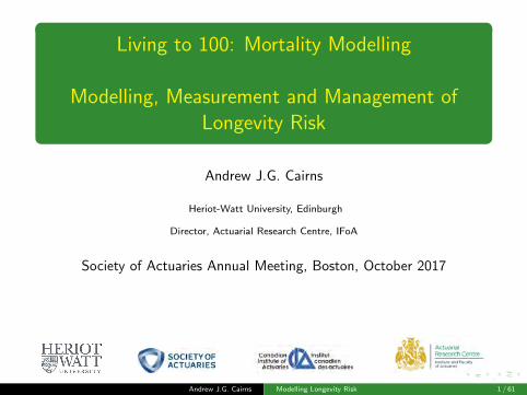
Living to 100: Mortality Modelling
Modelling, Measurement and Management ofLongevity Risk
Andrew J.G. Cairns
Heriot-Watt University, Edinburgh
Director, Actuarial Research Centre, IFoA
Society of Actuaries Annual Meeting, Boston, October 2017
Andrew J.G. Cairns Modelling Longevity Risk 1 / 61

,
The Actuarial Research Centre (ARC)A gateway to global actuarial research
The Actuarial Research Centre (ARC) is the Institute and Faculty ofActuaries’ (IFoA) network of actuarial researchers around the world.The ARC seeks to deliver cutting-edge research programmes that addresssome of the significant, global challenges in actuarial science, through apartnership of the actuarial profession, the academic community andpractitioners.The ’Modelling, Measurement and Management of Longevity andMorbidity Risk’ research programme is being funded by the ARC, theSoA and the CIA.
www.actuaries.org.uk/arc
Andrew J.G. Cairns Modelling Longevity Risk 2 / 61

,
ARC research program themes
Improved models for mortality
Key drivers of mortality
Management of longevity risk
Morbidity risk modelling for critical illnessinsurance
Andrew J.G. Cairns Modelling Longevity Risk 3 / 61

,
Outline
Part 1: All cause mortality modelling
Introduction to stochastic mortality modelsWhy?Example applications
Part 2: Key drivers
Education levelCause of deathHealth inequalities
Andrew J.G. Cairns Modelling Longevity Risk 4 / 61

,
Part 1: All Cause Mortality Modelling
Andrew J.G. Cairns Modelling Longevity Risk 5 / 61

,
US Historical Death Rates
1940 1960 1980 2000 2020 2040
0.00
100.
0025
?
Year
Dea
th R
ate
(log
scal
e)
US Males Aged 20
1940 1960 1980 2000 2020 2040
0.00
20.
004
0.00
8
?
Year
Dea
th R
ate
(log
scal
e)
US Males Aged 40
1940 1960 1980 2000 2020 2040
0.01
00.
020
0.04
0
?
Year
Dea
th R
ate
(log
scal
e)
US Males Aged 60
1940 1960 1980 2000 2020 2040
0.05
0.10
0.20
?
Year
Dea
th R
ate
(log
scal
e)
US Males Aged 80
Andrew J.G. Cairns Modelling Longevity Risk 6 / 61

,
Graphical Diagnostics
Mortality is falling
Different improvement rates at different ages
Different improvement rates over differentperiodsImprovements are random
Short term fluctuationsLong term trends
All stylised factsOther countries:
Some similaritiesSome different patterns
Andrew J.G. Cairns Modelling Longevity Risk 7 / 61

,
Why do we need stochastic mortality models?
Data ⇒ future mortality is uncertain
Good risk management
Setting risk reserves
Regulatory capital requirements (e.g. SolvencyII)
Life insurance contracts with embedded options
Pricing and hedging mortality-linked securities
Andrew J.G. Cairns Modelling Longevity Risk 8 / 61

,
Modelling
Aims:to develop the best models for forecasting futureuncertain mortality;
general desirable criteriacomplexity of model ↔ complexity ofproblem;longevity versus brevity risk;
measurement of risk;
valuation of future risky cashflows.
Andrew J.G. Cairns Modelling Longevity Risk 9 / 61

,
Management
Aims:active management of mortality and longevityrisk;
internal (e.g. product design; naturalhedging)over-the-counter deals (OTC)securitisation
part of overall package of good riskmanagement.
Andrew J.G. Cairns Modelling Longevity Risk 10 / 61
,
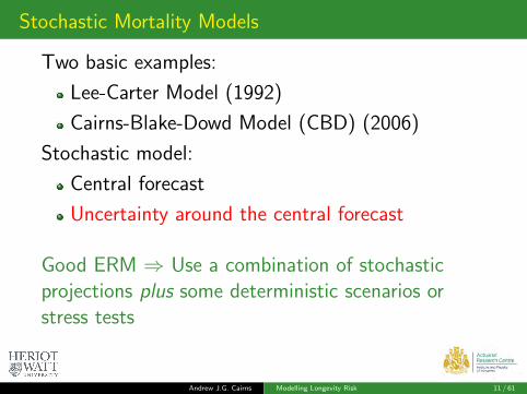
Stochastic Mortality Models
Two basic examples:
Lee-Carter Model (1992)
Cairns-Blake-Dowd Model (CBD) (2006)
Stochastic model:
Central forecast
Uncertainty around the central forecast
Good ERM ⇒ Use a combination of stochasticprojections plus some deterministic scenarios orstress tests
Andrew J.G. Cairns Modelling Longevity Risk 11 / 61

,
The Lee-Carter Model
Death rate:
m(t, x) =D(t, x)
E (t, x)=
deaths(t, x)
average population(t, x)
Year t; Age x .
LC: logm(t, x) = α(x) + β(x)κ(t)
α(x) = base table; age effect
β(x) = age effect
κ(t) = period effect
Andrew J.G. Cairns Modelling Longevity Risk 12 / 61

,
The Lee-Carter Model
logm(t, x) = α(x) + β(x)κ(t)
Estimate α(x), β(x), κ(t) from historical data“Traditional” model:
Fit a random walk model to historical κ(t)Simulate future scenarios for κ(t)Calculate future mortality scenarios givenκ(t)
Alternative models for κ(t) can be used
Andrew J.G. Cairns Modelling Longevity Risk 13 / 61

,
The CBD Model
q(t, x) = Probability of death in year t giveninitially exact age x .
q(t, x) ≈ 1− exp[−m(t, x)]
logit q(t, x) = log
(q
1− q
)= κ1(t) + κ2(t)(x − x̄)
κ1(t) = period effect; affects level
κ2(t) = period effect; affects slope
x̄ = mean age
Captures big picture at higher ages
Andrew J.G. Cairns Modelling Longevity Risk 14 / 61

,
Comparison
LC ⇒ all mortality rates dependent on a single κ(t)⇒ rates at all ages perfectly correlated
CBD ⇒ simpler age effects (1 and x − x̄)but two period effects⇒ richer correlation structure
CBD linearity ⇒not good for younger ages
Historical data:Different improvements at different ages over differenttime periods⇒ need more than one period effect
Andrew J.G. Cairns Modelling Longevity Risk 15 / 61

,
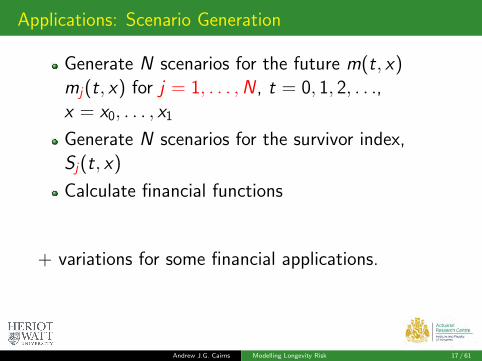
Applications: Scenario Generation
Example: the Lee Carter Model
(Applied to a synthetic dataset)
logm(t, x) = α(x) + β(x)κ(t)
Choose a time series model for κ(t)
Calibrate the time series parameters using dataup to the current time (time 0)
Generate j = 1, . . . ,N stochastic scenarios ofκ(t)
κ1(t), . . . , κN(t)
Andrew J.G. Cairns Modelling Longevity Risk 16 / 61
,
Applications: Scenario Generation
Generate N scenarios for the future m(t, x)mj(t, x) for j = 1, . . . ,N , t = 0, 1, 2, . . .,x = x0, . . . , x1
Generate N scenarios for the survivor index,Sj(t, x)
Calculate financial functions
+ variations for some financial applications.
Andrew J.G. Cairns Modelling Longevity Risk 17 / 61

,
Applications: Scenario Generation, κ(t)
−30 −20 −10 0 10 20 30
−1.
0−
0.5
0.0
0.5
Historical Simulated
Period Effect: One Scenario
Time
Per
iod
Effe
ct, k
appa
(t)
κ(t): Generate scenario 1
Andrew J.G. Cairns Modelling Longevity Risk 18 / 61
,
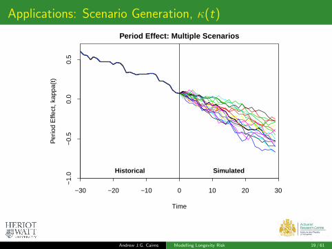
Applications: Scenario Generation, κ(t)
−30 −20 −10 0 10 20 30
−1.
0−
0.5
0.0
0.5
Historical Simulated
Period Effect: Multiple Scenarios
Time
Per
iod
Effe
ct, k
appa
(t)
Andrew J.G. Cairns Modelling Longevity Risk 19 / 61

,
Applications: Scenario Generation, κ(t)
−30 −20 −10 0 10 20 30
−1.
0−
0.5
0.0
0.5
Historical Simulated
Period Effect: Fan Chart
Time
Per
iod
Effe
ct, k
appa
(t)
Andrew J.G. Cairns Modelling Longevity Risk 20 / 61

,
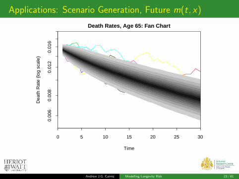
Applications: Scenario Generation, Future m(t, x)
0 5 10 15 20 25 30
0.00
60.
008
0.01
20.
016
Death Rates, Age 65: One Scenario
Time
Dea
th R
ate
(log
scal
e)
Andrew J.G. Cairns Modelling Longevity Risk 21 / 61

,
Applications: Scenario Generation, Future m(t, x)
0 5 10 15 20 25 30
0.00
60.
008
0.01
20.
016
Death Rates, Age 65: Multiple Scenarios
Time
Dea
th R
ate
(log
scal
e)
Andrew J.G. Cairns Modelling Longevity Risk 22 / 61
,
Applications: Scenario Generation, Future m(t, x)
0 5 10 15 20 25 30
0.00
60.
008
0.01
20.
016
Death Rates, Age 65: Fan Chart
Time
Dea
th R
ate
(log
scal
e)
Andrew J.G. Cairns Modelling Longevity Risk 23 / 61
,
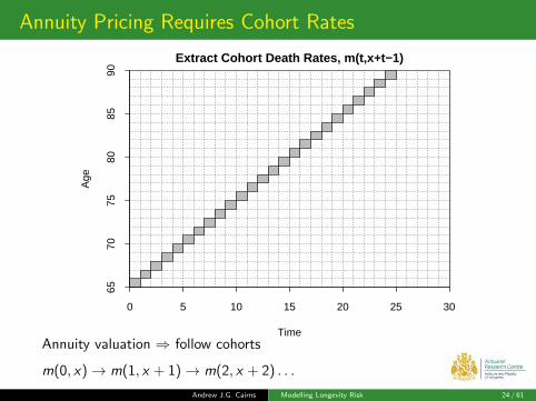
Annuity Pricing Requires Cohort Rates
0 5 10 15 20 25 30
6570
7580
8590
Extract Cohort Death Rates, m(t,x+t−1)
Time
Age
Annuity valuation ⇒ follow cohorts
m(0, x)→ m(1, x + 1)→ m(2, x + 2) . . .
Andrew J.G. Cairns Modelling Longevity Risk 24 / 61

,
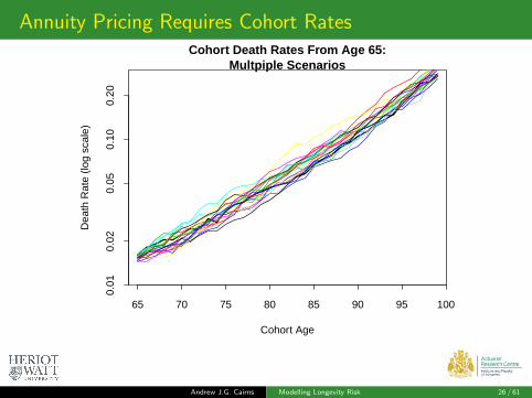
Annuity Pricing Requires Cohort Rates
65 70 75 80 85 90 95 100
0.01
0.02
0.05
0.10
0.20
Cohort Death Rates From Age 65:One Scenario
Cohort Age
Dea
th R
ate
(log
scal
e)
Annuity valuation ⇒ follow cohorts
m(0, x)→ m(1, x + 1)→ m(2, x + 2) . . .
Andrew J.G. Cairns Modelling Longevity Risk 25 / 61
,
Annuity Pricing Requires Cohort Rates
65 70 75 80 85 90 95 100
0.01
0.02
0.05
0.10
0.20
Cohort Death Rates From Age 65:Multpiple Scenarios
Cohort Age
Dea
th R
ate
(log
scal
e)
Andrew J.G. Cairns Modelling Longevity Risk 26 / 61
,
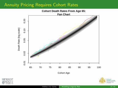
Annuity Pricing Requires Cohort Rates
65 70 75 80 85 90 95 100
0.01
0.02
0.05
0.10
0.20
Cohort Death Rates From Age 65:Fan Chart
Cohort Age
Dea
th R
ate
(log
scal
e)
Andrew J.G. Cairns Modelling Longevity Risk 27 / 61

,
Cohort Survivor Index
65 70 75 80 85 90 95 100
0.0
0.2
0.4
0.6
0.8
1.0
Survivorship From Age 65:One Scenario
Cohort Age
Sur
vivo
r In
dex
(log
scal
e)
Cohort death rates −→ cohort survivorship
Andrew J.G. Cairns Modelling Longevity Risk 28 / 61

,
Cohort Survivor Index
65 70 75 80 85 90 95 100
0.0
0.2
0.4
0.6
0.8
1.0
Survivorship From Age 65:Multiple Scenarios
Cohort Age
Sur
vivo
r In
dex
(log
scal
e)
Andrew J.G. Cairns Modelling Longevity Risk 29 / 61

,
Cohort Survivor Index
65 70 75 80 85 90 95 100
0.0
0.2
0.4
0.6
0.8
1.0
Survivorship From Age 65:Fan Chart
Cohort Age
Sur
vivo
r In
dex
(log
scal
e)
Andrew J.G. Cairns Modelling Longevity Risk 30 / 61

,
Life Expectancy
17 18 19 20 21 22
010
020
030
040
050
0
Cohort Life Expectancy from Age 65
Life Expectancy From Age 65
Fre
quen
cy
17 18 19 20 21 22
0.0
0.2
0.4
0.6
0.8
1.0
Cohort Life Expectancy from Age 65
Life Expectancy From Age 65
Cum
ulat
ive
Pro
babi
lity
Cohort survivorship −→ ex post cohort life expectancyEquivalent to a continuous annuity with 0% interest
Andrew J.G. Cairns Modelling Longevity Risk 31 / 61

,
Annuity Reserving
14 15 16 17
020
040
060
080
0
Present Value of Annuity from Age 65
Present Value ofAnnuity From Age 65
Fre
quen
cy
13.5 14.5 15.5 16.5
0.0
0.2
0.4
0.6
0.8
1.0
Present Value of Annuity from Age 65
Present Value ofAnnuity From Age 65
Cum
ulat
ive
Pro
babi
lity
Annuity of 1 per annum payable annually in arrears
Interest rate: 2%
Andrew J.G. Cairns Modelling Longevity Risk 32 / 61

,
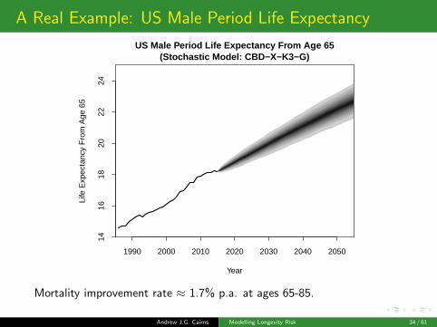
A Real Example: US Male Period Life Expectancy
0 5 10 15 20 25 30
6570
7580
8590
Extract Period Death Rates, m(t,x+t−1)
Time
Age
Andrew J.G. Cairns Modelling Longevity Risk 33 / 61
,
A Real Example: US Male Period Life Expectancy
1990 2000 2010 2020 2030 2040 2050
1416
1820
2224
Year
Life
Exp
ecta
ncy
Fro
m A
ge 6
5
US Male Period Life Expectancy From Age 65(Stochastic Model: CBD−X−K3−G)
Mortality improvement rate ≈ 1.7% p.a. at ages 65-85.
Andrew J.G. Cairns Modelling Longevity Risk 34 / 61

,
How to incorporate Expert Judgement?
E.g. CBD model ⇒mj
CBD(t, x) scenariosm̄CBD(t, x) central forecast
Expert judgement ⇒m̂(t, x) (central) forecast
Blending ⇒ stochastic scenario j becomes
mj(t, x) =mj
CBD(t, x)
m̄CBD(t, x)× m̂(t, x)
Fully stochastic ⇒ full risk assessment
Andrew J.G. Cairns Modelling Longevity Risk 35 / 61
,
How to incorporate Expert Judgement?
A variation on this is required by UK lifeinsurance regulators
⇒ Don’t ignore stochastic models simplybecause you disagree with the central forecast!
Additionally: new approaches to bring the twotogether are being developed
Andrew J.G. Cairns Modelling Longevity Risk 36 / 61

,
Part 2: Key Drivers
Andrew J.G. Cairns Modelling Longevity Risk 37 / 61

,
Drill into the Detail of US Data
Level of educational attainment ⇒ predictor
Individual cause of death ⇒ outcome
Beware of grade inflation
Help to understand trends in national data andsubpopulations (e.g. white collar pension plan)
Andrew J.G. Cairns Modelling Longevity Risk 38 / 61
,
Data Sources
Total Exposures: Human Mortality Database(smoothed to mitigate anomalies)
CDC deaths: cause of death + education(+ ethnic group)
CPS survey data: education proportions
Research ⇒smart synthesis of three data sources
improved, less noisy, exposures by education level
Andrew J.G. Cairns Modelling Longevity Risk 39 / 61
,
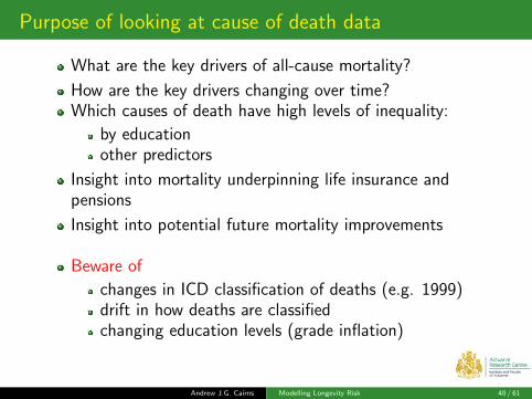
Purpose of looking at cause of death data
What are the key drivers of all-cause mortality?
How are the key drivers changing over time?Which causes of death have high levels of inequality:
by educationother predictors
Insight into mortality underpinning life insurance andpensions
Insight into potential future mortality improvements
Beware of
changes in ICD classification of deaths (e.g. 1999)drift in how deaths are classifiedchanging education levels (grade inflation)
Andrew J.G. Cairns Modelling Longevity Risk 40 / 61

,
Education Levels
EducationLow education Primary and lower secondary educationMedium education Upper secondary educationHigh education Tertiary education
Andrew J.G. Cairns Modelling Longevity Risk 41 / 61

,
Cause of Death Groupings
1 Infectious diseases incl. tuberculosis 2 Cancer: mouth, gullet, stomach3 Cancer: gut, rectum 4 Cancer: lung, larynx, ..5 Cancer: breast 6 Cancer: uterus, cervix7 Cancer: prostate, testicular 8 Cancer: bones, skin9 Cancer: lymphatic, blood-forming tissue 10 Benign tumours11 Diseases: blood 12 Diabetes13 Mental illness 14 Meningitis + nervous system (Alzh.)15 Blood pressure + rheumatic fever 16 Ischaemic heart diseases17 Other heart diseases 18 Diseases: cerebrovascular19 Diseases: circulatory 20 Diseases: lungs, breathing21 Diseases: digestive 22 Diseases: urine, kidney,...23 Diseases: skin, bone, tissue 24 Senility without mental illness25 Road/other accidents 26 Other causes27 Alcohol → liver disease 28 Suicide29 Accidental Poisonings
Andrew J.G. Cairns Modelling Longevity Risk 42 / 61

,
US Education Data
Males and Females (2)
Single ages 55-75 (21)
Single years 1989-2015 (27)
Causes of death (29)
Low, medium & high education level (3)
Note: HMD’s Human Cause of Death Database ⇒All ages (5’s), 1999-2015, No education
Andrew J.G. Cairns Modelling Longevity Risk 43 / 61

,
US Education Data: Growing Inequality, Males
55 60 65 70 75
0.00
20.
005
0.01
00.
020
0.05
00.
100
1989
2015
1989
2015
High
Low
Low Ed 1989Low Ed 2002Low Ed 2015High Ed 1989High Ed 2002High Ed 2015
Age
Dea
th R
ate
(log
scal
e)Male All Cause Death Rates by Education Group
For 1989 and 2015
Andrew J.G. Cairns Modelling Longevity Risk 44 / 61
,
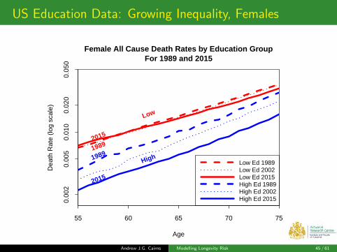
US Education Data: Growing Inequality, Females
55 60 65 70 75
0.00
20.
005
0.01
00.
020
0.05
0
19892015
1989
2015
High
Low
Low Ed 1989Low Ed 2002Low Ed 2015High Ed 1989High Ed 2002High Ed 2015
Age
Dea
th R
ate
(log
scal
e)Female All Cause Death Rates by Education Group
For 1989 and 2015
Andrew J.G. Cairns Modelling Longevity Risk 45 / 61
,
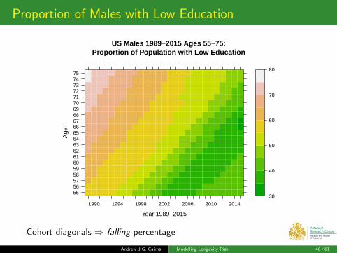
Proportion of Males with Low Education
US Males 1989−2015 Ages 55−75:Proportion of Population with Low Education
Year 1989−2015
Age
555657585960616263646566676869707172737475
1990 1994 1998 2002 2006 2010 2014
30
40
50
60
70
80
Cohort diagonals ⇒ falling percentage
Andrew J.G. Cairns Modelling Longevity Risk 46 / 61

,
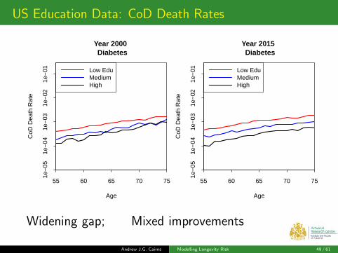
US Education Data: CoD Death Rates
55 60 65 70 75
1e−
051e
−04
1e−
031e
−02
1e−
01 Low EduMediumHigh
Year 2000 Ischaemic heart diseases
Age
CoD
Dea
th R
ate
55 60 65 70 75
1e−
051e
−04
1e−
031e
−02
1e−
01 Low EduMediumHigh
Year 2015 Ischaemic heart diseases
Age
CoD
Dea
th R
ate
Widening gap
Andrew J.G. Cairns Modelling Longevity Risk 47 / 61

,
US Education Data: CoD Death Rates
55 60 65 70 75
1e−
051e
−04
1e−
031e
−02
1e−
01 Low EduMediumHigh
Year 2000 Cancer: lung, larynx, ..
Age
CoD
Dea
th R
ate
55 60 65 70 75
1e−
051e
−04
1e−
031e
−02
1e−
01 Low EduMediumHigh
Year 2015 Cancer: lung, larynx, ..
Age
CoD
Dea
th R
ate
Widening gap
Andrew J.G. Cairns Modelling Longevity Risk 48 / 61
,
US Education Data: CoD Death Rates
55 60 65 70 75
1e−
051e
−04
1e−
031e
−02
1e−
01 Low EduMediumHigh
Year 2000 Diabetes
Age
CoD
Dea
th R
ate
55 60 65 70 75
1e−
051e
−04
1e−
031e
−02
1e−
01 Low EduMediumHigh
Year 2015 Diabetes
Age
CoD
Dea
th R
ate
Widening gap; Mixed improvements
Andrew J.G. Cairns Modelling Longevity Risk 49 / 61
,
US Education Data: CoD Death Rates
55 60 65 70 75
1e−
051e
−04
1e−
031e
−02
1e−
01 Low EduMediumHigh
Year 2000 Meningitis + nervous system (Alzh.)
Age
CoD
Dea
th R
ate
55 60 65 70 75
1e−
051e
−04
1e−
031e
−02
1e−
01 Low EduMediumHigh
Year 2015 Meningitis + nervous system (Alzh.)
Age
CoD
Dea
th R
ate
Widening gap; almost no improvements
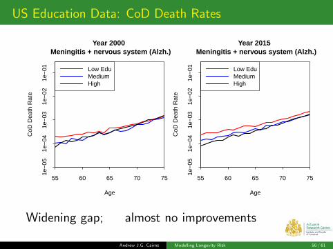
Andrew J.G. Cairns Modelling Longevity Risk 50 / 61

,
US Education Data: CoD Death Rates
55 60 65 70 75
1e−
051e
−04
1e−
031e
−02
1e−
01 Low EduMediumHigh
Year 2000 Accidental Poisonings
Age
CoD
Dea
th R
ate
55 60 65 70 75
1e−
051e
−04
1e−
031e
−02
1e−
01 Low EduMediumHigh
Year 2015 Accidental Poisonings
Age
CoD
Dea
th R
ate
Case & Deaton (2015) ⇒ Accidental poisoning ↗
Andrew J.G. Cairns Modelling Longevity Risk 51 / 61
,
US Education Data: CoD Death Rates
55 60 65 70 75
1e−
051e
−04
1e−
031e
−02
1e−
01 Low EduMediumHigh
Year 2000 Alcohol −> liver
Age
CoD
Dea
th R
ate
55 60 65 70 75
1e−
051e
−04
1e−
031e
−02
1e−
01 Low EduMediumHigh
Year 2015 Alcohol −> liver
Age
CoD
Dea
th R
ate
Widening gap
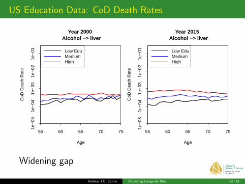
Andrew J.G. Cairns Modelling Longevity Risk 52 / 61
,
US Education Data: CoD Death Rates
55 60 65 70 75
1e−
051e
−04
1e−
031e
−02
1e−
01 Low EduMediumHigh
Year 2000 Cancer: prostate, testicular
Age
CoD
Dea
th R
ate
55 60 65 70 75
1e−
051e
−04
1e−
031e
−02
1e−
01 Low EduMediumHigh
Year 2015 Cancer: prostate, testicular
Age
CoD
Dea
th R
ate
Denmark ⇒ almost NO gap by education;Denmark ⇒ small gap by affluence; smaller than US by education
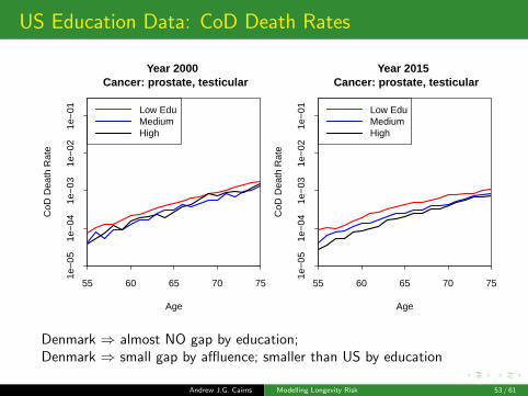
Andrew J.G. Cairns Modelling Longevity Risk 53 / 61
,
Cause of Death Data: Health Inequalities
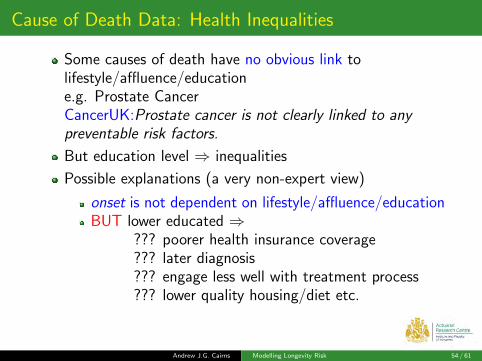
Some causes of death have no obvious link tolifestyle/affluence/educatione.g. Prostate CancerCancerUK:Prostate cancer is not clearly linked to anypreventable risk factors.
But education level ⇒ inequalities
Possible explanations (a very non-expert view)
onset is not dependent on lifestyle/affluence/educationBUT lower educated ⇒
??? poorer health insurance coverage??? later diagnosis??? engage less well with treatment process??? lower quality housing/diet etc.
Andrew J.G. Cairns Modelling Longevity Risk 54 / 61

,
US Males: Low versus High Education
Do Low and High education groups have the sameCoD rate?
Four × 5-year age groups
29 causes of death
Signs Test (count low edu. > high edu. mort.)
29× 4 = 116 individual tests
Reject equality hypothesis in all but one test
Accept H0 (p = 0.08) for only one pairing:Meningitis + nervous system (Alzh.), 70-74
Most p-values < 10−6
Andrew J.G. Cairns Modelling Longevity Risk 55 / 61

,
Summary
Future work
Analysis of sub-national datasetse.g. SoA Group and Individual Annuity datae.g. individual pension plan dataMultiple population modelling
E: [email protected] W: www.macs.hw.ac.uk/∼andrewc
Andrew J.G. Cairns Modelling Longevity Risk 56 / 61

,
Thank You!
Questions?
E: [email protected] W: www.macs.hw.ac.uk/∼andrewc
Andrew J.G. Cairns Modelling Longevity Risk 57 / 61
,
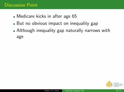
Discussion Point
Medicare kicks in after age 65
But no obvious impact on inequality gap
Although inequality gap naturally narrows withage
Andrew J.G. Cairns Modelling Longevity Risk 58 / 61

,
CoD Death Rates: Different Shapes & Patterns
40 50 60 70 80 90
1e−
051e
−04
1e−
031e
−02
1e−
01Infectious diseases incl. tuberculosis
Dea
th R
ate
(log
scal
e)
12345678910
40 50 60 70 80 90
1e−
051e
−04
1e−
031e
−02
1e−
01
Meningitis + nervous system (Alzh.)
Dea
th R
ate
(log
scal
e)
12345678910
40 50 60 70 80 90
1e−
051e
−04
1e−
031e
−02
1e−
01
Ischaemic heart diseases
Dea
th R
ate
(log
scal
e)
12345678910
40 50 60 70 80 90
1e−
051e
−04
1e−
031e
−02
1e−
01
Diseases: circulatory
Dea
th R
ate
(log
scal
e)
12345678910
40 50 60 70 80 90
1e−
051e
−04
1e−
031e
−02
1e−
01Diseases: lungs, breathing
Dea
th R
ate
(log
scal
e)
12345678910
40 50 60 70 80 90
1e−
051e
−04
1e−
031e
−02
1e−
01
Diseases: urine, kidney,...
Dea
th R
ate
(log
scal
e)
12345678910
Andrew J.G. Cairns Modelling Longevity Risk 59 / 61

,
CoD Death Rates: Different Shapes & Patterns
40 50 60 70 80 90
1e−
051e
−03
1e−
01
Cancer: gut, rectum
Dea
th R
ate
(log
scal
e)
12345678910
40 50 60 70 80 90
1e−
051e
−03
1e−
01
Cancer: lung, larynx, ..
Dea
th R
ate
(log
scal
e)
12345678910
40 50 60 70 80 90
1e−
051e
−03
1e−
01
Cancer: prostate, testicular
Dea
th R
ate
(log
scal
e)
12345678910
40 50 60 70 80 90
1e−
051e
−03
1e−
01
Cancer: bones, skin
Dea
th R
ate
(log
scal
e)
12345678910
Andrew J.G. Cairns Modelling Longevity Risk 60 / 61
,
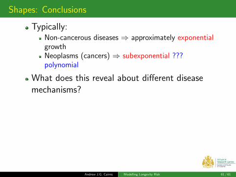
Shapes: Conclusions
Typically:Non-cancerous diseases ⇒ approximately exponentialgrowthNeoplasms (cancers) ⇒ subexponential ???polynomial
What does this reveal about different diseasemechanisms?
Andrew J.G. Cairns Modelling Longevity Risk 61 / 61

Declining Mortality (Increasing Longevity):At What Rate?
Steve Goss, Chief ActuarySocial Security Administration
Session 122Society of Actuaries Annual Meeting
October 17, 2017
2
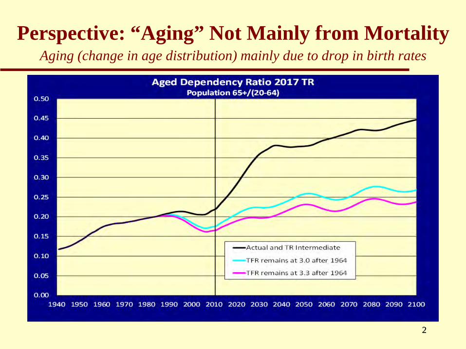
Perspective: “Aging” Not Mainly from MortalityAging (change in age distribution) mainly due to drop in birth rates
2
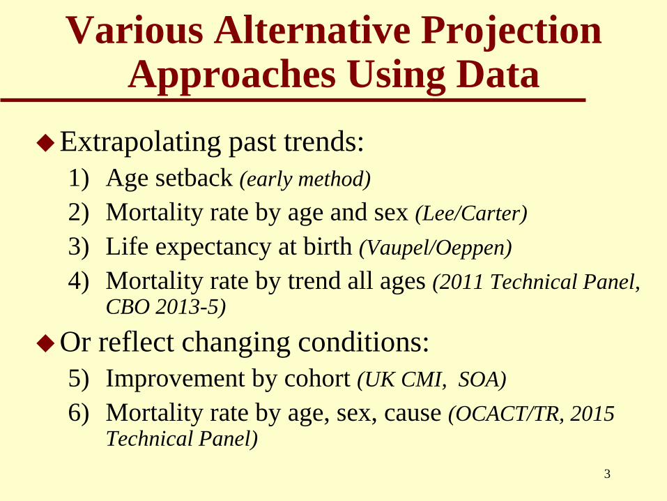
Various Alternative Projection Approaches Using Data
Extrapolating past trends:1) Age setback (early method)2) Mortality rate by age and sex (Lee/Carter)3) Life expectancy at birth (Vaupel/Oeppen)4) Mortality rate by trend all ages (2011 Technical Panel,
CBO 2013-5)
Or reflect changing conditions:5) Improvement by cohort (UK CMI, SOA)6) Mortality rate by age, sex, cause (OCACT/TR, 2015
Technical Panel)3
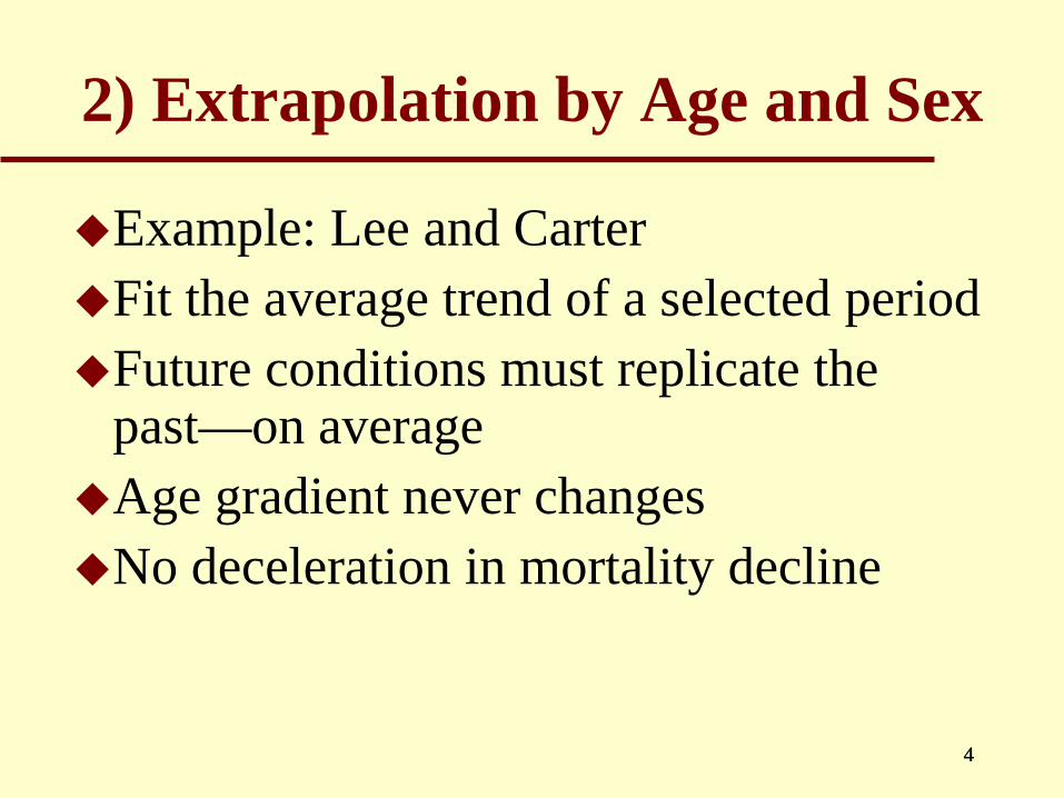
2) Extrapolation by Age and Sex
Example: Lee and CarterFit the average trend of a selected periodFuture conditions must replicate the
past—on averageAge gradient never changesNo deceleration in mortality decline
44
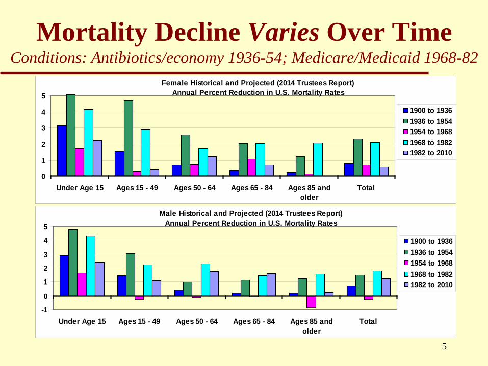
Mortality Decline Varies Over TimeConditions: Antibiotics/economy 1936-54; Medicare/Medicaid 1968-82
Female Historical and Projected (2014 Trustees Report) Annual Percent Reduction in U.S. Mortality Rates
0
1
2
3
4
5
Under Age 15 Ages 15 - 49 Ages 50 - 64 Ages 65 - 84 Ages 85 andolder
Total
1900 to 19361936 to 19541954 to 19681968 to 19821982 to 2010
Male Historical and Projected (2014 Trustees Report) Annual Percent Reduction in U.S. Mortality Rates
-10
123
45
Under Age 15 Ages 15 - 49 Ages 50 - 64 Ages 65 - 84 Ages 85 andolder
Total
1900 to 19361936 to 19541954 to 19681968 to 19821982 to 2010
5

3) Will Life Expectancy Rise Linearly?Vaupel/Oeppen 2002; Best Nations
Requires acceleratingrate of decline in mortality rates if retain age gradient
LE most affected by lowest ages—only so much gain possible
Most disagree– Vallin/Meslé
6

4) Extrapolate All Ages the Same
Ignores historical age gradientResult:
– Substantial bias for population age distributionThus, large bias for cost as % of payroll
– Less mortality decline at young ages raises cost– More mortality decline at higher ages raises cost
7
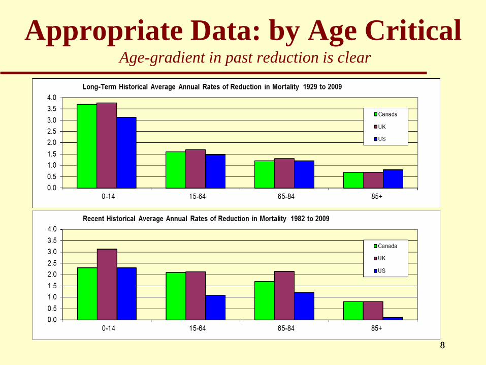
Appropriate Data: by Age CriticalAge-gradient in past reduction is clear
88

5) Extrapolation by Cohort
U.K. (& SOA-RPEC): “Phantoms never die” data issues
Post-WW2 births: antibiotics young, statins later What does change up to age x say above age x? Is cohort healthier at x if lower mortality up to x?Or is cohort compromised by impaired survivors?What does one cohort imply for the next cohort?
Period effects from known changes in conditions are stronger—especially in the U.S.
99
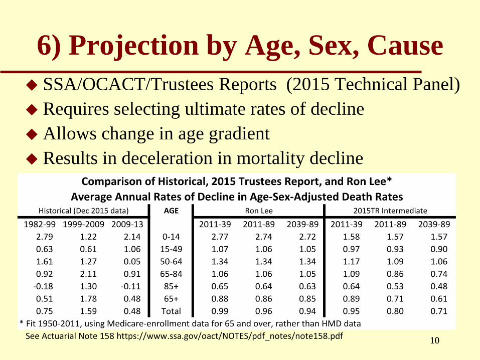
6) Projection by Age, Sex, Cause SSA/OCACT/Trustees Reports (2015 Technical Panel) Requires selecting ultimate rates of decline Allows change in age gradient Results in deceleration in mortality decline
AGE
1982-99 1999-2009 2009-13 2011-39 2011-89 2039-89 2011-39 2011-89 2039-892.79 1.22 2.14 0-14 2.77 2.74 2.72 1.58 1.57 1.570.63 0.61 1.06 15-49 1.07 1.06 1.05 0.97 0.93 0.901.61 1.27 0.05 50-64 1.34 1.34 1.34 1.17 1.09 1.060.92 2.11 0.91 65-84 1.06 1.06 1.05 1.09 0.86 0.74
-0.18 1.30 -0.11 85+ 0.65 0.64 0.63 0.64 0.53 0.480.51 1.78 0.48 65+ 0.88 0.86 0.85 0.89 0.71 0.610.75 1.59 0.48 Total 0.99 0.96 0.94 0.95 0.80 0.71
* Fit 1950-2011, using Medicare-enrollment data for 65 and over, rather than HMD data See Actuarial Note 158 https://www.ssa.gov/oact/NOTES/pdf_notes/note158.pdf
2015TR Intermediate
Comparison of Historical, 2015 Trustees Report, and Ron Lee* Average Annual Rates of Decline in Age-Sex-Adjusted Death Rates
Historical (Dec 2015 data) Ron Lee
1010

Age-adjusted Death Rates for Heart Disease, Cancer, Stroke, and Unintentional Injuries: United States, 1900-2015
(courtesy Robert Anderson, NCHS)Rate per 100,000 standard population
NOTE: Data prior to 1933 contain death-registration States only. Data for 2015 is provisional.
Heart disease
Cancer
StrokeUnintentional injuries
11

Mortality Decline by Cause of Death: Rate of change from 1979 to 2013
-4
-3
-2
-1
0
1
2
3
4
Under 15 15-49 50-64 65-84 85+
CardiovascularCancerViolenceRespiratoryOther
FEMALE
-3
-2
-1
0
1
2
3
4
Under 15 15-49 50-64 65-84 85+
MALE
12

Age-Sex Extrapolation vs. Age-Sex-Cause Projection Lee maintaining full age-gradient offsets lack of deceleration
Result: OASDI actuarial deficit unchanged using Lee estimates
Mortality Rate Comparison Age 0-14 Unisex
0
1
2
3
4
5
6
1950 1970 1990 2010 2030 2050 2070 2090
Historical 2015TR Ron Lee
Mortality Rate Comparison Age 65+ Unisex
7.5
8
8.5
9
1950 1970 1990 2010 2030 2050 2070 2090
Historical 2015TR Ron Lee
1313
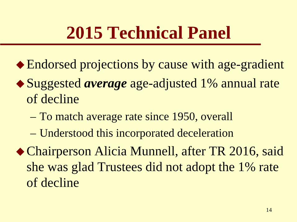
2015 Technical PanelEndorsed projections by cause with age-gradientSuggested average age-adjusted 1% annual rate
of decline– To match average rate since 1950, overall– Understood this incorporated deceleration
Chairperson Alicia Munnell, after TR 2016, said she was glad Trustees did not adopt the 1% rate of decline
14

Mortality Experience: All AgesReductions continue to fall short of expectations
151515

Mortality Experience: Ages 65 and OlderReductions since 2009 continue to fall short of expectations
161616
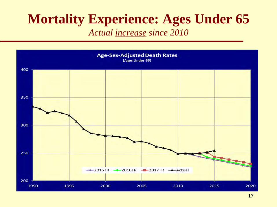
Mortality Experience: Ages Under 65 Actual increase since 2010
171717
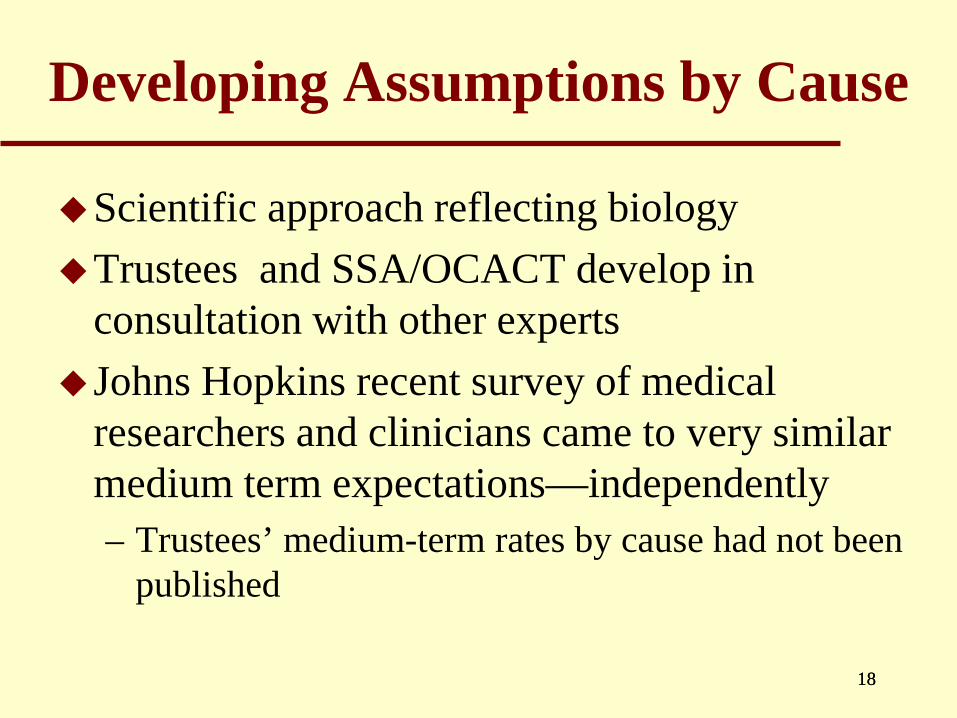
Developing Assumptions by Cause
Scientific approach reflecting biologyTrustees and SSA/OCACT develop in
consultation with other expertsJohns Hopkins recent survey of medical
researchers and clinicians came to very similar medium term expectations—independently– Trustees’ medium-term rates by cause had not been
published
1818

Cardiovascular: JHU Less Optimistic than Trustees over Age 50 for Next 30 Years
19
0.0
0.5
1.0
1.5
2.0
2.5
3.0
3.5
4.0
Under Age 15 Ages 15 - 49 Ages 50 - 64 Ages 65 - 84 Ages 85 andolder
Total
Cardiovascular Disease-FemaleAverage Annual Percent Reduction
JHU values are for the period 2009-2040
1979 to 2010
2010 to 2038
2038 to 2088
JHU 0.5
JHU 1.5JHU
1.6
JHU 1.5
0.0
0.5
1.0
1.5
2.0
2.5
3.0
3.5
4.0
Under Age 15 Ages 15 - 49 Ages 50 - 64 Ages 65 - 84 Ages 85 andolder
Total
Cardiovascular Disease-MaleAverage Annual Percent Reduction
JHU values are for the period 2009-2040
1979 to 2010
2010 to 2038
2038 to 2088
JHU 1.1 JHU
0.6
JHU 1.5JHU
1.6
1919
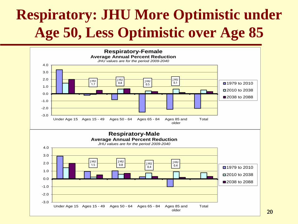
Respiratory: JHU More Optimistic under Age 50, Less Optimistic over Age 85
20
-3.0
-2.0
-1.0
0.0
1.0
2.0
3.0
4.0
Under Age 15 Ages 15 - 49 Ages 50 - 64 Ages 65 - 84 Ages 85 andolder
Total
Respiratory-FemaleAverage Annual Percent Reduction
JHU values are for the period 2009-2040
1979 to 2010
2010 to 2038
2038 to 2088
JHU 0.1JHU
0.5JHU 0.8
JHU 1.7
-3.0
-2.0
-1.0
0.0
1.0
2.0
3.0
4.0
Under Age 15 Ages 15 - 49 Ages 50 - 64 Ages 65 - 84 Ages 85 andolder
Total
Respiratory-MaleAverage Annual Percent Reduction
JHU values are for the period 2009-2040
1979 to 2010
2010 to 2038
2038 to 2088
JHU 0.4JHU
0.4
JHU 0.8
JHU 1.5
2020
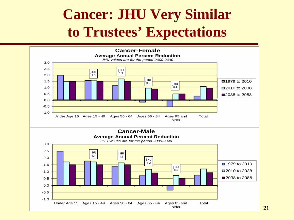
Cancer: JHU Very Similar to Trustees’ Expectations
21
-1.0
-0.5
0.0
0.5
1.0
1.5
2.0
2.5
3.0
Under Age 15 Ages 15 - 49 Ages 50 - 64 Ages 65 - 84 Ages 85 andolder
Total
Cancer-FemaleAverage Annual Percent Reduction
JHU values are for the period 2009-2040
1979 to 2010
2010 to 2038
2038 to 2088
JHU 0.4
JHU 0.9
JHU 1.3JHU
1.8
-1.0
-0.5
0.0
0.5
1.0
1.5
2.0
2.5
3.0
Under Age 15 Ages 15 - 49 Ages 50 - 64 Ages 65 - 84 Ages 85 andolder
Total
Cancer-MaleAverage Annual Percent Reduction
JHU values are for the period 2009-2040
1979 to 2010
2010 to 2038
2038 to 2088
JHU 0.6
JHU 1.2
JHU 1.1
JHU 1.3
2121
How Future Conditions Might Change
Smoking decline for women– Started and stopped later than men
Obesity—sedentary lifestyleDifference by income/earningsHealth spending—must decelerate
– Advances help only if apply to allHuman limits
– Increasing understanding of deceleration2222

Trends in Obesity: US 1971-2006 Sam Preston 2010—must consider cumulative effects
Increasing duration of obesity for aged in future
2323

Death Rates Vary by Career Earnings Ranking Difference has increased
Female 65-69 Retired-Worker Relative Death Rates by AIME Quartile
00.20.40.60.8
11.21.41.6
1 2 3 4
19902010
24
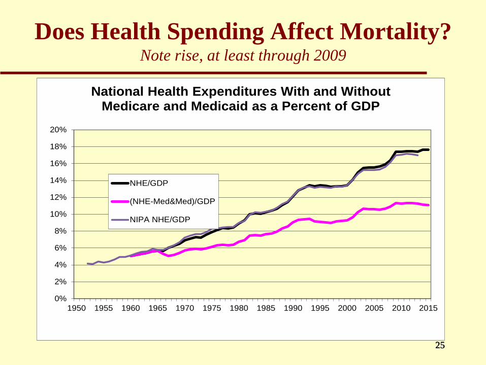
Does Health Spending Affect Mortality?Note rise, at least through 2009
25
0%
2%
4%
6%
8%
10%
12%
14%
16%
18%
20%
1950 1955 1960 1965 1970 1975 1980 1985 1990 1995 2000 2005 2010 2015
National Health Expenditures With and Without Medicare and Medicaid as a Percent of GDP
NHE/GDP
(NHE-Med&Med)/GDP
NIPA NHE/GDP
2525
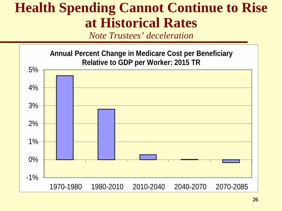
Health Spending Cannot Continue to Rise at Historical RatesNote Trustees’ deceleration
26
-1%
0%
1%
2%
3%
4%
5%
1970-1980 1980-2010 2010-2040 2040-2070 2070-2085
Annual Percent Change in Medicare Cost per Beneficiary Relative to GDP per Worker: 2015 TR
2626

Is There an Omega?It appears we are rectangularizing the survival curve?
Survival Curve U.S. Female: Period Data
00.10.20.30.40.50.60.70.80.9
1
0 10 20 30 40 50 60 70 80 90 100 110
190019251950197520002013
Survival Curve U.S. Male: Period Data
00.10.20.30.40.50.60.70.80.9
1
0 10 20 30 40 50 60 70 80 90 100 110
190019251950197520002013
2727
28
Death Rates Will Continue to Decline: But How Fast and for Whom?
Must understand past and future conditions– Persistent historical “age gradient”– Avoid simple extrapolation of past periods
» Cannot ignore changing conditions “Limits” on longevity due to physiology Latter half of 20th century was extraordinary
» So deceleration seems likely» Cause-specific rates allow basis for assumptions
– Results: in the 1982 TR, we projected LE65 in 2013 to be 19.0; actual was 19.1
28

29
For More Information…http://www.ssa.gov/oact/
Documentation of Trustees Report data & assumptions https://www.ssa.gov/oact/TR/2017/2017_Long-Range_Demographic_Assumptions.pdf
Historical and projected mortality rateshttps://www.ssa.gov/oact/HistEst/DeathHome.html
Annual Trustees Reports https://www.ssa.gov/oact/TR/index.html
29


