
Looking for clusters in your data ...Looking for clusters in your data ...(in theory and in practice)(in theory and in practice)
Michael W. Mahoney
Stanford University
4/7/11( For more info, see:
http:// cs.stanford.edu/people/mmahoney/or Google on “Michael Mahoney”)

Outline (and lessons)
1. Matrices and graphs are basic structures for modeling data, and many algorithms boil down to matrix/graph algorithms.
2. Often, algorithms work when they “shouldn’t,” don’t work when they “should,” and interpretation is tricky but often of interest downstream.
3. Analysts tell stories since they often have no idea of what the data “look like,” but algorithms can be used to “explore” or “probe” the data.
4. Large networks (and large data) are typically very different than small networks (and small data), but people typically implicitly assume they are the same.

Machine learning and data analysis, versus “the database” perspective
Many data sets are better-described by graphs or matrices than as dense flat tables• Obvious to some, but a big challenge given the way that databases are constructed and supercomputers are designed
• Sweet spot between descriptive flexibility and algorithmic tractability
• Very different questions than traditional NLA and graph theory/practice as well as traditional database theory/practice
Often, the first step is to partition/cluster the data• Often, this can be done with natural matrix and graph algorithms
• Those algorithms always return answers whether or not the data cluster well
• Often, there is a “positive-results” bias to find things like clusters

Modeling the data as a matrix
We are given m objects and n features describing the objects.
(Each object has n numeric values describing it.)
Dataset
An m-by-n matrix A, Aij shows the “importance” of feature j for object i.
Every row of A represents an object.
Goal
We seek to understand the structure of the data, e.g., the underlying process generating the data.

Market basket matrices
Common representation for association rule mining in databases.
(Sometimes called a “flat table” if matrix operations are not performed.)
m customer
s
n products
(e.g., milk, bread, wine, etc.)
A ij = quantity of j-th product purchased
by the i-th customer
Data mining tasks
- Find association rules, E.g., customers who buy product x buy product y with probability 89%.
- Such rules are used to make item display decisions, advertising decisions, etc.
Term-document matrices
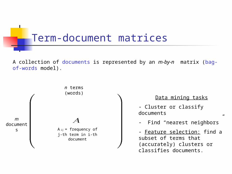
A collection of documents is represented by an m-by-n matrix (bag-of-words model).
m documen
ts
n terms (words)
A ij = frequency of j-th term in i-th document
Data mining tasks
- Cluster or classify documents
- Find “nearest neighbors”
- Feature selection: find a subset of terms that (accurately) clusters or classifies documents.

Recommendation system matrices
The m-by-n matrix A represents m customers and n products.
n products
A ij = utility of j-th product to i-th
customer
Data mining task
• Given a few samples from A, recommend high utility products to customers.
• Recommend queries in advanced match in sponsored search
m customer
s

DNA microarray data matrices
Microarray Data
Rows: genes (ca. 5,500)
Columns: e.g., 46 soft-issue tumor specimens
Tasks:
Pick a subset of genes (if it exists) that suffices in order to identify the “cancer type” of a patient
gene
s
tumour specimens
Nielsen et al., Lancet, 2002

DNA SNP data matrices
Single Nucleotide Polymorphisms: the most common type of genetic variation in the genome across different individuals.
They are known locations at the human genome where two alternate nucleotide bases (alleles) are observed (out of A, C, G, T).
SNPs
indiv
idu
als
… AG CT GT GG CT CC CC CC CC AG AG AG AG AG AA CT AA GG GG CC GG AG CG AC CC AA CC AA GG TT AG CT CG CG CG AT CT CT AG CT AG GG GT GA AG …
… GG TT TT GG TT CC CC CC CC GG AA AG AG AG AA CT AA GG GG CC GG AA GG AA CC AA CC AA GG TT AA TT GG GG GG TT TT CC GG TT GG GG TT GG AA …
… GG TT TT GG TT CC CC CC CC GG AA AG AG AA AG CT AA GG GG CC AG AG CG AC CC AA CC AA GG TT AG CT CG CG CG AT CT CT AG CT AG GG GT GA AG …
… GG TT TT GG TT CC CC CC CC GG AA AG AG AG AA CC GG AA CC CC AG GG CC AC CC AA CG AA GG TT AG CT CG CG CG AT CT CT AG CT AG GT GT GA AG …
… GG TT TT GG TT CC CC CC CC GG AA GG GG GG AA CT AA GG GG CT GG AA CC AC CG AA CC AA GG TT GG CC CG CG CG AT CT CT AG CT AG GG TT GG AA …
… GG TT TT GG TT CC CC CG CC AG AG AG AG AG AA CT AA GG GG CT GG AG CC CC CG AA CC AA GT TT AG CT CG CG CG AT CT CT AG CT AG GG TT GG AA …
… GG TT TT GG TT CC CC CC CC GG AA AG AG AG AA TT AA GG GG CC AG AG CG AA CC AA CG AA GG TT AA TT GG GG GG TT TT CC GG TT GG GT TT GG AA …
Matrices including 100s of individuals and more than 300K SNPs are publicly available.
Task : split the individuals in different clusters depending on their ancestry, and
find a small subset of genetic markers that are “ancestry informative”.

Social networks (e.g., an e-mail network)
Represents, e.g., the email communications between groups of users.
n users
n users
A ij = number of emails exchanged
between users i and j during a certain time
period
Data mining tasks
- cluster the users
- identify “dense” networks of users (dense subgraphs)
- recommend friends
- clusters for bucket testing
- etc.

How people think about networks
“Interaction graph” model of networks: • Nodes represent “entities”• Edges represent “interaction” between pairs of entities
Graphs are combinatorial, not obviously-geometric • Strength: powerful framework for analyzing algorithmic complexity • Drawback: geometry used for learning and statistical inference

Matrices and graphs
Networks are often represented by a graph G=(V,E)• V = vertices/things
• E = edges = interactions between pairs of things
Close connections between matrices and graphs; given a graph, one can study:• Adjacency matrix: Aij = 1 if an edge between nodes i and j
• Combinatorial Laplacian: D-A, where D is diagonal degree matrix
• Normalized Laplacian: I-D-1/2AD-1/2, related to random walks

The Singular Value Decomposition (SVD)
rank of A
U (V): orthogonal matrix containing the left (right) singular vectors of A.
: diagonal matrix containing 1 2 … , the singular values of A.
Often people use this via PCA or MDS or other related methods.
The formal definition:
Given any m x n matrix A, one can decompose it as:

4.0 4.5 5.0 5.5 6.02
3
4
5
1st (right) singular vector
2nd (right) singular vector
Singular values and vectors, intuition
1
2
The SVD of the m-by-2 data matrix (m data points in a 2-D space) returns:• V(i): Captures (successively orthogonalized) directions of variance.• i: Captures how much variance is explained by (each successive) direction.

Rank-k approximations via the SVD
A VTU=
objects
features
significant
noise
nois
e noisesi
gnifi
cant
sig.
=
Very important: Keeping top k singular vectors provides “best” rank-k approximation to A!

Computing the SVD
Many ways; e.g.,• LAPACK - high-quality software library in Fortran for NLA
• MATLAB - call “svd,” “svds,” “eig,” “eigs,” etc.
• R - call “svd” or “eigen”
• NumPy - call “svd” in LinAlgError class
In the past:
• you never computed the full SVD.
• Compute just what you need.
Ques: How true will that be true in the future?

Eigen-methods in ML and data analysis
Eigen-tools appear (explicitly or implicitly) in many data analysis and machine learning tools:
• Latent semantic indexing
• PCA and MDS
• Manifold-based ML methods
• Diffusion-based methods
• k-means clustering
• Spectral partitioning and spectral ranking

Outline (and lessons)
1. Matrices and graphs are basic structures for modeling data, and many algorithms boil down to matrix/graph algorithms.
2. Often, algorithms work when they “shouldn’t,” don’t work when they “should,” and interpretation is tricky but often of interest downstream.
3. Analysts tell stories since they often have no idea of what the data “look like,” but algorithms can be used to “explore” or “probe” the data.
4. Large networks (and large data) are typically very different than small networks (and small data), but people typically implicitly assume they are the same.

HGDP data
• 1,033 samples
• 7 geographic regions
• 52 populations
Cavalli-Sforza (2005) Nat Genet Rev
Rosenberg et al. (2002) Science
Li et al. (2008) Science
The International HapMap Consortium (2003, 2005, 2007), Nature
Matrix dimensions:
2,240 subjects (rows)
447,143 SNPs (columns)The Human Genome Diversity Panel (HGDP)
ASW, MKK, LWK, & YRI
CEU
TSIJPT, CHB, & CHD
GIH
MEX
HapMap Phase 3 data
• 1,207 samples
• 11 populations
HapMap Phase 3
SVD/PCA returns…

Africa
Middle East
South Central Asia
Europe
Oceania
East Asia
America
Gujarati Indians
Mexicans
• Top two Principal Components (PCs or eigenSNPs) (Lin and Altman (2005) Am J Hum Genet)
• The figure renders visual support to the “out-of-Africa” hypothesis.
• Mexican population seems out of place: we move to the top three PCs.
Paschou, Lewis, Javed, & Drineas (2010) J Med Genet

AfricaMiddle East
S C Asia & Gujarati Europe
Oceania
East Asia
America
Not altogether satisfactory: the principal components are linear combinations of all SNPs, and – of course – can not be assayed!
Can we find actual SNPs that capture the information in the singular vectors?
Mexican
s
Paschou, Lewis, Javed, & Drineas (2010) J Med Genet

Some thoughts ...
When is SVD/PCA “the right” tool to use?
• When most of the “information” is in a low-dimensional, k << m,n, space.
• No small number of high-dimensional components contain most of the “information.”
Can I get a small number of actual columns that are (1+)-as the best rank-k eigencolumns?
• Yes! (And CUR decompositions cost no more time!)
• Good, since biologists don’t study eigengenes in the lab

Problem 1: SVD & “heavy-tailed” data
Theorem: (Mihail and Papadimitriou, 2002)
The largest eigenvalues of the adjacency matrix of a graph with power-law distributed degrees are also power-law distributed.
What this means:• I.e., heterogeneity (e.g., heavy-tails over degrees) plus noise (e.g., random graph) implies heavy tail over eigenvalues.
• Idea: 10 components may give 10% of mass/information, but to get 20%, you need 100, and to get 30% you need 1000, etc; i.e., no scale at which you get most of the information
• No “latent” semantics without preprocessing.

Problem 2: SVD & “high-leverage” data
Given an m x n matrix A and rank parameter k:
• How localized, or coherent, are the (left) singular vectors?
• Let i = (PUk)ii = ||Uk(i)||_2 (where Uk is any o.n. basis spanning that
space)
These “statistical leverage scores” quantify which rows have the most influence/leverage on low-rank fit
• Often very non-uniform (in interesting ways!) in practice

Q: Why do SVD-based methods work at all?
Given that “assumptions” underlying its use (approximately low-rank and no high-leverage data points) are so manifestly violated.
A1: Low-rank spaces are very structured places.
• If “all models are wrong, but some are useful,” those that are useful have “capacity control”
• I.e., that don’t give you too many places to hide your sins, which is similar to bias-variance tradeoff in machine learning.
A2: They don’t work all that well.
• They are much worst than current “engineered” models---although much better than very combinatorial methods that predated LSI.

Interpreting the SVD - be very careful
Reification
• assigning a “physical reality” to large singular directions
• invalid in general
Just because “If the data are ‘nice’ then SVD is appropriate” does NOT imply converse.
Mahoney and Drineas (PNAS, 2009)

Some more thoughts ...
BIG tradeoff between insight/interpretability and marginally-better prediction in “next user interaction”
• Think the Netflix prize---a half dozen models capture the basic ideas but > 700 needed to win.
• Clustering often used to gain insight---then pass to downstream analyst who used domain-specific insight.
Publication/production/funding/etc pressures provide a BIG bias toward finding false positives
• BIG problem if data are so big you can’t even examine them.

Outline (and lessons)
1. Matrices and graphs are basic structures for modeling data, and many algorithms boil down to matrix/graph algorithms.
2. Often, algorithms work when they “shouldn’t,” don’t work when they “should,” and interpretation is tricky but often of interest downstream.
3. Analysts tell stories since they often have no idea of what the data “look like,” but algorithms can be used to “explore” or “probe” the data.
4. Large networks (and large data) are typically very different than small networks (and small data), but people typically implicitly assume they are the same.

Sponsored (“paid”) SearchText-based ads driven by user query

Sponsored Search Problems
Keyword-advertiser graph: – provide new ads– maximize CTR, RPS, advertiser ROI
Motivating cluster-related problems:• Marketplace depth broadening:
find new advertisers for a particular query/submarket
• Query recommender system: suggest to advertisers new queries that have high probability of
clicks
• Contextual query broadening: broaden the user's query using other context information

Micro-markets in sponsored search
10 million keywords
1.4
Mill
ion
Adv
ertis
ers
Gambling
Sports
Sports Gambling
Movies Media
Sport videos
What is the CTR and advertiser ROI of sports gambling
keywords?
Goal: Find isolated markets/clusters (in an advertiser-bidded phrase bipartite graph) with sufficient money/clicks with sufficient coherence.
Ques: Is this even possible?

How people think about networks
advertiser
qu
ery
Some evidence for micro-markets in sponsored search?
A schematic illustration …
… of hierarchical clusters?

Questions of interest ...
What are degree distributions, clustering coefficients, diameters, etc.?
Heavy-tailed, small-world, expander, geometry+rewiring, local-global decompositions, ...
Are there natural clusters, communities, partitions, etc.?
Concept-based clusters, link-based clusters, density-based clusters, ...
(e.g., isolated micro-markets with sufficient money/clicks with sufficient coherence)
How do networks grow, evolve, respond to perturbations, etc.?
Preferential attachment, copying, HOT, shrinking diameters, ...
How do dynamic processes - search, diffusion, etc. - behave on networks?
Decentralized search, undirected diffusion, cascading epidemics, ...
How best to do learning, e.g., classification, regression, ranking, etc.?
Information retrieval, machine learning, ...

What do these networks “look” like?

What do the data “look like” (if you squint at them)?
A “hot dog”? A “tree”? A “point”?
(or pancake that embeds well in low dimensions)
(or tree-like hyperbolic structure)
(or clique-like or expander-like structure)

Squint at the data graph …
Say we want to find a “best fit” of the adjacency matrix to:
What does the data “look like”? How big are , , ?
≈ » low-dimensional
» » core-periphery
≈ ≈ expander or Kn
» ≈ bipartite graph

Exptl Tools: Probing Large Networks with Approximation Algorithms
Idea: Use approximation algorithms for NP-hard graph partitioning problems as experimental probes of network structure.
Spectral - (quadratic approx) - confuses “long paths” with “deep cuts”
Multi-commodity flow - (log(n) approx) - difficulty with expanders
SDP - (sqrt(log(n)) approx) - best in theory
Metis - (multi-resolution for mesh-like graphs) - common in practice
X+MQI - post-processing step on, e.g., Spectral of Metis
Metis+MQI - best conductance (empirically)
Local Spectral - connected and tighter sets (empirically, regularized communities!)
We are not interested in partitions per se, but in probing network structure.

Analogy: What does a protein look like?
Experimental Procedure:
• Generate a bunch of output data by using the unseen object to filter a known input signal.
• Reconstruct the unseen object given the output signal and what we know about the artifactual properties of the input signal.
Three possible representations (all-atom; backbone; and solvent-accessible surface) of the three-dimensional structure of the protein triose phosphate isomerase.
Outline (and lessons)
1. Matrices and graphs are basic structures for modeling data, and many algorithms boil down to matrix/graph algorithms.
2. Often, algorithms work when they “shouldn’t,” don’t work when they “should,” and interpretation is tricky but often of interest downstream.
3. Analysts tell stories since they often have no idea of what the data “look like,” but algorithms can be used to “explore” or “probe” the data.
4. Large networks (and large data) are typically very different than small networks (and small data), but people typically implicitly assume they are the same.

Community Score: ConductanceS
S’
41
How community like is a set of nodes?
Need a natural intuitive measure:
Conductance (normalized cut)
(S) ≈ # edges cut / # edges inside
Small (S) corresponds to more community-like sets of nodes

Community Score: Conductance
Score: (S) = # edges cut / # edges inside
What is “best”
community of 5 nodes?
What is “best”
community of 5 nodes?
42

Community Score: Conductance
Score: (S) = # edges cut / # edges inside
Bad communit
y=5/6 = 0.83
What is “best”
community of 5 nodes?
What is “best”
community of 5 nodes?
43

Community Score: Conductance
Score: (S) = # edges cut / # edges inside
Better communit
y
=5/6 = 0.83
Bad communit
y
=2/5 = 0.4
What is “best”
community of 5 nodes?
What is “best”
community of 5 nodes?
44

Community Score: Conductance
Score: (S) = # edges cut / # edges inside
Better communit
y
=5/6 = 0.83
Bad communit
y
=2/5 = 0.4
Best communit
y=2/8 = 0.25
What is “best”
community of 5 nodes?
What is “best”
community of 5 nodes?
45

Widely-studied small social networks
Zachary’s karate club Newman’s Network Science
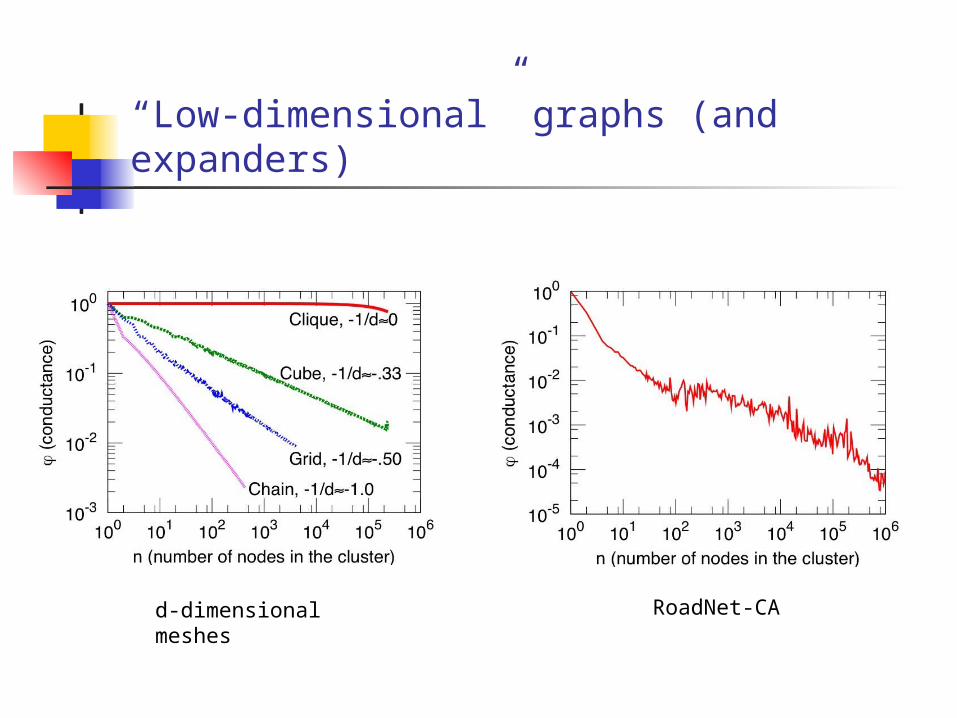
“Low-dimensional” graphs (and expanders)
d-dimensional meshes RoadNet-CA

NCPP for common generative models
Preferential Attachment Copying Model
RB Hierarchical Geometric PA

What do large networks look like?
Downward sloping NCPP
small social networks (validation)
“low-dimensional” networks (intuition)
hierarchical networks (model building)
existing generative models (incl. community models)
Natural interpretation in terms of isoperimetry
implicit in modeling with low-dimensional spaces, manifolds, k-means, etc.
Large social/information networks are very very different
We examined more than 70 large social and information networks
We developed principled methods to interrogate large networks
Previous community work: on small social networks (hundreds, thousands)
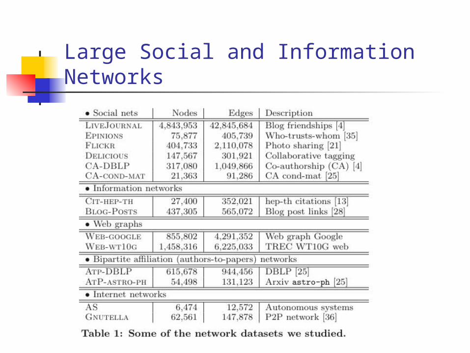
Large Social and Information Networks

Typical example of our findings
General relativity collaboration network (4,158 nodes, 13,422 edges)
51Community size
Com
munit
y s
core
Leskovec, Lang, Dasgupta, and Mahoney (WWW 2008 & arXiv 2008)

Large Social and Information Networks
LiveJournal Epinions
Focus on the red curves (local spectral algorithm) - blue (Metis+Flow), green (Bag of whiskers), and black (randomly rewired network) for consistency and cross-validation.
Leskovec, Lang, Dasgupta, and Mahoney (WWW 2008 & arXiv 2008)

More large networks
Cit-Hep-Th Web-Google
AtP-DBLP Gnutella

NCPP: LiveJournal (N=5M, E=43M)C
om
mu
nit
y s
core
Community size
Better and better
communitiesBest communities get
worse and worse
Best community has ≈100
nodes
54

Comparison with “Ground truth” (1 of 2)
Networks with “ground truth” communities:
• LiveJournal12: • users create and explicitly join on-line groups
• CA-DBLP: • publication venues can be viewed as communities
• AmazonAllProd: • each item belongs to one or more hierarchically organized categories, as defined by Amazon
• AtM-IMDB: • countries of production and languages may be viewed as communities (thus every movie belongs to exactly one community and actors belongs to all communities to which movies in which they appeared belong)

Comparison with “Ground truth” (2 of 2)
LiveJournal CA-DBLP
AmazonAllProd AtM-IMDB

Small versus Large NetworksLeskovec, et al. (arXiv 2009); Mahdian-Xu 2007
Small and large networks are very different:
0.99 0.55
0.55 0.15
0.99 0.17
0.17 0.82K1 =
E.g., fit these networks to Stochastic Kronecker Graph with “base” K=[a b; b c]:
0.2 0.2
0.2 0.2
(also, an expander)

Small versus Large NetworksLeskovec, et al. (arXiv 2009); Mahdian-Xu 2007
Small and large networks are very different:
K1 =
E.g., fit these networks to Stochastic Kronecker Graph with “base” K=[a b; b c]:
(also, an expander)

Some more thoughts ...
What I just described is “obvious” ...• There are good small clusters
• There are no good large clusters
... but not “obvious enough” that analysts don’t assume otherwise when deciding what algorithms to use
• k-means - basically the SVD
• Spectral normalized-cuts - appropriate when SVD is
• Recursive partitioning - recursion depth is BAD if you nibble off 100 nodes out of 100,000,000 at each step

Real large-scale applications
A lot of work on large-scale data already implicitly uses variants of these ideas:• Fuxman, Tsaparas, Achan, and Agrawal (2008): random walks on query-click for automatic keyword generation
• Najork, Gallapudi, and Panigraphy (2009): carefully “whittling down” neighborhood graph makes SALSA faster and better
• Lu, Tsaparas, Ntoulas, and Polanyi (2010): test which page-rank-like implicit regularization models are most consistent with data
These and related methods are often very non-robust
• basically due to the structural properties described,
• since the data are different than the story you tell.

Implications more generally
Empirical results demonstrate:
• (Good and large) network clusters, at least when formalized i.t.o. the inter-versus-intra bicriterion, don’t really exist in these graphs.
• To the extent that they barely exist, existing tools are designed not to find them.
This may be “obvious,” but not really obvious enough ...
• Algorithmic tools people use, models people develop, intuitions that get encoded in seemingly-minor design decisions all assume otherwise
Drivers, e.g., funding, production, bonuses, etc bias toward “positive” results
• Finding false positives is only going to get worse as the data get bigger.

Conclusions (and take-home lessons)
1. Matrices and graphs are basic structures for modeling data, and many algorithms boil down to matrix/graph algorithms.
2. Often, algorithms work when they “shouldn’t,” don’t work when they “should,” and interpretation is tricky but often of interest downstream.
3. Analysts tell stories since they often have no idea of what the data “look like,” but algorithms can be used to “explore” or “probe” the data.
4. Large networks (and large data) are typically very different than small networks (and small data), but people typically implicitly assume they are the same.


