
ORNL/TM-2017/289 CRADA/NFE-11-03242
Low Global Warming Potential Refrigerants for Commercial Refrigeration Systems
Brian A. Fricke Vishaldeep Sharma Omar Abdelaziz
June 2017
CRADA FINAL REPORT
NFE-11-03242
Approved for Public Release.
Distribution is Unlimited.
DOCUMENT AVAILABILITY
Reports produced after January 1, 1996, are generally available free via US Department of Energy (DOE) SciTech Connect. Website http://www.osti.gov/scitech/ Reports produced before January 1, 1996, may be purchased by members of the public from the following source: National Technical Information Service 5285 Port Royal Road Springfield, VA 22161 Telephone 703-605-6000 (1-800-553-6847) TDD 703-487-4639 Fax 703-605-6900 E-mail [email protected] Website http://www.ntis.gov/help/ordermethods.aspx Reports are available to DOE employees, DOE contractors, Energy Technology Data Exchange representatives, and International Nuclear Information System representatives from the following source: Office of Scientific and Technical Information PO Box 62 Oak Ridge, TN 37831 Telephone 865-576-8401 Fax 865-576-5728 E-mail [email protected] Website http://www.osti.gov/contact.html
This report was prepared as an account of work sponsored by an agency of the United States Government. Neither the United States Government nor any agency thereof, nor any of their employees, makes any warranty, express or implied, or assumes any legal liability or responsibility for the accuracy, completeness, or usefulness of any information, apparatus, product, or process disclosed, or represents that its use would not infringe privately owned rights. Reference herein to any specific commercial product, process, or service by trade name, trademark, manufacturer, or otherwise, does not necessarily constitute or imply its endorsement, recommendation, or favoring by the United States Government or any agency thereof. The views and opinions of authors expressed herein do not necessarily state or reflect those of the United States Government or any agency thereof.
i
ORNL/TM-2017/289
CRADA/NFE-11-03242
Building Technologies Research and Integration Center
LOW GLOBAL WARMING POTENTIAL REFRIGERANTS FOR COMMERCIAL
REFRIGERATION SYSTEMS
Brian A. Fricke
Vishaldeep Sharma
Omar Abdelaziz
Date Published: June 2017
Prepared by
OAK RIDGE NATIONAL LABORATORY
Oak Ridge, Tennessee 37831-6283
managed by
UT-BATTELLE, LLC
for the
US DEPARTMENT OF ENERGY
under contract DE-AC05-00OR22725
Approved for Public Release

ii

iii
CONTENTS
CONTENTS ................................................................................................................................................. iii LIST OF FIGURES ...................................................................................................................................... v LIST OF TABLES ...................................................................................................................................... vii ACRONYMS ............................................................................................................................................... ix EQUATION NOMENCLATURE ............................................................................................................... xi ACKNOWLEDGEMENTS ....................................................................................................................... xiii ABSTRACT ................................................................................................................................................ xv 1. INTRODUCTION .................................................................................................................................. 1
1.1 BACKGROUND .......................................................................................................................... 1 1.1.1 Refrigerant Development ................................................................................................. 1 1.1.2 Refrigerant Characteristics ............................................................................................... 1 1.1.3 Commercial Refrigeration ................................................................................................ 3
1.2 PROJECT OBJECTIVES ............................................................................................................. 4 1.3 MOTIVATION ............................................................................................................................. 4 1.4 OUTLINE OF REPORT .............................................................................................................. 5
2. LIFE CYCLE CLIMATE PERFORMANCE ........................................................................................ 7 2.1 EMISSIONS CALCULATIONS.................................................................................................. 9
2.1.1 Direct Emissions .............................................................................................................. 9 2.1.2 Indirect Emissions .......................................................................................................... 10
2.2 LCCP FRAMEWORK ............................................................................................................... 12 2.3 LCCP DESIGN TOOL ............................................................................................................... 13
2.3.1 Desktop LCCP Design Tool ........................................................................................... 14 2.3.2 Web-based LCCP Design Tool ...................................................................................... 17
3. LCCP ANALYSIS OF REFRIGERATION SYSTEMS...................................................................... 21 3.1 ENERGY MODELING .............................................................................................................. 21 3.2 REFRIGERATION SYSTEMS .................................................................................................. 23
3.2.1 Multiplex Direct Expansion (DX) System (S1) ............................................................. 23 3.2.2 Cascade/Secondary Loop System (S2) using R-448A and CO2 .................................... 24 3.2.3 Transcritical R-744 (CO2) Booster System (S3) ............................................................ 25 3.2.4 Secondary (MT) / Central DX (LT) System (S4) ........................................................... 27 3.2.5 Refrigeration System Modeling Assumptions ............................................................... 27
3.3 RESULTS AND DISCUSSION ................................................................................................. 29 3.3.1 LCCP Analysis ............................................................................................................... 29 3.3.2 Effect of Annual Refrigerant Leak Rate......................................................................... 32 3.3.3 Effect of Refrigerant Charge or Hourly Emission Rate for Electricity Production........ 32 3.3.4 Uncertainty Analysis ...................................................................................................... 33
3.4 SUMMARY................................................................................................................................ 35 4. LABORATORY EVALUATION OF ALTERNATIVE REFRIGERANTS ...................................... 37
4.1 COMMERCIAL REFRIGERATION SYSTEM DESCRIPTION ............................................. 37 4.1.1 Compressor Rack ........................................................................................................... 38 4.1.2 Refrigerated Display Cases ............................................................................................ 40 4.1.3 Air-Cooled Condenser ................................................................................................... 41 4.1.4 Refrigeration System Controls ....................................................................................... 42 4.1.5 Instrumentation .............................................................................................................. 42
4.2 TEST PLAN ............................................................................................................................... 43 4.2.1 Data Acquisition ............................................................................................................. 44 4.2.2 Data Analysis ................................................................................................................. 44
4.3 RESULTS ................................................................................................................................... 45

iv
4.3.1 Performance with Reciprocating Compressors .............................................................. 45 4.3.2 Summary of Results with Reciprocating Compressors .................................................. 50 4.3.3 Performance with Scroll Compressors ........................................................................... 50 4.3.4 Summary of Results with Scroll Compressors ............................................................... 55 4.3.5 Discussion ...................................................................................................................... 55
5. FIELD EVALUATION OF ALTERNATIVE REFRIGERANTS IN A COMMERCIAL
REFRIGERATION SYSTEM .................................................................................................................... 57 5.1 DESCRIPTION .......................................................................................................................... 57 5.2 DATA ACQUISITION .............................................................................................................. 58 5.3 FIELD EVALUATION REPORT .............................................................................................. 58 5.4 SITE SELECTION ..................................................................................................................... 58
6. CONCLUSIONS .................................................................................................................................. 61 7. REFERENCES ..................................................................................................................................... 63
v
LIST OF FIGURES
Figure Page
1. Framework for open-source LCCP computer algorithm. ........................................................ 13 2. Desktop LCCP Design Tool main input window. ................................................................... 14 3. Application Information input window. .................................................................................. 15 4. Simulation Information input window. ................................................................................... 16 5. Load Information input window. ............................................................................................. 16 6. Desktop LCCP Design Tool results window. .......................................................................... 17 7. Web-based LCCP Design Tool data input screen. .................................................................. 18 8. Web-based LCCP Design Tool data output screen. ................................................................ 19 9. EnergyPlus supermarket model. .............................................................................................. 22 10. Multiplex direct expansion (DX) refrigeration system (System S1). ...................................... 24 11. Cascade/secondary loop system (System S2) using R-448A and CO2. ................................... 25 12. Transcritical R-744 (CO2) booster refrigeration system (System S3). .................................... 26 13. Secondary (MT) / central DX (LT) refrigeration system (System S4). ................................... 27 14. Total direct emissions from the four refrigeration systems. .................................................... 30 15. Total indirect emissions and annual electricity consumption for the four refrigeration
systems. ................................................................................................................................... 31 16. Total emissions (direct and indirect) from the four refrigeration systems. ............................. 31 17. Effect of refrigerant leak rate on total CO2e emissions. ........................................................... 32 18. Sensitivity of total CO2e emissions due to a 10% increase in refrigerant charge. ................... 33 19. Sensitivity of total CO2e emissions due to a 10% increase in electricity production
emissions. ................................................................................................................................ 33 20. Schematic of laboratory-scale commercial refrigeration system. ........................................... 37 21. Compressor rack. ..................................................................................................................... 38 22. Low-temperature (a) and medium-temperature (b) display cases. .......................................... 40 23. Air-cooled condenser (top) mounted above liquid receiver (bottom). .................................... 41 24. Total system capacity for R-448A and R-404A, using reciprocating compressors. ............... 46 25. Total compressor power for R-448A and R-404A, using reciprocating compressors. ........... 46 26. Refrigeration system COP for R-448A and R-404A, using reciprocating compressors. ........ 47 27. Total refrigerant mass flow for R-448A and R-404A, using reciprocating compressors. ....... 47 28. Low-temperature (LT) and medium-temperature (MT) compressor isentropic efficiencies
for R-448A and R-404A, using reciprocating compressors. ................................................... 48 29. Low-temperature (LT) and medium-temperature (MT) compressor discharge temperatures
for R-448A and R-404A, using reciprocating compressors. ................................................... 49 30. Low-temperature (LT) and medium-temperature (MT) suction header pressures for R-448A
and R-404A, using reciprocating compressors. ....................................................................... 49 31. Low-temperature (LT) and medium-temperature (MT) display case discharge air
temperatures for R-448A and R-404A, using reciprocating compressors. .............................. 50 32. Total system capacity for R-448A and R-404A, using scroll compressors. ............................ 51 33. Total compressor power for R-448A and R-404A, using scroll compressors. ........................ 51 34. Refrigeration system COP for R-448A and R-404A, using scroll compressors. .................... 52 35. Total refrigerant mass flow for R-448A and R-404A, using scroll compressors. ................... 52 36. Low-temperature (LT) and medium-temperature (MT) compressor isentropic efficiencies
for R-448A and R-404A, using scroll compressors. ............................................................... 53 37. Low-temperature (LT) and medium-temperature (MT) compressor discharge temperatures
for R-448A and R-404A, using scroll compressors. ............................................................... 54

vi
38. Low-temperature (LT) and medium-temperature (MT) suction header pressures for R-448A
and R-404A, using scroll compressors. ................................................................................... 54

vii
LIST OF TABLES
Table Page
1. Commonly used refrigerants by application .............................................................................. 3 2. GWP values for selected refrigerants (IPCC 2013; UNEP 2010c) ........................................... 8 3. Material manufacturing emissions (IIR 2016) ........................................................................ 12 4. Refrigerant manufacturing emissions (IIR 2016) .................................................................... 12 5. Refrigerated display case specifications used in supermarket energy modeling
(Beshr et al. 2015) ................................................................................................................... 22 6. Refrigerated walk-in cooler/freezer specifications used in supermarket energy modeling
(Beshr et al. 2015) ................................................................................................................... 23 7. Climate zones and cities used in the LCCP analysis ............................................................... 23 8. Multiplex DX refrigeration system configuration (System S1) (Beshr et al. 2015) ................ 24 9. Cascade/secondary loop system (System S2) using R-448A and R-744 (Beshr et al. 2015) .. 25 10. Transcritical R-744 (CO2) booster refrigeration system configuration (System S3)
(Beshr et al. 2015) ................................................................................................................... 26 11. Secondary (MT) / central DX (LT) refrigeration system configuration (System S4)
(Beshr et al. 2015) ................................................................................................................... 27 12. Evaporating temperatures for the three refrigeration systems ................................................. 28 13. Refrigerant composition and GWP values (ASHRAE 2016; IPCC 2013) .............................. 29 14. Summary of uncertainty in LCCP parameters ......................................................................... 34 15. Uncertainties in the total CO2e emissions of the multiplex DX system (S1) ........................... 35 16. Partial derivatives of the total emissions with respect to each of the input parameters .......... 35 17. Compressor specifications for laboratory-scale refrigeration system ..................................... 39 18. Compressor rack capacity for laboratory-scale refrigeration system ...................................... 39 19. Refrigerated display case specifications .................................................................................. 41 20. Instrumentation specifications ................................................................................................. 42 21. Refrigeration system setpoints and operating conditions when operating with reciprocating
compressors ............................................................................................................................. 43 22. Refrigeration system setpoints and operating conditions when operating with scroll
compressors ............................................................................................................................. 44 23. Refrigeration rack specifications at field site .......................................................................... 59

viii

ix
ACRONYMS
AHRI Air-Conditioning, Heating and Refrigeration Institute
AHRTI Air-Conditioning, Heating and Refrigeration Technology Institute
ANSI American National Standards Institute
ASHRAE American Society of Heating, Refrigerating and Air-Conditioning Engineers
BTO Building Technologies Office (DOE)
CEC California Energy Commission
CFC chlorofluorocarbon
COP coefficient of performance
CO2 carbon dioxide
CO2e carbon dioxide equivalent
DOE U.S. Department of Energy
DTIE Division of Technology, Industry and Economics (UNEP)
DX direct expansion
EERE Energy Efficiency and Renewable Energy (DOE)
EPA U.S. Environmental Protection Agency
EPR evaporator pressure regulator
GHG greenhouse gas
GWP global warming potential
HCFC hydrochlorofluorocarbon
HFC hydrofluorocarbon
HFO hydrofluoro-olefin
HVAC&R heating, ventilating, air-conditioning and refrigeration
IIR International Institute of Refrigeration
IPCC Intergovernmental Panel on Climate Change
LCCP life cycle climate performance
LCWI life cycle warming impact
LT low-temperature
MAC mobile air-conditioning
MT medium-temperature
MTG multi-disciplinary task group
NREL National Renewable Energy Laboratory
ODP ozone depleting potential
ORNL Oak Ridge National Laboratory
PNNL Pacific Northwest National Laboratory
RH relative humidity
ROI return on investment
TEWI total equivalent warming impact
TMY typical meteorological year
UNEP United Nations Environment Program

x
xi
EQUATION NOMENCLATURE
𝐶𝑂𝑃 coefficient of performance
𝑒𝑒𝑙𝑒𝑐 carbon dioxide emission factor associated with the generation and distribution of the
electrical energy used to power the refrigeration system (kg CO2e/kWh)
𝑒𝑟𝑒𝑓,𝐸𝑂𝐿 carbon dioxide emission factor associated with the disposal of the refrigerant at the end-
of-life of the system (kg CO2e/kg)
𝑒𝑟𝑒𝑓,𝑚𝑎𝑛 carbon dioxide emission factor associated with the manufacture of the refrigerant
(kg CO2e/kg)
𝑒𝑠𝑦𝑠,𝐸𝑂𝐿 carbon dioxide emission factor associated with the disposal of a particular material at the
end-of-life of the system (kg CO2e/kg)
𝑒𝑠𝑦𝑠,𝑚𝑎𝑛 carbon dioxide emission factor associated with the manufacture of that particular material
(kg CO2e/kg)
𝐸 annual electrical energy consumption of the refrigeration system (kWh)
𝐸𝑎𝑐𝑐𝑖𝑑 total carbon dioxide equivalent emissions due to refrigerant release caused by accidents
(kg CO2e)
𝐸𝑑𝑖𝑟𝑒𝑐𝑡 direct emission
𝐸𝑒𝑙𝑒𝑐 emission associated with the generation of electricity used to power the refrigeration
system over its operating lifetime (kg CO2e)
𝐸𝐸𝑂𝐿 total carbon dioxide equivalent emissions due to refrigerant release at the end-of-life of
the system (kg CO2e)
𝐸𝑖𝑛𝑑𝑖𝑟𝑒𝑐𝑡 indirect emission
𝐸𝑙𝑒𝑎𝑘 total carbon dioxide equivalent emissions due to annual refrigerant leakage from the
system over its operating lifetime (kg CO2e)
𝐸𝑟𝑒𝑓,𝐸𝑂𝐿 emission associated with the energy to dispose of the refrigerant at the end-of-life of the
system (kg CO2e)
𝐸𝑟𝑒𝑓,𝑚𝑎𝑛 emission associated with the energy to manufacture the refrigerant (kg CO2e)
𝐸𝑠𝑒𝑟𝑣𝑖𝑐𝑒 total carbon dioxide equivalent emissions due to refrigerant release during servicing
events, over the operating lifetime of the system (kg CO2e)
𝐸𝑠𝑦𝑠,𝐸𝑂𝐿 emission associated with the energy to dispose of the refrigeration system components at
the end-of-life of the system (kg CO2e)
𝐸𝑠𝑦𝑠,𝑚𝑎𝑛 emissions associated with the energy to manufacture the refrigeration system (kg CO2e)
𝐺𝑊𝑃 global warming potential of the refrigerant (kg CO2e/kg)
𝐺𝑊𝑃𝑎𝑑𝑝 global warming potential of the atmospheric degradation products of the refrigerant
(kg CO2e/kg)
ℎ𝑐,𝑖𝑛 average compressor inlet enthalpy determined from measured refrigerant temperature and
pressure
ℎ𝑐,𝑜𝑢𝑡,𝑠 average compressor outlet enthalpy assuming isentropic compression between the inlet
and outlet pressures
ℎ𝑖,𝑖𝑛 average refrigerant enthalpy at the inlet of load i
ℎ𝑖,𝑜𝑢𝑡 average refrigerant enthalpy at the exit of load i
𝐿 lifetime of the system (in years)
𝐿𝐶𝐶𝑃 total CO2e emissions
𝑚𝑐 total refrigerant charge in the system (kg)
�̇�𝑖 average refrigerant mass flow through load i
𝑚𝑠𝑦𝑠 mass of a particular material used in the construction of the refrigeration system (kg)
�̇�𝑖 average refrigeration capacity for load i
�̇�𝑡𝑜𝑡𝑎𝑙 average total refrigeration capacity

xii
�̇�𝑖,𝐿𝑇 average input power to low-temperature compressor i
�̇�𝑗,𝑀𝑇 average input power to medium-temperature compressor j
�̇�𝑡𝑜𝑡𝑎𝑙 average total compressor power
𝑥𝑎𝑐𝑐𝑖𝑑 annual refrigerant loss during accidents (in fraction of total refrigerant charge per year)
𝑥𝐸𝑂𝐿 refrigerant loss occurring at the end-of-life decommissioning of the system (in fraction of
total refrigerant charge)
𝑥𝑙𝑒𝑎𝑘 annual refrigerant leak rate (in fraction of total refrigerant charge per year)
𝑥𝑟𝑒𝑢𝑠𝑒 fraction of the refrigerant in the system which is reclaimed refrigerant
𝑥𝑠𝑒𝑟𝑣𝑖𝑐𝑒 annual refrigerant loss during service events (in fraction of total refrigerant charge per
year)
𝜂𝑖,𝑡ℎ average isentropic efficiency of the ith compressor

xiii
ACKNOWLEDGEMENTS
This report and the work described were sponsored by the Emerging Technologies Program within the
Building Technologies Office (BTO) of the US Department of Energy (DOE) Office of Energy Efficiency
and Renewable Energy. The authors wish to acknowledge the support of Antonio Bouza in guiding this
work. A special debt of gratitude is due to Michael Petersen, Gustavo Pottker, Ankit Sethi and Samuel
Yana Motta of Honeywell, as well as Vikrant Aute, Mohamed Beshr and Reinhard Radermacher at the
University of Maryland, for without their contributions, this project would not have been a success.
Finally, this work would not have been possible without the outstanding technical support provided by
Brian Goins, Randy Linkous, Geoffrey Ormston, Jeffrey Taylor and Marty Zorn.

xiv

xv
ABSTRACT
Supermarket refrigeration systems account for approximately 50% of supermarket energy use,
placing this class of equipment among the highest energy consumers in the commercial building domain.
In addition, the commonly used refrigeration system in supermarket applications is the multiplex direct
expansion (DX) system, which is prone to refrigerant leaks due to its long lengths of refrigerant piping.
This leakage reduces the efficiency of the system and increases the impact of the system on the
environment. The high Global Warming Potential (GWP) of the hydrofluorocarbon (HFC) refrigerants
commonly used in these systems, coupled with the large refrigerant charge and the high refrigerant
leakage rates leads to significant direct emissions of greenhouse gases into the atmosphere.
Environmental concerns are driving regulations for the heating, ventilating, air-conditioning and
refrigeration (HVAC&R) industry towards lower GWP alternatives to HFC refrigerants. Existing lower
GWP refrigerant alternatives include hydrocarbons, such as propane (R-290) and isobutane (R-600a), as
well as carbon dioxide (R-744), ammonia (R-717), and R-32. In addition, new lower GWP refrigerant
alternatives are currently being developed by refrigerant manufacturers, including hydrofluoro-olefin
(HFO) and unsaturated hydrochlorofluorocarbon (HCFO) refrigerants.
The selection of an appropriate refrigerant for a given refrigeration application should be based on
several factors, including the GWP of the refrigerant, the energy consumption of the refrigeration system
over its operating lifetime, and leakage of refrigerant over the system lifetime. For example, focusing on
energy efficiency alone may overlook the significant environmental impact of refrigerant leakage; while
focusing on GWP alone might result in lower efficiency systems that result in higher indirect impact over
the equipment lifetime.
Thus, the objective of this Collaborative Research and Development Agreement (CRADA) between
Honeywell and the Oak Ridge National Laboratory (ORNL) is to develop a Life Cycle Climate
Performance (LCCP) modeling tool for optimally designing HVAC&R equipment with lower life cycle
greenhouse gas emissions, and the selection of alternative working fluids that reduce the greenhouse gas
emissions of HVAC&R equipment. In addition, an experimental evaluation program is used to measure
the coefficient of performance (COP) and refrigerating capacity of various refrigerant candidates, which
have differing GWP values, in commercial refrigeration equipment. Through a cooperative effort between
industry and government, alternative working fluids will be chosen based on maximum reduction in
greenhouse gases at minimal cost impact to the consumer. This project will ultimately result in advancing
the goals of reducing greenhouse gas emissions through the use of low GWP working fluids and
technologies for HVAC&R and appliance equipment, resulting in cost-competitive products and systems.
An LCCP methodology is presented to determine the direct and indirect emissions associated with the
lifetime operation of refrigeration systems, from system construction through system operation and
system dismantling. The methodology is incorporated into an open-source LCCP Design Tool which can
be used to estimate the lifetime direct and indirect carbon dioxide equivalent gas emissions of various
commercial refrigeration system designs and refrigerant options, with the goal of providing guidance on
lower GWP refrigerant solutions with improved LCCP compared to baseline systems. The LCCP Design
Tool is available in a desktop computer version and a simplified web-based version. Both versions may
be accessed from http://lccp.umd.edu/.
The open-source LCCP Design Tool is used to compare the lifetime emissions of four commercial
refrigeration system configurations, using four refrigerants (R-404A, R-448A, R-744 [CO2], and L-40), in
six US cities representing different climate zones. The four refrigeration systems include the multiplex
direct expansion (DX) system, the cascade/secondary loop system, the transcritical CO2 booster system,
and the medium-temperature secondary loop/low-temperature DX system. Finally, a sensitivity analysis
is performed to identify the relative importance of various input parameters on the calculated total CO2
equivalent emissions of supermarket refrigeration systems.
Comparing the total emissions for different cities suggests that the transcritical CO2 booster system
has the lowest CO2 equivalent emissions, according to this analysis, in cold and temperate climates. Also,

xvi
the R-448A/L-40 secondary circuit refrigeration system was found to offer a good balance between
emissions and electricity consumption for hot climates. The parametric analysis showed that shifting
towards low GWP refrigerants decreases the effect of the annual leak rate on the total system emissions.
Moreover, the sensitivity analysis showed that shifting towards low GWP refrigerants, or more charge
conservative systems increases the effect of the hourly emission rate for electricity production on the total
system emissions. Finally, an uncertainty analysis was performed showing that using low GWP
refrigerants, or more charge conservative systems causes a noticeable drop in the impact of the
uncertainty in the inputs related to the direct emissions.
The energy performance of an alternative lower global warming potential refrigerant, R-448A, was
evaluated in a laboratory-scale commercial refrigeration system, and its performance was compared to
that of the commonly used higher GWP refrigerant, R-404A, found in the commercial refrigeration
industry. The laboratory-scale commercial refrigeration system installed in the environmental test
chambers at ORNL consists of components typically found in most U.S. supermarket refrigeration
systems, including a compressor rack, an air-cooled condenser and several medium-temperature (MT) and
low-temperature (LT) refrigerated display cases. The refrigeration system has a low-temperature cooling
capacity of approximately 5 tons at −20°F (18 kW at −29°C) and a medium-temperature cooling capacity
of approximately 10 to 15 tons at 25°F (35 to 53 kW at −4°C). The compressor rack of the commercial
refrigeration system is unique in that it contains two types of compressors that are commonly found in
supermarket refrigeration systems: reciprocating compressors and scroll compressors. Having both
reciprocating and scroll compressors allows for system performance tests to be performed using the two
common compressor types employed in supermarket refrigeration systems.
Using each refrigerant (R-404A and R-448A), the performance of the laboratory-scale commercial
refrigeration system was determined at four ambient temperature conditions: 60°F, 75°F, 95°F and 105°F
(16°C, 24°C, 35°C, and 41°C). It was found that R-448A and R-404A performed similarly in the
laboratory-scale commercial refrigeration system. Compared to R-404A, R-448A exhibited an energy
benefit since system COP was increased and compressor power was decreased. The refrigeration
capacity of R-448A was found to be similar to that of R-404A. For the same saturated evaporating and
condensing temperatures, compressor suction pressures of R-448A were lower than that of R-404A while
compressor discharge temperatures of R-448A were higher. Since system performance differences
between R-448A and R-404A are small, it can be presumed that R-448A would be a suitable drop-in
replacement refrigerant for R-404A. Only minor changes in the system would be required to retrofit
R-404A with R-448A. Suction pressure setpoints would need to be reduced and expansion valve
superheat settings would require adjustment.
Future efforts related to this project include completing a field evaluation of the lower GWP
alternative refrigerant in third-party supermarkets. The main objective of the field evaluation is to
compare the energy consumption of refrigeration systems using incumbent refrigerants and alternative
refrigerants in actual, operating supermarkets, thereby providing motivation to supermarket owners and
operators to retrofit existing systems with the lower GWP alternative. Honeywell and ORNL are
currently negotiating the site selection and logistics for the field evaluation of R-448A with a major food
retailer.
Motivated by the outstanding energy and environmental performance of the alternative lower GWP
refrigerant R-448A, the CRADA partner, Honeywell has commercialized the refrigerant (Solstice® N40)
as an alternative to R-404A in both new and existing commercial refrigeration systems.

1
1. INTRODUCTION
1.1 BACKGROUND
Mechanical vapor compression refrigeration cycles are used to move heat from one location to
another via a working fluid (i.e., the refrigerant). The refrigerant typically changes phase as it flows
around the refrigeration cycle. The refrigerant absorbs heat from one location, and in doing so, it
evaporates. Subsequently, the refrigerant rejects heat to another location, and is condensed during the
process. Vapor compression refrigeration cycles can be used for either of two purposes. A refrigeration
system is used to maintain a space at a lower temperature relative to the ambient temperature while a heat
pump system is used to maintain a space at a higher temperature relative to the ambient temperature.
1.1.1 Refrigerant Development
The first generation of vapor compression refrigeration systems manufactured in the latter half of the
19th century and the first quarter of the 20
th century utilized refrigerants that were both readily available
and found to produce the desired cooling effect. The refrigerants of that time included chemicals such as
sulfur dioxide, ethyl chloride, methyl chloride and ammonia, among others. However, these refrigerants
posed safety hazards due to their toxicity and/or flammability. Beginning in the 1930s,
chlorofluorocarbon (CFC) and hydrochlorofluorocarbon (HCFC) refrigerants were developed as safe,
nontoxic and nonflammable alternatives for the early refrigerants (Midgley and Henne 1930). In the
ensuing years, the application of CFCs and HCFCs expanded to include use as aerosol propellants,
cleaning agents for the microelectronics industry, and blowing agents for foam insulation. As a result, the
quantities of CFCs and HCFCs produced increased rapidly during the 1950s and 1960s.
Subsequently, in the 1970s, scientists discovered that CFC and HCFC refrigerants were contributing
to the depletion of the ozone in the earth’s stratosphere (Molina and Rowland 1974a, b). It was found that
the stability of the CFC and HCFC molecules cause them to remain in the atmosphere for a significant
time, and once these molecules migrate into the stratosphere, they dissociate and release chlorine atoms.
The chlorine atoms then react with ozone (O3) to produce diatomic oxygen (O2), thereby depleting the
ozone in the stratosphere.
In 1987, an international treaty, the Montreal Protocol on Substances that Deplete the Ozone Layer,
was ratified to protect the ozone layer by requiring the phase-out of numerous substances believed to be
responsible for ozone depletion. The Protocol sets a mandatory timetable for the phase out of ozone
depleting substances, including CFCs and HCFCs. In the United States, production and importation of
CFCs were banned completely in 1996. HCFCs are being phased down, with complete phase-out set for
2030 (ASHRAE 2013).
Following the proposed phase-out of ozone depleting refrigerants per the Montreal Protocol,
hydrofluorocarbon (HFC) refrigerants were introduced, and these refrigerants are in common use today.
HFC refrigerants contain no chlorine atoms, and thus, they have no ozone depleting potential (ODP).
However, HFC refrigerants typically have a high global warming potential (GWP), and thus, release of
HFCs into the atmosphere represents a notable source of greenhouse gases. Since HFCs have a high
GWP, there is strong interest to minimize the introduction and emissions of HFCs. Alternative
refrigerants with lower or near zero GWP are available including hydrocarbons such as propane (R-290)
and isobutane (R-600a), ammonia (R-717), carbon dioxide (R-744) and new hydrofluoro-olefin (HFO)
refrigerants such as R-1234yf and R-1234ze(E) (UNEP 2010a, b).
1.1.2 Refrigerant Characteristics
The preceding discussion regarding the evolution of refrigerants highlights just a few of the factors
affecting refrigerant selection, including safety concerns and environmental concerns. There are several
other factors which also influence the selection of refrigerants for specific refrigeration applications, and

2
the following list provides the properties that an ideal refrigerant should possess (ASHRAE 2013; Kuehn,
Ramsey, and Threlkeld 1998):
Latent heat of vaporization: The latent heat of vaporization of a refrigerant is directly related to
its refrigerating effect (i.e., its ability to absorb heat) per unit mass. Thus, it is desirable to use
refrigerants with a high latent heat of vaporization.
Heat transfer characteristics: In order to reduce the size of heat exchangers in refrigeration
systems, refrigerants should exhibit high heat transfer coefficients. Transport properties such as
thermal conductivity, viscosity and density impact the heat transfer characteristics of the
refrigerant.
Critical temperature: Refrigeration systems operate most efficiently when the temperature of the
refrigerant remains well below the critical temperature. The cooling capacity and heat rejection
of refrigerants with a low critical temperature are greatly reduced as the condensing temperature
approaches the critical temperature. In addition, power consumption increases significantly as the
system operates near the critical temperature. Thus, refrigerants with high critical temperatures
are preferred.
Evaporating pressure: To ensure that air and moisture do not enter the refrigeration system
through leaks in the system, the minimum operating pressure of the system (i.e., the evaporating
pressure) should always be greater than atmospheric pressure. If air and moisture are drawn into
the system through a leak, system performance will deteriorate. Non-condensable gases such as
air in the refrigerant can reduce cooling capacity and system efficiency. Moisture in the system
can react with refrigerants to form acids which lead to corrosion and “sludging” of lubricant.
Moisture in the refrigerant can also freeze at expansion devices, thereby blocking refrigerant
flow.
Condensing pressure: Since compressor energy consumption is a function of the difference
between condensing and evaporating pressures, a low condensing pressure is desired to reduce
compressor energy consumption. Also, since components on the high-pressure side of the
refrigeration system must withstand the operating pressures without failure, lower condensing
pressures require less massive components.
Inertness and stability: The refrigerant must be chemically inert and stable so as not react with
any of the materials within the system, including the metals used for piping and other
components, lubricants, plastic components, and elastomers in valves and fittings.
Oil solubility: The lubricating oil must have good miscibility and solubility with the refrigerant
so that the oil returns to the compressor and does not collect in other parts of the system.
Toxicity: Both the acute (short-term) and chronic (long-term) toxicity of a refrigerant should be
considered as they affect human safety during handling and servicing systems with refrigerants,
and for occupants in refrigerated or air conditioned spaces. Thus, refrigerants should be non-
toxic.
Flammability: Preferably, a refrigerant should be nonflammable and not burn or support
combustion in any concentration with atmospheric air.
Ozone depletion potential (ODP): The refrigerant should not contribute to the depletion of
atmospheric ozone, and thus should have zero ozone depletion potential.
Global warming potential (GWP): The refrigerant should not contribute to the greenhouse effect
or the global warming effect, and thus should have a low global warming potential.
Detection: The refrigerant should be easily detected by refrigerant gas leak detection equipment.
Cost: The refrigerant should be readily available at a low cost.
Low viscosity to ensure minimal pressure drop through the piping, heat exchangers, and other
components.
Currently, no single fluid satisfies all of the desirable attributes of an ideal refrigerant, and
consequently, a variety of refrigerants are used. Table 1 list the most widely used refrigerants by their
application.

3
Table 1. Commonly used refrigerants by application
Application Commonly used refrigerants
Domestic refrigeration R-134a
Commercial refrigeration R-404A, R-134a, R-744
Industrial refrigeration R-134a, R-404A, R-22, R-717
Transport refrigeration R-404A, R-134a
Mobile air-conditioning R-134a
Residential air-conditioning R-410A, R-407C
Commercial air-conditioning R-410A, R-407C
Chillers R-134a, R-410A, R-407C
Heat pumps for space heating and water heating R-410A, R-744
1.1.3 Commercial Refrigeration
In this project, attention will be focused on evaluating the greenhouse gas emissions associated with
the operation of commercial refrigeration systems, and selecting refrigerants for commercial refrigeration
applications which provide energy efficiency with reduced environmental impact.
The traditional multiplex direct expansion (DX) refrigeration system used in commercial applications
is prone to significant refrigerant leakage, especially for relatively older existing systems. The EPA
(2011) estimates that the U.S. supermarket industry-wide average refrigerant emission rate is
approximately 25%. The use of high GWP refrigerants in these systems, combined with high refrigerant
leakage, can result in considerable direct carbon dioxide equivalent (CO2e) emissions. In addition,
commercial refrigeration systems consume a substantial amount of electrical energy, resulting in high
indirect CO2e emissions. Thus, there are ongoing efforts to reduce the direct and indirect environmental
impacts of commercial refrigeration systems through the use of leak reduction measures, refrigerant
charge minimization, low GWP refrigerants and energy efficiency measures. An example of one such
effort to promote these measures in the U.S. is the EPA GreenChill program (EPA 2016). This voluntary
program is a partnership between the EPA and food retailers to reduce refrigerant emissions and to
decrease the environmental impact of commercial refrigeration systems. Partner stores in the GreenChill
program have annual refrigerant emission rates ranging from ~13-14%, or about half the U.S. average
(EPA 2016).
With the phase-out of chlorofluorocarbon (CFC) and hydrochlorofluorocarbon (HCFC) refrigerants,
manufacturers have turned to hydrofluorocarbons (HFC) as substitutes. The zero ozone-depleting
potential of HFCs is appealing; however, many have relatively high GWPs. Thus, environmental
concerns are driving regulations and the heating, ventilating, air-conditioning and refrigeration
(HVAC&R) industry towards lower GWP alternatives to HFC refrigerants. Existing lower GWP
refrigerant alternatives include hydrocarbons, such as propane (R-290) and isobutane (R-600a), as well as
carbon dioxide (R-744), ammonia (R-717), and R-32. Note that with the exception of carbon dioxide, all
of these existing alternatives are either mildly flammable (American Society of Heating, Refrigerating
and Air-Conditioning Engineers [ASHRAE] safety classification 2L for ammonia and R-32) or have
higher flammability (ASHRAE safety classification 3 for propane and isobutane). In addition to existing
alternatives, new lower GWP refrigerant alternatives are currently being developed by refrigerant
manufacturers, including hydrofluoro-olefin (HFO) and unsaturated hydrochlorofluorocarbon (HCFO)
refrigerants. These next-generation refrigerants and their blends are typically either non-flammable
(ASHRAE safety classification 1) or have lower flammability (ASHRAE safety classification A2L).
The selection of an appropriate refrigerant for a given refrigeration application should be based on
several factors, including the GWP of the refrigerant, the energy consumption of the refrigeration system

4
over its operating lifetime, and leakage of refrigerant over the system lifetime. For example, focusing on
energy efficiency alone may overlook the significant environmental impact of refrigerant leakage; while
focusing on GWP alone might result in lower efficiency systems that result in higher indirect impact over
the equipment lifetime.
1.2 PROJECT OBJECTIVES
The objective of this Collaborative Research and Development Agreement (CRADA) between
Honeywell and the Oak Ridge National Laboratory (ORNL) is to develop a Life Cycle Climate
Performance (LCCP) modeling tool for optimally designing HVAC&R equipment with lower life cycle
greenhouse gas emissions, and the selection of alternative working fluids that reduce the greenhouse gas
emissions from HVAC&R equipment. In addition, an experimental testing program will be utilized to
measure the COP and capacity of various refrigerant candidates, which have differing GWP values, in
commercial refrigeration equipment. Through a cooperative effort between industry and government,
alternative working fluids will be chosen based on maximum reduction in greenhouse gases at minimal
cost impact to the consumer. This project will ultimately result in advancing the goals of reducing
greenhouse gas emissions through the use of low GWP working fluids and technologies for HVAC&R
and appliance equipment, resulting in cost-competitive products and systems.
The CRADA partner, Honeywell, with established leadership in the development of refrigerants, will
develop alternative lower GWP refrigerants for refrigeration, air-conditioning, heat pump, and appliance
equipment. The LCCP tool development effort, performed in conjunction with the University of
Maryland, will recognize the current national (ASHRAE Multidisciplinary Task Group [MTG] on low
GWP refrigerants) and international (International Institute of Refrigeration [IIR] LCCP working party)
efforts to standardize the LCCP evaluation procedures as well as recognize the needs of the U.S.
HVAC&R stakeholders.
1.3 MOTIVATION
The Department of Energy’s (DOE) Building Technologies Office (DOE-BTO) has as its long term
goal to create marketable technologies and design approaches that address energy consumption in existing
and new buildings. The current vision that DOE-BTO has for achieving this goal involves reducing the
energy and carbon emissions used by the energy service equipment (i.e., equipment providing space
heating and cooling, water heating, etc.) by 50% compared to today’s best common practice. Alternative
refrigerants with low global warming potential are needed to achieve DOE’s goal of reducing carbon
emissions.
Hydrofluorocarbon refrigerants and their blends are essential to the operation of vapor compression
equipment which dominates the residential and commercial heating, ventilating, air-conditioning and
refrigeration market. As concerns about climate change intensify, it is becoming increasingly clear that
suitable alternative refrigerants which have a lower GWP compared to today’s commonly used
refrigerants will be needed. Previous research efforts by the DOE during the period when ozone
depletion was an issue resulted in DOE being a guiding force behind the selection of alternative
refrigerants. By taking an early lead in research regarding low GWP refrigerants, the DOE will again
have a primary role in determining which alternatives are selected.
Present research efforts by refrigerant suppliers are more focused on the manufacturing processes. In
addition, refrigerant suppliers have limited resources and equipment for testing. This project will provide
guidance to the HVAC&R community on selecting alternative, energy-efficient, low GWP refrigerants.
5
1.4 OUTLINE OF REPORT
The structure of this report is as follows:
Chapter 2 presents the development of the Life Cycle Climate Performance (LCCP)
methodology which is used to estimate the lifetime emissions associated with the
construction, operation and dismantling of refrigeration systems.
Chapter 3 presents an LCCP analysis of various refrigeration system designs and refrigerant
options.
Chapter 4 presents the performance evaluation of a laboratory-scale supermarket refrigeration
system using the traditional refrigerant, R-404A, and an alternative refrigerant option,
R-448A.
Chapter 5 outlines a planned field study in which the performance of an actual operating
supermarket refrigeration system is evaluated with its incumbent refrigerant and the
alternative refrigerant, R-448A.
Finally, Chapter 6 presents concluding remarks.

6

7
2. LIFE CYCLE CLIMATE PERFORMANCE
When energy from the sun reaches the Earth, roughly two-thirds of that solar energy is absorbed by
the Earth’s surface and the atmosphere, while the remaining one-third of the solar energy is reflected back
to space (IPCC 2007). In order to balance the incoming solar radiation which is absorbed by the Earth,
the Earth must radiate an equivalent amount of energy back to space. As the Earth re-emits radiation in
the infrared portion of the spectrum, a significant portion of that energy is absorbed by the atmosphere.
This phenomenon is referred to as the greenhouse effect, and it is due to the presence of greenhouse gases
in the atmosphere. Greenhouse gases are those gases that can absorb and emit radiation within the
thermal infrared range. Greenhouse gases (GHGs) in the earth’s atmosphere trap heat near the earth’s
surface, thereby maintaining the Earth’s surface temperature about 60°F warmer than would otherwise be
the case if these gases were not present (ASHRAE 2013). Increasing concentrations of GHGs can lead to
an increased warming of the Earth.
The most abundant greenhouse gases in Earth's atmosphere include water vapor (H2O), carbon
dioxide (CO2), methane (CH4), nitrous oxide (N2O) and ozone (O3). The atmospheric concentrations of
greenhouse gases are determined by the balance between sources (emissions of greenhouse gases from
human activities and natural systems) and sinks (the removal of greenhouse gases from the atmosphere by
conversion to different chemical compounds) (Becker 2013).
Different greenhouse gases absorb and trap varying amounts of infrared radiation. They also persist
in the atmosphere for differing time periods and influence atmospheric chemistry (especially the ozone) in
different ways. The global warming potential of a greenhouse gas depends on both the efficiency of the
molecule as a greenhouse gas and its atmospheric lifetime (EPA 2010).
The global warming potential of a GHG is an index describing its relative ability to trap radiant
energy compared to carbon dioxide (CO2), which has a very long atmospheric lifetime (ASHRAE 2013).
Quantification of the climate impact of refrigerant emissions is thus often reported in CO2 equivalent
emissions (CO2e). GWP may be calculated for any particular integration time horizon (ITH). Typically, a
100-year ITH is used for regulatory purposes, and may be designated as GWP100 (ASHRAE 2013).
Many refrigerants, such as CFCs, HCFCs, HFCs, hydrocarbons and carbon dioxide, are greenhouse
gases. Newly developed hydrofluoro-olefin (HFO) refrigerants and their blends are being promoted as
lower-GWP alternatives to existing HCFC and HFC refrigerants. These HFOs are also GHGs, but their
GWPs are significantly lower than those of HCFCs and HFCs (ASHRAE 2013). Depending upon the
specific refrigeration application, direct release of refrigerant into the atmosphere can be a significant
source of greenhouse gases. Table 2 lists the GWP values of several common refrigerants.
One source of greenhouse gas emissions associated with the operation of refrigeration systems is
direct release of refrigerant from these systems to the atmosphere. Large field-erected refrigeration
systems, such as those found in supermarkets or refrigerated warehouses, contain may joints, fittings and
components which are prone to leakage over time. This refrigerant leakage can be significant, releasing
as much as 25% of the total refrigerant charge per year. On the other hand, small refrigeration systems
such as those found in domestic refrigerators, window air conditioners, and beverage vending machines
for example, are factory-sealed with only a few fittings and components, resulting in little or no
refrigerant leakage over their operating lifetime. The major source of refrigerant emissions for sealed
systems occurs at the end-of-life when refrigerant is recovered from the systems. Invariably, some
refrigerant is lost to the atmosphere during the recovery process.
Another source of greenhouse gas emissions associated with refrigeration system operation is related
to the electrical energy consumed by the systems. The electrical energy that refrigeration systems
consume is typically produced from fossil-fuel-fired power plants. The production of this electrical
energy results in the emission of CO2 due to the combustion of the fossil fuel. Depending upon the
specific refrigeration application, the indirect greenhouse gas emission associated with energy generation
can frequently be much larger than the direct emission due to refrigerant release. Such is the case with
small, factory-sealed refrigeration units which exhibit little or no refrigerant leakage over their operating

8
lifetimes. Nearly all of the greenhouse gas emissions for these systems is associated with the electrical
energy generation used to power these systems. On the other hand, for larger field-erected systems such
as supermarket refrigeration systems, direct emissions due to refrigerant leakage and indirect emissions
due to energy generation can equally contribute to the overall lifetime greenhouse gas emissions of these
systems.
Table 2. GWP values for selected refrigerants
(IPCC 2013; UNEP 2010c)
Refrigerant GWP (kg CO2e/kg)
R-22 1760
R-32 677
R-123 79
R-125 3170
R-134a 1300
R-143a 4800
R-152a 138
R-290 (propane) 3
R-404A 3943
R-410A 1924
R-600a (isobutane) 4
R-717 (ammonia) 0
R-744 (carbon dioxide) 1
R-1234yf <1
R-1234ze(E) <1
Several concepts are often used to evaluate the overall lifetime greenhouse gas impact of refrigeration
systems, including the Total Equivalent Warming Impact (TEWI), Life Cycle Climate Performance
(LCCP), and Life Cycle Warming Impact (LCWI). These concepts are similar in that they sum the total
equivalent direct and indirect greenhouse gas emissions from the refrigeration system, over the lifetime of
the system. These concepts are often used to compare different technologies to identify which
components should be optimized to effectively reduce global warming. These measures of global
warming include the carbon dioxide production resulting from the generation of electrical energy to
operate the refrigeration system plus the influence of the refrigerant itself if released into the atmosphere.
Consequently, they include the energy efficiency of the refrigeration system.
The Total Equivalent Warming Impact (TEWI) is an index which includes the effects of CO2
production due to the energy use of the refrigeration system and the effects of the release of refrigerant
over the useful life of the refrigeration system. The warming impact associated with CO2 emissions due
to energy use are referred to as indirect effects while the warming impact due to the release of refrigerant
is referred to as direct effects (Lommers 2002). The total effect on the environment must be given for a
period of time, which is typically 100 years (Baxter, Fischer, and Sand 1998).
The TEWI for a refrigeration system can be estimated from the total amount of refrigerant released
during the lifetime of operation of the system and the total energy used by the refrigeration system over
its useful lifetime as follows:
𝑇𝐸𝑊𝐼 = (�̇�𝑟𝑒𝑓𝑟𝑖𝑔)(𝐺𝑊𝑃𝑟𝑒𝑓𝑟𝑖𝑔) + 𝛼𝐸𝑎𝑛𝑛𝑢𝑎𝑙𝐿 (1)
where �̇�𝑟𝑒𝑓𝑟𝑖𝑔 is the mass of refrigerant released over the useful life of the system, 𝐺𝑊𝑃𝑟𝑒𝑓𝑟𝑖𝑔 is the
global warming potential of the refrigerant, 𝛼 is a conversion of energy use into CO2 emissions, 𝐸𝑎𝑛𝑛𝑢𝑎𝑙
9
is the annual energy usage of the system and 𝐿 is the useful life of the system, in years (Baxter, Fischer,
and Sand 1998).
Life Cycle Climate Performance (LCCP) is a method to determine the environmental impact of
refrigeration system design, refrigerant selection and system operation over the operating lifetime of the
refrigeration system, from system construction through system operation to system dismantling. The
environmental impact of the refrigeration system is measured by estimating the system’s greenhouse gas
emissions in terms of carbon dioxide equivalent emissions. The carbon dioxide equivalent emission is the
quantity of carbon dioxide that would have the same GWP as the greenhouse gas emissions of the
refrigeration system under consideration (Hafner, Nekså, and Pettersen 2004; Horie et al. 2010; Johnson
2004; Papasavva, Hill, and Andersen 2010; Spatz and Yana Motta 2004; Zhang et al. 2011).
The LCCP concept has been used to compare the overall environmental impact of selected HFCs to
other fluids and technologies in applications such as automobile air conditioning, residential and
commercial refrigeration, unitary air conditioning, and chillers (ADL 2002). In addition, some tools for
system evaluation based on LCCP have been presented in the literature. Papasavva, Hill, and Andersen
(2010) developed a comprehensive life cycle analysis tool of alternative Mobile Air Conditioners
(MACs), GREEN-MAC LCCP, and presented sample results generated from the tool. However, this tool
is limited to LCCP analysis of MACs. Also, an LCCP analysis tool for residential heat pumps was
presented by Zhang et al. (2011). This tool was specifically developed for residential heat pump analyses.
LCCP is intended to provide a more comprehensive environmental impact analysis than TEWI, and
the LCCP methodology is discussed in further detail in the following sections.
2.1 EMISSIONS CALCULATIONS
In this project, life cycle climate performance (LCCP) will be used to represent the total carbon
dioxide equivalent (CO2e) emissions of refrigeration systems, including both the direct and indirect
emissions occurring during system operation, system construction and system dismantling. The total
carbon dioxide equivalent emissions (CO2e) of a system, 𝐿𝐶𝐶𝑃, are determined as follows:
𝐿𝐶𝐶𝑃 = 𝐸𝑑𝑖𝑟𝑒𝑐𝑡 + 𝐸𝑖𝑛𝑑𝑖𝑟𝑒𝑐𝑡 (2)
where 𝐸𝑑𝑖𝑟𝑒𝑐𝑡 is the direct emission and 𝐸𝑖𝑛𝑑𝑖𝑟𝑒𝑐𝑡 is the indirect emission.
The direct emissions from a refrigeration system include those emissions related to the direct release
of refrigerant from the system, including annual leakage, refrigerant loss at the end-of-life of the system
and refrigerant loss during service events, among others. The indirect emissions from a refrigeration
system include those emissions due to the generation of the electricity used to operate the refrigeration
system over its lifetime, the emissions due to the manufacture of the materials and refrigerant used in the
system, and the emissions associated with the disposal of the system at the end-of-life. The direct and
indirect emissions associated with a refrigeration system are determined over the operating life of the
system.
2.1.1 Direct Emissions
The direct emissions from a refrigeration system include those emissions related to the direct release
of refrigerant from the system, including annual leakage, loss at the end-of-life of the system and loss
during service events, among others. The direct emissions, 𝐸𝑑𝑖𝑟𝑒𝑐𝑡, can be determined as follows:
𝐸𝑑𝑖𝑟𝑒𝑐𝑡 = 𝐸𝑙𝑒𝑎𝑘 + 𝐸𝑠𝑒𝑟𝑣𝑖𝑐𝑒 + 𝐸𝑎𝑐𝑐𝑖𝑑 + 𝐸𝐸𝑂𝐿 (3)
where 𝐸𝑙𝑒𝑎𝑘 is the total carbon dioxide equivalent emissions due to annual refrigerant leakage from the
system over its operating lifetime (kg CO2e), 𝐸𝑠𝑒𝑟𝑣𝑖𝑐𝑒 is the total carbon dioxide equivalent emissions due
to refrigerant release during servicing events, over the operating lifetime of the system (kg CO2e), 𝐸𝑎𝑐𝑐𝑖𝑑

10
is the total carbon dioxide equivalent emissions due to refrigerant release caused by accidents (kg CO2e),
and 𝐸𝐸𝑂𝐿 is the total carbon dioxide equivalent emissions due to refrigerant release at the end-of-life of
the system (kg CO2e).
By expanding the terms in Equation (3), the direct emissions can be calculated as follows:
𝐸𝑑𝑖𝑟𝑒𝑐𝑡 = 𝑚𝑐 ∙ [𝐿 ∙ (𝑥𝑙𝑒𝑎𝑘 + 𝑥𝑠𝑒𝑟𝑣𝑖𝑐𝑒 + 𝑥𝑎𝑐𝑐𝑖𝑑) + 𝑥𝐸𝑂𝐿] ∙ (𝐺𝑊𝑃 + 𝐺𝑊𝑃𝑎𝑑𝑝) (4)
where 𝑚𝑐 is the total refrigerant charge in the system (kg), 𝐿 is the lifetime of the system (in years), 𝑥𝑙𝑒𝑎𝑘
is the annual refrigerant leak rate (in fraction of total refrigerant charge per year), 𝑥𝑠𝑒𝑟𝑣𝑖𝑐𝑒 is the annual
refrigerant loss during service events (in fraction of total refrigerant charge per year), 𝑥𝑎𝑐𝑐𝑖𝑑 is the annual
refrigerant loss during accidents (in fraction of total refrigerant charge per year), 𝑥𝐸𝑂𝐿 is the refrigerant
loss occurring at the end-of-life decommissioning of the system (in fraction of total refrigerant charge),
𝐺𝑊𝑃 is the global warming potential of the refrigerant (kg CO2/kg) and 𝐺𝑊𝑃𝑎𝑑𝑝 is the global warming
potential of the atmospheric degradation products of the refrigerant (kg CO2/kg).
The global warming potential, 𝐺𝑊𝑃, of a refrigerant is defined as the ratio of the radiative forcing
due to the emission of a mass of the refrigerant to that of the emission of the same mass of carbon dioxide
over a fixed period of time. Thus, GWP is a measure of the potency of a greenhouse gas relative to
carbon dioxide. The global warming potential of a greenhouse gas depends on both the efficiency of the
molecule as a greenhouse gas and its atmospheric lifetime (EPA 2010). If a gas has a high radiative
forcing but also a short lifetime, it will have a large GWP on a 20-year time scale but a small GWP on a
100-year time scale. Conversely, if a molecule has a longer atmospheric lifetime than CO2, its GWP will
increase with the timescale considered. Carbon dioxide is defined to have a GWP of 1 over all time
periods. Table 2 gives the 100-year timeline GWP values for a selection of commonly used refrigerants.
A more comprehensive list of GWP values for a wide variety of refrigerants may be obtained from the
United Nations Intergovernmental Panel on Climate Change (IPCC 2013).
The adaptive GWP is a measure of the effects of the atmospheric reaction products resulting from the
breakdown of the refrigerant in the atmosphere. If known, this value should be included in the calculation
of direct emissions.
The annual refrigerant leak rates, including gradual leakage, 𝑥𝑙𝑒𝑎𝑘, service leakage, 𝑥𝑠𝑒𝑟𝑣𝑖𝑐𝑒, and
catastrophic accident leakage, 𝑥𝑎𝑐𝑐𝑖𝑑, vary widely depending upon system type, workmanship when the
system was manufactured and installed, the quality of maintenance, and proximity of the system to
occupational hazards, among others. For supermarket refrigeration systems, the annual gradual leakage
rate, 𝑥𝑙𝑒𝑎𝑘, is substantially larger than the refrigerant leakage due to either servicing or accidents. On
average, it is reported that the annual refrigerant leakage from supermarket refrigeration systems is
approximately 25% (Fricke, Abdelaziz, and Vineyard 2013). However, as more supermarket operators
become aware of the issue of refrigerant leakage and implement active refrigerant management programs,
annual refrigerant leak rates have begun to decline.
2.1.2 Indirect Emissions
The indirect emissions from a refrigeration system include those emissions due to generation of the
electricity used to operate the refrigeration system over its lifetime, the emissions due to the manufacture
of the materials and refrigerant used in the system, and the emissions associated with the disposal of the
system at the end-of-life. The indirect emissions, 𝐸𝑖𝑛𝑑𝑖𝑟𝑒𝑐𝑡 , can be determined as follows:
𝐸𝑖𝑛𝑑𝑖𝑟𝑒𝑐𝑡 = 𝐸𝑒𝑙𝑒𝑐 + 𝐸𝑠𝑦𝑠,𝑚𝑎𝑛 + 𝐸𝑠𝑦𝑠,𝐸𝑂𝐿 + 𝐸𝑟𝑒𝑓,𝑚𝑎𝑛 + 𝐸𝑟𝑒𝑓,𝐸𝑂𝐿 (5)
where 𝐸𝑒𝑙𝑒𝑐 is the emission associated with the generation of electricity used to power the refrigeration
system over its operating lifetime (kg CO2e), 𝐸𝑠𝑦𝑠,𝑚𝑎𝑛 is the emissions associated with the energy to
manufacture the refrigeration system (kg CO2e), 𝐸𝑠𝑦𝑠,𝐸𝑂𝐿 is the emission associated with the energy to

11
dispose of the refrigeration system components at the end-of-life of the system (kg CO2e), 𝐸𝑟𝑒𝑓,𝑚𝑎𝑛 is the
emission associated with the energy to manufacture the refrigerant (kg CO2e), and 𝐸𝑟𝑒𝑓,𝐸𝑂𝐿 is the emission
associated with the energy to dispose of the refrigerant at the end-of-life of the system (kg CO2e).
By expanding the terms in Equation (5), the indirect emissions can be calculated as follows:
𝐸𝑖𝑛𝑑𝑖𝑟𝑒𝑐𝑡 = 𝐿 ∙ 𝐸 ∙ 𝑒𝑒𝑙𝑒𝑐 + ∑ 𝑚𝑠𝑦𝑠𝑒𝑠𝑦𝑠,𝑚𝑎𝑛 + ∑ 𝑚𝑠𝑦𝑠𝑒𝑠𝑦𝑠,𝐸𝑂𝐿
+𝑚𝑐 ∙ (1 + 𝐿 ∙ 𝑥𝑙𝑒𝑎𝑘) ∙ (1 − 𝑥𝑟𝑒𝑢𝑠𝑒) ∙ 𝑒𝑟𝑒𝑓,𝑚𝑎𝑛
+𝑚𝑐 ∙ (1 − 𝑥𝐸𝑂𝐿) ∙ 𝑒𝑟𝑒𝑓,𝐸𝑂𝐿
(6)
where 𝐸 is the annual electrical energy consumption of the refrigeration system (kWh), 𝑒𝑒𝑙𝑒𝑐 is the carbon
dioxide emission factor associated with the generation and distribution of the electrical energy used to
power the refrigeration system (kg CO2e/kWh), 𝑚𝑠𝑦𝑠 is the mass of a particular material used in the
construction of the refrigeration system (kg), 𝑒𝑠𝑦𝑠,𝑚𝑎𝑛 is the carbon dioxide emission factor associated
with the manufacture of that particular material (kg CO2e/kg), 𝑒𝑠𝑦𝑠,𝐸𝑂𝐿 is the carbon dioxide emission
factor associated with the disposal of a particular material at the end-of-life of the system (kg CO2e/kg),
𝑥𝑟𝑒𝑢𝑠𝑒 is the fraction of the refrigerant in the system which is reclaimed refrigerant, 𝑒𝑟𝑒𝑓,𝑚𝑎𝑛 is the carbon
dioxide emission factor associated with the manufacture of the refrigerant (kg CO2e/kg), and 𝑒𝑟𝑒𝑓,𝐸𝑂𝐿 is
the carbon dioxide emission factor associated with the disposal of the refrigerant at the end-of-life of the
system (kg CO2e/kg).
The CO2e emission due to electricity generation is the major contributor to indirect emissions. Note
that the emission due to electricity generation depends upon the method of generation as well as temporal
factors. Electricity generated from the burning of fossil fuels such as coal and natural gas has
substantially higher CO2e emissions as that generated from nuclear power and renewable resources such
as solar and wind. Also, electricity consumed at the site may be generated by several sources. Finally,
emissions vary by season as well as by time-of-day.
Since the electricity used by a refrigeration system will vary by time-of-day as well as by season, and
since emissions associated with electricity generation also vary by time-of-day and season, hourly energy
consumption data for the refrigeration system coupled with hourly electricity emission data are required
in order to obtain the most accurate estimate of indirect emission due to electricity generation.
The electricity generation emission factors for power generated in various regions of the United
States can be obtained from Deru and Torcellini (2007) or the Hourly Energy Emission Factors for
Electricity Generation in the United States (NREL 2015). These emission factors include the effects of
modes of generation as well as season and time-of-day.
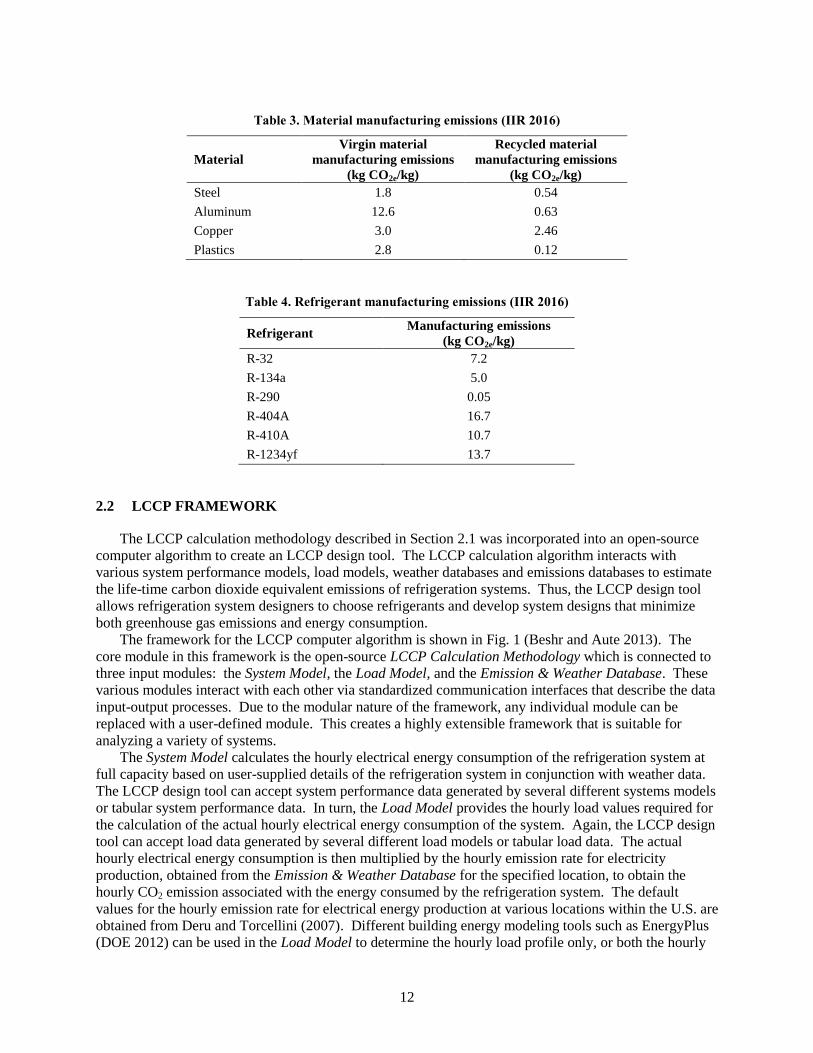
Table 3 shows the emission factors associated with the manufacture of 100% virgin and 100%
recycled materials that are used in refrigeration systems. Since many materials used today are a mixture
of virgin and recycled materials, the actual emission factor associated with manufacturing these materials
would lie somewhere between the virgin and recycled values listed in Table 3. Table 4 lists the emission
factors for the manufacture of several refrigerants. The values reported in Table 4 are an average of data
obtained from various manufactures (IIR 2016).
12
Table 3. Material manufacturing emissions (IIR 2016)
Material
Virgin material
manufacturing emissions
(kg CO2e/kg)
Recycled material
manufacturing emissions
(kg CO2e/kg)
Steel 1.8 0.54
Aluminum 12.6 0.63
Copper 3.0 2.46
Plastics 2.8 0.12
Table 4. Refrigerant manufacturing emissions (IIR 2016)
Refrigerant Manufacturing emissions
(kg CO2e/kg)
R-32 7.2
R-134a 5.0
R-290 0.05
R-404A 16.7
R-410A 10.7
R-1234yf 13.7
2.2 LCCP FRAMEWORK
The LCCP calculation methodology described in Section 2.1 was incorporated into an open-source
computer algorithm to create an LCCP design tool. The LCCP calculation algorithm interacts with
various system performance models, load models, weather databases and emissions databases to estimate
the life-time carbon dioxide equivalent emissions of refrigeration systems. Thus, the LCCP design tool
allows refrigeration system designers to choose refrigerants and develop system designs that minimize
both greenhouse gas emissions and energy consumption.
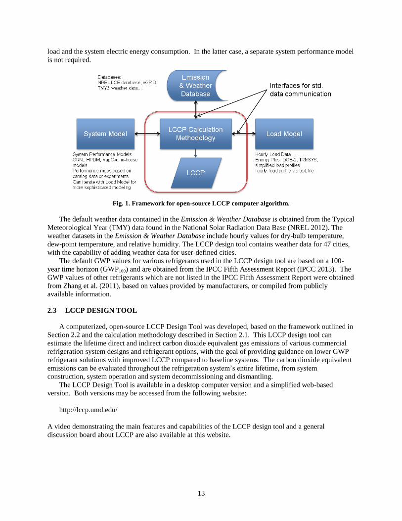
The framework for the LCCP computer algorithm is shown in Fig. 1 (Beshr and Aute 2013). The
core module in this framework is the open-source LCCP Calculation Methodology which is connected to
three input modules: the System Model, the Load Model, and the Emission & Weather Database. These
various modules interact with each other via standardized communication interfaces that describe the data
input-output processes. Due to the modular nature of the framework, any individual module can be
replaced with a user-defined module. This creates a highly extensible framework that is suitable for
analyzing a variety of systems.
The System Model calculates the hourly electrical energy consumption of the refrigeration system at
full capacity based on user-supplied details of the refrigeration system in conjunction with weather data.
The LCCP design tool can accept system performance data generated by several different systems models
or tabular system performance data. In turn, the Load Model provides the hourly load values required for
the calculation of the actual hourly electrical energy consumption of the system. Again, the LCCP design
tool can accept load data generated by several different load models or tabular load data. The actual
hourly electrical energy consumption is then multiplied by the hourly emission rate for electricity
production, obtained from the Emission & Weather Database for the specified location, to obtain the
hourly CO2 emission associated with the energy consumed by the refrigeration system. The default
values for the hourly emission rate for electrical energy production at various locations within the U.S. are
obtained from Deru and Torcellini (2007). Different building energy modeling tools such as EnergyPlus
(DOE 2012) can be used in the Load Model to determine the hourly load profile only, or both the hourly
13
load and the system electric energy consumption. In the latter case, a separate system performance model
is not required.
Fig. 1. Framework for open-source LCCP computer algorithm.
The default weather data contained in the Emission & Weather Database is obtained from the Typical
Meteorological Year (TMY) data found in the National Solar Radiation Data Base (NREL 2012). The
weather datasets in the Emission & Weather Database include hourly values for dry-bulb temperature,
dew-point temperature, and relative humidity. The LCCP design tool contains weather data for 47 cities,
with the capability of adding weather data for user-defined cities.
The default GWP values for various refrigerants used in the LCCP design tool are based on a 100-
year time horizon (GWP100) and are obtained from the IPCC Fifth Assessment Report (IPCC 2013). The
GWP values of other refrigerants which are not listed in the IPCC Fifth Assessment Report were obtained
from Zhang et al. (2011), based on values provided by manufacturers, or compiled from publicly
available information.
2.3 LCCP DESIGN TOOL
A computerized, open-source LCCP Design Tool was developed, based on the framework outlined in
Section 2.2 and the calculation methodology described in Section 2.1. This LCCP design tool can
estimate the lifetime direct and indirect carbon dioxide equivalent gas emissions of various commercial
refrigeration system designs and refrigerant options, with the goal of providing guidance on lower GWP
refrigerant solutions with improved LCCP compared to baseline systems. The carbon dioxide equivalent
emissions can be evaluated throughout the refrigeration system’s entire lifetime, from system
construction, system operation and system decommissioning and dismantling.
The LCCP Design Tool is available in a desktop computer version and a simplified web-based
version. Both versions may be accessed from the following website:
http://lccp.umd.edu/
A video demonstrating the main features and capabilities of the LCCP design tool and a general
discussion board about LCCP are also available at this website.

14
2.3.1 Desktop LCCP Design Tool
The main window of the Desktop LCCP Design Tool is shown in Fig. 2. From this window, users
can input detailed information regarding the particular application and specify how the energy simulation
and load modeling will be performed. Once all the required input data is entered, the LCCP analysis can
be initiated and the results can be viewed from the main window.
Fig. 2. Desktop LCCP Design Tool main input window.
In the Application Information window, shown in Fig. 3, details of the refrigeration or heat pump
system to be modeled are specified. System types which can be modeled include centralized direct
expansion (DX) supermarket refrigeration systems, secondary loop supermarket refrigeration systems,
air-source heat pumps, and water chillers. The total refrigerant charge, annual refrigerant leakage rate,
and mass of the system are also specified in the Application Information window. In addition, the
location of the system is specified and the operating lifetime of the system is specified. Based on the
location, the corresponding weather data and emissions values will be obtained from the TMY data files.
Finally, default values for refrigerant GWP and CO2e emissions associated with the production of various
materials are provided, and the user may adjust these values as necessary.

15
Fig. 3. Application Information input window.
In the Simulation Information window, shown in Fig. 4, the user specifies the path to the energy
simulation tool executable file which is to be used to calculate the annual energy consumption of the
refrigeration or heat pump system. The user also provides the command line prompt which is used to
initiate the simulation software executable along with any required input arguments. Energy models
which can be used include publically available models such as EnergyPlus or proprietary models
developed by the user.

16
Fig. 4. Simulation Information input window.
In the Load Information input window, shown in Fig. 5, the user specifies the hourly annual load
profile that the refrigeration or heat pump system is subjected to. The load profile is then used in
conjunction with the energy simulation tool to determine the hourly energy consumption of the
refrigeration or heat pump system.
The Desktop LCCP Design Tool contains a built-in load profile which is suitable for commercial
refrigeration applications. Alternatively, the user may specify the load profile via a user-supplied text
file. This text file should be in a comma separated value format (.csv) with the first column containing
the hours of the day and the second column containing the corresponding load values. Finally, the load
profile may be determined using EnergyPlus. For this method, the user specifies the paths to the files
required to execute EnergyPlus. When selecting this option, EnergyPlus can be used to obtain only the
hourly load values (and then a separate system simulation software is used to calculate the system’s
hourly energy consumption) or EnergyPlus can be used to obtain both the hourly load and the system’s
hourly power consumption (without using a separate energy system simulation software).
Fig. 5. Load Information input window.
After all of the required input data has been entered into the Application Information, Simulation
Information and Load Information windows, the user initiates the LCCP calculation by pressing the green
arrow button found on the main window of the LCCP Design Tool. After the calculations are complete,

17
the results may be viewed by pressing the Results tab found on the main window of the LCCP Design
tool.
A sample Results window is shown in Fig. 6. Details of the direct and indirect emissions are
provided in tabular form, and the results are also summarized graphically in the form of pie charts. The
graphical summary may be copied and pasted into word processing or presentation documents.
Fig. 6. Desktop LCCP Design Tool results window.
Finally, the Desktop LCCP Design Tool allows users to perform sensitivity analyses and uncertainty
analyses. A sensitivity analysis can be used to determine the effect that a change in one or more of the
input variables has on the resulting total CO2e emissions of the system. Furthermore, since many of the
input variables used in the LCCP analysis are not know precisely, an analysis can be performed in which
the uncertainty of each of the various input parameters can be specified, and a bound on the resulting total
CO2e emissions of the system can be determined.
2.3.2 Web-based LCCP Design Tool
While the desktop version of the LCCP design tool allows for the detailed analysis of any HVAC&R
system type, the web-based LCCP design tool allows users to more easily determine the lifetime carbon
dioxide equivalent emissions from a few pre-selected system types, such as supermarket refrigeration
systems and residential heat pump systems. The input screen of the web-based LCCP Design Tool is
shown in Fig. 7 for a medium-temperature direct expansion (DX) refrigeration system for supermarket
applications. From this screen, users can input detailed information regarding the refrigeration system to
be modeled, including the following:
System location
System lifetime
Type of refrigerant and refrigerant charge
Annual refrigerant leak rate and refrigerant service leakage rate

18
Degree of subcooling at the expansion device
Degree of superheat at the evaporator outlet
Nominal load
Compressor efficiency and compressor displacement
Condenser and evaporator tube diameter and length
Air-side and refrigerant-side heat transfer coefficients
The results of the LCCP analysis are displayed in the output screen, an example of which is shown in
Fig. 8. Summary plots show the breakdown of direct and indirect emissions as well as the components
which make up the direct and indirect emissions. The detailed emissions data is also present in tabular
form.
Fig. 7. Web-based LCCP Design Tool data input screen.
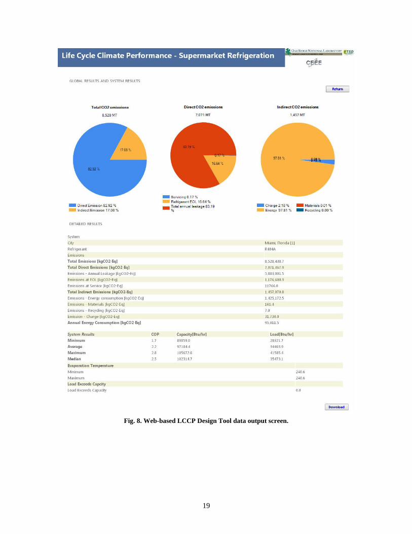
19
Fig. 8. Web-based LCCP Design Tool data output screen.

20

21
3. LCCP ANALYSIS OF REFRIGERATION SYSTEMS
The LCCP Design Tool described in Chapter 2 was used to determine the life-time carbon dioxide
equivalent emissions from a variety of supermarket refrigeration system types using a variety of
refrigerant options. The LCCP analyses are presented in several publications (Abdelaziz, Fricke, and
Vineyard 2012; Fricke, Abdelaziz, and Vineyard 2013; Beshr, Aute, Fricke, et al. 2014; Beshr, Aute,
Abdelaziz, et al. 2014; Beshr, Aute, Sharma, et al. 2014; Beshr et al. 2015). A summary of these analyses
is provided in this section.
Because supermarket refrigeration systems typically have significant refrigerant charge leakage and
high electricity consumption, they generate considerable direct and indirect greenhouse gas emissions. A
typical 35,000 ft2 (3300 m
2) grocery store can consume two to three million kilowatt-hours of energy
which results in significant indirect CO2e emissions. In addition, a typical supermarket with the
traditional multiplex direct expansion (DX) refrigeration system requires approximately 3000 to 5000 lb
(1400 to 2300 kg) of refrigerant, and the refrigeration system can have an average annual refrigerant
charge loss of 30% (Faramarzi and Walker 2004). High or moderate GWP refrigerants in conjunction
with these high refrigerant leak rates contributes to significant direct CO2e emissions. Methods for
reducing the negative environmental impact of commercial refrigeration systems include using low or
zero GWP refrigerants, improving the energy efficiency of the refrigeration systems, and designing
refrigeration systems with one of the primary performance criterion being to minimize the environmental
impact.
Many efforts are underway to develop suitable low GWP alternative refrigerants for use in
commercial refrigeration. The synthetic alternative refrigerants proposed thus far are mostly blends
comprised of R-32, R-1234yf and/or R-1234ze(E), along with other HFC refrigerants, in an effort to
obtain a balance between low GWP, affordability, safety, and system efficiency. One of the promising
refrigerants for commercial systems is the zeotropic blend R-448A, which shows competitive
performance with, and much lower GWP than, R-404A (Yana Motta and Spatz 2012).
The open-source LCCP Design Tool discussed in Chapter 2 was used to compare the LCCP of four
commercial refrigeration system configurations, using four refrigerants (R-404A, R-448A, R-744 [CO2],
and L-40), in six US cities representing different climate zones. The four refrigeration systems include
the multiplex direct expansion (DX) system, the cascade/secondary loop system, the transcritical CO2
booster system, and the medium-temperature secondary loop/low-temperature DX system. Finally, a
sensitivity analysis was performed to identify the relative importance of various input parameters on the
calculated total CO2e emissions of supermarket refrigeration systems.
3.1 ENERGY MODELING
To determine the emissions associated with the energy consumption of the refrigeration systems over
their lifetimes, EnergyPlus (DOE 2012) was used to model a typical supermarket in relevant U.S.
locations to incorporate the climate significance. EnergyPlus simulations provide estimates of the hourly
electric energy consumption of the commercial refrigeration systems. The resulting hourly electric
consumption was then multiplied by the hourly electric emission rate for the relevant interconnect region
based on data published by Deru and Torcellini (2007). The annual emissions were then multiplied by the
system lifetime to estimate the total indirect emissions.
The EnergyPlus supermarket model used in this study was based on the new construction reference
supermarket model developed by the U.S. Department of Energy (Deru et al. 2011). This single-story
supermarket model has a floor area of 45,000 ft2 (4,181 m
2) with a floor-to-ceiling height of 20 ft (6.1 m),
and is divided into six zones (office, dry storage, deli, sales, produce and bakery), as shown in Fig. 9.
Exterior wall construction consists of stucco, concrete block, insulation and gypsum while roof
construction consists of roofing membrane, insulation and metal decking. Internal loads include people
and lighting, as well as miscellaneous gas and electric loads in the deli and bakery zones. Heating and

22
air-conditioning are provided by packaged constant volume units with gas heat and electric cooling.
Specifications for the refrigerated display cases and walk-in coolers/freezers used in the model
supermarket are shown in Tables 5 and 6, respectively. These tables report the size, cooling capacity,
power input (for evaporator fans, lighting, defrost heaters and anti-sweat heaters) and operating
temperature of the display cases and walk-ins, based on representative manufacturers’ information.
Fig. 9. EnergyPlus supermarket model.
Table 5. Refrigerated display case specifications used in supermarket energy modeling (Beshr et al. 2015)
Case Type Length, ft
(m)
Cooling
Capacity,
Btu/(h·ft)
(W/m)
Evaporator
Fan, W/ft
(W/m)
Lighting,
W/ft
(W/m)
Defrost,
W/ft (W/m)
Anti-
Sweat
Heater,
W/ft
(W/m)
Case
Temperature,
°F (°C)
Medium-Temperature
Multi-deck
meat
120
(36.6)
1500
(1442)
27
(88)
12
(39)
135
(443)
20
(66)
36
(2.2)
Multi-deck
other
260
(79.2)
1500
(1442)
12
(41)
18
(60) 0 0
36
(2.2)
Low-Temperature
Reach-in 268
(81.7)
560
(538)
20
(66)
33
(108)
400
(1312)
71
(233)
5.0
(-15.0)
Single-level
open
128
(39.0)
550
(529)
10
(33) 0
420
(1378)
24
(79)
10
(-12.0)

23
Table 6. Refrigerated walk-in cooler/freezer specifications used in supermarket energy modeling
(Beshr et al. 2015)
Walk-In Type Area, ft
2
(m2)
Cooling
Capacity,
Btu/(h·ft2)
(W/m2)
Evaporator
Fan, W/ft2
(W/m2)
Lighting,
W/ft2
(W/m2)
Defrost,
W/ft2
(W/m2)
Anti-
Sweat
Heater,
W/ft2
(W/m2)
Walk-In
Temperature,
°F (°C)
Medium-Temperature
Meat Cooler 400
(37.2)
60
(190)
4
(40)
1
(11)
20
(210) 0
36
(2.2)
Food Cooler 2600
(241.5)
60
(190)
2
(26)
1
(11) 0 0
36
(2.2)
Low-Temperature
Food Freezer 1000
(92.9)
79
(250)
4
(43)
1
(11)
29
(310) 0
-10
(-23.3)
To determine the significance of climate on refrigeration system performance, the energy
consumption of the model supermarket was estimated for six U.S. cities using EnergyPlus. These six
cities, shown in Table 7, are representative of several of the climate zones in the U.S. (Baechler et al.
2010).
Table 7. Climate zones and cities used in the LCCP analysis
Climate Zone City
Annual Average
Temperature, °F
(°C)
Average Hourly Emission Rate for
Electricity Production, lb CO2/kWh
(kg CO2/kWh)
1A Miami, FL 76.8
(24.9)
1.49
(0.678)
2B Phoenix, AZ 74.8
(23.8)
1.67
(0.757)
3B Los Angeles, CA 63.1
(17.3)
0.77
(0.351)
4B Albuquerque, NM 57.6
(14.2)
2.43
(1.10)
5A Chicago, IL 50.0
(10.0)
1.41
(0.638)
8 Fairbanks, AK 28.2
(-2.1)
1.71
(0.774)
3.2 REFRIGERATION SYSTEMS
In this study, four different commercial refrigeration system designs were investigated that serve the
medium-temperature and low-temperature loads of the model supermarket described in Section 3.1.
3.2.1 Multiplex Direct Expansion (DX) System (S1)
The first refrigeration system (designated as S1) is the typical multiplex direct expansion (DX)
supermarket refrigeration system, as shown in Fig. 10. This refrigeration system consists of a combined

24
medium-temperature (MT) and low-temperature (LT) direct expansion (DX) compressor rack with
mechanical subcooling and an air-cooled condenser. Two such systems are used to satisfy the
refrigeration loads of the model supermarket, and the refrigeration load and refrigerant charge for each
system is summarized in Table 8. The compressors used for the two racks were modeled based on
commercially available compressors with published performance maps.
In this study, the multiplex DX system using R-404A as the refrigerant is considered to be the
baseline for comparison. The alternative refrigerant, R-448A, was also considered for use in this system,
since R-448A has a GWP which is nearly two-thirds less than that of R-404A, and it is designed to be a
near drop-in replacement for R-404A.
Fig. 10. Multiplex direct expansion (DX) refrigeration system (System S1).
Table 8. Multiplex DX refrigeration system configuration (System S1)
(Beshr et al. 2015)
Compressor rack MT capacity,
Btu/h (kW)
LT capacity,
Btu/h (kW)
Refrigerant
charge, lb (kg)†
1 570 000
(167.1)
220 000
(64.6)
5050
(2290)
2 180 000
(52.8)
80 000
(23.4)
1650
(750)
† Charge values are estimated, based on data provided by PG&E (2011).
3.2.2 Cascade/Secondary Loop System (S2) using R-448A and CO2
The second system (designated as S2) considered in this study was a cascade/secondary loop system,
shown in Fig. 11, in which R-448A refrigerant is used in the high-temperature circuit of the cascade
system and R-744 is used as the refrigerant in the low-temperature circuit of the cascade system. The LT
loads are served by direct expansion of R-744 in the low-temperature circuit while the MT loads are
served by a pumped liquid R-744 secondary loop, which is chilled by the R-448A circuit. In this study,

25
two air-cooled cascade/secondary loop systems were modeled to satisfy the loads of the model
supermarket, and the refrigeration load and refrigerant charge for each system are summarized in Table 9.
Compressor maps for commercially available HFC and R-744 compressors were used for the energy
simulations.
Fig. 11. Cascade/secondary loop system (System S2) using R-448A and CO2.
Table 9. Cascade/secondary loop system (System S2) using R-448A and R-744
(Beshr et al. 2015)
Compressor rack MT capacity,
Btu/h (kW)
LT capacity,
Btu/h (kW) Refrigerant charge, lb (kg)
1 405 000
(118.6)
220 000
(64.6)
HFC: 2170 (985)
R-744: 1150 (520)
2 345 000
(101.2)
80 000
(23.4)
HFC: 1850 (840)
R-744: 420 (190)
3.2.3 Transcritical R-744 (CO2) Booster System (S3)
The third system (designated as S3) considered in this study was the transcritical R-744 (CO2) booster
configuration, as shown in Fig. 12, where both the MT and LT loads are served by direct expansion of
CO2. The heat rejection from the system occurs either supercritically or subcritically, depending upon the
outdoor ambient temperature, through an air-cooled gas cooler. Two such systems are used to satisfy the
refrigeration loads of the model supermarket, and the refrigeration load and refrigerant charge for each
system are summarized in Table 10.
When the compressor discharge conditions are such that the R-744 is in the supercritical region, then
the high-side operating pressure is independent of the gas cooler exit temperature (Sawalha 2008). For a

26
given gas cooler exit temperature, there is an optimum pressure to achieve the maximum coefficient of
performance (COP) (Ge and Tassou 2011). Several researchers have developed correlations to determine
the optimum high-side pressure in transcritical R-744 refrigeration systems, and in the energy simulations
performed in this study, the optimal gas pressure control based on the correlation of Ge and Tassou
(2011) was used.
Fig. 12. Transcritical R-744 (CO2) booster refrigeration system (System S3).
Table 10. Transcritical R-744 (CO2) booster refrigeration
system configuration (System S3) (Beshr et al. 2015)
Compressor rack MT capacity,
Btu/h (kW)
LT capacity,
Btu/h (kW)
Refrigerant
charge, lb (kg)
1 405 000
(118.6)
220 000
(64.6)
2000
(905)
2 345 000
(101.2)
80 000
(23.4)
1360
(615)

27
3.2.4 Secondary (MT) / Central DX (LT) System (S4)
As shown in Fig. 13, the fourth system (designated as S4) consists of two individual refrigeration
systems: (1) a secondary loop system for cooling the medium-temperature loads, and (2) a direct
expansion system for cooling the low-temperature loads. The MT loads are served by a secondary circuit
which uses propylene glycol cooled by a DX system using L-40 refrigerant (a low-GWP A2L alternative
for R-404A). The LT loads are satisfied with a separate centralized DX system utilizing R-448A
refrigerant. The refrigeration load and refrigerant charge for each of the four compressor racks which
serve the loads of the model supermarket are given in Table 11.
Fig. 13. Secondary (MT) / central DX (LT) refrigeration system (System S4).
Table 11. Secondary (MT) / central DX (LT) refrigeration system
configuration (System S4) (Beshr et al. 2015)
Compressor rack Refrigeration capacity,
Btu/h (kW)
Refrigerant Charge, lb
(kg)
MT1 570 000
(167.1)
460
(209)
MT2 180 000
(52.8)
150
(66)
LT1 220 000
(64.6)
640
(290)
LT2 80 000
(23.4)
230
(104)
3.2.5 Refrigeration System Modeling Assumptions
The saturated evaporating temperatures for the four refrigeration system types are shown in Table 12.
It was assumed that the saturated evaporating temperatures of the CO2-based refrigeration systems were
2.0°F (1.1°C) higher than that of the HFC-based systems due to the enhanced transport properties of
carbon dioxide.

28
Table 12. Evaporating temperatures for the three refrigeration systems
System Compressor rack Temperature level Saturated evaporating
temperature, °F (°C)
S1
1 MT 27.0 (-2.80)
LT -4.0 (-20.0)
2 MT 27.0 (-2.80)
LT -19.0 (-28.3)
S2
1 MT 29.0 (-1.70)
LT 0.0 (-18.0)
2 MT 29.0 (-1.70)
LT -17.0 (-27.2)
S3
1 MT 29.0 (-1.70)
LT 0.0 (-18.0)
2 MT 29.0 (-1.70)
LT -17.0 (-27.2)
S4
MT1 MT 27.0 (-2.80)
LT1 LT -4.0 (-20.0)
MT2 MT 27.0 (-2.80)
LT2 LT -19.0 (-28.3)
Additional modeling assumptions for the refrigeration systems are as follows:
For systems S1, S2 and S4, the suction line pressure drop was assumed to be 2.5 psi (17 kPa)
while the discharge line pressure drop was assumed to be 1.2 psi (8.5 kPa). The suction gas
temperature at the compressor inlet was assumed to be the saturated evaporating temperature plus
the display case superheat. The display case superheat was assumed to be 7.2°R (4.0 K) for
systems S1, S2 and S4 and 18°R (10 K) for system S3.
System S1 contains a subcooler for each LT compressor rack. The temperature of the liquid
refrigerant exiting the subcooler was set to 50°F (10°C). No subcoolers were used in systems S2
and S4. System S3 contains a liquid-suction heat exchanger just after the gas cooler. The
effectiveness of this heat exchanger was assumed to be 0.4.
The difference between the saturated condensing temperature and the ambient air for systems S1,
S2 and S4 were approximately 7.2°R (4.0 K) for ambient temperatures greater than or equal to
68°F (20°C). In addition, the minimum condensing temperature for Systems S1, S2 and S4 was
set at 72°F (22°C). No subcooling was assumed at the exit of the condensers.
For system S3, it was assumed that the temperature difference between the gas cooler outlet and
the ambient air was 5.4°R (3 K) for transcritical operation and 18°R (10 K) for subcritical
operation. During subcritical operation, the minimum condensing temperature for System S3 was
set at 50°F (10°C).
For all systems, the performance of the compressors was determined from manufacturers’
compressor maps. Inefficiencies occurring during part load operation were ignored. The
performance of the R-448A compressors was based on R-404A compressor performance by
assuming that R-448A capacity was 100% of R-404A capacity and R-448A power was 93% of
R-404A power.
The composition and global warming potential of the refrigerants used in the energy modeling and
LCCP analysis are shown in Table 13.

29
Table 13. Refrigerant composition and GWP values (ASHRAE 2016; IPCC 2013)
Refrigerant Composition (Mass %)
ASHRAE
Safety
Classification
GWP
R-744 (CO2) R-744 (100.0) A1 1
R-448A R-32/125/1234yf/134a/1234ze(E)
(26.0/26.0/20.0/21.0/7.0) A1 1273
L-40 R-32/152a/1234yf/1234ze(E) (40.0/10.0/20.0/30.0) A2L 285
R-404A R-125/143a/134a (44.0/52.0/4.0) A1 3943
Finally, the refrigeration system lifetime was assumed to be 20 years with a service interval of two
years. The annual leakage rate, refrigerant loss at end-of-life, service leakage rate, and reused refrigerant
were assumed to be 10%, 10%, 5%, and 85%, respectively (Abdelaziz, Fricke, and Vineyard 2012).
3.3 RESULTS AND DISCUSSION
The energy consumption as well as the direct, indirect and total CO2e emissions for the four
refrigeration systems operating in each of the six cities listed in Table 7 were determined. In addition, the
effect of various input parameters on the calculated CO2e emissions was determined. These results of
these analyses are presented below.
3.3.1 LCCP Analysis
The direct emissions of the four refrigeration systems (S1, S2, S3 and S4) are shown in Fig. 14. The
direct emissions are dependent on the GWP of the system refrigerant and the refrigerant charge mass.
Direct emissions are not affected by the location of the refrigeration system. It can be seen that the
transcritical CO2 booster system (system S3) has the lowest direct emissions due to the very low GWP of
its refrigerant and its low refrigerant charge mass. Although system S4 has slightly lower refrigerant
charge mass than system S3, it has higher direct emissions than S3 because S4 utilizes a refrigerant with a
much higher GWP. The baseline system, S1 with R-404A, has the highest direct emissions since it has
the largest refrigerant charge using and the highest GWP refrigerant of the four systems investigated. For
system S1, it can be seen that replacing R-404A with R-448A can reduce the direct emissions of the
system by over 67%.

30
Fig. 14. Total direct emissions from the four refrigeration systems.
The annual energy consumption and total indirect emissions associated with the four refrigeration
systems, located in the six cities listed in Table 7, are shown in Fig. 15. It was assumed that the location
of the refrigeration system does not affect its direct emissions; however, it can be seen that location does
dramatically affect the indirect emissions of the system. The energy consumption of a refrigeration
system is dependent upon the weather conditions, while the indirect emissions are dependent upon both
the refrigeration system energy consumption and the CO2 emission rate for electricity production. As
shown in Fig. 15, it can be seen that in general, the annual energy consumption of the refrigeration
systems decreases from warm to cold climates. In addition, in cold climates such as Fairbanks, the energy
consumption of the transcritical CO2 booster system (system S3) is much closer to that of the other
systems than in warmer climates such as Miami. This is because system S3 does not perform as
efficiently in warm climates as it does in cold climates. Thus, in warmer climates, system S3 tends to
have higher indirect emissions as compared to the other systems. Also, it is worth noting that the indirect
emissions in Los Angeles are much lower than that in the other cities for all four refrigeration systems,
even though the annual electricity consumption of the systems in Los Angeles is relatively high. This
behavior is due to the low hourly emission rate for electricity production in Los Angeles, as shown in
Table 7. It can be seen that for all climates, the secondary (MT)/central DX (LT) refrigeration system
(system S4) tends to have the lowest electricity consumption and hence, the lowest indirect emissions. On
the other hand, for all but the coldest climates, the transcritical CO2 booster system (system S3) results in
higher electricity consumption and higher indirect emissions.
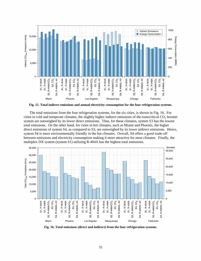
31
Fig. 15. Total indirect emissions and annual electricity consumption for the four refrigeration systems.
The total emissions from the four refrigeration systems, for the six cities, is shown in Fig. 16. For
cities in cold and temperate climates, the slightly higher indirect emissions of the transcritical CO2 booster
system are outweighed by its lower direct emissions. Thus, for these climates, system S3 has the lowest
total emissions. On the other hand, for cities in hot climates, such as Miami and Phoenix, the higher
direct emissions of system S4, as compared to S3, are outweighed by its lower indirect emissions. Hence,
system S4 is more environmentally friendly in the hot climates. Overall, S4 offers a good trade-off
between emissions and electricity consumption making it more attractive for most climates. Finally, the
multiplex DX system (system S1) utilizing R-404A has the highest total emissions.
Fig. 16. Total emissions (direct and indirect) from the four refrigeration systems.
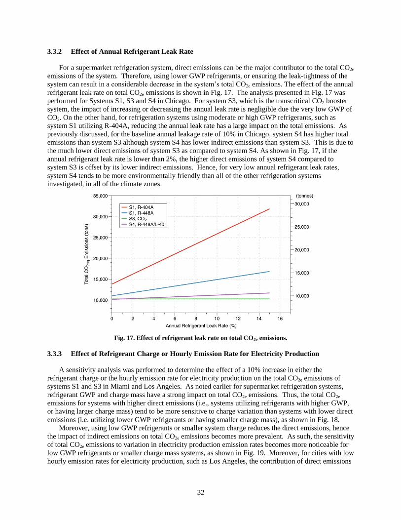
32
3.3.2 Effect of Annual Refrigerant Leak Rate
For a supermarket refrigeration system, direct emissions can be the major contributor to the total CO2e
emissions of the system. Therefore, using lower GWP refrigerants, or ensuring the leak-tightness of the
system can result in a considerable decrease in the system’s total CO2e emissions. The effect of the annual
refrigerant leak rate on total CO2e emissions is shown in Fig. 17. The analysis presented in Fig. 17 was
performed for Systems S1, S3 and S4 in Chicago. For system S3, which is the transcritical CO2 booster
system, the impact of increasing or decreasing the annual leak rate is negligible due the very low GWP of
CO2. On the other hand, for refrigeration systems using moderate or high GWP refrigerants, such as
system S1 utilizing R-404A, reducing the annual leak rate has a large impact on the total emissions. As
previously discussed, for the baseline annual leakage rate of 10% in Chicago, system S4 has higher total
emissions than system S3 although system S4 has lower indirect emissions than system S3. This is due to
the much lower direct emissions of system S3 as compared to system S4. As shown in Fig. 17, if the
annual refrigerant leak rate is lower than 2%, the higher direct emissions of system S4 compared to
system S3 is offset by its lower indirect emissions. Hence, for very low annual refrigerant leak rates,
system S4 tends to be more environmentally friendly than all of the other refrigeration systems
investigated, in all of the climate zones.
Fig. 17. Effect of refrigerant leak rate on total CO2e emissions.
3.3.3 Effect of Refrigerant Charge or Hourly Emission Rate for Electricity Production
A sensitivity analysis was performed to determine the effect of a 10% increase in either the
refrigerant charge or the hourly emission rate for electricity production on the total CO2e emissions of
systems S1 and S3 in Miami and Los Angeles. As noted earlier for supermarket refrigeration systems,
refrigerant GWP and charge mass have a strong impact on total CO2e emissions. Thus, the total CO2e
emissions for systems with higher direct emissions (i.e., systems utilizing refrigerants with higher GWP,
or having larger charge mass) tend to be more sensitive to charge variation than systems with lower direct
emissions (i.e. utilizing lower GWP refrigerants or having smaller charge mass), as shown in Fig. 18.
Moreover, using low GWP refrigerants or smaller system charge reduces the direct emissions, hence
the impact of indirect emissions on total CO2e emissions becomes more prevalent. As such, the sensitivity
of total CO2e emissions to variation in electricity production emission rates becomes more noticeable for
low GWP refrigerants or smaller charge mass systems, as shown in Fig. 19. Moreover, for cities with low
hourly emission rates for electricity production, such as Los Angeles, the contribution of direct emissions
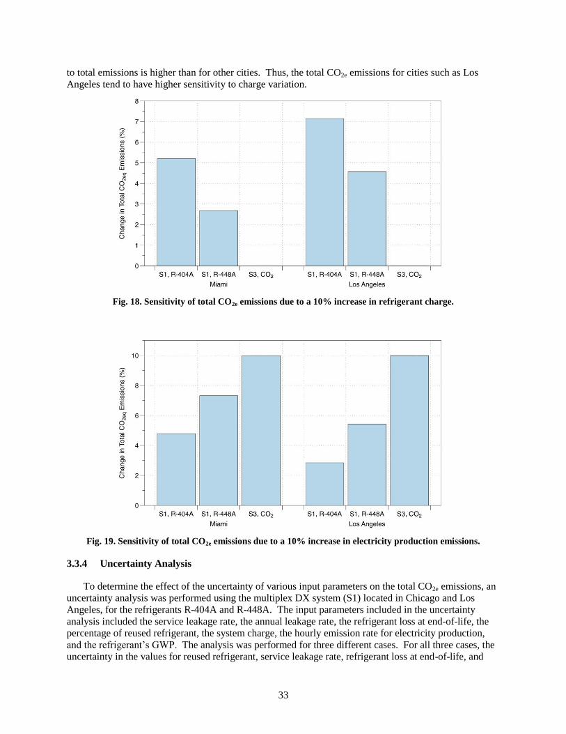
33
to total emissions is higher than for other cities. Thus, the total CO2e emissions for cities such as Los
Angeles tend to have higher sensitivity to charge variation.
Fig. 18. Sensitivity of total CO2e emissions due to a 10% increase in refrigerant charge.
Fig. 19. Sensitivity of total CO2e emissions due to a 10% increase in electricity production emissions.
3.3.4 Uncertainty Analysis
To determine the effect of the uncertainty of various input parameters on the total CO2e emissions, an
uncertainty analysis was performed using the multiplex DX system (S1) located in Chicago and Los
Angeles, for the refrigerants R-404A and R-448A. The input parameters included in the uncertainty
analysis included the service leakage rate, the annual leakage rate, the refrigerant loss at end-of-life, the
percentage of reused refrigerant, the system charge, the hourly emission rate for electricity production,
and the refrigerant’s GWP. The analysis was performed for three different cases. For all three cases, the
uncertainty in the values for reused refrigerant, service leakage rate, refrigerant loss at end-of-life, and

34
annual leakage rate were assumed to be 20%, while the refrigerant charge uncertainty was assumed to be
5%. The power plant emissions and the refrigerant GWP uncertainties were varied. For cases 1, 2, and 3,
the uncertainty in energy production emissions was 5%, 5%, and 20%, respectively, while the refrigerant
GWP uncertainty was 20%, 5%, and 5%, respectively. The range of uncertainty for these various
parameters is summarized in Table 14.
Table 14. Summary of uncertainty in LCCP parameters
Parameter Uncertainty (%)
Case 1 Case 2 Case 3
Reused refrigerant 20 20 20
Service leakage rate 20 20 20
Refrigerant loss at end-of-life 20 20 20
Annual leakage rate 20 20 20
Charge 5 5 5
Power plant emission 5 5 20
Refrigerant GWP 20 5 5
The resulting uncertainties for the total CO2e emissions of the multiplex DX system (S1), due to
uncertainties in the input parameters, are shown in Table 15. The partial derivatives of the total emissions
with respect to each of the input parameters are shown in Table 16, accompanied by the percentage
difference between the derivatives values when utilizing R-448A compared to R-404A. The partial
derivatives do not change for any of the three cases. This is because the derivatives do not depend on the
magnitude of uncertainty of the input parameters, but rather on the baseline design itself. Thus, changing
the location from Chicago to Seattle only causes a change in the partial derivative which depends on the
location, such as the derivative of the total emissions with respect to the hourly emission rate for
electricity production. Also, the results show that shifting to a low GWP refrigerant causes a noticeable
drop in the impact of the uncertainty in the input parameters related to the direct emissions (i.e., service
leakage rate, refrigerant loss at end-of-life, annual leakage rate, and system refrigerant charge) on the total
emissions. This results in a more dominant impact of the power plant emissions uncertainty on the
uncertainty of the total system emissions. Thus, for the low GWP refrigerant (R-448A) in Chicago for
case 3, the uncertainty of the system’s total emissions is higher than for R-404A. Finally, performing the
same uncertainty analysis for S3 in Los Angeles results in LCCP uncertainty of 5%, 5%, and 19.98% for
cases 1, 2, and 3, respectively. This is due to the small direct emissions of this system which makes the
uncertainty in the power plant emissions much more dominant than in the case of other systems. This
causes the uncertainty in the transcritical CO2 booster system’s LCCP to follow the value of the
uncertainty in the power plant emissions.

35
Table 15. Uncertainties in the total CO2e emissions of the multiplex DX system (S1)
Case City Refrigerant Uncertainty in total
CO2e emissions (%)
Case 1
Chicago R-404A 15.82
R-448A 9.40
Los Angeles R-404A 18.64
R-448A 12.17
Case 2
Chicago R-404A 10.69
R-448A 6.76
Los Angeles R-404A 12.52
R-448A 8.40
Case 3
Chicago R-404A 13.15
R-448A 14.47
Los Angeles R-404A 13.68
R-448A 13.45
Table 16. Partial derivatives of the total emissions with respect to each of the input parameters
Chicago Los Angeles
Parameter Partial derivative Partial derivative
R-404A R-448A
Difference,
% R-404A R-448A
Difference,
%
Reused refrigerant -2.30E+04 -1.10E+04 -52.1 -2.30E+04 -1.10E+04 -52.1
Service leakage rate 5.43E+07 1.75E+07 -67.7 5.43E+07 1.75E+07 -67.7
Refrigerant loss at
end-of-life 5.43E+06 1.75E+06 -67.7 5.43E+06 1.75E+06 -67.7
Annual leakage rate 1.09E+08 3.53E+07 -67.6 1.09E+08 3.53E+07 -67.6
Refrigerant charge 1.03E+04 3.33E+03 -67.7 1.03E+04 3.33E+03 -67.7
Power plant emission 1.45E+07 1.40E+07 -3.6 1.61E+07 1.55E+07 -3.4
Refrigerant GWP 3.58E+03 3.58E+03 0.0 3.58E+03 3.58E+03 0.0
3.4 SUMMARY
A flexible LCCP design tool was developed for the design and evaluation of supermarket
refrigeration systems. The LCCP framework is open-source and can be easily extended to the analysis of
other refrigeration and vapor compression technologies. This LCCP design tool was used to compare the
environmental impact of four different supermarket refrigeration systems in six US cities. Comparing the
total emissions for different cities suggests that the transcritical CO2 booster system has the lowest CO2
equivalent emissions, according to this analysis, in cold and temperate. Also, the R-448A/L-40 secondary
circuit refrigeration system was found to offer a good balance between emissions and electricity
consumption for hot climates. The parametric analysis showed that shifting towards low GWP
refrigerants decreases the effect of the annual leak rate on the total system emissions. Moreover, the
sensitivity analysis showed that shifting towards low GWP refrigerants, or more charge conservative
systems increases the effect of the hourly emission rate for electricity production on the total system
emissions. Finally, an uncertainty analysis was performed showing that using low GWP refrigerants, or

36
more charge conservative systems causes a noticeable drop in the impact of the uncertainty in the inputs
related to the direct emissions.

37
4. LABORATORY EVALUATION OF ALTERNATIVE REFRIGERANTS
The energy performance of an alternative lower global warming potential refrigerant was evaluated in
a laboratory-scale commercial refrigeration system, and its performance was compared to that of a
commonly used higher GWP refrigerant found in the commercial refrigeration industry. The aim is to
identify safe, energy efficient, low GWP alternatives to today’s commonly used high GWP refrigerants.
The two refrigerants investigated were R-404A and R-448A. R-404A is a commonly used refrigerant in
the commercial refrigeration industry and has a relatively high global warming potential, while R-448A is
a new lower GWP alternative for R-404A.
R-404A is a zeotropic blend of several hydrofluorocarbon (HFC) refrigerants, and consists of 44.0%
(by mass) R-125, 52.0% (by mass) R-143a and 4.0% (by mass) R-134a. The resulting mixture exhibits a
low temperature glide of less than 1.1°F (0.6°C) under typical operating conditions. The global warming
potential of R-404A is relatively high, with a value of 3,943 (IPCC 2013). R-404A has an ASHRAE
safety classification of A1, indicating that it has low toxicity and is non-flammable (ASHRAE 2016).
R-448A is a non-flammable zeotropic blend of several HFC and hydrofluoro-olefin (HFO)
refrigerants, including R-32 (26.0% by mass), R-125 (26.0% by mass), R-1234yf (20.0% by mass),
R-134a (21.0% by mass) and R-1234ze(E) (7.0% by mass). R-448A exhibits a larger temperature glide
than R-404A, with a value no more than 11°F (6°C) under typical operating conditions. The global
warming potential of R-448A is significantly lower than that of R-404A, with a value of approximately
1,273 (IPCC 2013). R-448A has an ASHRAE safety classification of A1, indicating that it has low
toxicity and is non-flammable (ASHRAE 2016).
4.1 COMMERCIAL REFRIGERATION SYSTEM DESCRIPTION
The laboratory-scale commercial refrigeration system installed in the environmental test chambers at
the Oak Ridge National Laboratory, that was used to investigate the energy performance of R-404A and
R-448A, consists of components typically found in most U.S. supermarket refrigeration systems. These
components include a compressor rack, an air-cooled condenser and several medium-temperature (MT)
and low-temperature (LT) refrigerated display cases. A schematic of the laboratory-scale refrigeration
system, showing these various components as well as several instrumentation points, is shown in Fig. 20.
Fig. 20. Schematic of laboratory-scale commercial refrigeration system.

38
The refrigeration system has a low-temperature cooling capacity of approximately 5 tons at −20°F
(18 kW at −29°C) and a medium-temperature cooling capacity of approximately 10 to 15 tons at 25°F (35
to 53 kW at −4°C). Three open vertical display cases, each 12 ft (3.7 m) in length, constitute the low-
temperature load. The medium-temperature load consists of two open vertical display cases, each 12 ft
(3.7 m) in length, as well as a “false” load provided by a plate heat exchanger and glycol loop.
The compressor rack and air-cooled condenser are installed in a temperature and humidity controlled
“outdoor” environmental chamber while the refrigerated display cases are installed in a separate
temperature and humidity controlled “indoor” environmental chamber. For both chambers, the
temperature can be controlled between 0 to 130°F (−18 to 54°C) and the humidity can be controlled
between 30 to 90%. Thus, the air-cooled condenser can be exposed to typical outdoor ambient conditions
while the refrigerated display cases operate in an environment typical of that found in the sales area of a
supermarket.
4.1.1 Compressor Rack
The compressor rack, shown in Fig. 21, consists of several refrigerant compressors and the associated
piping that forms the low-temperature and medium-temperature liquid headers and suction headers as
well as the common discharge header. The refrigeration loads (i.e., the refrigerated display cases) are
connected to the low-temperature and medium-temperature liquid and suction headers of the compressor
rack and the condenser is connected to the discharge header of the compressor rack.
Fig. 21. Compressor rack.
The compressor rack of the commercial refrigeration system is unique in that it contains two types of
compressors that are commonly found in supermarket refrigeration systems: reciprocating compressors
and scroll compressors. Note that only one type of compressor (i.e., reciprocating or scroll) is operated at
one time. In essence, the compressor rack is two racks in one: a reciprocating compressor rack and a
scroll compressor rack. Having both reciprocating and scroll compressors allows for system performance
tests to be performed using the two common compressor types employed in supermarket refrigeration
systems.
For each compressor type, the refrigeration system contains two low-temperature compressors and
two medium-temperature compressors. In addition, for each compressor type and temperature level, the
compressor rack contains a primary compressor that is variable capacity (capable of modulating its

39
capacity from 10% to 100%), and a secondary compressor that is fixed capacity. The primary compressor
is used first to satisfy the refrigeration load, and it can modulate its capacity to match the applied load. If
the primary compressor is not sufficient to satisfy the load, then the secondary compressor operates as
well, with the primary compressor modulating its capacity to match the load.
The refrigerating capacity and power requirements for both the reciprocating and scroll compressors
are given in Table 17. In addition, the total refrigerating capacity of the compressor rack is given in
Table 18.
Table 17. Compressor specifications for laboratory-scale refrigeration system
Compressor
type
Temperature
level
Capacity
control
Refrigerating
capacity, Btu/h
(kW)*
Power, kW*
Reciprocating LT Variable 32 000
(9.38) 5.70
Reciprocating LT Fixed 32 000
(9.38) 5.70
Reciprocating MT Variable 92 300
(27.1) 8.50
Reciprocating MT Fixed 92 300
(27.1) 8.50
Scroll LT Variable 32 300
(9.47) 5.20
Scroll LT Fixed 32 300
(9.47) 5.20
Scroll MT Variable 56 300
(16.5) 5.23
Scroll MT Fixed 56 300
(16.5) 5.23
*Refrigerating capacity and power are given for the following operating conditions using
R-404A:
LT: −20°F (−29°C) evaporating temperature, 105°F (41°C) condensing temperature
MT: 25°F (−3.9°C) evaporating temperature, 105°F (41°C) condensing temperature
Table 18. Compressor rack capacity for
laboratory-scale refrigeration system
Compressor
type
Temperature
level
Compressor rack
capacity, Btu/h (kW)
Reciprocating
LT 64 000
(18.8)
MT 184 600
(54.1)
Scroll
LT 64 600
(18.9)
MT 112 600
(33.0)

40
4.1.2 Refrigerated Display Cases
The three low-temperature and two medium-temperature display cases of the commercial
refrigeration system are open, vertical multi-deck models, each 12 ft (3.7 m) in length. The rated capacity
of each LT case is 18 100 Btu/h (5.30 kW) while the rated capacity of each MT case is 17 100 Btu/h
(5.01 kW), according to ASHRAE Standard 72 (2005). Fig. 22 shows representative photos of the low-
temperature and medium-temperature display cases.
(a) (b)
Fig. 22. Low-temperature (a) and medium-temperature (b) display cases.
Each low-temperature display case has one evaporator with one corresponding mechanical
thermostatic expansion valve. Each medium-temperature display case contains two evaporators, with
each evaporator having its own thermostatic expansion valve. Thus, each MT display case contains two
thermostatic expansion valves. The LT and MT display cases utilize fluorescent lighting and shaded-pole
evaporator fan motors. In addition, the LT display cases have anti-sweat heaters. Finally, the LT display
cases utilize electric defrost heaters while the MT display cases utilize off-cycle defrost. The
specifications for the low-temperature and medium-temperature display cases are shown in Table 19.
In addition to the refrigerated display cases, a medium-temperature “false” load is also incorporated
into the refrigeration system. This false load consists of a plate heat exchanger with two medium-
temperature refrigerant circuits on one side of the heat exchanger and a glycol circuit on the other side.
The false load provides an additional load of approximately 50 000 Btu/h (14.7 kW) to the medium-
temperature side of the refrigeration system.

41
Table 19. Refrigerated display case specifications
Display case parameter Low-temperature display
case
Medium-temperature
display case
Type Open, vertical multi-deck Open, vertical multi-deck
Length 12 ft
(3.7 m)
12 ft
(3.7 m)
Rated Capacity 18 100 Btu/h
(5.30 kW)
17 100 Btu/h
(5.01 kW)
Fan Amperage 7.2 A 0.56 A
Lighting Amperage 4.2 A 0.72 A
Anti-Sweat Heater Amperage 8.6 A --
Defrost Type Electric Off-cycle
Defrost Amperage 20.4 A --
4.1.3 Air-Cooled Condenser
As shown in the system schematic in Fig. 20, an air-cooled condenser is used to reject heat from the
refrigeration system. The condenser accepts the discharge refrigerant vapor from the compressor rack,
condenses the refrigerant, and discharges the condensed refrigerant into a liquid receiver. The air-cooled
condenser has four variable speed fans and its rated capacity, with R-404A, is 351 000 Btu/h (103 kW) at
a temperature difference of 10°F (5.6°C) between the saturated condensing temperature and the ambient
air. Fig. 23 shows a photo of the air-cooled condenser, mounted above the liquid receiver, as installed in
the “outdoor” environmental chamber.
Fig. 23. Air-cooled condenser (top) mounted above liquid receiver (bottom).
42
4.1.4 Refrigeration System Controls
The refrigeration system controller provides the following control:
Compressor control to maintain suction pressure setpoints for the LT and MT circuits
Condenser fan speed control to maintain condensing pressure
Display case temperature control via electronic evaporator pressure regulators
Display case defrost initiation and termination
In addition to the system controller, the refrigeration system also has electronic display case superheat
controllers, and an electronic subcooler controller. Note that since the refrigerated display cases currently
utilize mechanical thermostatic expansion valves, the superheat controllers are not required. However,
superheat controllers are provided in the system in the event that electronic expansion valves are to be
used in the display cases. Also, since the false load utilizes electronic expansion valves, electronic
superheat controllers are required for the two false load refrigerant circuits.
4.1.5 Instrumentation
The laboratory-scale commercial refrigeration system was fully instrumented to monitor its
performance. Refrigerant temperature, pressure and flow rate were measured at various locations within
the system. Compressor and display case fan/lighting and defrost heater power were measured. In
addition, display case discharge and return air temperatures were measured. Table 20 lists the
specifications of the instrumentation used to measure these various quantities.
Table 20. Instrumentation specifications
Instrument Quantity measured Range Accuracy
Differential pressure
transducer
(Kele DPW-692)
Refrigerant pressure drop
across condenser
0 to 25 psi
(0 to 172 kPa) <±0.5% full scale
Mass flow meter, coriolis
(Micro Motion CMF series)
Refrigerant mass flow rate
(receiver exit, MT liquid line,
LT liquid line, display case
liquid lines)
0 to 125 lb/min
(0 to 0.94 kg/s)
Liquid flow: ±0.10%
Gas flow: ±0.50%
Mass flow meter, positive
displacement
(Omega FPD2000)
Refrigerant mass flow rate
(display case liquid lines, MT
false load liquid lines)
0.03 to 7.0 GPM
(0.0018 to 0.44 L/s) ±0.5%
Temperature/humidity sensor
(Vaisala HMT120)
Indoor and outdoor chamber
temperature and relative
humidity
Temperature:
−40 to 176°F
(−40 to 80°C)
Relative humidity:
0 to 100% RH
Temperature:
±0.36°F for 59 to 77°F
(±0.2°C for 15 to 25°C)
Relative humidity:
(for 32 to 104°F or 0 to 40°C)
0 to 90% RH: ±1.7% RH
90% to 100% RH: ±2.5% RH
Temperature/humidity sensor
(Vaisala HMT330)
Display case discharge/return
temperature and relative
humidity
Temperature:
−40 to 176°F
(−40 to 80°C)
Relative humidity:
0 to 100% RH
Temperature:
±0.36°F at 68°F
(±0.2°C at 20°C)
Relative humidity:
(for 59 to 77°F or 15 to 25°C)
0 to 90% RH: ±1% RH
90 to 100% RH: ±1.7% RH
Type-T thermocouple
Refrigerant temperature,
product temperature, display
case discharge/return
temperature
−328 to 662°F
(−250 to 350°C)
Greater of 1.8°F (1.0°C) or
or 0.75% above 32°F (0°C)

43
Instrument Quantity measured Range Accuracy
Pressure transducer
(Wika AC-1) Refrigerant pressure
0 to 300 psig
(0 to 2.17 MPa)
0 to 500 psig
(0 to 3.55 MPa)
≤1.0% of span
Watt transducer
(Ohio Semitronics GW5)
Display case power,
compressor power
0 to 2000 W
0 to 60 000 W ±0.2% of reading
4.2 TEST PLAN
For both refrigerants (R-404A and R-448A), the performance of the laboratory-scale commercial
refrigeration system, using the reciprocating compressors, was determined at four ambient temperature
conditions: 60°F, 75°F, 95°F and 105°F (16°C, 24°C, 35°C, and 41°C). For each refrigerant, the
refrigeration system setpoints were adjusted so that one LT and one MT reciprocating compressor
operated continuously at full capacity, and the condenser fan speed was adjusted to maintain
approximately a 10°F (5.6°C) temperature differential between the saturated condensing temperature and
the condenser entering air temperature. The system setpoints and operating conditions used for each
refrigerant are shown in Table 21 for operation with reciprocating compressors. In addition, the
refrigerated display case thermostatic expansion valves were adjusted to achieve a superheat of
approximately 10°F (5.6°C) at the exit of each display case.
Table 21. Refrigeration system setpoints and operating conditions
when operating with reciprocating compressors
Variable R-404A R-448A
LT suction pressure setpoint 12 psig (184 kPa) 8 psig (156 kPa)
LT compressor capacity range 80% to 100% capacity, least
cycling
80% to 100% capacity, least
cycling
MT suction pressure setpoint 45 psig (412 kPa) 38 psig (363 kPa)
MT compressor capacity range 80% to 100% capacity, least
cycling
80% to 100% capacity, least
cycling
Condenser pressure control
setpoint 126 psig (970 kPa) 126 psig (970 kPa)
Condenser fan speed Variable Variable
LT display case EPR setting 100% (fully open) 100% (fully open)
MT display case EPR setting 100% (fully open) 100% (fully open)
False load circuit 1 EPR setting 50% 50%
False load circuit 2 EPR setting 2% 2%
Similarly, when using the scroll compressors, the performance of the laboratory-scale commercial
refrigeration system was determined at four ambient temperature conditions using both refrigerants
(R-404A and R-448A): 60°F, 75°F, 95°F and 105°F (16°C, 24°C, 35°C, and 41°C). However, the
system setpoints and operating parameters were set differently than that used for the reciprocating
compressor tests. The suction pressure setpoints were set at values typical of that found in actual
operating supermarket refrigeration systems, and the condenser fan speed was adjusted to maintain

44
approximately a 10°F (5.6°C) temperature differential between the saturated condensing temperature and
the condenser entering air temperature. The system setpoints and operating conditions used for each
refrigerant are shown in Table 22 for operation with scroll compressors. In addition, the refrigerated
display case thermostatic expansion valves were adjusted to achieve a superheat of approximately 10°F
(5.6°C) at the exit of each display case.
Table 22. Refrigeration system setpoints and operating conditions
when operating with scroll compressors
Variable R-404A R-448A
LT suction pressure setpoint 17 psig (219 kPa) 14 psig (198 kPa)
LT compressor capacity range 80% to 100% capacity, least
cycling
80% to 100% capacity, least
cycling
MT suction pressure setpoint 50 psig (446 kPa) 46 psig (419 kPa)
MT compressor capacity range 80% to 100% capacity, least
cycling
80% to 100% capacity, least
cycling
Condenser pressure control
setpoint 126 psig (970 kPa) 126 psig (970 kPa)
Condenser fan speed Variable Variable
LT display case EPR setting Automatic Automatic
MT display case EPR setting Automatic Automatic
False load circuit 1 EPR setting Automatic Automatic
False load circuit 2 EPR setting Automatic Automatic
4.2.1 Data Acquisition
After the refrigeration system achieved steady-state operation at each of the test conditions, system
performance data was collected for a 24-hour period. Measurement points were sampled and recorded
once per second, and 30-second averaged data was used for the calculation of thermodynamic properties
and performance metrics.
4.2.2 Data Analysis
From the data collected during testing, system performance characteristics, as functions of ambient
conditions, were determined, including system coefficient of performance (COP), compressor isentropic
efficiency, compressor discharge temperature and pressure, suction header operating temperature and
pressure, and display case discharge air temperature.
Using the 30-second averaged data for the 24-hour test periods (consisting of 2881 data points per
test), the thermodynamic properties at the inlet and outlet of each major system component, including
compressors, display cases, false load, and condenser, were determined using REFPROP (Lemmon,
McLinden, and Huber 2013). These properties include specific volume, specific enthalpy and specific
entropy. The average value of these thermodynamic properties, as well as the average values of
refrigerant mass flow and compressor power, were then determined for the 24-hour test period. Note that
for the refrigerated display cases, the average values of the thermodynamic properties and refrigerant
mass flow excluded those periods during which the display cases were undergoing defrost.

45
The average refrigeration load, �̇�𝑖, for each display case and false load for the 24-hour test period was
calculated as follows:
�̇�𝑖 = �̇�𝑖(ℎ𝑖,𝑜𝑢𝑡 − ℎ𝑖,𝑖𝑛) (7)
where �̇�𝑖 is the average refrigerant mass flow through load i, ℎ𝑖,𝑜𝑢𝑡 is the average refrigerant enthalpy at
the exit of load i, and ℎ𝑖,𝑖𝑛 is the average refrigerant enthalpy at the inlet of load i. The average total
refrigeration load for the refrigeration system during the 24-hour test period then becomes:
�̇�𝑡𝑜𝑡𝑎𝑙 = ∑ �̇�𝑖
𝑛
𝑖=1
(8)
where n is the number of independent loads connected to the refrigeration system. Note that performance
data collected during defrost periods was ignored in the calculation of refrigeration load.
The average total compressor power, �̇�𝑡𝑜𝑡𝑎𝑙, for the 24-hour test period was determined as follows:
�̇�𝑡𝑜𝑡𝑎𝑙 = ∑ �̇�𝑖,𝐿𝑇 + ∑ �̇�𝑗,𝑀𝑇
𝑚
𝑗=1
𝑛
𝑖=1
(9)
where �̇�𝑖,𝐿𝑇 is the average input power to low-temperature compressor i, �̇�𝑗,𝑀𝑇 is the average input
power to medium-temperature compressor j, and n and m are the number of low- and medium-
temperature compressors, respectively.
The system COP was then determined from the average total refrigeration load and the average total
compressor power for the 24-hour test period:
𝐶𝑂𝑃 =�̇�𝑡𝑜𝑡𝑎𝑙
�̇�𝑡𝑜𝑡𝑎𝑙
(10)
The average uncertainty in the calculated COP values was estimated to be ±0.016 (Taylor and Kuyatt
1994).
The average isentropic efficiency of the ith compressor, 𝜂𝑖,𝑡ℎ, for the 24-hour test period was
calculated as follows:
𝜂𝑖,𝑡ℎ =�̇�𝑖(ℎ𝑐,𝑜𝑢𝑡,𝑠 − ℎ𝑐,𝑖𝑛)
�̇�𝑖,𝑎
(11)
where �̇�𝑖 is the average refrigerant mass flow rate through compressor i, ℎ𝑐,𝑜𝑢𝑡,𝑠 is the average
compressor outlet enthalpy assuming isentropic compression between the inlet and outlet pressures, ℎ𝑐,𝑖𝑛
is the average compressor inlet enthalpy determined from measured refrigerant temperature and pressure
and �̇�𝑖,𝑎 is the average measured power for compressor i. The average uncertainty in the calculated
isentropic efficiency values was estimated to be ±0.036 (Taylor and Kuyatt 1994).
4.3 RESULTS
4.3.1 Performance with Reciprocating Compressors
The total refrigerating capacity of the system, operating with reciprocating compressors using either
R-448A or R-404A, is shown in Fig. 24. It can be seen that system capacity decreases as the ambient
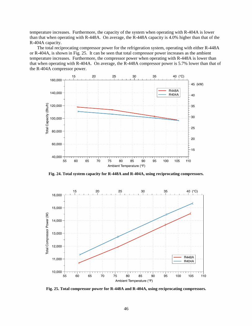
46
temperature increases. Furthermore, the capacity of the system when operating with R-404A is lower
than that when operating with R-448A. On average, the R-448A capacity is 4.0% higher than that of the
R-404A capacity.
The total reciprocating compressor power for the refrigeration system, operating with either R-448A
or R-404A, is shown in Fig. 25. It can be seen that total compressor power increases as the ambient
temperature increases. Furthermore, the compressor power when operating with R-448A is lower than
that when operating with R-404A. On average, the R-448A compressor power is 5.7% lower than that of
the R-404A compressor power.
Fig. 24. Total system capacity for R-448A and R-404A, using reciprocating compressors.
Fig. 25. Total compressor power for R-448A and R-404A, using reciprocating compressors.

47
The COP of the commercial refrigeration system, operating with either R-448A or R-404A, is shown
in Fig. 26. As noted above, the capacity of R-448A is slightly higher than that of R-404A and the
compressor power associated with R-448A is lower than that of R-404A. Overall then, the COP of the
system operating with R-448A was greater than that when operating with R-404A. The maximum
deviation between the R-448A COP and the R-404A COP was 13%. On average, the COP of the
refrigeration system operating with R-448A was 10% higher than that when operating with R-404A.
Fig. 26. Refrigeration system COP for R-448A and R-404A, using reciprocating compressors.
The total refrigerant mass flow rate for the commercial refrigeration system, operating with either
R-448A or R-404A, is shown in Fig. 27. It can be seen that as the ambient temperature increases, the
total refrigerant mass flow rate increases. On average, the total refrigerant mass flow rate of the system
operating with R-448A was found to be approximately 25% lower than that when operating with R-404A.
Fig. 27. Total refrigerant mass flow for R-448A and R-404A, using reciprocating compressors.

48
The low-temperature and medium-temperature compressor isentropic efficiencies for R-448A and
R-404A are shown in Fig. 28, for the system operating with reciprocating compressors. It can be seen
that as the ambient temperature increases, the isentropic efficiency of the compressors increases. In
addition, it can be seen that the isentropic efficiency of the compressors when operating with R-448A is
less than that when operating with R-404A. The isentropic efficiency of the low-temperature
compressors, when operating with R-448A, is on average 3.9% lower than that when operating with
R-404A. Similarly, the isentropic efficiency of the medium-temperature compressors, when operating
with R-448A, is on average 4.2% lower than that when operating with R-404A.
Fig. 28. Low-temperature (LT) and medium-temperature (MT) compressor isentropic efficiencies for
R-448A and R-404A, using reciprocating compressors.
The low-temperature and medium-temperature compressor discharge temperatures, when operating
with either R-448A or R-404A, are shown in Fig. 29. It can be seen that the compressor discharge
temperature increases as ambient temperature increases. In general, the compressor discharge
temperature of R-448A is between 16°F to 20°F (8.9°C to 11°C) greater than that of R-404A.

49
Fig. 29. Low-temperature (LT) and medium-temperature (MT) compressor discharge temperatures for
R-448A and R-404A, using reciprocating compressors.
The low-temperature and medium-temperature suction header pressures for the refrigeration system,
when operating with either R-448A or R-404A, are shown in Fig. 30, for the system operating with
reciprocating compressors. It can be seen that the suction header pressure increases slightly as the
ambient temperature increases. On average, the low-temperature suction header pressure is 2.5 psi
(17 kPa) lower with R-448A as compared to R-404A, while the medium-temperature suction header
pressure is 7.5 psi (51 kPa) lower with R-448A as compared to R-404A.
Fig. 30. Low-temperature (LT) and medium-temperature (MT) suction header pressures for R-448A and
R-404A, using reciprocating compressors.

50
Finally, Fig. 31 shows the average low-temperature and medium-temperature display case discharge
air temperatures for the commercial refrigeration system operating with either R-448A or R-404A, using
reciprocating compressors. It can be seen that the display case discharge air temperature increases
slightly as ambient temperature increases. In addition, the display case discharge air temperatures for
R-448A are lower than those for R-404A. On average, the low-temperature display case discharge air
temperature was 1.8°F (1.0°C) lower for R-448A as compared to R-404A, while the discharge air
temperature for the medium-temperature display cases was 4.4°F (2.4°C) lower when operating with
R-448A versus R-404A.
Fig. 31. Low-temperature (LT) and medium-temperature (MT) display case discharge air temperatures
for R-448A and R-404A, using reciprocating compressors.
4.3.2 Summary of Results with Reciprocating Compressors
From the data presented above, it can be seen that R-448A and R-404A performed similarly in the
laboratory-scale commercial refrigeration system while operating with the reciprocating compressors.
Compared to R-404A, R-448A exhibited an energy benefit since system COP was increased and
compressor power was decreased. On average, the efficiency of the system increased by 10% when
operating with R-448A as compared to R-404A. The refrigeration capacity of R-448A was found to be
slightly higher than that of R-404A. For the same saturated evaporating and condensing temperatures,
compressor suction pressures of R-448A were lower than that of R-404A (2.5 psi to 7.5 psi lower) while
compressor discharge temperatures of R-448A were higher (16°F to 20°F higher). Since system
performance differences between R-448A and R-404A are small, it can be presumed that R-448A would
be a suitable drop-in replacement refrigerant for R-404A. Only minor changes in the system would be
required to retrofit R-404A with R-448A. Suction pressure setpoints would need to be reduced and
expansion valve superheat settings would require adjustment.
4.3.3 Performance with Scroll Compressors
The total refrigerating capacity of the system, operating with scroll compressors using either R-448A
or R-404A, is shown in Fig. 32. It can be seen that the system capacity decreases slightly as the ambient
temperature increases. The capacity of the system when operating with R-448A and R-404A is

51
approximately the same. This is not surprising, given that the display case temperatures and indoor
chamber temperature were the same during both refrigerant evaluations.
Fig. 32. Total system capacity for R-448A and R-404A, using scroll compressors.
The total scroll compressor power for the refrigeration system, operating with either R-448A or
R-404A, is shown in Fig. 33. It can be seen that the total compressor power increases as the ambient
temperature increases. The total compressor power when operating with R-448A is approximately 15%
lower on average than that when operating with R-404A.
Fig. 33. Total compressor power for R-448A and R-404A, using scroll compressors.
The COP of the commercial refrigeration system, operating with either R-448A or R-404A, is shown
in Fig. 34. As noted above, the capacity of the refrigeration system is essentially the same for the R-448A
and R-404A tests. However, the compressor power associated with R-448A is lower than that of R-404A.

52
Overall, the COP of the system operating with R-448A was found to be approximately 16% greater on
average than that when operating with R-404A. Since the load was the same, the energy savings, shown
in Fig. 33 is a close match to the increase in COP illustrated in Fig. 34.
Fig. 34. Refrigeration system COP for R-448A and R-404A, using scroll compressors.
The total refrigerant mass flow rate for the commercial refrigeration system, operating with either
R-448A or R-404A, is shown in Fig. 35. It can be seen that as the ambient temperature increases, the
total refrigerant mass flow rate increases. On average, the total refrigerant mass flow rate of the system
operating with R-448A was found to be approximately 28% lower than that when operating with R-404A.
Fig. 35. Total refrigerant mass flow for R-448A and R-404A, using scroll compressors.
The low-temperature and medium-temperature compressor isentropic efficiencies for R-448A and
R-404A are shown in Fig. 36, for the system operating with reciprocating compressors. It can be seen

53
that as ambient temperature increases, the isentropic efficiency of the medium-temperature scroll
compressors increases while the isentropic efficiency of the low-temperature scroll compressors
decreases. In general, the isentropic efficiency of the scroll compressors when operating with R-448A
was greater than that when operating with R-404A. The isentropic efficiency of the low-temperature
scroll compressors, when operating with R-448A, was on average 19% greater than that when operating
with R-404A. The difference in isentropic efficiency of the medium-temperature compressors between
R-448A and R-404A was within the experimental uncertainty, and thus, the isentropic efficiency of the
medium temperature compressors, when operating with R-448A, was essentially equal to that when
operating with R-404A.
Fig. 36. Low-temperature (LT) and medium-temperature (MT) compressor isentropic efficiencies for
R-448A and R-404A, using scroll compressors.
The low-temperature and medium-temperature compressor discharge temperatures, when operating
with either R-448A or R-404A, are shown in Fig. 37. It can be seen that the compressor discharge
temperature increases as ambient temperature increases. On average, the low-temperature scroll
compressor discharge temperature using R-448A was 32°F (18°C) greater than that of R-404A, while the
medium-temperature scroll compressor discharge temperature using R-448A was 20°F (11°C) greater
than that of R-404A.

54
Fig. 37. Low-temperature (LT) and medium-temperature (MT) compressor discharge temperatures for
R-448A and R-404A, using scroll compressors.
The low-temperature and medium-temperature suction header pressures for the refrigeration system,
when operating with either R-448A or R-404A, are shown in Fig. 38, for the system operating with scroll
compressors. On average, the low-temperature suction header pressure was 3 psi (21 kPa) lower with
R-448A as compared to R-404A, while the medium-temperature suction header pressure was 5 psi
(34 kPa) lower with R-448A as compared to R-404A.
Fig. 38. Low-temperature (LT) and medium-temperature (MT) suction header pressures for R-448A and
R-404A, using scroll compressors.

55
4.3.4 Summary of Results with Scroll Compressors
From the data presented above, it can be seen that R-448A and R-404A performed similarly in the
laboratory-scale commercial refrigeration system while operating with scroll compressors. Compared to
R-404A, R-448A exhibited an energy benefit since system COP was increased and compressor power
was decreased. On average, the efficiency of the system increased by approximately 16% when operating
with R-448A as compared to R-404A. The refrigeration capacity of R-448A and R-404A were the same
since the display case operating temperatures and indoor chamber temperature were the same for both
refrigerant evaluations. For the same saturated evaporating and condensing temperatures, compressor
suction pressures of R-448A were lower than that of R-404A (3 psi to 5 psi lower) while compressor
discharge temperatures of R-448A were higher (20°F to 32°F higher). Since system performance
differences between R-448A and R-404A are small, it can be presumed that R-448A would be a suitable
drop-in replacement refrigerant for R-404A. Only minor changes in the system would be required to
retrofit R-404A with R-448A. Suction pressure setpoints would need to be reduced and expansion valve
superheat settings would require adjustment.
4.3.5 Discussion
From the data presented above, it can be seen that R-448A and R-404A performed similarly in the
laboratory-scale commercial refrigeration system. Compared to R-404A, R-448A exhibited an energy
benefit since system COP was increased and compressor power was decreased. The refrigeration
capacity of R-448A was found to be similar to that of R-404A. For the same saturated evaporating and
condensing temperatures, compressor suction pressures of R-448A were lower than that of R-404A while
compressor discharge temperatures of R-448A were higher. Since system performance differences
between R-448A and R-404A are small, it can be presumed that R-448A would be a suitable drop-in
replacement refrigerant for R-404A. Only minor changes in the system would be required to retrofit
R-404A with R-448A. Suction pressure setpoints would need to be reduced and expansion valve
superheat settings would require adjustment.

56

57
5. FIELD EVALUATION OF ALTERNATIVE REFRIGERANTS IN A COMMERCIAL
REFRIGERATION SYSTEM
Due to concerns related to ozone depletion and global climate change, refrigerants such as R-22 and
R-404A, which are commonly used in commercial refrigeration systems, have been, or may potentially
be, phased out due to their detrimental environmental effects. Alternative refrigerants with no ozone
depleting potential and lower global warming potential have been developed. The ideal alternative
refrigerant should be environmentally safe, while at the same time, providing the same or better system
performance, both in terms of energy consumption and refrigeration capacity. Thus, the main objective of
this investigation is to determine the change in energy consumption of a commercial refrigeration system
due to retrofitting a new refrigerant with lower environmental impact.
5.1 DESCRIPTION
Two similarly sized supermarkets will be identified. The stores will be located within close
proximity to each to ensure that climate, weather, time-of-year and economic conditions of the shoppers
are comparable. These existing stores will utilize R-22 or R-404A as the refrigerant. Details of each
refrigeration system will be collected, such as:
Basic system layout and refrigerant type
MT and LT compressor specifications (capacity, power, quantity)
Condenser specifications (capacity, fan power, quantity)
Connected loads: display case and walk-in specifications (capacity, power, length/size)
System control strategy (pressure and temperature setpoints, floating condensing/evaporating
pressures, liquid subcooling, etc.)
The performance data which has already been collected from these stores will serve as the baseline
for the refrigerant retrofit comparison. Thus, the quality of the existing data will be evaluated to ensure
that comparisons to the baseline data are valid and meaningful. If the existing instrumentation and data
acquisition equipment is found to be insufficient, additional instrumentation and data acquisition
equipment will be added to the refrigeration systems.
Once the system performance data using the baseline refrigerant has been deemed sufficient, the
alternative refrigerant. Following the refrigerant retrofit, refrigeration system operating parameters such
as pressure setpoints and expansion valve superheat will be adjusted to obtain optimal performance.
Finally, the above mentioned quantities will be recorded for a period sufficient to cover at least a cold
season and a warm season.
The alternative refrigerant to be tested is R-448A (GWP = 1274), designed to replace R-404A
(GWP = 3943) and R-22 (GWP = 1760) in existing equipment at a significantly lower GWP. Based on
performance evaluations by the Oak Ridge National Laboratory and manufacturers in small scale
supermarket facilities, R-448A is expected to maintain similar or better capacity and efficiency relative to
R-404A and R-22.
A comparison of system performance (energy consumption) will be made between the baseline
refrigerant and R-448A normalized to ambient conditions, operating conditions, normalized to system
capacity. Other operating parameters such as suction and discharge pressures, refrigeration-side and case
temperatures, refrigerant level and system parameters setpoints will be compared.
It is anticipated that the performance of the refrigeration systems will be determined for a period of no
less than six months, with an effort to ensure that the system performance data is collected for both a cold
and warm season.

58
5.2 DATA ACQUISITION
The state of the existing data acquisition system connected to each store’s refrigeration system will be
assessed to determine the following:
Type of quantities measured
Location and number of quantities measured
Frequency of measurements
Suitability of measured quantities to assess effect of refrigerant retrofit
It will be assumed that at a minimum, the following quantities should be measured to ensure that
meaningful comparisons can be made between the baseline refrigerant and the alterative refrigerant:
Compressor and condenser fans power
Condensing pressure and temperature
MT (medium-temperature) suction pressure and temperature
LT (low-temperature) suction pressure and temperature
Display case discharge air temperatures
MT and LT liquid flow rate
Refrigerant level
Outdoor ambient temperature and relative humidity
Store indoor temperature and relative humidity
Instrumentation and data acquisition equipment will be added to the refrigeration systems for those
quantities which are not sufficiently measured or recorded.
5.3 FIELD EVALUATION REPORT
A detailed final report will be written to describe the results of the refrigerant retrofit comparison.
This report will include the following:
1. High Level Objective
2. Description of Test Systems
Clear description of the new refrigeration technology
Clear description of the benchmark. Whenever possible, this baseline system should use
reasonable-cost and up-to-date refrigeration technologies and fluids
3. Performance
Overall assumptions that should include operating conditions. Special attention should be
paid to testing systems under comparable ambient conditions and/or locations
Identification of sources of differences using both theoretical and well documented field
measurement based arguments
Energy measurements including both annualized energy and peak summer energy
consumption, and a “bin-hour” ambient temperature graph for typical year for the location of
the test stores
Inclusion of any reliability considerations
4. Economics
Main assumptions that could affect return on investment (ROI)
Realistic maintenance costs
5. Conclusions
5.4 SITE SELECTION
A major food retailer has agreed to participate in the field evaluation of R-448A using the
refrigeration systems available at a supercenter located in Pineville, MO. The refrigerant in the existing

59
refrigeration system is R-404A. Three central rack systems provide cooling to the store’s refrigerated
display cases and walk-ins, as shown in Table 23.
Table 23. Refrigeration rack specifications at field site
Refrigeration Rack Cooling Capacity,
Btu/h (kW)
Suction Temperature,
°F (°C)
Rack A 305,000
(89.4)
-27
(-33)
Rack B 456,000
(134)
+13
(-11)
Rack C 555,000
(163)
+20
(-6.7)
Details of the existing refrigeration system configuration have been discussed with the store
operators, including compressor racks, attached refrigeration loads, system controls and instrumentation.
Additional instrumentation will be required, including compressor suction and discharge temperature,
refrigerant liquid temperature after the condenser and power measurement for the compressor racks and
condenser fans. The store operators will coordinate the installation of the necessary additional
instrumentation required for the field study, and then data collection of baseline performance from the
refrigeration system, using R-404A, will commence.

60

61
6. CONCLUSIONS
Environmental concerns are driving regulations and the HVAC&R industry towards lower GWP
alternatives to HFC refrigerants. The selection of an appropriate alternative refrigerant for a given
refrigeration application should be based on several factors, including the GWP of the refrigerant, the
energy consumption of the refrigeration system over its operating lifetime, and leakage of refrigerant over
the system lifetime. For example, focusing on energy efficiency alone may overlook the significant
environmental impact of refrigerant leakage; while focusing on GWP alone might result in lower
efficiency systems that result in higher indirect impact over the equipment lifetime.
Thus, the objective of this CRADA project between Honeywell and ORNL was to develop an LCCP
modeling tool for optimally designing HVAC&R equipment with lower life cycle greenhouse gas
emissions, and the selection of alternative working fluids to reduce the greenhouse gas emissions of
HVAC&R equipment. In addition, an experimental evaluation program was utilized to measure the COP
and refrigerating capacity of various refrigerant candidates.
An LCCP methodology was presented to determine the direct and indirect emissions associated with
the lifetime operation of refrigeration systems, from system construction through system operation and
system dismantling. The methodology was then incorporated into an open-source LCCP Design Tool
which can be used to estimate the lifetime direct and indirect carbon dioxide equivalent gas emissions of
various commercial refrigeration system designs and refrigerant options, with the goal of providing
guidance on lower GWP refrigerant solutions with improved LCCP compared to baseline systems. The
LCCP Design Tool is available in a desktop computer version and a simplified web-based version. Both
versions may be accessed from http://lccp.umd.edu/.
The open-source LCCP Design Tool was used to compare the lifetime emissions of four commercial
refrigeration system configurations, using four refrigerants (R-404A, R-448A, R-744 [CO2], and L-40), in
six US cities representing different climate zones. The four refrigeration systems include the multiplex
direct expansion (DX) system, the cascade/secondary loop system, the transcritical CO2 booster system,
and the medium-temperature secondary loop/low-temperature DX system. Finally, a sensitivity analysis
was performed to identify the relative importance of various input parameters on the calculated total CO2e
emissions of supermarket refrigeration systems.
From the LCCP analysis, it was found that the transcritical CO2 booster system has the lowest CO2
equivalent emissions in cold and temperate climates. Also, the R-448A/L-40 secondary circuit
refrigeration system was found to offer a good balance between emissions and electricity consumption for
hot climates. The parametric analysis showed that shifting towards low GWP refrigerants decreases the
effect of the annual leak rate on the total system emissions. Moreover, the sensitivity analysis showed
that shifting towards low GWP refrigerants, or more charge conservative systems increases the effect of
the hourly emission rate for electricity production on the total system emissions. Finally, an uncertainty
analysis was performed showing that using low GWP refrigerants, or more charge conservative systems
causes a noticeable drop in the impact of the uncertainty in the inputs related to the direct emissions.
The energy performance of an alternative lower global warming potential refrigerant, R-448A, was
evaluated in a laboratory-scale commercial refrigeration system, and its performance was compared to
that of the commonly used higher GWP refrigerant, R-404A, found in the commercial refrigeration
industry. The laboratory-scale commercial refrigeration system installed in the environmental test
chambers at the Oak Ridge National Laboratory (ORNL) consists of components typically found in most
U.S. supermarket refrigeration systems, including a compressor rack, an air-cooled condenser and several
medium-temperature (MT) and low-temperature (LT) refrigerated display cases. The refrigeration system
has a low-temperature cooling capacity of approximately 5 tons at −20°F (18 kW at −29°C) and a
medium-temperature cooling capacity of approximately 10 to 15 tons at 25°F (35 to 53 kW at −4°C). The
compressor rack of the commercial refrigeration system is unique in that it contains two types of
compressors that are commonly found in supermarket refrigeration systems: reciprocating compressors
and scroll compressors. Having both reciprocating and scroll compressors allows for system performance

62
tests to be performed using the two common compressor types employed in supermarket refrigeration
systems.
Using each refrigerant (R-404A and R-448A), the performance of the laboratory-scale commercial
refrigeration system was determined at four ambient temperature conditions: 60°F, 75°F, 95°F and 105°F
(16°C, 24°C, 35°C, and 41°C). It was found that R-448A and R-404A performed similarly in the
laboratory-scale commercial refrigeration system. Compared to R-404A, R-448A exhibited an energy
benefit since system COP was increased and compressor power was decreased. The refrigeration
capacity of R-448A was found to be similar to that of R-404A. For the same saturated evaporating and
condensing temperatures, compressor suction pressures of R-448A were lower than that of R-404A while
compressor discharge temperatures of R-448A were higher. Since system performance differences
between R-448A and R-404A are small, it can be presumed that R-448A would be a suitable drop-in
replacement refrigerant for R-404A. Only minor changes in the system would be required to retrofit
R-404A with R-448A. Suction pressure setpoints would need to be reduced and expansion valve
superheat settings would require adjustment.
Future efforts related to this project include completing a field evaluation of the lower GWP
alternative refrigerant in third-party supermarkets. The main objective of the field evaluation is to
compare the energy consumption of refrigeration systems using incumbent refrigerants and alternative
refrigerants in actual, operating supermarkets, thereby providing motivation to supermarket owners and
operators to retrofit existing systems with the lower GWP alternative. Honeywell and ORNL are
currently negotiating the site selection and logistics for the field evaluation of R-448A with a major food
retailer.
Motivated by the outstanding energy and environmental performance of the alternative lower GWP
refrigerant R-448A, the CRADA partner, Honeywell has commercialized the refrigerant (Solstice® N40)
as an alternative to R-404A in both new and existing commercial refrigeration systems.
63
7. REFERENCES
Abdelaziz, O., B. Fricke, and E. Vineyard. 2012. "Development of Low Global Warming Potential
Refrigerant Solutions for Commercial Refrigeration Systems using a Life Cycle Climate Performance
Design Tool." 14th International Refrigeration and Air Conditioning Conference, Purdue University,
West Lafayette, IN, 16-19 Juy 2012.
ADL. 2002. Global Comparative Analysis of HFC and Alternative Technologies for Refrigeration, Air
Conditioining, Foam, Solvent, Aerosol Propellant, and Fire Protection Applications. Cambridge,
MA: Arthur D. Little.
ASHRAE. 2013. ASHRAE Handbook - Fundamentals. Atlanta, GA: American Society of Heating,
Refrigerating and Air-Conditioning Engineers (ASHRAE).
ASHRAE. 2016. ANSI/ASHRAE Standard 34-2013, Designation and Safety Classification of
Refrigerants. Atlanta, GA: American Society of Heating, Refrigerating and Air-Conditioning
Engineers (ASHRAE).
Baechler, M.C., J. Williamson, T. Gilbride, P. Cole, M. Hefty, and P.M. Love. 2010. Volume 7.1, High-
Performance Home Technologies: Guide to Determining Climate Regions by County. PNNL-17211.
Richland, WA: Pacific Northwest National Laboratory (PNNL).
Baxter, V.D., S.K. Fischer, and J.R. Sand. 1998. "Global Warming Implications of Replacing Ozone-
Depleting Refrigerants." ASHRAE Journal 40 (9): 23-30.
Becker, B.R. 2013. GreenGuide for Sustainable Energy Efficient Refrigerated Sotrage Facilities. CEC-
500-2013-145. Sacramento, CA: California Energy Commission (CEC).
Beshr, M., V. Aute, O. Abdelaziz, B. Fricke, and R. Radermacher. 2014. "An Evaluation of the
Environmental Impact of Different Commercial Supermarket Refrigeration Systems Using Low
Global Warning Potential Refrigerants." 15th International Refrigeration and Air Conditioning
Conference, Purdue University, West Lafayette, IN, 14-17 July 2014.
Beshr, M., V. Aute, B. Fricke, and R. Radermacher. 2014. "An Evaluation of the Environmental Impact
of Commercial Refrigeration Systems Using Low Global Warming Potential Refrigerants." 3rd IIR
International Conference on Sustainability and the Cold Chain, London, UK, 23-25 June 2014.
Beshr, M., V. Aute, V. Sharma, O. Abdelaziz, B. Fricke, and R. Radermacher. 2014. "A Comparative
Study on the Environmental Impact of CO2 Supermarket Refrigeration Systems." 11th IIR Gustav
Lorentzen Conference on Natural Refrigerants, Hangzhou, China, 31 August - 2 September 2014.
Beshr, M., V. Aute, V. Sharma, O. Abdelaziz, B. Fricke, and R. Radermacher. 2015. "A comparative
study on the environmental impact of supermarket refrigeration systems using low GWP
refrigerants." International Journal of Refrigeration 56: 154-164.
Beshr, M., and V.C. Aute. 2013. LCCP Desktop Application v1.0 Engineering Reference. ORNL/TM-
2014/144. Oak Ridge, TN: Oak Ridge National Laboratory (ORNL).
Deru, M., K. Field, D. Studer, K. Benne, B. Griffith, P. Torcellini, B. Liu, M. Halverson, D. Winiarski,
M. Rosenberg, M. Yazdanian, J. Huang, and D. Crawley. 2011. U.S. Department of Energy
Commercial Reference Building Models of the National Building Stock. NREL/TP-5500-46861.
Golden, CO: National Renewable Energy Laboratory (NREL).
Deru, M., and P. Torcellini. 2007. Source Energy and Emission Factors for Energy Use in Buildings.
NREL/TP-550-38617. Golden, CO: National Renewable Energy Laboratory.
DOE. 2012. EnergyPlus. Washington, D.C.: Energy Efficiency & Renewable Energy, U.S. Department of
Energy (EERE DOE).
EPA. 2010. Climate Change Indicators in the United States. Washington, D.C.: U.S. Environmental
Protection Agency (EPA).
EPA. 2011. GreenChill Best Practices Guideline - Commercial Refrigeration Leak Prevention & Repairs.
EPA 430-B-11-001. Washington, D.C.: U.S. Environmental Protection Agency (EPA).
64
EPA. 2016. "GreenChill Partnership." U.S. Environmental Protection Agency (EPA), Accessed 22
September 2016. https://www.epa.gov/greenchill.
Faramarzi, R.T., and D.H. Walker. 2004. Investigation of Secondary Loop Supermarket Refrigeration
Systems. CEC 500-04-013. Sacramento, CA: California Energy Commission (CEC).
Fricke, B., O. Abdelaziz, and E. Vineyard. 2013. "Reducing the Carbon Footprint of Commercial
Refrigeration Systems using Life Cycle Climate Performance Analysis: From System Design to
Refrigerant Options." 2nd IIR International Conference on Sustainability and the Cold Chain, Paris,
France, 2-4 April 2013.
Ge, Y.T., and S.A. Tassou. 2011. "Performance Evaluation and Optimal Design of Supermarket
Refrigeration Systems with Supermarket Model "SuperSim", Part II: Model Applications."
International Journal of Refrigeration 34 (2): 540-549.
Hafner, A., P. Nekså, and J. Pettersen. 2004. "Life Cycle Climate Performance (LCCP) of Mobile Air-
Conditioning Systems with HFC-134a, HFC-152a and R-744." Mobile Air Conditioning Summit,
Washington, D.C., 14-15 April 2004.
Horie, H., T. Kamiaka, C. Dang, and E. Hihara. 2010. "Study on Cycle Property and LCCP Evaluation of
Heat Pump using HFO-1234yf, HFC-32, and HFC-410A as Refrigerant." 2010 International
Symposium on Next-Generation Air Conditioning and Refrigeration Technology, Tokyo, Japan, 17-
19 February 2010.
IIR. 2016. Harmonization of Life Cycle Climate Performance Methodology. 32nd Informatory Note on
Refrigeration Technologies. Paris, France: International Institute of Refrigeration (IIR).
IPCC. 2007. Climate Change 2007: The Physical Science Basis. Contribution of Working Group I to the
Fourth Assessment Report of the Intergovernmental Panel on Climage Change. Cambridge, UK:
Cambridge University Press.
IPCC. 2013. Climate Change 2013: The Physical Science Basis. Contribution of Working Group I to the
Fifth Assessment Report of the Intergovernmental Panel on Climate Change. Cambridge, UK:
Cambridge University Press.
Johnson, C. 2004. "The Embodied Greenhouse Gas Emissions of Carbon Dioxide Refrigerant (R-744) as
an Adjustment to Global Warming Potential." 15th Annual Earth Technologies Forum and Mobile
Air Conditioning Summit, Washington, D.C., 13-15 April 2004.
Kuehn, T.H., J.W. Ramsey, and J.L. Threlkeld. 1998. Thermal Environmental Engineering. Upper Saddle
River, NJ: Prentice Hall.
Lemmon, E., M. McLinden, and M. Huber. 2013. NIST Standard Reference Database 23: Reference
Fluid Thermodynamic and Transport Properties-REFPROP, Version 9.1, Standard Reference Data
Program. Gaithersburg, MD: National Institute of Standards and Technology (NIST).
Lommers, C.A. 2002. Air Conditioning and Refrigeration Industry Selection Guide - 2003. Melbourne,
Australia: Australian Institute of Refrigeration, Air Conditioning and Heating.
Midgley, T., and A.L. Henne. 1930. "Organic Fluorides as Refrigerants." Industrial and Engineering
Chemistry 22 (5): 542-545.
Molina, M.J., and F.S. Rowland. 1974a. "Predicted present stratospheric abundances of chlorine species
from photodissociation of carbon tetrachloride." Geophysical Research Letters 1 (7): 309-312. doi:
10.1029/GL001i007p00309.
Molina, M.J., and F.S. Rowland. 1974b. "Stratospheric sink for chlorofluoromethanes: Chlorine atom
catalysed destruction of ozone." Nature 249: 810-812.
National Renewable Energy Laboratory (NREL). 2012. National Solar Radiation Data Base, 1991-2005
Update: Typical Meteorological Year 3. Golden, CO: National Renewable Energy Laboratory
(NREL).
NREL. 2015. "Hourly Energy Emission Factors for Electricity Generation in the United States." National
Renewable Energy Laboratory (NREL), Accessed 1 October 2016.
https://catalog.data.gov/dataset/hourly-energy-emission-factors-for-electricity-generation-in-the-
united-states-73720.

65
Papasavva, S., W. Hill, and S. Andersen. 2010. "GREEN-MAC-LCCP: A Tool for Assessing the Life
Cycle Climate Performance of MAC Systems." Environmental Science and Technology 44 (19):
7666-7672.
PG&E. 2011. Supermarket Refrigeration Codes and Standards Enhancement Initiative (CASE). San
Francisco, CA: Pacific Gas and Electric Company (PG&E).
Sawalha, S. 2008. "Theoretical evaluation of trans-critical CO2 systems in supermarket refrigeration. Part
1: Modeling, simulation and optimization of two system solutions." International Journal of
Refrigeration 31 (3): 516-524.
Spatz, M., and S. Yana Motta. 2004. "An Evaluation of Options for Replacing HCFC-22 in Medium
Temperature Refrigeration Systems." International Journal of Refrigeration 27 (5): 475-483.
Taylor, B.N., C.E. Kuyatt. 1994. Guidelines for Evaluating and Expressing the Uncertainty of NIST
Measurement Results. NIST Technical Note 1297. Gaithersburg, MD: National Institute of Standards
and Technology (NIST).
UNEP. 2010a. Alternatives to HCFCs in the Refrigeration and Air-conditioning Sector: Practical
Guidelines and Case Studies for Equipment Retrofit and Replacement. Paris: United Nations
Environment Programme, Division of Technology, Industry and Economics (UNEP DTIE).
UNEP. 2010b. Barriers to the use of Low-GWP Refrigerants in Developing Countries and Opportunities
to Overcome These. Paris: United Nations Environment Programme, Division of Technology,
Industry and Economics (UNEP DTIE).
UNEP. 2010c. Manual for Refrigeration Servicing Technicians. Nairobi, Kenya: United Nations
Environment Programme, Division of Technology, Industry and Economics (UNEP DTIE).
Yana Motta, S., and M. Spatz. 2012. Low GWP Replacements for R404A in Commercial Refrigeration
Applications. Buffalo, NY: Honeywell International.
Zhang, M., J. Muehlbauer, V. Aute, and R. Radermacher. 2011. Life Cycle Climate Performance Model
for Residential Heat Pump Systems. AHRTI Report No. 09003-01. Arlington, VA: Air-Conditioning
Heating and Refrigeration Technology Institute (AHRTI).


