
Macroeconomic Implications ofSize-Dependent Policies∗
Nezih Guner, Gustavo Ventura and Yi Xu†
May 2007
Abstract
Government policies that impose restrictions on the size of large establishments orfirms, or promote small ones, are widespread across countries. In this paper, we developa framework to systematically study policies of this class. We study a simple growthmodel with an endogenous size distribution of production units. We parameterize thismodel to account for the size distribution of establishments and for the (observed) largeshare of employment in large establishments. Then, we ask: quantitatively, how costlyare policies that distort the size of production units? What is the impact of thesepolicies on productivity measures, the equilibrium number of establishments and theirsize distribution? We find that these effects are potentially large: policies that reducethe average size of establishments by 20% lead to reductions in output and outputper establishment up to 8.1% and 25.6% respectively, as well as large increases in thenumber of establishments (23.5%).
KEYWORDS: Size Distortions, Establishment Size, Productivity Differences.JEL Classification: O40, E23.
∗We thank Mark Bils, Lee Branstetter, Jeffrey Campbell, Francesco Caselli, Yonsung Chang, JeremyGreenwood, Barry Ickes, Timothy Kehoe, Peter Klenow, Rodolfo Manuelli, Mark Melitz, Jose Vıctor Rıos-Rull, Andres Rodriguez-Clare, Richard Rogerson, Esteban Rossi-Hansberg, B. Ravikumar, John Taylor,Michelle Tertilt and seminar participants at Southern California, Rochester, the Macro Lunch at Wharton,Stanford, Iowa, Federal Reserve Bank of Philadelphia, the Cornell-PSU Macro Conference, the 2004 NBERSummer Institute (Macroeconomics and Productivity), 2005 SED Meetings, 2005 Midwest Macro Meetings,2005 ITAM Summer Camp in Macroeconomics and CEPR-ESSIM Conference in Tarragona. AlejandroRiano provided excellent research assistance. All errors are ours.
†Guner: Department of Economics, Universidad Carlos III de Madrid and CEPR. Ventura: Departmentof Economics, University of Iowa. Yi: Department of Economics, The Pennsylvania State University. Cor-responding author: Gustavo Ventura. Address: Department of Economics, University of Iowa, W358 PBB,Iowa City, IA 52242-1994. E-mail: [email protected]
1 Introduction
Government policies that impose restrictions on the size of large establishments or firms, or
promote small ones, are widespread across countries. These policies emerge in several forms:
different countries implement policies that either restrict the operations of large production
units, or subsidize small ones, or try to do both.
In some countries such policies can be extreme. In India, for instance, several products
are reserved for small scale firms; simply put, these goods cannot be produced by large firms.
The number of reserved products is not negligible, either. As of the late 1980s, production
of these reserved items accounted for about 13% of total manufacturing output in India.1
A more widespread practice in many developing countries is the differential enforcement of
taxes and other regulatory policies, as governments often find taxing or regulating larger
units an easier task. These policies are by no means restricted to developing economies.
Nearly all countries, poor and rich, provide an array of subsidies to small and medium size
units. Labor market regulations in many O.E.C.D. countries, like dismissal rules, bind only
after a certain size. Finally, a number of rich countries, France, Japan, Germany and
the U.K., implement policies that regulate the size and operation of establishments in the
retail sector. In particular, Japan and France are unique among developed countries as they
regulate heavily and at the national level the size of retail shops. In light of the prominence
of policies of this type in developing and industrialized economies, we document them in
greater detail in the Appendix.
In this paper we develop a simple framework to systematically evaluate policy distortions
that depend on establishment or plant size. We refer to these as size-dependent policies. In
our framework, there is a single representative household which is inhabited by individuals
that are heterogenous in terms of their endowment of managerial skills. Production requires
three inputs: capital, labor and managerial services. As a result of the underlying het-
erogeneity, individuals sort themselves between managers and workers. Furthermore, since
those who become managers are heterogeneous in terms of their skills, establishments of
different sizes coexist in equilibrium. We analyze two different types of policies: those that
restrict production of large establishments and those that encourage production by small
1The Indian reservation policy remained essentially unchanged after the economic reforms of the early1990’s. See the Appendix for a discussion.
1

ones. In each scenario, we ask: quantitatively, how costly are policies that distort the size
of production units? What is the impact of these policies on productivity? How do these
policies affect the size distribution of establishments?
Our strategy to draw quantitative implications from size-dependent policies is to first
restrict model parameters, in the absence of any distortion on size, in order to reproduce
aggregate and cross-sectional observations of the U.S. This allows us to infer from data key
model parameters: the degree of returns to scale at the plant level, the aggregate capital share
and parameters governing the distribution of (unobserved) managerial ability. In particular,
we select these model parameters to generate a benchmark economy in which both size
distribution of establishments as well as employment shares by large establishments are in
line with the U.S. data.
We subsequently introduce government policies that depend on the size of establishments,
which we do via implicit taxes on large establishments or subsidies on small ones. We
consider taxes and subsidies on inputs that kick-in at alternative levels of input use. Of
course, given that in the model large and small production units coexist in equilibrium,
different establishments will be affected differently by the policies; some will expand, some
will contract, and new ones will emerge. In all the experiments we consider, distortions always
result in an increase in the equilibrium number of establishments. We use this property of
the model to impose a natural discipline to the quantitative exercises we carry out. In line
with available evidence from O.E.C.D. countries, we impose implicit taxes or subsidies that
achieve common reductions in average establishment size.
We find that the consequences of the policies we study can be substantial. For instance,
when establishment size is reduced by 20% via taxes on capital use, aggregate output falls
by about 8.1% across steady states. These effects on output are systematically accompanied
by sharp increases in the equilibrium number of establishments, while standard measures
of productivity non-trivially drop. For this case, the number of establishments goes up by
23.5%, and average output per establishment drops by about 25.6%. This occurs not only
under restrictions on large establishments, but also with subsidies to small ones, and also
when policies are sector-specific. Finally, the policies we study also generate sizeable effects
on the size distribution of establishments. Continuing with the same case, the coefficient
of variation of size (in terms of employees) drops from 2.74 to 2.46, and the fraction of
establishments that demand strictly more capital than the level of mean capital in the
2

absence of restrictions declines from 15.4% to 7.0%.
We also find non-trivial welfare effects from these policies. A reduction in average size by
20% leads to welfare gains (in consumption equivalents) up to 1.5% (including transitions
across steady states). When the reduction in average size is obtained via implicit taxes on
capital use by large establishments we find that the welfare cost is relatively high. Meanwhile
when the same reduction in average size is accomplished via implicit taxes on labor use,
the welfare cost is relatively small. Thus, our analysis indicates that while different size-
dependent policies can have similar effects on productivity measures, quantitatively, their
potential effects on welfare depend critically on how a given average reduction in size is
achieved.
Overall, our findings indicate that size-dependent policies can lead to sizeable effects on
output, productivity and other observables. Quantitatively, they can account for a sizeable
portion of the output and productivity variation among developed countries; i.e. U.S. versus
continental Europe/Japan (see below). Our results also indicate that these policies are
unlikely to generate the bulk of the large differences in output per-worker and productivity
across poor and rich countries documented by Klenow and Rodriguez-Clare (1997), Hall and
Jones (1999) and Caselli (2004) among others.
Background Several observations make the study of size-dependent policies of special
interest. First, large establishments account for a disproportionate fraction of output and
employment in industrialized countries. In the case of the United States, an economy for
which the policies we study are largely absent, establishments with more than 100 workers
correspond to 2.6% of the total number of establishments but account for 44.9% of total
employment.2 This concentration of employment in large plants holds for the economy as a
whole, for the manufacturing sector, as well as for the different sectors in the service area.
Thus, it is natural to conjecture that policies that restrict the size of establishments are costly
in terms of output and will impact productivity measures. This conjecture is supported by
Nicoletti and Scarpetta (2005), who document strong effects of reduced regulation on output
and productivity growth for O.E.C.D. countries.
Second, the size distribution of establishments differs significantly across countries of
2Source: our calculations using tabulated data from the U.S. Economic Census (1997). Available athttp://www.census.gov/epcd/www/ec97stat.htm.
3

comparable levels of development and available evidence suggests a central role for policy
differences.3 Differences among the U.S., the E.U. and Japan are noteworthy: small and
medium size establishments play a significant role in Japan, but are much less significant
in the U.S. with the E.U. being somewhere in the middle (European Commission (1996)).
Surprisingly, the differences within the E.U. are also large. While small establishments
account for the bulk of employment in Italy, larger establishments play a more important
role in other countries, like Sweden and the U.K.4 Davis and Henrekson (1999) and Henrek-
son and Johansson (1999) argue that the economic policy environment plays a key role in
the prevalence of large establishments in Sweden. They point out, among other things, the
role of labor regulations that affect all establishments in Sweden but only the larger ones in
other countries, like Italy. Tybout (2000) summarizes evidence that shows a drastic contrast
between size distributions of manufacturing plants in developing and industrial countries.
In developing countries the size distribution of establishments shows a concentration of em-
ployment in small and large establishments with a missing middle group. This stands in
contrast to the case of industrialized countries in which the share of total employment rises
with size.
Finally, restrictions on size in the retail sector might be of special importance. In the
first place, there is evidence of substantial productivity growth in services, and in the retail
sector in particular. According to Basu, Fernald, Oulton, and Srinivasan (2003), produc-
tivity growth in wholesale and retail trade between 1995 and 2000 was the second highest
among all sectors in the U.S., second only to information technology producing sectors. In
the second place, the low productivity level of the retail sector, and its sluggish growth in
Europe and Japan relative to the U.S., has been attributed to severe size and entry regula-
tions in the sector; see for example Lewis (2004), ch. 2-4. In this regard, the experience of
the Japanese retail sector (see Appendix), is illustrative. Japanese retailing is characterized
by (i) a relatively large number of stores per capita, (ii) a large concentration of employment
and hours worked in small establishments, and (iii) low productivity. The first fact is docu-
3Although we focus on the role of policy differences in this paper, there are obviously several factorsthat contribute to the cross country differences in size distribution, and these factors go well beyond thedifferences in government policies – see Kumar, Rajan, and Zingales (1999) for a recent review.
4Establishments with 1 to 9 and more than 250 workers accounted for 45.8% and 21.5% of employmentin Italy in 1991, while the same numbers were 29.2% and 44.5% in Sweden in 1992, and 15.4 and 50.2% inU.K. in 1993 — European Commission (1996).
4

mented by Flath (2003), among others, who reports that there are about 11.2 stores per 1000
population in Japan, while the same number is 6.1 in U.S. For the second fact, we note that
while retail establishments with more than 100 workers accounted for 32% of employment
in the sector in the United States in 1997, they accounted for just 12% of retail employment
in Japan in 2001.5 Similarly, according to McKinsey Global Institute (2000), the share of
traditional mom-and-pop stores in total hours worked in retailing is about 55% in Japan and
19% in the U.S. For the last fact, McKinsey Global Institute (2000) and Baily and Solow
(2001) document that output per worker in merchandise retailing in Japan was about half of
the level in the U.S. in 2000 at common prices. To put this figure in perspective, aggregate
output per worker in Japan was about 70% of the U.S. in 2000.
Related Literature This paper is connected to the growing macroeconomic literature
that analyzes the relationship between distortions (like entry and exit barriers, barriers to
technology adoption, limited contractual enforcement, etc.) and differences in economic
performance. Bergoeing, Kehoe, Kehoe, and Soto (2002), Blanchard and Giavazzi (2003),
Burstein and Monge (2005), Caselli and Gennaioli (2002), Castro, Clementi, and MacDonald
(2006), Chu (2002), Erosa and Hidalgo (2005), Gollin (1995), Herrendorf and Teixeira (2004),
Lagos (2004), Nicoletti and Scarpetta (2005), Schmitz (2001), Parente and Prescott (2000),
Restuccia (2004), Restuccia and Rogerson (2003), among others, are examples of papers in
this group.
Gollin (1995), and specially Restuccia and Rogerson (2003), are particularly close to the
current paper, as they share our emphasis on policies that hinge on firm or establishment
size. Gollin (1995) uses a span-of-control model to study the differential tax treatment of
small vs large firms in Ghana. Restuccia and Rogerson (2003) argue that policies that affect
the allocation of resources across production establishments via idiosyncratic distortions (e.g.
distortions that are establishment specific that can vary with size) can have quantitatively
important consequences for output and productivity. They conduct their analysis in a model
with entry and exit like Hopenhayn and Rogerson (1993) and Veracierto (2001), but with
no stochastic evolution of productivity for a plant after entry and exogenous exit. One key
difference between our paper and theirs is that our analysis systematically associates size-
5Sources: U.S. Economic Census (1997) and Japan’s 2001 Enterprise and Establishment Census, whichis available at http://www.stat.go.jp/english/data/jigyou/index.htm.
5

dependent policies, both restrictions on size as well as subsidies to small units, to increases
in the number of establishments. In Restuccia and Rogerson (2003) this outcome does not
necessarily occur.
The rest of the paper is organized as follows. Section 2 introduces the model economy
we investigate. Section 3 discusses our choice of parameter values. Section 4 presents the
findings from our experiments when size is affected via restrictions on capital use. Section
5 studies restrictions on size that depend on labor use. Section 6 investigates other size-
dependent policies. Section 7 concludes. Finally, in the Appendix we describe in detail key
examples of size-dependent policies across countries.
2 Theoretical Framework
We now describe a simple one-sector aggregative model with an endogenously determined
size distribution of plants or establishments. The model is based upon the Lucas (1978) span-
of-control framework. We first present the model economy in the absence of any government
policy, and subsequently we introduce size-dependent policies of different types. In section
6 we also introduce a version of the model to accommodate policies that are sector specific,
and briefly discuss their effects.
The economy is inhabited by a single representative household. The household is com-
prised at time t by a continuum of members of total size Lt, who value only consumption.
The size of the household (population) grows at the constant rate (gL). The household is
infinitely lived and maximizes
∞∑t=0
βtLt log(Ct/Lt), (1)
where β ∈ (0, 1) and Ct denotes total household consumption at date t.
Endowments Each household member is endowed with z units of managerial ability.
These efficiency units are distributed with support in Z = [0, z] with cdf F (z) and density
f(z). Each household member has one unit of time which he/she supplies inelastically.
Depending upon type, each household member can be a worker or a manager. We describe
below this occupation decision and the associated incomes in detail.
6

Production A manager of type z ∈ Z has access to the technology
y = z1−γA(g(k, n))γ,
where g(., .) = kνn1−ν and 0 < ν < 1. The parameter γ governs returns to scale at the
plant level (usually referred to as the span-of-control parameter), and satisfies 0 < γ < 1.
Thus, production requires a managerial input (z), capital (k), and labor (n). The term A
is common to all production units, and accounts for exogenous productivity growth at the
constant rate gA (i.e. At+1/At = 1+ gA). A manager with ability z maximizes profits taking
input prices as given and obtains π(z, w, R), which is the solution to
maxn,k
[z1−γA(g(k, n))γ − wn−Rk
],
where w and R are the rental prices for labor and capital services respectively.
Two first order conditions associated with this problem are
Az1−γγ(1− ν)(kνn1−ν)γ−1(kνn−ν) = w, (2)
for labor and
Az1−γγν(kνn1−ν)γ−1(kν−1n1−ν) = R, (3)
for capital services. Then, for any z, capital to labor ratio, k/n, is given by
h ≡ k
n=
ν
1− ν
w
R. (4)
Therefore in a competitive equilibrium all establishments choose the same capital to labor
ratio, regardless of their size.
The Household Problem The problem of the household is to choose sequences of
consumption, the fractions of household members who work as managers or workers, and
the amount of capital to carry over to the next period.
If a household member becomes a worker, her efficiency units are transformed into 1
unit of labor and her income is then given by w. If instead she becomes a manager, her
contribution to household’s income is given by π(z, w,R). Note that there exists a unique
threshold z such that those individuals with efficiency units below this threshold become
workers, and those with efficiency units above it become managers. This follows from the
7

fact that the function π(., w, R) is strictly increasing in the first argument under diminishing
returns to capital and labor jointly.
Formally the household problem is to select Ct, Kt+1, zt∞0 to maximize (1) subject to
Ct + Kt+1 = It(zt, wt, Rt)Lt + RtKt + Kt(1− δ),
and
K0 > 0.
The per-capita income from managerial and labor services, It(zt, wt, Rt), is given by
wtF (zt) +
∫ z
zt
π(z, wt, Rt)f(z)dz.
The solution to the household problem is then characterized by two First Order Condi-
tions:
1
(Ct/Lt)= β(1 + Rt+1 − δ)
1
(Ct+1/Lt+1), (5)
and
wt = π(zt, wt, Rt). (6)
Condition (5) is the standard Euler equation for capital accumulation. Condition (6)
states that the household member with marginal ability zt at t must receive the same com-
pensation as a manager than as a worker (e.g. be indifferent).
Equilibrium In equilibrium, the markets for capital and labor services, as well as the
market for goods must clear. Let n(z, w,R) and k(z, w, R) be the demands for capital and
labor services of a manager of ability z. Market clearing in the market for labor services
requires
N∗t = Lt
∫ z
z∗t
n(z, w∗t , R
∗t )f(z)dz, (7)
where an (∗) over a variable denotes its equilibrium value, and N∗t , aggregate labor supply
at t, is given by
N∗t ≡ LtF (z∗t ).
8

Market clearing in the market for capital services requires:
K∗t = Lt
∫ z
z∗t
k(z, w∗t , R
∗t )f(z)dz. (8)
Let yt(z, wt, Rt) be the supply of goods by managers with ability z. Then, market clearing
in the market for goods requires:
Lt
∫ z
z∗t
y(z, w∗t , R
∗t )f(z)dz = C∗
t + K∗t+1 −K∗
t + δK∗t . (9)
It is now possible to define a competitive equilibrium. A competitive equilibrium is a
collection of sequences C∗t , K
∗t+1, z
∗t , w
∗t , R
∗t∞0 , such that (i) given w∗
t , R∗t∞0 , the sequences
C∗t , K
∗t+1, z
∗t , ∞0 solve the household problem; (ii) the markets for capital and labor services
clear for all t (equations (7) and (8) hold); (iii) the market for goods clears for all t (equation
(9) holds).
Along a competitive balanced growth path, the rental rate of capital services is constant.
Per-capita consumption and output, wages and managerial profits all grow at the common
rate 1 + g ≡ (1 + gA)1/(1−γν), and the threshold z∗ is constant. Aggregate output, consump-
tion and capital grow at the rate (1 + gL)(1 + g).
Before we introduce size-dependent policies, two features of benchmark economy are
important to note here. First, the competitive equilibrium is unique, and coincides with the
Social Planner solution in the absence of distortions. This implies that any policy affecting
size will be distorting.6 Our analysis can thus be viewed as a natural benchmark to analyze
the consequences of policies of this type: what effects are to be expected on a host of variables
in equilibrium, and what the magnitude of such effects will be.
Second, the fact that the standard Euler equation for capital accumulation applies in
this model implies that the rental rate for capital services is constant across steady states.
This suggests a simple and natural procedure to compute steady state equilibria. First, we
normalize variables to remove the effects of secular growth. We then (i) guess a value of
the normalized steady-state capital stock; (ii) given this value, calculate equilibrium factor
prices from equations (7) and (8); (iii) if the resulting rental rate for capital services differs
from ((1+ g)/β− 1+ δ), update the capital stock and start anew. Otherwise, a steady state
6Of course, this does not imply that size regulations are always inefficient. They would be efficient, forexample, if large plants generate negative externalities.
9

equilibrium has been found. This procedure, which also applies when government policies
are introduced, is the one we use to calculate all the steady state statistics we report in the
paper.7
2.1 Size-Dependent Policies
Our representation of policies is meant to capture government policies which affect the size
of establishments via implicit taxes or subsidies on input use. Our analysis thus provides
bounds for the effects of size-dependent policies that directly tax/subsidize output.
We discuss in this section the case of restrictions on size, which we model as implicit
taxes that are applied only to the input units above an exogenously set level. The central
idea is that if an establishment wants to expand the use of an input beyond a given level, it
faces a marginal cost of using the input in question that is larger than its price.
We focus first on restrictions imposed on the use of capital; the case of restrictions on
labor use is similar and we analyze it later. We posit that the total cost associated to capital
use beyond a pre-determined level k, i.e. for k >k, is given by
Rk + R(1 + τ)(k − k),
for some τ ∈ (0, 1). If k ≤ k, then the total cost of capital use is just Rk. Note that this
resembles a progressive tax, in which there are two implicit marginal tax rates, 0 and τ .
If k > k, the production unit pays Rk for the first k units used, plus an amount that is
proportional to the difference between k and k.
This modelling of restrictions implies that the total cost associated to capital use is
continuous in k. As a result, the function π(.) summarizing managerial rents, and estab-
lishment’s demand functions for capital and labor are continuous. In particular, for any
establishment with demand for capital services that is larger than k, the marginal cost of
capital is given by R(1 + τ) since
π(w, R, z) = maxk,n
[z1−γA(g(k, n))γ − wn−Rk −R(1 + τ)(k − k)]
= maxk,n
[z1−γA(g(k, n))γ − wn−R(1 + τ)k + Rτk)].
7Note that due to productivity growth, the stationary version of the model dictates that the Euler equationfor capital (equation 5) includes the term (1 + g).
10
Profit maximization dictates that there are potentially three types of establishments.
Unconstrained ones are small establishments that choose k(z, w, R; k, τ) ≤ k. Thus, for
these establishments the marginal product of capital equals the rental rate R. On the
other extreme, are those whose managers have relatively high levels of z, and thus choose
k(z, w,R; k, τ) > k. For these units, the marginal product of capital is higher than the
rental rate. Finally, there is an intermediate group of establishments for which the marginal
product of capital is between R and R(1 + τ). For these, k(z, w, R; k, τ) = k. Since the
demand for capital services is continuous and increasing in managerial ability, this ordering
is mapped into levels of managerial ability. Hence, there exist thresholds z− and z+ so
that: (i) unconstrained establishments are those with z ∈ [z, z−); (ii) establishments in the
intermediate group are those for which z ∈ [z−, z+]; (iii) the largest establishments have
z > z+.
How are the critical values z− and z+ determined? Note that equations (2), (3) and (4)
imply that the size of an establishment is given by
n(z, w,R) = ΩzR− γν1−γ w
γν−11−γ , (10)
where Ω is a constant. Therefore, demand for capital by a manager of type z can be written
as
k(z, w, R) = hn(z, w,R) = ΦzRγ(1−ν)−1
1−γ wγ(ν−1)1−γ , (11)
where Φ is another constant. Then, given any k > 0, there exists a value of z which satisfies
equation (11), and it is given by
z = ΦkR1−γ(1−ν)
1−γ wγ(1−w)
1−γ . (12)
Therefore, there are two values of z, z− and z+ with z− < z+, which satisfy this equation
for R and R(1 + τ). Finally, for all establishments between z− and z+, the optimal choice of
n is given by the following version of equation (2)
Az1−γγ(1− ν)(kνn1−ν)γ−1(kνn−ν) = w.
Since the optimal choice for n is increasing in z, capital output ratio, k/n, is decreasing
in this region.
It is important to remember here that an implication of the model without distortions is
that all establishments choose the same capital to labor ratio, regardless of their size. The
11
reason for this is the assumption of constant returns to scale in the function g(k, n), and the
fact that all of them face the same prices for capital and labor services. With distortions on
size, the capital labor ratio is a weakly decreasing function of managerial ability, as Figure 1
illustrates. When restrictions are imposed on the use of labor services, or when government
policy encourages capital use by small establishments, the opposite is true (see sections 5
and 6).
We now briefly describe the modified household problem under restrictions on size. Re-
sources taxed via restrictions on size are returned to the representative household in a lump-
sum form. Formally, the household’s budget constraint now equals
Ct + Kt+1 = It(zt, wt, Rt; k, τ)Lt + RtKt + Kt(1− δ) + Xt,
where Xt stands for lump-sum transfers which are taken as given by the household. In
equilibrium, they equal
X∗t = LtτR∗
t
∫ z
z+∗(k(z, .)− k)f(z)dz.
2.2 Returns to Scale
It is important to emphasize at this point that importance of the curvature parameter γ
governing returns to scale (or managerial span-of-control) for the current analysis. We
note that there is some uncertainty and debate with respect to the empirical value of this
parameter at the plant level. Basu and Fernald (1997) for instance, estimate values that
range from 0.8 to 1, but argue that there is an upward bias in estimates from aggregated
data.
The parameter γ plays two critical roles in the current analysis. First, it determines how
sensitive establishment size and output are to changes in factor prices. To see this note that
equation (10) implies that
log(n) = log(z) + log(Ω)− γν
1− γlog(R)− 1− γν
1− γlog(w).
Hence, the way establishment size reacts to changes in factor prices depends on γ. In par-
ticular, as γ approaches 1, small changes in factor prices can have large effects on output.
Therefore, the aggregate effects of the reallocation of resources across production units thus
12

hinges critically upon γ. This point was made forcefully by Atkeson, Khan, and Ohanian
(1996). They analyze the link between firing costs and gross job flows within an industry
evolution model, and argue, by contrasting manufacturing job flows from the U.S. with other
O.E.C.D. countries, that a value on the low side of the above estimates is reasonable.
Second, since all individuals face the same wage rate as workers, the size of the smallest
and the average establishment can differ significantly. They depend critically on the param-
eter governing span-of-control, γ. Indeed, given our assumptions regarding functional forms,
it is possible to derive an explicit condition that determines z, which is given by,
z =γ
1− γ(1− ν)
∫ z
zf(z)dz
∫ z
zzf(z)dz
. (13)
This is one equation in one unknown, i.e. z.8
It is immediate from equation (13) that as γ approaches 1, z gets larger and at the
limit there will be a single establishment in this economy, with the most talented manager
hiring everyone else. Since there is one-to-one correspondence between managerial ability
and establishment size, this equation also tells us that the smallest production unit, and
therefore average size, depend on γ as well. Thus, given a distribution for managerial talent,
γ is critical in determining the distribution of employment across establishments of different
sizes. Finally, equation (13) also highlights the importance of the parameter ν, which governs
the importance of capital in production, in determining the size of smallest establishment in
this economy.
These model features are key for our application of the model to the questions at hand.
In the data, large establishments coexist with small ones in all sectors. Policies aimed at
large establishments can potentially have important consequences, as these units account for
a disproportionate fraction of total employment. Thus, accounting for large establishments is
important to reproduce features of the data and to assess the potential effects size-dependent
policies. Our parameterization approach in the next section takes these ideas very seriously.
We force our benchmark economy to be consistent with both the size distribution of estab-
lishments and the distribution of employment across establishments of different sizes.
8The derivation of equation (13) is achieved by first using equations (10) and (11) in the labor marketclearing condition (7), and then using the resulting factor prices in the expression (6) for the marginalmanager.
13

3 Parameter Values
We now choose parameter values in order to compute solutions to our model. We do so
by selecting them in order to match a number of critical observations in steady state, both
at the aggregate and at the cross-section level. To this end, we use data pertaining to the
United States, which we take as a relatively distortion-free economy for the purposes of this
paper.
As a first step in this process, we choose a model period of a year and proceed to adopt a
notion of capital for measurement purposes. We assume that the stock of capital is comprised
by business equipment and structures, business inventories and business land. From the
NIPA data published by U.S. Deparment of Commerce (2005), Table 1.3.5, we take the flow
of output consistent with this notion of capital, which is GDP accounted for by the business
sector. For the period 1960-2000, the capital to output ratio associated to these choices
averaged about 2.325.9 For this period, output growth was about 3.67% at the annual level.
Given a corresponding annual population growth rate of about 1.1%, the implied measure
for the technical growth rate g is 2.55%.
We then measure the share of capital in total output and the depreciation rate. Using
the methodology described in Cooley and Prescott (1995), the share of capital averaged
about 0.317 for the period 1960-2000. Using depreciation data from NIPA (Table 5.2.5)
consistent with the notion of the capital we adopt, the depreciation rate for this period
averaged about 0.040. In our economy the share of capital equals γν. We set the parameter
γ governing returns to scale using the procedure we explain below. Then, given γ, we obtain
the parameter ν so that the model is consistent with the aggregate capital share.
We now proceed to calibrate γ and the parameters governing the distribution of manage-
rial ability, which jointly determine the relative size of production units. The discipline we
adopt to estimate these parameter values is motivated by our discussion regarding the role
of γ in the previous section, and guided by empirical observations. We note that while most
production establishments in the data are relatively small, there exist relatively few rather
large establishments that account for a disproportionate fraction of employment and output.
9The sources for the stock of business capital and structures is Lally (2002), Table 1. The sources forthe stock of business land are the recently published series by the Bureau of Labor Statistics from theirMultifactor Productivity Program. We use the stocks of land reported as part of the productive capitalstock. This is available at ftp://ftp.bls.gov/pub/suppl/prod3.capital.zip.
14

Establishments with 9 employees or less constitute 70.7% of the total, yet they account for
only 14.6% of total employment in the data we consider. Simultaneously, establishments
with 100 employees or more constitute only about 2.6% of the total, but they account for
44.9% of employment. Put differently, the size distribution of establishments exhibits a
remarkable degree of concentration.10 In light of the issues we address in the paper, our
parameterization is designed to capture these striking features of the data.
To define the statistics to match, we use establishment data from the 1997 U.S. Economic
Census for all the sectors covered. In consistency with our discussion above, we estimate the
parameters in question by making the model consistent with (i) mean establishment size; (ii)
the distribution of establishments over the number of employees (at tabulated values), and
(iii) the share of total employment accounted for by large establishments. To implement these
objectives, we assume that log-managerial ability is distributed according to a (truncated)
normal distribution, with mean µ and variance σ2. We impose that this distribution accounts
for the bulk of production units, with a total mass of 1−fmax. To account for the remainder
of the distribution of establishments, we select a top value for managerial ability, zmax and
its corresponding fraction, fmax. Thus, the distribution of managerial ability has two parts:
the bulk on the bottom side is characterized by a log-normal distribution while at the very
top is captured by an extreme value for managerial ability.11
Given the above choices, we find the discount factor β in order to reproduce the afore-
mentioned capital output ratio in steady state.
Discussion There are in total seven parameters that we choose in order to reproduce
observations. These are γ, ν, µ, σ, zmax, fmax and β. There are in total eight observations
that the model is forced to match: the fraction of establishments corresponding at different
levels of employees, the share of employment accounted for by establishments with more than
100 employees, mean size, the aggregate capital share and the aggregate capital to output
ratio. Table 1 summarizes our choices. Table 2 lists the set of observations that constitute
our targets, and shows the performance of the model in terms of them.
We note that it is not problematic for the model to reproduce the targets we impose.
10This is a property shared with other well-known distributions in economics, such as the distribution ofwealth.
11Our approach bears close resemblance to the approach taken by Castaneda, Diaz-Gimenez, and Rios-Rull(2003) to calibrate earnings distribution for the U.S. economy.
15
Figure 2 shows graphically the overall fit of the actual size distribution of establishments.
Figure 3 shows that the model is also successful in reproducing the fraction of employment
for the selected levels of employment; recall that we only force the model to match the share
of employment at the top.12 We also emphasize that our estimate for the returns-to-scale
parameter (γ = 0.802) is in the range of values used in recent studies. For instance, from
the evidence presented in Basu and Fernald (1997), Chang (1998) uses a value equal to 0.8,
whereas Veracierto (2001) obtains 0.83 when his economy is calibrated to U.S. observations.
More recently, using only manufacturing data, Atkeson and Kehoe (2005) argue in favor of
a value equal to 0.85.
In the model, about 94.5% of the labor force are workers while the remaining fraction
are managers. Regarding the consistency of these values with data, it is worth noting
that pinning down an empirical value for the fraction of workers (managers) is difficult.
From census data, it is possible to calculate a lower bound on the fraction of workers, as
about 85.7% of the labor force performed non-managerial tasks in 2001.13 Chang (2000),
using PSID data, calculates a similar value for the fraction of workers (84%). Nevertheless,
a more literal interpretation of the model economy, which we prefer, suggests that each
establishment is run by one manager. This consideration suggests a lower bound on the
fraction of managers, which can be obtained by dividing the number of active establishments
in 1997 by the size of the work force in that year. This calculation leads to a fraction of
workers in the population of about 95%. Note that the model generates a similar value
(94.5%), which follows since the model reproduces number of workers per establishment (i.e.
mean establishment size).
Finally, we note that the model implies that mean size is constant along the balanced
growth path. We emphasize that this property is in conformity with available data. Using
time-series data from the County Business Patterns, we find that average size is trendless
despite productivity growth. For instance, mean size was 15.94 in 1969, 16.47 in 1980, 14.22
in 1985, 15.13 in 1990, 15.17 in 1995 and 16.13 in 2000. Note that we use a different source
12In current calibration, fmax and zmax are selected using data on establishments with more than 100employees. In the benchmark economy, the size of establishments with zmax is about 294 employees. Wenote that in the data, the average size of these establishments is of about 300 workers. Hence, the calibratedmodel performs quite well in terms of the ratio of mean size at the top (i.e. at establishments with morethan 100 workers) vis-a-vis mean establishment size.
13Source: U.S. Census Bureau (2002), Table 588. This results from considering individuals under theoccupation category “Executive, Administrative and Managerial”.
16

of data (Economic Census) for calculating the statistics on size that we report previously.
As a result, our target in Table 2 differs slightly from these numbers.
Summing up, the discipline we adopted on our calibration strategy together with the
relative success of our parameterization, give us confidence in using the current framework
to address the questions we pose in this paper.
4 Findings: Restrictions on Capital Use
We proceed by comparing steady states of our model economy without distortions with
steady states of a distorted model economy in different cases. We report results for restric-
tions that kick-in at average capital use in the economy without restrictions. We report
results for two scenarios, given by the values of the tax rate (τ) such that 10% and 20% re-
ductions in average size across steady states is accomplished. Given the absence of empirical
counterparts for implicit tax rates, this form of reporting findings provides a natural disci-
pline for an assessment of the effects of the policies we study.14 Furthermore, the reduction
in average size of establishments that these distortions generate is well within differences
we observe among industrialized countries: according to European Commission (1996) the
average production unit in European Union has about 23% less employees than the ones in
the U.S., while the gap between the U.S. and Japan is of about 40%.15
Aggregates Table 3 summarizes the main findings for aggregate variables. When
restrictions on capital use lead to a reduction in average establishment size of 20% (10%)
across steady states, aggregate output falls by about 8.1% (3.8%), aggregate capital falls
by about 21.3% (11.2%) and aggregate consumption falls by about 5.2% (2.2%). When
τ increases, affected establishments either set their demand for capital services at k, or
demand capital services from a new, higher price R(1+ τ). This process leads to a reduction
14We have verified that given our discipline of targeting common reductions in average size, the magnitudeof the effects on aggregates and productivity we report below do not effectively depend on the location ofthe distortion in the size distribution. What a lower (higher) value of k simply does is to reduce (increase)the implicit tax required to achieve a given reduction in size. Thus, what matters in the context of theseexercises is the magnitude of the distortion measured by the reduction in average size, and not how suchreduction is obtained (either via thresholds or via implicit taxes).
15The unit of observation in European data is an enterprise, which can have more than one production unitand thus it falls somewhere between a firm and a plant. As a result, the reported difference in average sizebetween the U.S. and the E.U. is a lower bound. The observations reported above are based on comparisonsbetween enterprises with paid employees.
17
in the total demand for capital services, a reduction in the capital to labor ratio in distorted
establishments, and a reduction in the supply of the single good produced. In equilibrium,
this process is accompanied by an increase in the number of small establishments as Table 3
shows, as well as an expansion of establishments not affected by the increase in the implicit
tax (τ). It is worth emphasizing the phenomenon that total output decreases, despite the
emergence of new, small establishments and the expansion of undistorted ones; this simply
reflects the fact that large (distorted) ones account for a disproportionate share of total
output.
We note that the increase in the number of small establishments is a simple and natural
implication of our framework. Quantitatively, this increase in the number of small establish-
ments is substantial, ranging from about 10.3% when mean size declines by 10% to about
23.5% when the reduction is 20%. Why does this phenomenon occur? The introduction of
restrictions on large establishments leads to a reduction in the aggregate demand for labor,
and thus to a new steady state with a lower wage rate. Provided that the rental rate on
capital services is constant across steady states, the fall in wages increases the managerial
rents associated to operating small, undistorted establishments. In addition, the fall in the
wage rate reduces the benefits of being a worker. The net result is the reduction in the
productivity threshold z, and the non-trivial increase in the number of small establishments
that Table 3 shows.
Productivity The distortions on size have systematically a direct and negative impact
on productivity measures. We report in Table 3 several of them. The first one is simply
average output per worker (non-managers). We also report the behavior of output per
establishment, output per efficiency unit of labor (managers plus workers), as well as average
managerial quality. These measures are defined as
∫z∗ y(z, w∗, R∗)f(z)dz
(1− F (z∗)),
∫z∗ y(z, w∗, R∗)f(z)dz
F (z∗) +∫
z∗ zf(z)dz,
and ∫z∗ zf(z)dz
(1− F (z∗)),
18

respectively. For a reduction in mean size of 20% (10%) across steady states, output per
worker drops by about 6.9% (3.3%). The reduction in output per establishment and average
managerial quality are much more pronounced; the fall in these magnitudes for a reduction in
mean size of 20% (10%) are of about 25.6% (12.8%) and of about 16.6% (8.0%), respectively.
Overall, the reductions in productivity measures reflect the negative consequences that
size restrictions have on the allocation of the economy’s fixed endowment of managerial tal-
ent, and the general equilibrium effects that ensue. Table 4 illustrates how distortions affect
the allocation of managerial talent, by calculating the fraction of total output accounted for
by managers at different quintiles of the distribution of managerial ability. In the benchmark
economy without distortions only about 3.2% of the total output is produced by managers
who constitute the bottom 20% of the managerial ability distribution, while about 75.4% of
total output is produced by the top managers. What happens when we introduce the restric-
tions on size? Consider for instance the situation when average establishment size is reduced
by 20%. In this case, the fraction of output accounted for by the top 20% of managers
declines significantly, to about 68.5%. Meanwhile, output accounted for by less talented
managers expands at the bottom of the distribution. Thus, restrictions on large establish-
ments not only reduce average size and increase the number of establishments that operate
in equilibrium, but also redistribute production from high ability to low ability managers.
With the distortions in the allocation of managerial talent illustrated in Table 4, total
output as well as total demand for labor and capital decline and the general equilibrium
effects on prices follow. We now concentrate in detail on the effects of the restrictions on
one of the productivity measures, output per worker, to illustrate these general equilibrium
effects. Why does this statistic drop across steady states? This is important to understand,
as this is a statistic usually computed in productivity studies. In each establishment, physical
output per worker equals
w∗
(1− ν)γ,
independently of the presence of restrictions on size as we modelled them. Thus, absent
general equilibrium effects, size restrictions applied to the use of capital do not affect output
per worker, despite the emergence of establishments with relatively low output and the
reduction in output in large, distorted ones. As a result, the fall in output per worker
19

reported in Table 3 is also the fall in the wage rate across steady states associated to the
restrictions on large establishments.
TFP An alternative, admittedly imperfect, measure of how the reallocation of man-
agerial talent affects aggregate output are the implications of our analysis for Total Factor
Productivity (TFP). We calculate this variable in two alternative ways. The first is consis-
tent with cross-country studies (e.g. Klenow and Rodriguez-Clare (1997)); that is, TFP is
the residual from an aggregate technology under a capital share νγ and a labor share 1−νγ,
under the assumption that there are no distinctions between workers and managers in the
labor force. Concretely, we calculate
TFP =Y/L
(K/L)νγ .
For this measure, we find that these policies have effects on TFP of small magnitude; reducing
size by 20% leads to a reduction in TFP of about 0.9%. Alternatively, we can separate
workers and managers by their efficiency units and define aggregate labor as N + Z, where
Z ≡ L∫ z
z∗ zf(z)dz. For this case, we have:
TFP =Y
(K)νγ(N + Z)(1−νγ),
and a 20% reduction in average size implies a reduction of about 2.6%.
Two comments are in order regarding these calculations. First, since distortions on capital
use that reduce average size by 20% result in a 8.1% decline in output, a non-trivial portion
of this decline can be viewed as accounted for by the aforementioned reallocation process.
Second, it is important to bear in mind that in the one-sector model without an endogenous
size distribution, a distortionary capital income tax would have no effect on TFP.
Size Distribution Effects Table 5 shows that restrictions on capital use have large
consequences on the size distribution of establishments. We note first that, albeit moderately,
median establishment size increases as mean size declines across steady states. This occurs
in spite of the emergence of small establishments at the bottom of the distribution. This
phenomenon is accounted for by the expansion of existing undistorted establishments in
response to the drop in wage rates across steady states. Overall, dispersion in the size of
20
establishments, measured by the coefficient of variation, drops as Table 5 indicates. The
drop in this statistic is substantial, ranging from 2.74 in the undistorted situation, to about
2.66 and 2.46 under reductions in mean size of about 10% and 20% respectively. Several
forces influence this behavior. On the one hand, everything else constant, the emergence of
new, small establishments tends to increase dispersion. On the other hand, the reduction
in the size of distorted establishments reduces dispersion, while the increase in the size of
undistorted ones has an uncertain effect. Overall, the effects that lead to a reduction in
dispersion dominate, as the results show.
It is worth emphasizing the effects that restrictions have upon the mass of establish-
ments at or above k, the level where these restrictions kick-in. In the first place, note that
the restrictions create a sizeable mass of establishments concentrated at k; the mass of estab-
lishments at this level jumps from theoretical level of zero in the undistorted case, to values
of 4.2% to 7.9%. Both the contraction of some establishments, which now demand capital
services at k, and the expansion of undistorted ones account for this phenomenon. Second,
the increase in the magnitude of the distortion does not change significantly the overall mass
of distorted establishments (that is, those demanding k ≥ k). This phenomenon can lead to
an erroneous conclusion, such as that an increase in the severity of the restrictions does not
matter. To see this, notice that the increase in the implicit tax rate leads to a significant
decrease in the number of establishments strictly above k. Quantitatively, this magnitude
drops from the undistorted value of 15.4% to 11.0% when the reduction in mean size is of
10%, and to about 7.0% when the reduction is of 20%.
Discussion We now discuss and evaluate our findings in more detail. As we indicated
earlier, consumption and output drop in a significant way across steady states. Our analysis
then leads to potentially significant welfare gains (costs) from eliminating (introducing)
policies that restrict capital use which lead to only moderate reductions in average size. Table
3 shows that in consumption equivalent terms, reducing size by 20% across steady states
implies a welfare cost of about 1.5%. These welfare cost calculations do take into account
transitional dynamics.16 Welfare costs of this magnitude are sizeable by the standards of the
applied general equilibrium literature.
16From U.S. data, we calculate that this welfare cost amounts to about $442 per person in 2005. Source:Economic Report of the President (2006), Personal Consumption Expenditures, Table B31.
21

We now try to understand the findings in more detail. First, what is the quantitative
importance of the decline in capital stock in generating the large effects on output and
consumption? To answer this question, we look at the effects of restrictions on capital use
using the implicit tax rates reported in Table 3, but when the aggregate capital stock is kept
at its benchmark level.17 Since the demand for capital services is reduced with distortions,
when the supply of capital is fixed, the rental rate declines significantly. As a result, the
effects of distortions are much less pronounced due to a cheaper rental rate for capital. We
find that for a reduction in mean size of 20% (10%), aggregate output declines by about 0.87%
(0.16%). That is, in the absence of capital accumulation and associated price adjustments
the resulting effects on output are lower by several orders of magnitude. Not surprisingly,
accounting for changes in the capital stock is crucial to assess the effects of restrictions on
capital use; for aggregate such as output and capital, these restrictions act as a capital
income tax.
Second, how big are the distortions that we impose on the model economy in the quan-
titative exercises? Surprisingly, they are not large. First, note that in our experiments only
about 15.4% of establishments are affected by size restrictions, and only about 11.0% and
7.0% of the establishments effectively pay the implicit tax on capital services in each case.
Furthermore, the establishments that pay this tax, only pay a penalty on the amount of
capital they rent above the threshold level, k. Indeed, one can calculate in this economy
the total value of tax payments as a percentage of total payments for capital services. This
calculation gives an average tax rate on payments to capital equal to
τ∫ z
z+∗(k(z, w∗, R∗)− k)f(z)dz∫ z
z∗ k(z, w∗, R∗)f(z)dz.
In our experiments this average tax rate turns out to be relatively small. It ranges from
about 6.1% when the reduction in average size is 10%, to 11.3% when the reduction is 20%.
To account for the significant effects on output in Table 3, note that while average tax rates
are low, the implicit tax rate τ affects the decisions at the margin of large establishments,
which have substantial effects on input markets and lead to the changes in the capital
accumulation we discussed above. Note that these establishments account for the bulk of
17Formally, we compute equilibria when the representative household is endowed with the steady statecapital stock in the absence of restrictions.
22

output: in the undistorted economy, establishments above the median size are responsible
for about 90% of total output, while establishments above the mean account for about 71%.
To complete our assessment of how costly these restrictions are, we ask: What are the
consequences of taxing uniformly the use of capital across all units so that the same revenue
is generated? This experiment naturally permits to disentangle the effects on aggregate
capital forces akin to standard capital income taxation, from those stemming from treating
production units of different size differently. We note first that average size is unaffected by
this experiment since the common tax is now paid by all establishments. The fact that all
establishments pay this tax also determines that the tax rates that solve this problem are
much smaller than the marginal tax rates in the size-dependent case: 10.2% vs 34.4% and
5.9% vs 13.3%. More importantly, the output effects are substantially smaller. The marginal
tax rate that generates the revenue corresponding to a 20% (10%) reduction in mean size now
leads to a drop in output of about 4.4% (2.6%). The results then indicate that the effects of
these policies on output and capital are non-trivially driven by the underlying “progressivity”
of the implicit tax schedule; output losses under a proportional tax amount only to about
54.3% and 67.5% of the output losses implied by the size-dependent restrictions on capital
use.
5 Restrictions on Labor Use
We now discuss the implications of size restrictions when they depend on the use of labor
services beyond a threshold value. This is an empirically relevant case as we discuss in the
Appendix. Table 6 summarizes the main results. In line with the previous case we set the
threshold value, n, to mean labor use in the economy without restrictions and again, we
report results for implicit tax rates leading to reductions on average size of 10% and 20%.
We now discuss key aspects of these results, and relate them to previous case. First, when
restrictions depend on the use of labor services, a given implicit tax rate can achieve a larger
reduction in average size. To understand this, note that unlike the case of restrictions on
capital use, restrictions on labor use have a first-order effect on the market for labor services.
This follows since establishments substitute away from labor into capital, while total output
produced declines. The result is a reduction in the equilibrium wage rate across steady states
that is larger than when restrictions depend on capital use. Thus, by creating larger changes
23

in the demand for labor services these policies provide larger incentives for the emergence
of new, small establishments. This, together with the direct effects on large establishments,
contributes to a larger reduction in mean size and size dispersion associated to a given
implicit tax rate. The natural implication is that in order to achieve the average reductions
in size that we target, lower implicit tax rates are needed, as Table 6 demonstrates. For
instance, when the the reduction in average size is 10%, the implicit tax rate equals 5.87%
in the case of restrictions on labor use while it is about 13.35% for restrictions of capital use.
Second, note that output per worker falls by less than in the case when size restrictions
depend on capital use. To understand this finding, it is key to bear in mind that for large
establishments which pay the implicit tax, output per worker equals
w∗ (1 + τ)
(1− ν)γ.
Hence, for fixed wage rates, output per worker goes up for establishments that pay the
implicit tax. There are then two opposing forces that operate as τ increases across distorted
and undistorted steady states. On the one hand, wage rates fall, reducing output per worker
of establishments not paying the implicit tax. On the other hand, relatively large establish-
ments also become high output per worker establishments due to the payment of the implicit
tax. Put differently, large establishments appear to be more productive precisely because of
the restrictions on their size.
Finally, we note that the effects on aggregate output in this case are much smaller.
For a 20% (10%) reduction in mean size output falls 0.53% (0.11%) across steady states,
while under restrictions to capital use the corresponding reduction is about 8.1% (3.8%). The
simple yet important implication of this finding is that the quantitative effects on output and
potentially welfare of policies that restrict size depend crucially on how they are implemented.
Put differently, our findings show that two alternative policies that imply the same reduction
in size and have similar effects on productivity measures and the number of establishments,
can have quantitative consequences on output and potential welfare that are very different.
In the current case, the policies in question have little affect on the aggregate capital stock
as distorted plants become more capital intensive and thus, the net effects on aggregate
capital are relatively small. In the case of restrictions on capital use, the opposite occurs.
The policy implication that emerges from our analysis is then clear; size-dependent policies
24

that depend on capital use, like the ones prevailing in India for example, are costlier than
alternative ones as they have a large effect on the economy’s capital stock in the long run.
5.1 An Application: Restrictions on Labor Use in Italy
So far we have analyzed the consequences of size-dependent restrictions by purposefully
focusing on abstract reductions in mean size, which are accomplished via implicit taxes. We
study below an application of our model economy to the case of size-dependent restrictions
of labor use in Italy, which offers a concrete and transparent example of these policies. As we
document in the Appendix, a number of labor regulations kick-in at the level of 15 employees
that are applied to firms and establishments in the whole economy. Not surprisingly, mean
size in Italy is not only smaller than in the United States, but also smaller than in other E.U.
countries; according to European Commission (1996), mean size of enterprises with salaried
workers in Italy is just about 42% of the average of the EU-15 group.
We study the case in which if an establishment wants to expand input use beyond a
limit, it faces implicit taxes on all input units (marginal and inframarginal). This is a
more accurate representation of the policies in place than the benchmark cases we analyzed
previously. If labor use is n > n, the cost associated to labor services equals w(1+τ)n, while
this cost equals wn if n ≤ n. Therefore, labor costs are discontinuous at n. There are then
thresholds z− and z+ that define three types of establishments as previously, with those with
z ∈ [z−, z+] choosing n. The difference with the previous analysis is that the discontinuity
at n implies that z+ is determined by
π(w, R, z; n, τ)n=n = π(w(1 + τ), R, z; n, τ)
where π(w,R, z; n, τ)n=n are the managerial rents associated to n = n. This indifference
condition results in the existence of a set of inputs that will not be demanded, [n, n+],
where n+ is the demand for labor services associated to z+. The interesting observational
implication of this type of policy is a “gap” in the size distribution for establishments by
employment (or by capital use).18
18Rauch (1991) obtains a similar result in a span-of-control framework with labor as an only input. In hismodel, production units are either small and belong to the “informal” sector, or sufficiently large and partof the “formal” sector.
25
Table 7 presents the main results when n equals 15 in the undistorted case. Since mean
size in Italy is much lower than in our undistorted case (about 17.1 employees), we present
results for an array of implicit tax rates (20%, 35%, 50% and 65%).19 As the Table demon-
strates, the model implies large distortionary effects emerging from restricting labor use in
this way. Taking the differences in size as generated exclusively by policy, these policies de-
termine large effects for implicit taxes that lead to differences in mean size that are smaller
than the observed ones. An implicit tax of 20% leads to a reduction of aggregate of output of
about 1.5%, to a reduction in average size of about 28.7% (from 17.09 to 12.19 employees),
and to a sizeable increase in the number of establishments (37.1%). These effects are of
course magnified as the implicit tax rate increases. It is worth noticing also that productiv-
ity measured as output per worker drops non-trivially again, despite the fact that distorted
establishments have higher measured output per worker due to the implicit tax.
A way to put these results in perspective is to ask: what it would take in the familiar
one-sector growth model to reduce aggregate output in the magnitudes shown in Table 7?
Assuming that the capital share, depreciation and preference parameters are the same as
here, tax rates on (net) capital income of about 4-5% and of about 12-13% are needed to
generate the reductions in aggregate output emerging from the implicit tax rates of 20% and
35% in Table 7.
6 Other Policies
6.1 Size-Dependent Subsidies
We now explore the consequences of subsidies to “small” units, a policy of widespread accep-
tance across countries. We concentrate on subsidies associated to the use of capital services.
If an establishment uses k ≤ k, it faces a cost per unit R(1− s), whereas if it chooses k > k
it faces the rental rate R. Thus, this feature creates a discontinuity in the cost of capital
use as in the previous case. That is, by expanding capital use beyond k, the establishment
gives up the subsidy. The observable implication is a “gap” in the size distribution; that is,
19Not surprisingly, we have verified that for a given reduction in size, this specification has stronger andmore distorting effects than when the policies only affect marginal input use; for a given value of n, a givenimplicit tax leads to larger increases in the number of establishments, as well as to larger reductions inoutput and productivity measures. Consequently, relative to the case when the policy affects only marginalunits, lower implicit tax rates are needed to generate given the targeted reductions in average size.
26

values of employment and/or capital use not chosen by any establishment.
To conduct quantitative experiments, we assume that the subsidies are financed by a con-
sumption tax. This allows us to isolate the allocative effects of the subsidies, as consumption
taxes in the current environment do not affect capital accumulation or occupational choice.
Results are presented in Table 8 for subsidies that kick-in at 1/4 of mean capital use. Again,
and for comparison purposes, subsidy rates are are found so as to generate reductions in
average size of 10% and 20% respectively. The findings indicate that these policies have
effects that differ in some ways from those emerging from restrictions on the size of large
establishments. Quantitatively, the consequences of size-dependent subsidies can be viewed
as large, despite the relatively small size of the rates and thresholds considered.
To understand how this policy operates, note that unlike all the cases studied previously,
it increases directly the returns to operate small establishments. This in turn implies in-
creases in the demand for capital and labor services by subsidized (small) establishments,
as well as a reduction in the supply of labor. Across steady states, the subsidy policy leads
to a higher wage rate and determines a lower output by large establishments not collecting
any subsidy. The net result is a lower aggregate output and a roughly constant capital stock
across steady states. Since keeping a constant capital stock in the presence of lower output
is costly, consumption falls. Quantitatively, it is noteworthy that the effects created by a
policy of relatively limited scope can lead to non-trivial welfare costs (of about 0.63% and
1.8%), as Table 8 demonstrates.
Note that unlike previous cases, output per worker increases. This is not surprising as
the wage rate increase as well. But the behavior of this statistic is misleading in this case, as
all other productivity measures drop. In quantitative terms, the drop in average managerial
quality and output per establishment is substantial, in line with results obtained previously.
Finally, it is worth noting that dispersion in establishment size, as measured by the
coefficient of variation, systematically increases as we consider higher reductions in average
size; this stands in contrast with the results in previous cases. To understand this, recall that
subsidies lead to more small establishments in equilibrium, a “gap” in the size distribution,
while relatively large establishments contract across steady states, albeit slightly. The net
effect is that the distribution by size becomes more disperse.
27

6.2 Sector-Specific Policies
We sketch below some of the consequences of policies that are sector-specific. It is worth
emphasizing that there are numerous cross-country examples of size-dependent policies that
are applied only to certain sectors (e.g. sub-sectors of manufacturing in India, the retail
sector in France and Japan, etc.)
Supposes there are two goods and two sectors in the economy, 1 and 2. Sector 1 pro-
duces good 1, which is both a consumption and an investment good, while good 2, a pure
consumption good, is produced in sector 2. Let good 1 be the numeraire. A representative
household maximizes
∞∑t=0
βtLt[θ log(C1,t/Lt) + (1− θ) log(C2,t/Lt)], (14)
where C1,t and C2,t denote the total household consumption of each good respectively. As
in the one-sector case, term Lt stands for the size of the household (population) and grows
at a constant rate gL.
A fraction α of household members is of type 1 and a fraction 1 − α is of type 2. A
household member of type i = 1, 2 is endowed with zi units of managerial ability. These
efficiency units are distributed with support in [0, z] with cdf Fi(zi) and density fi(zi). Being
of type 1 implies that the household member can be a worker in any sector, or a manager
in sector 1. Similarly, a household member of type 2 can be a worker in any sector, or a
manager in sector 2.
A manager in sector i = 1, 2 has access to the technology
yi = z1−γii A(g(k, n))γi ,
where g(k, n) = kνn1−ν , and 0 < ν < 1 and 0 < γi < 1. Thus, production requires capital (k)
and labor services (n), and a sector-specific managerial input, zi. The term A is common to
all units in both sectors, and grows at the aggregate rate gA. Profit maximization determines
managerial rents π1(z, w,R) and π2(z, w, R, p), the latter being the solution to
maxn,k
[pz
1−γ22 A(g(k, n))γ2 − wn−Rk
],
where p is the relative price of good 2 in terms of good 1.
28
The problem of the household is then to choose sequences of consumption goods 1 and
2, the fractions of household members of each type who work as managers or workers, and
the amount of capital to carry over to the next period. Formally the household problem is
to select C1,t, C2,t, Kt+1, z1,t, z2,t∞0 to maximize (14) subject to
C1,t + ptC2,t + Kt+1 = It(z1,t, z2,t, wt, Rt, pt)Lt + RtKt + Kt(1− δ),
and
K0 > 0,
where It(z1,t, z2,t, wt, Rt, pt) stands for the income from managerial and labor services.
Along a balanced growth path the rental rate of capital, the share of consumption of the
second good in total output (in terms of good 1) and the thresholds defining occupational
choice in each sector are constant. The wage rate, managerial profits and total output per
capita grow at the rate 1 + g ≡ 1 + g1 = (1 + gA)1/(1−γ1ν). The relative price grows at a
rate so that managerial profits in both sectors grow at the same rate; this rate is given by
1 + gp = (1 + g1)/(1 + g2), where (1 + g2) equals (1 + gA)1/(1−γ2ν).
This extension naturally generates that when size is restricted in one of the sectors of the
economy, in such a sector (i) mean size declines; (ii) the number of establishments increases;
(iii) productivity drops.20 This is consistent with the observations pertaining to the Japanese
retail sector we mentioned earlier: a large number of retail establishments per capita and a
low productivity in the sector.
Suppose size is restricted in sector 2 via restrictions on capital use as we did previously.
Then output per worker in this sector will non-trivially fall. Why is this? After all movements
in the wage rate, which account for the fall in output per worker in the one sector case, are
likely to be small if the sector distorted is small (e.g. retail). Movements in the relative
price p are central in generating these observations. Note that physical output per worker
in sector 2 equals
w∗
p∗(1− ν)γ2
.
20We calibrated this two-sector version of the model in a previous version of the paper and analyzed itsquantitative implications. See Guner, Ventura, and Yi (2005) for details.
29

Therefore, while restrictions imposed on a relatively small sector affect w only slightly,
changes in the relative price make output per worker to fall in the distorted sector. Note
that this simple observation has important implications for measurement. Two economies,
one distorted and one distortion-free, under equal wage rates, will have the same output per
worker if output is measured at distorted prices (py2/n2), as this measure is equal to
w∗
(1− ν)γ2
.
Thus, the drop in output per worker measured in physical units is equivalent to a drop in
output per worker, when output is measured at undistorted prices.
Second, the increase in the relative price, p, is also associated to the increase in the
number of establishments. Now the relevant condition for occupational choice of agents in
sector 2 is w = π2(z2, w, R, p). Even if the level of w changes slightly across steady states,
the increase in the relative price of good 2 leads to an increase in the rents associated to the
operation of an establishment in this sector.
7 Conclusion
In this paper we analyze government policies that target production establishments of dif-
ferent sizes. To this end, we develop model economies in which agents differ in terms of
their managerial ability, and sort themselves into managers and workers. We calibrate these
economies to reproduce aggregate and cross-sectional observations from the U.S. economy,
and then introduce different government policies that depend on the size of production units
via input use, either for the economy as a whole or at the sectorial level. Our discipline to
evaluate the quantitative consequences of these policies is to find either the implicit taxes or
subsidies in each case that achieve given reductions in average size.
We conclude the paper by mentioning two important issues we abstracted from. The
first one relates to the effects of sector-specific policies. A natural conjecture is that when
managers can move across sectors, or more generally, can switch sectors and accumulate
sector specific skills, the policies in question can be very costly in terms of productivity and
welfare.
The second one relates to the interplay between restrictions on size and technical progress.
If the emergence of new technologies allows the operation of larger establishments, as it
30

seems to be the case in the retail sector, the policies we study are again likely to be more
costly than in our current analysis. More generally, we know that technological change in
the production of new equipment has been remarkable in the postwar United States. This
has resulted in cheaper, more efficient equipment and triggered more investment in these
capital goods. Greenwood, Hercowitz, and Krusell (1997) document that the relative price
of equipment declined at an annual average rate of 3.2% between 1954 and 1990, and that
such investment-specific technological progress accounts for about 60% of postwar growth
in output per hour worked. Indeed, investment-specific technological change has accelerated
recently. Cummins and Violante (2002) estimate an aggregate index of investment specific
technological change for the U.S. economy, and show that this index grows at an annual
rate of 4% for the 1947-2000 period, and that its growth accelerates in the last two decades
(about 6% in the 1990’s). The consequence of this acceleration would be an increase in
optimal size of establishments and thus, higher welfare costs associated to restrictions on
size that depend on capital use.21
The full investigation of these issues requires considering more elaborated model economies
than the simple ones studied here. We leave these extensions for future work.
21Greenwood and Yorukoglu (1997) study a model of adoption of new technologies when technical changeis investment specific. In their model, as technical change accelerates optimal size increases as well.
31

8 Appendix: Size-Dependent Policies Across Coun-
tries
In this Appendix we document key examples of policies that affect or restrict the size of
firms and establishments across countries. These policies are present both in developed and
underdeveloped countries and can be economy-wide or sector-specific. The policy provisions
in question provide protection to small production units either via subsidies or promotion
schemes, or through restrictions on the size of large units. We document few prominent cases
where “size” for policy purposes is defined in terms of the use of labor or other inputs like
capital and land services.
8.1 Manufacturing: India
India has a long tradition of protection for small businesses or Small Scale Industries (SSI),
and given the scope and persistence of the regulations, it is probably the most striking case of
size restrictions nowadays. Indeed, authors have attributed the poor economic performance
of the manufacturing sector in India, and the disparities between the recent development
patterns of India and China, to policies of this sort.22 Moreover, the liberalization reforms
that started in 1991 did not affect fundamentally the policies in question.
The protection of small businesses started with the Industries Development and Regu-
lation Act of 1951, which defined what constituted a small enterprise for policy purposes.
Currently, there is a vast number of complex provisions in place. These policies are now
under the administration and control of the recently created Ministry of Small Scale Indus-
tries, and are applied to the manufacturing sector. Among the policy instruments, is the
Small-Scale Reservation Policy that we discuss below.
Since 1951, what constitutes a small business for policy purposes depends on a threshold
level of cumulative investment that has been increasing with inflation. By 1997, the level
was Rs. 30 million in plants and machinery (about U.S.$ 690,000). Interestingly, the cutoff
level was revised downwards in 1999 to Rs. 10 million (U.S.$ 230,000), and continues at this
level today. Currently, the small sector is not necessarily small: it comprises about 95% of
all industrial units, accounts for about 40% of value added in the manufacturing sector and
22See Mohan (2002), Krueger (2002) and Tendulkar and Bhavani (1997).
32

for about 6.9% of GDP.23
Following Mohan (2002), the long and evolving list of policy provisions in place can be
classified in 4 groups.
1. Fiscal Incentives: the provisions of the law determine that units below the small scale
level are exempt, partially or totally, from excise and sales taxes and duties on their products
and items purchased. According to Little, Mazumdar, and Page (1987), Table 3-1, using
the rates prevailing in 1980, the exemption rates associated only to excise taxes, ranged
from 4.8% to 25.1%. A subsequent tax reform made these magnitudes more uniform across
product lines.
2. Credit Support: Prior to economic reforms, 40% of all bank credit had to be allocated
to priority sectors (SSI, agriculture, etc.) with a minimum of 15% to SSI at government
dictated interest rates. This policy was applied to each commercial bank in the country.
The reservation of credit has continued unchanged after the process of economic reforms,
but the interest rates have been deregulated. According to Mohan (2002), this has led to
subsequent policy measures aimed at reducing the effects of higher interest rates on loans to
SSI’s.
3. Promotion Programs: This encompasses preferences in procurement, provision of
managerial and technical assistance, as well as a myriad of assistance programs at the state
level. In terms of procurement, since the 1960’s the Federal government sets aside a set of
manufactured products that can only be procured from SSI’s. This list contains currently
358 products. In addition, there is a price preference (15%) given to SSI’s in procurement
tenders. As previously, note that this discourages the expansion or emergence of businesses
beyond the specified limits.
4. Reservation Policy: This is the most notorious and known aspect of the policies. The
reservation policy began in 1967, when the government set aside a group of manufactured
products to be produced exclusively by SSI’s. After the date of reservation, no new large
units were allowed to operate. Existing units were allowed to operate only at frozen capacity
at the reservation date.24 While the set of products reserved was initially small (47), it
grew to 177 products in 1974, 504 in 1978, and to 847 product types in 1989. By 1987-88,
23Source: Ministry of Small Scale Industries (2003).24New large units were later allowed to operate if they export at least 50% of their production.
33

reserved products accounted for about 29% of total output of small scale industries (Mohan
(2002), Table 6.13). This implies that with a share of manufacturing in total output of about
21% by then and a share of SSI in manufacturing of approximately 45%, approximately 2.5-
2.7% of GDP was accounted for by the production of reserved products. This is of course,
an estimate of the size of the reserved sector under the reservation policy when output is
measured at distorted prices.
These policies clearly discourages the expansion or emergence of businesses beyond the
specified limits; any expansion implies the loss of these benefits. After more than 10 years
of economic reforms, the reservation policy is still in place, with only a trivial change in the
number of reserved products; currently the number of reserved products is 799, while it was
836 in prior to the reforms.
8.2 Retail Sector I: Japan
Japan offers a unique and rather old case of protection of small retail shops. Owners of these
shops constitute a strong pressure group, and as a result there exists national legislation
that has aimed directly in the past, and indirectly in its present form, to protect and benefit
them.
The origins of the regulations of large retail stores goes back to 1937, with the first
”Department Store Law” enacted in reaction to complaints from small shop owners due
to the expansion of large department stores. This law was eliminated in 1947 under the
American administration, but was brought back under the same name in 1956. This law
stipulated a special procedure in order to get a license for the expansion of existing retail
businesses, or the opening of new ones, beyond 1,500 square meters.
The 1956 law applied to department stores, and thus other retail formats such as su-
permarkets, discount stores, etc., were not covered. As a result, the subsequent growth of
these stores constituted a source of complaints for the retail lobby. Furthermore, the law
focused on retail businesses of the department store category. This opened up a loophole
under which large department stores were divided into separate business entities within the
same building, each of them not exceeding 1500 sq. mts (Larke (1994)). The complaints
that this generated led to a major revision of the law, which took place in 1974. The new
legislation, called Large Scale Retail Store Law, now focused on retail stores, closing thereby
34

the loophole just described, and its scope was extended to include retail formats other than
traditional department stores. The legislation specified an application process to get a license
for retail stores above 3,000 sq. mts. in big cities, and 1,500 sq. mts. everywhere else.25
In 1979 the law was reformed. The reform expanded severely the scope of the regulations
under pressure of the retail lobby. It created two types of stores subject to restrictions,
a model that continued until recently. Type-1 stores were those larger than 1,500 sq. mts
(3,000 sq. meters in large cities), while Type-2 stores covered a group of a substantially small
size: between 500 sq. meters 1,500 sq. meters. Applications for stores of Type-1 were made
to the Ministry of Trade and Industry (MITI), while applications for Type-2 were dealt at
the local (prefectural) level.
The implementation of the law was altered in 1982, as the MITI introduced changes
pertaining to stores of the first type. First, it provided local governments authority to
restrict the opening of new stores in certain regions. Second, it created a new stage in the
application process. This stage called for a consensus of interested parties, including those
potentially affected by the opening (small, traditional stores). Notably, without consensus
the whole process cold not begin. The natural strategy of affected parties was not to provide
consensus, as Larke (1994), pp. 112, explains. As a result, most of the successful proposals
for new stores in the 1980’s took several years to complete.
By the mid-eighties, as a result of the law and the norms issued by the MITI governing
its implementation, the process of obtaining approval for a new store at the Type 1 level
was a long and costly one. It required a minimum of seven different stages, and a maximum
of 16. The first stage was a critical one, the local consensus stage, which could force the
abandonment of the plans altogether. At many of these stages, the plans for the proposed
new store could be stopped, or business plans could be forced to change by those negatively
affected. It is worth noting that, most likely due to the increased severity and complexity
of the regulations, the number of applications of the first type fell from about 399 in 1974
to about 157 in 1986; for Type-2 stores, the number of application fell from 1029 in 1979 to
about 369 in 1986.26 To put these figures in perspective, it is worth emphasizing that the
25An application had to specify at a minimum the proposed floor space, opening date, hours of operation,and the number of days in which the store would be closed during a year. See Ito (1992) for details. By theearly nineties, the implementation of the law also set specified upper limits regarding closing times (7PM),and a minimum number of annual closed days (44).
26Source: Larke (1994).
35

size of the Japanese population is of about 120 million, and that the Japanese economy grew
at an annualized rate of about 3.6% from 1974 to 1985.27
In 1992 the law was significantly relaxed for the first time. The most important change
was the simplification of the application process, with the elimination of the first (consensus)
stage, and a maximum of a year for the whole application process. Still, nonetheless, the
lobby of small retailers retained a critical influence in the application process. Other changes
included the increase in the lower limit for type 1 stores to 3000 sq. mts (6,000 sq. mts in
big cities).
In 2000, the Large Scale Retail Location Law replaced the previous one. The new law
requires the approval for stores larger than 1000 sq. meters, while the parties affected by the
opening a new store are still a critical part of the application process. The new legislation
differs from the old one in two dimensions. First, all decisions are taken at the local level.
Second, the protection of small retail is no longer an explicit objective of the legislation. The
decision criteria now takes into account environmental factors (noise, congestion, etc.). It
can be argued that the new legislation is even more restrictive than before. First, the limit
on size now kicks in at 1,000 square meters. Second, as McKinsey Global Institute (2000)
discusses, local governments are unlikely to see net benefits from a more competitive retail
environment; these receive only a small share of their revenues from taxation of businesses
as their operations are mostly financed from transfers from the Federal government.
8.3 Retail Sector II: France
Prior to 1974, the opening of a store or the expansion of an existing one in France re-
quired only a building permit. In December 1973, the French Parliament approved the “Loi
d’Orientation du Commerce et de l’Artisanat” or the Loi Royer. The law had the explicit
objective of protecting owners of small retail shops against the ’disordered’ growth of new
forms of distribution (Article 1). Among several measures, the law created an extra step, in
addition to the standard building permit, in order to open a new retail outlet or expand an
existing one above a nationally pre-specified limit.
Under the Loi Royer, any new store larger than 1,500 sq. meters (1000 sq. meters in
cities with less than 40,000 people) requires the approval of a regional zoning committee
27McCraw and O’Brien (1986) make a similar point.
36

created after the law. The same rules also apply to the expansion of existing stores, and the
conversion of existing buildings into retail space. Interestingly, like in Japan under the Large
Scale Retail Store Law, directly affected parties (owners of small retail shops and craftsmen)
are represented in these committees.28 If a proposal is rejected, there is an appeal possibility
at the national level. At this level, a Ministry, advised by a national zoning commission, can
overturn the decisions of the regional committee.29
Bertrand and Kramarz (2002) argue that the application process is a costly one, and show
that a non-trivial fraction of proposals were effectively rejected by the regional committees.
The mean approval rate across French departments from 1975 to 1998 was 42 percent, and
projects for relatively large stores faced a lower probability of acceptance than small ones.
They also show that there was variation across the country in terms of approvals; some
departments in this period had approval rates as low as 10%.
8.4 Employment Protection in O.E.C.D. countries
Employment protection legislation in several developed countries contains provisions that
depend on the size of firms and/or establishments. This is present in many aspects of
the prevailing provisions (e.g. rules regarding fixed term contracts, redundancy procedures,
pre-notification periods, severance payments and requirements for collective dismissals) for
countries like Italy, Germany, France and Spain.30 In the case of the United States, despite
the absence of employment protection legislation present in other O.E.C.D. countries, there is
legislation related to employment that depends on size. The norms in question are contained
in the Civil Rights Act of 1991 and in the American with Disabilities Act of 1990.
The case of employment protection legislation in Italy is interesting to describe in detail,
as it clearly shows how the policy provisions that depend on size actually operate.31 In a
nutshell, firms with more than 15 employees face employment protection legislation that dif-
fers in many ways with the legislation faced by smaller firms. Within the Italian institutional
setting, five type of regulations depend on firm’s size: employment protection, mandatory
quotas on hiring, firm level rights to organize union related institutions, firm safety standards
28They hold 9 out of 20 votes, and decisions are adopted by simple majority rule.29According to Bertrand and Kramarz (2002), the law has become more strict in recent years, with a
reduction in the threshold levels and with a stronger majority requirement for the approval of a project.30See Bertola, Boeri, and Cazes (1999) for an extensive documentation.31We follow Garibaldi, Pacelli, and Borgarello (2003) in the description of the Italian institutional setting.
37

and collective dismissal rules.
The key institutional constraint is about individual dismissal rules (Article 18 of the labor
code). Individual dismissals must be supported by a just cause, and workers have the right
to appeal firm initiated dismissals. Whenever a judge rules a dismissal unfair, workers are
entitled to a compensation that hinges on firms size. Firms employing less than 15 employees
must compensate the (unfairly) dismissed worker and pay a severance payment ranging from
2.5 to 6 months. Firms employing 15 workers or more, must rehire the worker and pay a
compensation for the foregone wages from the dismissal’s date to the date of the ruling.
It is worth noting how the law computes the threshold of 15 employees for dismissals.
First, the 15 employees refer to establishments rather than firms. In addition, part-time
workers should be included in proportion to their actual time and all temporary contracts
should be counted. Apprentices and temporary workers below nine months are not taken
into account.
Regarding hiring preferences, firms employing more than 10 workers are obliged to hire
disadvantaged workers; that is, workers that are officially registered as long-term unem-
ployed. Furthermore, as of 1999, firms employing more than 15 workers must employ disabled
workers.
Finally, norms governing the activity of unions apply only to firms employing more than
15 workers. These norms entitle workers to establish a firm level institution that has the
right to call union meetings, establish referenda, and post union related posters inside the
workplace. Likewise, firms with more than 15 employees have the right to vote for a worker
representative for safety related issues.
8.5 Subsidies to Small Units
Government policies that support small and medium size enterprises (SMEs), either firms
or establishments, are very common, if not universal, both in developing and developed
countries. The particular attention to SMEs is perhaps justified by their sheer number:
they represent, for example, between 96% and 99% of the total number of enterprises in the
whole economy and between 60 to 70% of total manufacturing employment in most O.E.C.D.
countries.32 Furthermore, SMEs are responsible for the bulk of new businesses and gross job
32See O.E.C.D. (2002). SMEs are usually defined enterprises with less than 250 employees, although theU.S. definition is less than 500.
38

creation.33 Policies that affect SMEs can be grouped in two categories. The first group
consists of policies that promote entrepreneurship and reduce entry costs. The second group
encompasses size-dependent policies that provide special provisions for SMEs.
Korea provides an illustrative example for the wide range of policies in this second group:
1. Financial Subsidies: Korean Credit Guarantee Fund (KCGF) and Korea Technology
Credit Guarantee Fund (KOTEC) provide credit guarantees to SMEs that are otherwise
ineligible for regular bank loans. SMEs can also borrow directly from Small Business Cor-
poration (SBC) at low interest rate the purpose of start-up, investment, automation, and
commercialization of new technologies.34 Furthermore, all commercial, regional, and foreign
banks are required to allocate a certain proportion of their loans to SMEs.35
2. Special Tax Treatment: Newly created SMEs receive a 50% reduction of income and
property tax payments up to five years and are exempt from registration and transaction
taxes for two years. There is also a special 20% tax credit to small firms in the manufacturing
sector. SMEs are also allowed to deduct 50% more for depreciation than larger firms.36
3. Other policies: Like the Indian case discussed above, under the Small Business Coordi-
nation Act of 1961, certain sub-sectors are reserved for SMEs, and the entry or expansion of
large-scale enterprises requires government approval. Furthermore, under the SMEs Products
Procurement Act of 1981 the government agencies are obliged to purchase certain products
from SMEs. Both programs were reduced in their scope, but not completely eliminated,
during the economic liberalization of the 1990s. There are also several programs that try to
lure employees to SMEs, e.g. an employee who works for SMEs for more than 10 years is
preferentially granted the right to purchase public condominiums.
Two observations make the Korean SME policies of particular relevance. First, financial
subsidies to and special tax treatment of SMEs are very common. Both developed and devel-
oping, provide special financing arrangements to SMEs, either in the form of loan grantees
or interest rate subsidies. Argentina’s Regimen de Bonificacion de Tasas (Interest Rate Sub-
sidies) is a typical example. According to this program the national government covers up
to 8 percentage points of annualized nominal interest rate established by the financial insti-
33Beck, Demirguc-Kunt, and Levine (2005) show that although a large SME sector is a characteristic offast growing economies, the relationship is not causal.
34See http://www.smba.go.kr/main/english/sub5/sub05 1.jsp35See Kim (2004).36See O.E.C.D. (2002) and Kim (2004).
39

tution. The Central Bank of Argentina (BCRA) is responsible for the reimbursement of the
subsidy amount to the financial institutions. The subsidy includes activities such as acquisi-
tion of new capital goods of national origin, working capital, export financing or setting up
of new enterprises/establishments.37 Japan is another example where government financial
institutions, Japan Finance Corporation for Small and Medium Enterprises (JASME), Na-
tional Life Finance Corporation (NLFC), and Shoko Chukin Bank, provide both direct, low
interest, uncollateralized loans as well as credit grantees to SMEs.38
In similar fashion, most O.E.C.D. countries have lower corporate tax rates for SMEs.
These countries include Belgium, Canada. France, Germany, Ireland, Japan, Korea, Lux-
embourg, Mexico, the Netherlands, Portugal, Spain, the UK, and the U.S. Several countries
also provide tax incentives for investment, like tax credits and more generous depreciation
allowances, that are specific to SMEs.39
Second, Korea is by no means alone in the extent and multiplicity of government policies
that support small establishments. Argentina is another good example for myriad of specially
designed programs to offer training and technical assistance as well as financial support to
small and medium-sized enterprises. According to the recently created Secretariat of Small
and Medium-Sized Enterprises (Secretarıa de Pequenas y Medianas Empresas, SEPyME),
a part of the Ministry of Economy, Argentina has approximately 300 programs and lines of
credit to support SMEs, implemented by national, provincial, and municipal governments
as well as non-government organizations for SME programs.40
37Source: Secretarıa de Pequenas y Medianas Empresas y Desarrollo Regional (SePYME),www.sepyme.gov.ar.
38Ministry of Economy, Trade and Industry (2004).39O.E.C.D. (2002).40See World Bank (2000).
40

Table 1: Parameter ValuesParameter ValuePopulation Growth Rate (gL) 0.0110Productivity Growth Rate (g) 0.0255Depreciation Rate (δ) 0.040Importance of Capital (ν) 0.406Returns to Scale (γ) 0.802Mean Log-managerial Ability (µ) -0.357Dispersion in Log-managerial Ability (σ) 2.307Highest Managerial Ability Level (zmax) 3360.2Mass Highest Managerial Ability Level (fmax) 0.00144Discount Factor (β) 0.9357
Table 2: TargetsStatistic Data Model
Mean Size 17.09 17.11Aggregate Capital Share 0.317 0.317Capital Output Ratio 2.325 2.331
% of Establishments at0 - 9 employees 70.7 73.310 - 19 employees 14.0 13.420 - 49 employees 9.4 7.550 - 99 employees 3.2 3.2100 + employees 2.6 2.6
Share of Employment at100 + employees 44.95 44.90
Note: This Table reports the performance of the model when parameters are
selected to match the reported aggregate and cross-sectional features of the data.
41

Table 3: Aggregate and Productivity EffectsStatistic Benchmark 10% Reduction in 20% Reduction in
Average Size Average SizeAggregate Output 100.00 96.14 91.87Capital 100.00 88.79 78.65Consumption 100.00 97.75 94.75Output per Worker 100.00 96.73 93.09Output per Establishment 100.00 87.20 74.39Output per Efficiency Units 100.00 94.98 89.51Average Managerial Quality 100.00 91.95 83.38Number of Establishments 100.00 110.31 123.51Implicit Tax (%) - 13.35 34.36Welfare Cost (%) - 0.30 1.52
Note: This Table reports aggregate and productivity effects of restricting the size
of large establishments via implicit taxes on the use of capital. The implicit tax
τ is found in order to generate a 10% and 20% reduction in the average size of
establishments. The threshold k equals mean capital use in the undistorted case.
Table 4: Output Accounted for by Managers of Different Ability (%)Economy Lowest Next Next Next Upper
20% 20% 20% 20% 20%Benchmark 3.22 4.34 6.24 10.79 75.41
10% ReductionAverage Size 3.59 4.83 7.03 12.16 72.39
20% ReductionAverage Size 4.02 5.54 7.98 13.96 68.50
Note: This Table reports the fraction of output accounted for by managers at
different quintiles of the distribution of managerial ability, with and without
restrictions on capital use on large establishments. The implicit tax τ is found in
order to generate a 10% and 20% reduction in the average size of establishments.
The threshold k equals mean capital use in the undistorted case.
42

Table 5: Size Distribution EffectsStatistic Benchmark 10% Reduction in 20% Reduction in
Average Size Average SizeMean Size 17.09 15.41 13.66Median Size 5.25 5.32 5.38Coefficient of Variation 2.74 2.66 2.46% Distorted (k ≥ k) 15.43 15.20 14.92% Distorted (k > k) 15.43 10.98 7.03
Note: This Table reports the consequences on the distribution of establishment
size, measured by the number of employees, associated to restricting the size of
large establishments via implicit taxes on the use of capital. The implicit tax
τ is found in order to generate a 10% and 20% reduction in the average size of
establishments. The threshold k equals mean capital use in the undistorted case.
Table 6: Size-Dependent Restrictions on Labor UseStatistic Benchmark 10% Reduction in 20% Reduction in
Average Size Average SizeAggr. Output 100.00 99.89 99.47Capital 100.00 99.89 99.47Consumption 100.00 99.89 99.47Output per Worker 100.00 97.52 94.74Output per Establishment 100.00 90.59 94.74Output per Efficiency Units 100.00 98.67 96.89Average Managerial Quality 100.00 91.95 83.38Number of Establishments 100.00 110.31 123.51Median Size 5.25 5.33 5.38Coefficient of Variation 2.74 2.67 2.53Implicit Tax (%) - 5.87 13.76Welfare (%) - 0.08 0.43
Note: This Table reports the consequences of restricting the size of large es-
tablishments via implicit taxes on the use of labor services. The implicit tax τ
is found in order to generate a 10% and 20% reduction in the average size of
establishments. The threshold n equals mean labor use in the undistorted case.
43
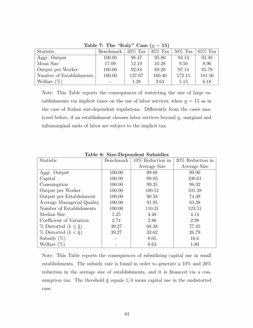
Table 7: The “Italy” Case (n = 15)Statistic Benchmark 20% Tax 35% Tax 50% Tax 65% TaxAggr. Output 100.00 98.47 95.80 94.14 92.48Mean Size 17.09 12.19 10.28 9.50 8.96Output per Worker 100.00 92.84 89.20 87.14 85.78Number of Establishments 100.00 137.07 160.40 172.15 181.56Welfare (%) - 1.28 3.63 5.15 6.18
Note: This Table reports the consequences of restricting the size of large es-
tablishments via implicit taxes on the use of labor services, when n = 15 as in
the case of Italian size-dependent regulations. Differently from the cases ana-
lyzed before, if an establishment chooses labor services beyond n, marginal and
inframarginal units of labor are subject to the implicit tax.
Table 8: Size-Dependent SubsidiesStatistic Benchmark 10% Reduction in 20% Reduction in
Average Size Average SizeAggr. Output 100.00 99.88 99.90Capital 100.00 99.93 100.61Consumption 100.00 99.35 98.32Output per Worker 100.00 100.51 101.28Output per Establishment 100.00 90.58 74.39Average Managerial Quality 100.00 91.95 83.38Number of Establishments 100.00 110.31 123.51Median Size 5.25 4.40 4.14Coefficient of Variation 2.74 2.86 2.98% Distorted (k ≤ k) 39.27 68.38 77.45% Distorted (k < k) 39.27 33.62 26.79Subsidy (%) - 8.05 16.6Welfare (%) - 0.63 1.80
Note: This Table reports the consequences of subsidizing capital use in small
establishments. The subsidy rate is found in order to generate a 10% and 20%
reduction in the average size of establishments, and it is financed via a con-
sumption tax. The threshold k equals 1/4 mean capital use in the undistorted
case.
44

References
Atkeson, A., & Kehoe, P. J. (2005). Modelling and Measuring Organization Capital. Journalof Political Economy, 113, 1026–1053.
Atkeson, A., Khan, A., & Ohanian, L. (1996). Are Data on Industry Evolution and GrossJob Turnover Relevant for Macroeconomics?. Carnegie-Rochester Conference Serieson Public Policy, 44, 215–239.
Baily, M. N., & Solow, R. M. (2001). International Productivity Comparisons Built fromthe Firm Level. Journal of Economic Perspectives, 15 (3), 151–172.
Basu, S., & Fernald, J. (1997). Returns to Scale in U.S. Production: Estimates and Impli-cations. Journal of Political Economy, 105 (2), 249–283.
Basu, S., Fernald, J., Oulton, N., & Srinivasan, S. (2003). The Case of Missing ProductivityGrowth: Or, Does Information Technology Explain Why Productivity Accelerated inthe United States But Not in the United Kingdom. NBER Working Paper 10010.
Beck, T., Demirguc-Kunt, A., & Levine, R. (2005). SMEs, Growth and Poverty: Cross-country Evidence. Journal of Economic Growth, 10 (3), 199–229.
Bergoeing, R., Kehoe, P., Kehoe, T., & Soto, R. (2002). A Decade Lost and Found: Mexicoand Chile in the 80’s. Review of Economic Dynamics, 5 (1), 166–205.
Bertola, G., Boeri, T., & Cazes, S. (1999). Employment Protection and Labor MarketAdjustment in OECD Countries: Evolving Institutions and Variable Enforcement.Employment and Training Papers 48, I.L.O.
Bertrand, M., & Kramarz, F. (2002). Does Entry Regulation Hinder Job Creation?. Quar-terly Journal of Economics, 117 (4), 1369–1413.
Blanchard, O., & Giavazzi, F. (2003). Macroeconomic Effects of Regulation and Deregulationin Goods and Labor Markets. Quarterly Journal of Economics, 118 (3), 879–908.
Burstein, A., & Monge, A. (2005). Aggregate Consequences of Foreign Firms in DevelopingCountries. Mimeo.
Caselli, F. (2004). Accounting for Cross-Country Income Differences. Forthcoming, Handbookof Economic Growth.
Caselli, F., & Gennaioli, N. (2002). Dynastic Management. mimeo.
Castaneda, A., Diaz-Gimenez, J., & Rios-Rull, J.-V. (2003). Accounting for Earnings andWealth Inequality. Journal of Political Economy, 111 (4), 818–857.
Castro, R., Clementi, G., & MacDonald, G. (2006). Legal Institutions, Sectoral Heterogene-ity, and Economic Development. manuscript, New York University.
45
Chang, R. (1998). Credible Monetary Policy in an Infinite Horizon Model: Recursive Ap-proaches. Journal of Economic Theory, 81 (2), 431–67.
Chang, Y. (2000). Wages, Business Cycles and Comparative Advantage. Journal of MonetaryEconomics, 46 (1), 143–171.
Chu, T. (2002). Exit Barriers and Productivity Stagnation. mimeo.
Cooley, T. F., & Prescott, E. C. (1995). Economic Growth and Business Cycles. In Cooley,T. F. (Ed.), Frontiers of Business Cycle Research, chap. 1. Princeton University Press,Princeton, New Jersey.
Cummins, J., & Violante, G. (2002). Investment-Specific Technical Change in the UnitedStates (1947-2000): Measurement and Macroeconomic Consequences. Review of Eco-nomic Dynamics, 5 (2), 243–284.
Davis, S., & Henrekson, M. (1999). Explaining National Differences in the Size and IndustryDistribution of Employment. Small Business Economics, 12 (1), 59–83.
Erosa, A., & Hidalgo, A. (2005). On Capital Market Imperfections as a Source of Low TFPand Economic Rents. Mimeo.
European Commission (1996). Enterprises in Europe (fourth report). Office for OfficialPublications of The European Communities, Luxembourg.
Flath, D. (2003). Regulation, Distribution Efficiency, and Retail Density. NBER WorkingPaper 9450.
Garibaldi, G., Pacelli, L., & Borgarello, A. (2003). Employment Protection Legislation andthe Size of Firms. IZA Discussion Papers 787.
Gollin, D. (1995). Do Taxes on Large Firms Impede Growth? Evidence from Ghana. Eco-nomic Development Center Papers 95-9, University of Minnesota.
Greenwood, J., Hercowitz, Z., & Krusell, P. (1997). Long-Run Implications of Investment-Specific Technological Change. American Economic Review, 87 (3), 342–62.
Greenwood, J., & Yorukoglu, M. (1997). 1974. Carnegie-Rochester Conference Series onPublic Policy, 46 (4), 49–95.
Guner, N., Ventura, G., & Yi, X. (2005). Macroeconomic Implications of Size-DependentPolicies. Mimeo. Pennsylvania State University.
Hall, R., & Jones, C. (1999). Why Do Some Countries Produce So Much More Output perWorker than Others?. Quarterly Journal of Economics, 114 (1), 83–116.
Henrekson, M., & Johansson, D. (1999). Institutional Effects on the Evolution of SizeDistribution of Firms. Small Business Economics, 12 (1), 11–23.
46

Herrendorf, B., & Teixeira, A. (2004). Barriers to Entry and Development. Mimeo, ArizonaState University.
Hopenhayn, H., & Rogerson, R. (1993). Job Turnover and Policy Evaluation: A GeneralEquilibrium Analysis. Journal of Political Economy, 101 (5), 915–938.
Ito, T. (1992). The Japanese Economy. MIT Press, Cambridge, Massachussets.
Kim, C. K. (2004). Developing on SME Development Policy for Indonesia: Drawing on theKorean Experience. U.N. Support Facility for Indonesia Recovery (UNSFIR) workingpaper.
Klenow, P., & Rodriguez-Clare, A. (1997). The Neoclassical Revival in Growth Economics:Has It Gone Too Far?. In Bernanke, B., & Rotemberg, J. (Eds.), NBER Macro Annual.MIT Press.
Krueger, A. (2002). Priorities for Further Reforms. In Krueger, A. (Ed.), Economic Reformsand the Indian Economy. University of Chicago Press, Chicago, Illinois.
Kumar, K., Rajan, R., & Zingales, L. (1999). What Determines Firm Size?. NBER WorkingPaper No. 7208.
Lagos, R. (2004). A Model of TFP. Federal Reserve Bank of Minneapolis Research Depart-ment Staff Report 345.
Lally, P. (2002). Fixed Assets and Consumer Durable Goods for 1925-2001. Survey ofCurrent Business, 23–37.
Larke, R. (1994). Japanese Retailing. Routledge, London and New York.
Lewis, W. (2004). The Power of Productivity: Wealth, Poverty and the Threat to GlobalStability. The University of Chicago Press.
Little, I., Mazumdar, D., & Page, J. M. (1987). Small Manufacturing Enterprises: A Com-parative Analysis of India and Other Economies. Oxford University Press for the WorldBank, New York.
Lucas, R. E. (1978). On the Size Distribution of Business Firms. Bell Journal, 9 (2), 508–523.
McCraw, T., & O’Brien, P. (1986). Production and Distribution: Competition Policy andIndustry Structure. In McCraw, T. (Ed.), America vs Japan. Harvard Business SchoolPress, Boston, Massachusetts.
McKinsey Global Institute (2000). Why the Japanese Economy is not Growing: Microbar-riers to Productivity Growth. McKinsey Global Institute.
Ministry of Economy, Trade and Industry (2004). 2004 White Paper on Small and MediumEnterprises in Japan. Japan Small Business Research Institute. Tokyo, Japan.
47

Mohan, R. (2002). Small-Scale Industry in India: A Critical Evaluation. In Krueger, A. (Ed.),Economic Reforms and the Indian Economy. University of Chicago Press, Chicago,Illinois.
Nicoletti, G., & Scarpetta, S. (2005). Regulation and Economic Performance: Product Mar-ket Reforms and Productivity in the OECD. OECD Economics Department WorkingPaper 460.
O.E.C.D. (2002). Small and Medium Enterprise Outlook. O.E.C.D. Publications, Paris.
Parente, S., & Prescott, E. (2000). Barriers to Riches. MIT Press, Cambridge, Mas-sachusetts.
Rauch, J. (1991). Modeling the Informal Sector Formally. Journal of Development Eco-nomics, 35 (1), 33–47.
Restuccia, D., & Rogerson, R. (2003). Policy Distortions and Aggregate Productivity withHeterogeneous Plants. Mimeo, University of Toronto.
Restuccia, D. (2004). Barriers to Capital Accumulation and Aggregate Total Factor Pro-ductivity. International Economic Review, 45 (1), 225–238.
Schmitz, J. (2001). Government Production of Investment Goods and Aggregate LaborProductivity. Journal of Monetary Economics, 47 (1), 163–187.
Tendulkar, S., & Bhavani, T. A. (1997). Policy on Modern Small Scale Industries: A Caseof Government Failure. Indian Economic Review, 32 (1), 39–64.
Tybout, J. (2000). Manufacturing Firms in Developing Countries: How Well Do they Do,and Why?. Journal of Economic Literature, 38 (1), 11–44.
U.S. Census Bureau (2002). Statistical Abstract of the United States: 2002. (122nd Edition),Washington, D.C.
U.S. Deparment of Commerce (2005). National Income and Product Accounts of the UnitedStates. Bureau of Economic Analysis. Available at www.bea.gov.
Veracierto, M. (2001). Employment Flows, Capital Mobility, and Policy Analysis. Interna-tional Economic Review, 42 (3), 571–596.
World Bank (2000). Small and Medium Enterprises in Argentina. Report No. 22803-AR,Washington D.C.
48


