
Macroeconomics
for Emerging East Asia
Calla Wiemer
26 November 2017
9. Models of Equilibrium and Disequilibrium
Classical School
Income–Expenditure Model
Consumption Function and Planned Expenditures
Persistence of Unemployment
Demand Stimulus Policies
The Multiplier
Aggregate Demand / Aggregate Supply Model
Aggregate Demand
Aggregate Supply
Recession
Demand Stimulus Policies
IS-LM Model
Marginal Efficiency of Capital and the IS Curve
Liquidity Preference and the LM Curve
Equilibrium in Income and the Interest Rate
External Balance and the Mundell-Fleming Extension
Evolving Schools of Thought
Data Note
Bibliographic Note
Bibliographic Citations
List of Boxes
9.1 Calculating the expenditures multiplier
9.2 What else Keynes said
List of Figures
9.1 Income-Expenditure Model
9.2 Demand Stimulus Policies in the I-E Model
9.3 Aggregate Demand / Aggregate Supply Model
9.4 Recession in the AD/AS Model
9.5 Monetary Stimulus in the AD/AS Model
9.6 IS-LM Model
9.7 Mundell-Fleming Model

1
9. Models of Equilibrium and Disequilibrium
Macroeconomic models provide a framework for relating key aggregate
magnitudes: output; income; the price level; unemployment; the wage rate;
consumption; investment; government spending and taxation; the money
supply; the interest rate; international trade and capital flows; and the
exchange rate. Classical and Keynesian models diverge on how quickly
prices and wages adjust to eliminate the twin excess supplies
characteristic of a downturn – a glut in product markets and unemployed
workers in labor markets. With that, the two schools reach different
conclusions on policy.
Schools of thought within macroeconomics diverge in how they regard the market
clearing process. The Classical School and its heirs view markets as well-functioning and
resilient in response to shocks. The constant hammering of shocks gives rise to fluctuations, to
be sure, but these are seen as healthy coping mechanisms in support of vibrant economic growth.
Under the Classical paradiagm, macroeconomic policy intervention only adds to uncertainty and
impedes the adjustment process. By contrast, the Keynesian School and its offshoots view
economic slumps as serious, inexorable, and not self-correcting in any timely fashion.
Keynesians favor an active government role in hastening recovery from downturns and in
maintaining stability more generally.
The comparative static analysis of this chapter rests on the theoretical construct of
equilibrium. In the standard microeconomic application, a market in equilibrium at some price
and quantity is subjected to an exogenous shock – a curve shifts and a new equilibrium price and
quantity emerge. Comparative statics is a useful analytical tool when the passage of time can be
suppressed and the process of transition is not of interest for the purpose at hand.
In macroeconomics, however, the main concern is with instability and disequilibrium.
Output fluctuates over time; the labor market fails to clear; and inflation is prone to rearing up.
We leave the dynamic analysis of business cycles to the next chapter. In this chapter we focus on
static models of aggregate economic activity devised to illuminate deviations from trend, either
through disequilibrium being sustained in the Keynesian mode or through adjustment to changes
in equilibrium conditions yielding an erratic growth path under the Classical framework.
The first section reviews the basic tenets of the Classical School. The second presents the
Income-Expenditure Model inspired by Keynes. This is a disequilibrium model in the sense that
excess capacity persists as prices and wages fail to adjust to clear markets within the time frame
of the analysis. The Aggregate Demand / Aggregate Supply Model of the third section joins a
short-run period in which wages are sticky and a long-run period in which wages and prices fully
adjust. This model tracks the interplay of the price level and aggregate output as the response to
shock plays out in the short and long runs. The fourth section introduces a more elaborate
interpretation of Keynesian disequilibrium in the IS-LM model (the notation referring to
investment, saving, liquidity, and money) and outlines its extension to an open-economy context
2
with the Mundell-Fleming Model. Finally, the fifth section summarizes the evolution in Classical
versus Keynesian based schools of thought as manifested in contemporary Dynamic Stochastic
General Equilibrium Models.
Classical School
The first challenge for economics as a discipline is to explain how a market economy
manages to achieve as much success as it does. Most people most of the time are put to work
productively. Investment funds find their way into financing projects of a range of durations and
risk profiles. Entrepreneurs develop new products and technologies and devise new ways of
doing business. Economies grow and advance over time. The Classical School offered insight
into understanding this success. The story is one of prices equilibrating demands and supplies to
allocate resources to the uses in which they are most highly valued.
The principle of equilibration that applies to individual markets can be extended to an
economy as a whole. Adjustment of wages ensures full employment. Adjustment of interest rates
matches saving with investment. An unbroken circle links production to income to spending on
what has been produced. Say’s Law, named for early 19th
century French economist Jean-
Baptiste Say, captures this succinctly: Supply creates its own demand.
The full employment equilibrium of the Classical paradigm is formulated in real terms.
Money does not figure in. Only relative prices matter. Any good could be chosen as numeraire
with the value of everything else expressed in terms of that referent. Introducing money provides
a convenient unit of account, but its impact on resource utilization is held to be neutral. Doubling
the supply of money simply reduces its value by half in terms of everything else as all prices
double. No role is seen for credit expansion to boost real economic activity. When an economy
operates inherently at full employment, credit infusions simply lead to higher prices.
Classical economic theory does well in explaining the impressive achievements of a
market economy in yielding efficient utilization of resources and weathering shocks. The
Classical paradigm, however, was hard pressed to explain the Great Depression of the 1930s.
This terrible cataclysm sparked a revolution in economic thought.
Income–Expenditure Model
The Great Depression was a worldwide economic disaster of incomparable proportions.
Although a number of other countries fell into recession sooner, the U.S. suffered the longest and
deepest downturn. Unemployment reached 25 percent of the labor force. More than a third of all
banks failed. Output declined by 30 percent, and by the end of the 1930s had still not recovered
to the level of 1929. Globally, the contraction was compounded by the piling on of tariff barriers
such that international trade plummeted by two-thirds.
John Maynard Keynes stepped up to meet the intellectual challenge of explaining,
counter to Classical doctrine, how an economy can become mired in recession. His General
Theory of Employment, Interest, and Money was published in 1936. The Income-Expenditure
Model is the simplest formalization of Keynes’s argument. We first develop the key functional
relationships of the model. We then apply the model to explaining persistent unemployment. In

3
Keynes’s view, the way to catalyze recovery is through government fiscal action. We proceed to
examine the mechanics of such demand stimulus policies and the impact of the Keynsian
expenditures multiplier.
Consumption Function and Planned Expenditures
The Income-Expenditure Model turns on the relationship between consumption and
income. Consumption by households is assumed to increase with income, but by less than the
full measure of income. That part of income not spent on consumption is saved. Specifying the
consumption function in linear form and expressing income as net of taxes, which for simplicity
are assumed not to depend on income, we have:
𝐶 = 𝐶0 + 𝛽(𝑌 − 𝑇),
where C = consumption by households;
C0 = autonomous consumption (consumption when income is zero);
Y = income;
𝑇 = taxes (the bar indicates exogeneity);
β = marginal propensity to consume (MPC).
The marginal propensity to consume, β, is the slope of the consumption function, or the ratio of a
change in consumption to a change in income, ΔC/ΔY. Logically, β must take on a value between
zero and one.
The Keynesian consumption function frames economic behavior in a fundamentally
different way from Say’s Law. Say’s Law is premised on all income being spent. That part of
income not directed toward consumption is expected to be absorbed by investment via the
market for loanable funds. In the Keynesian scheme of things, by contrast, saving depends not on
the interest rate but on income as the counterpart to consumption. Planned investment is treated
as independent of current income, motivated rather by expectations about the future. Unplanned
investment in the form of changes in inventories is, however, regarded as critically dependent on
income as will be explained.
The specification of planned expenditures follows the expenditures approach to
measuring GDP detailed in Chapter 4. All elements other than consumption are taken as
exogenous as noted with an overbar. Inserting the consumption function specified above into the
expenditures equation for GDP yields:
Planned Expenditures = 𝐶0 + 𝛽(𝑌 − 𝑇) + 𝐼 + 𝐺 + 𝑋 − 𝑀,
where 𝐼 = planned investment;
𝐺 = government spending;
𝑋 = exports;
𝑀 = imports.

4
This expression for planned expenditures represents the aggregate demand side of the Income-
Expenditure Model.
Persistence of Unemployment
The aggregate supply side of the model is given by the value of output produce which is
identically equal to the income earned in the production process. The question to be examined by
the model is: What happens when the income earned in production does not generate sufficient
demand to purchase the output supplied?
Figure 9.1 captures the story as
depicted by Samuelson (1948). The
model is sometimes referred to as the
“Keynesian Cross”. Planned expenditures
are an increasing function of income with
slope given by the MPC at less than one.
The 45 degree line, with slope of one,
represents all income, absorbed as it must
be in realized expenditures which are
defined to include unplanned inventory
accumulation or decumulation. Thus
realized expenditures are equal to output
which is in turn equal to income. The
level of output that provides full
employment is given by an income of YFE. At YFE as depicted, planned expenditures
fall short of output produced. The result
is the unplanned accumulation of
inventory. This inventory build-up
prompts producers to lay off workers and
cut back production. Only when income
drops to Y* does the economy generate
planned expenditures sufficient to clear the market of output produced with any inventory
changes matching producer intentions. At income of less than Y*, inventories are drawn down
motivating producers to expand output and income payments.
Alignment between saving and investment in this model (where saving, S, subsumes any
cross-border inflows or outflows such that S = I + X – M as explained in Chapter 5) is achieved
not through interest rate equilibration as in the Classical model but through unplanned inventory
changes. Saving and planned investment may differ ex ante. But ex post, any saving in excess of
planned investment will find expression in the unplanned pile up of inventories.
An equilibrium of sorts is achieved at Y* in that there is no tendency for change within
the structure of the model. Yet this outcome is characterized by persistent unemployment. The
labor market does not clear. In a broader sense, then, markets are in a state of disequilibrium.
Classical theory holds that the wage rate should fall to eliminate the gap between those supplying
labor and those demanding it. In the Keynesian world, however, wages are sticky. Workers resist
9.1 Income-Expenditure Model
5
cuts in pay and employers are loath to impose them. The alternative of cutting jobs in the face of
a slowdown in sales is more palatable. Moreover, Keynesians argue that any cut in wages would
only exacerbate the deficiency of aggregate demand on product markets as with lower wages
consumers have less income to spend. For Keynesians the solution to depressed economic
conditions is to be found in government stimulus policies.
Demand Stimulus Policies
The Keynesian story of economic underperformance rests on insufficient aggregate
demand. More spending would induce more production and higher employment. Government is
able to provide the boost in spending an economy needs, either by increasing its outlays directly
or by reducing taxes so that households can take on the spending.
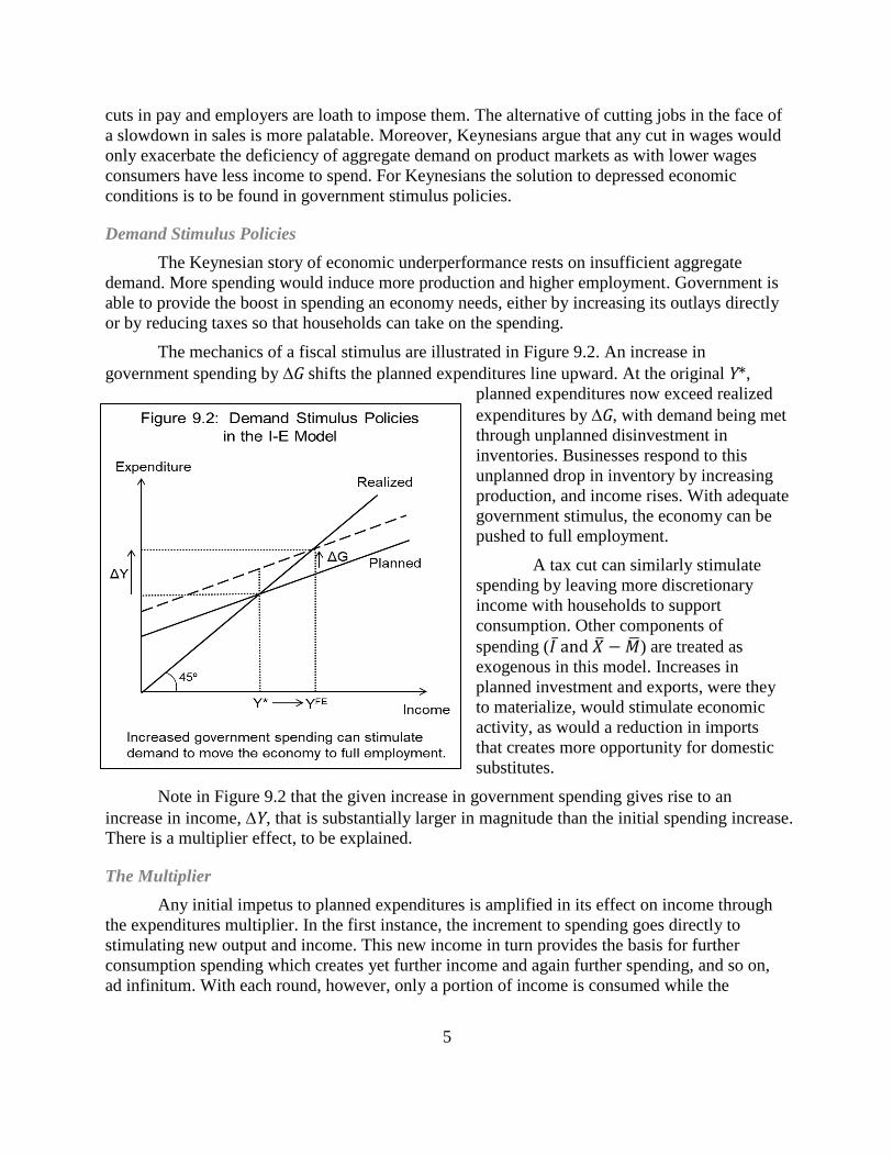
The mechanics of a fiscal stimulus are illustrated in Figure 9.2. An increase in
government spending by G shifts the planned expenditures line upward. At the original Y*,
planned expenditures now exceed realized
expenditures by G, with demand being met
through unplanned disinvestment in
inventories. Businesses respond to this
unplanned drop in inventory by increasing
production, and income rises. With adequate
government stimulus, the economy can be
pushed to full employment.
A tax cut can similarly stimulate
spending by leaving more discretionary
income with households to support
consumption. Other components of
spending (𝐼 ̅and �̅� − �̅�) are treated as
exogenous in this model. Increases in
planned investment and exports, were they
to materialize, would stimulate economic
activity, as would a reduction in imports
that creates more opportunity for domestic
substitutes.
Note in Figure 9.2 that the given increase in government spending gives rise to an
increase in income, Y, that is substantially larger in magnitude than the initial spending increase.
There is a multiplier effect, to be explained.
The Multiplier
Any initial impetus to planned expenditures is amplified in its effect on income through
the expenditures multiplier. In the first instance, the increment to spending goes directly to
stimulating new output and income. This new income in turn provides the basis for further
consumption spending which creates yet further income and again further spending, and so on,
ad infinitum. With each round, however, only a portion of income is consumed while the
9.2 Demand Stimulus Policies in the I-E Model

6
remainder is saved. Thus with each round the increment to spending gets smaller such that the
total impact approaches a definable limit. The math is laid out in Box 8.1.
A word of caution on the Keynesian remedy to a slump is in order. While increasing
government spending and cutting taxes to stimulate an economy may find ready political appeal,
the burden of the public debt can weigh against over reliance on Keynesian fiscal policies.
Nevertheless, it is possible to raise spending and taxes by equal amounts and still deliver a
stimulus within the framework of the Income-Expenditure Model. This is because some of the
tax revenue diverted from private parties would have been saved and thus would not have
contributed to aggregate demand whereas the government can act to spend all of it.
Aggregate Demand / Aggregate Supply Model
The Income-Expenditure Model discussed in the preceding section treats income and
consumption as endogenous variables and explains how an economy can fall short of operating
at its potential with no tendency for any timely recovery. All pricing variables, including the
wage rate, the interest rate, and the exchange rate, are implicitly held fixed. In the long run, of
Box 9.1: Calculating the expenditures multiplier
Suppose a government undertakes a stimulus project involving an investment in public
infrastructure launched with an outlay represented by ΔG. That ΔG in spending goes toward
contracting work by engineering and construction firms, purchasing materials, and employing civil servants to engage in management and oversight. The spending feeds into incomes in all forms: wages, interest, rents, and profits. In turn, the recipients of these income streams will spend part on consumption and save part. The part spent on consumption then fuels a new round of income increases which generates more consumption and yet more income, and so on.
To trace the ultimate impact on income of the initial spending increase, let us formalize the series of spending increments round by round. At each round, a share of income from the last round equal to the marginal propensity to consume (MPC) becomes new spending.
Round 1 ΔG
Round 2 MPC • ΔG
Round 3 MPC2 • ΔG
Round 4 MPC3 • ΔG
⁞ ⁞
Thus the increase in income that follows from an increase in government spending is given as:
ΔY = (1 + MPC + MPC2 + MPC
3 + … ) • ΔG.
Because MPC takes on a value between zero and one, each time the ratio is raised to a higher power the resulting increment is diminished in magnitude. The elements of the series thus approach zero. Algebraically, the sum of the elements of the infinite series is equivalent to 1/(1-MPC). The magnitude in the denominator, 1-MPC, is the marginal propensity to save.
The higher the MPC, the greater the impact of a fiscal stimulus. For an MPC of 0.8, for example, the multiplier is 5. For an MPC of 0.5, the multiplier is only 2.
9.1 Calculating the expenditures multiplier

7
9.3 Aggregate Demand / Aggregate Supply
Model
course, prices are flexible and will function to resolve demand and supply mismatches. The
model of aggregate demand and aggregate supply is an effort to bridge a short-run period when
market response to shock is limited and the long-run time frame when an equilibrium is achieved.
Similar to the model of demand and supply in a particular market, the Aggregate Demand
/Aggregate Supply Model focuses on the interaction between prices and quantities. We develop
first the demand side, then the supply side. Once the model is formulated, we apply it to
analyzing both a recessionary shock and the implementation of government stimulus policies.
Aggregate Demand
The aggregate demand function relates real demand for all final goods and services in an
economy to the general price level. As with demand in a particular market, the relationship is
inverse such that a rising price level is associated with a declining demand for real output. The
reasons for a downward sloping demand curve on the aggregate level are different from those for
a single market, however. First, the real balance effect (also known as the Pigou effect) holds
that as prices rise, the purchasing power of given money holdings decreases to cause a decline in
demand. Second, the interest rate effect rests on the Keynesian notion of a trade-off between
holding liquid money balances to support transactions and tying up wealth in bonds. As prices
rise, the need to keep more cash on hand diverts funds out of bonds causing the interest rate to
rise which then restrains investment spending. Finally, the exchange rate effect notes that higher
domestic prices act to increase the real exchange value of the local currency causing demand for
imports to rise and for exports to fall which further undermines demand for home produced
goods and services.
Changes in factors other than price
that bear on the components of spending
(consumption, investment, government,
exports, and imports) cause the aggregate
demand curve to shift. Important among
these factors are expectations about the
future, availability of credit, political forces,
and global economic conditions.
Aggregate Supply
On the supply side, the short run
response to changes in the price level differs
from the long run response, as indicated in
Figure 9.3. The economy depicted is in a
state of both long-run and short-run
equilibrium at Q* and P*.
In the long run, the supply curve is
vertical. This is because in the long run
production capacity is determined solely by
real factor inputs and technology, not by the
price level. With capacity given by Q*, and
8
the money supply set exogenously, prices, given time, will arrive at the level, P*, that ensures
full employment of resources.
In the short run, shocks can move the economy away from normal capacity operation.
Product markets are on the front lines in absorbing shocks. The transmission of the impact to
labor markets takes time as terms of compensation are slow to be revisited and revised. Thus in
the short run following a shock, real wages will diverge from their long-run equilibrium level.
Following a shock that raises output prices, workers will only gradually realize that the
purchasing power of their wages has been eroded. Seeking and securing wage increases is a
protracted process. In the short run then, price increases result in lower real wages to workers
and higher profits to producers. Producers respond by increasing output, which means drawing
more people into paid labor and/or boosting worker hours. The economy moves upward along
the short-run supply curve. With further passage of time, however, competition in the labor
market as producers seek to expand hiring will drive up wages. Profits will then fall back to
normal, and the economy will return to its long-run supply curve.
We proceed to apply the model, tracing the response in output and prices to changes in
external forces.
Recession
The biggest source of macroeconomic volatility lies with investment demand. Investment
is motivated by expectations of future profit, with time horizons that can run to decades.
Willingness to take on risk is buffeted by sentiment about future prospects which can swing
wildly between optimism and pessimism on a mass scale. Bad times tend to breed ever more
doubt, good times ever more euphoria. When an economy overshoots on the upside, the
downturn that follows can be sharp.
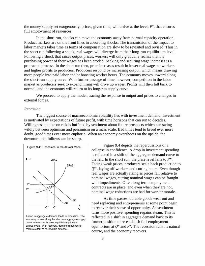
Figure 9.4 depicts the repercussions of a
collapse in confidence. A drop in investment spending
is reflected in a shift of the aggregate demand curve to
the left. In the short run, the price level falls to P*′. Facing weak prices, producers scale back production to
Q*′, laying off workers and cutting hours. Even though
real wages are actually rising as prices fall relative to
nominal wages, cutting nominal wages can be fraught
with impediments. Often long-term employment
contracts are in place, and even when they are not,
nominal wage reductions are bad for worker morale.
As time passes, durable goods wear out and
need replacing and entrepreneurs at some point begin
to recover their sense of opportunity. As sentiment
turns more positive, spending regains steam. This is
reflected in a shift in aggregate demand back to its
former position to re-establish full-employment
equilibrium at Q* and P*. The recession runs its natural
course, and the economy recovers.
9.4 Recession in the AD/AS
Model

9
Demand Stimulus Policies
Governments seek to maintain economic stability through the application of monetary
and fiscal policies. A monetary stimulus works through the injection of reserves into the banking
system that drive new lending. The ramifications are shown in Figure 9.5. Let us take as a
starting point an economy at long run equilibrium given by P* and Q*. The increase in spending
stimulated by the expansion in credit shifts the aggregate demand curve to the right. The price
level rises to P*′ pushing the economy along its short run aggregate supply curve. Rising prices
relative to given wages drive profit growth motivating producers to expand production. Output
increases to Q*′. With time, however, workers react to rising prices with demands for higher
nominal wages to preserve the real purchasing power of their pay. The increase in production
costs is captured by a shift in the short-run supply curve to the left. As real wages regain their
equilibrium level, the economy returns to its long-run aggregate supply curve with output at Q*
but with the price level now at P*′′. The monetary stimulus thus achieves only a temporary
increase in output while the effect on prices is lasting.
A fiscal stimulus, involving increased
government spending or reduced taxes, is
represented with the same initial rightward shift
in aggregate demand as in Figure 9.5. As the
government competes with the private sector for
goods and services, prices are bid up and
profitable opportunities abound. The economy
goes into overdrive. Once the spending spree
runs its course, however, aggregate demand
drops back and the economy reverts to its
original equilibrium output and price level.
Stimulus action undertaken, as just
outlined, when an economy is functioning at full
capacity has only a fleeting effect on output. In
the case of a monetary stimulus, the increase in
prices is nevertheless enduring. In the case of a
fiscal stimulus, any borrowing associated with
spending increases or tax reductions results in a
higher debt burden. This long-run consequence
must be taken into account in assessing the merits of short-term stimulus gains. However, if the
starting point is one of less than capacity operation, as in Figure 9.4 at P*′ and Q*′, and the
recovery process, however foreordained, is protracted, stimulus policies may hold appeal for
their catalytic power. Giving a stalled economy a jumpstart and shortening the time needed to
regain full employment, if this can be achieved at tolerable cost to the fiscal budget and minimal
impact on prices, represents the ultimate in successful macroeconomic policy.
IS-LM Model
In a Keynesian world, markets do not adjust quickly to reach equilibrium. Indeed, during
the time frame addressed, a disequilibrium stasis can take hold. Unemployment persists, and
9.5 Monetary Stimulus in the AD/AS
Model
10
production capacity sits idle. The crux of the problem is that aggregate demand at the full
employment level of income is insufficient to induce that level of output and income. The
Income-Expenditure Model suppresses prices and wages to cast demand purely as a function of
income. By contrast, the Aggregate Demand / Aggregate Supply Model allows for quick
adjustment of output prices in response to shocks but assumes stickiness in wages to describe a
process of equilibration that plays out over time. The IS/LM model formulated by Hicks (1937)
resembles the Income/Expenditure Model in that neither prices nor wages adjust quickly to clear
markets leaving output short of potential and workers out of jobs.
The new element in the IS-LM model is an endogenous interest rate which serves as the
fulcrum of macroeconomic adjustment to shock. The interest rate affects the economy through
two channels. One is real investment spending. The other is the allocation of financial assets
between liquid money balances and bonds. We consider each of these channels in turn, then
bring them together to explain their joint determination of aggregate output. The model as
originally conceived pertains to a closed economy. The Mundell-Fleming Model, which we
outline briefly, extends the framework to an open economy.
Our treatment of the IS-LM and Mundell-Fleming Models is cursory. A thorough
understanding would require working through comparative static exercises to trace the impact of
external shocks, including, importantly, monetary and fiscal policy actions. For our purposes in
developing a macroeconomics for Emerging East Asia, models that focus exclusively on a
domestically determined market rate of interest are of limited applicability. A better fit is a
model that incorporates managed exchange rates, which we develop in Chapter 13. Nevertheless,
to varying degrees in the economies of Emerging East Asia, domestic interest rates do play a role
in macroeconomic performance. Hence, we outline the structure of the arguments.
Marginal Efficiency of Capital and the IS Curve
The IS curve defines pairs of income (equal to output) and the interest rate that equate
investment and saving. Investment is assumed to depend negatively on the interest rate. Simply
put, this is because as the interest rate falls, more investment projects become viable. Keynes
formalized the argument with his concept of a declining marginal efficiency of capital – the
more extensive is investment at a given point in time, the lower is the return to the marginal unit
of investment. This is due to diminishing marginal productivity of capital as capital becomes
more abundant relative to other factors of production, given the state of technology. A lower
interest rate increases the rate of return net of borrowing costs for the entire schedule of possible
investment levels such that at the margin some projects that would not have been pursued at a
higher rate of interest will be undertaken. Saving and consumption are assumed to depend on
income in standard Keynesian fashion.
To capture the investment/saving side of the IS-LM Model, we rewrite the Keynesian
expenditure equation expressing investment as a function of the interest rate and setting
expenditures equal to income:
𝑌 = 𝐶0 + 𝛽(𝑌 − 𝑇) + 𝐼(𝑟) + 𝐺 + 𝑋 − 𝑀,
where r = the interest rate.
11
To preserve the equality, an increase in I, following from a decrease in r, must be
matched by an increase in Y sufficient to yield the necessary saving to support the higher I. Conversely, an increase in the interest rate inhibits investment which causes a decline in income
sufficient to realign lower saving with the lower investment. Note that preservation of the
saving/investment balance is implicitly ensured within the IS equation since Y minus all terms on
the right hand side other than I(r) is equal to saving (where government spending is treated as
public consumption).
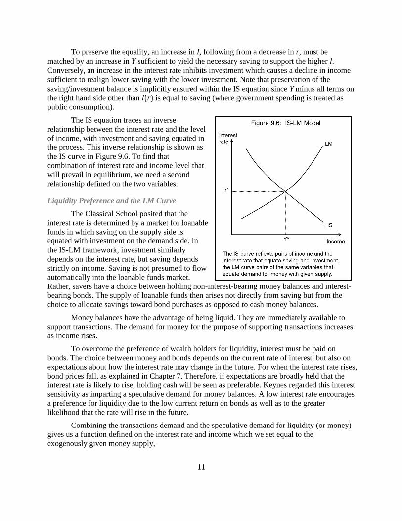
The IS equation traces an inverse
relationship between the interest rate and the level
of income, with investment and saving equated in
the process. This inverse relationship is shown as
the IS curve in Figure 9.6. To find that
combination of interest rate and income level that
will prevail in equilibrium, we need a second
relationship defined on the two variables.
Liquidity Preference and the LM Curve
The Classical School posited that the
interest rate is determined by a market for loanable
funds in which saving on the supply side is
equated with investment on the demand side. In
the IS-LM framework, investment similarly
depends on the interest rate, but saving depends
strictly on income. Saving is not presumed to flow
automatically into the loanable funds market.
Rather, savers have a choice between holding non-interest-bearing money balances and interest-
bearing bonds. The supply of loanable funds then arises not directly from saving but from the
choice to allocate savings toward bond purchases as opposed to cash money balances.
Money balances have the advantage of being liquid. They are immediately available to
support transactions. The demand for money for the purpose of supporting transactions increases
as income rises.
To overcome the preference of wealth holders for liquidity, interest must be paid on
bonds. The choice between money and bonds depends on the current rate of interest, but also on
expectations about how the interest rate may change in the future. For when the interest rate rises,
bond prices fall, as explained in Chapter 7. Therefore, if expectations are broadly held that the
interest rate is likely to rise, holding cash will be seen as preferable. Keynes regarded this interest
sensitivity as imparting a speculative demand for money balances. A low interest rate encourages
a preference for liquidity due to the low current return on bonds as well as to the greater
likelihood that the rate will rise in the future.
Combining the transactions demand and the speculative demand for liquidity (or money)
gives us a function defined on the interest rate and income which we set equal to the
exogenously given money supply,
9.6 IS-LM Model
12
�̅�𝑆 = 𝐿(𝑟, 𝑌),
where �̅�𝑆 = exogenous money supply;
L(•) = the liquidity preference function.
The function L(r, Y) depends negatively on r and positively on Y. The LM equation yields pairs
of r and Y at which the public is willing to hold the available supply of money.
For given �̅�𝑆, we can trace a relationship that must hold between r and Y. An increase in
income will tend to increase the demand for liquidity for transactions purposes. To offset this,
the interest rate must rise to induce the holding of bonds as an alternative to money. Thus the
relationship between r and Y that preserves a given value for money demand, which will align it
with money supply, is positive. This is represented by the upward sloping LM curve of Figure
9.6.
Equilibrium in Income and the Interest Rate
The IS and LM curves of Figure 9.6 jointly determine equilibrium values of income and
the interest rate. Pairs of r and Y along the IS curve equate saving and investment. Pairs of the
same variables along the LM curve preserve a given level of money demand set equal to an
exogenously controlled money supply.
True to form in a model of Keynesian inspiration, the equilibrium income given by Y* in
Figure 9.6 need not represent a full-employment outcome. The economy can be operating at less
than capacity with unemployment manifest at Y* with no impetus for output and income to
increase. In the IS-LM Model, both fiscal and monetary policy offer the potential to boost
equilibrium output. A detailed exposition of the mechanics is beyond the scope of this text. In
brief, expansionary fiscal policy involving government spending increases or tax cuts shifts the
IS curve to the right pushing up the interest rate as income rises. The upward movement along
the LM curve ensures equality between money demand and fixed money supply as the
combination of higher income and higher interest rate have offsetting effects on money demand
(higher income raising it, a higher interest rate lowering it). Expansionary monetary policy shifts
the LM curve to the right driving the interest rate downward as income rises. The lower interest
rate ensures that investment spending will pick up to match the increase in saving that follows
from higher income.
External Balance and the Mundell-Fleming Extension
The basic IS-LM Model assumes a closed economy, or at least takes international trade
and financial flows as fixed. The Mundell-Fleming Model incorporates an endogenous foreign
sector into the analysis. The balance on the current account is assumed to be a function of
income and on the financial account a function of the interest rate. As income increases, imports
rise and exports decline in response to the increase in domestic demand. Hence the balance on
the current account decreases (a surplus shrinks or a deficit expands). As the interest rate rises
domestically, more capital flows in and less flows out. The balance on the financial account thus
increases (a surplus expands or a deficit shrinks). An increased surplus on one account must be
matched by an increased deficit on the other to preserve overall balance.
13
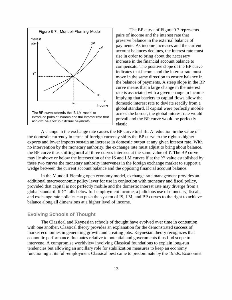
The BP curve of Figure 9.7 represents
pairs of income and the interest rate that
preserve balance in the external balance of
payments. As income increases and the current
account balances declines, the interest rate must
rise in order to bring about the necessary
increase in the financial account balance to
compensate. The positive slope of the BP curve
indicates that income and the interest rate must
move in the same direction to ensure balance in
the balance of payments. A steep slope in the BP
curve means that a large change in the interest
rate is associated with a given change in income
implying that barriers to capital flows allow the
domestic interest rate to deviate readily from a
global standard. If capital were perfectly mobile
across the border, the global interest rate would
prevail and the BP curve would be perfectly
elastic.
A change in the exchange rate causes the BP curve to shift. A reduction in the value of
the domestic currency in terms of foreign currency shifts the BP curve to the right as higher
exports and lower imports sustain an increase in domestic output at any given interest rate. With
no intervention by the monetary authority, the exchange rate must adjust to bring about balance,
the BP curve thus shifting until all three curves intersect at the same value of Y. The BP curve
may lie above or below the intersection of the IS and LM curves if at the Y* value established by
these two curves the monetary authority intervenes in the foreign exchange market to support a
wedge between the current account balance and the opposing financial account balance.
In the Mundell-Fleming open economy model, exchange rate management provides an
additional macroeconomic policy lever for use in conjuction with monetary and fiscal policy,
provided that capital is not perfectly mobile and the domestic interest rate may diverge from a
global standard. If Y* falls below full-employment income, a judicious use of monetary, fiscal,
and exchange rate policies can push the system of IS, LM, and BP curves to the right to achieve
balance along all dimensions at a higher level of income.
Evolving Schools of Thought
The Classical and Keynesian schools of thought have evolved over time in contention
with one another. Classical theory provides an explanation for the demonstrated success of
market economies in generating growth and creating jobs. Keynesian theory recognizes that
economic performance fluctuates relative to potential and governments thus find scope to
intervene. A compromise worldview involving Classical foundations to explain long-run
tendencies but allowing an ancillary role for stabilization measures to keep an economy
functioning at its full-employment Classical best came to predominate by the 1950s. Economist
9.7 Mundell-Fleming Model
14
Paul Samuelson dubbed this the “Neoclassical Synthesis” in the third edition of his best selling
principles text.
The Neoclassical Synthesis represented a moderation of the more radical stand Keynes
took in the General Theory. Keynes saw demand shortfall as a chronic and pernicious malady of
the capitalist system. His concerns led him to argue “that the duty of ordering the current value
of investment cannot safely be left in private hands” (p. 164), and consequently “that a somewhat
comprehensive socialisation of investment will prove the only means of securing an
approximation to full employment” (p. 375). For more on Keynes’s not so prescient musings on
the fate of private investment and the “euthanasia of the rentier”, along with a digression into his
more prophetic warnings on war reparations, see Box 8.2.
Criticisms laid against Keynesianism on theoretical grounds, in conjunction with the play
of events in the 1970s, led to a waning of influence in this school of thought. The lack of
microeconomic foundations to explain why wages and prices should fail to clear markets was a
vulnerability. Firms and households were assumed to behave rationally in trading labor and
commodities at a micro level, yet they were purportedly unable to adjust to changing
circumstances at the macro level. Keynesian advocacy of fiscal stimulus to overcome weak
demand was also subject to attack. Increases in government spending were presumed to impact
the economy with a multiplier effect as new spending generated new income which in turn
triggered new spending and so forth. Theories of consumption developed by Friedman (1957)
and Modigliani (1966), however, maintained that changes in consumption habits were not so
easily dislodged from patterns based on long term earnings prospects and that income regarded
as transitory would mostly be saved. The supposed multiplier effect would thus dissipate quickly.
Finally, on practical grounds, if markets were prone to malfunctioning, policy was not less so.
Lags in implementation and results were long and variable. Moreover, the politics of stimulus
and restraint were asymmetrical. Fiscal budgets once unbalanced were hard to rebalance and
credit having been unleashed was tough to reign back in.
The undoing of the Keynesian revolution was wrought by the simultaneous emergence of
stagnant growth and high inflation – stagflation – in the US in the 1970s. Stagnant growth with
its accompanying high unemployment was in principle supposed to forestall upward pressure on
wages and prices. This breech of the Keynesian order provided the opening for the Classical
school to regain the ascendency by offering an explanation of events that rested on explicit
microeconomic foundations. If employers expected output prices to rise at a given rate, they
would be prepared to raise wages by that rate, while workers expecting their cost of living to rise
at the going rate would demand the very wage increases employers were prepared to offer.
Markets would clear based on rational expectations on the part of economic agents. The
consequences of shocks, including any demand stimulus measures implemented by the
government, were foreseeable and were thus incorporated into supply and demand behavior.
Within this framework, observed reductions in employment during a downturn were interpreted
as the result of calculated choice. Under the various monikers of New Classical Economics or the
Rational Expectations School or Real Business Cycle Theory, econometric models were
constructed on the premise of market equilibration and found to closely replicate observed
features of the typical business cycle.

15
9.2 What else Keynes said
Box 8.2: What else Keynes said
Long before he wrote the General Theory, Keynes had achieved considerable stature not only as an economic theoretician but as a voice in world affairs. His Economic Consequences of the Peace, written in 1919, was a polemic against the spoliation of Germany by the victors of World War I. Keynes felt so strongly about this issue that he withdrew as an advisor to the peace negotiations in protest against a treaty he believed would “sow the decay of the whole of civilized Europe.” (p. 225)
In his writing, Keynes developed the empirical case that Germany’s capacity to pay reparations fell far short of the terms imposed by the Treaty of Versailles. He argued further that for Germany to make payments even on the order he was proposing, the country’s exports would have to increase and imports decrease greatly to generate the necessary foreign exchange. This could happen only if Western Europe and the US opened their own markets to German products and faced up to greater competition from German goods worldwide. Keynes advocated an alternative proposal whereby the U.S. would forgive the debts it was owed by Britain, France, and Italy, and these countries would in turn scale back greatly their demands on Germany.
Keynes wrote ardently:
“I believe that the campaign for securing out of Germany the general costs of the war was one of the most serious acts of political unwisdom for which our statesmen have ever been responsible. To what a different future Europe might have looked forward if either [British Prime Minister] Mr. Lloyd George or [U.S. President Mr. Woodrow] Wilson had apprehended that the most serious of the problems which claimed their attention were not political or territorial but financial and economic, and that the perils of the future lay not in frontiers or sovereignties but in food, coal, and transport. … [T]he financial problems which were about to exercise Europe could not be solved by greed. The possibility of their cure lay in magnanimity.” (pp. 146-147)
The book became an international best seller – arriving too late, however, to alter history’s harrowing course toward Nazism and another world war. Yet in the aftermath of World War II, the lessons had seemingly been absorbed. The U.S. dedicated enormous sums to the post-war reconstruction of Europe and Japan, launching an era of prosperity that redounded to all.
For all his brilliance, Keynes was not without ideas that failed to withstand the test of time. One
of his odder notions in hindsight was that continued capital accumulation would lead to a day when the return on capital would fall to zero and result in the “euthanasia of the rentier” with profound implications for social organization. From the General Theory:
“If I am right in supposing it to be comparatively easy to make capital-goods so abundant that the marginal efficiency of capital is zero, this may be the most sensible way of gradually getting rid of many of the objectionable features of capitalism. For a little reflection will show what enormous social changes would result from a gradual disappearance of a rate of return on accumulated wealth. A man would still be free to accumulate his earned income with a view to spending it at a later date. But his accumulation would not grow. He would simply be in the position of Pope’s father, who, when he retired from business, carried a chest of guineas with him to his villa at Twickenham and met his household expenses from it as required.” (p. 221)
Some 80 years on, society is no closer to the day when prospects for a positive return on investment have disappeared. Technological innovation seems to have provided escape from this fate, generating seemingly unending opportunities for lucrative undertakings.

16
The presumption of New Classical Economics that involuntary unemployment did not
exist was dissatisfying to those of a Keynesian persuasion. To counter the intellectual dominance
the New Classical School had achieved by the 1970s, the New Keynesians had to offer more
rigorous micro foundations to explain the failure of markets to clear. Keynes had argued that
wage bargains were struck in nominal terms so that in an environment of weak demand and
falling output prices, real wages tended to rise, discouraging hiring even as nominal wages
remained fixed. The incentive wage theory of New Keynesians furthers this line of reasoning by
positing that labor productivity and turnover respond to compensation. Nominal wage cuts, even
in an environment of slack labor markets, discourage effort and hinder retention, the latter raising
costs associated with recruitment and training. Prices in product markets can be sticky due to the
costs of communicating price changes, known as “menu costs”, and to the complexities of
pricing in imperfectly competitive markets. Firms that exercise market power are accustomed to
maintaining higher prices in acceptance of reduced sales. Under such circumstances, no firm
wants to start a bidding war.
The debate between Classical and Keynesian Schools has yielded more sophisticated
theories of how markets work and a better understanding of how to conduct stabilization policy.
As the Neoclassical Synthesis emerged out of the Keynesian revolution that had challenged the
Classic School before it, so a new synthesis has in more recent years bridged the gap between the
New Classicals and the New Keynesians. The New Classical econometric models that provide
for general equilibrium across markets for goods, labor, and assets and incorporate dynamic
adjustment processes have been adapted to accept New Keynesian-style price stickiness. These
models allow for labor to be unemployed and firms to operate at less than capacity.
The models presented in this chapter are static in nature. They characterize an economy
in the moment, introduce a shock, then examine the outcome, with no cognizance of the passage
of time. The Aggregate Demand / Aggregate Supply Model starts from full employment
equilibrium, brings in a disturbance, then traces the return to equilibrium. The Income-
Expenditure and IS-LM models take as their starting point a disequilibrium situation in which the
economy is operating at less than capacity with no promise of timely recovery. The shocks of
interest in this context are policy measures that bring the economy up to speed. Again the
analysis proceeds with no explicit time dimension. Yet business cycles are dynamic by nature.
They involve movement of an economy over time, up and down, constantly in flux. The next
chapter takes up the dynamics of boom and bust cycles.

17
Data Note
Information on the Great Depression is from Smiley (2008).
Bibliographic Note
Mankiw (2006) describes reading Keynes’s General Theory as “both exhilarating and
frustrating”. A great mind applying itself to an enormous topic is much to be appreciated, in
Mankiw’s view, even as the outcome is amorphous and less than logically satisfying. Mankiw is
similarly entertaining in his characterizations of the two sides of the New Classical versus New
Keynesian debates. Blanchard (2008) provides another fine summary of the tension between
schools of thought and attempts at resolution.
The two models associated with Keynes in this chapter were not articulated graphically
by Keynes himself. Rather, the graphical analyses were developed by others to interpret Keynes.
The Income-Expenditure Model appeared in the first edition of Paul Samuelson’s principles text
(1948, p. 275). The IS-LM Model was devised by Hicks (1937), who was well on his way to
formulating it before the General Theory was published. For a statement on the value of the
IS-LM Model, see Krugman (2011). Debate has swirled around whether these models are valid
representations of Keynes’s thinking. Not only did Keynes never deign to react to Hicks’s model,
according to his biographer, Robert Skidelsky, he “tended to ignore anything which Hicks did.”
(interview in Snowden and Vane, 2005) Regardless, Keynes’s name is attached to a school of
thought that has taken on a life of its own.
Works by Mundell (1963) and Fleming (1962) laid the foundations for open economy
macroeconomics. Salvatore (2013) offers a refined textbook treatment of the Mundell-Fleming
Model.
Instructional material on the Aggregate Demand / Aggregate Supply model, including
illuminating interactive graphics and self-quizzes, is posted on the thinkeconomics website
developed by Dennis and Rebecca Kaufman.
Bibliographic Citations
Blanchard, Olivier, 2008. “Neoclassical Synthesis”, in Steven N. Durlauf and Lawrence E.
Blume, eds., The New Palgrave Dictionary of Economics, 2nd
edition (Palgrave Macmillan).
http://www.dictionaryofeconomics.com/article?id=pde2008_N000041 (accessed 17 February
2014); also, http://economics.mit.edu/files/677 (accessed 17 February 2014).

18
Fleming, J. Marcus, [1962] 1969. "Domestic Financial Policies under Fixed and Floating
Exchange Rates", reprinted in Richard N. Cooper, ed., International Finance (New York:
Penguin Books).
Friedman, Milton, 1957. A Theory of the Consumption Function (Princeton, NJ: Princeton
University Press).
Hicks, John R., 1937. “Mr. Keynes and the ‘Classics’; A Suggested Interpretation”,
Econometrica, Vol. 5, No. 2, pp. 147-159.
Hicks, John R., 1980. “ ‘IS-LM’: An Explanation”, Journal of Post-Keynesian Economics, Vol.
3, No. 2, pp. 139-154.
Kaufman, Dennis and Rebecca, 2001. thinkeconomics (WhiteNova).
http://www.whitenova.com/thinkEconomics/index.html (accessed 22 January 2014).
Keynes, John Maynard, [1920] 1995. The Economic Consequences of the Peace (New York:
Penguin Books).
Keynes, John Maynard, [1936] 1964. The General Theory of Employment, Interest, and Money
(New York: Harcourt, Brace & World).
Krugman, Paul, 2011. “There’s Something about Macro”,
http://web.mit.edu/krugman/www/islm.html (accessed 8 February 2014). Linked from Paul
Krugman, “Conscience of a Liberal”, New York Times, 5 October 2011.
http://krugman.blogs.nytimes.com/2011/10/05/tis-the-gift-to-be-simple/ (accessed 8 February
2014).
Mankiw, N. Gregory, 2006. “The Macroeconomist As Scientist and Engineer”, Working Paper
12349 (Cambridge, MA: National Bureau of Economic Research).
Modigliani, Franco, 1966. “The Life Cycle Hypothesis of Saving, the Demand for Wealth and
the Supply of Capital”, Social Research, Vol. 33, No. 2 (Summer), pp. 160-217.
Mundell, Robert, 1963. "Capital Mobility and Stabilization Policy under Fixed and Flexible
Exchange Rates", Canadian Journal of Economic and Political Science, Vol. 29, No. 4, pp. 475–
485.
Salvatore, Dominick, 2013. “Chapter 18”, International Economics, 11th
edition (Hoboken, NJ:
John Wiley & Sons).
Samuelson, Paul, 1948. Economics (New York: McGraw-Hill), p. 275.
Samuelson, Paul, 1955. Economics, 3rd
Edition (New York: McGraw-Hill), p. 212.
Smiley, Gene, 2008. “Great Depression”, in David R. Henderson, ed., The Concise Encyclopedia
of Economics (Liberty Fund). http://www.econlib.org/library/Enc/GreatDepression.html
(accessed 28 January 2014).
Snowdon, Brian and Howard R. Vane (eds.), 2005. Modern Macroeconomics: Its Origins,
Development and Current State (Cheltenham, UK: Edward Elgar).


