
Managing Volatility Risk
Innovation of Financial Derivatives, Stochastic Models andTheir Analytical Implementation
Chenxu Li
Submitted in partial fulfillment of the
Requirements for the degree
of Doctor of Philosophy
in the Graduate School of Arts and Sciences
COLUMBIA UNIVERSITY
2010

c© 2010
Chenxu LiAll Rights Reserved
ABSTRACT
Managing Volatility Risk
Innovation of Financial Derivatives, Stochastic
Models and Their Analytical Implementation
Chenxu Li
This dissertation investigates two timely topics in mathematical finance. In partic-
ular, we study the valuation, hedging and implementation of actively traded volatil-
ity derivatives including the recently introduced timer option and the CBOE (the
Chicago Board Options Exchange) option on VIX (the Chicago Board Options Ex-
change volatility index). In the first part of this dissertation, we investigate the pric-
ing, hedging and implementation of timer options under Heston’s (1993) stochastic
volatility model. The valuation problem is formulated as a first-passage-time problem
through a no-arbitrage argument. By employing stochastic analysis and various ana-
lytical tools, such as partial differential equation, Laplace and Fourier transforms, we
derive a Black-Scholes-Merton type formula for pricing timer options. This work mo-
tivates some theoretical study of Bessel processes and Feller diffusions as well as their
numerical implementation. In the second part, we analyze the valuation of options
on VIX under Gatheral’s double mean-reverting stochastic volatility model, which is
able to consistently price options on S&P 500 (the Standard and Poor’s 500 index),
VIX and realized variance (also well known as historical variance calculated by the

variance of the asset’s daily return). We employ scaling, pathwise Taylor expansion
and conditional Gaussian moments techniques to derive an explicit asymptotic ex-
pansion formula for pricing options on VIX. Our method is generally applicable for
multidimensional diffusion models. The convergence of our expansion is justified via
the theory of Malliavin-Watanabe-Yoshida. In numerical examples, we illustrate that
the formula efficiently achieves desirable accuracy for relatively short maturity cases.

Contents
I Bessel Process, Heston’s Stochastic Volatility Model and
Timer Option 1
1 Introduction to Part I 2
1.1 A Brief Outline of Part I . . . . . . . . . . . . . . . . . . . . . . . . . 2
1.2 Introduction: Feller Diffusion, Variance Clock and Timer Option . . . 3
2 Heston Model, Timer Option and a First-Passage-Time Problem 9
2.1 Realized Variance and Timer Option . . . . . . . . . . . . . . . . . . 9
2.2 Heston’s Stochastic Volatility Model . . . . . . . . . . . . . . . . . . 11
2.3 A First-Passage-Time Problem . . . . . . . . . . . . . . . . . . . . . . 11
3 Feller Diffusion, Bessel Process and Variance Clock 28
3.1 Connect Feller Diffusion and Bessel Process by Variance Clock . . . . 29
3.2 A Joint Density on Bessel Process . . . . . . . . . . . . . . . . . . . . 31
3.2.1 The First Expression of the Density . . . . . . . . . . . . . . . 32
3.2.2 The Second Expression of the Density . . . . . . . . . . . . . 38
4 A Black-Scholes-Merton Type Formula for Pricing Timer Option 41
4.1 A Black-Scholes-Merton Type Formula for Pricing Timer Option . . . 41
4.2 Reconcilement with the Black-Scholes-Merton (1973) . . . . . . . . . 47
i
4.3 Comparison with European Options . . . . . . . . . . . . . . . . . . . 49
4.4 Timer Options Based Applications and Strategies . . . . . . . . . . . 51
4.5 Some Generalizations . . . . . . . . . . . . . . . . . . . . . . . . . . . 52
5 Implementation and Numerical Examples 54
5.1 Analytical Implementation via Laplace Transform Inversion . . . . . 55
5.2 ADI Implementation of the PDE with Dimension Reduction . . . . . 60
5.3 Monte Carlo Simulation . . . . . . . . . . . . . . . . . . . . . . . . . 65
5.4 Miscellaneous Features . . . . . . . . . . . . . . . . . . . . . . . . . . 71
6 Dynamic Hedging Strategies 75
6.1 Dynamic Hedging Strategies . . . . . . . . . . . . . . . . . . . . . . . 75
6.2 Computation of Price Sensitivities . . . . . . . . . . . . . . . . . . . . 78
II Efficient Valuation of VIX Options under Gatheral’s
Double Log-normal Stochastic Volatility Model 82
7 Introduction to Part II 83
7.1 A Brief Outline of Part II . . . . . . . . . . . . . . . . . . . . . . . . 83
7.2 Modeling VIX . . . . . . . . . . . . . . . . . . . . . . . . . . . . . . . 84
7.3 Historical Developments on Modeling Multi-factor Stochastic Volatility 88
7.4 Gatheral’s Double Mean-Reverting Stochastic Volatility Model . . . . 90
8 Valuation of Options on VIX under Gatheral’s Double Log-normal
Model 96
8.1 Basic Setup . . . . . . . . . . . . . . . . . . . . . . . . . . . . . . . . 97
8.2 An Asymptotic Expansion Formula for VIX Option Valuation . . . . 100
8.3 Derivation of the Asymptotic Expansion . . . . . . . . . . . . . . . . 107
8.3.1 Scaling of the Model . . . . . . . . . . . . . . . . . . . . . . . 107
8.3.2 Derivation of the Asymptotic Expansion Formula . . . . . . . 109
9 Implementation and Numerical Examples 132
9.1 Benchmark from Monte Carlo Simulation . . . . . . . . . . . . . . . . 132
9.2 Implementation of our Asymptotic Expansion Formula . . . . . . . . 133
10 On the Validity of the Asymptotic Expansion 140
Glossary 154
Bibliography 165
Appendix 165
A Joint Density of Bessel Process at Exponential Stopping 166
Detailed ADI Scheme 171
Consideration of Jump Combined with Stochastic Volatility 174
The Malliavin-Watanabe-Yoshida Theory: A Primer 179
.1 Basic Setup of the Malliavin Calculus Theory . . . . . . . . . . . . . 179
.2 The Malliavin-Watanabe-Yoshida Theory of Asymptotic Expansion . 184
Implementation Source Code 187

List of Tables
5.1 Model and Option Parameters . . . . . . . . . . . . . . . . . . . . . . 60
5.2 A numerical example on pricing timer call option via ADI scheme . . 64
5.3 Monte Carlo Simulation Results . . . . . . . . . . . . . . . . . . . . . 72
9.1 Input Parameters . . . . . . . . . . . . . . . . . . . . . . . . . . . . . 134
9.2 Implementation Results for the Valuation of Options on VIX . . . . . 136
iv

List of Figures
5.1 Rotation Counting Algorithm for the Bessel Argument . . . . . . . . 58
5.2 The joint density surface . . . . . . . . . . . . . . . . . . . . . . . . . 59
5.3 Timer call surfaces implemented from PDE ADI scheme . . . . . . . 65
5.4 Convergence of the RMS errors of Monte Carlo simulation . . . . . . 73
5.5 Comparison between the prices of timer call options and European call
options . . . . . . . . . . . . . . . . . . . . . . . . . . . . . . . . . . . 74
5.6 Timer call option price increases as variance budget increases . . . . . 74
6.1 Numerical examples of time call option price sensitivities: Delta and
Vega . . . . . . . . . . . . . . . . . . . . . . . . . . . . . . . . . . . . 81
9.1 This set of graphs illustrates the comparison of the VIX option prices
computed from the Monte Carlo simulation and our O(ǫ5) asymptotic
expansion. The maturities range from one week to two month. . . . . 137
9.2 This set of graphs illustrates the comparison of the Black-Scholes im-
plied volatilities computed from the Monte Carlo simulation and our
O(ǫ5) asymptotic expansion. The maturities range from one week to
two month. . . . . . . . . . . . . . . . . . . . . . . . . . . . . . . . . 138
9.3 Error and absolute error comparison among different approximations 139
v

Part I
Bessel Process, Heston’s Stochastic
Volatility Model and Timer Option
1
Chapter 1
Introduction to Part I
1.1 A Brief Outline of Part I
The first part of this dissertation is motivated by the problems of pricing, hedg-
ing and implementation of timer options proposed in 2007 by Societe Generale &
Investment Banking as an innovative volatility derivative. Under Heston’s (1993)
stochastic volatility model, we rigorously formulate the perpetual timer call option
valuation problem as a first-passage-time problem via a standard no-arbitrage argu-
ment and a stochastic representation of the solution to a boundary value problem.
Motivated by this problem, we apply the time-change technique to find that the vari-
ance process modeled by Feller diffusion, running on a variance clock, is equivalent
in distribution to a Bessel process with constant drift. We derive a joint density
related to Bessel processes via Laplace transform techniques. Applying these results,
we obtain a Black-Scholes-Merton type formula for pricing timer options. We also
propose and compare several methods for implementation, including Laplace-Fourier
2

Introduction to Part I 3
transform inversion, Monte Carlo simulation and the alternating directional implicit
scheme for partial differential equation with dimension reduction. At the theoretical
level, we propose a method for dynamically hedging timer call options and discuss
the computation of price sensitivities. As an extension, we consider the valuation of
timer options under stochastic volatility with jump models.
1.2 Introduction: Feller Diffusion, Stochastic Vari-
ance Clock and Timer Option
The financial market exhibits hectic and calm periods. Prices exhibit large fluctua-
tions when the market is hectic, and price fluctuations tend to be moderate when the
market is mild. This uncertain fluctuation is defined as volatility, which has become
one of the central features in financial modeling. A variety of volatility (or vari-
ance) derivatives, such as variance swaps and options on VIX (the Chicargo board of
exchange volatility index), are now actively traded in the financial security markets.
A European call (put) option is a financial contract between two parties, the buyer
and the seller of this type of option. It is the option to buy (sell) shares of stock at
a specified time in the future for a specified price. The Black-Scholes-Merton (1973)
model [10, 79] is a popular mathematical description of financial markets and deriva-
tive investment instruments. This model develops partial differential equations whose
solution, the Black-Scholes-Merton formula, is widely used in the pricing of European-
style options. However, the unrealistic assumption of constant volatility motivates
that European options are usually quoted via Black-Scholes implied volatility, which
is the volatility extracted from the market, i.e. the volatility implied by the market
price of the option based on the Black-Scholes-Merton option pricing model. More

Introduction to Part I 4
explicitly, given the Black-Scholes-Merton model:
dSt = µStdt + σStdWt,
where µ is the return and σ is volatility of the stock, the Black-Scholes-Merton formula
for pricing a European call option with maturity T and strike K reads
C(σ) = BSM(S0, K, T, σ, r) := S0N(d1) − e−rT KN(d2),
where r is the interest rate assumed to be constant,
d1 =1
σ√
T
[log
(S0
K
)+
(r +
1
2σ2
)T
],
d2 =1
σ√
T
[log
(S0
K
)+
(r − 1
2σ2
)T
],
(1.1)
and
N(x) =1√2π
∫ x
−∞e−
u2
2 du.
Given a market price CM for the option, the Black-Scholes-Merton implied volatility
is the volatility that equates model and market option prices, i.e., it is the value σ∗
which solves equation
C(σ∗) = CM .
Why and how timer options are developed? As reported in RISK [84],
The price of a vanilla call option is determined by the level of implied
volatility quoted in the market, as well as maturity and strike price. But
the level of implied volatility is often higher than realised volatility, reflect-
ing the uncertainty of future market direction. In simple terms, buyers of
Introduction to Part I 5
vanilla calls often overpay for their options. In fact, having analysed all
stocks in the Euro Stoxx 50 index since 2000, SG CIB calculates that 80%
of three-month calls that have matured in-the-money were overpriced.
In order to circumvent this problem and ensure that investors pay for the realized
variance, Societe Generale Corporate and Investment Banking (SG CIB) launched a
new type of option (see report in Sawyer [84], Societe Generale Asset Management
[44] and Hawkins and Krol [59]), called “timer option”. With a timer call option, the
investor has the right to purchase the underlying asset at a pre-specified strike price
at the first time when a pre-specified variance budget is consumed. Instead of fixing
the maturity and letting the volatility float, we fix the volatility and let the maturity
float. Thus, a timer Option can be viewed as a call option with random maturity.
The maturity occurs at the first time the prescribed variance budget is exhausted.
There are several advantages of introducing timer options. According to Societe
Generale, a timer call option is cheaper than a traditional European call option with
the same expected investment horizon, when realized volatility is less than implied
volatility. With timer options, systematic market timing is optimized for the fol-
lowing reason. If the volatility increases, the timer call option terminates earlier.
However, if the volatility decreases, the timer call option simply takes more time to
reach its maturity. Moreover, financial institutions can use timer options to overcome
the difficulty of pricing the call and put options whose implied volatility is difficult
to quote. This situation usually happens in the markets where the implied volatility
data does not exist or is limited. In consideration of applications to portfolio insur-
ance, portfolio managers can use a timer put option on an index (or a well diversified
portfolio) to limit their downside risk. They might be interested in hedging specifi-
cally against sudden market drops such as the crashes in 1987 and 2008. From the

Introduction to Part I 6
perspective of the financial institutions who offer timer options, if there is a market
collapse, the sudden high volatility will cause the timer put options to be exercised
rapidly, thus, protecting and hedging the fund’s value. By contrast, European put
options do not have this feature. With a timer put option, some uncertainty about
the portfolio’s outcome is represented by uncertainty about the variable time horizon
(see Bick (1995) [8] for a similar discussion).
The Feller diffusion (see [41]), also called “square root diffusion”, is widely used in
mathematical finance due to its favorable properties and analytical tractability. The
earliest application of this process in the literature of financial modeling can be found
in Cox et al. [25] for the term structure of interest rates. Heston (1993) [61] employed
Feller diffusions to model stochastic volatility. As one of the most popular and widely
used stochastic volatility models, the variance process Vt is assumed to follow the
stochastic differential equation:
dVt = κ(θ − Vt)dt + σv
√VtdW
(1)t , (1.2)
where W (1)t is a standard Brownian motion (in later chapters, we revisit this pro-
cess). Geman and Yor [52] advocate using a stochastic variance clock, which runs fast
if the volatility is high and runs slowly if the volatility is low, to model a non-constant
volatility and measure financial time. Mathematically, the stochastic variance clock
time can be defined as the first time the total realized variance achieves a certain
level b > 0, i.e.
τb = inf
u ≥ 0;
∫ u
0
Vsds = b
. (1.3)
The distribution of the variance clock time τb plays an important role. Geman and
Yor [52] give an explicit formula for this distribution under the Hull and White [62]

Introduction to Part I 7
model for stochastic volatility.
The problems of pricing, hedging and implementation of timer call options under
Heston’s [61] stochastic volatility model motivates our research in the following chap-
ters. First of all, we formulate rigorously the timer call option valuation problem as a
first-passage-time problem, via a standard no-arbitrage argument and the stochastic
representation of the solution to a Dirichlet problem. Motivated by this problem,
we apply the time-change technique to find that the variance process, which is mod-
eled by Feller diffusion, running on a variance clock, is equivalent in distribution to a
Bessel process with constant drift. In other words, we obtain a characterization of the
distribution of (τb, Vτb). Further, we derive a joint density on Bessel processes and the
integration of its reciprocal via Laplace transform techniques. Applying these results,
we obtain a Black-Scholes-Merton type formula for pricing timer options. We also
investigate and compare several methods for implementation, including Monte Carlo
simulation, the alternating directional implicit scheme for partial differential equa-
tions with dimension reduction, and the analytical formula implementation via the
Abate-Whitt (1992) algorithm (see [1]) on computing Laplace transform inversion
via Fourier series expansion. In the analytical formula implementation, a rotation
counting algorithm for correctly evaluating modified Bessel functions with complex
argument is applied. We propose a method for dynamically hedging timer call options
and discuss the computation of risk management parameters (price sensitivities). As
an extension, we tentatively consider the valuation of timer option under stochastic
volatility with jump models.
The organization of this part is as follows. In chapter 2, we formulate the perpet-
ual timer call option valuation problem as a first-passage-time problem. In chapter
3, we investigate the connection between the Feller process and Bessel process with
Introduction to Part I 8
constant drift via variance clock time-change, and derive an explicit joint density on
Bessel processes which is needed for characterizing the distribution of interest. In
chapter 4, a Black-Scholes-Merton type formula for pricing timer options is derived
as an application of the results in previous chapters. In chapter 5, various imple-
mentation techniques and numerical results are presented. In chapter 6, a dynamic
hedging strategy and computation of price sensitivities are both discussed. A ten-
tative consideration of jumps combined with stochastic volatility in the valuation of
timer options is proposed in Appendix 10.

Chapter 2
Heston Model, Timer Option and a
First-Passage-Time Problem
2.1 Realized Variance and Timer Option
First, we recall the definition of realized variance. Let [0, T ] (T > 0) be an investment
horizon. Let us define ∆t = T/n and suppose that the asset price is monitored at
ti = i∆t, for i = 0, 1, 2, ..., n. According to the daily sampling convention, ∆t is
usually chosen as 1/252 corresponding to the standard 252 trading days in a year.
Let St denote the price process of the underlying stock (or index). The realized
variance for the period [0, T ] is defined as
σ2T :=
1
(n − 1)∆t
n−1∑
i=0
(log
Sti+1
Sti
)2
.
9

Model and Problem 10
Next, we introduce the cumulative realized variance over time period [0, T ] as
RVT = n∆t · σ2T ≈
n−1∑
i=0
(log
Sti+1
Sti
)2
. (2.1)
Upon purchasing a timer call option, the investor specifies a variance budget
B = σ20T0,
where T0 is an expected investment horizon, and σ0 is the forecasted realized volatility
during the investment period. A timer call option pays off max(ST − K, 0) at the
first time T when the realized variance exceeds B, i.e. at the time
T := min
tk,
k∑
i=1
(log
Sti
Sti−1
)2
> B
. (2.2)
Similarly, a timer put option with strike K and variance budget B has a payoff
max(K − ST , 0). Without loss of generality, for the problem of valuation, we focus
on timer call options in this dissertation.
According to Hawkins and Krol (2008) [59], timer options are sometimes traded under
a finite time-horizon constraint in practice, by slightly modifying the definition for
the perpetual case explained in Sawyer (2008) [84]. This perpetuity can be regarded
as the limiting case of a long-time horizon constraint. Therefore, even for a timer
option with finite horizon, our investigation on the perpetual case may provide helpful
information for the analysis. In addition, our study motivates some new research in
stochastic analysis.

Model and Problem 11
2.2 Heston’s Stochastic Volatility Model
Suppose that the asset St and its instantaneous variance Vt follow Heston’s
stochastic volatility model (1993)[61]. In a filtered probability space (Ω, P,G, Gt),
the joint dynamics of St and Vt are specified as
dSt = µStdt +√
VtStdB(2)t ,
dVt = ǫ(ϑ − Vt)dt + σv
√VtdB(1)
t ,
(2.3)
where (B(1)t ,B(2)
t ) is a two-dimensional Brownian motion with instantaneous corre-
lation ρ, i.e.,
dB(1)t dB(2)
t = ρdt.
Here µ represents the return of the asset; ǫ is the speed of mean-reversion of Vt; ϑ is
the long-term mean-reversion level of Vt; σv is a parameter reflecting the volatility
of Vt.
2.3 A First-Passage-Time Problem
We assume that the sampling is done continuously. Through quadratic variation
calculation in the model of (2.3), it is straightforward to find that
lim∆t→0
m∑
i=1
(log
Sti
Sti−1
)2
=
∫ t
0
Vsds, a.s., (2.4)
where t = m∆t and ti = i∆t. Thus, we define
It :=
∫ t
0
Vsds

Model and Problem 12
as the continuous-time version of the cumulative realized variance over time period
[0, t]. This continous-time setting motivates the definition of the first passage time:
τ := inf
u ≥ 0;
∫ u
0
Vsds = B
. (2.5)
Thus, τ is obviously a continuous time approximation of T as defined in (2.2). In
the continuous time setting, a timer call option is regarded as an option which pays
off max(Sτ − K, 0) at the random maturity time τ . In the following exposition,
we represent the no-arbitrage price (in the sense which we explain momentarily)
of a timer call option as the so called risk neutral expectation of the discounted
payoff. Therefore, the valuation problem becomes a first-passage-time problem for
the cumulative realized variance process It.
Timer options are traded in the over-the-counter market, where financial instruments
such as stocks, bonds, commodities or derivatives are directly traded between parties.
The original underlying asset on which timer options are written and the variance
swap constitute a complete market. It follows that timer options can be priced ac-
cording to the no-arbitrage rule as we explain momentarily. In other words, we use
variance swaps as auxiliary hedging instruments. A variance swap is an actively
traded over-the-counter financial derivative that allows one to speculate on or hedge
risks associated with the magnitude of volatility of some underlying product, such
as a stock index, exchange rate, or interest rate. One leg of the variance swap pays
an amount based on the realized variance of the return of the underlying asset (as
defined in (2.1)). The other leg of the swap pays a fixed amount, which is called the
strike, quoted at the deal’s origination. Thus the net payoff to the counterparties
is the difference between the two legs and is settled in cash at the maturity of the
swap. Mathematically, the payoff of a variance swap with maturity T and strike Kvar

Model and Problem 13
is given by Nvar(RVT − Kvar), where constant Nvar is called variance notional which
converts the payoff into dollar terms. For the purpose of computation, we reasonably
approximate the payoff by the continuous-time version of the realized variance as
defined in (2.4). Therefore, we have that
Nvar(RVT − Kvar) ≈ Nvar
(∫ T
0
Vsds − Kvar
). (2.6)
Demeterfi, et al (1999) [29] initiated the investigation of variance swaps. Broadie and
Jain (2008) [16] thoroughly studied the pricing and hedging of variance swaps under
Heston’s (1993) stochastic volatility model.
To clarify our no-arbitrage pricing mechanism, we briefly go over the notion of the
market price of volatility risk (also known as volatility risk premium) and Heston’s
(1993) [61] original modeling assumption on its particular functional form. Heston’s
(1993) [61] stochastic volatility model comes with the assumption that the market
price of volatility risk takes a special form as a linear function of volatility√
Vt.
According to Heston (1993), this judicious choice was motivated by the consumption-
based models proposed in Breeden (1979) [13] and the term structure model in Cox,
et al. (1985) [26]. Though this choice is arbitrary, it becomes a standard for both
academic and industrial research. A thorough comparison of the various specifications
of the market price of volatility risk and a survey of their empirical estimation can
be found in Lee (2001) [73].
Under a slightly broader framework, we recapitulate Heston’s (1993) original idea
as a necessary part of our current exposition. We follow the the presentation in
Gatheral (2007) [48] (see page 5-7). Let us consider an arbitrary derivative security
with payoff of the form P1(S, V, I), where P1 is a functional of (St, Vt, It). For
Model and Problem 14
example, a European call option with maturity T and strike K has payoff P1(S, V, I) =
max(ST −K, 0). Because of the Markov property of (St, Vt, It), we assume that the
price process of this security Ct has the form
Ct = u(t, St, Vt, It), (2.7)
for some function u(t, s, v, x) : [0,∞)×R3+ → R, which is of class C1,2. We similarly
consider a volatility-dependent security with payoff of the form P2(V, I), where P2 is
a functional of (Vt, It). For example, a variance swap with maturity T and strike
Kvar has payoff P2(V, I) = Nvar (IT − Kvar) as we explained in (2.6). Because of
the Markov property of (Vt, It), we assume that the price process of this volatility-
dependent security Ft has the form
Ft = f(t, Vt, It), (2.8)
for some function f(t, v, x) : [0,∞) × R2+ → R, which is of class C1,2.
The Cholesky decomposition on the correlated Brownian motion (B(1)t ,B(2)
t ) allows
us to rewrite Heston’s model as
dSt = µStdt +√
VtSt(ρdZ(1)t +
√1 − ρ2dZ
(2)t ),
dVt = ǫ(ϑ − Vt)dt + σv
√VtdZ
(1)t ,
(2.9)
where (Z(1)t , Z
(2)t ) is a standard two-dimensional Brownian motion.
Next, we resort to a standard no-arbitrage argument to recast the notions of a market
price of volatility risk and risk-neutral; and, we return to the same argument momen-
tarily to formulate the timer option valuation problem. First, we construct a self-
Model and Problem 15
financing portfolio with value process Pt consisting of a share of Ct = u(t, St, Vt, It),
−∆(1)t shares of the underlying asset with value St and −∆
(2)t shares of the variance
swap with value Ft = f(t, Vt, It). We also assume that ∆(1)t and ∆(2)
t both satisfy
technical conditions, such as adaptivity to the filtration Gt and integrability. Thus,
Pt = Ct − ∆(1)t St − ∆
(2)t Ft. (2.10)
Based on the self-financing assumption and an a priori assumption that both functions
u and f are sufficiently smooth, we apply Ito’s formula and collect dt, dZ(1)t and dZ
(2)t
terms to obtain that
dPt = dCt − ∆(1)t dSt − ∆
(2)t dFt
=
[∂u
∂t+ ǫ(ϑ − Vt)
∂u
∂v+ µSt
∂u
∂s+ Vt
∂u
∂x+
1
2σ2
vVt∂2u
∂v2+
1
2S2
t Vt∂2u
∂s2+ ρσvStVt
∂2u
∂s∂v
]
− ∆(1)t µSt − ∆
(2)t
[∂f
∂t+ ǫ(ϑ − Vt)
∂f
∂v+ Vt
∂f
∂x+
1
2σ2
vVt∂2f
∂v2
]dt
+
ρ√
VtSt
(∂u
∂s− ∆
(1)t
)+ σv
√Vt
(∂u
∂v− ∆
(2)t
∂f
∂v
)dZ
(1)t
+√
1 − ρ2√
VtSt
(∂u
∂s− ∆
(1)t
)dZ
(2)t .
(2.11)
To make this portfolio instantaneously risk-free in the sense that the randomness
induced by Brownian motion Z(1)t , Z
(2)t vanishes, we let
∂u
∂s− ∆
(1)t = 0 (2.12)
in order to eliminate the dZ(2)t risk, and let
∂u
∂v− ∆
(2)t
∂f
∂v= 0 (2.13)

Model and Problem 16
in order to eliminate the dZ(1)t risk. In order to rule out arbitrage, the expected
return of this portfolio must be equal to the risk free rate r. Otherwise, investors
would always be in favor of a risk-free portfolio with a higher deterministic rate of
return; thus they can find arbitrage opportunities (see Bjork (1999) [9], p. 93). Thus,
dPt =
∂u
∂t+ ǫ(ϑ − Vt)
∂u
∂v+ Vt
∂u
∂x+
1
2σ2
vVt∂2u
∂v2+
1
2S2
t Vt∂2u
∂s2+ ρσvStVt
∂2u
∂s∂v
dt
− ∆(2)t
∂f
∂t+ ǫ(ϑ − Vt)
∂f
∂v+ Vt
∂f
∂x+
1
2σ2
vVt∂2f
∂v2
dt
=rPtdt = r(Ct − ∆(1)t St − ∆
(2)t Ft)dt.
(2.14)
We assume that ∂u∂v
6= 0 and ∂f∂v
6= 0. It follows that
∂u
∂t+ ǫ(ϑ − v)
∂u
∂v+ v
∂u
∂x+
1
2σ2
vv∂2u
∂v2+
1
2s2v
∂2u
∂s2+ ρσvsv
∂2u
∂s∂v
=∂u∂v∂f∂v
∂f
∂t+ ǫ(ϑ − v)
∂f
∂v+ v
∂f
∂x+
1
2σ2
vv∂2f
∂v2
+ r
(u − ∂u
∂ss −
∂u∂v∂f∂v
f
).
(2.15)
Collecting all u-terms to the left-hand side and all f -terms to the right-hand side, we
get
∂u∂t
+ v ∂u∂x
+ 12σ2
vv∂2u∂v2 + 1
2s2v ∂2u
∂s2 + ρσvsv∂2u∂s∂v
− ru + rs∂u∂s
∂u∂v
=∂f∂t
+ v ∂f∂x
+ 12σ2
vv∂2f∂v2 − rf
∂f∂v
.
(2.16)
This equation holds if and only if both sides equal a universal function h of indepen-
dent variables v and t. We follow the exposition in Gatheral [48] to denote
h(t, v) = −[ǫ(ϑ − v) − Λ(t, v)√
v],
where the function Λ(t, v) is defined as the market price of volatility risk.
REMARK 1. Indeed, we may employ a volatility-dependent asset, e.g. variance

Model and Problem 17
swap, to illustrate the notion of the market price of volatility risk. Since the variance
swap has no exposure to the risk induced by Z(2)t , we focus on the volatility risk
exclusively. The infinitesimal excess growth satisfies that
dFt − rFtdt =
∂f
∂t+ ǫ(ϑ − Vt)
∂f
∂v+ Vt
∂f
∂x+
1
2σ2
vVt∂2f
∂v2
dt +
∂f
∂vσv
√VtdZ
(1)t
=√
Vt∂f
∂v
Λ(t, Vt)dt + σvdZ
(1)t
.
(2.17)
According to Gatheral (2006) [48], Λ(t, v)dt represents the extra return per unit of
volatility risk σvdZ(1)t ; and so, in analogy with the Capital Asset Pricing Model, Λ is
known as the market price of volatility risk.
According to Heston (1993), Λ could be determined by one volatility dependent asset
and then used to price all other securities. Motivated by the consumption-based
capital asset pricing models (see Duffie (2001) [32] or Karatzas and Shreve (1998)
[69]) proposed in Breeden (1979) [13] and the term structure model proposed in Cox,
et al. (1985) [26], Heston’s (1993) stochastic volatility model is equipped with a
particular functional form of the market price of volatility risk:
Λ(t, Vt) = η√
Vt. (2.18)
In other words, the market price of volatility risk Λ(t, Vt) is assumed to be proportional
to volatility√
Vt. This particular specification allows analytical tractability. This
choice becomes standard when the model is used for pricing derivatives. In the
following exposition, we denote κ = ǫ + η and θ = ǫϑε+η
. Thus
h(t, v) = −κ(θ − v).

Model and Problem 18
Therefore, the PDE governing the price function of a European call option with payoff
maxST − K, 0 reads
∂u
∂t+ κ(θ − v)
∂u
∂v+ rs
∂u
∂s+ v
∂u
∂x+
1
2σ2
vv∂2u
∂v2+
1
2s2v
∂2u
∂s2+ ρσvsv
∂2u
∂s∂v− ru = 0.
By the Feynman-Kac theorem (see Karatzas and Shreve (1991) [68]), the price admits
the following representation:
Ct = u(t, St, Vt) = EQ[e−r(T−t) max(ST − K, 0)|Gt]. (2.19)
Here Q is a probability measure under which
dSt = rStdt +√
VtSt(ρdW(1)t +
√1 − ρ2dW
(2)t ), S0 = s,
dVt = κ(θ − Vt)dt + σv
√VtdW
(1)t , V0 = v,
(2.20)
where (W (1)t , W
(2)t ) is a two-dimensional standard Brownian motion on the filtered
probability space (Ω, Q,G, Gt); r is the instantaneous interest rate assumed to be
constant; κ and θ are interpreted as the rate of mean-reversion and long-term reverting
level respectively under probability measure Q. According to Heston (1993), Q is
interpreted as a risk-neutral probability measure. Under this measure all derivative
securities, including timer options, written on (St, Vt, It) are consistently priced
based on the no-arbitrage principle.
REMARK 2. The change-of-measure from P to Q is specified as
dQ
dP
∣∣∣∣Gt
= exp
−∫ t
0
Θ1(s)dZ(1)s −
∫ t
0
Θ2(s)dZ(2)s − 1
2
∫ t
0
[Θ1(s)2 + Θ1(s)
2]ds
,
(2.21)
Model and Problem 19
where
Θ1(t) =η
σv
√Vt, Θ2(t) =
1√1 − ρ2
(µ − r√
Vt
− ρη
σv
√Vt
). (2.22)
By Girsanov’s theorem,
W(1)t = Z
(1)t +
∫ t
0
Θ1(s)ds,
W(2)t = Z
(2)t +
∫ t
0
Θ2(s)ds,
(2.23)
is a two-dimensional standard Brownian motion under probability measure Q. A more
general setting of change-of-measure for stochastic volatility models can be found in
Lee (2001) [73].
In this article, since we focus on the no-arbitrage pricing and hedging of timer op-
tions under Heston’s (1993) model equipped with the particular assumption on the
functional form of market price of volatility risk as in (2.18), we do not intend to in-
vestigate the statistical measure and the specification of market price of volatility risk.
We also assume that the model is calibrated to some bench-marked derivative securi-
ties such as European options (see Heston (1993) [61]); and, that variance swaps are
priced as in Broadie and Jain (2008) [16]. Therefore, we perform no-arbitrage pricing
for timer options, a redundant security, in a complete market where the risk-neutral
measure Q is consistently fixed. An alternative perspective is to regard timer options
as fundamental securities rather than path-dependent options in a complete market.
Karatzas and Li (2009, 2010) [67] tentatively suggest a super-hedging approach to
address the problem within an incomplete market environment. (see Karatzas and
Shreve (1998) [69], Karatzas and Cvitanic (1993) [27], Karatzas and Kou (1996) [66],
as well as Follmer and Schied (2004) [43], etc.) This provides opportunities for some
future research.
We are now in position to incorporate the random time τ and state the following

Model and Problem 20
proposition that formulates the timer option pricing problem as a first-passage-time
problem.
PROPOSITION 1. In the sense of no-arbitrage, the timer call option with strike K
and variance budget B can be priced via the risk-neutral expectation of the discounted
payoff, i.e.
C0 = EQ[e−rτ max(Sτ − K, 0)], (2.24)
where
τ = inf
u ≥ 0,
∫ u
0
Vsds = B
.
Proof. Let us assume Ct = u(t, St, Vt, It) introduced in (2.7) to be the price process of
a timer call option for any 0 ≤ t ≤ τ and some function u(t, s, v, x) : [0,∞)×R3+ → R,
which is of class C1,2; and regard Ft = f(t, Vt, It) introduced in (2.8) as the price
process of a variance swap with maturity T1 for some function f(t, v, x) : [0,∞) ×
R2+ → R, which is of class C1,2. Thus, the price of a timer call option at time t ∧ τ
satisfies that
Ct∧τ = u(t ∧ τ ; St∧τ , Vt∧τ , It∧τ ).
Without loss of generality, we focus on the time interval [0, τ ∧ T1]. We form a
self-financing portfolio with value process Pt which consists of a share of Ct =
u(t, St, Vt, It), −∆(1)t shares of the underlying asset with value St and −∆
(2)t shares
of the variance swap with value Ft = f(t, Vt, It). We also assume that ∆(1)t and
∆(2)t both satisfy the technical conditions, such as adaptivity to the filtration Gt
and integrability. Thus,
Pt = Ct − ∆(1)t St − ∆
(2)t Ft. (2.25)
Based on Heston’s assumption of the particular form of market price of volatility risk
(see (2.18)), the same no-arbitrage argument on making the portfolio Pt risk-free (see

Model and Problem 21
(2.25)) yields the PDE governing the timer option pricing function u(t, s, v, x):
∂u
∂t+κ(θ−v)
∂u
∂v+rs
∂u
∂s+v
∂u
∂x+
1
2σ2
vv∂2u
∂v2+
1
2s2v
∂2u
∂s2+ρσvsv
∂2u
∂s∂v−ru = 0, (2.26)
for (t, s, v, x) ∈ [0, +∞)×[0, +∞)×(0, +∞)×(0, B], with a boundary value condition:
u(t, s, v, B) = maxs − K.
The Feynman-Kac theorem (see Shreve (2004) [85] or a stronger version in Karatzas
and Shreve (1991) [68]) suggests a candidate solution to PDE (2.26) as follows:
u(t ∧ τ, s, v, x) := EQ[e−r(τ−t∧τ) max(Sτ − K, 0)|St∧τ = s, Vt∧τ = v, It∧τ = x], (2.27)
where the Q-dynamics of Heston’s model follows
dSt = rStdt +√
VtSt(ρdW(1)t +
√1 − ρ2dW
(2)t ), S0 = s;
dVt = κ(θ − Vt)dt + σv
√VtdW
(1)t , V0 = v,
(2.28)
where (W(1)t , W
(2)t ) is a two-dimensional standard Brownian motion on the filtered
probability space (Ω, Q,G, Gt).
Indeed, because the stochastic differential equation governing (St, Vt, It) admits a
unique weak solution in the sense of probability law, the theory of martingale problem
(see Stroock and Varadhan (1969) [87, 88] or section 5.4 of Karatzas and Shreve (1991)
[68]) guarantees that the time-homogenous diffusion (St, Vt, It) enjoys the strong
Markov property. Therefore, we have that
u(t ∧ τ, St∧τ , Vt∧τ , It∧τ ) = EQ[e−r(τ−t∧τ) max(Sτ − K, 0)|Gt∧τ ]. (2.29)

Model and Problem 22
We notice that e−rt∧τu(t∧τ, St∧τ , Vt∧τ , It∧τ ) is a martingale adapted to the filtration
Gt, where Gt = Gt∧τ . A straightforward application of Ito’s lemma suggests that
e−rt∧τu(t ∧ τ, St∧τ , Vt∧τ , It∧τ )
=u(0, S0, V0, I0) +
∫ t∧τ
0
e−rζ√
Vζ
(ρSζ
∂u
∂s+ σv
∂u
∂v
)(ζ, Sζ, Vζ , Iζ)dW
(1)ζ
+
∫ t∧τ
0
√1 − ρ2e−rζ
√VζSζ
∂u
∂s(ζ, Sζ, Vζ, Iζ)dW
(2)ζ
+
∫ t∧τ
0
e−rζ
[∂u
∂t+ κ(θ − Vζ)
∂u
∂v+ rSζ
∂u
∂s+ Vζ
∂u
∂x+
1
2σ2
vVζ∂2u
∂v2+
1
2S2
ζ Vζ∂2u
∂s2
+ ρσvSζVζ∂2u
∂s∂v− ru
](ζ, Sζ, Vζ, Iζ)dζ
(2.30)
In order to make (2.30) a Gt-martingale, the Lebesgue integral term must vanish.
Therefore, the PDE (2.26) is satisfied. It is also obvious that u(t, s, v, B) = maxs−
K, 0.
Thus, on t < τ, the timer call option price process Ct satisfies that
dCt = rCtdt +√
Vt
(ρSt
∂u
∂s+ σv
∂u
∂v
)dW
(1)t +
√1 − ρ2
∂u
∂s
√VtStdW
(2)t . (2.31)
From (2.20), (2.17) and (2.31), we see that e−rt∧τCt∧τ, e−rt∧τSt∧τ and e−rt∧τFt∧τ
are all Q-martingales. Thus, Q serves as a risk-neutral probability measure. There-
fore, by the fundamental theorem of asset pricing (see Harrison and Pliska [57, 58]
or section 5.4 of Shreve (2004) [85]), the market consisting of (St, Ft, Ct) is free of
arbitrage. With the initial capital C0 = u(0, S0, V0, I0), the timer call option can be
dynamically replicated via the following strategy (we return to this point in chapter
6):
∆(1)t =
∂u
∂s(t, St, Vt, It), ∆
(2)t =
∂u
∂v
/∂f
∂v(t, St, Vt, It).

Model and Problem 23
Hence, u(t ∧ τ, St∧τ , Vt∧τ , It∧τ ) reasonably prices the timer call option in the sense
that the whole market is arbitrage free and the timer call option can be replicated
dynamically using a self-financing portfolio.
Let us denote
τx := inf
u ≥ 0;
∫ u
0
Vsds = B − x
. (2.32)
By the representation in (2.27) and the time homogeneity property of diffusion St, Vt, It,
we obtain that
u(t ∧ τ, s, v, x) =EQ[e−rτx max(Sτx+t∧τ − K, 0)|St∧τ = s, Vt∧τ = v, It∧τ = x]
EQ[e−rτx max(Sτx− K, 0)|S0 = s, V0 = v, I0 = x].
(2.33)
We notice that the right-hand-side in the expression (2.33) is independent of t. Thus,
we have that
∂u
∂t= 0,
which results in a Dirichlet problem for u(s, v, x):
κ(θ − v)∂u
∂v+ rs
∂u
∂s+ v
∂u
∂x+
1
2σ2
vv∂2u
∂v2+
1
2s2v
∂2u
∂s2+ ρσvsv
∂2u
∂s∂v− ru = 0,
u(s, v, B) = maxs − K, 0.(2.34)
Therefore, by letting x = 0 in (2.33), the initial timer call option price is represented
as the risk-neutral expectation of the discounted payoff, i.e.
C0 = EQ[e−rτ max(Sτ − K, 0)], (2.35)
where
τ = inf
u ≥ 0,
∫ u
0
Vsds = B
. (2.36)
Model and Problem 24
Indeed, we have the following result regarding the uniqueness of the price. Similar to
our discussion on timer call options, we denote w(t, s, v, x) the the price function of
a timer put option with payoff max(K ′ − Sτ , 0) (K ′ > 0).
PROPOSITION 2. The price of a timer call option with payoff max(Sτ −K, 0) can
be uniquely represented by
u(t ∧ τ, St∧τ , Vt∧τ , It∧τ ) = EQ[e−r(τ−t∧τ) max(Sτ − K, 0)|Gt∧τ ]; (2.37)
the price of a timer put option with payoff max(K ′−Sτ , 0) can be uniquely represented
by
w(t ∧ τ, St∧τ , Vt∧τ , It∧τ ) = EQ[e−r(τ−t∧τ) max(K ′ − Sτ , 0)|Gt∧τ ]. (2.38)
We give a sketch of the proof here. we start from the timer put options whose payoff
are bounded. By the same no arbitrage argument, we obtain the PDE governing the
timer put option pricing function w(t, s, v, x):
∂w
∂t+κ(θ−v)
∂w
∂v+rs
∂w
∂s+v
∂w
∂x+
1
2σ2
vv∂2w
∂v2+
1
2s2v
∂2w
∂s2+ρσvsv
∂2w
∂s∂v−rw = 0, (2.39)
for (t, s, v, x) ∈ [0, +∞)×[0, +∞)×(0, +∞)×(0, B], with a boundary value condition:
w(t, s, v, B) = maxK ′ − s.
Because of the time value, the price of the time put option must be bounded by K ′,
i.e.
0 < w(t ∧ τ, s, v, x) ≤ K ′.
Model and Problem 25
Following the same reasoning as before, we obtain a candidate solution to the PDE
boundary value problem 2.39:
w(t ∧ τ, St∧τ , Vt∧τ , It∧τ ) = EQ[e−r(τ−t∧τ) max(K ′ − Sτ , 0)|Gt∧τ ]. (2.40)
Because of the upper bound of w, we have that
w(t∧τ, St∧τ , Vt∧τ , It∧τ ) ≡ w(t∧τ, St∧τ , Vt∧τ , It∧τ ) = EQ[e−r(τ−t∧τ) max(K ′−Sτ , 0)|Gt∧τ ].
(2.41)
This uniqueness can be justified using the Theorem 5.7.6 in Karatzas and Shreve
(1988) [68]. Similarly, because of
maxSτ − K, 0 = maxK − Sτ , 0 + Sτ − K,
the timer call option can be replicated by a combination of a timer put option, the
underlying stock and a contract paying fixed value K at τ . Therefore, the no-arbitrage
price of the timer call option must admits the representation:
u(t ∧ τ, St∧τ , Vt∧τ , It∧τ ) = EQ[e−r(τ−t∧τ) max(Sτ − K, 0)|Gt∧τ ]. (2.42)
REMARK 3. The argument after the PDE (2.26) for proving (2.24) can be alter-
natively carried out as follows. We recall that the timer options considered in this
dissertation are perpetual in the sense that its maturity depends only on the first
time when the variance budget is exhausted. By the definition of timer options, given
any arbitrary variance budget B, exhausted realized variance I and starting states of
S and V , the timer option price function u(t, s, v, x) is essentially independent of the
Model and Problem 26
initial time t. In other words, for any t1 > t2 > 0 and 0 < x < B, we have that
u(t1, s, v, x) = u(t2, s, v, x). (2.43)
Therefore, we have that
∂u
∂t= 0,
which simplifies the original parabolic PDE (2.26) for pricing timer option to an
elliptic equation. Considering a boundary condition on the plane:
Γ = (ξ1, ξ2, B), ξ1 ∈ R, ξ2 ∈ R,
we obtain the following Dirichlet problem:
κ(θ − v)∂u
∂v+ rs
∂u
∂s+ v
∂u
∂x+
1
2σ2
vv∂2u
∂v2+
1
2s2v
∂2u
∂s2+ ρσvsv
∂2u
∂s∂v− ru = 0,
u(s, v, B) = maxs − K, 0.(2.44)
For 0 < x < B, τx defined in (2.32) is the first time when the three dimensional
diffusion process Ξxt , where Ξx
t = (St, Vt, It + x), exits the domain D = R+ × R+ ×
[0, B], i.e.
τx = inf u ≥ 0; Ξxu ∈ D
c = inf
u ≥ 0;
∫ u
0
Vsds = B − x
.
From the relation between the Dirichlet problem and the stochastic differential equa-
tions (see section 5.7 of Karatzas and Shreve [68]), we obtain a stochastic represen-
tation of the solution to (2.34):
u(t, s, v, x) = u(v, s, x) = EQ[e−rτx max(Sτx
− K, 0)], (2.45)

Model and Problem 27
Hence, the initial timer call option price is represented as the risk-neutral expectation
of the discounted payoff, i.e.
C0 = EQ[e−rτ max(Sτ − K, 0)], (2.46)
where
τ = inf
u ≥ 0,
∫ u
0
Vsds = B
. (2.47)
Chapter 3
Feller Diffusion, Bessel Process and
Variance Clock
In this chapter, we present a characterization of the joint distribution of variance clock
time (1.3) and variance via a Bessel process with constant drift. We also explicitly
derive a joint density on Bessel processes. These theoretical results are applied in the
problem of timer option valuation. In the following exposition, we make a modeling
assumption that the Feller condition 2κθ−σ2v ≥ 0 holds. According to Going-Jaeschke
and Yor (1999) [54], zero is an unattainable point for the variance process Vt under
the Feller condition. This can be seen from the Feller’s test (see Karatzas and Shreve
(1991) [68], section 5.5). If the Heston model is calibrated to the timer option price
data using our analytical results, this parameter assumption should be included.
28
Feller Diffusion, Bessel Process and Variance Clock 29
3.1 Connect Feller Diffusion and Bessel Process by
Variance Clock
Motivated by the problem of pricing timer options, it is natural to investigate the joint
distribution of (Vτ , τ). It turns out that the Feller diffusion running on the variance
clock is equivalent in distribution to a Bessel process with constant drift, and that
the variance clock time is equivalent in distribution to an integration functional on
this Bessel process.
THEOREM 1. For any B > 0, under the risk neutral probability measure Q, we
have a distributional identity for the bivariate random variable (Vτ , τ):
(Vτ , τ) =law
(σvXB,
∫ B
0
ds
σvXs
), (3.1)
where τ is defined in (2.5) and Vt is defined in (2.20). Here Xt is a Bessel process
with index ν = κθσ2
v− 1
2(dimension δ = 2κθ
σ2v
+ 1) and constant drift µ = − κσv
, which is
governed by SDE:
dXt =
(κθ
σ2vXt
− κ
σv
)dt + dBt, X0 =
V0
σv, (3.2)
where Bt is a standard one dimensional Brownian motion.
REMARK 4. For any δ ≥ 2, δ-dimensional Bessel process BESδ is a diffusion
process Rt which serves as the unique strong solution to SDE:
dRt =δ − 1
2Rtdt + dW(t), R0 = r ≥ 0, (3.3)
where W(t) is a standard Brownian motion. Alternatively, we denote this Bessel
process BES(ν), where ν = δ/2−1 is defined as its index. For any µ ∈ R, we similarly
Feller Diffusion, Bessel Process and Variance Clock 30
define BESδµ, the δ-dimensional Bessel process with drift µ, by a diffusion process
Rµt which serves as the unique strong solution to SDE:
dRµt =
(δ − 1
2Rµt
+ µ
)dt + dW(t), Rµ
0 = r′ ≥ 0. (3.4)
Also, we denote this Bessel process with drift BES(ν)µ , where ν = δ/2−1 is defined as
its index. For more detailed studies on Bessel process and Bessel process with drift,
readers are referred to Revuz and Yor (1999) [83], Karatzas and Shreve (1991) [68]
as well as Linetsky (2004) [74].
Because of our assumption about the Feller condition 2κθ − σ2v ≥ 0 for Vt, the
dimension and index of Bessel process with drift satisfies that
ν =κθ
σ2v
− 1
2≥ 0 and δ =
2κθ
σ2v
+ 1 ≥ 2.
According to Linetsky (2004) [74], zero is unattainable for process Xt in this case.
Proof. Let
τt = inf
u ≥ 0,
∫ u
0
Vsds = t
,
For Mt =∫ t
0
√VsdW
(1)s , we apply Dubins-Dambis-Schwarz theorem of local martin-
gale representation via time changed Brownian motion (see Karatzas and Shreve [68]).
We obtain that
M(τt) =
∫ τt
0
√VsdW (1)
s = Bt,
where Bt is a standard one dimensional Brownian motion. Because f(u) =∫ u
0Vsds
is an increasing C1 function, it is easy to find that
τt =
∫ t
0
1
Vτs
ds.

Feller Diffusion, Bessel Process and Variance Clock 31
Thus
Vτt= V0 +
∫ τt
0
κ(θ − Vs)ds + σv
∫ τt
0
√VsdW (1)
s .
Therefore, we see that
Vτt= V0 +
∫ t
0
κ(θ − Vτs)
Vτs
ds + σvBt.
By letting Xt =Vτt
σv, we have that
Xt =V0
σv+
∫ t
0
(κθ
σ2vXu
− κ
σv
)du + Bt. (3.5)
Thus,
Vτ = VτB= σvXB,
τ = τB =
∫ B
0
ds
Vτs
=
∫ B
0
ds
σvXs.
(3.6)
Hence, the identity (3.1) is justified by the uniqueness of the solution to SDE (3.2).
3.2 A Joint Density on Bessel Process
The Bessel process with constant drift can be closely related to a standard Bessel
process via change-of-measure. In this section, we present and derive two equivalent
expressions of a joint density on standard Bessel processes which are applied in the
analytical valuation of timer option. Based on the transition density of Bessel pro-
cesses with drift obtained in Linetsky (2004) [74], we employ the technique of Laplace
transform inversion and change of measure to derive the first expression in Theorem
2. Based on a joint density on Bessel with exponential stopping in Borodin and
Salminen (2001) [12], we present an alternative expression of our density in Theorem
3 via inverse Laplace transform on the time variable.

Feller Diffusion, Bessel Process and Variance Clock 32
3.2.1 The First Expression of the Density
THEOREM 2. For Bessel process Rt with index ν ≥ 0 and any positive real
number B , the joint density
p(x, t)dxdt := P0
(RB ∈ dx,
∫ B
0
du
Ru∈ dt
), (3.7)
admits the following analytical representation:
p(x, t) =2
π
∫ ∞
0
cos(tξ)Re φ(−iξ|x) dξ, (3.8)
where
φ(β|x) = exp
−1
2µ2
2B + µ2(R0 − x)
pµ2(B; R0, x)
p0(B; R0, x), (3.9)
with
µ2 =β(
ν + 12
) .
Here, pµ(t; x, y) is the transition density of a Bessel process with drift µ and index ν,
i.e.
pµ(t; x, y) =1
2π
∫ +∞
0
e−12(µ2+ρ2)t
(y
x
)ν+ 12eµ(y−x)+π β
ρ Mi βρ
,ν(−2iρx)M−i βρ,ν(2iρy)
·∣∣∣∣∣Γ(
12
+ ν + iβρ
)
Γ(1 + ν)
∣∣∣∣∣
2
dρ.
(3.10)
And, p0(t; x, y) is the transition density of the standard Bessel process with the index
ν, i.e.
p0(t; x, y) =1
t
(y
x
)ν
y exp
−(x2 + y2)
2t
Iν
(xy
t
), (3.11)

Feller Diffusion, Bessel Process and Variance Clock 33
where Iν(z) is the modified Bessel function of the first kind with index ν defined by
Iν(z) =+∞∑
k=0
( z2)ν+k
k!Γ(ν + k + 1).
REMARK 5. (The Confluent Hypergeometric Functions)
In Theorem 2, Γ(·) is the gamma function and Mχ,ν(·) is the Whittaker function re-
lated to Kummer confluent hypergeometric function (see Buchholz [18]). The Whit-
taker function can be defined as
Mχ,ν(z) = zν+ 12 e−
z2 M
(ν − χ +
1
2, 1 + 2ν; z
),
where
M(a, b, ; z) =
∞∑
n=0
(a)n
(b)n
zn
n!
is the Kummer confluent hypergeometric function and
(a)n = a(a + 1) · · · · · ·(a + n − 1), (a)0 = 1
is the Pochhammer symbol which is also regarded as rising factorial. When a = b,
1F1(a, b, ; z) is exactly ez. As an entire function, it resembles the exponential function
on the complex plane.
To prove Theorem (2), we start with an absolute continuity relation between Bessel
processes with different constant drifts.
LEMMA 1. (Absolute Continuity Between Bessel Process with Different
Drifts)
We suppose that the stochastic process ρt follows the law of BES(ν)µ1 (ν ≥ 0) on a

Feller Diffusion, Bessel Process and Variance Clock 34
filtered probability space (Ω, Pµ1 ,F , Ft). Under probability measure Pµ2 defined by
dPµ2
∣∣∣Ft
= exp
(µ1 − µ2)(ρ0 − ρt) + (µ1 − µ2)
∫ t
0
2ν + 1
2ρsds +
1
2(µ2
1 − µ22)t
dPµ1
∣∣∣Ft
,
ρt follows the law of BES(ν)µ2 .
Proof. Let αt be a standard Brownian motion on filtered probability space (Ω, P,F , Ft).
Thus, the unique strong solution of the stochastic integral equation
ρt = ρ0 +
∫ t
0
2ν + 1
2ρs
ds + αt
follows the law of a BES(ν). Let Pµ1 be a new probability measure defined by
dPµ1
∣∣∣Ft
= exp
µ1αt −
1
2µ2
1t
dP∣∣∣Ft
.
By Girsanov’s theorem,
β(1)t = αt − µ1t
is a standard Brownian motion under probability measure Pµ1 . Thus, we obtain a
Bessel process ρt with index ν and drift µ1 governed by the stochastic integral
equation:
ρt = ρ0 +
∫ t
0
(2ν + 1
2ρs
+ µ1
)ds + β
(1)t .
By algebraic computation, it follows that
dPµ2
∣∣∣Ft
= exp
(µ1 − µ2)(ρ0 − ρt) + (µ1 − µ2)
∫ t
0
2ν + 1
2ρsds +
1
2(µ2
1 − µ22)t
dPµ1
∣∣∣Ft
,

Feller Diffusion, Bessel Process and Variance Clock 35
which is equivalent to
dPµ2
∣∣∣Ft
= exp
−(µ1 − µ2)β
1t −
1
2(µ1 − µ2)
2t
dPµ1
∣∣∣Ft
.
Therefore,
dPµ2
∣∣∣Ft
= exp
µ2αt −
1
2µ2
2t
dP∣∣∣Ft
.
Again, by Girsanov’s theorem,
β(2)t = αt − µ2t
is a Brownian motion under probability measure Pµ2 . Thus, it follows that
ρt = ρ0 +
∫ t
0
(2ν + 1
2ρs+ µ2
)ds + β
(2)t .
Therefore, under probability measure Pµ2 , the process ρt follows the law of BES(ν)µ2 .
Next, we derive a Laplace transform of an integral functional of Bessel bridge in order
to characterize the conditional distribution of∫ t
0duRu
given Rt = x.
LEMMA 2. (A Laplace Transform for an Integral Functional of the Bessel
Bridge)
Eµ1
R0
[exp
−β
∫ t
0
du
Ru
∣∣∣Rt = x
]= exp
−1
2(µ2
1 − µ22)t − (µ1 − µ2)(R0 − x)
pµ2(t; R0, x)
pµ1(t; R0, x),
(3.12)
where pµi(t; R0, x) is the transition density of the Bessel process with index ν ≥ 0 and
Feller Diffusion, Bessel Process and Variance Clock 36
drift µi, for i = 1, 2. Here µ1 and µ2 are related by
µ2 = µ1 +β
ν + 12
, ∀β > 0.
Eµ1
R0denotes the expectation associated with probability measure Pµ1
R0under which Rt
is a Bessel process with constant drift µ1.
Proof. By applying Lemma 1 and conditioning, we deduce that
pµ2(t; R0, x) =d
dy
[Pµ2
R0(Rt ≤ y)
]
=d
dy
[Eµ1
R01Rt ≤ y exp
(µ1 − µ2)(R0 − Rt) + (µ1 − µ2)
∫ t
0
2ν + 1
2Rsds +
1
2(µ2
1 − µ22)t
]
=d
dy
[∫ y
0
Eµ1
R0
(exp
(µ1 − µ2)(R0 − z) + (µ1 − µ2)
∫ t
0
2ν + 1
2Rs
ds +1
2(µ2
1 − µ22)t
∣∣∣Rt = z
)
Pµ1
R0(Rt ∈ dz)
]
=Eµ1
R0
[exp
(µ1 − µ2)(R0 − y) + (µ1 − µ2)
∫ t
0
2ν + 1
2Rs
ds +1
2(µ2
1 − µ22)t
∣∣∣Rt = x
]pµ1(t; R0, x).
(3.13)
Let β = −(µ1 − µ2)2ν+12ν
, i.e.
µ2 = µ1 +β
ν + 12
, ∀β > 0.
We obtain the conditional Laplace transform
Eµ1
R0
[exp
−β
∫ t
0
du
Ru
∣∣∣Rt = x
]= exp
−1
2(µ2
1 − µ22)t − (µ1 − µ2)(R0 − x)
pµ2(t; R0, x)
pµ1(t; R0, x).
(3.14)

Feller Diffusion, Bessel Process and Variance Clock 37
Based on the knowledge of transition density of Bessel process with constant drift
(see Linetsky [74]), we invert the Laplace transform (3.12) to find the density p(x, t).
We state a useful lemma as follows.
LEMMA 3. (Inverting Moment Generating Function of A Nonnegative
Random Variable)
Suppose Y is a nonnegative random variable with moment generating function φ(s) =
E exp(−sY ). Its probability density function can be represented by
f(x) =2
π
∫ ∞
0
cos(xθ)Re φ(−iθ) dθ,
while its probability cumulative function is
F (x) =2
π
∫ ∞
0
sin(xθ)
θRe φ(−iθ) dθ.
This Lemma and its proof can be found in Abate and Whitt (1992) [1]. We are now
in position to prove Theorem 2.
Proof. We follow the setting and notations in Lemma 2. By letting µ1 = 0, t = B
and denoting the right-hand side of Laplace transform (3.12) φ(β|x), we deduce that
φ(β|x) = exp
−1
2µ2
2B + µ2(R0 − x)
pµ2(B; R0, x)
p0(B; R0, x), (3.15)
where
µ2 =β
ν + 12
, for all β > 0.
Feller Diffusion, Bessel Process and Variance Clock 38
We obtain the conditional density
P0
(∫ B
0
ds
Rs∈ dt
∣∣∣∣RB = x
)=
2
π
∫ ∞
0
cos(tξ)Re φ(−iξ|x) dξ. (3.16)
The joint density is therefore
P0
(∫ B
0
ds
Rs∈ dt, RB ∈ dx
)
=P0
(∫ B
0
ds
Rs∈ dt
∣∣∣∣RB = x
)P0 (RB ∈ dx)
=2
π
∫ ∞
0
cos(tξ)Re φ(−iξ|x) dξdxdt.
(3.17)
Combining all the above steps and the knowledge of the transition density of Bessel
processes with constant drift (see Linetsky [74]), we justify Theorem 2.
3.2.2 The Second Expression of the Density
Based on a joint density on Bessel process with exponential stopping in Borodin and
Salminen (2001) [12], we present the second expression in Theorem 3 via inverse
Laplace transform on the time variable as follows.
THEOREM 3. For Bessel process Rt with index ν ≥ 0 and any positive real
number B, the joint density
p(x, t)dxdt := P0
(RB ∈ dx,
∫ B
0
du
Ru∈ dt
), (3.18)

Feller Diffusion, Bessel Process and Variance Clock 39
admits the following analytical representation:
p(x, t) =2eγB
π
∫ ∞
0
cos(By)Re
√2λxν+1
Xν0 sinh
(t√
λ2
) exp
−(X0 + x)
√2λ coth
(t
√λ
2
)
· I2ν
2√
2λX0x
sinh(t√
λ2
)
∣∣∣∣∣
λ=γ+iy
dy, for any γ > 0.
(3.19)
We briefly justify this result. First of all, the following result (see Borodin and
Salminen [12]) exhibits a joint distribution on Bessel process and the integration
functional of its reciprocal stopped at an independent exponential time.
LEMMA 4. Suppose that Xt is a Bessel process with index ν ≥ 0 and T is an
independent exponential time with intensity λ. We have that
P0
(XT ∈ dx,
∫ T
0
du
Xu∈ dt
)
=λ√
2λxν+1
Xν0 sinh
(t√
λ2
) exp
−
(X0 + x)√
2λ cosh(t√
λ2
)
sinh(t√
λ2
)
I2ν
2
√2λX0x
sinh(t√
λ2
)
dxdt.
(3.20)
We document the proof of this result in Appendix 10. The exponential stopping is
equivalent to the Laplace transform on time in the following sense.
P0
(XT ∈ dx,
∫ T
0
du
Xu∈ dt
)=λ
∫ +∞
0
e−λsP0
(Xs ∈ dx,
∫ s
0
du
Xu∈ dt
)ds (3.21)
Thus, we are in position to invert this Laplace transform to obtain the joint density
at any fixed time. We need to employ a damping factor to ensure the integrability of

Feller Diffusion, Bessel Process and Variance Clock 40
the transformed function. According to Abate and Whitt (1992) [1], we spell out the
following lemma.
LEMMA 5. Let φ(s) =∫ +∞0
e−sxf(x)dx denote the single-sided Laplace transform
of function f(x), the Bromwich integral for inverting Laplace transform satisfies
f(t) =1
2πi
∫ γ+i∞
γ−i∞estφ(s)ds =
2eγt
π
∫ ∞
0
Re(φ(γ + iy)) cos(ty)dy,
where γ ∈ R+ is chosen so as to ensure that φ(s) has no singularities on or to the
right of it.
Hence, the joint density (3.19) follows directly. Thus, the proof of Theorem 3 is
complete.

Chapter 4
A Black-Scholes-Merton Type
Formula for Pricing Timer Option
As an application of the theoretical results on Feller diffusions and Bessel processes in
previous chapters, a Black-Scholes-Merton type formula for pricing timer call option
is presented in this chapter.
4.1 A Black-Scholes-Merton Type Formula for Pric-
ing Timer Option
THEOREM 4. Under Heston’s (1993) stochastic volatility model (2.20), the price
of a timer call option (represented as (2.24)) with strike K and variance budget B
admits the following analytical formula:
C0 = C(S0, K, r, ρ, V0, κ, θ, σv, B; d0, d1, d2) = S0Π1 − KΠ2, (4.1)
41

A Black-Scholes-Merton Type Formula 42
where
Πi =
∫ ∞
0
∫ ∞
0
Ωi
(σvx,
t
σv
)p(x, t)dxdt, for i = 1, 2. (4.2)
Here,
Ω1(v, ξ) = N(d1(v, ξ)) exp
d0(v, ξ) +
κ
σ2v
(V0 − v) +κ2θ
σ2v
ξ − κ2
2σ2v
B
;
Ω2(v, ξ) = N(d2(v, ξ)) exp
−rξ +
κ
σ2v
(V0 − v) +κ2θ
σ2v
ξ − κ2
2σ2v
B
,
(4.3)
N(x) =1√2π
∫ x
−∞e−
u2
2 du,
and
d0(v, ξ) =ρ
σv
(v − V0 − κθξ + κB) − 1
2ρ2B,
d1(v, ξ) =1√
(1 − ρ2)B
[log
(S0
K
)+ rξ +
1
2B(1 − ρ2) + d0(v, ξ)
],
d2(v, ξ) =1√
(1 − ρ2)B
[log
(S0
K
)+ rξ − 1
2B(1 − ρ2) + d0(v, ξ)
],
(d2(v, ξ) = d1(v, ξ) −√
(1 − ρ2)B).
(4.4)
Here, p(x, t) is the explicit joint density in Theorem 2 or Theorem 3 with ν = κθσ2
v− 1
2≥
0.
In order to prove Theorem 4, we begin with a conditional Black-Scholes-Merton type
formula. By conditioning on the variance path Vt, we obtain the following propo-
sition.
PROPOSITION 3.
C0 = EQ[S0ed0(Vτ ,τ)N(d1(Vτ , τ)) − Ke−rτN(d2(Vτ , τ))], (4.5)

A Black-Scholes-Merton Type Formula 43
where
N(x) =1√2π
∫ x
−∞e−
u2
2 du,
and
d0(v, ξ) =ρ
σv(v − V0 − κθξ + κB) − 1
2ρ2B,
d1(v, ξ) =1√
(1 − ρ2)B
[log
(S0
K
)+ rξ +
1
2B(1 − ρ2) + d0(v, ξ)
],
d2(v, ξ) =1√
(1 − ρ2)B
[log
(S0
K
)+ rξ − 1
2B(1 − ρ2) + d0(v, ξ)
].
(4.6)
REMARK 6. When ρ = 0, σv = 0, κ = 0, we have only one Brownian motion
W (2)t , which drives the asset process. In this case, the variance Vt = V0 is constant
and
dSt = rStdt +√
V0StdW(2)t .
For B = V0T , it is easy to see that τ = T . Thus
Sτ = ST = S0 exp
rT − 1
2B +
√BZ
.
It is obvious that d0 = 0; d1 and d2 agree with the Black-Scholes-Merton [10] case,
i.e.
d1 =1√V0T
[log
(S0
K
)+
(r +
1
2V0
)T
],
d2 =1√V0T
[log
(S0
K
)+
(r − 1
2V0
)T
].
(4.7)
Therefore, the price of the timer call option with variance budget B = V0T coincides
with the Black-Scholes-Merton (see Black and Scholes [10] and Merton [79]) price of
a call option with maturity T and strike K. That is
BSM(S0, K, T,√
V0, r) = S0N(d1) − Ke−rT N(d2).

A Black-Scholes-Merton Type Formula 44
We present a proof of Proposition 3 as follows.
Proof. (Proof of Proposition 3)
We begin by representing the system (2.20) as
St = S0 exp
rt − 1
2
∫ t
0
Vsds + ρ
∫ t
0
√VsdW (1)
s +√
1 − ρ2
∫ t
0
√VsdW (2)
s
,
Vt = V0 + κθt − κ
∫ t
0
Vsds + σv
∫ t
0
√VsdW (1)
s .
(4.8)
Conditioning on Vτ and τ is equivalent to fixing the whole path of the variance process
as well as the driving Brownian motion W (1). On the conditioned probability space,
within which the variance path Vt is fixed, we can regard√
Vs as a deterministic
function. Thus, we obtain, after some straightforward algebraic computations,
(Sτ |τ = t, Vτ = v) =law S0 exp
N
(rt − 1
2B +
ρ
σv
(v − V0 − κθt + κB), (1 − ρ2)B
),
(4.9)
where N(α, β2) represents a normal variable with mean α and variance β2. For
simplicity, let us denote
p = rτ − 1
2B +
ρ
σv
(Vτ − V0 − κθτ + κB), q =√
(1 − ρ2)B. (4.10)
Thus,
C0 = EQEQ[e−rτ maxSτ − K, 0|Vτ , τ
]= E
[e−rτ maxS0 expp + qZ − K, 0
],
(4.11)
where the previous expectation, and hereafter in this proof, is taken under the con-
ditional probability measure (Q|Vτ , τ). It follows that

A Black-Scholes-Merton Type Formula 45
E[e−rτ maxS0 expp + qZ − K, 0
]
=e−rτE [(S0 expp + qZ − K)1S0 expp + qZ ≥ K]
=e−rτS0E
[expp + qZ1
Z ≥ 1
q
(log
(K
S0
)− p
)]
− e−rτKE1
Z ≥ 1
q
(log
(K
S0
)− p
),
(4.12)
Thus, Proposition 3 follows the straightforward calculation of the above two terms
based on the standard normal distribution.
Let us recall that, for any B > 0 which represents the variance budget,
τ = inf
u ≥ 0,
∫ u
0
Vsds = B
.
Theorem 1 states that, under the risk neutral probability measure Q,
(Vτ , τ) =law
(σvXB,
∫ B
0
ds
σvXs
), (4.13)
where Xt is a Bessel process with constant drift governed by SDE:
dXt =
(κθ
σ2vXt
− κ
σv
)dt + dBt, X0 =
V0
σv
.
In the following steps, we change the probability measure to identify a standard Bessel
process, which is well studied (see Revuz and Yor (1999) [83]). Then, we apply the
explicit joint density in Theorem 2 or Theorem 3 to obtain the analytical pricing
formula in Theorem 4.

A Black-Scholes-Merton Type Formula 46
PROPOSITION 4. Under the probability measure P0 where
dQ
dP0
∣∣∣Ft
= exp
κ
σv
(V0
σv− Xt
)+
κ
σv
∫ t
0
κθ
σ2vXs
ds − 1
2
(κ
σv
)2
t
, (4.14)
we have
(Vτ , τ) =law
(σvXB,
∫ B
0
ds
σvXs
).
Here, Xt is a standard Bessel process which is governed by SDE:
dXt =κθ
σ2vXt
dt + dBt, X0 =V0
σv, (4.15)
The timer call option price admits the following representation:
C0 = EP0Ψ
(σvXB,
∫ B
0
ds
σvXs
), (4.16)
where
Ψ(v, ξ) = S0Ω1(v, ξ) − KΩ2(v, ξ). (4.17)
Here, functions Ω1 and Ω2 are given in Theorem 4.
Proof. Let
Bt = Bt −κ
σv
t.
Under a new probability measure P0, where
dP0
dQ
∣∣∣Ft
= exp
κ
σvBt −
1
2
(κ
σv
)2
t
,
A Black-Scholes-Merton Type Formula 47
Bt is a standard Brownian motion. It obvious that
dQ∣∣∣Ft
= exp
κ
σv
(V0
σv− Xt
)+
κ
σv
∫ t
0
κθ
σ2vXs
ds − 1
2
(κ
σv
)2
t
dP0
∣∣∣Ft
.
Therefore, under measure P0, Xt is a standard Bessel process satisfying
dXt =κθ
σ2vXt
dt + dBt, X0 =V0
σv.
Combining with Theorem 2, we complete the proof of Theorem 4.
4.2 Reconcilement with the Black-Scholes-Merton
(1973)
An idea similar to timer options can be traced back to Bick (1995) [8], which proposed
a quadratic variation based and model-free portfolio insurance strategy to synthesize
a put-like protection with payoff maxK ′erτ − Sτ , 0 for some K ′ > 0. This strat-
egy avoids the problem of volatility mis-specification in the traditional put-protection
approach. Dupire (2005) [39] applies this similar idea to the “business time delta
hedging” of volatility derivatives under the assumption that the interest rate is zero.
Working under a general semi-martingale framework, Carr and Lee (2009) [21] in-
vestigate the hedging of options on realized variance. As an example, Carr and Lee
(2009) derive a model-free strategy for replicating a class of claims on asset price
when realized variance reaches a barrier. Using the method proposed in Carr and Lee
(2009), we are able to price and replicate a payoff in the form of max(Sτ − Kerτ , 0).
It deserves to notice that this payoff coincides with the Societe Generale’s timer call

A Black-Scholes-Merton Type Formula 48
options with payoff max(Sτ −K, 0) considered in our paper, when the interest rate r
is assumed to be zero and there is no finite maturity horizon.
When r = 0%, we simply have that
St = S0 exp
∫ t
0
√VudW s
u − 1
2
∫ t
0
Vudu
, (4.18)
where
W su = ρW
(1)t +
√1 − ρ2W
(2)t . (4.19)
Recall that the variance budget is calculated as B = σ20T0, where [0, T0] is the expected
investment horizon and σ0 is the forecasted annualized realized volatility. Based
on the definition of τ in (2.5), we apply the Dubins-Dambis-Schwarz theorem (see
Karatzas and Shreve (1991) [68]) to obtain that
∫ τ
0
√VudW s
u = WsB, (4.20)
where Wst is a standard Brownian motion. So, we have that
Sτ = S0 exp
Ws
B − 1
2B
. (4.21)
Therefore, the price of the timer call option with strike K and variance budget B =
σ20T0 can be expressed by the Black-Scholes-Merton (1973) formula:
C0 = EQ [maxSτ − K, 0] = BSM(S0, K, T0, σ0, 0) = S0N(d1) − KN(d2), (4.22)

A Black-Scholes-Merton Type Formula 49
where
d1 =1√B
[log
(S0
K
)+
1
2B
],
d2 =1√B
[log
(S0
K
)− 1
2B
].
(4.23)
It is obvious that (4.22) is a special case of the formula in Theorem 4. To check this,
we first recall that the formula in Theorem 4 is equivalent to (4.16), i.e.
C0 = EP0Ψ
(σvXB,
∫ B
0
ds
σvXs
). (4.24)
Because of (4.15), we notice that
d0
(σvXB,
∫ B
0
ds
σvXs
)= ρ
(BB +
κ
σvB
)− 1
2ρ2B. (4.25)
Similarly, we express d1, d2 and
exp
κ
σv
(V0
σv
− XB
)+
κ
σv
∫ B
0
κθ
σ2vXs
ds − 1
2
(κ
σv
)2
B
= exp
− κ
σv
BB − 1
2
(κ
σv
)2
B
(4.26)
in terms of the Brownian motion B. Straightforward computation on the normal
distributions yields (4.22), which is independent of ρ, for the case of r = 0%.
4.3 Comparison with European Options
According to RISK [84],
“High implied volatility means call options are often overpriced. In the
timer option, the investor only pays the real cost of the call and doesn’t
suffer from high implied volatility,” says Stephane Mattatia, head of the
hedge fund engineering team at SG CIB in Paris.

A Black-Scholes-Merton Type Formula 50
Under the case of r = 0%, we provide a justification of this feature. More precisely,
we have the following proposition.
PROPOSITION 5. Assuming r = 0%, the timer call option with strike K and
expected investment horizon T0 and forecasted realized volatility σ0, i.e. variance
budget B = σ20T0, is less expensive than the European call option with strike K and
maturity T0, when the implied volatility σimp(K, T0) associated to the strike K and
maturity T0 is higher than the realized volatility σ0, i.e.
CEuropean0 ≥ CT imer
0 . (4.27)
Indeed, by (4.22) we have that
CT imer0 =EQ [maxSτ − K, 0]
=BSM(S0, K, T0, σ0, 0)
≤BSM(S0, K, T0, σimp(K, T0), 0) = CEuropean0 .
(4.28)
For the general case of r > 0%, we illustrate the comparison between timer call options
and European call options with the same expected investment horizon (maturity)
by a numerical example in Chapter 5. We also note that timer options are less
expensive than the corresponding American options, which have the different nature
of randomness in maturity.

A Black-Scholes-Merton Type Formula 51
4.4 Timer Options Based Applications and Strate-
gies
The comparison between timer options and European options in Proposition 5 heuris-
tically motivates an option strategy for investors to capture the spread between the
realized and implied volatility risk. For example, if an investor believes that the cur-
rent implied volatility is higher than the subsequent realized volatility over a certain
period, she would take a long position in a timer call option and a short position in
a European option with the same strike and the expected investment horizon. By
setting the variance budget below the implied variance level, she would expect to
receive a net profit. In fact, one reason is that the timer call option is less expensive
than the European counterpart in this strategy. Another reason is that the lower
realized volatility would leverage the asset return, which results in a net profit at the
maturity.
Though the timer option payoff (maxK ′−Sτ , 0, for some K ′ > 0) considered in this
paper is different from the put protection (maxK ′erτ − Sτ , 0) considered in Bick
(1995) [8], timer put options may serve as effective tools for portfolio insurance. With
a timer put option written on an index (a well diversified portfolio), the uncertainty
about the index’s outcome is replaced by the variability in time horizon. However,
under the assumption of Heston’s stochastic volatility model, the distribution of this
variable time horizon, under the physical probability measure, can be easily adapted
from Theorem 1.
Similar to the comparison in Proposition 5, timer put options are able to offer rela-
tively cheaper cost of portfolio insurance and protection. If the realized variance is
low, the timer put options take a long time to mature. Compared to the regularly
A Black-Scholes-Merton Type Formula 52
rolled European put options for protecting the downside risk of a portfolio, the timer
put options require less frequency of rollings, resulting in a reduction in the cost for
implementing the protection.
4.5 Some Generalizations
We provide several straightforward extensions. Recall that It =∫ t
0Vsds denotes the
exhausted variance over time period [0, t]. We can modify the above formula to obtain
the price during the whole lifetime of the timer call option.
COROLLARY 1. The timer call option price at time t ∧ τ is
Ct∧τ =EQ[e−r(τ−t∧τ) maxSτ − K, 0
∣∣Ft∧τ
]
=C(St∧τ , K, r, ρ, Vt∧τ , κ, θ, B − It∧τ ; d0, d1, d2).
(4.29)
Also, we obtain a put-call parity for timer options:
COROLLARY 2. (Timer Put-Call Parity) Put-Call parity holds for timer call
and put options, i.e.
C0 − P0 = S0 − KEQe−rτ ,
where
EQe−rτ =
∫ +∞
0
∫ +∞
0
exp
κ
σv
(V0
σv− x
)+
(κ2θ
σ3v
− r
σv
)t − 1
2
(κ
σv
)2
B
p(x, t)dxdt.
(4.30)
This corollary follows because
maxSτ − K, 0 − maxK − Sτ , 0 = Sτ − K.

A Black-Scholes-Merton Type Formula 53
Suppose the index/stock pays dividend according to a known dividend yield. Under
the risk neutral probability measure, the dynamics of the underlying follows that
dSt = St[(r − d)dt +√
Vt(ρdW(1)t +
√1 − ρ2dW
(2)t )],
dVt = κ(θ − Vt)dt + σv
√VtdW
(1)t ,
(4.31)
where (W(1)t , W
(2)t ) is a two dimensional standard Brownian motion; r is the instan-
taneous interest rate; and d is the dividend yield.
COROLLARY 3. The price of a timer call option on a stock index paying dividend
at rate d is
Cd0 = C(S0, K, r, ρ, V0, κ, θ, σv, B; d′
0, d′1, d
′2),
where
d′0(v, ξ) =
ρ
σv
(v − V0 − κθξ + κB) − 1
2ρ2B − dξ,
d′1(v, ξ) =
1√(1 − ρ2)B
[log
(S0
K
)+ rξ +
1
2B(1 − ρ2) + d0(v, ξ)
],
d′2(v, ξ) =
1√(1 − ρ2)B
[log
(S0
K
)+ rξ − 1
2B(1 − ρ2) + d0(v, ξ)
].
(4.32)

Chapter 5
Implementation and Numerical
Examples
In this chapter, we propose the numerical implementation of the analytical formula
in Theorem 4, the PDE boundary value problem (5.5), and two benchmarked Monte
Carlo simulation schemes. As shown in the following numerical examples, these differ-
ent methods are roughly competitive; and they produce implementation results which
are in agreement. The analytical formula approach is bias-free. However, the chal-
lenge arises from the correct valuation of the special function as part of the Fourier
transform and from the error control in the Laplace transform inversion procedure.
The implementation of the dimension-reduced PDE (5.5) is fast but the error analysis
is not transparent because of the non-attainable singularity when v = 0. With regard
to the Monte Carlo simulation, which serves as a benchmark to verify the comput-
ing results from other methods, the efficiency is enhanced when an Euler scheme on
Bessel process with predictor and corrector is employed. In the end of this chapter,
we illustrate numerically the comparison between timer call options and European
54

Implementation and Numerical Examples 55
call options with the same expected investment horizon (maturity). We also plot a
convex profile of the increase of the timer option price versus the raise of the variance
budget. The optimal choices of implementation strategy, numerical stability and ro-
bustness of the algorithms are open research opportunities for further investigation.
This section is limited to the proposal of each numerical method.
5.1 Analytical Implementation via Laplace Trans-
form Inversion
The implementation of the analytical formula in Theorem 4 consists of several steps.
To begin with, we map the infinite integration domain to a finite rectangular domain
[0, 1] × [0, 1] via transform
x = − log(u), t = − log(z).
Then, we implement the two dimensional integration on [0, 1] × [0, 1] via trapezoidal
rule. The key here is to efficiently evaluate the joint density at each grid point on
[0, 1] × [0, 1]. We implement the Bessel joint density according to the expression in
Theorem 3. In this regard, we use Abate and Whitt [1] algorithm about inverting
Laplace transforms via Fourier series expansion. When evaluating the modified Bessel
function, we perform analytical correction of the Bessel function in order to accom-
plish the continuity of the Fourier transform (see Broadie and Kaya [17] for a similar
discussion). We briefly discuss the necessity of considering analytic continuation of
the Bessel function and outline the algorithm.
Let A(y) denote the argument of the Bessel function term in the integrand of (3.19),

Implementation and Numerical Examples 56
i.e.
A(y) =2√
2(γ + iy)X0x
sinh
(t√
γ+iy2
) .(5.1)
In graph (5.1(a)), we observe the winding of A(y) through the winding picture of
scaled argument
γ(y) = A(y)log log |A(y)|
|A(y)| .
We recall that the modified Bessel function of the first kind is defined as
I2ν(z) =
+∞∑
k=0
( z2)2(ν+k)
k!Γ(2ν + k + 1),
where the power functions are multi-valued. This multi-valued property can be seen
from the definition of complex power functions. Because
zα := |z|αei(arg(z)+2nπ)α, for any integer n,
there are different values for zα when α is not an integer. Therefore, I2ν(z) is multi-
valued when 2ν is not an integer. When the inverse Laplace (Fourier) transform
in (3.19) is implemented, the winding of z = A(y) must be captured to ensure the
continuity of the transformed function. However, most computation packages au-
tomatically map the complex numbers into the principal branch (−π, π]. This fact
might cause the discontinuity of the Bessel function when its argument A(y) goes
across the negative real line. Therefore, we keep track of the winding number of the
argument A(y) by a rotation counting algorithm and employ the following analytical
continuation formula (see Abramowitz and Stegun [2], Broadie and Kaya [17])
Iν(zemπi) = emνπiIν(z).

Implementation and Numerical Examples 57
We simply calculate the function on the principal branch and multiply it by a factor
emνπi. Also, we need to take into account the potential numerical overflow in the
evaluation procedure. Figure 5.1(b) and Figure 5.1(c) show the effect of rotation
counting on the phase angle of the Bessel argument.
We obtain the joint density in (3.19) by inverting the Laplace transform via the
Abate and Whitt [1] algorithm. The integration with respect to dy is essentially a
Fourier inversion of a damped function. Proper discretization, truncation and choice
of damping parameter γ is essential. Trapezoidal rule, though primitive, works well
here since the integrand is oscillatory. Errors tend to cancel. We choose step size
h = π2B
to discretize the integration. This step size, a quarter of a period of the
trigonometric function in the integrand, enables us to capture the function oscillation
and the tradeoff with computational expenses very well. We choose a significantly
large number of steps in order to minimize the truncation error. According to Abate
and Whitt [1], we choose a large damping factor γ to control the discretization error.
In Figure 5.2, we plot the joint density:
P0
(e−RB ∈ du, e−
∫ B0
duRu ∈ dt
)= f(x, t)dxdt.
Because the integrand decays very fast when t is large, we truncate the total integra-
tion domain to enhance the implementation efficiency.
The implementation is performed on a laptop PC with a Intel(R) Pentium(R) M
1.73GHz processor and 1GB of RAM running Windows XP Professional. We code the
algorithm using MATLAB. Throughout this section, we use an arbitrary parameter
set in Table 5.1 only for the purpose of illustration. In this parameter set, the variance
budget B is calculated from B = σ20T0, where the forecasted volatility σ0 is assumed

Implementation and Numerical Examples 58
−6 −4 −2 0 2 4 6−6
−4
−2
0
2
4
6Logarithmically Scaled Bessel Argument
Re(A(y))
Im(A
(y))
(a) Winding of the Bessel Argument
0 2 4 6 8 10 12
x 105
−4
−3
−2
−1
0
1
2
3
4
y
arg(
A(y
))
(b) Uncorrected Angle
0 2 4 6 8 10 12
x 105
−300
−250
−200
−150
−100
−50
0
y
arg(
A(y
))
(c) Corrected Angle
Figure 5.1: Rotation Counting Algorithm for the Bessel Argument
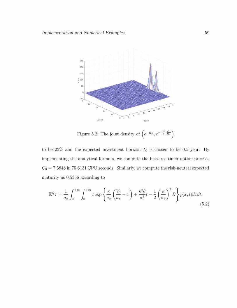
Implementation and Numerical Examples 59
00.1
0.20.3
0.40.5
0.60.7
0.80.9
1
0
0.2
0.4
0.6
0.8
1−50
0
50
100
150
200
250
z(t)−axisu(x)−axis
f−a
xis
Figure 5.2: The joint density of(e−RB , e−
∫ B
0duRu
)
to be 23% and the expected investment horizon T0 is chosen to be 0.5 year. By
implementing the analytical formula, we compute the bias-free timer option price as
C0 = 7.5848 in 75.6131 CPU seconds. Similarly, we compute the risk-neutral expected
maturity as 0.5356 according to
EQτ =1
σv
∫ +∞
0
∫ +∞
0
t exp
κ
σv
(V0
σv− x
)+
κ2θ
σ3v
t − 1
2
(κ
σv
)2
B
p(x, t)dxdt.
(5.2)

Implementation and Numerical Examples 60
Model and Option ParametersStock Price S0 100Option Strike K 100Variance Budget B 0.0265Correlation ρ -0.5000Initial Variance V0 0.0625Volatility of the Variance σv 0.1000Rate of Mean Reverting κ 2.0000Long Run Variance θ 0.0324Instantaneous Interest Rate r 0.04
Table 5.1: Model and Option Parameters
5.2 ADI Implementation of the PDE with Dimen-
sion Reduction
To begin with, we recall that the original PDE governing the timer option pricing
function u(t, s, v, x) is
∂u
∂t+κ(θ− v)
∂u
∂v+ rs
∂u
∂s+ v
∂u
∂x+
1
2σ2
vv∂2u
∂v2+
1
2s2v
∂2u
∂s2+ρσvsv
∂2u
∂s∂v− ru = 0, (5.3)
for (t, s, v, x) ∈ [0, +∞) × [0, +∞) × (0, +∞) × (0, B]. Given an arbitrary variance
budget, the timer option price u(t, s, v, x) is essentially independent of the initial time
t. In other words, timer options are perpetual. Therefore, we have that
∂u
∂t= 0.
This simplifies the original parabolic PDE (2.26) for pricing timer option to an elliptic
equation. Considering a boundary condition on plane:
Γ = (ξ1, ξ2, B), ξ1 ∈ R, ξ2 ∈ R,
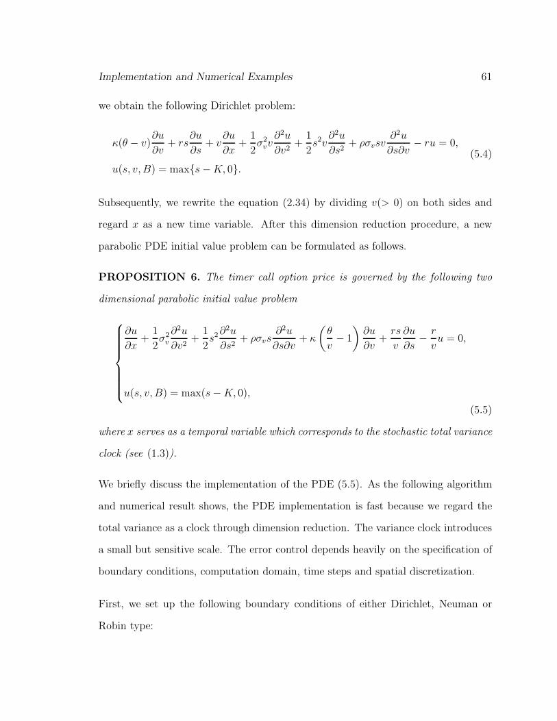
Implementation and Numerical Examples 61
we obtain the following Dirichlet problem:
κ(θ − v)∂u
∂v+ rs
∂u
∂s+ v
∂u
∂x+
1
2σ2
vv∂2u
∂v2+
1
2s2v
∂2u
∂s2+ ρσvsv
∂2u
∂s∂v− ru = 0,
u(s, v, B) = maxs − K, 0.(5.4)
Subsequently, we rewrite the equation (2.34) by dividing v(> 0) on both sides and
regard x as a new time variable. After this dimension reduction procedure, a new
parabolic PDE initial value problem can be formulated as follows.
PROPOSITION 6. The timer call option price is governed by the following two
dimensional parabolic initial value problem
∂u
∂x+
1
2σ2
v
∂2u
∂v2+
1
2s2∂2u
∂s2+ ρσvs
∂2u
∂s∂v+ κ
(θ
v− 1
)∂u
∂v+
rs
v
∂u
∂s− r
vu = 0,
u(s, v, B) = max(s − K, 0),
(5.5)
where x serves as a temporal variable which corresponds to the stochastic total variance
clock (see (1.3)).
We briefly discuss the implementation of the PDE (5.5). As the following algorithm
and numerical result shows, the PDE implementation is fast because we regard the
total variance as a clock through dimension reduction. The variance clock introduces
a small but sensitive scale. The error control depends heavily on the specification of
boundary conditions, computation domain, time steps and spatial discretization.
First, we set up the following boundary conditions of either Dirichlet, Neuman or
Robin type:
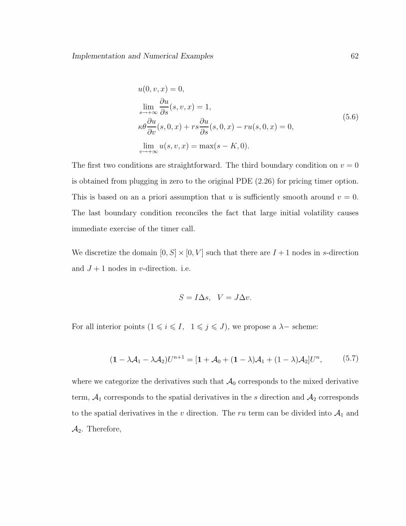
Implementation and Numerical Examples 62
u(0, v, x) = 0,
lims→+∞
∂u
∂s(s, v, x) = 1,
κθ∂u
∂v(s, 0, x) + rs
∂u
∂s(s, 0, x) − ru(s, 0, x) = 0,
limv→+∞
u(s, v, x) = max(s − K, 0).
(5.6)
The first two conditions are straightforward. The third boundary condition on v = 0
is obtained from plugging in zero to the original PDE (2.26) for pricing timer option.
This is based on an a priori assumption that u is sufficiently smooth around v = 0.
The last boundary condition reconciles the fact that large initial volatility causes
immediate exercise of the timer call.
We discretize the domain [0, S]× [0, V ] such that there are I + 1 nodes in s-direction
and J + 1 nodes in v-direction. i.e.
S = I∆s, V = J∆v.
For all interior points (1 6 i 6 I, 1 6 j 6 J), we propose a λ− scheme:
(1 − λA1 − λA2)Un+1 = [1 + A0 + (1 − λ)A1 + (1 − λ)A2]U
n, (5.7)
where we categorize the derivatives such that A0 corresponds to the mixed derivative
term, A1 corresponds to the spatial derivatives in the s direction and A2 corresponds
to the spatial derivatives in the v direction. The ru term can be divided into A1 and
A2. Therefore,
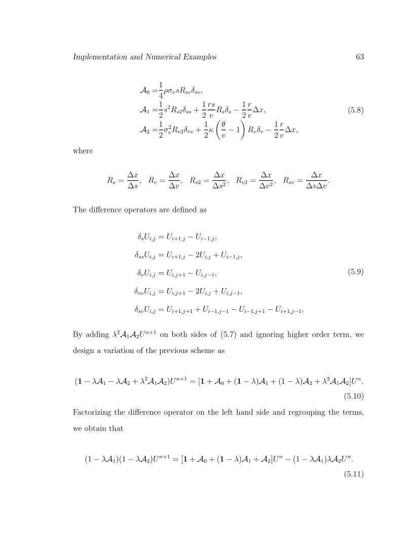
Implementation and Numerical Examples 63
A0 =1
4ρσvsRsvδsv,
A1 =1
2s2Rs2δss +
1
2
rs
vRsδs −
1
2
r
v∆x,
A2 =1
2σ2
vRv2δvv +1
2κ
(θ
v− 1
)Rvδv −
1
2
r
v∆x,
(5.8)
where
Rs =∆x
∆s, Rv =
∆x
∆v, Rs2 =
∆x
∆s2, Rv2 =
∆x
∆v2, Rsv =
∆x
∆s∆v.
The difference operators are defined as
δsUi,j = Ui+1,j − Ui−1,j ,
δssUi,j = Ui+1,j − 2Ui,j + Ui−1,j ,
δvUi,j = Ui,j+1 − Ui,j−1,
δvvUi,j = Ui,j+1 − 2Ui,j + Ui,j−1,
δsvUi,j = Ui+1,j+1 + Ui−1,j−1 − Ui−1,j+1 − Ui+1,j−1,
(5.9)
By adding λ2A1A2Un+1 on both sides of (5.7) and ignoring higher order term, we
design a variation of the previous scheme as
(1 − λA1 − λA2 + λ2A1A2)Un+1 = [1 + A0 + (1 − λ)A1 + (1 − λ)A2 + λ2A1A2]U
n.
(5.10)
Factorizing the difference operator on the left hand side and regrouping the terms,
we obtain that
(1 − λA1)(1 − λA2)Un+1 = [1 + A0 + (1 − λ)A1 + A2]U
n − (1 − λA1)λA2Un.
(5.11)
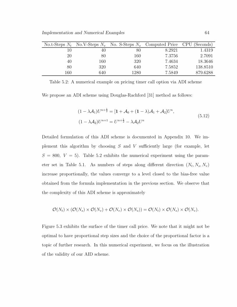
Implementation and Numerical Examples 64
No.t-Steps Nt No.V-Steps Nv No. S-Steps Ns Computed Price CPU (Seconds)10 40 80 8.2921 1.431920 80 160 7.3756 2.709140 160 320 7.4634 18.364680 320 640 7.5852 138.8510
160 640 1280 7.5849 879.6288
Table 5.2: A numerical example on pricing timer call option via ADI scheme
We propose an ADI scheme using Douglas-Rachford [31] method as follows:
(1 − λA1)Un+ 1
2 = [1 + A0 + (1 − λ)A1 + A2]Un,
(1 − λA2)Un+1 = Un+ 1
2 − λA2Un
(5.12)
Detailed formulation of this ADI scheme is documented in Appendix 10. We im-
plement this algorithm by choosing S and V sufficiently large (for example, let
S = 800, V = 5). Table 5.2 exhibits the numerical experiment using the param-
eter set in Table 5.1. As numbers of steps along different direction (Nt, Ns, Nv)
increase proportionally, the values converge to a level closed to the bias-free value
obtained from the formula implementation in the previous section. We observe that
the complexity of this ADI scheme is approximately
O(Nt) × (O(Ns) ×O(Nv) + O(Nv) ×O(Ns)) = O(Nt) ×O(Ns) ×O(Nv).
Figure 5.3 exhibits the surface of the timer call price. We note that it might not be
optimal to have proportional step sizes and the choice of the proportional factor is a
topic of further research. In this numerical experiment, we focus on the illustration
of the validity of our AID scheme.

Implementation and Numerical Examples 65
020
4060
80100
120140
160180
200
0
0.02
0.04
0.06
0.08
0.10
50
100
150
asset pricecurrent variance
timer
cal
l pric
e
(a) Timer call option price Surface
Figure 5.3: Timer call surfaces implemented from PDE ADI scheme
5.3 Monte Carlo Simulation
In this section, we propose two Monte Carlo simulation schemes and compare their
implementation with the PDE and the analytical formula. Algorithm 1 is a relatively
brute force method. Compared to using the discounted payoff e−rτ maxSτ − K, 0
as the estimator directly, Proposition 3 offers a conditional Monte Carlo simulation
estimator, which achieves the variance reduction. To further enhance the efficiency, we
employ the discounted asset price e−rτSτ as a control variate. (τ, Vτ ) is approximated
via a “time-checking” algorithm based on the exact simulation of the variance path
Vt. We notice that Algorithm 1 also works, when the Feller condition 2κθ−σ2v ≥ 0
is violated. As we can see in Appendix 10, Algorithm 1 can be adapted to incorporate
the consideration of jump risk. Algorithm 2 is an enhanced implementation based on
Proposition 4. Instead of manipulating the original variance process Vt, we employ
an Euler scheme on the Bessel process with predictor and corrector, which is applied
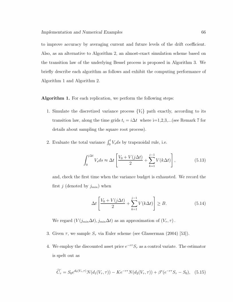
Implementation and Numerical Examples 66
to improve accuracy by averaging current and future levels of the drift coefficient.
Also, as an alternative to Algorithm 2, an almost-exact simulation scheme based on
the transition law of the underlying Bessel process is proposed in Algorithm 3. We
briefly describe each algorithm as follows and exhibit the computing performance of
Algorithm 1 and Algorithm 2.
Algorithm 1. For each replication, we perform the following steps:
1. Simulate the discretized variance process Vt path exactly, according to its
transition law, along the time grids ti = i∆t where i=1,2,3,...(see Remark 7 for
details about sampling the square root process).
2. Evaluate the total variance∫ t
0Vsds by trapezoidal rule, i.e.
∫ j∆t
0
Vsds ≈ ∆t
[V0 + V (j∆t)
2+
j−1∑
k=1
V (k∆t)
], (5.13)
and, check the first time when the variance budget is exhausted. We record the
first j (denoted by jmin) when
∆t
[V0 + V (j∆t)
2+
j−1∑
k=1
V (k∆t)
]≥ B. (5.14)
We regard (V (jmin∆t), jmin∆t) as an approximation of (Vτ , τ) .
3. Given τ , we sample Sτ via Euler scheme (see Glasserman (2004) [53]).
4. We employ the discounted asset price e−rτSτ as a control variate. The estimator
is spelt out as
Cτ = S0ed0(Vτ ,τ)N(d1(Vτ , τ)) − Ke−rτN(d2(Vτ , τ)) + β∗(e−rτSτ − S0), (5.15)

Implementation and Numerical Examples 67
where the optimal coefficient β∗ is the opposite number of the slope of the least-
square regression line of the samples of S0ed0(Vτ ,τ)N(d1(Vτ , τ))−Ke−rτN(d2(Vτ , τ))
against that of e−rτSτ . We use the sample version to estimate β∗ in the im-
plementation, i.e. use the ratio of the covariance of the two statistics and the
variance of the control variable.
REMARK 7. By Cox et al. [25], the distribution of Vt given Vu where u < t, up to
a scale factor, is a noncentral chi-squared distribution, i.e.
Vt =σ2
v(1 − e−κ(t−u))
4κχ′2
d
(4κe−κ(t−u)
σ2v(1 − e−κ(t−u))
Vu
), for t > u,
where χ′2d denotes the noncentral chi-squared random variable with d degrees of free-
dom, non-centrality parameter λ and d = 4θκσ2
v. See Broadie and Kaya [17] for detailed
study about the exact simulation of process Vt.
Algorithm 2 relies on the representation of timer call option price via Bessel processes
in Proposition 4. Here we propose an Euler scheme with Predictor-Corrector on the
Bessel SDE. We apply the Brownian scaling property to derive the following property,
in order to recast the variance budget B as a model parameter.
COROLLARY 4. Let Yt, Zt be a bivariate diffusion process governed by stochas-
tic differential equation:
dYt = Bκ · θ
Ytdt + σv
√Bdβt; Y0 = V0,
dZt =B
Ytdt; Z0 = 0,
(5.16)
where βt is a standard Brownian motion. Under probability measure P0, the fol-

Implementation and Numerical Examples 68
lowing distributional identity holds,
(σvXB,
∫ B
0
ds
σvXs
)≡law (Y1, Z1).
Thus, the algorithm can be described as follows.
Algorithm 2. For each replication, we perform an Euler iteration with predictor and
corrector (see Jaeckel [63]) in order to compensate the error caused by the unattain-
able zero pole of Bessel processes. Numerical experiments shows that this algorithm
works very well.
1. Predictor:
Y (i + 1) = Y (i) +Bκθ
Y (i)∆t + σv
√B√
∆tβ(i), Y (0) = V0,
2. Corrector:
Y (i + 1) = Y (i) +
[αBκθ
Y (i + 1)+
(1 − α)Bκθ
Y (i)
]∆t + σv
√B√
∆tβ(i),
Y (0) = V0, where β(i)’s are standard normal random variables; α is an adjusting
coefficient which is usually chosen as 12.
3.
Z(i + 1) = Z(i) +1
2∆tB
[1
Y (i)+
1
Y (i + 1)
], Z(0) = 0.
According to Proposition 4, the estimator is Ψ(Y1, Z1).
As an alternative to Algorithm 2, an almost-exact simulation based on the transition
law of the underlying Bessel process is proposed as follows. We start with the following
lemma about the transition law of Bessel processes (see Delbaen and Shirakawa [28]).
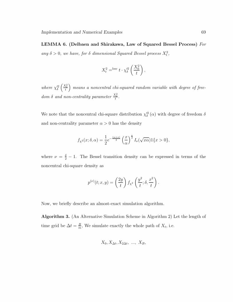
Implementation and Numerical Examples 69
LEMMA 6. (Delbaen and Shirakawa, Law of Squared Bessel Process) For
any δ > 0, we have, for δ dimensional Squared Bessel process X2t ,
X2t =law t · χ′2
δ
(X2
0
t
),
where χ′2δ
(X2
0
t
)means a noncentral chi-squared random variable with degree of free-
dom δ and non-centrality parameterX2
0
t.
We note that the noncentral chi-square distribution χ′2δ (α) with degree of freedom δ
and non-centrality parameter α > 0 has the density
fχ2(x; δ, α) =1
2e−
(α+x)2
(x
α
) ν2Iν(
√xα)1x > 0,
where ν = δ2− 1. The Bessel transition density can be expressed in terms of the
noncentral chi-square density as
p(ν)(t; x, y) =
(2y
t
)fχ2
(y2
t; δ,
x2
t
).
Now, we briefly describe an almost-exact simulation algorithm.
Algorithm 3. (An Alternative Simulation Scheme in Algorithm 2) Let the length of
time grid be ∆t = Bm
, We simulate exactly the whole path of Xt, i.e.
X0, X∆t, X2∆t, ..., XB,
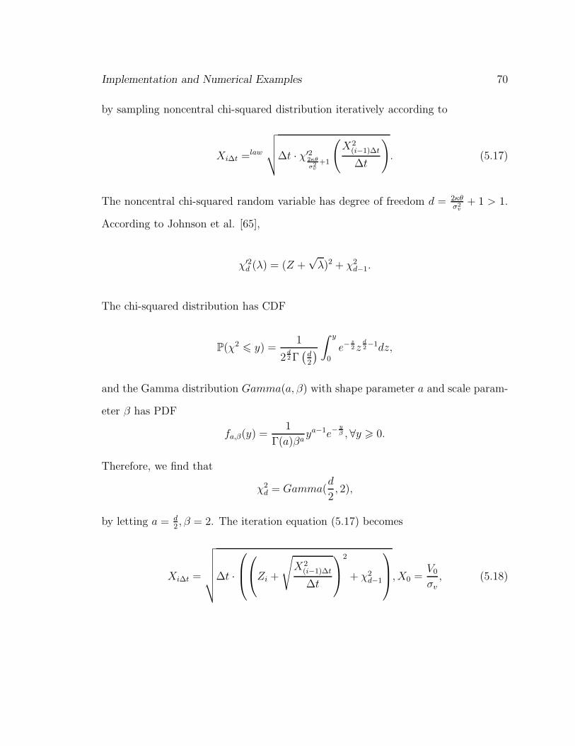
Implementation and Numerical Examples 70
by sampling noncentral chi-squared distribution iteratively according to
Xi∆t =law
√√√√∆t · χ′22κθ
σ2v
+1
(X2
(i−1)∆t
∆t
). (5.17)
The noncentral chi-squared random variable has degree of freedom d = 2κθσ2
v+ 1 > 1.
According to Johnson et al. [65],
χ′2d (λ) = (Z +
√λ)2 + χ2
d−1.
The chi-squared distribution has CDF
P(χ2 6 y) =1
2d2 Γ(
d2
)∫ y
0
e−z2 z
d2−1dz,
and the Gamma distribution Gamma(a, β) with shape parameter a and scale param-
eter β has PDF
fa,β(y) =1
Γ(a)βaya−1e−
yβ , ∀y > 0.
Therefore, we find that
χ2d = Gamma(
d
2, 2),
by letting a = d2, β = 2. The iteration equation (5.17) becomes
Xi∆t =
√√√√√√∆t ·
Zi +
√X2
(i−1)∆t
∆t
2
+ χ2d−1
, X0 =
V0
σv, (5.18)

Implementation and Numerical Examples 71
where d = 2κθσ2
v+ 1 and
χ2d−1 = χ2
2κθ
σ2v
= Gamma
(κθ
σ2v
, 2
)= 2Gamma
(κθ
σ2v
, 1
),
where the shape parameter of the Gamma variables is κθσ2
v. To sample Gamma vari-
ables, we use Fishman’s algorithm (see Fishman [42]).
Thus, we can sample Vτ through σvXB = σvXm∆t. We use trapezoidal rule to ap-
proximate τ as 1Xt
τ =
∫ B
0
ds
σvX(s)≈ 1
2
m∑
i=1
1
σv
(1
X i−1m
B
+1
X im
B
)B
m.
According to Duffie and Glynn [34], it is asymptotically optimal to increase the num-
ber of time steps proportional to the square root of the number of simulation trials
for the first order Euler discretization. For Algorithm 1, we suppose the number of
simulation trials is n and number of time steps for going from 0 to T0 (the speci-
fied investment horizon) is k. Thus we apply the optimality principle in Duffie and
Glynn [34] in the sense that k = [√
n] (∆t = T0/k). Table 5.3 and Figure 5.4 shows
our implementation results. It is obvious that Algorithm 2 significantly outperforms
Algorithm 1.
5.4 Miscellaneous Features
Finally, we illustrate the comparison between timer call options and European call
options with the same expected investment horizon (maturity) by a numerical ex-
ample. Indeed, we specify an investment horizon, e.g. T0 = 0.25. Using the model
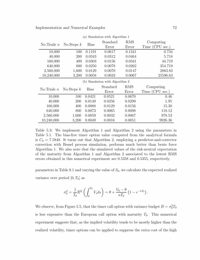
Implementation and Numerical Examples 72
(a) Simulation with Algorithm 1
No.Trials n No.Steps k BiasStandard
ErrorRMSError
ComputingTime (CPU sec.)
10,000 100 0.1191 0.0617 0.1341 0.73440,000 200 0.0343 0.0312 0.0464 5.718
160,000 400 0.0303 0.0156 0.0341 44.719640,000 800 0.0250 0.0078 0.0262 354.719
2,560,000 1,600 0.0129 0.0070 0.0147 2863.8310,240,000 3,200 0.0058 0.0033 0.0067 25596.63
(b) Simulation with Algorithm 2
No.Trials n No.Steps k BiasStandard
ErrorRMSError
ComputingTime (CPU sec.)
10,000 100 0.0421 0.0521 0.0670 0.4640,000 200 0.0149 0.0256 0.0299 1.95
160,000 400 0.0088 0.0129 0.0156 15.38640,000 800 0.0073 0.0065 0.0098 118.12
2,560,000 1,600 0.0059 0.0032 0.0067 978.5310,240,000 3,200 0.0049 0.0016 0.0051 9926.36
Table 5.3: We implement Algorithm 1 and Algorithm 2 using the parameters inTable 5.1. The bias-free timer option value computed from the analytical formulais C0 = 7.5848. It turns out that Algorithm 2, employing a predictor-and-correctorcorrection with Bessel process simulation, performs much better than brute forceAlgorithm 1. We also note that the simulated values of the risk-neutral expectationof the maturity from Algorithm 1 and Algorithm 2 associated to the lowest RMSerrors obtained in this numerical experiment are 0.5358 and 0.5355, respectively.
parameters in Table 9.1 and varying the value of S0, we calculate the expected realized
variance over period [0, T0] as
σ20 =
1
T0
EQ
(∫ T0
0
Vsds
)= θ +
V0 − θ
κT0
(1 − e−κT0
).
We observe, from Figure 5.5, that the timer call option with variance budget B = σ20T0
is less expensive than the European call option with maturity T0. This numerical
experiment suggests that, as the implied volatility tends to be mostly higher than the
realized volatility, timer options can be applied to suppress the extra cost of the high
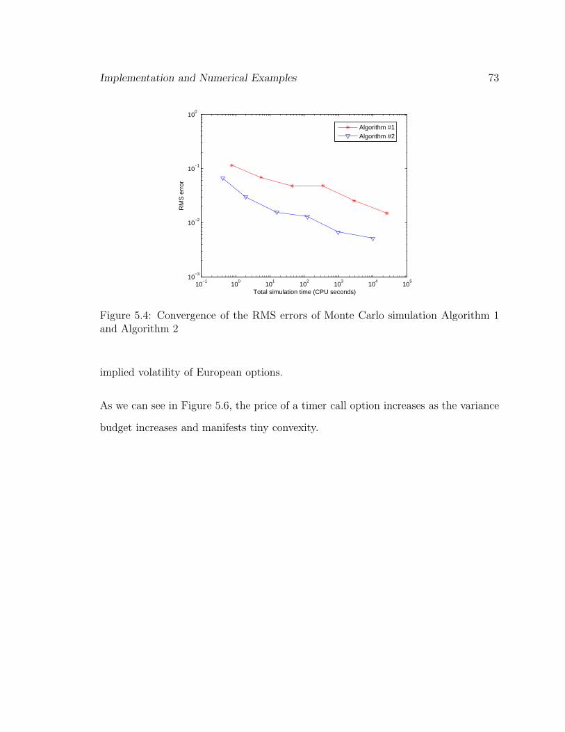
Implementation and Numerical Examples 73
10−1
100
101
102
103
104
105
10−3
10−2
10−1
100
Total simulation time (CPU seconds)
RM
S e
rror
Algorithm #1Algorithm #2
Figure 5.4: Convergence of the RMS errors of Monte Carlo simulation Algorithm 1and Algorithm 2
implied volatility of European options.
As we can see in Figure 5.6, the price of a timer call option increases as the variance
budget increases and manifests tiny convexity.
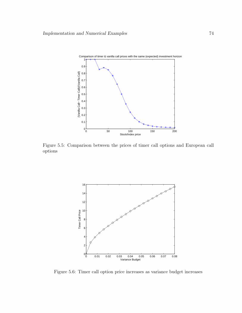
Implementation and Numerical Examples 74
0 50 100 150 2000
0.1
0.2
0.3
0.4
0.5
0.6
0.7
0.8
0.9
1
Stock/Index price
(Van
illa
Cal
l− T
imer
Cal
l)/(V
anill
a C
all)
Comparison of timer & vanilla call prices with the same (expected) investment horizon
Figure 5.5: Comparison between the prices of timer call options and European calloptions
0 0.01 0.02 0.03 0.04 0.05 0.06 0.07 0.080
2
4
6
8
10
12
14
16
Variance Budget
Tim
er C
all P
rice
Figure 5.6: Timer call option price increases as variance budget increases

Chapter 6
Dynamic Hedging Strategies
In this chapter, we discuss dynamic hedging strategies for timer options at the theoret-
ical level. We also briefly illustrate the issue of the computation of price sensitivities
used for hedging and risk-management purposes.
6.1 Dynamic Hedging Strategies
The underlying asset and the riskless money market account constitute an incom-
plete market due to the uncertain volatility risk. Thanks to the market completion
via volatility-dependent assets (e.g. variance swap), we formulate the pricing of timer
option as a first-passage-time problem via a standard no-arbitrage argument in Chap-
ter 2. In this chapter, we focus on the dynamic hedging (replication) of timer option
based on market completion.
We hedge the timer call option by the original underlying asset and a sequence of
contiguous auxiliary volatility-dependent securities. In the following exposition, we
take variance swap as an example of the auxiliary hedging instruments. Because we
75

Dynamic Hedging Strategies 76
need to hedge the timer call option until its random maturity τ , we may need to
replace matured variance swaps with new ones during the whole life of the timer
call option. We regard [0, τ ] as a composition of hedging periods Di = [∑i−1
j=0 Tj ∧
τ,∑i
j=0 Tj∧τ ], i = 1, 2, 3, ... (we define T0 = 0). On Di a variance swap with maturity
Ti and price process Gi(t) is employed as an auxiliary hedging instrument. In fact,
in order to hedge a timer option we need not only to rebalance the replicating portfolio
locally within each period Di, but we also need to replace the expired variance swap
with a new one at each time Ti, if Ti < τ , until time τ when the total variance budget
is consumed. The following chart illustrates this hedging mechanism.
C0
Π0 = C0
(∆St , ∆
G(1)t )
hedge−−−→
CT1
ΠT1= CT1
(∆St , ∆
G(2)t )
hedge−−−→ ... hedge−−−→
Cτ = max(Sτ − K, 0)
Πτ = Cτ
(∆St , ∆
G(n)t )
Without loss of generality, we focus on the first hedging period [0, T1 ∧ τ ]. Let Πt
denote the value process of the self-financing hedging portfolio. Suppose that at time
t the portfolio consists of ∆st shares of asset with price St and ∆G
t shares of variance
swap with price Gt (note that we drop the subscription 1 of G1 without introducing
any confusion), and the rest of the money fully invested in the riskless money market
account. Therefore,
dΠt = ∆St dSt + ∆G
t dGt + r(Πt − ∆St St − ∆G
t Gt)dt.
It is equivalent to
d(e−rtΠt) = e−rt[∆S
t (dSt − rStdt) + ∆Gt (dGt − rGtdt)
].
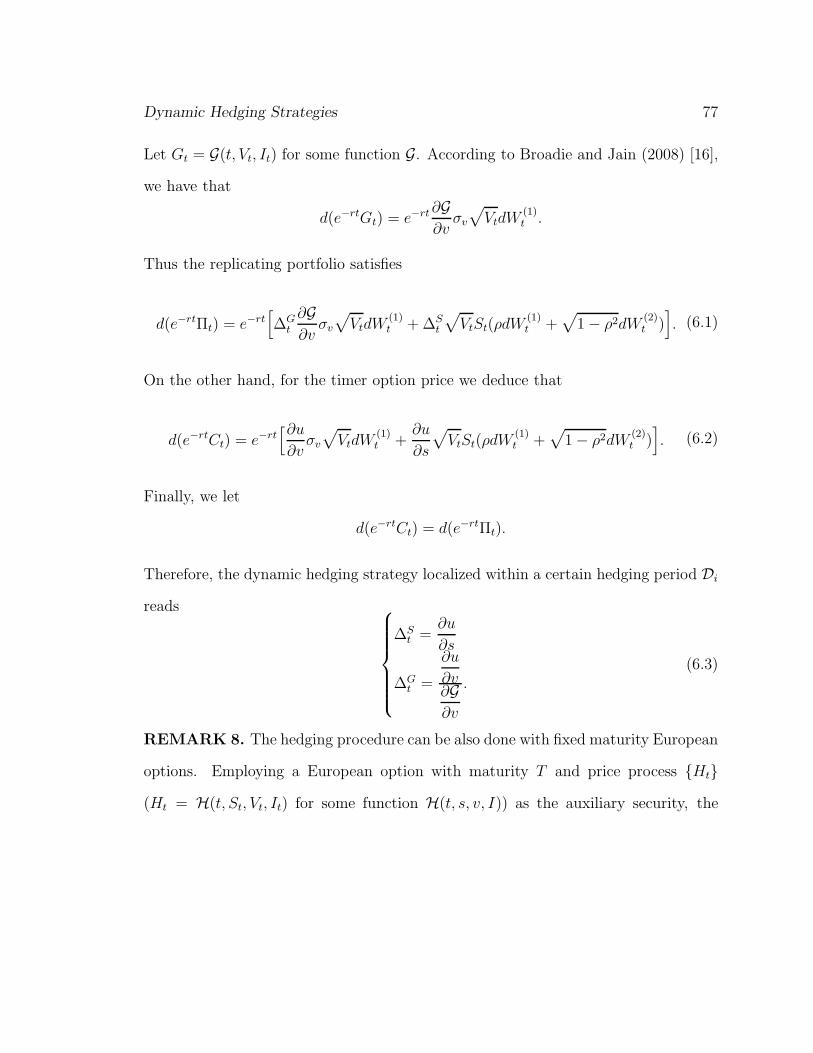
Dynamic Hedging Strategies 77
Let Gt = G(t, Vt, It) for some function G. According to Broadie and Jain (2008) [16],
we have that
d(e−rtGt) = e−rt ∂G∂v
σv
√VtdW
(1)t .
Thus the replicating portfolio satisfies
d(e−rtΠt) = e−rt[∆G
t
∂G∂v
σv
√VtdW
(1)t + ∆S
t
√VtSt(ρdW
(1)t +
√1 − ρ2dW
(2)t )]. (6.1)
On the other hand, for the timer option price we deduce that
d(e−rtCt) = e−rt[∂u
∂vσv
√VtdW
(1)t +
∂u
∂s
√VtSt(ρdW
(1)t +
√1 − ρ2dW
(2)t )]. (6.2)
Finally, we let
d(e−rtCt) = d(e−rtΠt).
Therefore, the dynamic hedging strategy localized within a certain hedging period Di
reads
∆St =
∂u
∂s
∆Gt =
∂u
∂v∂G∂v
.(6.3)
REMARK 8. The hedging procedure can be also done with fixed maturity European
options. Employing a European option with maturity T and price process Ht
(Ht = H(t, St, Vt, It) for some function H(t, s, v, I)) as the auxiliary security, the

Dynamic Hedging Strategies 78
strategy for dynamically hedging a timer call option reads
∆St =
∂u
∂s−
∂u
∂v· ∂H
∂s∂H∂v
∆Ht =
∂u
∂v∂H∂v
.
(6.4)
6.2 Computation of Price Sensitivities
From Section 6.1, we see that both timer call Delta (the sensitivity with respect to
S0) and Vega (the sensitivity with respect to V0) are important for dynamic hedging
of timer options. Price sensitivities on other model parameters might be useful for
risk management purpose. In this section, we discuss the computation of sensitivities
based on various computational methods we discussed previously.
Upon implementing the analytical formula in Theorem 4, we can use the correspond-
ing finite difference to approximate a sensitivity. For a general parameter Θ (could
be S0,V0, etc)
∂C0
∂Θ≈ C0(Θ + δΘ) − C0(Θ)
δΘ.
It is straightforward to implement it by choosing small δΘ so as to achieve a pre-
specified error tolerance level. We can also perform path-wise simulation (see Broadie
and Glasserman [15]) to compute price sensitivities. We can obtain the sensitivities
almost for free, once the simulation of underlying process is done for valuation. How-
ever, we need to tolerate the bias in this approach. Based on Proposition 4 and
Corollary (5.16), we can apply pathwise approach combined with Euler discretiza-
tion on the Bessel process in order to compute the price sensitivities with respect to
Θ ∈ B, κ, θ, σv, V0. By taking the derivatives inside the expectation, we obtain the
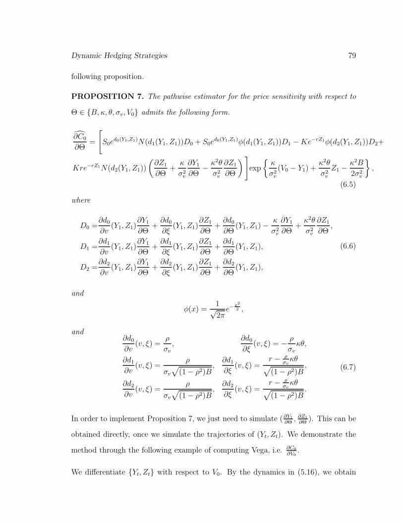
Dynamic Hedging Strategies 79
following proposition.
PROPOSITION 7. The pathwise estimator for the price sensitivity with respect to
Θ ∈ B, κ, θ, σv, V0 admits the following form.
∂C0
∂Θ=
[S0e
d0(Y1,Z1)N(d1(Y1, Z1))D0 + S0ed0(Y1,Z1)φ(d1(Y1, Z1))D1 − Ke−rZ1φ(d2(Y1, Z1))D2+
Kre−rZ1N(d2(Y1, Z1))
(∂Z1
∂Θ+
κ
σ2v
∂Y1
∂Θ− κ2θ
σ2v
∂Z1
∂Θ
)]exp
κ
σ2v
(V0 − Y1) +κ2θ
σ2v
Z1 −κ2B
2σ2v
,
(6.5)
where
D0 =∂d0
∂v(Y1, Z1)
∂Y1
∂Θ+
∂d0
∂ξ(Y1, Z1)
∂Z1
∂Θ+
∂d0
∂Θ(Y1, Z1) −
κ
σ2v
∂Y1
∂Θ+
κ2θ
σ2v
∂Z1
∂Θ,
D1 =∂d1
∂v(Y1, Z1)
∂Y1
∂Θ+
∂d1
∂ξ(Y1, Z1)
∂Z1
∂Θ+
∂d1
∂Θ(Y1, Z1),
D2 =∂d2
∂v(Y1, Z1)
∂Y1
∂Θ+
∂d2
∂ξ(Y1, Z1)
∂Z1
∂Θ+
∂d2
∂Θ(Y1, Z1),
(6.6)
and
φ(x) =1√2π
e−x2
2 ,
and∂d0
∂v(v, ξ) =
ρ
σv
,∂d0
∂ξ(v, ξ) = − ρ
σv
κθ,
∂d1
∂v(v, ξ) =
ρ
σv
√(1 − ρ2)B
,∂d1
∂ξ(v, ξ) =
r − ρσv
κθ√
(1 − ρ2)B,
∂d2
∂v(v, ξ) =
ρ
σv
√(1 − ρ2)B
,∂d2
∂ξ(v, ξ) =
r − ρσv
κθ√
(1 − ρ2)B.
(6.7)
In order to implement Proposition 7, we just need to simulate (∂Y1
∂Θ, ∂Z1
∂Θ). This can be
obtained directly, once we simulate the trajectories of (Yt, Zt). We demonstrate the
method through the following example of computing Vega, i.e. ∂C0
∂V0.
We differentiate Yt, Zt with respect to V0. By the dynamics in (5.16), we obtain

Dynamic Hedging Strategies 80
that,
d
(∂Yt
∂V0
)= − Bκθ
Y 2t
(∂Yt
∂V0
)dt;
∂Y0
∂V0= 1,
d
(∂Zt
∂V0
)= − B
Y 2t
(∂Yt
∂V0
)dt;
∂Z0
∂V0= 0.
(6.8)
Therefore, by discretization, we design the following Euler scheme to simulate (∂Y1
∂V0, ∂Z1
∂V0).
(∂Y
∂V0
)(i + 1) =
(∂Y
∂V0
)(i) − Bκθ
Y 2(i)
(∂Y
∂V0
)(i)∆t,
(∂Z
∂V0
)(i + 1) =
(∂Z
∂V0
)(i) − B
Y 2(i)
(∂Y
∂V0
)(i)∆t.
(6.9)
We take the terminal value from these iterations to evaluate the estimators for the
price sensitivities.
As to the computation of sensitivities via PDE approach, we use finite difference to
approximate the corresponding derivatives. It is straightforward to obtain the price
sensitivity with respect to S0 (the so called Delta) and the price sensitivity with
respect to V0 (the so called Vega) once the price surface 6.1 is obtained.
For the purpose of illustration, we plot the surface of timer call Delta and Vega,
which are both important for hedging, in Figure 6.1. We observe that the Delta of
the timer call option is bounded between zero and one, while the Vega keeps negative
with considerable fluctuation.

Dynamic Hedging Strategies 81
020
4060
80100
120140
160180
200
0
0.02
0.04
0.06
0.08
0.10
0.2
0.4
0.6
0.8
1
1.2
1.4
asset pricecurrent variance
price
se
nsi
tivity
wrt
S (
De
lta)
(a) Timer call Delta ∂C
∂S0
0
50
100
150
2000 0.01 0.02 0.03 0.04 0.05 0.06 0.07 0.08 0.09 0.1
−90
−80
−70
−60
−50
−40
−30
−20
−10
0
10
current varianceasset price
Ve
ga
(b) Timer call Vega ∂C
∂V0
Figure 6.1: Numerical examples of time call option price sensitivities: Delta and Vega

Part II
Efficient Valuation of VIX Options
under Gatheral’s Double
Log-normal Stochastic Volatility
Model
82

Chapter 7
Introduction to Part II
7.1 A Brief Outline of Part II
Consistent modeling and pricing of options on S&P 500 (the Standard and Poor’s
500 index), VIX (the CBOE volatility index) and realized variance are an important
issues for the financial derivatives market. Gatheral’s (2007, 2008) double mean-
reverting stochastic volatility model achieves such a goal to reduce the model risk.
However, the non-affine structure of this model leads to the analytical intractability in
the sense that the characteristic function of the underlying variables might not exist
in closed-form. At the time when the model was proposed, its calibration involved
massive Monte Carlo simulation. In this part, we begin with some analysis of the
model. Then, we develop a generally applicable asymptotic expansion method for
efficient valuation of derivatives under non-affine multidimensional diffusion models;
and demonstrate it in the valuation of options on VIX under Gatheral’s double log-
normal model. Our probabilistic method is a combination of scaling, pathwise Tay-
83

Introduction to Part II 84
lor expansion, inductive computation of correction terms, calculation of conditional
mixed Brownian moments, etc. The non-linear payoff function of an option on VIX
is complicated; nevertheless convergence of our expansion is rigorously justified via
the theory of Malliavin-Watanabe-Yoshida. In numerical examples, we demonstrate
that the formula efficiently achieves desirable accuracy for relatively short maturity
cases. Following our probabilistic computation approach and theoretical basis, bet-
ter accuracy for longer maturity options can be obtained by adding more correction
terms.
7.2 Modeling VIX
VIX, the Chicago Board Options Exchange (CBOE) Volatility Index (see [23]), is the
premier benchmark for U.S. stock market volatility. It provides investors a direct and
effective way to understand volatility. As an implied volatility index, VIX measures
market expectations of near term (next 30 calendar days) volatility conveyed by stock
index option prices. Since volatility often signifies financial turmoil, VIX is often
referred to as the “investor fear gauge”.
According to CBOE [23], independent of model specification, an index σ2 is calculated
by averaging the weighted prices of out-of-the-money puts and calls on S&P 500 (the
Standard & Poor’s 500 index), i.e.
σ2 =2
∆T
∑
i
∆Ki
K2i
er∆T Q(Ki) −1
∆T
[F
K0− 1
]2
, (7.1)
where the various parameters are defined as follows.

Introduction to Part II 85
∆T : Time to expiration,
F : Forward index level derived from index option prices,
Ki : Strike price of i-th out-of-the-money option,
∆Ki : Interval between strike prices,
K0 : First strike below the forward index level F ,
r : Risk-free interest rate to expiration,
Q(Ki) : The midpoint of the bid-ask spread for each option
with strike Ki.
Conventionally, VIX is calculated as
V IX = σ × 100. (7.2)
The squared VIX satisfies that
V IX2 =2 × 10⁴
T
∑
i
∆Ki
K2i
erT Q(Ki) −104
T
[F
K0− 1
]2
. (7.3)
Following Carr and Wu (2006) [22], we introduce the theoretical proxy of VIX and
demonstrate the necessity of employing a model, which is able to consistently price
options on VIX and S&P 500. To begin with, we recall the definition of theoretical
VIX, which is used in the modeling and valuation of derivative securities on VIX.
On the filtered risk neutral probability space (Ω, Q,F , Ft), we assume the asset
dynamics to be
dSt
St= rdt +
√VtdWt,
where Vt denotes the stochastic variance process. Let us define the realized variance
Introduction to Part II 86
over the time interval [t, t + ∆T ] to be
RVt,t+∆T :=1
∆T
∫ t+∆T
t
Vsds.
Further, V IX2
t , the theoretical squared VIX (see Carr and Wu [22]) is defined as
V IX2
t = EQ[RVt,t+∆T |Ft] = EQ
[1
∆T
∫ t+∆T
t
Vsds
∣∣∣∣∣Ft
]. (7.4)
For now, we exclude the presence of jump in the asset dynamics. Otherwise, jumps
will contribute to the realized variance as well. The theoretical squared VIX (7.4)
can be statically replicated via forward-starting S&P 500 put and call options, i.e.
V IX2
t =2
∆T
[∫ ∞
Ft
er∆T
K2CModel(t, t + ∆T, K)dK +
∫ Ft
0
er∆T
K2P Model(t, t + ∆T, K)dK
],
(7.5)
where Ft = Ster(T−t) denotes the forward price of St contracted for a later time T > t.
CModel(t, t+∆T, K) and P Model(t, t+∆T, K) denote the model price of forward started
call and put options with maturity ∆T , respectively. This static replication idea has
been successfully applied to the study of variance swaps (see Derman et al. [29]).
Thus, the theoretical squared VIX (7.4) is represented by a strip of model-generating
out-of-the-money S&P 500 option prices over a wide range of strikes.
Suppose that we have a stochastic volatility model which fits the entire S&P 500
Introduction to Part II 87
options smile. In other words, for any strike K,
CModel(t, t + ∆T, K) =e−r∆T EQt (St+∆T − K)+
=CBS(σimp(K, ∆T ), St) = CMarket(t, t + ∆T, K)
P Model(t, t + ∆T, K) =e−r∆T EQt (K − St+∆T )+
=PBS(σimp(K, ∆T ), St) = P Market(t, t + ∆T, K).
(7.6)
where CMarket(t, t + ∆T, K) and P Market(t, t + ∆T, K) denote the market price of
forward started call and put options with maturity T . Here CBS and PBS denote the
Black-Scholes call and put option pricing formulae, respectively; and σimp(K, ∆T )
denotes the implied volatility associated with strike K and maturity ∆T . Therefore,
it follows that
V IX2
t =2
∆T
[∫ ∞
Ft
er∆T
K2CMarket(t, t + ∆T, K)dK +
∫ Ft
0
er∆T
K2P Market(t, t + ∆T, K)dK
].
(7.7)
Hence, we can interpret σ (defined in (7.3)) as a discretization of its theoretical
counterpart defined in (7.4). i.e.
V IX2≈ σ2. (7.8)
Therefore, we have that
V IX × 100 ≈ V IX. (7.9)
An excellent stochastic volatility model, under which the approximate relation (7.8)
holds, allows us to use theoretical VIX (7.4) as a proxy to study the pricing of VIX
options and futures, etc. within a continuous time framework. Therefore, we need
a model which matches S&P 500 options market prices across all strikes and also

Introduction to Part II 88
produces correct VIX option market prices. Under the assumption of absence of
jumps in the asset dynamics, the error resulted from using theoretical VIX is solely
induced by the discretization of the integration in (7.7) on strikes.
Similar to the Black-Scholes-Merton model (1973) [10, 79] for pricing equity options,
Whaley’s (1993) [91] model directly regarded VIX as a geometric Brownian motion
with constant volatility. Following the modeling approach in Cox et al. (1985) [26]
and Heston (1993) [61], Grunbichler and Longstaff (1996) [55] specified the dynam-
ics of VIX as a mean-reverting square root process. Detemple and Osakwe (2000)
[30] employed a logarithmic mean-reverting process for pricing options on volatility.
Carr and Lee (2007) [20] (also see Carr and Wu (2006) [22]) proposed a model-free
approach by using the associated variance and volatility swap rates as the model in-
puts. Following Eraker et al. (2003, 2004) [40, 64], Lin and Chang (2009) modeled
the S&P 500 index and the S&P 500 stochastic volatility by correlated jump-diffusion
processes. Following the approach proposed in Bergomi (2005, 2009) [6, 7], Cont and
Kokholm (2009) studied a modeling framework for the joint dynamics of an index
and a set of forward varaince swap rates written on this index.
7.3 Historical Developments on Modeling Multi-
factor Stochastic Volatility
The Black-Scholes-Merton (1973) model [10, 79] assumes that the underlying volatil-
ity is constant over the life of the derivative, and is unaffected by the changes in
the underlying asset price. However, one of the most prominent shortcomings of
this model is that it cannot explain features of the implied volatility surface such
as volatility smile and skew, which indicate that implied volatility does tend to vary
Introduction to Part II 89
with respect to strike price and expiration. Stochastic volatility is a popular approach
to resolve such deficiency of the Black-Scholes-Merton (1973) model. In particular,
the early attempts of two-factor stochastic volatility models, such as Hull and White
(1987) [62] and Heston (1993) [61], assume that the volatility of the underlying price is
a stochastic process rather than a constant, which makes it possible to model deriva-
tives more accurately. Two-factor stochastic volatility models can fit the volatility
smiles. However, these models are restrictive in the modeling of the relationship be-
tween the S&P 500 volatility level and the slope of the smile. The consistent modeling
of options on VIX and realized variance is confronted with even more challenge.
In the literature of equity/index option valuation, the deficiencies of the two-factor
stochastic volatility model have traditionally been addressed by adding jump compo-
nents to the dynamics. See for example Bates (1996) [4], Duffie, Pan and Singleton
(2000) [36], Broadie, Chernov and Johannes (2007) [14] and Lipton (2002) [75]. We do
not doubt the usefulness of this approach. Instead, we claim that adding additional
factors to the volatility process can alternatively circumvent the model deficiencies.
Here, we do not investigate whether multi-factor models or jump processes are more
appropriate for modeling option data.
Early considerations of using multi-factor stochastic volatility models to improve the
goodness of fit for S&P 500 returns can be found in Bates (1997) [5] and Gallant et.
al (1999) [47]. Duffie, Pan and Singleton (2000) [36] propose an affine class ∗ of three-
factor stochastic volatility models. Based on an assumption on the specific correlation
structure, an intermediate stochastic trend component is added to volatility, which
generalizes Heston’s (1993) [61] two-factor stochastic volatility model. Also relying on
the affine class, Heston et al. (2009) [24] propose a three-factor stochastic volatility
∗For the affine class models, see Duffie and Kan (1996) [35], Duffie, Filipovic and Schachermayer(2003) [33].
Introduction to Part II 90
model by adding a second CIR process of variance, which is independent of the one
in Heston (1993) [61]. Due to the special requirement on the correlation structure,
this model is analytically tractable in the sense that the characteristic function of the
underlying admits closed-form formula.
Gatheral’s double mean-reverting stochastic volatility model (2007, 2008) [50, 49, 51]
generalizes the affine three-factor model in Duffie, Pan and Singleton (2000) [36] by
allowing more flexibility in the correlation structure and the specification of the diffu-
sion components. Supported by some empirical study, the variance is more properly
modeled by a double-CEV type mean-reverting process instead of using square root
processes. Thus, it falls into the non-affine class, which is quite computationally
challenging.
7.4 Gatheral’s Double Mean-Reverting Stochastic
Volatility Model
Under the risk-neutral probability measure, Gatheral’s double mean-reverting stochas-
tic volatility model (hereafter DMR-SV) is specified as follows:
dSt
St=rdt +
√VtdW (t), S0 = s0 > 0,
dVt =κ(V ′t − Vt)dt + ξ1V
αt dZ1(t), V0 = v0 > 0,
dV ′t =c(z3 − V ′
t )dt + ξ2V′βt dZ2(t), V ′
0 = v′0 > 0,
(7.10)
where the Brownian motions are correlated as
dZ1(t)dZ2(t) = ρdt, dW (t)dZ1(t) = ρ1dt, dW (t)dZ2(t) = ρ2dt. (7.11)
Introduction to Part II 91
This model is presented in Gatheral (2007) [49], its further development in Gatheral
(2008a) [51] and Gatheral (2008b) [50]. In this model, St represents the price
process of a stock or index. The instantaneous variance level Vt reverts to the moving
intermediate level V ′t at rate k, while V ′
t reverts to the long-term level z3 at the
slower rate c < k. In the dynamics (7.10), r is the instantaneous interest rate, which
is assumed to be a constant; ξ1 and ξ2 are the volatility parameter for Vt and
V ′t , respectively; α and β are the constant elasticity parameters for Vt and V ′
t ,
respectively. By adding such a moving intermediate level, an additional freedom is
given compared to traditional two-factor stochastic volatility models, e.g. Heston
(1993) [61], etc. It provides a new perspective, from financial economics, for us to
capture more about the dynamics of stochastic volatility. In this dissertation, we
focus on the study of the double mean-reverting volatility process (Vt, V′t ).
The CEV (constant elasticity of volatility) type parameters are chosen as α, β ∈
[1/2, 1]. According to Gatheral [50], the models are classified as:
• Double Heston for the case of α = β = 1/2,
• Double Log-normal for the case α = β = 1,
• Double CEV for any other cases.
We note that both Vt and V ′t are always finite and positive. For the case of double
log-normal (α = β = 1), this property of (Vt, V′t ) can be seen from its explicit solution.
PROPOSITION 8. When α = β = 1, the linear stochastic differential equation
Introduction to Part II 92
governing the bivariate diffusion (Vt, V′t ) can be solved explicitly as
V ′(t) = exp
−ct + ξ2B2(t) −
1
2ξ22t
·(
V ′0 + cz3
∫ t
0
exp
cu − ξ2B2(u) +
1
2ξ22u
du
),
V (t) = exp
−κt + ξ1B1(t) −
1
2ξ21t
·(
V0 + κ
∫ t
0
exp
κu − ξ1B1(u) +
1
2ξ21u
V ′(u)du
).
(7.12)
For the case α = β = 1, the probability distribution of (Vt, V′t ) is not strictly log-
normal, however, according to the local behavior of the dynamics we rationally call
it double log-normal, which is consistent with Gatheral (2008) [50]. We note that
with ξ2 = 0 and c = 0, the double log-normal model becomes the λ-SABR model of
Henry-Labordere (2008) [60]. In this case, the dynamics of the variance process V (t)
follows a continuous-time version of the well-known GARCH(1, 1) model. It assumes
that the randomness of the variance process varies with the variance, as opposed to
the square root of the variance in the Heston (1993) [61] model. It is a special case
of the Generalized Autoregressive Conditional Heteroskedasticity (GARCH) model
(see Bollerslev (1986) [11]), which is popular for estimating stochastic volatility. We
note that Gatheral’s model is compatible with the models on forward variance such
as Dupire (1993) [38], Bergomi (2005) [6] and Buehler (2006) [19]. The dynamics of
Gatheral’s model (7.10) is implied by properly selecting a variance curve functional
(see Gatheral (2008) [50]).
It makes sense to add at least one more factor to the traditional two-factor stochastic
volatility models, because we know from the principle component analysis (PCA) of
volatility surface time series that there are at least three important modes of fluctu-
ation, namely level, term structure and skew. By employing three factors, Gatheral’s
Introduction to Part II 93
DMR-SV model is able to price options on S&P 500, VIX and realized variance con-
sistently. It generates a correct S&P 500 volatility skew for short expirations with no
need for jumps. Moreover, the model fits the option market with time homogeneous
parameters.
Gatheral (2007, 2008) [50, 49, 51] demonstrates that the DMR-SV model is able to
fit consistently to the market of options on VIX, S&P 500 and realized variance very
well. Gatheral’s [50] step-by-step calibration strategy begins with estimating some
parameters via the analysis of time series data, and then identifies others via fitting
options on S&P 500 and VIX. In the procedure of fitting option values, his method
heavily relies on Monte Carlo simulation, which is very time-consuming when a large
amount of computation is needed. Gatheral (2007, 2008) [50, 49, 51] suggested that
the local log-normal structure (the case of α = β = 1) works well in terms of fitting
the market; nevertheless the optimal parameter set, which is freely calibrated to the
market, indicates that α = β = 0.94 ≈ 1. In this paper, based on the tradeoff
between the performance and the relative simplicity of the case α = β = 1, we are
motivated to provide and implement an efficient asymptotic expansion formula for
pricing VIX options under the double log-normal model. We explicitly derive the first
three expansion terms and prove the validity of our approach rigorously. Following
our probabilistic computation approach and theoretical basis, better accuracy for
longer maturity options can be obtained by adding more correction terms.
Though the double log-normal model works well, a minor limitation one should keep
in mind, as commented in Staunton (2009) [86], is that the underlying variable (Vt, V′t )
is conditionally stable.

Introduction to Part II 94
PROPOSITION 9. (Vt, V′t ) has finite second moments if and only if
2κ > ξ21 and 2c > ξ2
2. (7.13)
Proof. Indeed, this can be seen from straightforward computation on the moments
through Ito’s lemma. Let us take V ′(t) as an example. We can compute that
EV ′(t) = e−ctV ′0 + z3(1 − e−ct). (7.14)
Thus, by applying Ito’s lemma and solving an ODE, we find that
EV ′(t)2 =e−(2c−ξ22)tV ′2
0 +2cz3(V
′0 − z3)
c − ξ22
(e−ct − e−(2c−ξ22)t) +
2cz23
2c − ξ22
(1 − e−(2c−ξ22)t)
→ 2c
2c − ξ22
z23 as t → ∞, only if 2c > ξ2
2 .
(7.15)
Similarly, we find the stability condition 2κ > ξ21 for V (t).
If the stability condition (7.13) is violated, one of the practical consequences of this is
that the Monte Carlo simulation would generate unreasonably large values of V ′(t),
which might lead to the divergence of the numerical computation results. In addition,
the growth of the second moment of Vt as time t increasing is inconsistent with the
historical time series of VIX and the price of options on VIX. Therefore, we advocate
the consideration of the parameters restriction (7.13) when the double log-normal
model is calibrated to the market data.
The rest of this part is organized as follows. In chapter 8, we set up the valuation
problem for VIX option under the double log-normal model. Then, we present an
asymptotic expansion formula for pricing VIX options. By deriving this formula,
we essentially provide a generally applicable asymptotic expansion method for effi-
Introduction to Part II 95
cient valuation of derivatives under non-affine multidimensional diffusion models. In
chapter 9, we explore the computing performance by conducting a set of numerical
experiments. In chapter 10, the validity of our expansion is justified via the theory
of Malliavin-Watanabe-Yoshida.
Chapter 8
Valuation of Options on VIX under
Gatheral’s Double Log-normal
Stochastic Volatility Model
There are mainly two approaches to derive asymptotic expansions for derivatives val-
uation. One is the PDE based singular (regular) perturbation method, for example,
Hagan et al. (2002) [56] and Andersen and Brotherton-Ratcliffe (2005) [3]. Another
one is based on probabilistic techniques. For example, Kunitomo and Takahashi
(2001) [70] and Osajima (2007) [82] employed the computation of the conditional
expectation of Wiener-Ito chaos (see Nualart et al. (1988) [81]) to derive asymptotic
expansions for the valuation of interest rate derivatives. In this section, we derive an
efficient asymptotic expansion formula for pricing options on VIX under Gatheral’s
model probabilistically. Beyond the valuation of options on VIX under Gatheral’s
model, our method provides a generally applicable platform for a wide variety of
valuation problems. We begin with the pathwise Taylor expansion of the underlying
96

VIX Option Valuation 97
diffusion and write the expansion terms in the form of Lebesgue integration. Sub-
sequently, we inductively compute each correction terms. The computation is based
on the conditional mixed Brownian moments, which is easier to implement compared
with the Wiener-Ito chaos. The convergence of our asymptotic expansion is rigorously
justified via the Theory of Malliavin-Watanabe-Yoshida.
8.1 Basic Setup
In the following sections, we use V IX to denote V IX for notational convenience,
since we work under a consistent model and ignore the discretization error in approx-
imation (7.8). First, the squared VIX can be represented by a linear combination of
instantaneous variance, intermediate level and long-term level.
PROPOSITION 10. Under Gatheral’s DMR-SV models,
V IX2t = EQ
[1
∆T
∫ t+∆T
t
Vsds
∣∣∣∣∣Ft
]= a1Vt + a2V
′t + a3z3, (8.1)
where
a1 =1
∆T· 1 − e−κ∆T
κ,
a2 =1
∆T· κ
κ − c
[1 − e−c∆T
c− 1 − e−κ∆T
κ
],
a3 = 1 − 1
∆T· 1 − e−κ∆T
κ.
(8.2)
Based on the fact that the function f(x) = (1− e−x)/x is decreasing and bounded by
1 as well as the modeling requirement of c < k, we have that a1 > 0, a2 > 0, a3 > 0.
Because of the mean-reverting feature in Vt and V ′t , the mean-reversion of VIX is
modeled explicitly from (8.1).

VIX Option Valuation 98
Proof. By taking expectations on the bivariate diffusion of (Vt, V′t ), we arrive at an
ODE system
EtVt+∆T − Vt = κ
∫ t+∆T
t
(EtV′s − EtVs)ds,
EtV′t+∆T − Vt = cz3∆T − c
∫ t+∆T
t
EtV′sds.
(8.3)
It is straightforward to solve it to obtain EtVs for s > t. Thus, by integration, we find
the coefficients a1, a2 and a3 as defined in (8.2) for representing squared V IX. This
yields the statement in (8.1).
Following a standard no-arbitrage argument (see the treatment of stochastic volatility
in Gatheral (2006) [48]), the price of a VIX call option with maturity T and strike K
can be represented as the risk-neutral expectation of the discounted payoff, i.e.
Ct = e−r(T−t)EQ
[(100 ×
√a1VT + a2V
′T + a3z3 − K
)+ ∣∣∣Ft
]. (8.4)
In this expression, we multiply 100 with the theoretical VIX defined in (7.4), according
to the convention and definition of VIX (see (7.3) and (7.2)).
REMARK 9. We start from a physical specification of the double mean-reverting
stochastic volatility model. Empirically, we add two auxiliary securities, within which
volatility risk are embedded, to complete the market. For instance, we may choose
S&P500 options or variance swaps to accomplish this market completion procedure.
Then, we construct a risk-free self-financing portfolio consisting of ∆t shares of V IX2t ,
which can be replicated by a stripe of out-of-money options (see (7.7) and (7.3)), ∆(1)t
shares of the auxiliary security with value process A1(t) and ∆(2)t shares of the
auxiliary security with value process A2(t). By taking a long position in the VIX
call option (with value CV IXt ) and by shorting all others, the portfolio value at time

VIX Option Valuation 99
t is given by
P (t) = CV IXt − ∆tV IX2
t − ∆(1)t A1(t) − ∆
(2)t A2(t).
Therefore, by a no-arbitrage argument based on dP (t) = rP (t)dt and a straightfor-
ward calculation using Ito’s lemma, we find a PDE governing the VIX option price
given a judicious choice of the mathematical form of the market price of volatility
risk. By the Feynman-Kac theorem (see Karatzas and Shreve (1991)), the VIX option
price admits the risk-neutral expectation form as in (8.23), while the corresponding
risk-neutral specification of the double mean-reverting model is exhibited as in (7.10).
Meanwhile, a theoretical delta-hedging strategy is suggested as
∆t =∂CV IX
t
∂V IX2t
, ∆(1)t =
∂CV IXt
∂A1(t), ∆
(2)t =
∂CV IXt
∂A2(t). (8.5)
By straightforward computation, we find that
∂CV IXt
∂V IX2t
=∂CV IX
t
∂Vt
∂Vt
∂V IX2t
+∂CV IX
t
∂V ′t
∂V ′t
∂V IX2t
,
∂CV IXt
∂Vt
=∂CV IX
t
∂A1(t)
∂A1(t)
∂Vt
+∂CV IX
t
∂A2(t)
∂A2(t)
∂Vt
,
∂CV IXt
∂V ′t
=∂CV IX
t
∂A1(t)
∂A1(t)
∂V ′t
+∂CV IX
t
∂A2(t)
∂A2(t)
∂V ′t
.
(8.6)
Thus, (∆t, ∆(1)t , ∆
(2)t ) can be solved from (8.6) as
∆t =1
a1
∂CV IXt
∂Vt
+1
a2
∂CV IXt
∂V ′t
,
∆(1)t =
∂A2(t)∂V ′
t
∂CV IXt
∂Vt− ∂A2(t)
∂Vt
∂CV IXt
∂V ′t
∂A2(t)∂V ′
t
∂A1(t)∂Vt
− ∂A2(t)∂Vt
∂A1(t)∂V ′
t
,
∆(2)t =
∂A1(t)∂V ′
t
∂CV IXt
∂Vt− ∂A1(t)
∂Vt
∂CV IXt
∂V ′t
∂A2(t)∂Vt
∂A1(t)∂V ′
t− ∂A2(t)
∂V ′t
∂A1(t)∂Vt
.
(8.7)

VIX Option Valuation 100
The dynamic hedging portfolio might be expensive, but it can be constructed by a
certain amount of shares of the two auxiliary securities and a stripe of out-the-money
(OTM) options which replicates V IX2. More specifically, in the hedging portfolio,
we need to hold
∆i(t) =2 × 10⁴
T
∆Ki
K2i
erT
(1
a1
∂CV IXt
∂Vt
+1
a2
∂CV IXt
∂V ′t
)
number of shares of an European option with strike Ki.
8.2 An Asymptotic Expansion Formula for VIX
Option Valuation
Despite the simplicity in (8.1), the payoff of European call options on VIX is highly
nonlinear. In addition, the double log-normal model is not analytically tractable in
the sense that the joint characteristic function of (Vt, V′t ) is not easy to obtain in
closed form. Therefore, we employ an asymptotic expansion technique to find an
explicit formula for approximating the option price:
CV IX0 = e−rT EQ
[(100 ×
√a1VT + a2V
′T + a3z3 − K
)+]
. (8.8)
We let ǫ = ξ2
√T , the total volatility of the intermediate level, be the quantity based
on which asymptotic expansion is performed. This choice is inspired by the calibration
result in Gatheral (2008) [50]. As of April 2007, Gatheral (2008) [50] finds that
ξ1 = 2.6 and ξ2 = 0.45 when a double CEV model is calibrated to the VIX option
market; ξ1 = 7 and ξ2 = 0.94 when a double log-normal model is calibrated. Both
of these cases suggest that ξ2 should be a relatively small quantity. In addition to
VIX Option Valuation 101
the requirement that c < k, we may expect that the intermediate level reverts at a
lower speed and is more stable. However, we note that these modeling assumptions
are still subject to further empirical tests if possible. Under certain market condition
where the intermediate level of the volatility is not so volatile (say, ξ2 < 1), the choice
ǫ = ξ2
√T may accelerate the convergence comparing to expanding according to
√T .
We also note that this choice of expansion parameter resembles that of the SABR
expansion based on the “small vol. of vol.” in Hagan (2002) et al. [56]. Even for
the case when ǫ is not small enough, we can still conduct an expansion to obtain a
satisfactory approximation once enough correction terms are added. An analog to
support this reasoning is that the Taylor expansion for exponential function ex can
be performed, i.e.
ex =N∑
n=0
1
n!xn + O
( |x|N+1
(N + 1)!
), as n → ∞, for any arbitrary x ∈ R. (8.9)
In Theorem 5, we present the key result about an asymptotic expansion representation
of the VIX option price. In order to obtain significant accuracy of the approxima-
tion for actively traded short maturity options, for example one-month options, we
explicitly expand the price up to the first four correction terms, each of which is a
combination of polynomials, normal density and cumulative distribution functions.
Higher order terms can be similarly computed by using the method we present in the
next section. In Remark 10, we give an alternative asymptotic expansion formula, for
the first four correction terms, based on the choice of parameter as ǫ =√
T , which
exclusively depends on the option maturity. In section 8.3, detailed derivation of the
formula in Theorem 5 is explicitly carried out via scaling, pathwise Taylor expansion
around ǫ = 0, computation of conditional mixed Brownian moments, etc.

VIX Option Valuation 102
THEOREM 5. The price of an option on VIX with strike K and maturity T admits
the following asymptotic expansion:
CV IX0 = 100 × ξe
−r ǫ2
ξ22
ǫΘ1(y) + ǫ2Θ2(y) + ǫ3Θ3(y) + ǫ4Θ4(y) + O(ǫ5)
. (8.10)
Here
y =K/100 − X0
ǫξ,
where ǫ = ξ2
√T and
X0 =√
a1V0 + a2V ′0 + a3z3, ξ =
√a2
1ξ21V
20 + a2
2ξ22V
′20 + 2ρa1a2ξ1ξ2V0V ′
0
2X0ξ2.
In the expansion (8.10), we have that
Θ1(y) =φ(y) − y(1 − N(y)),
Θ2(y) =(Λ0 + Λ1)(1 − N(y)) + Λ1yφ(y),
Θ3(y) =
[1
2Λ2 + Λ3 + (2 + y2)Λ4
]φ(y),
Θ4(y) =(Λ5y
7 + Λ6y5 + Λ7y
3 + Λ8y)φ(y) + 2Λ9(1 − N(y)),
(8.11)

VIX Option Valuation 103
where Λi’s are either constants or polynomials of y:
Λ0 =ασ21 + βσ2
2 + γ,
Λ1 =αΩ21 + βΩ2
2 + δ,
Λ2 =3ω22(y) + ω2
1(y) + ω20(y) + 2ω0(y)ω2(y),
Λ3 =θ7 +1
12ξX0
(θ1Ω1 + θ2Ω2 + 3θ3Ω1σ
21 + 3θ4Ω2σ
22 +
θ5Ω1
2ξ22
+θ6Ω2
2ξ22
),
Λ4 =θ8 +1
12ξX0
(θ3Ω
31 + θ4Ω
32
),
Λ5 =Λ3
1
6,
Λ6 =1
48ξ2X20
[a21V
20 ξ5
1Ω51 + a1a2V
′0V0ξ
21ξ
22Ω
22(ξ1Ω1 + ξ2Ω2)Ω
21 + a2
2V′20 ξ5
2Ω52 + 24ξ3X0(−2Λ2
1
+ θ8 − Λ4) + 24ξ2X20Λ1(−2Λ2
1 + (ασ21 + βσ2
2 + γ)Λ1 + 4(αΩ1σ1 − βΩ2σ2)2)],
Λ7 = 148ξ2X2
0[a2
2V′0ξ
32(
5cz3
ξ22
− 2V ′0((
2ξ22− 5σ2
2)ξ22 + 4c
ξ22))Ω3
2 + a21V0ξ
21Ω
21(
κV ′0(5ξ1Ω1+3ξ2Ω2)
ξ22
−
2V0ξ1Ω1((2ξ22− 5σ2
1)ξ21 + 4κ
ξ22)) − ξ2X0(−a1V0ξ
41Ω
41 + 192α2ξσ2
1Ω21 − 384αβξΩ2σ1σ2Ω1 −
a2V′0ξ
42Ω
42 +24ξ2Λ2
1 +192β2ξΩ22σ
22 −24ξθ7 +24ξΛ3 +48ξ2Λ4 +96ξΛ1(ασ2
1 +βσ22 +γ))+
24ξ2X20 (−4(ασ2
1 +βσ22 +γ)Λ2
1 +(3α2σ41 +2α(−8αΩ2
1 +3βσ22 +γ)σ2
1 +32αβΩ1Ω2σ2σ1 +
3β2σ42 +γ2+2β(γ−8βΩ2
2)σ22)Λ1+4γ(αΩ1σ1−βΩ2σ2)
2)− a1a2(− cV0z3ξ21(2ξ1Ω1+3ξ2Ω2)Ω2
1
ξ22
−
κV ′20 Ω2
2(3ξ1Ω1 + 5ξ2Ω2) + V ′0V0(Ω1(3Ω2
2(1ξ22− σ2
1)ξ22 + 6Ω1Ω2σ1σ2ξ
22 + Ω2
1((1ξ22− σ2
2)ξ22 +
2cξ22))ξ3
1 + ξ2Ω2(Ω22(
1ξ22− σ2
1)ξ22 + 6Ω1Ω2σ1σ2ξ
22 + 3Ω2
1((1ξ22− σ2
2)ξ22 + 2c
ξ22))ξ2
1 + 6κΩ1Ω22ξ1 +
2κξ2Ω32))],
Λ8 = 148
(120α3σ61+
3(5a21V 2
0 Ω1ξ51−48α2ξ3X0+24α2ξ2X2
0 (5βσ22+γ−2Λ1))σ4
1
ξ2X20
− 1ξ2X2
0[3(2X0(−a1V0Ω
21ξ
41+
16α2ξ2Ω21 + 48αβξσ2
2 + 16αγξ + 8αξ2Λ1)ξ2 + 8αX2
0(−15β2σ42 − 6β(γ − 2Λ1)σ
22 +
γ(8αΩ21−γ+4Λ1))ξ
2+a1V0ξ21(
4a1ξ1(V0(ξ21+2κ)−2κV ′
0)Ω1
ξ22
+a2(ξ1Ω1+ξ2Ω2)(V′0((
1ξ22−3σ2
2)ξ22+
2cξ22)− 2cz3
ξ22
)))σ21]+
1ξ2X2
0[6σ2(32αβX0(ξ
2 +2γX0)Ω1Ω2ξ2 +a1a2ξ1ξ2(−2κΩ2V ′2
0
ξ2+V0(
Ω2ξ21
ξ2+
Ω1((1ξ22− σ2
2)ξ22 + 2c
ξ22)ξ1 + 2κΩ2
ξ2)V ′
0 − 2cV0z3ξ1Ω1
ξ22
))σ1] + 120β3σ62 +
3a1V0ξ41Ω4
1
X0+
3a2V ′0ξ4
2Ω42
X0+

VIX Option Valuation 104
3(5a2
2V ′20 Ω2ξ5
2
ξ2X20
+24β2(γ−2Λ1)− 48β2ξX0
)σ42 +8γ3− 72ξ2Λ2
1
X0− 8κa1V ′
0ξ21ρ2
13
(ζ2+2ηρζ+η2)X0ξ22− 8ca2z3ρ2
23
(ζ2+2ηρζ+η2)X0+
4κa1V ′0ρ2
23
(ζ2+2ηρζ+η2)X0− 6a1V0ξ4
1Ω21
X0ξ22
+12κa1V ′
0ξ21Ω2
1
X0ξ22
− 12κa1V0ξ21Ω2
1
X0ξ22
+9ηκρa2
1V ′0V0ξ3
1Ω21
ξ2X20 ξ4
2+
9ζκa21V ′
0V0ξ31Ω2
1
ξ2X20 ξ4
2−
6a2V ′0ξ2
2Ω22
X0+
12ca2z3Ω22
X0− 12ca2V ′
0Ω22
X0+
9cζρa22V ′
0z3Ω22
ξ2X20 ξ2
+9cηa2
2V ′0z3Ω2
2
ξ2X20ξ2
− 9ζκρa1a2V ′20 Ω2
2
ξ2X20 ξ2
− 9ηκa1a2V ′20 Ω2
2
ξ2X20 ξ2
−1
ξ2X20[3(8βγX2
0(8βΩ22 − γ + 4Λ1)ξ
2 + 2X0(8βΛ1ξ2 + 16βγξ + (16β2ξ2 − a2V
′0ξ
42)Ω
22)ξ
2 +
a2V′0(4a2ξ2(V
′0(ξ
22 +2c)−2cz3)Ω2−a1(2κV ′
0−V0(ξ21 +2κ))(ξ1Ω1+ξ2Ω2)))σ
22]−48γ2Λ1−
48γξ2Λ1
X0− 48ξ2Λ3
X0− 144ξ2Λ4
X0+
3κa1a2V ′20 ξ1ρ13
ξ2√
ζ2+2ηρζ+η2X20 ξ2
2
+3κa2
1V ′0V0ξ3
1ρ13
ξ2√
ζ2+2ηρζ+η2X20 ξ4
2
− 6cκa1a2V ′0z3ξ1ρ13
ξ2√
ζ2+2ηρζ+η2X20 ξ4
2
−6κ2a2
1V ′20 ξ1ρ13
ξ2√
ζ2+2ηρζ+η2X20 ξ4
2
+6cκa1a2V ′2
0 ξ1ρ13
ξ2√
ζ2+2ηρζ+η2X20 ξ4
2
+6κ2a2
1V ′0V0ξ1ρ13
ξ2√
ζ2+2ηρζ+η2X20ξ4
2
+3ca2
2V ′0z3ρ23
ξ2√
ζ2+2ηρζ+η2X20 ξ2
− 3κa1a2V ′20 ρ23
ξ2√
ζ2+2ηρζ+η2X20 ξ2
− 6c2a22z2
3ρ23
ξ2√
ζ2+2ηρζ+η2X20 ξ3
2
+3ca1a2V0z3ξ2
1ρ23
ξ2√
ζ2+2ηρζ+η2X20 ξ3
2
− 3κa21V ′
0V0ξ21ρ23
ξ2√
ζ2+2ηρζ+η2X20 ξ3
2
+6c2a2
2V ′0z3ρ23
ξ2√
ζ2+2ηρζ+η2X20 ξ3
2
+ 6cκa1a2V0z3ρ23
ξ2√
ζ2+2ηρζ+η2X20 ξ3
2
+
6κ2a21V ′2
0 ρ23
ξ2√
ζ2+2ηρζ+η2X20 ξ3
2
− 6cκa1a2V ′20 ρ23
ξ2√
ζ2+2ηρζ+η2X20 ξ3
2
− 6κ2a21V ′
0V0ρ23
ξ2√
ζ2+2ηρζ+η2X20 ξ3
2
+3a1a2V ′
0V0ξ31Ω1
ξ2X20ξ2
2−9κa1a2V ′2
0 ξ1Ω1
ξ2X20 ξ2
2+
6κa1a2V ′0V0ξ1Ω1
ξ2X20 ξ2
2− 6cρa1a2V0z3ξ2
1Ω1
ξ2X20 ξ3
2+
6κρa21V ′
0V0ξ21Ω1
ξ2X20 ξ3
2+
3a21V 2
0 ξ51Ω1
ξ2X20 ξ4
2− 6ca1a2V0z3ξ3
1Ω1
ξ2X20 ξ4
2+
12κa21V 2
0 ξ31Ω1
ξ2X20 ξ4
2−
21κa21V ′
0V0ξ31Ω1
ξ2X20 ξ4
2+
6ca1a2V ′0V0ξ3
1Ω1
ξ2X20 ξ4
2+
12cκa1a2V ′0z3ξ1Ω1
ξ2X20 ξ4
2−12cκa1a2V0z3ξ1Ω1
ξ2X20 ξ4
2+
12κ2a21V ′2
0 ξ1Ω1
ξ2X20ξ4
2−12cκa1a2V ′2
0 ξ1Ω1
ξ2X20 ξ4
2+
12κ2a21V 2
0 ξ1Ω1
ξ2X20 ξ4
2−24κ2a2
1V ′0V0ξ1Ω1
ξ2X20 ξ4
2+
12cκa1a2V ′0V0ξ1Ω1
ξ2X20ξ4
2+
3a22V ′2
0 ξ2Ω2
ξ2X20
+4κa1V ′
0ξ1Ω1Ω2
X0ξ2+
9ζκρa1a2V ′20 ξ1Ω1Ω2
ξ2X20 ξ2
2+
9ηκa1a2V ′20 ξ1Ω1Ω2
ξ2X20 ξ2
2+
9cηρa1a2V0z3ξ21Ω1Ω2
ξ2X20 ξ3
2+
9cζa1a2V0z3ξ21Ω1Ω2
ξ2X20 ξ3
2− 9ηκρa2
1V ′0V0ξ2
1Ω1Ω2
ξ2X20ξ3
2− 9ζκa2
1V ′0V0ξ2
1Ω1Ω2
ξ2X20ξ3
2+
3a1a2V ′0V0ξ2
1Ω2
ξ2X20 ξ2
− 21ca22V ′
0z3Ω2
ξ2X20 ξ2
+12ca2
2V ′20 Ω2
ξ2X20 ξ2
+3κa1a2V ′2
0 Ω2
ξ2X20 ξ2
+6κa1a2V ′
0V0Ω2
ξ2X20ξ2
− 6κρa1a2V ′20 ξ1Ω2
ξ2X20 ξ2
2+
12c2a22z2
3Ω2
ξ2X20 ξ3
2− 9ca1a2V0z3ξ2
1Ω2
ξ2X20 ξ3
2+
3κa21V ′
0V0ξ21Ω2
ξ2X20 ξ3
2+
6ca1a2V ′0V0ξ2
1Ω2
ξ2X20ξ3
2− 24c2a2
2V ′0z3Ω2
ξ2X20 ξ3
2+
12cκa1a2V ′0z3Ω2
ξ2X20 ξ3
2−
12cκa1a2V0z3Ω2
ξ2X20 ξ3
2+
12c2a22V ′2
0 Ω2
ξ2X20 ξ3
2− 12cκa1a2V ′2
0 Ω2
ξ2X20ξ3
2+
12cκa1a2V ′0V0Ω2
ξ2X20 ξ3
2− 6a1a2V ′
0V0ξ31ξ2
2Ω2σ31 σ2
ξ2X20
− 48γ2ξX0
),
Λ9 = 196X0
[3a1V0Ω41ξ
41 − 6a1V0Ω2
1ξ41
ξ22
+3a1V0ξ4
1
ξ42
− 8κa1V ′0ρ2
13ξ21
(ζ2+2ηρζ+η2)ξ22
+8κa1V ′
0ρ213ξ2
1
ξ42
+12κa1V ′
0Ω21ξ2
1
ξ22
−12κa1V0Ω2
1ξ21
ξ22
− 12κa1V ′0ξ2
1
ξ42
+12κa1V0ξ2
1
ξ42
− 4ηκa1V ′0Ω1ξ1
ξ32
− 4ζκρa1V ′0Ω1ξ1
ξ32
+4κa1V ′
0Ω1Ω2ξ1ξ2
+3a2V′0ξ
42Ω
42+
(3a1V0ξ41−72α2ξ2)σ4
1+(3a2V′0ξ
42−72β2ξ2)σ4
2−24γ2ξ2−72ξ2Λ21+
4κa1V ′0ρ2
23
ζ2+2ηρζ+η2− 8ca2z3ρ223
ζ2+2ηρζ+η2−4κa1V ′
0ρ223
ξ22
+8ca2z3ρ2
23
ξ22
− 6a2V′0ξ
22Ω
22 − 12ca2V
′0Ω
22 + 12ca2z3Ω
22 − 6(8βΛ1ξ
2 + 8β(2βΩ22 +
γ)ξ2 + a2ξ22(V
′0((
1ξ22−Ω2
2)ξ22 + 2c
ξ22)− 2cz3
ξ22
))σ22 + 3a2V
′0 − 48γξ2Λ1 − 48ξ2Λ3 − 144ξ2Λ4 +
192αβξ2Ω1Ω2σ1σ2−6σ21(−a1V0Ω
21ξ
41 +
a1V0ξ41
ξ22
− 2κa1V ′0ξ2
1
ξ22
+2κa1V0ξ2
1
ξ22
+8αγξ2+16α2ξ2Ω21 +
24αβξ2σ22+8αξ2Λ1)+
12ca2V ′0
ξ22
− 12ca2z3
ξ22
− 12κ2a1V ′0
ξ42
− 12cκa1V ′0
ξ42
+12c2a2V ′
0
ξ42
+ 12κ2a1V0
ξ42
+ 12cκa1z3
ξ42
−12c2a2z3
ξ42
].
VIX Option Valuation 105
N(y) and φ(y) are standard normal CDF and PDF respectively, i.e.,
N(y) =
∫ y
−∞
1√2π
e−x2
2 dx, φ(y) =1√2π
e−y2
2 .
The various coefficients are defined as
α =a1ξ
21V0
4ξX0, β =
a2ξ22V
′0
4ξX0, δ = − ξ
2X0, ζ =
a1ξ1V0
2√
F (0)ξ, η =
a2ξ2V′0
2√
F (0)ξ,
γ =1
4ξ√
F (0)ξ22
[2a1κ(V ′0 − V0) − a1ξ
21V0 + 2a2c(z3 − V ′
0) − a2ξ22V
′0 ],
(8.12)
and
ω0(y) = Λ1y2 + γ, ω1(y) = (2ασ1Ω1 − 2βσ2Ω2)y, ω2(y) = Λ0 − γ, (8.13)
where
Ω1 =ζ + ρη
ζ2 + η2 + 2ρζη, Ω2 =
η + ρζ
ζ2 + η2 + 2ρζη, σ2
1 =(1 − ρ2)η2
ξ22(ζ
2 + η2 + 2ρζη),
σ22 =
(1 − ρ2)ζ2
ξ22(ζ
2 + η2 + 2ρζη), ρ13 =
ζ + ρη√ζ2 + η2 + 2ρζη
, ρ23 =η + ρζ√
ζ2 + η2 + 2ρζη,
(8.14)
as well as
θ1 = (−6a1κξ1V0 − 3a1V0ξ31)
1
ξ22
, θ2 =[6a1κξ2V
′0 + a2(−6cξ2V
′0 − 3ξ3
2V′0)] 1
ξ22
,
θ3 = a1ξ31V0, θ4 = a2ξ
32V
′0 , θ5 = 6a1κξ1V
′0 , θ6 = 6a2ξ2cz3 − 6a1κξ2V
′0 ,
θ7 = −ξΛ0
X0, θ8 = −ξΛ1
X0.
(8.15)
REMARK 10. If choosing ǫ =√
T as the expansion parameter, we keep most of
the expressions in Theorem 5. For example, we make the following modifications of

VIX Option Valuation 106
our O(ǫ4)-expansion for ǫ = ξ2
√T . First, the expansion is expressed as
CV IX0 = 100 × ξe−rT
ǫΘ1(y) + ǫ2Θ2(y) + ǫ3Θ3(y) + O(ǫ4)
. (8.16)
The modifications in the coefficients are
ξ =
√a2
1ξ21V
20 + a2
2ξ22V
′20 + 2ρa1a2ξ1ξ2V0V ′
0
2X(0), (8.17)
and
Λ3 = θ7 +1
12ξX0
(θ1Ω1 + θ2Ω2 + 3θ3Ω1σ
21 + 3θ4Ω2σ
22 +
θ5Ω1
2+
θ6Ω2
2
), (8.18)
and
γ =1
4ξ√
F (0)[2a1κ(V ′
0 − V0) − a1ξ21V0 + 2a2c(z3 − V ′
0) − a2ξ22V
′0 ], (8.19)
and
σ21 =
(1 − ρ2)η2
ζ2 + η2 + 2ρζη, σ2
2 =(1 − ρ2)ζ2
ζ2 + η2 + 2ρζη, (8.20)
as well as
θ1 = − 6a1κξ1V0 − 3a1V0ξ31 ,
θ2 =6a1κξ2V′0 + a2(−6cξ2V
′0 − 3ξ3
2V′0).
(8.21)
Due to the similarity, in the subsequent sections, we derive and implement the asymp-
totic expansion formula in Theorem 5 only.

VIX Option Valuation 107
8.3 Derivation of the Asymptotic Expansion
In this section, we start with scaling the model and then perform a pathwise Taylor
expansion around ǫ = 0. Further, we express the expansion of the payoff using
generalized Wiener functionals. Finally, we provide a clear road map about explicit
computation of each correction term. We begin with scaling the model and then
expand it into a pathwise Taylor expansion form. The explicit computation follows
from conditional Gaussian mixed moments.
8.3.1 Scaling of the Model
We begin with scaling the model to bring forth the finer local behavior of the diffusion
process. We let
V ǫ(t) = Vǫ2t, V′ǫ(t) = V ′
ǫ2t, (8.22)
for any ǫ > 0. In this dissertation, we choose ǫ = ξ2
√T .
REMARK 11. A good analog to make sense of this scaling procedure is as follows.
Let us recall the construction of Brownian motion Wt (see Karatzas and Shreve
[68]). For a simple random walk Mn, we have
1
nM[n2t] −→ Wt.
It is intuitive that we obtain a Brownian motion via looking at longer horizon and
scaling the magnitude by 1n. Now, we do the reverse of this construction procedure.
Starting from Brownian motion Wt, we look at a short horizon tn2 and amplify the
magnitude of each moving step by multiplying n times, in this way we recognize much
VIX Option Valuation 108
finer local behavior of the Brownian motion. Therefore, a random walk is obtained,
i.e.
nW t
n2∼ Mt.
Here 1n
plays the same role as the scaling parameter ǫ does for our valuation problem.
It is natural to expect better analytical tractability for the scaled diffusion (8.22)
because we magnify the local behavior of the original diffusion (Vt, V′t ).
Thus, the VIX option value can be represented as follows.
CV IX0 =e−rTEQ
[(√a1VT + a2V ′
T + a3z3 − K)+]
=e−r ǫ2
ξ22 EQ
(√
a1V ǫ
(1
ξ22
)+ a2V ′ǫ
(1
ξ22
)+ a3z3 − K
)+ .
(8.23)
We derive the dynamics of (V ǫ(t), V′ǫ(t)) by the Brownian scaling property. We also
notice that the correlation between Brownian motions is invariant under scaling.
PROPOSITION 11. Let
Bi(t) =1
ǫZi(ǫ
2t). (8.24)
Then,
dB1(t)dB2(t) = ρdt.
i.e. the correlation between Brownian motions is invariant under scaling.
Proof. By computing the quadratic variation, we find that
dB1(t)dB2(t) =d〈B1, B2〉(t) = d〈1ǫZi(ǫ
2·), 1
ǫZi(ǫ
2·)〉t
=
(1
ǫ
)2
d〈∫ ǫ2·
0
dZ1(s),
∫ ǫ2·
0
dZ2(s)〉t = ρdt.
(8.25)
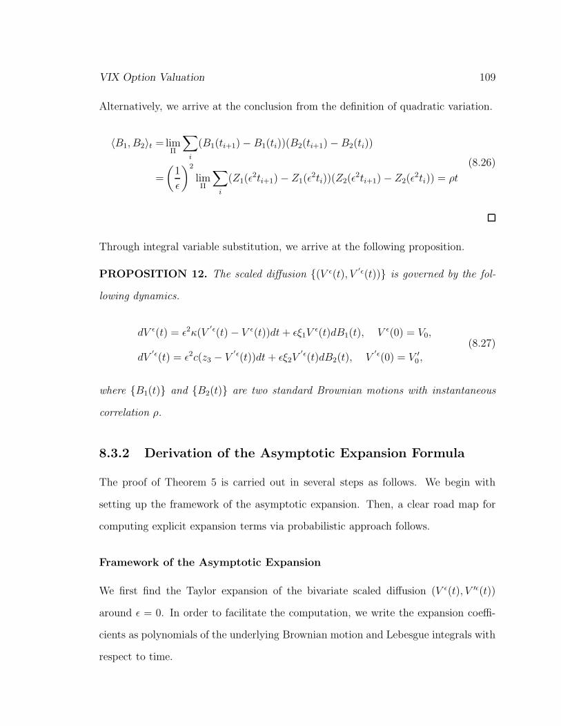
VIX Option Valuation 109
Alternatively, we arrive at the conclusion from the definition of quadratic variation.
〈B1, B2〉t = limΠ
∑
i
(B1(ti+1) − B1(ti))(B2(ti+1) − B2(ti))
=
(1
ǫ
)2
limΠ
∑
i
(Z1(ǫ2ti+1) − Z1(ǫ
2ti))(Z2(ǫ2ti+1) − Z2(ǫ
2ti)) = ρt
(8.26)
Through integral variable substitution, we arrive at the following proposition.
PROPOSITION 12. The scaled diffusion (V ǫ(t), V′ǫ(t)) is governed by the fol-
lowing dynamics.
dV ǫ(t) = ǫ2κ(V′ǫ(t) − V ǫ(t))dt + ǫξ1V
ǫ(t)dB1(t), V ǫ(0) = V0,
dV′ǫ(t) = ǫ2c(z3 − V
′ǫ(t))dt + ǫξ2V′ǫ(t)dB2(t), V
′ǫ(0) = V ′0 ,
(8.27)
where B1(t) and B2(t) are two standard Brownian motions with instantaneous
correlation ρ.
8.3.2 Derivation of the Asymptotic Expansion Formula
The proof of Theorem 5 is carried out in several steps as follows. We begin with
setting up the framework of the asymptotic expansion. Then, a clear road map for
computing explicit expansion terms via probabilistic approach follows.
Framework of the Asymptotic Expansion
We first find the Taylor expansion of the bivariate scaled diffusion (V ǫ(t), V ′ǫ(t))
around ǫ = 0. In order to facilitate the computation, we write the expansion coeffi-
cients as polynomials of the underlying Brownian motion and Lebesgue integrals with
respect to time.

VIX Option Valuation 110
PROPOSITION 13. The bivariate scaled diffusion (V ǫ(t), V ′ǫ(t)) admits the fol-
lowing Taylor expansion around ǫ = 0. For any n ∈ N, we have
V ǫ(t) =N∑
n=0
1
n!
∂nV ǫ(t)
∂ǫn
∣∣∣∣ǫ=0
ǫn + O(ǫN+1),
V ′ǫ(t) =
N∑
n=0
1
n!
∂nV ′ǫ(t)
∂ǫn
∣∣∣∣ǫ=0
ǫn + O(ǫN+1),
(8.28)
where the derivatives of (V ǫ(t), V ′ǫ(t)) w.r.t ǫ satisfy that
V ǫ(t)
∣∣∣∣ǫ=0
=V0,
∂V ǫ(t)
∂ǫ
∣∣∣∣ǫ=0
=ξ1V0B1(t),
∂2V ǫ(t)
∂ǫ2
∣∣∣∣ǫ=0
=2κ(V ′0 − V0)t + ξ2
1V0(B21(t) − t),
∂3V ǫ(t)
∂ǫ3
∣∣∣∣ǫ=0
=6κV ′0
∫ t
0
[ξ2B2(u) − ξ1B1(u)]du + t[6κξ1 (V ′0 − V0) − 3V0ξ
31 ]B1(t) + V0ξ
31B1(t)
3,
∂4V ǫ(t)
∂ǫ4
∣∣∣∣ǫ=0
=12κV ′0
∫ t
0
[ξ1B1(u) − ξ2B2(u)]2du + 24κξ1V′0B1(t)
∫ t
0
[ξ2B2(u) − ξ1B1(u)]du
+ t[12κξ21 (V ′
0 − V0) − 6V0ξ41 ]B1(t)
2 + V0ξ41B1(t)
4 + t2[12κ2 (V0 − V ′0)
+ 12κξ21 (V0 − V ′
0) + 3V0ξ41 + 12κc(z3 − V ′
0) + 6κV ′0(ξ
21 − ξ2
2)],
(8.29)
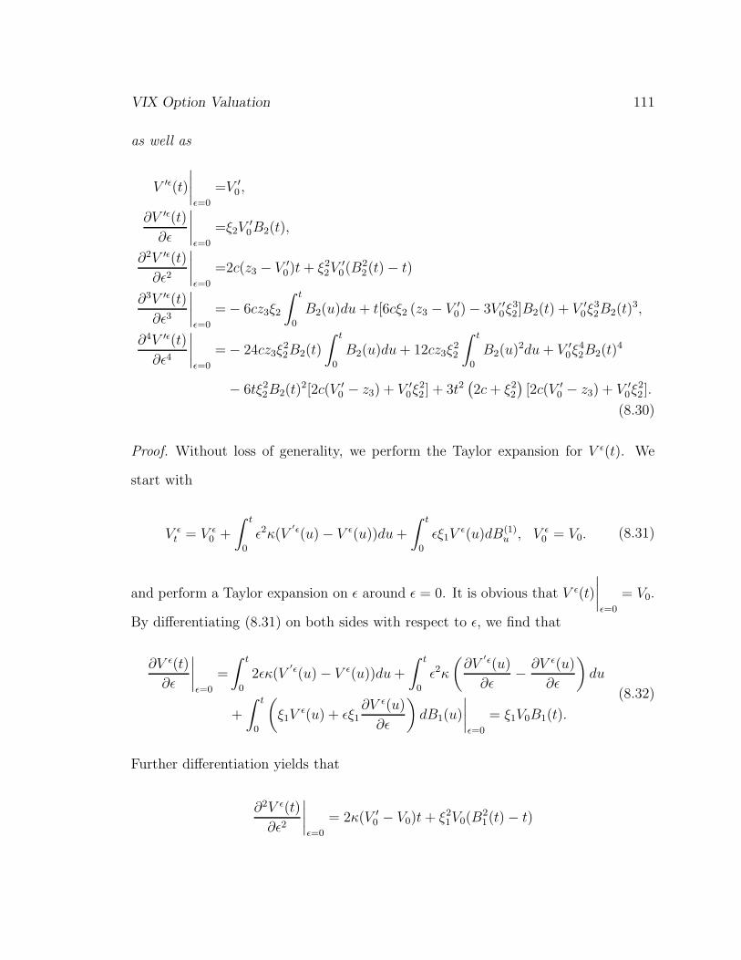
VIX Option Valuation 111
as well as
V ′ǫ(t)
∣∣∣∣ǫ=0
=V ′0 ,
∂V ′ǫ(t)
∂ǫ
∣∣∣∣ǫ=0
=ξ2V′0B2(t),
∂2V ′ǫ(t)
∂ǫ2
∣∣∣∣ǫ=0
=2c(z3 − V ′0)t + ξ2
2V′0(B
22(t) − t)
∂3V ′ǫ(t)
∂ǫ3
∣∣∣∣ǫ=0
= − 6cz3ξ2
∫ t
0
B2(u)du + t[6cξ2 (z3 − V ′0) − 3V ′
0ξ32]B2(t) + V ′
0ξ32B2(t)
3,
∂4V ′ǫ(t)
∂ǫ4
∣∣∣∣ǫ=0
= − 24cz3ξ22B2(t)
∫ t
0
B2(u)du + 12cz3ξ22
∫ t
0
B2(u)2du + V ′0ξ
42B2(t)
4
− 6tξ22B2(t)
2[2c(V ′0 − z3) + V ′
0ξ22 ] + 3t2
(2c + ξ2
2
)[2c(V ′
0 − z3) + V ′0ξ
22 ].
(8.30)
Proof. Without loss of generality, we perform the Taylor expansion for V ǫ(t). We
start with
V ǫt = V ǫ
0 +
∫ t
0
ǫ2κ(V′ǫ(u) − V ǫ(u))du +
∫ t
0
ǫξ1Vǫ(u)dB(1)
u , V ǫ0 = V0. (8.31)
and perform a Taylor expansion on ǫ around ǫ = 0. It is obvious that V ǫ(t)
∣∣∣∣ǫ=0
= V0.
By differentiating (8.31) on both sides with respect to ǫ, we find that
∂V ǫ(t)
∂ǫ
∣∣∣∣ǫ=0
=
∫ t
0
2ǫκ(V′ǫ(u) − V ǫ(u))du +
∫ t
0
ǫ2κ
(∂V
′ǫ(u)
∂ǫ− ∂V ǫ(u)
∂ǫ
)du
+
∫ t
0
(ξ1V
ǫ(u) + ǫξ1∂V ǫ(u)
∂ǫ
)dB1(u)
∣∣∣∣ǫ=0
= ξ1V0B1(t).
(8.32)
Further differentiation yields that
∂2V ǫ(t)
∂ǫ2
∣∣∣∣ǫ=0
= 2κ(V ′0 − V0)t + ξ2
1V0(B21(t) − t)
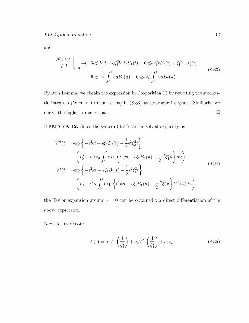
VIX Option Valuation 112
and
∂3V ǫ(t)
∂ǫ3
∣∣∣∣ǫ=0
=(−6κξ1V0t − 3ξ31V0t)B1(t) + 6κξ2V
′0tB2(t) + ξ3
1V0B31(t)
+ 6κξ1V′0
∫ t
0
udB1(u) − 6κξ2V′0
∫ t
0
udB2(u).
(8.33)
By Ito’s Lemma, we obtain the expression in Proposition 13 by rewriting the stochas-
tic integrals (Wiener-Ito chao terms) in (8.33) as Lebesgue integrals. Similarly, we
derive the higher order terms.
REMARK 12. Since the system (8.27) can be solved explicitly as
V ′ǫ(t) = exp
−ǫ2ct + ǫξ2B2(t) −
1
2ǫ2ξ2
2t
·(
V ′0 + ǫ2cz3
∫ t
0
exp
ǫ2cu − ǫξ2B2(u) +
1
2ǫ2ξ2
2u
du
);
V ǫ(t) = exp
−ǫ2κt + ǫξ1B1(t) −
1
2ǫ2ξ2
1t
·(
V0 + ǫ2κ
∫ t
0
exp
ǫ2κu − ǫξ1B1(u) +
1
2ǫ2ξ2
1u
V ′ǫ(u)du
),
(8.34)
the Taylor expansion around ǫ = 0 can be obtained via direct differentiation of the
above expression.
Next, let us denote
F (ǫ) = a1Vǫ
(1
ξ22
)+ a2V
′ǫ(
1
ξ22
)+ a3z3. (8.35)

VIX Option Valuation 113
By Taylor expansion, the underlying random variable in (8.23) reads
Xǫ =√
F (ǫ) =√
F (0) +F ′(0)
2√
F (0)ǫ +
1
2
[− F ′(0)2
4F (0)32
+F ′′(0)
2√
F (0)
]ǫ2
+1
6
[3F ′(0)3
8F (0)52
− 3F ′(0)F ′′(0)
4F (0)32
+F ′′′(0)
2√
F (0)
]ǫ3
+1
24
[F (4)(0)
2√
F (0)− 3F ′′(0)2
4F (0)3/2− 15F ′(0)4
16F (0)7/2− F (3)(0)F ′(0)
F (0)3/2+
9F ′(0)2F ′′(0)
4F (0)5/2
]ǫ4 + O(ǫ5),
(8.36)
where
F (0) = a1V0 + a2V′0 + a3z3,
and for n ∈ N,
F (n)(0) =
[a1
∂nV ǫ
∂ǫn
(1
ξ22
)+ a2
∂nV′ǫ
∂ǫn
(1
ξ22
)] ∣∣∣∣ǫ=0
. (8.37)
Employing a deterministic quantity ξ to be determined for computational purpose,
we rewrite that
Xǫ =√
F (ǫ) = X0 + ξ(ǫX1 + ǫ2X2 + ǫ3X3 + ǫ4X4 + O(ǫ5)),
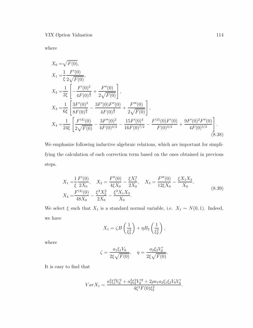
VIX Option Valuation 114
where
X0 =√
F (0),
X1 =1
ξ
F ′(0)
2√
F (0),
X2 =1
2ξ
[− F ′(0)2
4F (0)32
+F ′′(0)
2√
F (0)
],
X3 =1
6ξ
[3F ′(0)3
8F (0)52
− 3F ′(0)F ′′(0)
4F (0)32
+F ′′′(0)
2√
F (0)
],
X4 =1
24ξ
[F (4)(0)
2√
F (0)− 3F ′′(0)2
4F (0)3/2− 15F ′(0)4
16F (0)7/2− F (3)(0)F ′(0)
F (0)3/2+
9F ′(0)2F ′′(0)
4F (0)5/2
].
(8.38)
We emphasize following inductive algebraic relations, which are important for simpli-
fying the calculation of each correction term based on the ones obtained in previous
steps.
X1 =1
ξ
F ′(0)
2X0, X2 =
F ′′(0)
4ξX0− ξX2
1
2X0, X3 =
F ′′′(0)
12ξX0− ξX1X2
X0,
X4 =F (4)(0)
48X0− ξ2X2
2
2X0− ξ2X1X3
X0.
(8.39)
We select ξ such that X1 is a standard normal variable, i.e. X1 ∼ N(0, 1). Indeed,
we have
X1 = ζB
(1
ξ22
)+ ηB2
(1
ξ22
),
where
ζ =a1ξ1V0
2ξ√
F (0), η =
a2ξ2V′0
2ξ√
F (0).
It is easy to find that
V arX1 =a2
1ξ21V
20 + a2
2ξ22V
′20 + 2ρa1a2ξ1ξ2V0V
′0
4ξ2F (0)ξ22
.
VIX Option Valuation 115
Thus, ξ is selected according to
ξ =1
ξ2
√a2
1ξ21V
20 + a2
2ξ22V
′20 + 2ρa1a2ξ1ξ2V0V ′
0
4F (0).
We rewrite the strike as K = 100 × (X0 + ξǫy). Meanwhile, we define a translated
underlying variable
Y ǫ =Xǫ − X0
ǫξ= X1 + ǫX2 + ǫ2X3 + ǫ3X4 + O(ǫ4). (8.40)
REMARK 13. The reason why we define the translated variable Y ǫ is as follows.
We note that Y ǫ → X1 ∼ N(0, 1), as ǫ → 0 pathwise. The Malliavin non-degeneracy
of X1 allows us to obtain the uniform non-degeneracy of Y ǫ, which verifies the validity
of our asymptotic expansion. (See chapter 10 for detailed discussion.)
Let us denote f(x) = x+. Thus, we have that
CV IX0 = 100 × ξǫe
−r ǫ2
ξ22 EQf(Y ǫ − y).
In an appropriate weak sense,
∂
∂xf(x − y) = 1(y,+∞)(x),
∂2
∂x2f(x − y) = δy(x),
∂3
∂x3f(x − y) = δ′y(x),
where δy denotes the Dirac function centered at y. By Taylor expansion, we find that
f(Y ǫ − y) =N∑
n=0
1
n!
∂(n)
∂xnf(Y ǫ − y)
∣∣∣∣ǫ=0
ǫn + O(ǫN+1).
We denote Φn(y) = 1n!
∂(n)
∂xn f(Y ǫ − y)∣∣ǫ=0
and recall that

VIX Option Valuation 116
Y ǫ = X1 + ǫX2 + ǫ2X3 + ǫ3X4 + O(ǫ4),
where
X1 = Y 0, X2 =∂Y ǫ
∂ǫ
∣∣∣∣ǫ=0
, X3 =1
2
∂2Y ǫ
∂ǫ2
∣∣∣∣ǫ=0
, X4 =1
6
∂3Y ǫ
∂ǫ3
∣∣∣∣ǫ=0
.
Thus, we find that
Φ0(y) = (X1 − y)+,
Φ1(y) = 1(y,+∞)(X1)X2,
Φ2(y) =1
2
[δy(X1)X
22 + 1(y,+∞)(X1)(2X3)
],
Φ3(y) = δy(X1)X2X3 +1
6δ′y(X1)X
32 + 1(y,+∞)(X1)X4.
(8.41)
Next, we calculate the correction terms EQ[Φ0(y)], EQ[Φ1(y)], EQ[Φ2(y)] and EQ[Φ3(y)]
explicitly.
Preliminary Results on Brownian Moments
Our computation relies on the explicit knowledge of moments of the underlying Brow-
nian motion. In this section, we collect several auxiliary results which are useful for
the computation of each correction term.
PROPOSITION 14. For the two-dimensional Brownian motion B1(t), B2(t) and

VIX Option Valuation 117
any 0 < u ≤ t, we have the following conditional normal distributions.
B1(u)
B2(t)
∣∣∣∣ζB1(t) + ηB2(t) = y
∼N
utΩ1y
Ω2y
,
u − u2
tΩ1(ζ + ρη) ρu − uΩ1(η + ρζ)
ρu − uΩ1(η + ρζ) t − tΩ2(η + ρζ)
,
(8.42)
and
B1(t)
B2(u)
∣∣∣∣ζB1(t) + ηB2(t) = y
∼N
Ω1y
utΩ2y
,
t − tΩ1(ζ + ρη) ρu − uΩ1(η + ρζ)
ρu − uΩ1(η + ρζ) u − u2
tΩ1(η + ρζ)
,
(8.43)
and
B2(u)
B2(t)
∣∣∣∣ζB1(t) + ηB2(t) = y
∼N
utΩ2y
Ω2y
,
u − u2
tΩ2(η + ρζ) u − uΩ2(η + ρζ)
u − uΩ2(η + ρζ) t − tΩ2(η + ρζ)
,
(8.44)
and
B1(u)
B1(t)
∣∣∣∣ζB1(t) + ηB2(t) = y
∼N
utΩ1y
Ω1y
,
u − u2
tΩ1(ζ + ρη) u − uΩ1(ζ + ρη)
u − uΩ1(ζ + ρη) t − tΩ1(ζ + ρη)
,
(8.45)

VIX Option Valuation 118
where the various coefficients are defined in Theorem 5.
Without loss of generality, we verify the distributional property (8.42) for the case
u = t = 1ξ22, which is the key for deriving the first three correction terms. Let us
denote
Z1 =
B1
(1ξ22
)
B2
(1ξ22
)
, Z2 = ζB1
(1
ξ22
)+ ηB2
(1
ξ22
).
We note that (Z1, Z2)T is a three-dimensional normal variable N(µ, Σ), where
µ = (µ1, µ2)T = ((0, 0)T , 0)T
and
Σ =
Σ11 Σ12
Σ21 Σ22
=
1
ξ22
1 ρ
ρ 1
ζ + ρη
η + ρζ
(ζ + ρη η + ρζ
)ζ2 + η2 + 2ρζη
.
Thus, we have the following lemma, which appears as a special case of Proposition
14.
LEMMA 7.
(Z1|Z2 = y) ∼ N(µ(y), Σ),
where
µ =
µ1(y)
µ2(y)
= µ1 + Σ12Σ
−122 (y − µ2) =
y
ζ2 + η2 + 2ρζη
ζ + ρη
η + ρζ
(8.46)

VIX Option Valuation 119
and
Σ = (Σij)2×2 =
σ21 ρσ1σ2
ρσ1σ2 σ22
= Σ11−Σ12Σ
−122 Σ21 =
1
ξ22
1 − ρ2
ζ2 + η2 + 2ρζη
η2 −ζη
−ζη ζ2
,
(8.47)
with ρ = −1.
Based on Proposition 14 and Lemma 7, we are able to compute explicitly some Gaus-
sian moments, which are important to the calculation of the correction terms. For
example, we consider the case of u = t = 1/ξ22 . The conditional moment generating
function of (B1(t), B2(t)) given X1 = ζB1(t) + ηB2(t) = y is
M(ϑ1, ϑ2) := exp
µ1(y)ϑ1 + µ2(y)ϑ2 +
1
2ϑ2
1Σ11 + ϑ1ϑ2Σ12 +1
2ϑ2
2Σ22
, ϑ1, ϑ2 ∈ R.
Thus, the conditional moment satisfies
Mij := E[B1(t)iB2(t)
j |ζB1(t) + ηB2(t) = y] =∂i+j
∂iϑ1∂jϑ2
M(ϑ1, ϑ2)
∣∣∣∣ϑ1=ϑ2=0
.
Using this idea, we explicitly compute the following conditional Gaussian moments,
which are useful for the derivation of each correction term.
COROLLARY 5. For the two-dimensional Brownian motion B1(t), B2(t), the
following identities on conditional moments hold.

VIX Option Valuation 120
E (B1 (t) |ζB1(t) + ηB2(t) = x) =Ω1x,
E(B21 (t) |ζB1(t) + ηB2(t) = x) =Ω2
1x2 + σ2
1,
E(B31 (t) |ζB1(t) + ηB2(t) = x) =Ω3
1x3 + 3σ2
1Ω1x,
E(B41 (t) |ζB1(t) + ηB2(t) = x) =Ω4
1x4 + 6σ2
1Ω21x
2 + 3σ41,
E(B51 (t) |ζB1(t) + ηB2(t) = x) =Ω5
1x5 + 10σ2
1Ω31x
3 + 15Ω1σ41x,
E (B2 (t) |ζB1(t) + ηB2(t) = x) =Ω2x,
E(B22 (t) |ζB1(t) + ηB2(t) = x) =Ω2
2x2 + σ2
2,
E(B32 (t) |ζB1(t) + ηB2(t) = x) =Ω3
2x3 + 3σ2
2Ω2x,
E(B42 (t) |ζB1(t) + ηB2(t) = x) =Ω4
2x4 + 6σ2
2Ω22x
2 + 3σ42,
E(B52 (t) |ζB1(t) + ηB2(t) = x) =Ω5
2x5 + 10σ2
2Ω32x
3 + 15Ω2σ42x,
(8.48)
and
E(B1(u)|ζB1(t) + ηB2(t) = x) =u
t
x√ζ2 + η2 + 2ρζη
ρ13,
E(B21(u)|ζB1(t) + ηB2(t) = x) =ρ2
13[u(t − u)
t+ (
u
t)2 x2
ζ2 + η2 + 2ρζη] + (1 − ρ2
13)u,
E(B2(u)|ζB1(t) + ηB2(t) = x) =u
t
x√ζ2 + η2 + 2ρζη
ρ23,
E(B22(u)|ζB1(t) + ηB2(t) = x) =ρ2
23[u(t − u)
t+ (
u
t)2 x2
ζ2 + η2 + 2ρζη] + (1 − ρ2
23)u,
(8.49)
VIX Option Valuation 121
and
E(B1(t)2B2(t)|ζB1(t) + ηB2(t) = x) =Ω2
1Ω2x3 − 2σ1σ2Ω1x + σ2
1Ω2x,
E(B1(t)B2(t)2|ζB1(t) + ηB2(t) = x) =Ω1Ω
22x
3 − 2σ1σ2Ω2x + σ22Ω1x,
E(B1(t)3B2(t)
2|ζB1(t) + ηB2(t) = x) = − 6σ1σ2Ω21Ω2x
3 + (σ22 + x2Ω2
2)Ω31x
3 + 6σ21σ
22Ω1x
− 6σ31σ2Ω2x + 3σ2
1Ω1x(σ22 + x2Ω2
2),
E(B1(t)2B2(t)
3|ζB1(t) + ηB2(t) = x) = − 6σ1σ2Ω1Ω22x
3 + (σ21 + x2Ω2
1)Ω32x
3 + 6σ21σ
22Ω2x
− 6σ1σ32Ω1x + 3σ2
2Ω2x(σ21 + x2Ω2
1),
(8.50)
and
E(B1(u)B2(u)|ζB1(t) + ηB2(t) = x) =ρu − (η + ζρ)Ω1u2
t+
x2Ω1Ω2u2
t2,
E(B1(t)B2(u)|ζB1(t) + ηB2(t) = x) =uρ − u(η + ζρ)Ω1 +uΩ1Ω2x
2
t,
E(B1(t)B1(u)|ζB1(t) + ηB2(t) = x) =uρ2
13
t
x2
ζ2 + η2 + 2ρζη+ u(1 − ρ2
13),
E(B2(t)B2(u)|ζB1(t) + ηB2(t) = x) =uρ2
23
t
x2
ζ2 + η2 + 2ρζη+ u(1 − ρ2
23),
(8.51)

VIX Option Valuation 122
as well as
E(B1(t)2B1(u)|ζB1(t) + ηB2(t) = x) =2xΩ1 (u − u(ζ + ηρ)Ω1)
+uxΩ1 (x2Ω2
1 − t(ζ + ηρ)Ω1 + t)
t,
E(B1(t)2B2(u)|ζB1(t) + ηB2(t) = x) =2xΩ1 (uρ − u(ζ + ηρ)Ω2)
+uxΩ2 (x2Ω2
1 − t(ζ + ηρ)Ω1 + t)
t,
E(B1(u)B2(t)2|ζB1(t) + ηB2(t) = x) =2xΩ2 (uρ − u(η + ζρ)Ω1)
+uxΩ1 (x2Ω2
2 − t(η + ζρ)Ω2 + t)
t,
E(B2(u)B2(t)2|ζB1(t) + ηB2(t) = x) =2xΩ2 (u − u(η + ζρ)Ω2)
+uxΩ2 (x2Ω2
2 − t(η + ζρ)Ω2 + t)
t,
(8.52)
where the various coefficients are defined in Theorem 5.
Subsequently, we calculate each correction term explicitly. We exhibit the framework
and techniques employed in the computation as follows.
Calculation of the Leading Order Term: EQ[Φ0(y)]
It is easy to find that
EQ[Φ0(y)] =EQ(X1 − y)+ =
∫
R
(x − y)+φ(x)dx = yN(y) + φ(y) − y. (8.53)
Calculation of the Second Correction Term: EQ[Φ1(y)]
To begin with, we observe that
EQ[Φ1(y)] =EQ[1(y,+∞)(X1)X2] =
∫
R
EQ[1(y,+∞)(x)X2|X1 = x]φ(x)dx
=
∫ ∞
y
EQ[X2|X1 = x]φ(x)dx.
(8.54)

VIX Option Valuation 123
Thus, we focus on the calculation of conditional expectation EQ[X2|X1 = x] as follows.
We recall that
X1 = ζB1
(1
ξ22
)+ ηB2
(1
ξ22
).
By algebraic computation, we find that
X2 = −ξ2X21
2ξX0+
F ′′′(0)
4ξX0= α
(B1
(1
ξ22
))2
+ β
(B2
(1
ξ22
))2
+ γ + δX21 ,
where α, β, γ, δ, ζ, η are defined in Theorem 5. Hence, it follows from the computation
of moments based on Lemma 7 that
EQ[X2|X1 = x] = α(σ21 + µ2
1) + β(σ22 + µ2
2) + γ + δx2 = Λ0 + Λ1x2,
where
Λ0 = ασ21 + βσ2
2 + γ
and
Λ1 = αΩ21 + βΩ2
2 + δ.
Finally, we compute explicitly that
EQΦ1(y) =
∫ ∞
y
(Λ0 + Λ1x2)φ(x)dx = (Λ0 + Λ1)(1 − N(y)) + Λ1yφ(y).
Calculation of the Third Correction Term: EQ[Φ2(y)]
By conditioning, we have that

VIX Option Valuation 124
EQΦ2(y) =1
2
∫
R
E[δy(X1)X
22 + 1(y,+∞)(X1)(2X3)|X1 = x
]φ(x)dx
=1
2E(X2
2 |X1 = y)φ(y) +
∫ ∞
y
E(X3|X1 = x)φ(x)dx.
(8.55)
Denote the two-dimensional normal variable (B1, B2) ∼ N(µ, Σ). Thus, it is easy to
see that
E(X22 |X1 = y) = E(αB
2
1 + βB2
2 + γ + δy2)2.
By Lemma 7, we decompose the correlated normal variables as:
B1 =σ1W1 + µ1,
B2 =σ2(ρW1 +√
1 − ρ2W2) + µ2 = −σ2W1 + µ2,
(8.56)
where W1 ∼ N(0, 1). Using the fundamental fact
EWi = 0, EW 2i = 1, EW 3
i = 0, EW 4i = 3, for i=1, 2,
we find that
Λ2 := E(X22 |X1 = y) = 3ω2
2(y) + ω21(y) + ω2
0(y) + 2ω0(y)ω2(y), (8.57)
where
ω0(y) = (αΩ21 + βΩ2
2 + δ)y2 + γ, ω1(y) = (2ασ1Ω1 − 2βσ2Ω2)y, ω2(y) = ασ21 + βσ2
2.
(8.58)
Now, we compute the conditional expectation E(X3|X1 = x). It is straightforward to
find that
E(X3|X1 = x) = θ7x + θ8x3 +
1
12ξX0E(F ′′′(0)|X1 = x)

VIX Option Valuation 125
where
F ′′′(0) = θ1B1
(1
ξ22
)+θ2B2
(1
ξ22
)+θ3B
31
(1
ξ22
)+θ4B
32
(1
ξ22
)+θ5
∫ 1
ξ22
0
udB1(u)+θ6
∫ 1
ξ22
0
udB2(u),
with the coefficients defined in the Theorem 5. By Corollary 5, we have that
E
(B1
(1
ξ22
) ∣∣∣∣X1 = x
)= Ω1x,
E
(B2
(1
ξ22
) ∣∣∣∣X1 = x
)= Ω2x,
E
(B3
1
(1
ξ22
) ∣∣∣∣X1 = x
)= µ3
1 + 3µ1σ21 = Ω3
1x3 + 3σ2
1Ω1x,
E
(B3
2
(1
ξ22
) ∣∣∣∣X1 = x
)= µ3
2 + 3µ2σ22 = Ω3
2x3 + 3σ2
2Ω2x,
E
(∫ 1
ξ22
0
udB1(u)
∣∣∣∣X1 = x
)=
ρ13
2ξ22
x√ζ2 + η2 + 2ρζη
=Ω1
2ξ22
x,
E
(∫ 1
ξ22
0
udB2(u)
∣∣∣∣X1 = x
)=
ρ23
2ξ22
x√ζ2 + η2 + 2ρζη
=Ω2
2ξ22
x,
(8.59)
where
Ω1 =ζ + ρη
ζ2 + η2 + 2ρζη, Ω2 =
η + ρζ
ζ2 + η2 + 2ρζη,
and
ρ13 =ζ + ρη√
ζ2 + η2 + 2ρζη, ρ23 =
η + ρζ√ζ2 + η2 + 2ρζη
.
REMARK 14. (A Brownian-Bridge-Based Calculation) The above identities can
be alternatively obtained from the Cholesky decomposition of correlated Brownian
motions and the properties of Brownian bridge. We let
B3(w) =ζB1(w) + ηB2(w)√
ζ2 + η2 + 2ρζη,

VIX Option Valuation 126
which forms a standard Brownian motion B3(t) satisfying
Corr(dB1, dB3) = ρ13dt, Corr(dB2, dB3) = ρ23dt.
Thus,
E
(∫ 1
ξ22
0
udBi(u)
∣∣∣∣X1 = x
)= E
(∫ w
0
udBi(u)
∣∣∣∣B3(w) =x√
ζ2 + η2 + 2ρζη
), (8.60)
where w = 1ξ22. To compute this expectation, we first observe that
∫ w
0
udBi(u) = wBi(w) −∫ w
0
Bi(u)du. (8.61)
It is easy to obtain that, for i = 1, 2,
Bi(t) = ρi3B3(t) +√
1 − ρ2i3B
′i(t), (8.62)
where B′i(t) is a Brownian motion independent of B3(t). So, equation (8.60) can
be further deduced from interchanging the order of conditional expectation and the
Lebesgue integration on time, i.e.
E
(∫ 1
ξ22
0
udBi(u)
∣∣∣∣X1 = x
)
=E
(wBi(w)
∣∣∣∣B3(w) =x√
ζ2 + η2 + 2ρζη
)− E
(∫ w
0
Bi(u)du
∣∣∣∣B3(w) =x√
ζ2 + η2 + 2ρζη
)
=wE
(Bi(w)
∣∣∣∣B3(w) =x√
ζ2 + η2 + 2ρζη
)−∫ w
0
E
(Bi(u)
∣∣∣∣B3(w) =x√
ζ2 + η2 + 2ρζη
)du.
(8.63)
VIX Option Valuation 127
Based on the property of Brownian bridge, we observe that
E
(B3(u)
∣∣∣∣B3(w) =x√
ζ2 + η2 + 2ρζη
)=
u
w
x√ζ2 + η2 + 2ρζη
. (8.64)
This, we complete the computation of (8.60).
Finally, it follows that
E(X3|X1 = x) = Λ3x + Λ4x3,
where
Λ3 = θ7 +1
12ξX0
(θ1Ω1 + θ2Ω2 + 3θ3Ω1σ
21 + 3θ4Ω2σ
22 +
θ5Ω1
2ξ22
+θ6Ω2
2ξ22
),
Λ4 = θ8 +1
12ξX0
(θ3Ω
31 + θ4Ω
32
).
(8.65)
Hence, by explicit integration we find that
∫ +∞
y
E(X3|X1 = x)φ(x)dx =
∫ +∞
y
(Λ3x + Λ4x3)φ(x)dx = φ(y)(Λ3 + (2 + y2)Λ4).
Calculation of the Fourth Correction Term: EQ[Φ3(y)]
We briefly outline the framework and techniques for computing the fourth order
correction term in this section. First, by conditioning, we have that
EΦ3(y) =
∫ +∞
−∞E(Φ3(y)|X1 = x)φ(x)dx, (8.66)
where
E(Φ3(y)|X1 = x) =E(δy(X1)X2X3|X1 = x)
+1
6E(δ′y(X1)X
32 |X1 = x) + E(1(y,+∞)(X1)X4|X1 = x).
(8.67)

VIX Option Valuation 128
Therefore, we find that
EΦ3(y) = A(y) + B(y) + C(y),
where
A(y) = E(X2X3|X1 = y)φ(y),
B(y) = −1
6
∂
∂yE(X3
2 |X1 = y)φ(y),
C(y) =
∫ +∞
y
E(X4|X1 = x)φ(x)dx.
(8.68)
Here, we have used the following integration by parts formula for Dirac Delta function,
i.e. for any function g and n ∈ N,
∫ +∞
−∞g(x)δ(n)
y (x)dx = −∫ +∞
−∞
∂g
∂x(x)δ(n−1)
y (x)dx.
Next, we compute A(y), B(y) and C(y), respectively.
We begin with the following inductive algebraic relations, which allow us to make
use of the previous computation results to derive new ones. These observations are
helpful for reducing the computational load.
X2 =F ′′(0)
4ξX0− ξX2
1
2X0, X3 =
F ′′′(0)
12ξX0− ξX1X2
X0, X4 =
F (4)(0)
48X0− ξ2X2
2
2X0− ξ2X1X3
X0.
(8.69)
For term A(y), we have that
A(y) =
1
12ξX0
[1
4ξX0E(F ′′(0)F ′′′(0)|X1 = y) − ξy2
2X0E(F ′′′(0)|X1 = y)
]
− ξy
X0E(X2
2 |X1 = y)
φ(y),
(8.70)
where
VIX Option Valuation 129
E(X22 |X1 = y) = 3ω2
2(y) + ω21(y) + ω2
0(y) + 2ω0(y)ω2(y),
and
E(F ′′′(0)|X1 = y) = 12ξX0[(Λ3 − θ7)y + (Λ4 − θ8)y3],
and E(F ′′(0)F ′′′(0)|X1 = y) is a new quantity to compute. Based on (8.37), F ′′(0)F ′′′(0)
can be expanded explicitly as a combination of polynomials and Lebesgue integrals,
with respect to time, of the underlying Brownian motions. Thus, we accomplish the
explicit computation of conditional moments by using the identities in Corollary 5.
Without loss of generality, we demonstrate the computation on one of such terms.
For example, we need to compute
E
[B1(t)
2
∫ t
0
B2(u)du
∣∣∣∣ζB1(t) + ηB2(t) = x
].
Indeed, this conditional expectation is equal to
∫ t
0
E(B1(t)2B2(u)|ζB1(t) + ηB2(t) = x)du
=
∫ t
0
[2xΩ1 (uρ − u(ζ + ηρ)Ω2) +
uxΩ2 (x2Ω21 − t(ζ + ηρ)Ω1 + t)
t
]du
=1
2tΩ2
1Ω2y3 +
(t2ρΩ1 +
1
2t2Ω2 −
3
2t2ζΩ1Ω2 −
3
2t2ηρΩ1Ω2
)y.
(8.71)
VIX Option Valuation 130
For term B(y), we observe that
EQ(X32 |X1 = y)
=E(αB2
1 + βB2
2 + γ + δy2)3
=E(α(σ1W1 + µ1)2 + β(−σ2W1 + µ2)
2 + γ + δy2)3
=E(ω2(y)W 21 + ω1(y)W1 + ω0(y))3
=15ω2(y)3 + 9ω0(y)ω2(y)2 + 3(ω0(y)2ω2(y) + ω0(y)ω1(y)2) + ω0(y)3.
(8.72)
For term C(y), we observe that
E(X4|X1 = x) =1
48X0E(F (4)(0)|X1 = x) − ξ2
2X0E(X2
2 |X1 = x) − ξ2x
X0E(X3|X1 = x),
where it is known from the previous computation that
E(X22 |X1 = x) = 3ω2
2(x) + ω21(x) + ω2
0(x) + 2ω0(x)ω2(x),
and that
E(X3|X1 = x) = Λ3x + Λ4x3.
For any constants ci, i = 1, ..., 5, we have that
∫ +∞
y
(c0 + c1x + c2x2 + c3x
3 + c4x4)φ(x)dx
=(c0 + c2 + 3c4)(1 − N(y)) + φ(y)[(c1 + 2c3) + (c2 + 3c4)y + c3y2 + c4y
3].
(8.73)
This fact renders an explicit calculation of term C(y).
Finally, the price of VIX option CV IX0 (see (8.23)) admits the following asymptotic

VIX Option Valuation 131
expansion:
CV IX0 = 100 × ξe
−r ǫ2
ξ22
ǫΘ1(y) + ǫ2Θ2(y) + ǫ3Θ3(y) + ǫ4Θ4(y) + O(ǫ5)
, (8.74)
where
Θ1(y) =φ(y) − y(1 − N(y)),
Θ2(y) =(Λ0 + Λ1)(1 − N(y)) + Λ1yφ(y),
Θ3(y) =1
2Λ2φ(y) + φ(y)(Λ3 + (2 + y2)Λ4),
Θ4(y) =(Λ5y
7 + Λ6y5 + Λ7y
3 + Λ8y)φ(y) + 2Λ9(1 − N(y)).
(8.75)

Chapter 9
Implementation and Numerical
Examples
In this chapter, we demonstrate the efficiency of our asymptotic expansion formula
in Theorem 5 with some numerical experiments. First, we employ a bias-corrected
Monte Carlo simulation scheme as a benchmark, to which the implementation of the
formula is compared. We recall that
CV IX0 = 100 × e−rT E
(√a1VT + a2V ′
T + a3z3 −K
100
)+
.
9.1 Benchmark from Monte Carlo Simulation: Eu-
ler Scheme with Partial Truncation
Due to the positivity of the diffusion processes (Vt, V′t ), we adopt a biased-corrected
Euler discretization scheme of partial truncation (see Lord et al. (2008)[76]). By the
132

Implementation and Numerical Examples 133
Cholesky decomposition of Brownian motion, we rewrite the dynamics of (Vt, V′t ) as
follows
dVt =κ(V ′t − Vt)dt + ξ1Vtdβ1(t),
dV ′t =c(z3 − V ′
t )dt + ξ2V′t d[ρdβ1(t) +
√1 − ρ2dβ2(t)],
(9.1)
where (β1(t), β2(t)) is a standard two-dimensional Brownian motion. Thus the
partial truncation scheme can be designed as
Vi+1 =Vi + κ(V ′i − Vi)∆t + ξ1(Vi ∨ 0)
√∆tZ
(1)i ,
V ′i+1 =V ′
i + c(z3 − V ′i )∆t + ξ2(V
′i ∨ 0)[ρ
√∆tZ
(1)i +
√1 − ρ2
√∆tZ
(2)i ],
(9.2)
where Z(1)i , Z
(2)i is an independent two-dimensional standard normal sequences. In
the implementation, we choose a reasonable length of the time step and number of
simulation trials to minimize the mean square error.
9.2 Implementation of our Asymptotic Expansion
Formula
To demonstrate the numerical performance of our asymptotic expansion formula, we
use model parameters similar to those estimated in Gatheral (2008) [50, 51], which
were found by calibrating the model to the market VIX option prices data in April
2007. We adjust the value of parameter ξ2 slightly so that the stability condition (7.13)
is satisfied. We assume a risk free rate of 4.00%. Table 9.1 gives this parameter set.
Accordingly, the initial value for VIX is calculated as VIX0 = 17.47. We conduct
numerical experiments to compute the prices of options on VIX for different strikes
and maturities. Because of the large trading volume and the high liquidity of options

Implementation and Numerical Examples 134
on VIX with strikes around the initial value of the underlying VIX, we select the
range of strikes used for our numerical illustration to be from 14 to 23. For each case,
we compare the computing performance of the formulae employing the expansion
up to indicated order of convergence, including O(ǫ5),O(ǫ4),O(ǫ3) and O(ǫ2). We
regard the Monte Carlo simulation results as benchmark. In Table 9.2, all numerical
results are exhibited. It takes about 60 milliseconds to compute one value from our
asymptotic expansion formula while the simulation takes much longer time, on average
about 230 CPU seconds for each by sampling 103 time steps with 106 simulation trials,
in order to achieve satisfactory level of standard error (in the magnitude of 10−5 in
our examples shown in Table 9.2). We can observe a significant saving in computing
time using our asymptotic expansion formula as compared to Monte Carlo simulation.
INPUT PARAMETERS ValuesRisk Free Rate r 0.04Time Horizon of VIX ∆T 0.082Correlation ρ 0.57Initial Instantaneous Variance V0 0.0137Initial Intermediate Level V ′
0 0.0208Long-Term Intermediate Level z3 0.078Rate of Mean Reversion κ 5.5Rate of Mean Reversion c 0.1Volatility of the Instantaneous Variance ξ1 2.6Volatility of the Intermediate Level ξ2 0.44
Table 9.1: Input Parameters
Also, we plot the “value matching” between asymptotic expansion valuation and
Monte Carlo simulation. We observe that the satisfactory fitting of the VIX option
prices is obtained for actively traded short maturity (for example, up to one-month)
options as shown in Figure 9.1. Motivated by the geometric Brownian motion model
for VIX in Whaley (1993) [91], in the numerical comparison between our asymptotic
expansion formula and Monte Carlo simulation, we also convert the VIX option prices

Implementation and Numerical Examples 135
computed from both of the two approaches into the Black-Scholes implied volatility.
From Figure 9.2, we observe the fitting of the Black-Scholes implied volatility for the
relatively short maturities, one-month at least, and the deviation magnified at the
out-of-money side. We also plot and illustrate the computing errors from applying
the formulae with various convergence orders, including O(ǫ5),O(ǫ4),O(ǫ3) and O(ǫ2)
in Figure 9.3(a). For the sake of completeness, we plot the absolute errors in Fig-
ure 9.3(b). We observe the significant improvement on the numerical performance
by adding more correction terms in our asymptotic expansion. All implementations
algorithms are programmed in C++ and executed on a laptop PC with a Intel(R)
Pentium(R) M 1.73GHz processor and 1GB of RAM running Windows XP Profes-
sional.
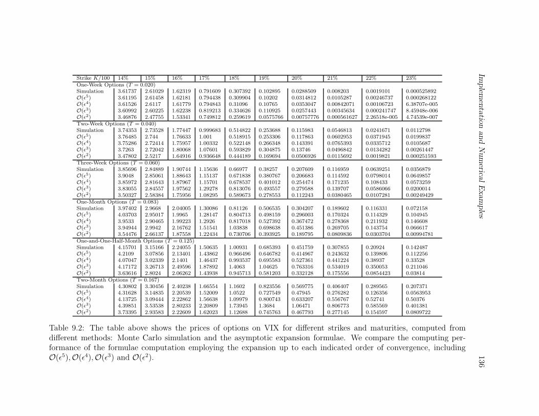
Implem
enta
tion
and
Num
ericalE
xam
ples
136
Strike K/100 14% 15% 16% 17% 18% 19% 20% 21% 22% 23%One-Week Options (T = 0.020)Simulation 3.61737 2.61029 1.62319 0.791609 0.307392 0.102895 0.0288509 0.008203 0.0019101 0.000525892O(ǫ5) 3.61195 2.61458 1.62181 0.794438 0.309904 0.10202 0.0314812 0.0105287 0.00246737 0.000268122O(ǫ4) 3.61526 2.6117 1.61779 0.794843 0.31096 0.10765 0.0353047 0.00842071 0.00106723 6.38707e-005O(ǫ3) 3.60992 2.60225 1.62238 0.819213 0.334626 0.110925 0.0257443 0.00345634 0.000241747 8.45948e-006O(ǫ2) 3.46876 2.47755 1.53341 0.749812 0.259619 0.0575766 0.00757776 0.000561627 2.26518e-005 4.74539e-007Two-Week Options (T = 0.040)Simulation 3.74353 2.73528 1.77447 0.999683 0.514822 0.253688 0.115983 0.0546813 0.0241671 0.0112798O(ǫ5) 3.76485 2.744 1.76633 1.001 0.518915 0.253306 0.117863 0.0602953 0.0371945 0.0199837O(ǫ4) 3.75286 2.72414 1.75957 1.00332 0.522148 0.266348 0.143391 0.0765393 0.0335712 0.0105687O(ǫ3) 3.7263 2.72042 1.80068 1.07601 0.593829 0.304875 0.13746 0.0496842 0.0134282 0.00261447O(ǫ2) 3.47802 2.5217 1.64916 0.936648 0.444189 0.169694 0.0506926 0.0115692 0.0019821 0.000251593Three-Week Options (T = 0.060)Simulation 3.85696 2.84889 1.90744 1.15636 0.66977 0.38257 0.207609 0.116959 0.0639251 0.0356879O(ǫ5) 3.9048 2.85061 1.88643 1.15137 0.671838 0.380767 0.206683 0.114592 0.0798014 0.0649857O(ǫ4) 3.85972 2.81643 1.87967 1.15701 0.678537 0.401012 0.254474 0.171235 0.108433 0.0573259O(ǫ3) 3.83055 2.84557 1.97562 1.29278 0.813076 0.493557 0.279588 0.139707 0.0586066 0.0200014O(ǫ2) 3.50327 2.58384 1.75956 1.08295 0.589673 0.278553 0.112243 0.0380465 0.0107281 0.00249429One-Month Options (T = 0.083)Simulation 3.97402 2.9668 2.04005 1.30086 0.81126 0.506535 0.304207 0.189602 0.116331 0.072158O(ǫ5) 4.03703 2.95017 1.9965 1.28147 0.804713 0.498159 0.296003 0.170324 0.114329 0.104945O(ǫ4) 3.9533 2.90465 1.99223 1.2926 0.817018 0.527392 0.367472 0.278368 0.211932 0.146608O(ǫ3) 3.94944 2.9942 2.16762 1.51541 1.03838 0.698638 0.451386 0.269705 0.143754 0.066617O(ǫ2) 3.54476 2.66137 1.87558 1.22434 0.730706 0.393925 0.189795 0.0809836 0.0303704 0.00994781One-and-One-Half-Month Options (T = 0.125)Simulation 4.15701 3.15166 2.24055 1.50635 1.00931 0.685393 0.451759 0.307855 0.20924 0.142487O(ǫ5) 4.2109 3.07856 2.13401 1.43862 0.966496 0.646782 0.414967 0.243632 0.139806 0.112256O(ǫ4) 4.07047 3.02339 2.1401 1.46437 0.993537 0.695583 0.527361 0.441224 0.38937 0.33528O(ǫ3) 4.17172 3.26713 2.49596 1.87892 1.4063 1.04625 0.763316 0.534019 0.350053 0.211046O(ǫ2) 3.63616 2.8024 2.06262 1.43938 0.945713 0.581203 0.332128 0.175556 0.0854423 0.03814Two-Month Options (T = 0.167)Simulation 4.30802 3.30456 2.40238 1.66554 1.1602 0.823556 0.569775 0.406407 0.289565 0.207371O(ǫ5) 4.31628 3.14835 2.20539 1.52009 1.0522 0.727549 0.47945 0.276282 0.126356 0.0563953O(ǫ4) 4.13725 3.09444 2.22862 1.56638 1.09979 0.800743 0.633207 0.556767 0.52741 0.50376O(ǫ3) 4.39851 3.53538 2.80233 2.20809 1.73945 1.3684 1.06471 0.806773 0.585569 0.401381O(ǫ2) 3.73395 2.93583 2.22609 1.62023 1.12688 0.745763 0.467793 0.277145 0.154597 0.0809722
Table 9.2: The table above shows the prices of options on VIX for different strikes and maturities, computed fromdifferent methods: Monte Carlo simulation and the asymptotic expansion formulae. We compare the computing per-formance of the formulae computation employing the expansion up to each indicated order of convergence, includingO(ǫ5),O(ǫ4),O(ǫ3) and O(ǫ2).

Implementation and Numerical Examples 137
0.15 0.16 0.17 0.18 0.19 0.2 0.21 0.22 0.230
0.5
1
1.5
2
2.5
3
3.5
4
Strike/100
VIX
Opt
ion
Pric
eComparison of the Valuation for One−week VIX Options from Two Approaches for Each Strike
Monte Carlo SimulationAsymptotic Expansion
(a) One-week
0.15 0.16 0.17 0.18 0.19 0.2 0.21 0.22 0.230
0.5
1
1.5
2
2.5
3
3.5
4
Strike/100
VIX
Opt
ion
Pric
e
Comparison of the Valuation for Two−week VIX Options from Two Approaches for Each Strike
Monte Carlo SimulationAsymptotic Expansion
(b) Two-week
0.15 0.16 0.17 0.18 0.19 0.2 0.21 0.22 0.230
0.5
1
1.5
2
2.5
3
3.5
4
Strike/100
VIX
Opt
ion
Pric
e
Comparison of the Valuation for Three−week VIX Options from Two Approaches for Each Strike
Monte Carlo SimulationAsymptotic Expansion
(c) Three-week
0.15 0.16 0.17 0.18 0.19 0.2 0.21 0.22 0.230
0.5
1
1.5
2
2.5
3
3.5
4
Strike/100
VIX
Opt
ion
Pric
e
Comparison of the Valuation for One−month VIX Options from Two Approaches for Each Strike
Monte Carlo SimulationAsymptotic Expansion
(d) One-month
0.15 0.16 0.17 0.18 0.19 0.2 0.21 0.22 0.230
0.5
1
1.5
2
2.5
3
3.5
4
4.5
Strike/100
VIX
Opt
ion
Pric
e
Comparison of the Valuation for One−and−a−half−month VIX Options from Two Approaches for Each Strike
Monte Carlo SimulationAsymptotic Expansion
(e) One-and-a-half-month
0.15 0.16 0.17 0.18 0.19 0.2 0.21 0.22 0.230
0.5
1
1.5
2
2.5
3
3.5
4
4.5
Strike/100
VIX
Opt
ion
Pric
e
Comparison of the Valuation for Two−month VIX Options from Two Approaches for Each Strike
Monte Carlo SimulationAsymptotic Expansion
(f) Two-month
Figure 9.1: This set of graphs illustrates the comparison of the VIX option pricescomputed from the Monte Carlo simulation and our O(ǫ5) asymptotic expansion.The maturities range from one week to two month.

Implementation and Numerical Examples 138
0.15 0.16 0.17 0.18 0.19 0.2 0.21 0.22 0.230.5
0.6
0.7
0.8
0.9
1
1.1
1.2
1.3
Strike/100
Impl
ied
Vol
atili
tyComparison of the Black−Scholes Implied Volatility for One−week VIX Options
Monte Carlo SimulationAsymptotic Expansion
(a) One-week
0.15 0.16 0.17 0.18 0.19 0.2 0.21 0.22 0.230.5
0.6
0.7
0.8
0.9
1
1.1
1.2
Strike/100
Impl
ied
Vol
atili
ty
Comparison of the Black−Scholes Implied Volatility for Two−week VIX Options
Monte Carlo SimulationAsymptotic Expansion
(b) Two-week
0.15 0.16 0.17 0.18 0.19 0.2 0.21 0.22 0.230.5
0.6
0.7
0.8
0.9
1
1.1
1.2
Strike/100
Impl
ied
Vol
atili
ty
Comparison of the Black−Scholes Implied Volatility for Three−week VIX Options
Monte Carlo SimulationAsymptotic Expansion
(c) Three-week
0.15 0.16 0.17 0.18 0.19 0.2 0.21 0.22 0.230.5
0.55
0.6
0.65
0.7
0.75
0.8
0.85
0.9
0.95
Strike/100
Impl
ied
Vol
atili
ty
Comparison of the Black−Scholes Implied Volatility for One−month VIX Options
Monte Carlo SimulationAsymptotic Expansion
(d) One-month
0.15 0.16 0.17 0.18 0.19 0.2 0.21 0.22 0.230.45
0.5
0.55
0.6
0.65
0.7
0.75
0.8
0.85
0.9
Strike/100
Impl
ied
Vol
atili
ty
Comparison of the Black−Scholes Implied Volatility for One−and−a−half−month VIX Options
Monte Carlo SimulationAsymptotic Expansion
(e) One-and-a-half-month
0.15 0.16 0.17 0.18 0.19 0.2 0.21 0.22 0.230.35
0.4
0.45
0.5
0.55
0.6
0.65
0.7
0.75
0.8
0.85
Strike/100
Impl
ied
Vol
atili
ty
Comparison of the Black−Scholes Implied Volatility for Two−month VIX Options
Monte Carlo SimulationAsymptotic Expansion
(f) Two-month
Figure 9.2: This set of graphs illustrates the comparison of the Black-Scholes impliedvolatilities computed from the Monte Carlo simulation and our O(ǫ5) asymptoticexpansion. The maturities range from one week to two month.
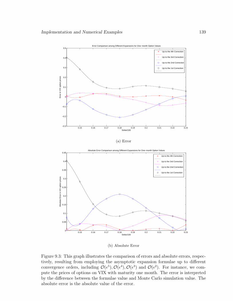
Implementation and Numerical Examples 139
0.15 0.16 0.17 0.18 0.19 0.2 0.21 0.22 0.23−0.3
−0.2
−0.1
0
0.1
0.2
0.3
0.4
0.5
Strike/100
Err
or in
VIX
opt
ion
pric
es
Error Comparison among Different Expansions for One−month Option Values
Up to the 4th Correction
Up to the 3rd Correction
Up to the 2nd Correction
Up to the 1st Correction
(a) Error
0.15 0.16 0.17 0.18 0.19 0.2 0.21 0.22 0.230
0.05
0.1
0.15
0.2
0.25
0.3
0.35
0.4
0.45
Strike/100
Abs
olut
e E
rror
in V
IX o
ptio
n pr
ices
Absolute Error Comparison among Different Expansions for One−month Option Values
Up to the 4th Correction
Up to the 3rd Correction
Up to the 2nd Correction
Up to the 1st Correction
(b) Absolute Error
Figure 9.3: This graph illustrates the comparison of errors and absolute errors, respec-tively, resulting from employing the asymptotic expansion formulae up to differentconvergence orders, including O(ǫ5),O(ǫ4),O(ǫ3) and O(ǫ2). For instance, we com-pute the prices of options on VIX with maturity one month. The error is interpretedby the difference between the formulae value and Monte Carlo simulation value. Theabsolute error is the absolute value of the error.

Chapter 10
On the Validity of the Asymptotic
Expansion
In this chapter, we justify the validity of our asymptotic expansion in Theorem 5.
The following theorem characterizes the magnitude of the asymptotic error explicitly.
THEOREM 6. Let us denote CV IX0 (k) the price of VIX option with strike k. There
exists R > 0, such that, for any N ∈ N, we have
∣∣∣∣CV IX0 (100 × (X0 + ǫξy)) − 100 × ξe
−r ǫ2
ξ22
N∑
k=1
ǫkΘk(y)
∣∣∣∣ ≤ RǫN+1,
where the various quantities are defined in Theorem 5.
We employ the Malliavin-Watanabe-Yoshida theory on asymptotic expansion for gen-
eralized Wiener functional to justify Theorem 6. For the reader’s convenience, we
document a brief introduction to the theory of Malliavin calculus and the Malliavin-
Watanabe-Yoshida theory on asymptotic expansion, where the Watanabe theory
(1987) [90] and its further refinement by Yoshida [93, 92, 94] are briefly surveyed.
140

On the Validity of the Asymptotic Expansion 141
First of all, we establish the following proposition which leads to Theorem 6.
PROPOSITION 15. For any arbitrary y ∈ R and f(x) = max(x, 0), we have that
|EQf(Y ǫ − y) − EQ[Φ0(y) + ǫΦ1(y) + ǫ2Φ2(y) + ǫ3Φ3(y)]| ≤ Rǫ4, (10.1)
for some constant R > 0, where Φi(y), i = 1, 2, 3, 4, are defined in (8.41).
The proof of Proposition 15 is carried out in several steps as follows. We sketch the
proof and omit some tedious routine details. In the proof, the notations related to
the Malliavin calculus are explained in Appendix 10.
First of all, by the Cholesky decomposition, we identify a two-dimensional Wiener
process W1(t), W2(t) such that
B1(t) = W1(t),
B2(t) = ρW1(t) +√
1 − ρ2W2(t).
(10.2)
In the following exposition, our justification is carried out on the two-dimensional
Wiener space associated to W1(t), W2(t).
Because the SDE system is linear, by Theorem 2.2.2 of Nualart (2006), the bivari-
ate random variable (V ǫ(t), V ′ǫ(t)) is in D∞. Based on Theorem 7.1 in Malliavin
and Thalmaier (2004) [78] and Theorem 3.3 in Watanabe (1987), we find that the
coefficients for the asymptotic expansion of (V ǫ(t), V ′ǫ(t)) in Proposition 13 are in
D∞; the asymptotic expansion (8.28) lies in D∞. Let us regard Xǫ as a function
G(v, v′) =√
a1v + a2v′ + a3z3 acting on the positive diffusion (V ǫ(t), V ′ǫ(t)). Em-
ploying the chain rule and Proposition 1.5.1 in Nualart (2006) [80], we obtain that
Xǫ ∈ D∞. Noticing the expression of the coefficients in the expansion of Xǫ, we claim

On the Validity of the Asymptotic Expansion 142
that Xi ∈ D∞, for i = 0, 1, 2, .... Following an argument using elementary Taylor ex-
pansion as in Chapter. 7 of Malliavin and Thalmaier (2004) [78], we obtain that, for
any n ∈ N,
∥∥∥∥Xǫ −n∑
k=0
1
k!
∂kXǫ
∂ǫk
∣∣∣∣ǫ=0
ǫk
∥∥∥∥Ds
p
= O(ǫn+1), for any s > 0, p ∈ N. (10.3)
i.e.
∥∥∥∥∥Xǫ −(
X0 + ξn∑
k=1
ǫkXk
)∥∥∥∥∥Ds
p
= O(ǫn+1), for any s > 0, p ∈ N. (10.4)
Without loss of generality, we sketch the proof of (10.4) for the case of n = 1:
‖Xǫ − (X0 + ǫξX1)‖Dsp
= O(ǫ2). (10.5)
Indeed, by the integral form of Taylor expansion and integration variable substitution,
we deduce that
Xǫ − (X0 + ǫξX1) =Xǫ − X0 −∂X
∂ǫ
∣∣∣∣ǫ=0
ǫ
=
∫ ǫ
0
∫ u
0
∂2X
∂ǫ2
∣∣∣∣ǫ=s
dsdu
=ǫ2
∫ 1
0
∫ w
0
2F ′′(rǫ)F (rǫ) − F ′(rǫ)2
4F (rǫ)32
drdw.
(10.6)
Because
‖Xǫ − (X0 + ǫξX1)‖Dsp≤ ǫ2
∫ 1
0
∫ w
0
∥∥∥∥2F ′′(rǫ)F (rǫ) − F ′(rǫ)2
4F (rǫ)32
∥∥∥∥Ds
p
drdw, (10.7)

On the Validity of the Asymptotic Expansion 143
(10.5) follows from the fact that
∥∥∥∥2F ′′(rǫ)F (rǫ) − F ′(rǫ)2
4F (rǫ)32
∥∥∥∥Ds
p
< +∞, (10.8)
uniformly for 0 ≤ r, ǫ ≤ 1. Indeed, (10.8) can be routinely proved via some explicit
computation based on (8.34) and (8.35). Without loss of generality, we focus on the
Lp-norm. Because of the triangle inequality and the fact a1, a2, a3 > 0, we obtain
that
∥∥∥∥2F ′′(rǫ)F (rǫ) − F ′(rǫ)2
4F (rǫ)32
∥∥∥∥Lp
≤ 1
(√
a3z3)3‖2F ′′(rǫ)F (rǫ) − F ′(rǫ)2‖Lp
≤ 1
(√
a3z3)3(2‖F ′′(rǫ)F (rǫ)‖Lp + ‖F ′(rǫ)2‖Lp).
(10.9)
We further express F , F ′ and F ′′ in terms of the explicit solution of V and V ′ in
(8.34). The application of the triangle inequality and the Holder inequality as well as
the explicit computation of moments of the geometric Brownian motion components
in (8.34) yields (10.8) uniformly for 0 ≤ r, ǫ ≤ 1. We omit the tedious details, as a
very similar argument is given momentarily in the subsequent verification procedure.
It is straightforward to find that the case of n = 4 of (10.4) implies the asymptotic
expansion of D∞ random variable Y ǫ in D∞ up to the third order, i.e.
‖Y ǫ − (X1 + ǫX2 + ǫ2X3 + ǫ3X4)‖Dsp
= O(ǫ4), for any s > 0, p ∈ N.
Next, we only need to verify that the underlying variable Y ǫ is uniformly non-
degenerate in the sense of Malliavin. We follow the approach proposed in Yoshida
(1992) [93] to verify a truncated version of the uniform non-degenerate condition on

On the Validity of the Asymptotic Expansion 144
the Malliavin covariance of Y ǫ. Denote the Malliavin covariance matrix
Σ(ǫ) := 〈DY ǫ, DY ǫ〉L2([0,T ];R2) =
2∑
k=1
〈DkY ǫ, DkY ǫ〉L2([0,T ]) =
2∑
k=1
∫ t
0
(DksY
ǫ)2ds.
(10.10)
By the definition in (8.40) and the chain rule of Malliavin differentiation,
DiY ǫ =a1D
iV ǫ(t) + a2DiV ′ǫ(t)
2ǫξ√
F (ǫ). (10.11)
The limiting distribution of Y ǫ satisfies that
Y ǫ → X1 ∼ N(0, 1), as ǫ → 0, a.e. Ω.
We thus define the limiting Malliavin covariance as
Σ(0) := 〈DY 0, DY 0〉H =2∑
k=1
∫ t
0
(DksX1)
2ds. (10.12)
It is obvious that
D1sX1 =
a1ξ1V0 + a2ξ2V′0ρ
2ξ√
F (0)1[0,t](s),
D2sX1 =
a2ξ2V′0
√1 − ρ2
2ξ√
F (0)1[0,t](s).
(10.13)
It follows from a direct computation that Σ(0) > 0.
Let us define
ηǫc = c
∫ t
0
|DsYǫ −DsY
0|2ds = c
∫ t
0
[(D1sY
ǫ −D1sY
0)2 + (D2sY
ǫ −D2sY
0)2]ds, (10.14)
where c > 0. In the following proposition, we justify a truncated version of the
Malliavin uniform non-degeneracy condition (69) as proposed in Yoshida (1992) [93].

On the Validity of the Asymptotic Expansion 145
LEMMA 8. The Malliavin covariance Σ(ǫ) defined in (10.10) is uniformly non-
degenerated under truncation, i.e. there exists c0 > 0 such that for any c > c0 and
any p > 1,
supǫ∈[0,1]
E[1ηǫc ≤ 1(det(Σ(ǫ)))−p] < +∞. (10.15)
Proof. By the triangle and Cauchy-Schwarz inequality,
|DsYǫ(DsY
ǫ)T − DsY0(DsY
0)T | ≤ |DsYǫ − DsY
0|2 + 2|DsY0||DsY
ǫ − DsY0|.
Noticing that ηǫc ≤ 1 is equivalent to
∫ t
0
|DsYǫ − DsY
0|2ds ≤ 1
c,
we thus have
|Σ(ǫ) − Σ(0)| ≤∫ t
0
|DsYǫ − DsY
0|2ds +
∫ t
0
2|DsY0||DsY
ǫ − DsY0|ds
≤∫ t
0
|DsYǫ − DsY
0|2ds + 2
(∫ t
0
|DsY0|2) 1
2(∫ t
0
|DsYǫ − DsY
0|2ds
) 12
≤1
c+ 2
√Σ(0)
c.
(10.16)
Hence, there exists c0 such that, for any c > c0 > 0,
|Σ(ǫ)| ≥ Σ(0) − |Σ(ǫ) − Σ(0)| > Σ(0) −
1
c0
+ 2
√Σ(0)
c0
.
In order to apply the theory of Yoshida [93], we need to justify that the truncation

On the Validity of the Asymptotic Expansion 146
in Lemma 8 is negligible in probability by verifying condition (70).
LEMMA 9. Following the definition of ηǫc in (10.14), we have
P
(|ηǫ
c| >1
2
)= O(ǫn), (10.17)
for any n = 1, 2, 3, ...
Proof. We prove that, for any n ∈ N there exist a constant cn such that
P
(|ηǫ
c| >1
2
)< cnǫ2n. (10.18)
Noticing the fact that
|ηǫ
c| >1
2
j
c
∫ t
0
(D1sY
ǫ − D1sY
0)2ds >1
4
∪
c
∫ t
0
(D2sY
ǫ − D2sY
0)2ds >1
4
.
we have,
P
(|ηǫ
c| >1
2
)≤ P
(∫ t
0
(D1sY
ǫ − D1sY
0)2ds >1
4c
)+P
(∫ t
0
(D2sY
ǫ − D2sY
0)2ds >1
4c
).
(10.19)
It is sufficient to prove that,
P
(∫ t
0
(DisY
ǫ − DisY
0)2ds >1
4c
)= O(ǫ2n), (10.20)
for i = 1, 2 and any n ∈ N. Without loss of generality, we provide the proof for the
case of i = 1.
On the Validity of the Asymptotic Expansion 147
By the Chebyshev-Markov inequality, we have
P
(∫ t
0
(D1sY
ǫ − D1sY
0)2ds >1
4c
)
≤(4c)nE
(∫ t
0
(D1sY
ǫ − D1sY
0)2ds
)n
=(4c)nE
(∫ t
0
[d1(s) + d2(s)]2 ds
)n
,
(10.21)
where
d1(s) :=a2
2ξ
(D1
sV′ǫ(t)
ǫ√
F (ǫ)− ξ2V
′0ρ√
F (0)
), d2(s) :=
a1
2ξ
(D1
sVǫ(t)
ǫ√
F (ǫ)− ξ1V0√
F (0)
). (10.22)
By the Holder inequality and the convexity property of power functions, we deduce
that
E
(∫ t
0
[d1(s) + d2(s)]2 ds
)n
≤E
(∫ t
0
[d1(s) + d2(s)]2n ds
)· t n
n′
≤22n−1tnn′
∫ t
0
[E(d1(s))2n + E(d2(s))
2n]ds
(10.23)
where 1n
+ 1n′ = 1.
Without loss of generality, we justify that
∫ t
0
E(d1(s))2nds = O(ǫ2n). (10.24)
By the Malliavin differentiation chain rule and the fact DisWj(t) = δij1s ≤ t, a
direct computation based on the explicit solution in (8.34) yields that
D1sV
′ǫ(t) =ǫξ2ρ1[0,t](s)V′ǫ(t) − ǫ3cz3ξ2ρ exp
−ǫ2ct + ǫξ2B2(t) −
1
2ǫ2ξ2
2t
·∫ t
0
exp
ǫ2cu − ǫξ2B2(u) +
1
2ǫ2ξ2
2u
1[0,u](s)du.
(10.25)

On the Validity of the Asymptotic Expansion 148
Thus,
E
∫ t
0
(d1(s))2nds = E
∫ t
0
[I1(s) + I2(s)]2n ds, (10.26)
where
I1(s) := ξ2ρ
(V ′ǫ(t)√
F (ǫ)− V ′
0√F (0)
)(10.27)
and
I2(s)
:= − ǫ2ξ2ρcz3 exp−ǫ2ct + ǫξ2B2(t) − 1
2ǫ2ξ2
2t ∫ t
0exp
ǫ2cu − ǫξ2B2(u) + 1
2ǫ2ξ2
2u
1[0,u](s)du√F (ǫ)
.
(10.28)
Following a similar inequality estimate as in (10.23), it suffices to show that
E
∫ t
0
(Ik(s))2n ds = O(ǫ2n), for k = 1, 2. (10.29)
Indeed, based on the fact of a1 > 0, a2 > 0, a3 > 0, we deduce that
E
∫ t
0
(I1(s))2n ds =t · E
(V ′ǫ(t) − V ′
0√F (ǫ)
+
(1√F (ǫ)
− 1√F (0)
)V ′
0
)2n
≤C1E
(V ′ǫ(t) − V ′
0√F (ǫ)
)2n
+ C2E
(1√F (ǫ)
− 1√F (0)
)2n
≤ C1
F (0)nE(V ′ǫ(t) − V ′
0)2n + C2E
(F (ǫ) − F (0)
(√
F (ǫ) +√
F (0))√
F (ǫ)F (0)
)2n
≤ C1
F (0)nE(V ′ǫ(t) − V ′
0)2n + C2E
(F (ǫ) − F (0)
2F (0)√
F (0)
)2n
≤C1E(V ′ǫ(t) − V ′0)
2n + C2E(V ǫ(t) − V0)2n.
(10.30)

On the Validity of the Asymptotic Expansion 149
Thus, it is sufficient to show that
E(V ′ǫ(t) − V ′0)
2n = O(ǫ2n) (10.31)
and
E(V ǫ(t) − V0)2n = O(ǫ2n). (10.32)
Without loss of generality, we briefly justify (10.31) here. Indeed, we have that
V ′ǫ(t) − V ′0 =
(exp
−ǫ2ct + ǫξ2B2(t) −
1
2ǫ2ξ2
2t
− 1
)V ′
0
+ ǫ2cz3 exp
−ǫ2ct + ǫξ2B2(t) −
1
2ǫ2ξ2
2t
∫ t
0
exp
ǫ2cu − ǫξ2B2(u) +
1
2ǫ2ξ2
2u
du.
(10.33)
It is straightforward to obtain that
limǫ→0
1
ǫ2nE
(exp
−ǫ2ct + ǫξ2B2(t) −
1
2ǫ2ξ2
2t
− 1
)2n
= limǫ→0
1
ǫ2nE
2n∑
k=0
(2n
k
)exp
ǫkξ2B2(t) − ǫ2kct − 1
2ǫ2kξ2
2t
(−1)2n−k
= limǫ→0
1
ǫ2n
2n∑
k=0
(2n
k
)exp
[1
2ξ22k(k − 1) − kc
]ǫ2t
(−1)2n−k = ξ2n
2
(2n)!tn
2nn!
(10.34)
and
E
(ǫ2cz3 exp
−ǫ2ct + ǫξ2B2(t) −
1
2ǫ2ξ2
2t
∫ t
0
exp
ǫ2cu − ǫξ2B2(u) +
1
2ǫ2ξ2
2u
du
)2n
=O(ǫ4).
(10.35)
Hence (10.31) is proved and (10.32) follows quite similarly.

On the Validity of the Asymptotic Expansion 150
Similarly, we find that
E
∫ t
0
(I2(s))2n ds
≤C3(t)ǫ4nE
(exp
−ǫ2ct + ǫξ2B2(t) −
1
2ǫ2ξ2
2t
∫ t
0
exp
ǫ2cu − ǫξ2B2(u) +
1
2ǫ2ξ2
2u
du
)
=O(ǫ4n).
(10.36)
Therefore, (10.18) is verified, which is equivalent to (10.17).
Hence, for the tempered distribution Ty ∈ S ′(R) defined as
Ty(x) = f(x − y) = (x − y)+,
we apply the Malliavin-Watanabe-Yoshida theory surveyed in Section .2 to conclude
the validity of the asymptotic expansion in Proposition 15. Therefore, Theorem 6 is
proved accordingly.

Glossary
arbitrage the practice of taking advantage of a price dif-
ferential between two or more markets: strik-
ing a combination of matching deals that capi-
talize upon the imbalance, the profit being the
difference between the market prices, i
CBOE Chicago Board Options Exchange, located
at 400 South LaSalle Street in Chicago, the
largest U.S. options exchange with annual
trading volume that hovered around one bil-
lion contracts at the end of 2007, i
diversified portfolio a risk management technique, related to hedg-
ing, that mixes a wide variety of investments
within a portfolio, 5
151

Glossary 152
European option a financial contract between two parties, the
buyer and the seller of this type of option. It
is the option to buy (sell) shares of stock at
a specified time in the future for a specified
price, 3
hedge a position established in one market in an at-
tempt to offset exposure to price fluctuations
in some opposite position in another market
with the goal of minimizing one’s exposure to
unwanted risk, 156
implied volatility the volatility implied by the market price of
the option based on an option pricing model
(i.e. the volatility that, when used in a partic-
ular pricing model, yields a theoretical value
for the option equal to the current market
price of that option), 3
out-of-the-money For a call, when an option’s strike price is
higher than the market price of the underlying
asset; For a put, when the strike price is below
the market price of the underlying asset, 74

Glossary 153
over-the-counter A decentralized market of securities not listed
on an exchange where market participants
trade over the telephone, facsimile or elec-
tronic network instead of a physical trading
floor, 12
portfolio insurance a method of hedging a portfolio of stocks
against the market risk by short selling stock
index futures, 5
price sensitivities the quantities representing the sensitivities of
derivatives such as options to a change in
underlying parameters on which the value of
an instrument or portfolio of financial instru-
ments is dependent, 2
realized variance the variance of the return of a financial instru-
ment over a specified period, 5
realized volatility the volatility of a financial instrument over a
specified period, 5
S&P 500 a free-float capitalization-weighted index pub-
lished since 1957 of the prices of 500 large-cap
common stocks actively traded in the United
States, i

Glossary 154
Societe Generale one of the main European financial services
companies and also maintains extensive activ-
ities in others parts of the world, 2
timer option an Exotic option, that allows buyers to specify
the level of volatility used to price the instru-
ment, 2
variance swap an over-the-counter financial derivative that
allows one to speculate on or hedge risks asso-
ciated with the magnitude of movement, i.e.
volatility, of some underlying product, like an
exchange rate, interest rate, or stock index, 3
VIX the ticker symbol for the Chicago Board Op-
tions Exchange Volatility Index, a popular
measure of the implied volatility of S&P 500
index options, i
volatility most frequently refers to the standard devia-
tion of the continuously compounded returns
of a financial instrument within a specific time
horizon, i
Bibliography
[1] J. Abate and W. Whitt. The Fourier-series method for inverting transforms of
probability distributions. Queueing Systems Theory and Applications, 10(1-2):5–
87, 1992.
[2] M. Abramowitz and I. A. Stegun, editors. Handbook of Mathematical Functions
with Formulas, Graphs, and Mathematical Tables. A Wiley-Interscience Publi-
cation. John Wiley and Sons Inc., New York, 1984. Reprint of the 1972 edition,
Selected Government Publications.
[3] L. B. Andersen and R. Brotherton-Ratcliffe. Extended libor market models with
stochastic volatility. Journal of Computational Finance, 9(1), 2005.
[4] D. S. Bates. Jumps and stochastic volatility: Exchange rate processes implicit
in deutsche mark options. Review of Financial Studies, 9(1):69–107, 1996.
[5] D. S. Bates. Post-’87 crash fears in S&P 500 futures options. Jan. 1997.
[6] L. Bergomi. Smile dynamics II. Risk, October 2005.
[7] L. Bergomi. Smile dynamics III. Risk, March 2009.
[8] A. Bick. Quadratic-variation-based dynamic strategies. Management Science,
41(4), 1995.
155

Bibliography 156
[9] T. Bjork. Arbitrage Theory in Continuous Time. Oxford University Press, 1999.
[10] F. Black and M. S. Scholes. The pricing of options and corporate liabilities.
Journal of Political Economy, 81(3):637–54, May-June 1973.
[11] T. Bollerslev. Generalized autoregressive conditional heteroskedasticity. Journal
of Econometrics, 31(3):307–327, April 1986.
[12] A. N. Borodin and P. Salminen. Handbook of Brownian Motion—Facts and
Formulae. Probability and its Applications. Birkhauser Verlag, Basel, second
edition, 2002.
[13] D. T. Breeden. An intertemporal asset pricing model with stochastic consump-
tion and investment opportunities. Journal of Financial Economics, 7(3):265–
296, September 1979.
[14] M. Broadie, M. Chernov, and M. Johannes. Model specification and risk premia:
Evidence from futures options. Journal of Finance, 62(3):1453–1490, 06 2007.
[15] M. Broadie and P. Glasserman. Estimating security price derivatives using sim-
ulation. Management Science, 42(2):269–285, 1996.
[16] M. Broadie and A. Jain. Pricing and hedging volatility derivatives. The Journal
of Derivatives, 15(3):7–24, spring 2008.
[17] M. Broadie and O. Kaya. Exact simulation of stochastic volatility and other
affine jump diffusion processes. Operations Research, 54(2):217–231, 2006.
[18] H. Buchholz. The Confluent Hypergeometric Function with Special Emphasis on
its Applications. Translated from the German by H. Lichtblau and K. Wetzel.
Springer Tracts in Natural Philosophy, Vol. 15. Springer-Verlag New York Inc.,
New York, 1969.

Bibliography 157
[19] H. Buehler. Consistent variance curve models. Finance and Stochastics,
10(2):178–203, April 2006.
[20] P. Carr and R. Lee. Realized volatility and variance: Options via swaps. RISK,
pages 76–83, May 2007.
[21] P. Carr and R. Lee. Hedging variance options on continuous semimartingales.
Finance and Stochastics, 14(2):179–207, April 2010.
[22] P. P. Carr and L. Wu. A tale of two indices. Journal of Derivatives, Spring 2006.
[23] CBOE. The CBOE volatility index - VIX. Chicago Board Options Exchange,
2009.
[24] P. Christoffersen, S. L. Heston, and K. Jacobs. The shape and term structure
of the index option smirk: Why multifactor stochastic volatility models work so
well. SSRN eLibrary, 2009.
[25] J. C. Cox, J. Ingersoll, Jonathan E, and S. A. Ross. A theory of the term
structure of interest rates. Econometrica, 53(2):385–407, March 1985.
[26] J. C. Cox, J. Ingersoll, Jonathan E, and S. A. Ross. A theory of the term
structure of interest rates. Econometrica, 53(2):385–407, March 1985.
[27] J. Cvitanic and I. Karatzas. Hedging contingent claims with constrained port-
folios. 3(3):652–681, 1993.
[28] F. Delbaen and H. Shirakawa. A note on option pricing for the constant elasticity
of variance model. Financial Engineering and the Japanese Markets, 9(2):85–
99(15), 2002.
Bibliography 158
[29] K. Demeterfi, E. Derman, M. Kamal, and J. Zou. More than you ever wanted to
know about volatility swaps. Quantitative Strategies Research Notes, Goldman
Sachs, 1999.
[30] J. Detemple and C. Osakwe. The valuation of volatility options. European
Finance Review, 4(1), 2000.
[31] J. Douglas, Jr. and H. H. Rachford, Jr. On the numerical solution of heat con-
duction problems in two and three space variables. Transactions of the American
Mathematical Society, 82:421–439, 1956.
[32] D. Duffie. Dynamic Asset Pricing Theory, 3rd edition. Princeton University
Press, Princeton, NJ, 2001.
[33] D. Duffie, D. Filipovic, and W. Schachermayer. Affine processes and applications
in finance. 13(3):984–1053, 2003.
[34] D. Duffie and P. Glynn. Efficient Monte Carlo simulation of security prices. The
Annals of Applied Probability, 5(4):897–905, 1995.
[35] D. Duffie and R. Kan. A yield-factor model of interest rates. Mathematical
Finance, 6(4):379–406, 1996.
[36] D. Duffie, J. Pan, and K. Singleton. Transform analysis and asset pricing for
affine jump-diffusions. Econometrica, 68:1343–1376, 2000.
[37] D. Duffie, J. Pan, and K. Singleton. Transform analysis and asset pricing for
affine jump-diffusions. Econometrica, 68(6):1343–1376, 2000.
[38] B. Dupire. Model art. RISK, 6(9):118–124, September 1993.

Bibliography 159
[39] B. Dupire. Exploring volatility derivatives: New advances in modelling. Global
Derivatives, Paris, May 2005.
[40] B. Eraker. Do stock prices and volatility jump? reconciling evidence from spot
and option prices. Journal of Finance, 59:1367–1403, 2004.
[41] W. Feller. Two singular diffusion problems. The Annals of Mathematics, 54:173–
182, 1951.
[42] G. S. Fishman. Monte Carlo: Concepts, Algorithms, and Applications. Springer
Series in Operations Research. Springer-Verlag, New York, 1996.
[43] H. Follmer and A. Schied. Stochastic Finance: An Introduction in Discrete Time.
Walter de Gruyter & Co., Berlin, 2004.
[44] E. d. Fontenay. Hedge fund replication and structured products. Societe Generale
Asset Management, 2007.
[45] E. Fourni, J.-M. Lasry, P.-L. Lions, J. Lebuchoux, and N. Touzi. Applications of
Malliavin calculus to Monte Carlo methods in finance. Finance and Stochastics,
3(4):391–412, 1999.
[46] P. K. Friz. An Introduction to Malliavin Calculus. lecture notes, 2005.
[47] A. R. Gallant, C.-T. Hsu, and G. Tauchen. Using daily range data to calibrate
volatility diffusions and extract the forward integrated variance. The Review of
Economics and Statistics, 81(4):617–631, November 1999.
[48] J. Gatheral. The Volatility Surface, a Practitioner’s Guide. John Wiley and
Sons, Hoboken, NJ, 2006.

Bibliography 160
[49] J. Gatheral. Developments in volatility derivatives pricing. Discus-
sion Paper at Global Derivatives, Paris, May 2007. Available online at:
http://www.math.nyu.edu/fellows_fin_math/gatheral/VolDerivatives2007.pdf.
[50] J. Gatheral. Consistent modeling of SPX and VIX options.
Discussion Paper at The Fifth World Congress of the Bache-
lier Congress Society, London, July 2008. Avaliable online at:
http://www.math.nyu.edu/fellows_fin_math/gatheral/Bachelier2008.pdf.
[51] J. Gatheral. Further developments in volatility derivatives
pricing. Discussion Paper at Global Derivatives Trading &
Risk Management, Paris, May 2008. Available online at:
http://www.math.nyu.edu/fellows_fin_math/gatheral/FurtherVolDerivatives2008.pdf
[52] H. Geman and M. Yor. Bessel processes, Asian options and perpetuities. Math-
ematical Finance, 3:349–375, 1993.
[53] P. Glasserman. Monte Carlo methods in financial engineering, volume 53 of
Applications of Mathematics (New York). Springer-Verlag, New York, 2004.
Stochastic Modelling and Applied Probability.
[54] A. Going-Jaeschke and M. Yor. A survey and some generalizations of Bessel
processes. Bernoulli, 9(2):313–349, 2003.
[55] A. Grunbichler and F. A. Longstaff. Valuing futures and options on volatility.
Journal of Banking and Finance, 20(6):985–1001, July 1996.
[56] P. D. Hagan, A.S.Lesniewski, and D.E.Woodward. Managing smile risk. Wilmott
Magazine Separtember, pages 84–108, 2002.

Bibliography 161
[57] J. M. Harrison and S. R. Pliska. Martingales and stochastic integrals in the
theory of continuous trading. 11(3):215–260, 1981.
[58] J. M. Harrison and S. R. Pliska. A stochastic calculus model of continuous
trading: complete markets. 15(3):313–316, 1983.
[59] D. Hawkins and S. Krol. Product overview: Timer options. Lehman
Brothers Equity Derivative Strategy, January 2008. Available online at
http://www.scribd.com/doc/19601860/Lehman-Brothers-Product-Overview-Timer-Option
[60] P. Henry-Labordere. Analysis, Geometry, and Modeling in Finance: Advanced
Methods in Option Pricing. Chapman and Hall/CRC, 2008.
[61] S. L. Heston. A closed-form solution for options with stochastic volatility with ap-
plications to bond and currency options. Review of Financial Studies, 6(2):327–
43, 1993.
[62] J. C. Hull and A. D. White. The pricing of options on assets with stochastic
volatilities. Journal of Finance, 42(2):281–300, June 1987.
[63] P. Jaeckel. Monte Carlo Methods in Finance. John Wiley and Sons Inc., New
York, 2002.
[64] M. S. Johannes, B. Eraker, and N. Polson. The impact of jumps in volatility and
returns. Journal of Finance, 53:1269–1300, 2003.
[65] N. L. Johnson, S. Kotz, and N. Balakrishnan. Continuous Univariate Distribu-
tions. Vol. 2. Wiley Series in Probability and Mathematical Statistics: Applied
Probability and Statistics. John Wiley and Sons Inc., New York, second edition,
1995. A Wiley-Interscience Publication.

Bibliography 162
[66] I. Karatzas and S. G. Kou. On the pricing of contingent claims under constraints.
6(2):321–369, 1996.
[67] I. Karatzas and C. Li. Personal communication and notes. 2009, 2010.
[68] I. Karatzas and S. E. Shreve. Brownian Motion and Stochastic Calculus, vol-
ume 113 of Graduate Texts in Mathematics. Springer-Verlag, New York, second
edition, 1991.
[69] I. Karatzas and S. E. Shreve. Methods of Mathematical Finance. Springer-Verlag,
New York, 1998.
[70] N. Kunitomo and A. Takahashi. The asymptotic expansion approach to the
valuation of interest rate contingent claims. Mathematical Finance, 11(1):117–
151, 2001.
[71] N. Kunitomo and A. Takahashi. On validity of the asymptotic expansion
approach in contingent claim analysis. The Annals of Applied Probability,
13(3):914–952, 2003.
[72] S. Kusuoka and D. Stroock. Applications of the Malliavin calculus. II. Journal
of the Faculty of Science, the University of Tokyo, Section IA, Mathematics,
32:1–76, 1985.
[73] R. W. Lee. Implied and local volatilities under stochastic volatility. International
Journal of Theoretical and Applied Finance, 4(1):45–89, 2001.
[74] V. Linetsky. The spectral representation of Bessel processes with constant drift:
applications in queueing and finance. Journal of Applied Probability, 41(2):327–
344, 2004.
Bibliography 163
[75] A. Lipton. The vol smile problem. Risk Magazine, 15:61–65, 2002.
[76] R. Lord, R. Koekkoek, and D. van Dijk. A comparison of biased simulation
schemes for stochastic volatility models. 2008.
[77] P. Malliavin. Stochastic Analysis. Grundlehren der Mathematischen Wis-
senschaften. 313. Berlin: Springer. xi, 342 p., 1997.
[78] P. Malliavin and A. Thalmaier. Stochastic Calculus of Variations in Mathemat-
ical Finance. Springer Finance. Berlin: Springer, 2006.
[79] R. C. Merton. Theory of rational option pricing. Bell Journal of Economics,
4(1):141–183, Spring 1973.
[80] D. Nualart. The Malliavin Calculus and Related Topics. 2nd ed. Probability and
Its Applications. Berlin: Springer, 2006.
[81] D. Nualart, A. S. Ustunel, and M. Zakai. On the moments of a multiple wiener-
ito integral and the space induced by the polynomials of the integral. Stochastics,
25(4):233–340, 1988.
[82] Y. Osajima. The asymptotic expansion formula of implied volatility for dynamic
SABR model and FX hybrid model. SSRN eLibrary, 2007.
[83] D. Revuz and M. Yor. Continuous Martingales and Brownian Motion, volume
293. Springer-Verlag, Berlin, third edition, 1999.
[84] N. Sawyer. SG CIB launches timer options. Risk, 20(7), July 2007.
[85] S. E. Shreve. Stochastic Calculus for Finance. II. Springer Finance. Springer-
Verlag, New York, 2004.

Bibliography 164
[86] M. Staunton. Exploring for VIX. Wilmott Magazine, pages 66–67, November
2009.
[87] D. W. Stroock and S. R. S. Varadhan. Diffusion processes with continuous
coefficients. I. 22:345–400, 1969.
[88] D. W. Stroock and S. R. S. Varadhan. Diffusion processes with continuous
coefficients. II. 22:479–530, 1969.
[89] M. Uchida and N. Yoshida. Asymptotic expansion for small diffusions applied
to option pricing. Statistical Inference for Stochastic Processes, 7(3):189–223,
October 2004.
[90] S. Watanabe. Analysis of Wiener functionals (Malliavin calculus) and its appli-
cations to heat kernels. Annals of Probability, 15:1–39, 1987.
[91] R. E. Whaley. Derivatives on market volatility: Hedging tools long overdue.
Journal of Derivatives, 1:71–84, 1993.
[92] N. Yoshida. Asymptotic expansions for statistics related to small diffusions.
Journal of Japan Statistical Society, 22:139–159, 1992.
[93] N. Yoshida. Asymptotic expansions of maximum likelihood estimators for small
diffusions via the theory of Malliavin-Watanabe . Probability Theory and Related
Fields, 92(3):275–311, September 1992.
[94] N. Yoshida. Asymptotic expansion of Bayes estimators for small diffusions. Prob-
ability Theory and Related Fields, 95(4):429–450, December 1993.

Appendix
165
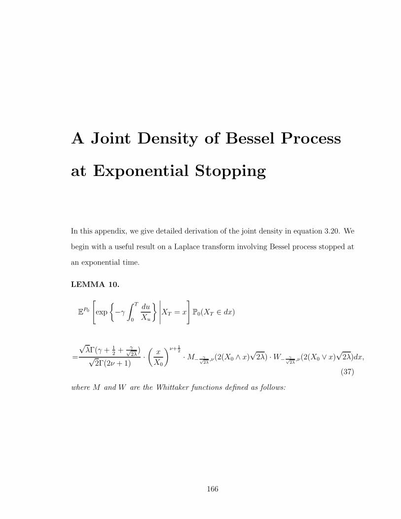
A Joint Density of Bessel Process
at Exponential Stopping
In this appendix, we give detailed derivation of the joint density in equation 3.20. We
begin with a useful result on a Laplace transform involving Bessel process stopped at
an exponential time.
LEMMA 10.
EP0
[exp
−γ
∫ T
0
du
Xu
∣∣∣∣∣XT = x
]P0(XT ∈ dx)
=
√λΓ(γ + 1
2+ γ√
2λ)
√2Γ(2ν + 1)
·(
x
X0
)ν+ 12
· M− γ√2λ
,ν(2(X0 ∧ x)√
2λ) · W− γ√2λ
,ν(2(X0 ∨ x)√
2λ)dx,
(37)
where M and W are the Whittaker functions defined as follows:
166
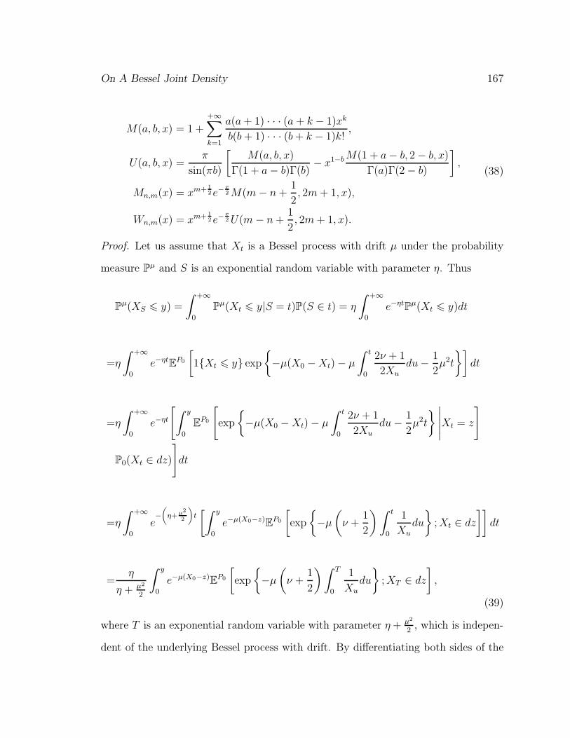
On A Bessel Joint Density 167
M(a, b, x) = 1 +
+∞∑
k=1
a(a + 1) · · · (a + k − 1)xk
b(b + 1) · · · (b + k − 1)k!,
U(a, b, x) =π
sin(πb)
[M(a, b, x)
Γ(1 + a − b)Γ(b)− x1−b M(1 + a − b, 2 − b, x)
Γ(a)Γ(2 − b)
],
Mn,m(x) = xm+ 12 e−
x2 M(m − n +
1
2, 2m + 1, x),
Wn,m(x) = xm+ 12 e−
x2 U(m − n +
1
2, 2m + 1, x).
(38)
Proof. Let us assume that Xt is a Bessel process with drift µ under the probability
measure Pµ and S is an exponential random variable with parameter η. Thus
Pµ(XS 6 y) =
∫ +∞
0
Pµ(Xt 6 y|S = t)P(S ∈ t) = η
∫ +∞
0
e−ηtPµ(Xt 6 y)dt
=η
∫ +∞
0
e−ηtEP0
[1Xt 6 y exp
−µ(X0 − Xt) − µ
∫ t
0
2ν + 1
2Xudu − 1
2µ2t
]dt
=η
∫ +∞
0
e−ηt
[∫ y
0
EP0
[exp
−µ(X0 − Xt) − µ
∫ t
0
2ν + 1
2Xudu − 1
2µ2t
∣∣∣∣∣Xt = z
]
P0(Xt ∈ dz)
]dt
=η
∫ +∞
0
e−(
η+ µ2
2
)t[∫ y
0
e−µ(X0−z)EP0
[exp
−µ
(ν +
1
2
)∫ t
0
1
Xu
du
; Xt ∈ dz
]]dt
=η
η + µ2
2
∫ y
0
e−µ(X0−z)EP0
[exp
−µ
(ν +
1
2
)∫ T
0
1
Xu
du
; XT ∈ dz
],
(39)
where T is an exponential random variable with parameter η + µ2
2, which is indepen-
dent of the underlying Bessel process with drift. By differentiating both sides of the
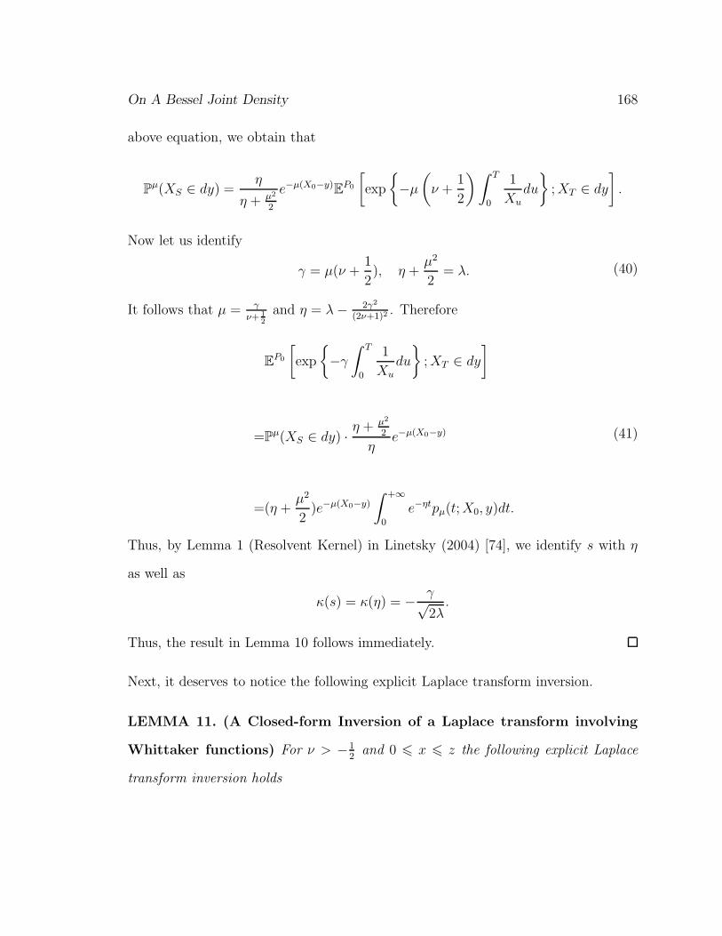
On A Bessel Joint Density 168
above equation, we obtain that
Pµ(XS ∈ dy) =η
η + µ2
2
e−µ(X0−y)EP0
[exp
−µ
(ν +
1
2
)∫ T
0
1
Xudu
; XT ∈ dy
].
Now let us identify
γ = µ(ν +1
2), η +
µ2
2= λ. (40)
It follows that µ = γ
ν+ 12
and η = λ − 2γ2
(2ν+1)2. Therefore
EP0
[exp
−γ
∫ T
0
1
Xudu
; XT ∈ dy
]
=Pµ(XS ∈ dy) · η + µ2
2
ηe−µ(X0−y)
=(η +µ2
2)e−µ(X0−y)
∫ +∞
0
e−ηtpµ(t; X0, y)dt.
(41)
Thus, by Lemma 1 (Resolvent Kernel) in Linetsky (2004) [74], we identify s with η
as well as
κ(s) = κ(η) = − γ√2λ
.
Thus, the result in Lemma 10 follows immediately.
Next, it deserves to notice the following explicit Laplace transform inversion.
LEMMA 11. (A Closed-form Inversion of a Laplace transform involving
Whittaker functions) For ν > −12
and 0 6 x 6 z the following explicit Laplace
transform inversion holds
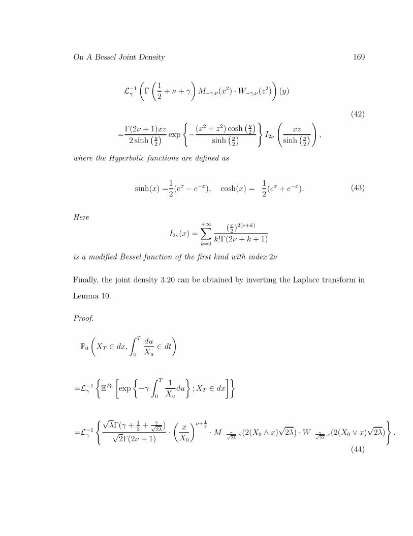
On A Bessel Joint Density 169
L−1γ
(Γ
(1
2+ ν + γ
)M−γ,ν(x
2) · W−γ,ν(z2)
)(y)
=Γ(2ν + 1)xz
2 sinh(
y2
) exp
−(x2 + z2) cosh
(y2
)
sinh(
y2
)
I2ν
(xz
sinh(
y2
))
,
(42)
where the Hyperbolic functions are defined as
sinh(x) =1
2(ex − e−x), cosh(x) =
1
2(ex + e−x). (43)
Here
I2ν(x) =
+∞∑
k=0
(x2)2(ν+k)
k!Γ(2ν + k + 1)
is a modified Bessel function of the first kind with index 2ν
Finally, the joint density 3.20 can be obtained by inverting the Laplace transform in
Lemma 10.
Proof.
P0
(XT ∈ dx,
∫ T
0
du
Xu∈ dt
)
=L−1γ
EP0
[exp
−γ
∫ T
0
1
Xudu
; XT ∈ dx
]
=L−1γ
√λΓ(γ + 1
2+ γ√
2λ)
√2Γ(2ν + 1)
·(
x
X0
)ν+ 12
· M− γ√2λ
,ν(2(X0 ∧ x)√
2λ) · W− γ√2λ
,ν(2(X0 ∨ x)√
2λ)
.
(44)

On A Bessel Joint Density 170
By using the scaling property of Laplace transform:
Lf(at)(s) =1
|a|F(s
a
),
where Lf(t)(s) = F (s). By letting a =√
2λ, we find the joint density expression
in equation 3.20.

Detailed ADI Scheme
In this appendix, we document the detailed formulation of the ADI scheme in Sec-
tion 5.2. In the implementation of (5.12), for each step n, we use a matrix Un =
(Uni,j)(I+1)×(J+1) to store the approximated values. In the first iteration of the ADI
scheme (5.12), for each fixed j ∈ 1, 2, ..., J −1 we set up an I +1 dimensional linear
system to solve for Un+ 1
2.,j . The system consists of two boundary conditions at i = 0
and i = I respectively as well as I −1 equations for inner points. The specification of
equations of inner points is straightforward. Here we need to figure out the boundary
conditions for the ADI middle step points Un+ 12 . For i = 0, it follows from the the
Dirichlet boundary condition that
Un+ 1
20,j = (1 − λA2)U
n+10,j + λA2U
n0,j = 0.
However, at i = I we operate 1 − λA2 on both sides of the Neumann boundary
condition
Un+1I,j − Un+1
I−1,j = ∆s.
Thus, we find the implied boundary condition for the ADI middle step as
Un+ 1
2I,j − U
n+ 12
I−1,j = λA2UnI,j − λA2U
nI−1,j +
(1 +
r∆t
2j∆v
)∆s.
171

Detailed ADI Scheme 172
Hence the first iteration of the ADI scheme (5.12) is translated to a tri-diagonal linear
system which can be solved efficiently by the Thomas algorithm of linear complexity.
Un+ 1
20,j = 0,
(1 − λA1)Un+ 1
21,j = [1 + A0 + (1 − λ)A1 + A2]U
n1,j ,
...
(1 − λA1)Un+ 1
2I−1,j = [1 + A0 + (1 − λ)A1 + A2]U
nI−1,j,
Un+ 1
2I,j − U
n+ 12
I−1,j = λA2UnI,j − λA2U
nI−1,j +
(1 + r∆t
2j∆v
)∆s,
(45)
i.e.
1
a1,j b1,j c1,j
. . .. . .
. . .
aI−1,j bI−1,j cI−1,j
−1 1
Un+ 1
20,j
Un+ 1
21,j
...
Un+ 1
2I−1,j
Un+ 1
2I,j
=
0
[1 + A0 + (1 − λ)A1 + A2]Un1,j
...
[1 + A0 + (1 − λ)A1 + A2]UnI−1,j
λA2UnI,j − λA2U
nI−1,j +
(1 + r∆t
2j∆v
)∆s
.
where
ai,j =λri∆t
2j∆v− λi2∆t
2, bi,j = 1 +
λr∆t
2j∆v+ λi2∆t, ci,j = −λri∆t
2j∆v− λi2∆t
2.
Similarly we handle the second iteration of the ADI scheme (5.12) as follows. We
fix i ∈ 0, 1, 2, ..., I and set up a linear equation system for solving Un+1i,. . We also
impose the boundary conditions at v = 0 and v = ∞. It follows that
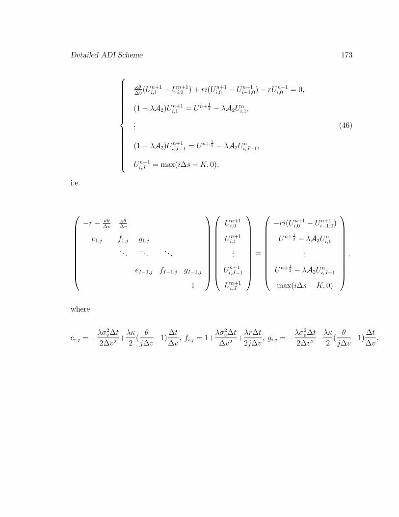
Detailed ADI Scheme 173
κθ∆v
(Un+1i,1 − Un+1
i,0 ) + ri(Un+1i,0 − Un+1
i−1,0) − rUn+1i,0 = 0,
(1 − λA2)Un+1i,1 = Un+ 1
2 − λA2Uni,1,
...
(1 − λA2)Un+1i,J−1 = Un+ 1
2 − λA2Uni,J−1,
Un+1i,J = max(i∆s − K, 0),
(46)
i.e.
−r − κθ∆v
κθ∆v
e1,j f1,j g1,j
. . .. . .
. . .
eI−1,j fI−1,j gI−1,j
1
Un+1i,0
Un+1i,1
...
Un+1i,J−1
Un+1i,J
=
−ri(Un+1i,0 − Un+1
i−1,0)
Un+ 12 − λA2U
ni,1
...
Un+ 12 − λA2U
ni,J−1
max(i∆s − K, 0)
,
where
ei,j = −λσ2v∆t
2∆v2+
λκ
2(
θ
j∆v−1)
∆t
∆v, fi,j = 1+
λσ2v∆t
∆v2+
λr∆t
2j∆v, gi,j = −λσ2
v∆t
2∆v2−λκ
2(
θ
j∆v−1)
∆t
∆v.
Consideration of Jump Combined
with Stochastic Volatility
In this appendix, we outline some ideas on pricing timer call options under stochastic
volatility models with jumps (see Bates [4] and Duffie, Pan and Singleton [37]). Unlike
the case of Heston’s model, the stochastic volatility with jump models might not
render semi-closed form formulae for the valuation of timer options. However, we
may still propose a conditional Black-Scholes-Merton formula and implement it via
Monte Carlo simulation.
Under the risk neutral probability measure, Bates’ [4] stochastic volatility with jump
model is specified as
dSt
St−= (r − λµ)dt +
√Vt(ρdW
(1)t +
√1 − ρ2dW
(2)t ) + d
[Nt∑
i=1
(ξsi − 1)
],
dVt = κ(θ − Vt)dt + σv
√VtdW
(1)t ,
(47)
where (W (1)t , W
(2)t ) is a two dimensional standard Brownian motion; r is assumed
to be the constant instantaneous interest rate; Nt is a Poisson process with constant
intensity λ; ξsi is the relative jump size in the stock price. At time ti, when jump
174
Jump SV and Timer Option 175
occurs, we have that
Sti = Sti−ξsi .
Let us assume that ξs follows a lognormal distribution with mean µs and variance σ2s ,
i.e.
ξs ∼ LN (µs, σ2s).
Because
µ = Eξsi − 1 = Eeµs+σsZ − 1,
where Z ∼ N (0, 1), the parameter µs and µ are related to each other by the equation
µs = log(1 + µ) − 1
2σ2
s .
Under Bates’ model (47), the theoretical realized variance consists of not only the
diffusion part but also the compounded Poisson part (see Carr and Wu (2006) [22]).
PROPOSITION 16. Under Bates’ model (47), we have that, for t = m∆t,
lim∆t→0
m∑
j=1
(log
Stj
Stj−1
)2
= IJt :=
∫ t
0
Vsds +Nt∑
i=1
[log(ξsi )]
2 , a.s. (48)
In the continuous-time setting, we consider the first-passage-time:
τJ =
u ≥ 0,
∫ u
0
Vsds +Nt∑
i=1
[log(ξsi )]
2 > B
. (49)
Let us denote
To = IJτ − B =
∫ τJ
0
Vsds +
NτJ∑
i=1
[log(ξsi )]
2 − B (50)

Jump SV and Timer Option 176
the size of overshoot over the variance budget B by the total variance. Similar to
Proposition 3, we have the following conditional Black-Scholes-Merton formula for
pricing timer options under Bates’ stochastic volatility with jump model.
PROPOSITION 17. The timer call option with strike K and variance budget B
can be priced by the following conditional Black-Scholes-Merton formula:
C0 =EQ
[S0
NτJ∏
i=1
ξsi · ed0(V
τJ ,τJ ,∑N
τJ
i=1 [log(ξsi )]
2,To)N(d1(VτJ , τJ ,
NτJ∑
i=1
[log(ξsi )]
2 , To))
− Ke−rτJ
N(d2(VτJ , τJ ,
NτJ∑
i=1
[log(ξsi )]
2 , To))
],
(51)
where
N(x) =1√2π
∫ x
−∞e−
u2
2 du,
and
d0(v, ξ, p, q) =ρ
σv(v − V0 − κθξ + κ(B − p + q)) − 1
2ρ2(B − p + q),
d1(v, ξ, p, q) =1√
(1 − ρ2)(B − p + q)
[log
(S0
K
)+ rξ +
1
2(B − p + q)(1 − ρ2) + d0(v, ξ, p, q)
],
d2(v, ξ, p, q) =1√
(1 − ρ2)(B − p + q)
[log
(S0
K
)+ rξ − 1
2(B − p + q)(1 − ρ2) + d0(v, ξ, p, q)
].
(52)
Proof. First, we express (St, Vt) as
St = S0 exp
rt − 1
2
∫ t
0
Vsds + ρ
∫ t
0
√VsdW (1)
s +√
1 − ρ2
∫ t
0
√VsdW (2)
s
Nt∏
i=1
ξsi ,
Vt = V0 + κθt − κ
∫ t
0
Vsds + σv
∫ t
0
√VsdW (1)
s .
(53)
By conditioning on the variance budget consumption time τJ , the variance VτJ , the
total number of Poisson jumps NτJ , the jump sizes (ξsi )
NτJ
i=1 , the total quadratic varia-

Jump SV and Timer Option 177
tion contributed by jumps∑N
τJ
i=1 [log(ξsi )]
2 and the overshoot size of the total variation
To, we find the conditional distribution of SτJ . We note that all the conditions are
based on the variance process and the jump part of the asset dynamics, which are
both independent of the Brownian motion W(1)t . Similar argument to the proof of
Proposition 3 yields that
SτJ
∣∣∣∣∣τJ = t, VτJ = v, NτJ = n, (ξs
i )N
τJ
i=1 = (ξi)ni=1 ,
NτJ∑
i=1
[log(ξsi )]
2 = p, To = q
=law
(S0
Nt∏
i=1
ξsi exp
rτJ − 1
2(B − p + q) +
ρ
σv
(VτJ − V0 − κθτJ + κ(B − p + q))
+√
1 − ρ2
∫ τJ
0
√VsdW (2)
s
∣∣∣∣∣τJ = t, VτJ = v, NτJ = n, (ξs
i )N
τJ
i=1 = (ξi)ni=1 ,
NτJ∑
i=1
[log(ξsi )]
2 = p, To = q
)
=lawS0
n∏
i=1
ξi exp
N
(rt − 1
2(B − p + q) +
ρ
σv
(v − V0 − κθt + κ(B − p + q)),
(1 − ρ2)(B − p + q)
).
(54)
Therefore, by conditioning and further computation based on the standard normal
distribution, we obtain that
C0 =EQ
EQ
e−rτJ
max(SτJ − K, 0)
∣∣∣∣∣(ξsi )
NτJ
i=1 , NτJ , τJ , VτJ ,
NτJ∑
i=1
[log(ξsi )]
2 , To
=EQ
[S0
NτJ∏
i=1
ξsi · ed0(V
τJ ,τJ ,∑N
τJ
i=1 [log(ξsi )]
2,To)N(d1(VτJ , τJ ,
NτJ∑
i=1
[log(ξsi )]
2 , To))
− Ke−rτJ
N(d2(VτJ , τJ ,
NτJ∑
i=1
[log(ξsi )]
2 , To))
].
(55)

Jump SV and Timer Option 178
A conditional Monte Carlo simulation scheme can be implemented based on Propo-
sition 17. Similar to Algorithm 1, we perform the exact simulation of the path
of variance process Vt and the jump components in (48). By the definition of
τJ in (49), we simulate it by a “time-checking” algorithm (see 1). Meanwhile, we
record the size of overshoot To and the quadratic variation contributed by jumps, i.e.∑N
τJ
i=1 [log(ξsi )]
2 . Based on all these steps, we calculate the estimator:
S0
NτJ∏
i=1
ξsi · ed0N(d1) − Ke−rτJ
N(d2), (56)
where d0, d1, d2 are evaluated as in Proposition 17.

The Malliavin-Watanabe-Yoshida
Theory: A Primer
In recent years, various researches on the applications of Malliavin calculus in quan-
titative finance are vividly carried out. For example, Fournie et al. (1999) [45] pro-
posed to use Malliavin integration by parts formula to derive Monte Carlo simulation
estimator for computing price sensitivities. Among many other applications, Malli-
avin calculus provides researchers a powerful tool to justify asymptotic expansion of
derivative security payoffs and thus its no-arbitrage price approximation. Some ex-
amples applied to interest rates modeling can be found in Kunitomo and Takahashi
(2001) [70] and Osajima (2007) [82], etc. More topics on the applications of Malliavin
calculus in finance can be found in Malliavin and Thalmaier (2006) [78].
.1 Basic Setup of the Malliavin Calculus Theory
The Malliavin calculus, also known as the stochastic calculus of variations, is an
infinite-dimensional differential calculus on the Wiener space. It was originally tai-
lored to investigate regularity properties of the law of Wiener functionals such as
solutions of stochastic differential equations. The theory was initiated by Malliavin
179

The Malliavin-Watanabe-Yoshida Theory 180
and further developed by Stroock, Bismut, Watanabe, et al. Roughly speaking, the
Malliavin calculus theory consists of two parts. First is the theory of the differen-
tial operators defined on Sobolev spaces of Wiener functionals. The second part of
the theory establishes general criteria for a given random vector to possess a smooth
density.
Instead of making an exhaustive survey of the Malliavin calculus theory, we briefly
list some terminologies related to the asymptotic expansion theory of Malliavin-
Watanabe-Yoshida. To learn more about the fundamentals of Malliavin calculus,
readers are referred to Nualart (2006) [80], Malliavin (1997) [77], Kusuoka and Stroock
(1991) [72] and Fritz (2005) [46], etc.
Let us denote (Ω, P,F , Ft) the d-dimensional filtered Wiener space, where Ω =
C0([0, T ],Rd). The coordinate process w(t) is a d-dimensional Brownian motion
under the Wiener measure P. Let H be the Cameron-Martin subspace of Ω, i.e.
H =
h =
(∫ ·
0
h1(s)ds, ...,
∫ ·
0
hd(s)ds
); h ∈ L2[0, T ]
.
The inner product of Hilbert space H is defined as
〈h1, h2〉H =d∑
k=1
∫ T
0
hk1(s)h
k2(s)ds,
for any h1, h2 ∈ H. The norm is equipped with
||h||H =
(d∑
k=1
∫ T
0
|hk(t)|2dt
) 12
,
for h ∈ H. Let F : Ω → R be an FT measurable random variable, which is also called
Wiener functional. We further assume that F ∈ Lp(Ω), where p > 1. Given h ∈ H ,

The Malliavin-Watanabe-Yoshida Theory 181
we define the directional derivative of F as
DhF (w) :=d
dǫ
∣∣∣∣ǫ=0
F (w + ǫh) = limǫ→0
1
ǫ[F (w + ǫh) − F (w)] . (57)
Thus, D·F (w) is defined as a linear functional on Hilbert space H . By Riesz represen-
tation theory, there exists an element DsF (w) := (D1F (w), D2F (w), ..., DdF (w)) ∈
H such that
DhF (w) = 〈h, DF (w)〉H =d∑
k=1
∫ T
0
hk(s)DksF (w)ds. (58)
Denote Lp(Ω : H) the collection of measurable map f from Ω to H such that
||f ||H ∈ Lp(Ω). If DF ∈ Lp(Ω : H), DF is defined as the Malliavin derivative
of F . It can be regarded as an H-valued random variable or a d-dimensional stochas-
tic process. Consequently we are able to define higher order Malliavin derivatives.
Let P denote the collection of polynomials on the Wiener space Ω. Let us define the
s-times Malliavin norm || · ||s,p as
‖F‖s,p =
[E‖F‖p +
s∑
j=1
E‖D(j)F‖pH⊗j
] 1p
. (59)
By completing P (in Lp(Ω)) according to norm || · ||s,p, we construct a Banach space
denoted by Dsp, which collects all s-times Malliavin differentiable variables.
It is well known that, for s ∈ N, norm (59) is equivalent to the one defined as follows.
For any Wiener functional g, let
|||g|||s,p =‖ (I − L)s2 g ‖Lp(Ω), (60)
where L is the Ornstein-Uhlenbeck operator. However, using norm (60), we can obtain
The Malliavin-Watanabe-Yoshida Theory 182
space Dsp for any arbitrary real number s ∈ R by completing the Wiener polynomial
space P. For any s ∈ N, the equivalence ensures that the completion using norm
||| · |||s,p also generates the space Dsp. It is well known that the dual space of Ds
p is
D−sq , i.e. (Ds
p)′ = D−s
q , where
1
p+
1
q= 1.
If s < 0 the elements in Dsp may not be ordinary random variables and they are
usually interpreted as distributions on the Wiener space. If F ∈ Dsp and G ∈ D−s
q ,
we denote the paring 〈F, G〉 by E(FG). Thus, we interpret norm || · ||−s,q as
||G||−s,q = sup E(FG),
where the sup is taken over set
F ∈ Dsp : ||F ||s,p < 1.
Consider the intersection
D∞ :=⋂
p>1
⋂
k>1
Dkp , D−∞ :=
⋂
p>1
⋃
k>1
D−kp .
Here, D∞ is the set of Wiener functionals. D−∞ is the set of generalized Wiener
functionals.
The original motivation of the Malliavin calculus theory has been to give a proba-
bilistic proof of Hormander’s “sum of squares” theorem. The key task in this regard
is to establish general criteria in terms of the Malliavin covariance matrix for a given
random vector to possess a smooth density. In the applications of Malliavin calculus
to specific examples, one usually tries to find sufficient conditions for these general cri-

The Malliavin-Watanabe-Yoshida Theory 183
teria to be satisfied. To apply the Malliavin-Watanabe-Yoshida thoery of asymptotic
expansion, it is crucial for us to justify the validity through the Malliavin covariance
of the underlying variables.
Let G be a m-dimensional random variable G = (G1, G2, ..., Gm) and denote
DG = (DjGi)m×d,
which appears as a m×d-matrix of H-valued random variable. The Malliavin covari-
ance matrix is defined as
Σ(G) = (Σ(G)ij)m×m, (61)
where
Σ(G)ij = 〈DGi, DGj〉H =d∑
k=1
〈DkGi, DkGj〉H .
REMARK 15. The analog of Malliavin derivative operator in finite dimensional
space Rn is the gradient operator. Given a C1-function f : Rn → R, the derivative
along direction −→n can be computed as
∂f
∂−→n = ∇f · −→n .
The resemblance to (58) convinces us that the Malliavin calculus generalizes the
ordinary finite dimensional calculus to infinite dimensional settings. For more such
analogies between the Malliavin calculus and the ordinary finite dimensional calculus,
see Friz (2002) [46].

The Malliavin-Watanabe-Yoshida Theory 184
.2 The Malliavin-Watanabe-Yoshida Theory of Asymp-
totic Expansion
Suppose the random variable G(ǫ) admits the asymptotic expansion in D∞, i.e.
G(ǫ) = G0 + ǫG1 + ǫ2G2 + · · · + ǫnGn + O(ǫn+1), in D∞. (62)
In other words,
lim supǫ→0
1
ǫn+1
∥∥G(ǫ)− [G0 + ǫG1 + ǫ2G2 + · · ·+ ǫnGn]∥∥
Dsp< +∞, for any p > 1, s > 0,
(63)
where Gi ∈ D∞ for i = 0, 1, 2, 3, ....
Let S be the real Schwartz space of rapidly decreasing C∞-functions. Denote S ′ the
space of Schwartz tempered distribution, which is the dual space of S. Now, for
T ∈ S ′, the question is under what condition we have that
E[T (G(ǫ))] = EΦ0 + ǫEΦ1 + ǫ2EΦ2 + · · · + ǫnEΦn + O(ǫn+1), (64)
where
Φ0 = T (G0), Φ1 =∂T
∂x(G0)G1, Φ2 =
1
2
∂2T
∂x2(G0)G
21 +
∂T
∂x(G0)G2, ... . (65)
It is sufficient to answer under what condition we have the asymptotic expansion for
generalized Wiener functional T (G(ǫ)), i.e.
T (G(ǫ)) = Φ0 + ǫΦ1 + ǫ2Φ2 + · · · + ǫnΦn + O(ǫn+1), in D−∞. (66)

The Malliavin-Watanabe-Yoshida Theory 185
In other words, there exists s > 0 such that, for all p > 1
lim supǫ→0
1
ǫn+1
∥∥T (G(ǫ)) − [Φ0 + ǫΦ1 + ǫ2Φ2 + · · · + ǫnΦn]∥∥
D−sp
< +∞, (67)
where Φi ∈ D−sp , for i = 0, 1, 2, 3, ... .
Watanabe (1987) successfully interpreted the composition functional T (G(ǫ)) as gen-
eralized Wiener functionals (i.e. the Schwartz distribution on the probability space.)
He justified that the asymptotic expansion in (66) and (64) is valid if the Malliavin
covariance of G(ǫ) is uniformly non-degenerated in the sense that
lim supǫ→0
E[det(Σ(G(ǫ)))−p] < ∞, for all p ∈ (0, +∞). (68)
A crucial step to apply this successful theory is to verify the non-degeneracy of the
Malliavin covariance. This is even not easy to do for some simple cases where the
underlying Malliavin covariance is expressed by an integration of some adaptive pro-
cesses. Yoshida (1992, 1993) [93, 92, 94] not only successfully applies the theory to
statistical inference, but also gives a truncated version of the asymptotic expansion
theory, in which verification of the uniform non-degeneracy of Malliavin covariance
becomes easier. According to Yoshida (1992, 1993) [93, 92, 94], the validity of the
expansion can be obtained if there exists a random sequence ηǫ j D∞ such that
the following two conditions are verified.
Condition.1: Uniform Non-degeneracy under Truncation
supǫ∈[0,1]
E[1ηǫ ≤ 1(det(Σ(G(ǫ))))−p] < +∞; (69)
The Malliavin-Watanabe-Yoshida Theory 186
Condition.2: Negligible Probability of Truncation
limǫ→0
1
ǫnP
(|ηǫ| >
1
2
)= 0, for any n = 1, 2, 3, ... (70)
By reasonably modifying Watanabe (1987), Yoshida (1992, 1993) [93, 92, 94] es-
tablishes that the generalized Wiener functional Ψ(ηǫ)T (G(ǫ)) admits the following
expansion
Ψ(ηǫ)T (G(ǫ)) = Φ0 + ǫΦ1 + ǫ2Φ2 + · · ·, in D−∞, (71)
where Ψ : R → R is a smooth function such that 0 ≤ Ψ(x) ≤ 1 for x ∈ R,
Ψ(x) = 1, for |x| < 1/2 and Ψ(x) = 0, for |x| ≥ 1. Thus, (64) follows directly.
Interested readers are also referred to Uchida and Yoshida (2004) [89], Kunitomo
and Takahashi (2001) [70, 71] for the development and application of the Malliavin-
Watanabe-Yoshida theory in the valuation of contingent claims.


