1
Mapping and Economic Development: Spatial Information Matters1
Dongwoo Yoo, West Virginia University
Abstract: Maps, which record spatial information, are critical for all human activities. This
paper aims to evaluate the impact of mapping on economic development. Military leaders need
maps for the planning and execution of movement, combat, accommodation and supply. Thus,
maps have long been considered as military secrets. However, mapping was also critical for
civilian and cadastral (i.e. land tax) purposes. After realizing the value of maps for land taxation,
European countries collected more geodetic data for cadastral purposes and linked those data to
military topographic maps. In sharp contrast, the principle of military secrecy in mapping still
pervades in many developing countries to this day. In most Latin American countries, the
military forces hold the legislated national monopoly of mapping services. The military is able to
help finance itself by charging rather high prices for its mapping services. Many cases across the
world suggest that mapping, especially cadastral mapping, is critical for economic development.
Empirical estimates using introduction of triangulation and cadastral survey as instruments
suggest that mapping is an important institutional foundation of economic development.
[VERY ROUGH DRAFT]
1 This Research Project is supported by 2014 Joint Usage and Research Center Project, Hitotsubashi University,
IERPK1412.

2
1. Introduction
Maps, which record spatial information, are critical for all human activities throughout
the history. The cartographer’s rule is simple: “you may have no data without a map” (Mugnier,
Nov. 2001).
The major initiative of “large scale” mapping was wars. The efficiency of wars
significantly improves with a map. Military leaders need maps for the planning and execution of
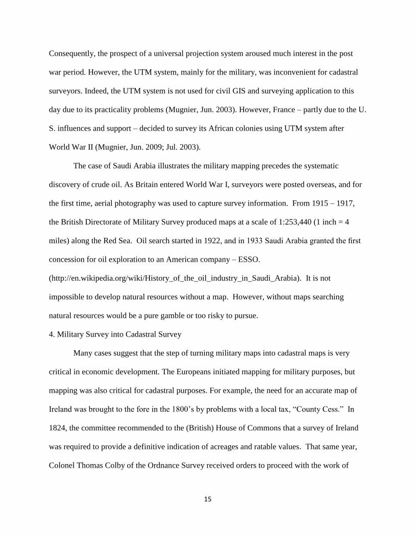
movement, combat, accommodation and supply. Topographic maps (which focus on contour
lines, figure 1) were very valuable for the military; thus considered as military secrets. For
example, Napoleon Bonaparte produced maps of Europe, but afterwards the French had kept
military maps as military secrets. Printing large numbers of copies was considered too dangerous
(Mugnier, Nov. 2001). As a matter of fact, the military secrecy still remains to this day. Global
Positioning System (GPS) is provided by American military satellites. Until May 2000, there
was a policy called Selective Availability (SA): an intentional degradation of public GPS signals
implemented for national security reasons. Still now, military GPS is more accurate than civilian
GPS (http://www.gps.gov/systems/gps/performance/accuracy/).
The Europeans initiated mapping for military purposes, but mapping was also critical for
civilian and cadastral (i.e. land tax) purposes. Generally, the topography was of more interest to
the soldier than to the tax collector, and measuring accurate boundaries and area of plots was of
more interest to the tax collector than to the soldier (figure 2). However, before the introduction
of satellites, large scale mapping was much more difficult than one can imagine (even with GPS
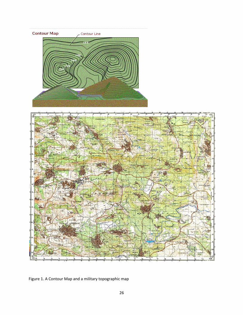
technologies, making cadastral maps are not a simple task). Triangulation (i. e. the process of
determining the location of a point by measuring angles to it from known points at either end of a

3
fixed baseline, figure 3) is the best way of measuring the area and distance, but accurate
triangulation requires a lot of mathematical and technological knowledge.
This paper aims to evaluate the impact of mapping on economic development. To my
best knowledge, there is no prior research on mapping and economic development. A history of
mapping clearly suggests that the efficiency of economic activities significantly improves after
mapping. However, it is also possible that good mapping can be a result of economic
development. In other words, a government maps developed area first, and expands mapping to
rural areas (or neglects mapping in the rural areas). To address this endogeneity issue, this paper
focuses on the modern large scale mapping technique, triangulation. When cartographers are
making cadastral maps with triangulation, large scale maps are produced first, and then small
scale maps are produced referring the large scale maps. Technical procedures of triangulation
suggest that the endogeneity problem is not very severe in mapping.
After realizing the value of maps for land taxation, European countries produced
cadastral maps for entire countries. The secrecy of mapping became obsolete and maps can be
used for civilian purposes with few restrictions. Surprisingly, the principle of military secrecy in
mapping still remains in many developing countries. In most Latin American countries, the
military have the legislated national monopoly of mapping. Indeed, the military finances itself by
selling maps at high prices (Mugnier, Nov. 2001). The secrecy of mapping discouraged the
development of civilian and cadastral mapping, and the development of property rights
institutions in land.
Many cases across the world suggest that mapping, especially cadastral mapping, is
critical for economic development. For example, Poland was occupied by Prussia, Austria, and
Russia. The Prussians and the Austrians introduced cadastral mapping. However, the Russians

4
introduced only military mapping during the 19th and early 20th centuries (Mugnier, Sep. 2000).
Nowadays, one can observe that the level of economic development is lower in the areas that
occupied by the Russia.
This paper assumes that the accurate mapping is an important institutional foundation of
economic development. Many cases across the world suggest that cadastral maps were more
critical for economic development because it is directly related to 1) government’s finance
through land registration and taxation systems; 2) land transactions; 3) land collateralizations.
However, making cadastral maps or turning military maps into cadastral maps is very costly
(Similarly, turning google maps into cadastral maps is not a simple task, and most governments
still rely on traditional cadastral maps to identify boundaries). Consequently, different colonizers
and governments made different decisions, which impacted the development of property rights
institutions and economic development. Empirical estimates using introduction of triangulation
as a major instrument suggest that mapping is an important institutional foundation of economic
development.
Section 2 provides theoretical motivations. Section 3 describes mapping techniques.
Section 4 discusses endogeneity issues between mapping and economic development. Section 5
describes military secrecy in mapping. Section 6 describes how mapping affects other factors of
production. Section 7 provides empirical estimates. Section 8 concludes.
2. Theoretical Motivation
This section provides a theoretical motivation based on neoclassical (Solow) growth
model. The model assumes that institutions may increase output (per capita) through a variety of
ways, including more effective land use, physical capital formation, human resource
management, and higher productivity. For example, assume that two countries have the same
amount of available land, population, capital, and technology. However, a country with an

5
efficient land markets (based on better mapping and land tenure systems) has more effective
amount of land supply compared to another country with inefficient land markets. It is also
reasonable to assume that saving rate is higher for a country with secure financial institutions
(based on efficient land collateralization) compared to another country with insecure financial
institutions. Similarly, secure financial market also facilitates the invention and transfer of new
technologies. Finally, the factors that impacts productivity – for example, transportation and city
planning - can be more efficiently organized with better spatial information.
It is worth to note that some legal historians observe that “secure property rights in land
established a precedent for the establishment of secure property rights in general (Hughes and
Cain 2011).” Indeed, property rights institutions in land provided basic structure of other
institutions. For example, land collateralization is directly related the financial markets. The
patent law which defines property rights in an imaginary space of knowledge refers a lot in
property law in land (which defines property rights in a real space). Finally, citizen identification
system – that is required for the government to identify the owner (and the tax payer) from the
land register – provides a basic frame of population management system (however, the link
between mapping and human capital is relative weak, thus in the empirical estimation, education
is controlled additionally).
Following Acemoglu and Johnson (2007), I assume economy i has an aggregate
production function:
(1)
where, denotes technology, denotes the effective units of labor, denotes capital, and
denotes the effective supply of land.

6
To capture the effects of mapping in a reduced form manner, the model assumes the
following relationships:
(2)
,
(3)
,
(4)
where is institutional quality in country i at time t, is total population, is human
capital per person, is quality of property rights in land, and is territory of country i. , and
, , and denote the baseline differences across countries.
These equations illustrate that the technology, human capital, and effective land supply
adjust as institutions change, although land may be inelastically supplied in the long run without
territorial expansion.
The evolution of capital stock in country i at time t is given by
,
where denotes saving rates in country i at time t, is capital depreciation rate, and denotes
the baseline differences across countries.
To analyze the impact of institutions in a simple way, the model assumes that after
technology, human capital, land supply, and saving rate have adjusted, the steady-state capital
stock level will be
(6)
In this case, substituting (2) – (6) into (1) and taking logs, I obtain the following log-
linear relationship between log institutional quality, , and log income per capita,
:

7
In the estimation equation, I assume that the country characteristics affect factors of
production through institutions. In other words, I assume that the country specific parameters ,
,
, and, are common across all countries when institutional quality is controlled.
The estimation equation (7) also can be written as
This equation suggests that log population density affects log income per capita.
However, there exists endogeneity between log income per capita and institutional quality. To
make it a causal relationship, I need excluded exogenous variables for institutional quality.
where denotes excluded exogenous variables (This paper uses the quality of mapping,
especially, the introduction of triangulation and cadastral mapping as major instruments).
Interestingly, the equation (8) shows that current log population density can be used as
included exogenous variable in the first stage (equation (9)), assuming that equation (3) and (4)
isolate endogeneity between human capital, effective land supply, and log income per capita (In
8
empirical estimation, other variables such as education, saving rates, and population density are
assumed to be endogenous in some specifications).
Or, it might be possible to use lagged value of , , and
as included instruments,
assuming that , , and
are not common across all countries ( is assumed to be common
across all countries and this is measures by a constant).
where denotes lagged value of productivity, human capital and savings rates.
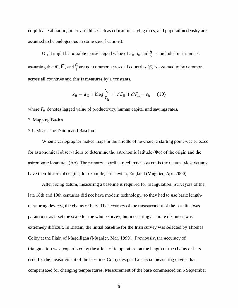
3. Mapping Basics
3.1. Measuring Datum and Baseline
When a cartographer makes maps in the middle of nowhere, a starting point was selected
for astronomical observations to determine the astronomic latitude (Φo) of the origin and the
astronomic longitude (Λo). The primary coordinate reference system is the datum. Most datums
have their historical origins, for example, Greenwich, England (Mugnier, Apr. 2000).
After fixing datum, measuring a baseline is required for triangulation. Surveyors of the
late 18th and 19th centuries did not have modern technology, so they had to use basic length-
measuring devices, the chains or bars. The accuracy of the measurement of the baseline was
paramount as it set the scale for the whole survey, but measuring accurate distances was
extremely difficult. In Britain, the initial baseline for the Irish survey was selected by Thomas
Colby at the Plain of Magelligan (Mugnier, Mar. 1999). Previously, the accuracy of
triangulation was jeopardized by the affect of temperature on the length of the chains or bars
used for the measurement of the baseline. Colby designed a special measuring device that
compensated for changing temperatures. Measurement of the base commenced on 6 September
9
1827 with 70 men and was completed on 20 November 1828. The length of the base, leveled and
reduced to the adjoining sea level, was 41,640.8873 feet or nearly 8 miles.2
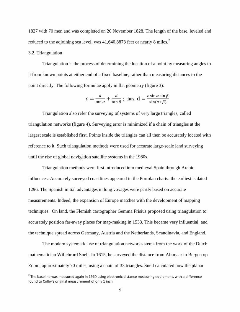
3.2. Triangulation
Triangulation is the process of determining the location of a point by measuring angles to
it from known points at either end of a fixed baseline, rather than measuring distances to the
point directly. The following formulae apply in flat geometry (figure 3):
; thus,
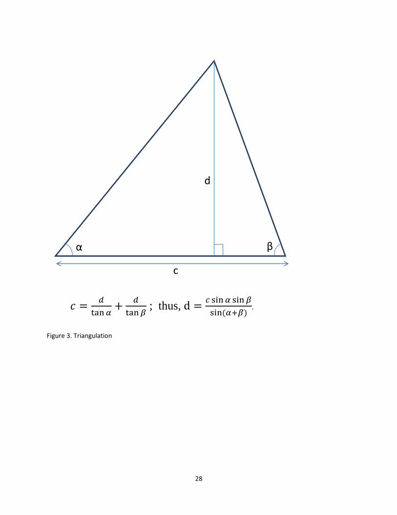
Triangulation also refer the surveying of systems of very large triangles, called
triangulation networks (figure 4). Surveying error is minimized if a chain of triangles at the
largest scale is established first. Points inside the triangles can all then be accurately located with
reference to it. Such triangulation methods were used for accurate large-scale land surveying
until the rise of global navigation satellite systems in the 1980s.
Triangulation methods were first introduced into medieval Spain through Arabic
influences. Accurately surveyed coastlines appeared in the Portolan charts: the earliest is dated
1296. The Spanish initial advantages in long voyages were partly based on accurate
measurements. Indeed, the expansion of Europe matches with the development of mapping
techniques. On land, the Flemish cartographer Gemma Frisius proposed using triangulation to
accurately position far-away places for map-making in 1533. This became very influential, and
the technique spread across Germany, Austria and the Netherlands, Scandinavia, and England.
The modern systematic use of triangulation networks stems from the work of the Dutch
mathematician Willebrord Snell. In 1615, he surveyed the distance from Alkmaar to Bergen op
Zoom, approximately 70 miles, using a chain of 33 triangles. Snell calculated how the planar
2 The baseline was measured again in 1960 using electronic distance measuring equipment, with a difference
found to Colby’s original measurement of only 1 inch.

10
formulae could be corrected to allow for the curvature of the earth. He also showed “how to
resection (figure 5), or calculate, the position of a point inside a triangle using the angles cast
between the vertices at the unknown point. These could be measured much more accurately than
bearings of the vertices, which depended on a compass.” This established the key idea of
surveying a large-scale primary network of control points first, and then locating secondary
subsidiary points later, within that primary network (figure 6 and 7).
In the end of the 18th century that European countries began to establish detailed
triangulation network surveys to map whole countries. The Principal Triangulation of Great
Britain was begun by the Ordnance Survey in 1783. For the Napoleonic French state, the French
triangulation was extended by Jean Joseph Tranchot into the German Rhineland from 1801,
subsequently completed after 1815 by the Prussian general Karl von Müffling. Meanwhile, the
famous mathematician Carl Friedrich Gauss was entrusted from 1821 to 1825 with the
triangulation of the kingdom of Hanover, for which he developed the method of least squares to
find the best fit solution for problems of large systems of simultaneous equations given more
real-world measurements than unknowns (http://en.wikipedia.org/wiki/Triangulation).
3.3. Scaling factors and GPS systems
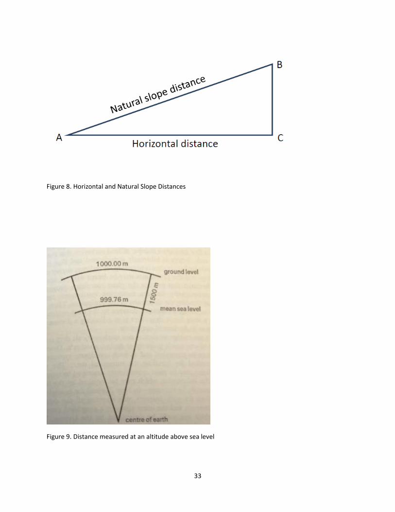
Mapping is a projection (or a mathematical transformation) from measurements on the
curved surface of Earth to measures on a plane; In all numerical systems, for describing the
location of boundaries, measurement of distance refer the horizontal straight line distance
between points (points A and C in figure 8). This distance, is shorter than any slope distance
which may be measured (points A and B in figure 8) and hence must be derived from the slope
distance which may by applying what surveyors called a ‘correction’ to the measured value.
Similarly when distances are measured at altitude, the nominal length will be longer than the

11
equivalent value that would have occurred at mean sea level. For example, a distance of 1000m
at an altitude of 1500m is equivalent to a distance of 999.76 m at mean sea level, because of the
curvature of the Earth (figure 9). Thus, the distance between two points computed on a map
projection system is not consistent with the value measured on the ground; the difference
between the two values is a matter of scale and the ratio between them is called the scale factor
(Dale 1976). [For more practical difficulties in mapping in developing countries, please refer the
appendix.]
Furthermore, even with the GPS system, making cadastral maps is not a simple task.
Although a GPS-controlled project is largely free of systematic error when properly executed,
the prospect of quantifying the systematic error of an older data set and incorporating that older
data into the new system can be daunting (for example see figure 10. It is possible to overlap an
traditional map onto modern maps, but the accuracy is not easily guaranteed. In addition
overlapping is possible when a government has traditional cadastral maps). A successful
mapping project depends on the merging of the old with the new. An understanding and
knowledge of past practices, techniques, and reference systems is the pre-requisite to that success
(Mugnier, Nov. 2003). For example, land surveyors in Palau informed me that the American
land survey results with GPS technology are not yet compatible with the Japanese triangulation
land survey results, partly due to different scaling factors.
4. Endogeneity issues in mapping
The paper assumes that accurate mapping is an important institutional foundation of
economic development. Many developing countries did not or still do not have reliable maps.
For example, there had never been a general map of Bolivia until 1921. Sketch maps were
virtually the only maps available of Guatemala by 1930. El Salvador became independent in
12
1821, but until 1930 the only detailed accurate mapping was the surveying done for the
Intercontinental Railroad Commission (Mugnier, Dec. 2000; Jul. 2008; Jul 2005).
However, it is also possible that the accurate mapping is the result of economic
development. The review of mapping techniques, however, suggests that this endogeneity issue
may not be very critical in modern mapping, especially when triangulation is used. The demand
for mapping is larger in urban (or developed) areas. Thus, one may suspect that a government
maps urban (or developed) areas first and then expands the mapping to rural areas (or the
government neglects rural areas in mapping). This could be true in traditional map making
without triangulation. However, with triangulation, large a scale primary network is established
first and then establishes secondary networks later, within the primary network. For example, in
Korea 400 primary stations, 2,401 second-order stations, and 31,646 third-order triangulation
stations were established sequentially. In other words, triangulation produces large scale maps
first, and then produces small scale maps referring large scale maps. This suggests that mapping
urban (or developed) areas first and then expands (or neglects) rural mapping is not an optimal
strategy. Indeed, urban mapping requires more accuracy and surveying error is minimized if a
chain of triangles at the largest appropriate scale is established first. Consequently, ignoring
accuracy of primary and secondary networks in rural area is not recommended in triangulation.
Indeed, in Cyprus, the triangulation was not accurate enough in urban areas, thus the government
measured baseline, and other triangulation networks again.
Moreover, before World War I, the lay of the land to be mapped was largely unknown.
Photogrammetry (i. e. taking pictures from airplanes) was first introduced during World War I.
Thus, there was little opportunity to plan where surveying control would be established and
mapping could proceed. No graticules (i.e. the grid of intersecting lines, especially of latitude

13
and longitude) were prepared in advance. The manuscripts had to be prepared first at the base
camp in a tent. With prior knowledge of what and where mapping was to be accomplished, the
efficiency of mapping increases significantly (Mugnier, Sep. 1997). However, before
photogrammetry, attaining prior knowledge was practically impossible, suggesting that the
proceeding direction of mapping is exogenous to economic potentials. For example, when
Britain planned to map its African colonies before World War I, the British had “no data” on
where to proceed mapping. The British proceeded to map Africa following the line of ‘30th
Meridian East of Greenwich’ which seems to be exogenous to the economic potential (figure 11).
The Arc of the 30th
meridian was proposed as the foundation of triangulation in the East African
colonies, but the British was not able to complete the survey.
Mars also provides a good example that suggests that making a map may not related to
the level of economic development or economic potential. Making a map of Mars is one of the
most important projects of NASA because all activities require the map. In other words, NASA
is making the map not because of high level of economic development (or potential) of Mars, but
because collecting, recording and processing data require the map. Currently, NASA is
struggling with making a map in Mars because the principles on ‘geodetic controls of the earth’
are not directly applicable to Mars. For example, measuring the latitude and the longitude in
Mars is not very accurate because cartographers do not have a fixed point and cannot observe
stars accurately (Mugnier, Oct. 2005). It is clear that improved mapping technologies in Mars
will facilitate all activities through accurate maps.
It may be possible to manage small scale development without a map (just like winning a
small scale battle without a map is possible). However, the efficiency of large scale development
will be significantly improved if the planners have correct spatial information. Also, it is

14
impossible to imagine to build up national highways, railroads or pipelines without maps. For
example, Russian government asked Marathon to design, construct and build a pipeline from the
offshore petroleum platforms in east of Sakhalin of the northern Pacific Ocean. Marathon’s
initial response to the Russians was that a large-scale topographic survey was necessary in order
to plan the routing of the pipeline (Mugnier, Sep. 2008).
As a matter of fact, without maps, systematic economic development was discouraged
even in small scale development. For example, Guadeloupe government found that private and
government surveys were haphazard in planning and executions were not unified. Different maps
compiled from these various sources resulted in serious deficiencies in reliability. Unreliable
cartographic works proved to be unfavorable for the continued economic development of
countries (Mugnier, Mar. 2003).
Moreover, it was wars that stimulated large scale mapping. For example, England was
squeezed between rebellion in Scotland and war with France when King George II
commissioned a military survey of the Scottish highlands in 1746. The Napoleonic Wars gave a
special impulse to the use of geographic maps in warfare; consequently, in the European Armies
mapping services were created. The military was responsible for mapping in the colonies. In
these surveys the military aspects dominated; particularly at their outsets the scientific or
technical were ignored. Consequently, the civilian perspectives of mapping were not considered
(Mugnier, Apr. 1999).
Similarly, after World War II, the United States was very much in favor of the project
called a Universal Transverse Mercator (UTM) projection. Military operations spread out across
the World, and entailed the creation of many projection systems (in 1945, over 100 projection
systems were used). As a result, considerable expense was entailed for the computation.
15
Consequently, the prospect of a universal projection system aroused much interest in the post
war period. However, the UTM system, mainly for the military, was inconvenient for cadastral
surveyors. Indeed, the UTM system is not used for civil GIS and surveying application to this
day due to its practicality problems (Mugnier, Jun. 2003). However, France – partly due to the U.
S. influences and support – decided to survey its African colonies using UTM system after
World War II (Mugnier, Jun. 2009; Jul. 2003).
The case of Saudi Arabia illustrates the military mapping precedes the systematic
discovery of crude oil. As Britain entered World War I, surveyors were posted overseas, and for
the first time, aerial photography was used to capture survey information. From 1915 – 1917,
the British Directorate of Military Survey produced maps at a scale of 1:253,440 (1 inch = 4
miles) along the Red Sea. Oil search started in 1922, and in 1933 Saudi Arabia granted the first
concession for oil exploration to an American company – ESSO.
(http://en.wikipedia.org/wiki/History_of_the_oil_industry_in_Saudi_Arabia). It is not
impossible to develop natural resources without a map. However, without maps searching
natural resources would be a pure gamble or too risky to pursue.
4. Military Survey into Cadastral Survey
Many cases suggest that the step of turning military maps into cadastral maps is very
critical in economic development. The Europeans initiated mapping for military purposes, but
mapping was also critical for cadastral purposes. For example, the need for an accurate map of
Ireland was brought to the fore in the 1800’s by problems with a local tax, “County Cess.” In
1824, the committee recommended to the (British) House of Commons that a survey of Ireland
was required to provide a definitive indication of acreages and ratable values. That same year,
Colonel Thomas Colby of the Ordnance Survey received orders to proceed with the work of

16
triangulation and Six Inch (6” = 1 mile) topographical surveys for all of Ireland. Soon after the
first Irish maps began to appear in the mid-1830s, the demands of the Tithe Commutation Act
provoked calls for similar six-inch surveys in England and Wales (Mugnier, Mar. 1999).
Similarly, in 1811, Napoleon I decreed that the entire country be surveyed and registered
for the establishment of a cadastre. The Dutch Cadastre was established in 1832. In Sweden,
soon after the commencement of the constitutional monarchy, the military survey of the kingdom
was begun in 1811. A civilian mapping authority for the compilation of an economic map was
formed in 1859. The military and civilian mapping agencies were consolidated in 1894 (Mugnier,
Aug. 2004).
Similar cases are observed nowadays. For Israel government, town-maps for the
Palestine Front were an immediate necessity, not an academic exercise, and the war served as an
immediate catalyst. The new Survey of Palestine department (now the Survey of Israel) was
established by the Occupied Enemy Territory Administration after the war, and therefore
inherited some good topographic maps. They were then able to concentrate on improving the
triangulation network and connecting it with the French triangulation in Syria, as well as
carrying out cadastral surveys for land settlement (Mugnier, Sep. 2000). These cases suggest
that mapping was initiated by exogenous factors (wars). However, when the military maps were
changed for cadastral maps, economic development followed.
However, the principle of military secrecy in mapping still exists in some developing
countries. The Survey of India has operated for most of time as a military intelligence.
Recurring armed border conflicts over contested territories justified the military’s need for
secrecy. The availability of mapping data is quite limited even for civilian purposes.

17
In most Latin American countries, the military forces hold the legislated national
monopoly of mapping services. The monopoly of mapping means that only the military produce
maps. The military is able to finance itself by charging high prices for its mapping services. For
example, by 1943 Argentina legislated the law giving the Army’s Instituto Geografico Militar
(IGM) the national monopoly on large-scale topographic mapping. Similarly, most mapping of
Ecuador were compiled by IGM because of the 1978 Law of National Mapping. Essentially, this
formed a near perfect monopoly for the benefit of the Army so that most original mapping must
be done by IGM. This sort of mapping arrangement is the rule, rather than the exception for
much of Latin America.
In Mexico, the United States Air Force decided to obtain aerial mapping photographs of
Mexico in 1942. Mexico agreed, stipulating that it was to receive all photographs taken. Mexico
considered its copies of the photographs to be state secrets, and the prints were not available for
civilian use (Mugnier, Nov. 2011). Under these circumstances, one can expect that the military
secrecy in mapping discourages the development of cadastral surveys and property rights
institutions.
5. Mapping as institutional foundations.
Cadastral surveys provide many institutional foundations for land transactions and
collateralization. Accurate cadastral surveys remove boundary disputes, making land transactions
more secure and less costly. Maps also provide institutional foundation for land collateralization.
Because land is immovable, banks are more willing to accept it as collateral. However, banks are
more willing to accept land as collateral if well-defined boundaries are part of land registration
system. They also allow sub-division of land, which helps to match parcel size with sales or
collateral needs. This might seem unimportant, except under many customs and laws, all of the

18
collateralized property can be forfeited to the creditor, regardless of the difference between the
value of the property and the amount of the debt (Kim 2008). Indeed, many of businesses in the
U.S. are finance by mortgages. In sharp contrast, in Latin America getting mortgage is extremely
difficult (de Soto 2000). In addition, more efficient financial markets is likely to improve the
efficiency of technological transfer and inventions, thus increases productivity.
Moreover, mapping also provides foundations for large scale irrigation investments.
Observers have suggested that the collective land tenure system in Africa is an obstacle to
adapting Western irrigation technology, which operates most efficiently on a large scale.
Collective ownership of land complicates decision making by creating hold outs and assorted
groups with diverse if not adversarial interests (Slabbers 1990). Individualizing collectively
owned land requires accurate cadastral mapping (for example, enclosure movements in Britain
individualized collectively owned land). The process of irrigation investment in Korea illustrates
cadastral surveys identifying the boundaries and owner of the land are critical. The board for the
new irrigation system needs the maps and land registers to gain permission from the relevant
land owners. When the permission process was finished, the relevant farmers could finance the
cost for the new irrigation system by getting loans from banks. After completion of irrigation
projects agricultural productivity increased by 67 to 200 percent in Korea (Rhee et al. 1992). In
addition, the efficiency of transportation, city planning, or natural resource development heavily
depends on accurate mapping.
6. Empirical Estimation

19
I constructed a data set on 1) when the first datum is established in a country; 2) when the
first geodetic/topographic/military/cadastral survey was conducted in a country; 3) when the
triangulation technique was first introduced in a country.3
Review of land surveying suggests that the triangulation is the most critical technique in
modern mapping. I assume that the introduction of triangulation affects current GDP per capita
only through mapping and property rights institutions.
Countries are divided into three groups based on the introduction date of triangulation.
World War I and II served as an important factor of military mapping diffusion, thus the
countries are divided into three groups: 1) countries that adopted triangulation before World War
I; 2) countries that adopted triangulation between World War I and II; 3) countries that adopted
triangulation after World War II.
Table 1 contains basic information for 165 countries (46 African countries; 23 Asian
countries; 15 Middle East countries; 35 European countries; 34 Latin American countries; 2
North American countries; 10 Oceania countries and pacific island-states). Data on GDP per
capita and population density are taken from United Nations Statistics Division. Data on gross
savings and research and development expenditure are from the World Bank. Data on average
years of total schooling are from Barro-Lee educational attainment data set. I consider various
measures of current institutional quality assembled under the auspices of the World Bank
(Kaufmann, Kraay, and Mastruzzi 2012). The World Bank's governance indicators provide
annual measures institutions. Measure ‘rule of law’ – measuring perceptions of the extent to
which agents have confidence in and abide by the rules of society, and in particular the quality of
contract enforcement, property rights, the police, and the courts, as well as the likelihood of
crime and violence – is used as the main measure of institutions. Table 1 shows that cadastral
3 The data set is available upon a request.

20
surveys are completed at certain degree in 28% of countries. Triangulation was introduced before
World War I in 43% of countries; between World War I and World War II in 26% of countries;
after World War II in 23% of countries (the remainder did not perform triangulation or no data
on triangulation).
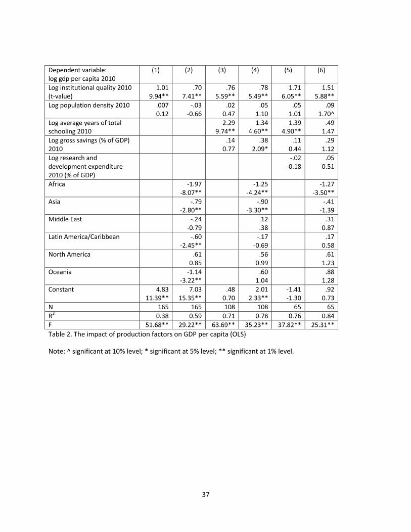
The Ordinary Least Squares (OLS) regressions results based on equation (7) are given in
table 2. Institutional quality and education are important factors of GDP per capita. Log saving
rates becomes significant when regional dummies are controlled (column 4). When research and
development are controlled for productivity, limited observations (65 observations) seem to be
problematic (column 5 and 6): the impacts of institutional quality are larger than other
specifications and the impact of education is not significant.
Next, I address the endogeniety and measurement error problems using cadastral survey
and triangulation dummies as instruments for estimating the degree of institutional quality. Table
4 provides the first stage regression results based on equation (9). This specification assumes that
institutional quality affects all other factors production and country specific parameters are
common across countries. Regression results suggest that triangulation is an important factor of
institutional quality, but cadastral survey is much more decisive factor of institutional quality.
The second stage regression results are provided in table 5. It shows that after controlling
endogeneity issues, the impact of institutional quality becomes larger (from 0.70 – 1.01 (table 2
column 1 and 2) to 2.08 – 2.33 (table 4 column 1 – 4)). Moreover, regional dummies which are
significant in OLS regression are not significant anymore, suggesting they are not necessary
when other variables are controlled.
However, education and saving rates can be endogenous, too. In order to address
endogeneity, table 5A uses the lagged values of education in 1950 and the lagged value of saving

21
rates in 1996. The first stage results suggest that when I control the lagged values of education
and gross savings, regional dummies become unnecessary instrumental variables (Sargan
statistics reject over-identification tests where a null hypothesis is instruments are healthy).
Without regional dummies, the instruments are healthy.
Table 6 column 1 and 2 provide the second stage regression results when education and
saving rates are considered as endogenous. The impact of institutional quality in 2SLS regression
(1.49 – 2.12) becomes larger than that of OLS (0.76 – 0.78, table 2 column 3 and 4). However,
the insignificant impact of education in column 2 also suggests that regional dummies are
unnecessary instruments when lagged variables of education and saving rates are controlled.
Table 5B provides regression results based on equation (10). This specification assumes
that baseline characteristics of countries are not common after controlling institutional qualities.
To control baseline differences of countries, it employs lagged values of education and grossing
saving rates as included instrumental variables. In other words, (productivity),
(saving rates) are assumed to be different thus controlled by lagged
values (however, (institutional quality) is assumed to be common. This impact is measured by
a constant). The 2nd
stage regression results in table 6 column 3 and 4 suggest that regression
results are robust.
Furthermore, population density can be endogenous. Table 4B column (5)A and (5)B
provide the first stage regression results using lagged value of population density as an
instruments. The 2nd
stage regression results in Table 6 column 5 suggest that regression results
are robust with endogenous population density.
Finally, the regression results are robust without European countries where mapping
techniques are originally invented (table 7).

22
7. Conclusion
The history of mapping provides an excellent opportunity for studying institutional
foundations of economic growth. European countries established triangulation networks and
developed them into civilian and cadastral mapping. However, in some developing countries
civilian use of mapping is still restricted due to military secrecy in mapping. The development
process of mapping allows to identify the mechanism linking mapping and institutional
foundations to economic growth. Instrumental variable estimates suggest that good mapping
stimulated economic growth.
Historical analysis suggests that good mapping facilitates a public finance problem by
solving boundary disputes and measuring plot size accurately. Moreover, this solution to a public
finance problem spilled over to private finance. A proper land survey defines boundaries enables
banks to accept land as collateral. Because land is the most abundant asset in agricultural
economies, its collateralization can provide a major boost for financial markets that nurture
economic development. In Asia, a secure land tenure system combined with financial market
developments encouraged investment, promoted new technology such as irrigation systems, and
consequently increased agricultural productivity.
The identified pathways suggest that good mapping could be a major stimulus to
economic development. Although good mapping can be the result of economic development, the
reverse causality problem is less severe in mapping when triangulation is employed. Surveying
errors are minimized if a chain of triangles at the largest scale is established first. Thus, the
accuracy of mapping in urban area depends on primary and secondary networks in rural areas.
Spatial information is critical for all economic activities. The survey of land made the
economy more manageable.

23
Appendix. Difficulties in mapping
Mapping requires a lot of technical foundations including datum, baseline, triangulation,
scale factors, and ellipsoid. European countries improved the accuracy of those foundational
values over time because a small error propagates to all mapping procedures. However, in many
developing countries those foundational values are not very accurate.
First, datums in developing countries may not be accurate. During the 20th century,
accuracies were commonly only good to a few hundred meters. Dr. Muneendra Kumar4, said that
there is no such thing as the “Indian Datum.” There is only a series of piecemeal regional
“adjustments” of field observations and there has never (ever!) been a unified classical datum
adjustment. However, other countries still refer the Indian Datum. For example, in 1954, the
triangulation of Thailand was adjusted to Indian 1916 datum based on 10 stations on the Burma
border. In 1960, the triangulation of Cambodia and Vietnam was adjusted holding fixed two
Cambodian stations connected to the Thailand adjustment of stations from the Cambodian-
Vietnam adjustment. North Vietnam was also adjusted to this system but with lower standards.
(Mugnier, Apr. 2007)
Second, scale factors and ellipsoids were not properly adjusted for developing countries.
The shape of Earth is not a perfect circle, thus the projection is based on an assumed ellipsoid.
For example, in Djibouti, the Italian observations of the geodetic distance from Gaabla-
Humarrasuh (1933-1934) was 13,060.72 m, but the French observations of the geodetic distance
(1934-1935) was 13,060.53 m. These differences were attributed to differences in the ellipsoids
adopted (Mugnier, Oct. 2008). Indeed, from 1950-1970 U.S. Army Topographic Engineer
4 retired Chief Geodesist of the United States National Geo-spatial Intelligence Agency.

24
Officers were issued a set of geodetic tables that in total weighted about 40 pounds and the set
was comprised of ellipsoidal geodetic functions for all five of the standard ellipsoids.
Thirdly, some countries still do not have accurate baselines. The geodetic survey of the
30th
Meridian East of Greenwich became a symbol of the progress of documenting the British
Empire borders in Africa. The Arc of the 30th
meridian was proposed as the foundation of
triangulation in the East African colonies. Observations on a portion of the arc in western
Uganda had been taken prior to 1914, and the triangulation net in Uganda was tied to it.
Surveying on the arc had been done in northern Rhodesia, and it was felt that it was important to
close the gap in the arc in Tanganyika. Martin Hotine surveyed the arc of the 30th
meridian in
Tanganyika between 4½° and 9° South during the years 1931-1933. Depletion of funds in late
1933 left a gap in the arc between 1½° and 4½° South. From July 1936 to August 1937, a survey
was conducted wholly within Tanganyika to fill the gap, consisting of observation angles and
some azimuths (Mugnier, Sep. 1999). However, the British survey was not completed in Africa.
Moreover, before the introduction of GPS system, land surveyors were in shortage. Thus,
building a local surveyor school and training surveyors were usually required. Without the
school and the trained surveyor, the land survey could not be completed as planned.
Finally, during the 19th
century, projection table computations were performed by hand
and all formulae were commonly truncated past the cubic term to ignore infinite series terms
considered at the time, too small to warrant the extra effort. For instance, the Lambert Conformal
Conic projection was used only to the cubic term in the formulae. This resulted in French Army
projection tables that have become part of the arcane lore of computational cartography. For
example, standard Lambert formulae will not work for Morocco and Algeria under certain
conditions, and the improper use of the fully conformal projection will yield computational

25
errors that can exceed 15 meters (Mugnier, Jun. 1999; Oct 2001), which is very critical in urban
areas and can generate boundary disputes in rural areas. However, some developing countries
still relies on old hand calculated computations.
References
Acemoglu, D. and S. Johnson. 2007. Disease and Development: The Effect of Life Expectancy
on Economic Growth. Journal of Political Economy. 115 (6): 925 – 985.
Acemoglu, D., S. Johnson, and J. Robinsion. 2002. Reversal of Fortune: Geography and
Institutions in the Making of the Modern World Income Distribution. The Quarterly
Journal of Economics. 117 (4): 1231-1294.
Dale, P. F. 1976. Cadastral Surveys within the Commonwealth. London: Her Majesty’s
Stationery Office.
De Soto, H. 2003. The Mystery of Capital: Why Capitalism Triumphs in the West and Fails
Everywhere Else. New York: Basic Books.
Kim, Seong-Hak. 2008. Ume Kenjiro and the Making of Korean Civil Law, 1906-1910. The
Journal of Japanese Studies 34 (1): 1-31.
Mugnier, Clifford J. 1997 – 2014. Grids and Datums. Photogrammetric Engineering & Remote
Sensing.
Rhee, Younghoon, Siwon Jang, Hiroshi Miyajima, and Takenori Matumoto. 1992. Hankuk
Guendae Suri Johap Yongu. SeoulL Iljogak.
Slabblers, P. J. 1990. Western and Indigenous Principles of Irrigation Water Distribution. In
Design for Sustainable Farmer Managed Irrigation Scheme in Sub-Saharan Africa.
Yoo, D. and R. H. Steckel. 2010. Property Rights and Financial Development: The Legacy of
Japanese Colonial Institutions. NBER Working Paper Series No. 16551.
26
Figure 1. A Contour Map and a military topographic map

27
Figure 2. A cadastral map
28
; thus,
.
Figure 3. Triangulation
d
c
α β

29
Figure 4. Triangulation networks

30
Figure 5. Resection

31
Figure 6. Triangulation Primary Stations
32
Figure 7. Secondary Stations inside Primary Stations
33
Figure 8. Horizontal and Natural Slope Distances
Figure 9. Distance measured at an altitude above sea level

34
Figure 10. Traditional Cadastral Map and Google Earth

35
Figure 11. 30th Meridian East of Greenwich

36
Mean Standard deviation
Min Max N
Log GDP per capita 2010 8.58 1.52 5.35 11.53 165
Log rule of law (percentile) 2010 3.64 .93 -.74 4.60 165
Log population density 2010 4.27 1.52 .54 9.93 165
Cadastral survey .28 .45 0 1 165
Triangulation before World War I .43 .49 0 1 165
Triangulation between World War I and World War II
.26 .44 0 1
165
Triangulation after World War II .23 .42 0 1 165
Existence of Triangulation .71 .45 0 1 165
Log average years of total schooling 2010
2.04 .41 .63 2.58 128
Log gross savings (% of GDP) 2010 2.94 .54 .40 4.09 125
Log research and development expenditure 2010 (% of GDP)
-.36 1.10 -3.13 1.37 72
Log population density 1950 3.12 1.71 -.69 8.93 165
Log average years of total schooling 1950
.69 1.03 -3.91 2.22 128
Log gross savings (% of GDP) 1996 2.81 .64 -.01 4.34 130
Log research and development expenditure 1996 (% of GDP)
-.48 1.11 -4.41 1.01 50
Table 1. Descriptive Statistics (165 countries)
37
Dependent variable: log gdp per capita 2010
(1) (2) (3) (4) (5) (6)
Log institutional quality 2010 (t-value)
1.01 9.94**
.70 7.41**
.76 5.59**
.78 5.49**
1.71 6.05**
1.51 5.88**
Log population density 2010 .007 0.12
-.03 -0.66
.02 0.47
.05 1.10
.05 1.01
.09 1.70^
Log average years of total schooling 2010
2.29 9.74**
1.34 4.60**
1.39 4.90**
.49 1.47
Log gross savings (% of GDP) 2010
.14 0.77
.38 2.09*
.11 0.44
.29 1.12
Log research and development expenditure 2010 (% of GDP)
-.02 -0.18
.05 0.51
Africa -1.97 -8.07**
-1.25 -4.24**
-1.27 -3.50**
Asia -.79 -2.80**
-.90 -3.30**
-.41 -1.39
Middle East -.24 -0.79
.12 .38
.31 0.87
Latin America/Caribbean -.60 -2.45**
-.17 -0.69
.17 0.58
North America .61 0.85
.56 0.99
.61 1.23
Oceania -1.14 -3.22**
.60 1.04
.88 1.28
Constant 4.83 11.39**
7.03 15.35**
.48 0.70
2.01 2.33**
-1.41 -1.30
.92 0.73
N 165 165 108 108 65 65
R2 0.38 0.59 0.71 0.78 0.76 0.84
F 51.68** 29.22** 63.69** 35.23** 37.82** 25.31**
Table 2. The impact of production factors on GDP per capita (OLS)
Note: ^ significant at 10% level; * significant at 5% level; ** significant at 1% level.

38
Dependent variable: log institutional quality 2010
(1) (2) (3) (4)
Triangulation (t-value)
.27 1.74^
.10 0.67
.11 0.78
Cadastral .70 4.21**
.67 4.01**
.47 2.87**
Geodetic survey 1914-1945 -.29 -1.73^
-.12 -0.74
-.13 -0.78
-.11 -0.65
Geodetic survey after 1945 -.22 -1.25
-.04 -0.25
-.03 -0.18
-.04 -0.26
Log population density 2010 .11 2.39*
.07 1.68^
.07 1.68^
.08 1.96*
Africa -.77 -3.86**
Asia -.78 -3.50**
Middle East -.13 -0.51
Latin America / Caribbean -.33 -1.47
North America .25 0.42
Oceania .003 0.01
Constant 3.10 11.68**
3.16 14.32**
3.09 12.19**
3.49 12.76**
N 165 165 165 165
R2 0.0847 0.1661 0.1688 0.2953
Partial R2 0.0465 0.1313 0.1341 0.0737
F 2.59 7.97 6.15 3.04
Over-identification test .19 (p = 0.9080)
.68 (p = 0.7105)
.31 (p = 0.9574)
.45 (p = 0.9285)
Table 3. The impact of mapping on institutional quality (2SLS/1st stage)
Note: ^ significant at 10% level; * significant at 5% level; ** significant at 1% level.

39
Dependent variable: log gdp per capita 2010
(1) (2) (3) (4)
Log institutional quality 2010 (t-value)
2.08 3.43**
2.33 5.86**
2.28 5.91**
2.33 4.04**
Log population density 2010 -.12 -1.13
-.15 -1.54
-.14 -1.52
-.22 -2.04*
Africa -.31 -0.45
Asia .72 1.04
Middle East .32 0.61
Latin America/Caribbean .44 0.82
North America -.27 -0.22
Oceania -.83 -1.39
Constant 1.50 0.78
.73 0.56
.86 0.68
.95 0.43
N 165 165 165 165
Table 4. The impact of institutional quality on GDP per capita (2SLS/2nd stage)
Note: ^ significant at 10% level; * significant at 5% level; ** significant at 1% level.

40
Dependent variable: log institutional quality
2010
Dependent variable: log average years of total schooling 2010
Dependent variable: Log gross savings 2010
Cadastral survey
(t-value) .29
2.17* .18
1.42 -.01
-0.30 .01
0.31 .02
0.19 .05
0.49
Geodetic survey 1914-1945
-.32 -2.24*
-.11 -0.78
-.07 -1.39
-.07 -1.25
-.03 -0.32
.03 0.26
Geodetic survey after 1945
-.26 -1.68^
-.07 -0.46
-.15 -2.65**
-.15 -2.49*
.04 0.35
.08 0.70
Log population density 2010
.01 0.26
.01 0.30
.01 1.25
.007 0.53
.02 0.81
-.008 -0.26
Log average years of total schooling 1950
.21 2.98**
.33 3.23**
.32 12.26**
.25 6.39**
-.04 -0.73
-.007 -0.09
Log gross savings (% of GDP) 1996
.07 0.68
.08 0.78
.15 4.11**
.14 3.52**
.35 4.25**
.23 2.78**
Africa .12 0.58
-.20 -2.38**
-.07 -0.41
Asia -.21 -1.16
-.04 -0.60
.47 3.12**
Middle East .29 1.26
.01 0.17
.14 0.77
Latin America / Caribbean
-.58 -3.35**
-.04 -0.59
-.06 -0.50
North America .01 0.04
.01 0.09
-.10 -0.33
Oceania .07 0.20
-.07 -0.52
.007 0.02
Constant 3.46 10.41**
3.38 9.43**
1.34 11.17**
1.52 10.87**
1.85 7.12**
2.21 7.62**
N 100 100 100 100 100 100
R2 0.3756 0.5138 0.7909 0.8087 0.1966 0.3319
Partial R2 0.1005 0.0295 0.2077 0.0627 0.1525 0.0752
F 9.32** 7.66** 58.61** 30.65** 3.79** 3.60**
Over-identification test 2.28 (p=0.31)
6.00* (p =0.04)
2.28 (p=0.31)
6.00* (p =0.04)
2.28 (p=0.31)
6.00* (p =0.04)
Table 5A. 1st stage results (table 6, (1) – (2)), endogenous education and saving rates
Note: ^ significant at 10% level; * significant at 5% level; ** significant at 1% level.

41
(3) Dep var: log institutional quality 2010
(4) Dep var: log institutional quality 2010
(5)A Dep var: log institutional quality 2010
(5)B
Dep var: log population density 2010
Cadastral survey
(t-value) .32
2.57* .06
0.52 .32
2.53* -.03
-0.31 Geodetic survey 1914-1945 -.34
-2.59* -.26
-1.65 -.33
-2.45* .35
3.12** Geodetic survey after 1945 -.23
-1.54 -.58
-3.64** -.22
-1.47 .37
2.93 Log population density 2010 .01
0.44 -.005 -0.13
Log population density 1950 .02 0.73
.92 32.47**
Log average years of total schooling 1950
.21 3.75**
.05 0.59
.21 3.66**
-.26 -5.37**
Log gross savings (% of GDP) 1996
.07 0.73
.15 0.91
.07 0.77
.13 1.65
Log research and development expenditure 1996 (% of GDP)
.21 3.33**
Constant 3.40 10.81**
3.75 7.77**
3.38 11.22**
.99 3.91
N 109 42 109 109 R
2 0.4135 0.6798 0.4154 0.9146
Partial R2 0.1558 0.3093 0.1518 0.8284
F 11.98** 10.31** 12.08** 182.17** Over-identification test 2.12
(p = 0.34) .63
(p = 0.72) 2.09
(p = 0.35) 2.09
(p = 0.35)
Table 5B. 1st stage results (table 6, (3) – (5)), using lagged variables to control baseline differences
Note: ^ significant at 10% level; * significant at 5% level; ** significant at 1% level.

42
Dependent variable: log gdp per capita 2010
(1)
(2)
(3) (4) (5)
Log institutional quality 2010 (t-value)
1.49 2.93**
2.12 1.69^
1.82 3.97**
1.43 3.03**
1.83 3.92**
Log population density 2010 -.05 -0.79
-.005 -0.06
-.04 -0.66
-.08 -1.17
-.05 -0.71
Log average years of total schooling 2010
1.82 3.14**
-.03 -0.02
Log gross savings (% of GDP) 2010
.34 0.63
1.34 1.33
Log average years of total schooling 1950
.53 2.72**
.50 2.96**
.30 1.64^
Log gross savings (% of GDP) 1996
.31 1.69^
.47 1.61
.53 2.70**
Log research and development expenditure 1996 (% of GDP)
.09 0.51
Africa -1.33 -1.88^
Asia -1.15 -1.46
Middle East -.23 -0.38
Latin America/Caribbean .74 0.95
North America .38 0.46
Oceania .08 0.10
Constant -2.98 -0.98
.15 0.10
1.95 1.07
.14 0.10
N 100 100 109 42 109
Over-identification test (1st stage)
2.28 (p=0.31)
6.00* (p=0.04)
2.12 (p=0.34)
.63 (p=0.72)
2.09 (p=0.35)
Table 6. The impact of institutional quality, education, and saving rates on GDP per capita (2SLS/ 2nd
stage)
Note: ^ significant at 10% level; * significant at 5% level; ** significant at 1% level.

43
Dependent variable: log gdp per capita 2010
(1) OLS
(2) 2SLS
(3) 2SLS
(4) 2SLS
(5) 2SLS
Log institutional quality 2010 (t-value)
.50 3.90**
1.78 3.74**
(Instrumented)
1.42 2.71**
(instrumented)
.96 1.45
(Instrumented)
1.49 2.44**
(Instrumented) Log population density 2010 .02
0.37 .00
1.20 .00
0.07 -.08
-1.17 -.04
-0.53
Log average years of total schooling 2010
2.06 8.21**
1.69 3.73**
2.32 3.60**
(Instrumented)
Log gross savings (% of GDP) 2010 .20 1.73^
.26 1.05
-.07 -0.13
(Instrumented)
Log average years of total schooling 1950
.37 1.92^
Log gross savings (% of GDP) 1996 .54 2.50**
Constant 1.62 2.56*
1.98 1.20
-1.11 -0.75
.48 0.25
1.25 0.65
N 88 130 77 70 79
Over-identification test (1st stage)
.75 (p = 0.68)
1.26 (p = 0.53)
1.58 (p = 0.45)
1.41 (p = 0.49)
Partial R2, the first stage 0.0859 0.1105 0.0617 (institution)
0.1886 (education)
0.1752 (savings)
0.1061
Table 7. The impact of institutional quality, education, and saving rates on GDP per capita (2SLS/ 2nd
stage, without European countries)
Note: ^ significant at 10% level; * significant at 5% level; ** significant at 1% level.


