Download - Mathematics Grade 10 PDF

FHSST Authors
The Free High School Science Texts:Textbooks for High School StudentsStudying the SciencesMathematicsGrades 10 - 12
Version 0September 17, 2008

ii

iii
Copyright 2007 “Free High School Science Texts”Permission is granted to copy, distribute and/or modify this document under theterms of the GNU Free Documentation License, Version 1.2 or any later versionpublished by the Free Software Foundation; with no Invariant Sections, no Front-Cover Texts, and no Back-Cover Texts. A copy of the license is included in thesection entitled “GNU Free Documentation License”.
STOP!!!!
Did you notice the FREEDOMS we’ve granted you?
Our copyright license is different! It grants freedoms
rather than just imposing restrictions like all those other
textbooks you probably own or use.
• We know people copy textbooks illegally but we would LOVE it if you copied
our’s - go ahead copy to your hearts content, legally!
• Publishers revenue is generated by controlling the market, we don’t want any
money, go ahead, distribute our books far and wide - we DARE you!
• Ever wanted to change your textbook? Of course you have! Go ahead change
ours, make your own version, get your friends together, rip it apart and put
it back together the way you like it. That’s what we really want!
• Copy, modify, adapt, enhance, share, critique, adore, and contextualise. Do it
all, do it with your colleagues, your friends or alone but get involved! Together
we can overcome the challenges our complex and diverse country presents.
• So what is the catch? The only thing you can’t do is take this book, make
a few changes and then tell others that they can’t do the same with your
changes. It’s share and share-alike and we know you’ll agree that is only fair.
• These books were written by volunteers who want to help support education,
who want the facts to be freely available for teachers to copy, adapt and
re-use. Thousands of hours went into making them and they are a gift to
everyone in the education community.

iv

FHSST Core Team
Mark Horner ; Samuel Halliday ; Sarah Blyth ; Rory Adams ; Spencer Wheaton
FHSST Editors
Jaynie Padayachee ; Joanne Boulle ; Diana Mulcahy ; Annette Nell ; Rene Toerien ; Donovan
Whitfield
FHSST Contributors
Rory Adams ; Prashant Arora ; Richard Baxter ; Dr. Sarah Blyth ; Sebastian Bodenstein ;
Graeme Broster ; Richard Case ; Brett Cocks ; Tim Crombie ; Dr. Anne Dabrowski ; Laura
Daniels ; Sean Dobbs ; Fernando Durrell ; Dr. Dan Dwyer ; Frans van Eeden ; Giovanni
Franzoni ; Ingrid von Glehn ; Tamara von Glehn ; Lindsay Glesener ; Dr. Vanessa Godfrey ; Dr.
Johan Gonzalez ; Hemant Gopal ; Umeshree Govender ; Heather Gray ; Lynn Greeff ; Dr. Tom
Gutierrez ; Brooke Haag ; Kate Hadley ; Dr. Sam Halliday ; Asheena Hanuman ; Neil Hart ;
Nicholas Hatcher ; Dr. Mark Horner ; Mfandaidza Hove ; Robert Hovden ; Jennifer Hsieh ;
Clare Johnson ; Luke Jordan ; Tana Joseph ; Dr. Jennifer Klay ; Lara Kruger ; Sihle Kubheka ;
Andrew Kubik ; Dr. Marco van Leeuwen ; Dr. Anton Machacek ; Dr. Komal Maheshwari ;
Kosma von Maltitz ; Nicole Masureik ; John Mathew ; JoEllen McBride ; Nikolai Meures ;
Riana Meyer ; Jenny Miller ; Abdul Mirza ; Asogan Moodaly ; Jothi Moodley ; Nolene Naidu ;
Tyrone Negus ; Thomas O’Donnell ; Dr. Markus Oldenburg ; Dr. Jaynie Padayachee ;
Nicolette Pekeur ; Sirika Pillay ; Jacques Plaut ; Andrea Prinsloo ; Joseph Raimondo ; Sanya
Rajani ; Prof. Sergey Rakityansky ; Alastair Ramlakan ; Razvan Remsing ; Max Richter ; Sean
Riddle ; Evan Robinson ; Dr. Andrew Rose ; Bianca Ruddy ; Katie Russell ; Duncan Scott ;
Helen Seals ; Ian Sherratt ; Roger Sieloff ; Bradley Smith ; Greg Solomon ; Mike Stringer ;
Shen Tian ; Robert Torregrosa ; Jimmy Tseng ; Helen Waugh ; Dr. Dawn Webber ; Michelle
Wen ; Dr. Alexander Wetzler ; Dr. Spencer Wheaton ; Vivian White ; Dr. Gerald Wigger ;
Harry Wiggins ; Wendy Williams ; Julie Wilson ; Andrew Wood ; Emma Wormauld ; Sahal
Yacoob ; Jean Youssef
Contributors and editors have made a sincere effort to produce an accurate and useful resource.Should you have suggestions, find mistakes or be prepared to donate material for inclusion,please don’t hesitate to contact us. We intend to work with all who are willing to help make
this a continuously evolving resource!
www.fhsst.org
v

vi

Contents
I Basics 1
1 Introduction to Book 3
1.1 The Language of Mathematics . . . . . . . . . . . . . . . . . . . . . . . . . . . 3
II Grade 10 5
2 Review of Past Work 7
2.1 Introduction . . . . . . . . . . . . . . . . . . . . . . . . . . . . . . . . . . . . . 7
2.2 What is a number? . . . . . . . . . . . . . . . . . . . . . . . . . . . . . . . . . 7
2.3 Sets . . . . . . . . . . . . . . . . . . . . . . . . . . . . . . . . . . . . . . . . . 7
2.4 Letters and Arithmetic . . . . . . . . . . . . . . . . . . . . . . . . . . . . . . . 8
2.5 Addition and Subtraction . . . . . . . . . . . . . . . . . . . . . . . . . . . . . . 9
2.6 Multiplication and Division . . . . . . . . . . . . . . . . . . . . . . . . . . . . . 9
2.7 Brackets . . . . . . . . . . . . . . . . . . . . . . . . . . . . . . . . . . . . . . . 9
2.8 Negative Numbers . . . . . . . . . . . . . . . . . . . . . . . . . . . . . . . . . . 10
2.8.1 What is a negative number? . . . . . . . . . . . . . . . . . . . . . . . . 10
2.8.2 Working with Negative Numbers . . . . . . . . . . . . . . . . . . . . . . 11
2.8.3 Living Without the Number Line . . . . . . . . . . . . . . . . . . . . . . 12
2.9 Rearranging Equations . . . . . . . . . . . . . . . . . . . . . . . . . . . . . . . 13
2.10 Fractions and Decimal Numbers . . . . . . . . . . . . . . . . . . . . . . . . . . 15
2.11 Scientific Notation . . . . . . . . . . . . . . . . . . . . . . . . . . . . . . . . . . 16
2.12 Real Numbers . . . . . . . . . . . . . . . . . . . . . . . . . . . . . . . . . . . . 16
2.12.1 Natural Numbers . . . . . . . . . . . . . . . . . . . . . . . . . . . . . . 17
2.12.2 Integers . . . . . . . . . . . . . . . . . . . . . . . . . . . . . . . . . . . 17
2.12.3 Rational Numbers . . . . . . . . . . . . . . . . . . . . . . . . . . . . . . 17
2.12.4 Irrational Numbers . . . . . . . . . . . . . . . . . . . . . . . . . . . . . 19
2.13 Mathematical Symbols . . . . . . . . . . . . . . . . . . . . . . . . . . . . . . . 20
2.14 Infinity . . . . . . . . . . . . . . . . . . . . . . . . . . . . . . . . . . . . . . . . 20
2.15 End of Chapter Exercises . . . . . . . . . . . . . . . . . . . . . . . . . . . . . . 21
3 Rational Numbers - Grade 10 23
3.1 Introduction . . . . . . . . . . . . . . . . . . . . . . . . . . . . . . . . . . . . . 23
3.2 The Big Picture of Numbers . . . . . . . . . . . . . . . . . . . . . . . . . . . . 23
3.3 Definition . . . . . . . . . . . . . . . . . . . . . . . . . . . . . . . . . . . . . . 23
vii

CONTENTS CONTENTS
3.4 Forms of Rational Numbers . . . . . . . . . . . . . . . . . . . . . . . . . . . . . 24
3.5 Converting Terminating Decimals into Rational Numbers . . . . . . . . . . . . . 25
3.6 Converting Repeating Decimals into Rational Numbers . . . . . . . . . . . . . . 25
3.7 Summary . . . . . . . . . . . . . . . . . . . . . . . . . . . . . . . . . . . . . . . 26
3.8 End of Chapter Exercises . . . . . . . . . . . . . . . . . . . . . . . . . . . . . . 27
4 Exponentials - Grade 10 29
4.1 Introduction . . . . . . . . . . . . . . . . . . . . . . . . . . . . . . . . . . . . . 29
4.2 Definition . . . . . . . . . . . . . . . . . . . . . . . . . . . . . . . . . . . . . . 29
4.3 Laws of Exponents . . . . . . . . . . . . . . . . . . . . . . . . . . . . . . . . . . 30
4.3.1 Exponential Law 1: a0 = 1 . . . . . . . . . . . . . . . . . . . . . . . . . 30
4.3.2 Exponential Law 2: am × an = am+n . . . . . . . . . . . . . . . . . . . 30
4.3.3 Exponential Law 3: a−n = 1an , a 6= 0 . . . . . . . . . . . . . . . . . . . . 31
4.3.4 Exponential Law 4: am ÷ an = am−n . . . . . . . . . . . . . . . . . . . 32
4.3.5 Exponential Law 5: (ab)n = anbn . . . . . . . . . . . . . . . . . . . . . 32
4.3.6 Exponential Law 6: (am)n = amn . . . . . . . . . . . . . . . . . . . . . 33
4.4 End of Chapter Exercises . . . . . . . . . . . . . . . . . . . . . . . . . . . . . . 34
5 Estimating Surds - Grade 10 37
5.1 Introduction . . . . . . . . . . . . . . . . . . . . . . . . . . . . . . . . . . . . . 37
5.2 Drawing Surds on the Number Line (Optional) . . . . . . . . . . . . . . . . . . 38
5.3 End of Chapter Excercises . . . . . . . . . . . . . . . . . . . . . . . . . . . . . . 39
6 Irrational Numbers and Rounding Off - Grade 10 41
6.1 Introduction . . . . . . . . . . . . . . . . . . . . . . . . . . . . . . . . . . . . . 41
6.2 Irrational Numbers . . . . . . . . . . . . . . . . . . . . . . . . . . . . . . . . . . 41
6.3 Rounding Off . . . . . . . . . . . . . . . . . . . . . . . . . . . . . . . . . . . . 42
6.4 End of Chapter Exercises . . . . . . . . . . . . . . . . . . . . . . . . . . . . . . 43
7 Number Patterns - Grade 10 45
7.1 Common Number Patterns . . . . . . . . . . . . . . . . . . . . . . . . . . . . . 45
7.1.1 Special Sequences . . . . . . . . . . . . . . . . . . . . . . . . . . . . . . 46
7.2 Make your own Number Patterns . . . . . . . . . . . . . . . . . . . . . . . . . . 46
7.3 Notation . . . . . . . . . . . . . . . . . . . . . . . . . . . . . . . . . . . . . . . 47
7.3.1 Patterns and Conjecture . . . . . . . . . . . . . . . . . . . . . . . . . . 49
7.4 Exercises . . . . . . . . . . . . . . . . . . . . . . . . . . . . . . . . . . . . . . . 50
8 Finance - Grade 10 53
8.1 Introduction . . . . . . . . . . . . . . . . . . . . . . . . . . . . . . . . . . . . . 53
8.2 Foreign Exchange Rates . . . . . . . . . . . . . . . . . . . . . . . . . . . . . . . 53
8.2.1 How much is R1 really worth? . . . . . . . . . . . . . . . . . . . . . . . 53
8.2.2 Cross Currency Exchange Rates . . . . . . . . . . . . . . . . . . . . . . 56
8.2.3 Enrichment: Fluctuating exchange rates . . . . . . . . . . . . . . . . . . 57
8.3 Being Interested in Interest . . . . . . . . . . . . . . . . . . . . . . . . . . . . . 58
viii

CONTENTS CONTENTS
8.4 Simple Interest . . . . . . . . . . . . . . . . . . . . . . . . . . . . . . . . . . . . 59
8.4.1 Other Applications of the Simple Interest Formula . . . . . . . . . . . . . 61
8.5 Compound Interest . . . . . . . . . . . . . . . . . . . . . . . . . . . . . . . . . 63
8.5.1 Fractions add up to the Whole . . . . . . . . . . . . . . . . . . . . . . . 65
8.5.2 The Power of Compound Interest . . . . . . . . . . . . . . . . . . . . . . 65
8.5.3 Other Applications of Compound Growth . . . . . . . . . . . . . . . . . 67
8.6 Summary . . . . . . . . . . . . . . . . . . . . . . . . . . . . . . . . . . . . . . . 68
8.6.1 Definitions . . . . . . . . . . . . . . . . . . . . . . . . . . . . . . . . . . 68
8.6.2 Equations . . . . . . . . . . . . . . . . . . . . . . . . . . . . . . . . . . 68
8.7 End of Chapter Exercises . . . . . . . . . . . . . . . . . . . . . . . . . . . . . . 69
9 Products and Factors - Grade 10 71
9.1 Introduction . . . . . . . . . . . . . . . . . . . . . . . . . . . . . . . . . . . . . 71
9.2 Recap of Earlier Work . . . . . . . . . . . . . . . . . . . . . . . . . . . . . . . . 71
9.2.1 Parts of an Expression . . . . . . . . . . . . . . . . . . . . . . . . . . . . 71
9.2.2 Product of Two Binomials . . . . . . . . . . . . . . . . . . . . . . . . . 71
9.2.3 Factorisation . . . . . . . . . . . . . . . . . . . . . . . . . . . . . . . . . 72
9.3 More Products . . . . . . . . . . . . . . . . . . . . . . . . . . . . . . . . . . . . 74
9.4 Factorising a Quadratic . . . . . . . . . . . . . . . . . . . . . . . . . . . . . . . 76
9.5 Factorisation by Grouping . . . . . . . . . . . . . . . . . . . . . . . . . . . . . . 79
9.6 Simplification of Fractions . . . . . . . . . . . . . . . . . . . . . . . . . . . . . . 80
9.7 End of Chapter Exercises . . . . . . . . . . . . . . . . . . . . . . . . . . . . . . 82
10 Equations and Inequalities - Grade 10 83
10.1 Strategy for Solving Equations . . . . . . . . . . . . . . . . . . . . . . . . . . . 83
10.2 Solving Linear Equations . . . . . . . . . . . . . . . . . . . . . . . . . . . . . . 84
10.3 Solving Quadratic Equations . . . . . . . . . . . . . . . . . . . . . . . . . . . . 89
10.4 Exponential Equations of the form ka(x+p) = m . . . . . . . . . . . . . . . . . . 93
10.4.1 Algebraic Solution . . . . . . . . . . . . . . . . . . . . . . . . . . . . . . 93
10.5 Linear Inequalities . . . . . . . . . . . . . . . . . . . . . . . . . . . . . . . . . . 96
10.6 Linear Simultaneous Equations . . . . . . . . . . . . . . . . . . . . . . . . . . . 99
10.6.1 Finding solutions . . . . . . . . . . . . . . . . . . . . . . . . . . . . . . 99
10.6.2 Graphical Solution . . . . . . . . . . . . . . . . . . . . . . . . . . . . . . 99
10.6.3 Solution by Substitution . . . . . . . . . . . . . . . . . . . . . . . . . . 101
10.7 Mathematical Models . . . . . . . . . . . . . . . . . . . . . . . . . . . . . . . . 103
10.7.1 Introduction . . . . . . . . . . . . . . . . . . . . . . . . . . . . . . . . . 103
10.7.2 Problem Solving Strategy . . . . . . . . . . . . . . . . . . . . . . . . . . 104
10.7.3 Application of Mathematical Modelling . . . . . . . . . . . . . . . . . . 104
10.7.4 End of Chapter Exercises . . . . . . . . . . . . . . . . . . . . . . . . . . 106
10.8 Introduction to Functions and Graphs . . . . . . . . . . . . . . . . . . . . . . . 107
10.9 Functions and Graphs in the Real-World . . . . . . . . . . . . . . . . . . . . . . 107
10.10Recap . . . . . . . . . . . . . . . . . . . . . . . . . . . . . . . . . . . . . . . . 107
ix

CONTENTS CONTENTS
10.10.1Variables and Constants . . . . . . . . . . . . . . . . . . . . . . . . . . . 107
10.10.2Relations and Functions . . . . . . . . . . . . . . . . . . . . . . . . . . . 108
10.10.3The Cartesian Plane . . . . . . . . . . . . . . . . . . . . . . . . . . . . . 108
10.10.4Drawing Graphs . . . . . . . . . . . . . . . . . . . . . . . . . . . . . . . 109
10.10.5Notation used for Functions . . . . . . . . . . . . . . . . . . . . . . . . 110
10.11Characteristics of Functions - All Grades . . . . . . . . . . . . . . . . . . . . . . 112
10.11.1Dependent and Independent Variables . . . . . . . . . . . . . . . . . . . 112
10.11.2Domain and Range . . . . . . . . . . . . . . . . . . . . . . . . . . . . . 113
10.11.3 Intercepts with the Axes . . . . . . . . . . . . . . . . . . . . . . . . . . 113
10.11.4Turning Points . . . . . . . . . . . . . . . . . . . . . . . . . . . . . . . . 114
10.11.5Asymptotes . . . . . . . . . . . . . . . . . . . . . . . . . . . . . . . . . 114
10.11.6Lines of Symmetry . . . . . . . . . . . . . . . . . . . . . . . . . . . . . 114
10.11.7 Intervals on which the Function Increases/Decreases . . . . . . . . . . . 114
10.11.8Discrete or Continuous Nature of the Graph . . . . . . . . . . . . . . . . 114
10.12Graphs of Functions . . . . . . . . . . . . . . . . . . . . . . . . . . . . . . . . . 116
10.12.1Functions of the form y = ax + q . . . . . . . . . . . . . . . . . . . . . 116
10.12.2Functions of the Form y = ax2 + q . . . . . . . . . . . . . . . . . . . . . 120
10.12.3Functions of the Form y = ax
+ q . . . . . . . . . . . . . . . . . . . . . . 125
10.12.4Functions of the Form y = ab(x) + q . . . . . . . . . . . . . . . . . . . . 129
10.13End of Chapter Exercises . . . . . . . . . . . . . . . . . . . . . . . . . . . . . . 133
11 Average Gradient - Grade 10 Extension 135
11.1 Introduction . . . . . . . . . . . . . . . . . . . . . . . . . . . . . . . . . . . . . 135
11.2 Straight-Line Functions . . . . . . . . . . . . . . . . . . . . . . . . . . . . . . . 135
11.3 Parabolic Functions . . . . . . . . . . . . . . . . . . . . . . . . . . . . . . . . . 136
11.4 End of Chapter Exercises . . . . . . . . . . . . . . . . . . . . . . . . . . . . . . 138
12 Geometry Basics 139
12.1 Introduction . . . . . . . . . . . . . . . . . . . . . . . . . . . . . . . . . . . . . 139
12.2 Points and Lines . . . . . . . . . . . . . . . . . . . . . . . . . . . . . . . . . . . 139
12.3 Angles . . . . . . . . . . . . . . . . . . . . . . . . . . . . . . . . . . . . . . . . 140
12.3.1 Measuring angles . . . . . . . . . . . . . . . . . . . . . . . . . . . . . . 141
12.3.2 Special Angles . . . . . . . . . . . . . . . . . . . . . . . . . . . . . . . . 141
12.3.3 Special Angle Pairs . . . . . . . . . . . . . . . . . . . . . . . . . . . . . 143
12.3.4 Parallel Lines intersected by Transversal Lines . . . . . . . . . . . . . . . 143
12.4 Polygons . . . . . . . . . . . . . . . . . . . . . . . . . . . . . . . . . . . . . . . 147
12.4.1 Triangles . . . . . . . . . . . . . . . . . . . . . . . . . . . . . . . . . . . 147
12.4.2 Quadrilaterals . . . . . . . . . . . . . . . . . . . . . . . . . . . . . . . . 152
12.4.3 Other polygons . . . . . . . . . . . . . . . . . . . . . . . . . . . . . . . 155
12.4.4 Extra . . . . . . . . . . . . . . . . . . . . . . . . . . . . . . . . . . . . . 156
12.5 Exercises . . . . . . . . . . . . . . . . . . . . . . . . . . . . . . . . . . . . . . . 157
12.5.1 Challenge Problem . . . . . . . . . . . . . . . . . . . . . . . . . . . . . 159
x

CONTENTS CONTENTS
13 Geometry - Grade 10 161
13.1 Introduction . . . . . . . . . . . . . . . . . . . . . . . . . . . . . . . . . . . . . 161
13.2 Right Prisms and Cylinders . . . . . . . . . . . . . . . . . . . . . . . . . . . . . 161
13.2.1 Surface Area . . . . . . . . . . . . . . . . . . . . . . . . . . . . . . . . . 162
13.2.2 Volume . . . . . . . . . . . . . . . . . . . . . . . . . . . . . . . . . . . 164
13.3 Polygons . . . . . . . . . . . . . . . . . . . . . . . . . . . . . . . . . . . . . . . 167
13.3.1 Similarity of Polygons . . . . . . . . . . . . . . . . . . . . . . . . . . . . 167
13.4 Co-ordinate Geometry . . . . . . . . . . . . . . . . . . . . . . . . . . . . . . . . 171
13.4.1 Introduction . . . . . . . . . . . . . . . . . . . . . . . . . . . . . . . . . 171
13.4.2 Distance between Two Points . . . . . . . . . . . . . . . . . . . . . . . . 172
13.4.3 Calculation of the Gradient of a Line . . . . . . . . . . . . . . . . . . . . 173
13.4.4 Midpoint of a Line . . . . . . . . . . . . . . . . . . . . . . . . . . . . . 174
13.5 Transformations . . . . . . . . . . . . . . . . . . . . . . . . . . . . . . . . . . . 177
13.5.1 Translation of a Point . . . . . . . . . . . . . . . . . . . . . . . . . . . . 177
13.5.2 Reflection of a Point . . . . . . . . . . . . . . . . . . . . . . . . . . . . 179
13.6 End of Chapter Exercises . . . . . . . . . . . . . . . . . . . . . . . . . . . . . . 185
14 Trigonometry - Grade 10 189
14.1 Introduction . . . . . . . . . . . . . . . . . . . . . . . . . . . . . . . . . . . . . 189
14.2 Where Trigonometry is Used . . . . . . . . . . . . . . . . . . . . . . . . . . . . 190
14.3 Similarity of Triangles . . . . . . . . . . . . . . . . . . . . . . . . . . . . . . . . 190
14.4 Definition of the Trigonometric Functions . . . . . . . . . . . . . . . . . . . . . 191
14.5 Simple Applications of Trigonometric Functions . . . . . . . . . . . . . . . . . . 195
14.5.1 Height and Depth . . . . . . . . . . . . . . . . . . . . . . . . . . . . . . 195
14.5.2 Maps and Plans . . . . . . . . . . . . . . . . . . . . . . . . . . . . . . . 197
14.6 Graphs of Trigonometric Functions . . . . . . . . . . . . . . . . . . . . . . . . . 199
14.6.1 Graph of sin θ . . . . . . . . . . . . . . . . . . . . . . . . . . . . . . . . 199
14.6.2 Functions of the form y = a sin(x) + q . . . . . . . . . . . . . . . . . . . 200
14.6.3 Graph of cos θ . . . . . . . . . . . . . . . . . . . . . . . . . . . . . . . . 202
14.6.4 Functions of the form y = a cos(x) + q . . . . . . . . . . . . . . . . . . 202
14.6.5 Comparison of Graphs of sin θ and cos θ . . . . . . . . . . . . . . . . . . 204
14.6.6 Graph of tan θ . . . . . . . . . . . . . . . . . . . . . . . . . . . . . . . . 204
14.6.7 Functions of the form y = a tan(x) + q . . . . . . . . . . . . . . . . . . 205
14.7 End of Chapter Exercises . . . . . . . . . . . . . . . . . . . . . . . . . . . . . . 208
15 Statistics - Grade 10 211
15.1 Introduction . . . . . . . . . . . . . . . . . . . . . . . . . . . . . . . . . . . . . 211
15.2 Recap of Earlier Work . . . . . . . . . . . . . . . . . . . . . . . . . . . . . . . . 211
15.2.1 Data and Data Collection . . . . . . . . . . . . . . . . . . . . . . . . . . 211
15.2.2 Methods of Data Collection . . . . . . . . . . . . . . . . . . . . . . . . . 212
15.2.3 Samples and Populations . . . . . . . . . . . . . . . . . . . . . . . . . . 213
15.3 Example Data Sets . . . . . . . . . . . . . . . . . . . . . . . . . . . . . . . . . 213
xi

CONTENTS CONTENTS
15.3.1 Data Set 1: Tossing a Coin . . . . . . . . . . . . . . . . . . . . . . . . . 213
15.3.2 Data Set 2: Casting a die . . . . . . . . . . . . . . . . . . . . . . . . . . 213
15.3.3 Data Set 3: Mass of a Loaf of Bread . . . . . . . . . . . . . . . . . . . . 214
15.3.4 Data Set 4: Global Temperature . . . . . . . . . . . . . . . . . . . . . . 214
15.3.5 Data Set 5: Price of Petrol . . . . . . . . . . . . . . . . . . . . . . . . . 215
15.4 Grouping Data . . . . . . . . . . . . . . . . . . . . . . . . . . . . . . . . . . . . 215
15.4.1 Exercises - Grouping Data . . . . . . . . . . . . . . . . . . . . . . . . . 216
15.5 Graphical Representation of Data . . . . . . . . . . . . . . . . . . . . . . . . . . 217
15.5.1 Bar and Compound Bar Graphs . . . . . . . . . . . . . . . . . . . . . . . 217
15.5.2 Histograms and Frequency Polygons . . . . . . . . . . . . . . . . . . . . 217
15.5.3 Pie Charts . . . . . . . . . . . . . . . . . . . . . . . . . . . . . . . . . . 219
15.5.4 Line and Broken Line Graphs . . . . . . . . . . . . . . . . . . . . . . . . 220
15.5.5 Exercises - Graphical Representation of Data . . . . . . . . . . . . . . . 221
15.6 Summarising Data . . . . . . . . . . . . . . . . . . . . . . . . . . . . . . . . . . 222
15.6.1 Measures of Central Tendency . . . . . . . . . . . . . . . . . . . . . . . 222
15.6.2 Measures of Dispersion . . . . . . . . . . . . . . . . . . . . . . . . . . . 225
15.6.3 Exercises - Summarising Data . . . . . . . . . . . . . . . . . . . . . . . 228
15.7 Misuse of Statistics . . . . . . . . . . . . . . . . . . . . . . . . . . . . . . . . . 229
15.7.1 Exercises - Misuse of Statistics . . . . . . . . . . . . . . . . . . . . . . . 230
15.8 Summary of Definitions . . . . . . . . . . . . . . . . . . . . . . . . . . . . . . . 232
15.9 Exercises . . . . . . . . . . . . . . . . . . . . . . . . . . . . . . . . . . . . . . . 232
16 Probability - Grade 10 235
16.1 Introduction . . . . . . . . . . . . . . . . . . . . . . . . . . . . . . . . . . . . . 235
16.2 Random Experiments . . . . . . . . . . . . . . . . . . . . . . . . . . . . . . . . 235
16.2.1 Sample Space of a Random Experiment . . . . . . . . . . . . . . . . . . 235
16.3 Probability Models . . . . . . . . . . . . . . . . . . . . . . . . . . . . . . . . . . 238
16.3.1 Classical Theory of Probability . . . . . . . . . . . . . . . . . . . . . . . 239
16.4 Relative Frequency vs. Probability . . . . . . . . . . . . . . . . . . . . . . . . . 240
16.5 Project Idea . . . . . . . . . . . . . . . . . . . . . . . . . . . . . . . . . . . . . 242
16.6 Probability Identities . . . . . . . . . . . . . . . . . . . . . . . . . . . . . . . . . 242
16.7 Mutually Exclusive Events . . . . . . . . . . . . . . . . . . . . . . . . . . . . . . 243
16.8 Complementary Events . . . . . . . . . . . . . . . . . . . . . . . . . . . . . . . 244
16.9 End of Chapter Exercises . . . . . . . . . . . . . . . . . . . . . . . . . . . . . . 246
III Grade 11 249
17 Exponents - Grade 11 251
17.1 Introduction . . . . . . . . . . . . . . . . . . . . . . . . . . . . . . . . . . . . . 251
17.2 Laws of Exponents . . . . . . . . . . . . . . . . . . . . . . . . . . . . . . . . . . 251
17.2.1 Exponential Law 7: amn = n
√am . . . . . . . . . . . . . . . . . . . . . . 251
17.3 Exponentials in the Real-World . . . . . . . . . . . . . . . . . . . . . . . . . . . 253
17.4 End of chapter Exercises . . . . . . . . . . . . . . . . . . . . . . . . . . . . . . 254
xii

CONTENTS CONTENTS
18 Surds - Grade 11 255
18.1 Surd Calculations . . . . . . . . . . . . . . . . . . . . . . . . . . . . . . . . . . 255
18.1.1 Surd Law 1: n√
a n√
b = n√
ab . . . . . . . . . . . . . . . . . . . . . . . . 255
18.1.2 Surd Law 2: n√
ab
=n√
an√
b. . . . . . . . . . . . . . . . . . . . . . . . . . 255
18.1.3 Surd Law 3: n√
am = amn . . . . . . . . . . . . . . . . . . . . . . . . . . 256
18.1.4 Like and Unlike Surds . . . . . . . . . . . . . . . . . . . . . . . . . . . . 256
18.1.5 Simplest Surd form . . . . . . . . . . . . . . . . . . . . . . . . . . . . . 257
18.1.6 Rationalising Denominators . . . . . . . . . . . . . . . . . . . . . . . . . 258
18.2 End of Chapter Exercises . . . . . . . . . . . . . . . . . . . . . . . . . . . . . . 259
19 Error Margins - Grade 11 261
20 Quadratic Sequences - Grade 11 265
20.1 Introduction . . . . . . . . . . . . . . . . . . . . . . . . . . . . . . . . . . . . . 265
20.2 What is a quadratic sequence? . . . . . . . . . . . . . . . . . . . . . . . . . . . 265
20.3 End of chapter Exercises . . . . . . . . . . . . . . . . . . . . . . . . . . . . . . 269
21 Finance - Grade 11 271
21.1 Introduction . . . . . . . . . . . . . . . . . . . . . . . . . . . . . . . . . . . . . 271
21.2 Depreciation . . . . . . . . . . . . . . . . . . . . . . . . . . . . . . . . . . . . . 271
21.3 Simple Depreciation (it really is simple!) . . . . . . . . . . . . . . . . . . . . . . 271
21.4 Compound Depreciation . . . . . . . . . . . . . . . . . . . . . . . . . . . . . . . 274
21.5 Present Values or Future Values of an Investment or Loan . . . . . . . . . . . . 276
21.5.1 Now or Later . . . . . . . . . . . . . . . . . . . . . . . . . . . . . . . . 276
21.6 Finding i . . . . . . . . . . . . . . . . . . . . . . . . . . . . . . . . . . . . . . . 278
21.7 Finding n - Trial and Error . . . . . . . . . . . . . . . . . . . . . . . . . . . . . 279
21.8 Nominal and Effective Interest Rates . . . . . . . . . . . . . . . . . . . . . . . . 280
21.8.1 The General Formula . . . . . . . . . . . . . . . . . . . . . . . . . . . . 281
21.8.2 De-coding the Terminology . . . . . . . . . . . . . . . . . . . . . . . . . 282
21.9 Formulae Sheet . . . . . . . . . . . . . . . . . . . . . . . . . . . . . . . . . . . 284
21.9.1 Definitions . . . . . . . . . . . . . . . . . . . . . . . . . . . . . . . . . . 284
21.9.2 Equations . . . . . . . . . . . . . . . . . . . . . . . . . . . . . . . . . . 285
21.10End of Chapter Exercises . . . . . . . . . . . . . . . . . . . . . . . . . . . . . . 285
22 Solving Quadratic Equations - Grade 11 287
22.1 Introduction . . . . . . . . . . . . . . . . . . . . . . . . . . . . . . . . . . . . . 287
22.2 Solution by Factorisation . . . . . . . . . . . . . . . . . . . . . . . . . . . . . . 287
22.3 Solution by Completing the Square . . . . . . . . . . . . . . . . . . . . . . . . . 290
22.4 Solution by the Quadratic Formula . . . . . . . . . . . . . . . . . . . . . . . . . 293
22.5 Finding an equation when you know its roots . . . . . . . . . . . . . . . . . . . 296
22.6 End of Chapter Exercises . . . . . . . . . . . . . . . . . . . . . . . . . . . . . . 299
xiii

CONTENTS CONTENTS
23 Solving Quadratic Inequalities - Grade 11 301
23.1 Introduction . . . . . . . . . . . . . . . . . . . . . . . . . . . . . . . . . . . . . 301
23.2 Quadratic Inequalities . . . . . . . . . . . . . . . . . . . . . . . . . . . . . . . . 301
23.3 End of Chapter Exercises . . . . . . . . . . . . . . . . . . . . . . . . . . . . . . 304
24 Solving Simultaneous Equations - Grade 11 307
24.1 Graphical Solution . . . . . . . . . . . . . . . . . . . . . . . . . . . . . . . . . . 307
24.2 Algebraic Solution . . . . . . . . . . . . . . . . . . . . . . . . . . . . . . . . . . 309
25 Mathematical Models - Grade 11 313
25.1 Real-World Applications: Mathematical Models . . . . . . . . . . . . . . . . . . 313
25.2 End of Chatpter Exercises . . . . . . . . . . . . . . . . . . . . . . . . . . . . . . 317
26 Quadratic Functions and Graphs - Grade 11 321
26.1 Introduction . . . . . . . . . . . . . . . . . . . . . . . . . . . . . . . . . . . . . 321
26.2 Functions of the Form y = a(x + p)2 + q . . . . . . . . . . . . . . . . . . . . . 321
26.2.1 Domain and Range . . . . . . . . . . . . . . . . . . . . . . . . . . . . . 322
26.2.2 Intercepts . . . . . . . . . . . . . . . . . . . . . . . . . . . . . . . . . . 323
26.2.3 Turning Points . . . . . . . . . . . . . . . . . . . . . . . . . . . . . . . . 324
26.2.4 Axes of Symmetry . . . . . . . . . . . . . . . . . . . . . . . . . . . . . . 325
26.2.5 Sketching Graphs of the Form f(x) = a(x + p)2 + q . . . . . . . . . . . 325
26.2.6 Writing an equation of a shifted parabola . . . . . . . . . . . . . . . . . 327
26.3 End of Chapter Exercises . . . . . . . . . . . . . . . . . . . . . . . . . . . . . . 327
27 Hyperbolic Functions and Graphs - Grade 11 329
27.1 Introduction . . . . . . . . . . . . . . . . . . . . . . . . . . . . . . . . . . . . . 329
27.2 Functions of the Form y = ax+p
+ q . . . . . . . . . . . . . . . . . . . . . . . . 329
27.2.1 Domain and Range . . . . . . . . . . . . . . . . . . . . . . . . . . . . . 330
27.2.2 Intercepts . . . . . . . . . . . . . . . . . . . . . . . . . . . . . . . . . . 331
27.2.3 Asymptotes . . . . . . . . . . . . . . . . . . . . . . . . . . . . . . . . . 332
27.2.4 Sketching Graphs of the Form f(x) = ax+p
+ q . . . . . . . . . . . . . . 333
27.3 End of Chapter Exercises . . . . . . . . . . . . . . . . . . . . . . . . . . . . . . 333
28 Exponential Functions and Graphs - Grade 11 335
28.1 Introduction . . . . . . . . . . . . . . . . . . . . . . . . . . . . . . . . . . . . . 335
28.2 Functions of the Form y = ab(x+p) + q . . . . . . . . . . . . . . . . . . . . . . . 335
28.2.1 Domain and Range . . . . . . . . . . . . . . . . . . . . . . . . . . . . . 336
28.2.2 Intercepts . . . . . . . . . . . . . . . . . . . . . . . . . . . . . . . . . . 337
28.2.3 Asymptotes . . . . . . . . . . . . . . . . . . . . . . . . . . . . . . . . . 338
28.2.4 Sketching Graphs of the Form f(x) = ab(x+p) + q . . . . . . . . . . . . . 338
28.3 End of Chapter Exercises . . . . . . . . . . . . . . . . . . . . . . . . . . . . . . 339
29 Gradient at a Point - Grade 11 341
29.1 Introduction . . . . . . . . . . . . . . . . . . . . . . . . . . . . . . . . . . . . . 341
29.2 Average Gradient . . . . . . . . . . . . . . . . . . . . . . . . . . . . . . . . . . 341
29.3 End of Chapter Exercises . . . . . . . . . . . . . . . . . . . . . . . . . . . . . . 344
xiv

CONTENTS CONTENTS
30 Linear Programming - Grade 11 345
30.1 Introduction . . . . . . . . . . . . . . . . . . . . . . . . . . . . . . . . . . . . . 345
30.2 Terminology . . . . . . . . . . . . . . . . . . . . . . . . . . . . . . . . . . . . . 345
30.2.1 Decision Variables . . . . . . . . . . . . . . . . . . . . . . . . . . . . . . 345
30.2.2 Objective Function . . . . . . . . . . . . . . . . . . . . . . . . . . . . . 345
30.2.3 Constraints . . . . . . . . . . . . . . . . . . . . . . . . . . . . . . . . . 346
30.2.4 Feasible Region and Points . . . . . . . . . . . . . . . . . . . . . . . . . 346
30.2.5 The Solution . . . . . . . . . . . . . . . . . . . . . . . . . . . . . . . . . 346
30.3 Example of a Problem . . . . . . . . . . . . . . . . . . . . . . . . . . . . . . . . 347
30.4 Method of Linear Programming . . . . . . . . . . . . . . . . . . . . . . . . . . . 347
30.5 Skills you will need . . . . . . . . . . . . . . . . . . . . . . . . . . . . . . . . . 347
30.5.1 Writing Constraint Equations . . . . . . . . . . . . . . . . . . . . . . . . 347
30.5.2 Writing the Objective Function . . . . . . . . . . . . . . . . . . . . . . . 348
30.5.3 Solving the Problem . . . . . . . . . . . . . . . . . . . . . . . . . . . . . 350
30.6 End of Chapter Exercises . . . . . . . . . . . . . . . . . . . . . . . . . . . . . . 352
31 Geometry - Grade 11 357
31.1 Introduction . . . . . . . . . . . . . . . . . . . . . . . . . . . . . . . . . . . . . 357
31.2 Right Pyramids, Right Cones and Spheres . . . . . . . . . . . . . . . . . . . . . 357
31.3 Similarity of Polygons . . . . . . . . . . . . . . . . . . . . . . . . . . . . . . . . 360
31.4 Triangle Geometry . . . . . . . . . . . . . . . . . . . . . . . . . . . . . . . . . . 361
31.4.1 Proportion . . . . . . . . . . . . . . . . . . . . . . . . . . . . . . . . . . 361
31.5 Co-ordinate Geometry . . . . . . . . . . . . . . . . . . . . . . . . . . . . . . . . 368
31.5.1 Equation of a Line between Two Points . . . . . . . . . . . . . . . . . . 368
31.5.2 Equation of a Line through One Point and Parallel or Perpendicular toAnother Line . . . . . . . . . . . . . . . . . . . . . . . . . . . . . . . . . 371
31.5.3 Inclination of a Line . . . . . . . . . . . . . . . . . . . . . . . . . . . . . 371
31.6 Transformations . . . . . . . . . . . . . . . . . . . . . . . . . . . . . . . . . . . 373
31.6.1 Rotation of a Point . . . . . . . . . . . . . . . . . . . . . . . . . . . . . 373
31.6.2 Enlargement of a Polygon 1 . . . . . . . . . . . . . . . . . . . . . . . . . 376
32 Trigonometry - Grade 11 381
32.1 History of Trigonometry . . . . . . . . . . . . . . . . . . . . . . . . . . . . . . . 381
32.2 Graphs of Trigonometric Functions . . . . . . . . . . . . . . . . . . . . . . . . . 381
32.2.1 Functions of the form y = sin(kθ) . . . . . . . . . . . . . . . . . . . . . 381
32.2.2 Functions of the form y = cos(kθ) . . . . . . . . . . . . . . . . . . . . . 383
32.2.3 Functions of the form y = tan(kθ) . . . . . . . . . . . . . . . . . . . . . 384
32.2.4 Functions of the form y = sin(θ + p) . . . . . . . . . . . . . . . . . . . . 385
32.2.5 Functions of the form y = cos(θ + p) . . . . . . . . . . . . . . . . . . . 386
32.2.6 Functions of the form y = tan(θ + p) . . . . . . . . . . . . . . . . . . . 387
32.3 Trigonometric Identities . . . . . . . . . . . . . . . . . . . . . . . . . . . . . . . 389
32.3.1 Deriving Values of Trigonometric Functions for 30◦, 45◦ and 60◦ . . . . . 389
32.3.2 Alternate Definition for tan θ . . . . . . . . . . . . . . . . . . . . . . . . 391
xv

CONTENTS CONTENTS
32.3.3 A Trigonometric Identity . . . . . . . . . . . . . . . . . . . . . . . . . . 392
32.3.4 Reduction Formula . . . . . . . . . . . . . . . . . . . . . . . . . . . . . 394
32.4 Solving Trigonometric Equations . . . . . . . . . . . . . . . . . . . . . . . . . . 399
32.4.1 Graphical Solution . . . . . . . . . . . . . . . . . . . . . . . . . . . . . . 399
32.4.2 Algebraic Solution . . . . . . . . . . . . . . . . . . . . . . . . . . . . . . 401
32.4.3 Solution using CAST diagrams . . . . . . . . . . . . . . . . . . . . . . . 403
32.4.4 General Solution Using Periodicity . . . . . . . . . . . . . . . . . . . . . 405
32.4.5 Linear Trigonometric Equations . . . . . . . . . . . . . . . . . . . . . . . 406
32.4.6 Quadratic and Higher Order Trigonometric Equations . . . . . . . . . . . 406
32.4.7 More Complex Trigonometric Equations . . . . . . . . . . . . . . . . . . 407
32.5 Sine and Cosine Identities . . . . . . . . . . . . . . . . . . . . . . . . . . . . . . 409
32.5.1 The Sine Rule . . . . . . . . . . . . . . . . . . . . . . . . . . . . . . . . 409
32.5.2 The Cosine Rule . . . . . . . . . . . . . . . . . . . . . . . . . . . . . . . 412
32.5.3 The Area Rule . . . . . . . . . . . . . . . . . . . . . . . . . . . . . . . . 414
32.6 Exercises . . . . . . . . . . . . . . . . . . . . . . . . . . . . . . . . . . . . . . . 416
33 Statistics - Grade 11 419
33.1 Introduction . . . . . . . . . . . . . . . . . . . . . . . . . . . . . . . . . . . . . 419
33.2 Standard Deviation and Variance . . . . . . . . . . . . . . . . . . . . . . . . . . 419
33.2.1 Variance . . . . . . . . . . . . . . . . . . . . . . . . . . . . . . . . . . . 419
33.2.2 Standard Deviation . . . . . . . . . . . . . . . . . . . . . . . . . . . . . 421
33.2.3 Interpretation and Application . . . . . . . . . . . . . . . . . . . . . . . 423
33.2.4 Relationship between Standard Deviation and the Mean . . . . . . . . . . 424
33.3 Graphical Representation of Measures of Central Tendency and Dispersion . . . . 424
33.3.1 Five Number Summary . . . . . . . . . . . . . . . . . . . . . . . . . . . 424
33.3.2 Box and Whisker Diagrams . . . . . . . . . . . . . . . . . . . . . . . . . 425
33.3.3 Cumulative Histograms . . . . . . . . . . . . . . . . . . . . . . . . . . . 426
33.4 Distribution of Data . . . . . . . . . . . . . . . . . . . . . . . . . . . . . . . . . 428
33.4.1 Symmetric and Skewed Data . . . . . . . . . . . . . . . . . . . . . . . . 428
33.4.2 Relationship of the Mean, Median, and Mode . . . . . . . . . . . . . . . 428
33.5 Scatter Plots . . . . . . . . . . . . . . . . . . . . . . . . . . . . . . . . . . . . . 429
33.6 Misuse of Statistics . . . . . . . . . . . . . . . . . . . . . . . . . . . . . . . . . 432
33.7 End of Chapter Exercises . . . . . . . . . . . . . . . . . . . . . . . . . . . . . . 435
34 Independent and Dependent Events - Grade 11 437
34.1 Introduction . . . . . . . . . . . . . . . . . . . . . . . . . . . . . . . . . . . . . 437
34.2 Definitions . . . . . . . . . . . . . . . . . . . . . . . . . . . . . . . . . . . . . . 437
34.2.1 Identification of Independent and Dependent Events . . . . . . . . . . . 438
34.3 End of Chapter Exercises . . . . . . . . . . . . . . . . . . . . . . . . . . . . . . 441
IV Grade 12 443
35 Logarithms - Grade 12 445
35.1 Definition of Logarithms . . . . . . . . . . . . . . . . . . . . . . . . . . . . . . . 445
xvi

CONTENTS CONTENTS
35.2 Logarithm Bases . . . . . . . . . . . . . . . . . . . . . . . . . . . . . . . . . . . 446
35.3 Laws of Logarithms . . . . . . . . . . . . . . . . . . . . . . . . . . . . . . . . . 447
35.4 Logarithm Law 1: loga 1 = 0 . . . . . . . . . . . . . . . . . . . . . . . . . . . . 447
35.5 Logarithm Law 2: loga(a) = 1 . . . . . . . . . . . . . . . . . . . . . . . . . . . 448
35.6 Logarithm Law 3: loga(x · y) = loga(x) + loga(y) . . . . . . . . . . . . . . . . . 448
35.7 Logarithm Law 4: loga
(
xy
)
= loga(x) − loga(y) . . . . . . . . . . . . . . . . . 449
35.8 Logarithm Law 5: loga(xb) = b loga(x) . . . . . . . . . . . . . . . . . . . . . . . 450
35.9 Logarithm Law 6: loga ( b√
x) = loga(x)b
. . . . . . . . . . . . . . . . . . . . . . . 450
35.10Solving simple log equations . . . . . . . . . . . . . . . . . . . . . . . . . . . . 452
35.10.1Exercises . . . . . . . . . . . . . . . . . . . . . . . . . . . . . . . . . . . 454
35.11Logarithmic applications in the Real World . . . . . . . . . . . . . . . . . . . . . 454
35.11.1Exercises . . . . . . . . . . . . . . . . . . . . . . . . . . . . . . . . . . . 455
35.12End of Chapter Exercises . . . . . . . . . . . . . . . . . . . . . . . . . . . . . . 455
36 Sequences and Series - Grade 12 457
36.1 Introduction . . . . . . . . . . . . . . . . . . . . . . . . . . . . . . . . . . . . . 457
36.2 Arithmetic Sequences . . . . . . . . . . . . . . . . . . . . . . . . . . . . . . . . 457
36.2.1 General Equation for the nth-term of an Arithmetic Sequence . . . . . . 458
36.3 Geometric Sequences . . . . . . . . . . . . . . . . . . . . . . . . . . . . . . . . 459
36.3.1 Example - A Flu Epidemic . . . . . . . . . . . . . . . . . . . . . . . . . 459
36.3.2 General Equation for the nth-term of a Geometric Sequence . . . . . . . 461
36.3.3 Exercises . . . . . . . . . . . . . . . . . . . . . . . . . . . . . . . . . . . 461
36.4 Recursive Formulae for Sequences . . . . . . . . . . . . . . . . . . . . . . . . . 462
36.5 Series . . . . . . . . . . . . . . . . . . . . . . . . . . . . . . . . . . . . . . . . . 463
36.5.1 Some Basics . . . . . . . . . . . . . . . . . . . . . . . . . . . . . . . . . 463
36.5.2 Sigma Notation . . . . . . . . . . . . . . . . . . . . . . . . . . . . . . . 463
36.6 Finite Arithmetic Series . . . . . . . . . . . . . . . . . . . . . . . . . . . . . . . 465
36.6.1 General Formula for a Finite Arithmetic Series . . . . . . . . . . . . . . . 466
36.6.2 Exercises . . . . . . . . . . . . . . . . . . . . . . . . . . . . . . . . . . . 467
36.7 Finite Squared Series . . . . . . . . . . . . . . . . . . . . . . . . . . . . . . . . 468
36.8 Finite Geometric Series . . . . . . . . . . . . . . . . . . . . . . . . . . . . . . . 469
36.8.1 Exercises . . . . . . . . . . . . . . . . . . . . . . . . . . . . . . . . . . . 470
36.9 Infinite Series . . . . . . . . . . . . . . . . . . . . . . . . . . . . . . . . . . . . 471
36.9.1 Infinite Geometric Series . . . . . . . . . . . . . . . . . . . . . . . . . . 471
36.9.2 Exercises . . . . . . . . . . . . . . . . . . . . . . . . . . . . . . . . . . . 472
36.10End of Chapter Exercises . . . . . . . . . . . . . . . . . . . . . . . . . . . . . . 472
37 Finance - Grade 12 477
37.1 Introduction . . . . . . . . . . . . . . . . . . . . . . . . . . . . . . . . . . . . . 477
37.2 Finding the Length of the Investment or Loan . . . . . . . . . . . . . . . . . . . 477
37.3 A Series of Payments . . . . . . . . . . . . . . . . . . . . . . . . . . . . . . . . 478
37.3.1 Sequences and Series . . . . . . . . . . . . . . . . . . . . . . . . . . . . 479
xvii

CONTENTS CONTENTS
37.3.2 Present Values of a series of Payments . . . . . . . . . . . . . . . . . . . 479
37.3.3 Future Value of a series of Payments . . . . . . . . . . . . . . . . . . . . 484
37.3.4 Exercises - Present and Future Values . . . . . . . . . . . . . . . . . . . 485
37.4 Investments and Loans . . . . . . . . . . . . . . . . . . . . . . . . . . . . . . . 485
37.4.1 Loan Schedules . . . . . . . . . . . . . . . . . . . . . . . . . . . . . . . 485
37.4.2 Exercises - Investments and Loans . . . . . . . . . . . . . . . . . . . . . 489
37.4.3 Calculating Capital Outstanding . . . . . . . . . . . . . . . . . . . . . . 489
37.5 Formulae Sheet . . . . . . . . . . . . . . . . . . . . . . . . . . . . . . . . . . . 489
37.5.1 Definitions . . . . . . . . . . . . . . . . . . . . . . . . . . . . . . . . . . 490
37.5.2 Equations . . . . . . . . . . . . . . . . . . . . . . . . . . . . . . . . . . 490
37.6 End of Chapter Exercises . . . . . . . . . . . . . . . . . . . . . . . . . . . . . . 490
38 Factorising Cubic Polynomials - Grade 12 493
38.1 Introduction . . . . . . . . . . . . . . . . . . . . . . . . . . . . . . . . . . . . . 493
38.2 The Factor Theorem . . . . . . . . . . . . . . . . . . . . . . . . . . . . . . . . 493
38.3 Factorisation of Cubic Polynomials . . . . . . . . . . . . . . . . . . . . . . . . . 494
38.4 Exercises - Using Factor Theorem . . . . . . . . . . . . . . . . . . . . . . . . . . 496
38.5 Solving Cubic Equations . . . . . . . . . . . . . . . . . . . . . . . . . . . . . . . 496
38.5.1 Exercises - Solving of Cubic Equations . . . . . . . . . . . . . . . . . . . 498
38.6 End of Chapter Exercises . . . . . . . . . . . . . . . . . . . . . . . . . . . . . . 498
39 Functions and Graphs - Grade 12 501
39.1 Introduction . . . . . . . . . . . . . . . . . . . . . . . . . . . . . . . . . . . . . 501
39.2 Definition of a Function . . . . . . . . . . . . . . . . . . . . . . . . . . . . . . . 501
39.2.1 Exercises . . . . . . . . . . . . . . . . . . . . . . . . . . . . . . . . . . . 501
39.3 Notation used for Functions . . . . . . . . . . . . . . . . . . . . . . . . . . . . . 502
39.4 Graphs of Inverse Functions . . . . . . . . . . . . . . . . . . . . . . . . . . . . . 502
39.4.1 Inverse Function of y = ax + q . . . . . . . . . . . . . . . . . . . . . . . 503
39.4.2 Exercises . . . . . . . . . . . . . . . . . . . . . . . . . . . . . . . . . . . 504
39.4.3 Inverse Function of y = ax2 . . . . . . . . . . . . . . . . . . . . . . . . 504
39.4.4 Exercises . . . . . . . . . . . . . . . . . . . . . . . . . . . . . . . . . . . 504
39.4.5 Inverse Function of y = ax . . . . . . . . . . . . . . . . . . . . . . . . . 506
39.4.6 Exercises . . . . . . . . . . . . . . . . . . . . . . . . . . . . . . . . . . . 506
39.5 End of Chapter Exercises . . . . . . . . . . . . . . . . . . . . . . . . . . . . . . 507
40 Differential Calculus - Grade 12 509
40.1 Why do I have to learn this stuff? . . . . . . . . . . . . . . . . . . . . . . . . . 509
40.2 Limits . . . . . . . . . . . . . . . . . . . . . . . . . . . . . . . . . . . . . . . . 510
40.2.1 A Tale of Achilles and the Tortoise . . . . . . . . . . . . . . . . . . . . . 510
40.2.2 Sequences, Series and Functions . . . . . . . . . . . . . . . . . . . . . . 511
40.2.3 Limits . . . . . . . . . . . . . . . . . . . . . . . . . . . . . . . . . . . . 512
40.2.4 Average Gradient and Gradient at a Point . . . . . . . . . . . . . . . . . 516
40.3 Differentiation from First Principles . . . . . . . . . . . . . . . . . . . . . . . . . 519
xviii

CONTENTS CONTENTS
40.4 Rules of Differentiation . . . . . . . . . . . . . . . . . . . . . . . . . . . . . . . 521
40.4.1 Summary of Differentiation Rules . . . . . . . . . . . . . . . . . . . . . . 522
40.5 Applying Differentiation to Draw Graphs . . . . . . . . . . . . . . . . . . . . . . 523
40.5.1 Finding Equations of Tangents to Curves . . . . . . . . . . . . . . . . . 523
40.5.2 Curve Sketching . . . . . . . . . . . . . . . . . . . . . . . . . . . . . . . 524
40.5.3 Local minimum, Local maximum and Point of Inflextion . . . . . . . . . 529
40.6 Using Differential Calculus to Solve Problems . . . . . . . . . . . . . . . . . . . 530
40.6.1 Rate of Change problems . . . . . . . . . . . . . . . . . . . . . . . . . . 534
40.7 End of Chapter Exercises . . . . . . . . . . . . . . . . . . . . . . . . . . . . . . 535
41 Linear Programming - Grade 12 539
41.1 Introduction . . . . . . . . . . . . . . . . . . . . . . . . . . . . . . . . . . . . . 539
41.2 Terminology . . . . . . . . . . . . . . . . . . . . . . . . . . . . . . . . . . . . . 539
41.2.1 Feasible Region and Points . . . . . . . . . . . . . . . . . . . . . . . . . 539
41.3 Linear Programming and the Feasible Region . . . . . . . . . . . . . . . . . . . 540
41.4 End of Chapter Exercises . . . . . . . . . . . . . . . . . . . . . . . . . . . . . . 546
42 Geometry - Grade 12 549
42.1 Introduction . . . . . . . . . . . . . . . . . . . . . . . . . . . . . . . . . . . . . 549
42.2 Circle Geometry . . . . . . . . . . . . . . . . . . . . . . . . . . . . . . . . . . . 549
42.2.1 Terminology . . . . . . . . . . . . . . . . . . . . . . . . . . . . . . . . . 549
42.2.2 Axioms . . . . . . . . . . . . . . . . . . . . . . . . . . . . . . . . . . . . 550
42.2.3 Theorems of the Geometry of Circles . . . . . . . . . . . . . . . . . . . . 550
42.3 Co-ordinate Geometry . . . . . . . . . . . . . . . . . . . . . . . . . . . . . . . . 566
42.3.1 Equation of a Circle . . . . . . . . . . . . . . . . . . . . . . . . . . . . . 566
42.3.2 Equation of a Tangent to a Circle at a Point on the Circle . . . . . . . . 569
42.4 Transformations . . . . . . . . . . . . . . . . . . . . . . . . . . . . . . . . . . . 571
42.4.1 Rotation of a Point about an angle θ . . . . . . . . . . . . . . . . . . . . 571
42.4.2 Characteristics of Transformations . . . . . . . . . . . . . . . . . . . . . 573
42.4.3 Characteristics of Transformations . . . . . . . . . . . . . . . . . . . . . 573
42.5 Exercises . . . . . . . . . . . . . . . . . . . . . . . . . . . . . . . . . . . . . . . 574
43 Trigonometry - Grade 12 577
43.1 Compound Angle Identities . . . . . . . . . . . . . . . . . . . . . . . . . . . . . 577
43.1.1 Derivation of sin(α + β) . . . . . . . . . . . . . . . . . . . . . . . . . . 577
43.1.2 Derivation of sin(α − β) . . . . . . . . . . . . . . . . . . . . . . . . . . 578
43.1.3 Derivation of cos(α + β) . . . . . . . . . . . . . . . . . . . . . . . . . . 578
43.1.4 Derivation of cos(α − β) . . . . . . . . . . . . . . . . . . . . . . . . . . 579
43.1.5 Derivation of sin 2α . . . . . . . . . . . . . . . . . . . . . . . . . . . . . 579
43.1.6 Derivation of cos 2α . . . . . . . . . . . . . . . . . . . . . . . . . . . . . 579
43.1.7 Problem-solving Strategy for Identities . . . . . . . . . . . . . . . . . . . 580
43.2 Applications of Trigonometric Functions . . . . . . . . . . . . . . . . . . . . . . 582
43.2.1 Problems in Two Dimensions . . . . . . . . . . . . . . . . . . . . . . . . 582
xix

CONTENTS CONTENTS
43.2.2 Problems in 3 dimensions . . . . . . . . . . . . . . . . . . . . . . . . . . 584
43.3 Other Geometries . . . . . . . . . . . . . . . . . . . . . . . . . . . . . . . . . . 586
43.3.1 Taxicab Geometry . . . . . . . . . . . . . . . . . . . . . . . . . . . . . . 586
43.3.2 Manhattan distance . . . . . . . . . . . . . . . . . . . . . . . . . . . . . 586
43.3.3 Spherical Geometry . . . . . . . . . . . . . . . . . . . . . . . . . . . . . 587
43.3.4 Fractal Geometry . . . . . . . . . . . . . . . . . . . . . . . . . . . . . . 588
43.4 End of Chapter Exercises . . . . . . . . . . . . . . . . . . . . . . . . . . . . . . 589
44 Statistics - Grade 12 591
44.1 Introduction . . . . . . . . . . . . . . . . . . . . . . . . . . . . . . . . . . . . . 591
44.2 A Normal Distribution . . . . . . . . . . . . . . . . . . . . . . . . . . . . . . . . 591
44.3 Extracting a Sample Population . . . . . . . . . . . . . . . . . . . . . . . . . . . 593
44.4 Function Fitting and Regression Analysis . . . . . . . . . . . . . . . . . . . . . . 594
44.4.1 The Method of Least Squares . . . . . . . . . . . . . . . . . . . . . . . 596
44.4.2 Using a calculator . . . . . . . . . . . . . . . . . . . . . . . . . . . . . . 597
44.4.3 Correlation coefficients . . . . . . . . . . . . . . . . . . . . . . . . . . . 599
44.5 Exercises . . . . . . . . . . . . . . . . . . . . . . . . . . . . . . . . . . . . . . . 600
45 Combinations and Permutations - Grade 12 603
45.1 Introduction . . . . . . . . . . . . . . . . . . . . . . . . . . . . . . . . . . . . . 603
45.2 Counting . . . . . . . . . . . . . . . . . . . . . . . . . . . . . . . . . . . . . . . 603
45.2.1 Making a List . . . . . . . . . . . . . . . . . . . . . . . . . . . . . . . . 603
45.2.2 Tree Diagrams . . . . . . . . . . . . . . . . . . . . . . . . . . . . . . . . 604
45.3 Notation . . . . . . . . . . . . . . . . . . . . . . . . . . . . . . . . . . . . . . . 604
45.3.1 The Factorial Notation . . . . . . . . . . . . . . . . . . . . . . . . . . . 604
45.4 The Fundamental Counting Principle . . . . . . . . . . . . . . . . . . . . . . . . 604
45.5 Combinations . . . . . . . . . . . . . . . . . . . . . . . . . . . . . . . . . . . . 605
45.5.1 Counting Combinations . . . . . . . . . . . . . . . . . . . . . . . . . . . 605
45.5.2 Combinatorics and Probability . . . . . . . . . . . . . . . . . . . . . . . 606
45.6 Permutations . . . . . . . . . . . . . . . . . . . . . . . . . . . . . . . . . . . . 606
45.6.1 Counting Permutations . . . . . . . . . . . . . . . . . . . . . . . . . . . 607
45.7 Applications . . . . . . . . . . . . . . . . . . . . . . . . . . . . . . . . . . . . . 608
45.8 Exercises . . . . . . . . . . . . . . . . . . . . . . . . . . . . . . . . . . . . . . . 610
V Exercises 613
46 General Exercises 615
47 Exercises - Not covered in Syllabus 617
A GNU Free Documentation License 619
xx

Part II
Grade 10
5


Chapter 2
Review of Past Work
2.1 Introduction
This chapter describes some basic concepts which you have seen in earlier grades, and lays thefoundation for the remainder of this book. You should feel confident with the content in thischapter, before moving on with the rest of the book.
So try out your skills on the exercises throughout this chapter and ask your teacher for morequestions just like them. You can also try making up your own questions, solve them and trythem out on your classmates to see if you get the same answers.
Practice is the only way to get good at maths!
2.2 What is a number?
A number is a way to represent quantity. Numbers are not something that you can touch orhold, because they are not physical. But you can touch three apples, three pencils, three books.You can never just touch three, you can only touch three of something. However, you do notneed to see three apples in front of you to know that if you take one apple away, that there willbe two apples left. You can just think about it. That is your brain representing the apples innumbers and then performing arithmetic on them.
A number represents quantity because we can look at the world around us and quantify it usingnumbers. How many minutes? How many kilometers? How many apples? How much money?How much medicine? These are all questions which can only be answered using numbers to tellus “how much” of something we want to measure.
A number can be written many different ways and it is always best to choose the most appropriateway of writing the number. For example, “a half” may be spoken aloud or written in words,but that makes mathematics very difficult and also means that only people who speak the samelanguage as you can understand what you mean. A better way of writing “a half” is as a fraction12 or as a decimal number 0,5. It is still the same number, no matter which way you write it.
In high school, all the numbers which you will see are called real numbers and mathematiciansuse the symbol R to stand for the set of all real numbers, which simply means all of the realnumbers. Some of these real numbers can be written in a particular way and some cannot.Different types of numbers are described in detail in Section 1.12.
2.3 Sets
A set is a group of objects with a well-defined criterion for membership. For example, thecriterion for belonging to a set of apples, is that it must be an apple. The set of apples canthen be divided into red apples and green apples, but they are all still apples. All the red applesform another set which is a sub-set of the set of apples. A sub-set is part of a set. All the greenapples form another sub-set.
7

2.4 CHAPTER 2. REVIEW OF PAST WORK
Now we come to the idea of a union, which is used to combine things. The symbol for unionis ∪. Here we use it to combine two or more intervals. For example, if x is a real number suchthat 1 < x ≤ 3 or 6 ≤ x < 10, then the set of all the possible x values is
(1,3] ∪ [6,10) (2.1)
where the ∪ sign means the union (or combination) of the two intervals. We use the set andinterval notation and the symbols described because it is easier than having to write everythingout in words.
2.4 Letters and Arithmetic
The simplest things that can be done with numbers is to add, subtract, multiply or divide them.When two numbers are added, subtracted, multiplied or divided, you are performing arithmetic1.These four basic operations can be performed on any two real numbers.
Mathematics as a language uses special notation to write things down. So instead of:
one plus one is equal to two
mathematicians write1 + 1 = 2
In earlier grades, place holders were used to indicate missing numbers in an equation.
1 + � = 2
4 − � = 2
� + 3 − 2� = 2
However, place holders only work well for simple equations. For more advanced mathematicalworkings, letters are usually used to represent numbers.
1 + x = 2
4 − y = 2
z + 3 − 2z = 2
These letters are referred to as variables, since they can take on any value depending on whatis required. For example, x = 1 in Equation 2.2, but x = 26 in 2 + x = 28.A constant has a fixed value. The number 1 is a constant. The speed of light in a vacuumis also a constant which has been defined to be exactly 299 792 458 m·s−1(read metres persecond). The speed of light is a big number and it takes up space to always write down theentire number. Therefore, letters are also used to represent some constants. In the case of thespeed of light, it is accepted that the letter c represents the speed of light. Such constantsrepresented by letters occur most often in physics and chemistry.
Additionally, letters can be used to describe a situation, mathematically. For example, thefollowing equation
x + y = z (2.2)
can be used to describe the situation of finding how much change can be expected for buyingan item. In this equation, y represents the price of the item you are buying, x represents theamount of change you should get back and z is the amount of money given to the cashier. So,if the price is R10 and you gave the cashier R15, then write R15 instead of z and R10 insteadof y and the change is then x.
x + 10 = 15 (2.3)
We will learn how to “solve” this equation towards the end of this chapter.
1Arithmetic is derived from the Greek word arithmos meaning number.
8

CHAPTER 2. REVIEW OF PAST WORK 2.5
2.5 Addition and Subtraction
Addition (+) and subtraction (-) are the most basic operations between numbers but they arevery closely related to each other. You can think of subtracting as being the opposite of addingsince adding a number and then subtracting the same number will not change what you startedwith. For example, if we start with a and add b, then subtract b, we will just get back to a again
a + b − b = a (2.4)
5 + 2 − 2 = 5
If we look at a number line, then addition means that we move to the right and subtractionmeans that we move to the left.
The order in which numbers are added does not matter, but the order in which numbers aresubtracted does matter. This means that:
a + b = b + a (2.5)
a − b 6= b − a if a 6= b
The sign 6= means “is not equal to”. For example, 2 + 3 = 5 and 3 + 2 = 5, but 5 − 3 = 2 and3 − 5 = −2. −2 is a negative number, which is explained in detail in Section 2.8.
Extension: Commutativity for AdditionThe fact that a + b = b + a, is known as the commutative property for addition.
2.6 Multiplication and Division
Just like addition and subtraction, multiplication (×, ·) and division (÷, /) are opposites of eachother. Multiplying by a number and then dividing by the same number gets us back to the startagain:
a × b ÷ b = a (2.6)
5 × 4 ÷ 4 = 5
Sometimes you will see a multiplication of letters as a dot or without any symbol. Don’t worry,its exactly the same thing. Mathematicians are lazy and like to write things in the shortest,neatest way possible.
abc = a × b × c (2.7)
a · b · c = a × b × c
It is usually neater to write known numbers to the left, and letters to the right. So although 4xand x4 are the same thing, it looks better to write 4x. In this case, the “4” is a constant thatis referred to as the coefficient of x.
Extension: Commutativity for MultiplicationThe fact that ab = ba is known as the commutative property of multiplication.Therefore, both addition and multiplication are described as commutative operations.
2.7 Brackets
Brackets2 in mathematics are used to show the order in which you must do things. This isimportant as you can get different answers depending on the order in which you do things. For
2Sometimes people say “parenthesis” instead of “brackets”.
9

2.8 CHAPTER 2. REVIEW OF PAST WORK
example(5 × 5) + 20 = 45 (2.8)
whereas5 × (5 + 20) = 125 (2.9)
If there are no brackets, you should always do multiplications and divisions first and then additionsand subtractions3. You can always put your own brackets into equations using this rule to makethings easier for yourself, for example:
a × b + c ÷ d = (a × b) + (c ÷ d) (2.10)
5 × 5 + 20 ÷ 4 = (5 × 5) + (20 ÷ 4)
If you see a multiplication outside a bracket like this
a(b + c) (2.11)
3(4 − 3)
then it means you have to multiply each part inside the bracket by the number outside
a(b + c) = ab + ac (2.12)
3(4 − 3) = 3 × 4 − 3 × 3 = 12 − 9 = 3
unless you can simplify everything inside the bracket into a single term. In fact, in the aboveexample, it would have been smarter to have done this
3(4 − 3) = 3 × (1) = 3 (2.13)
It can happen with letters too
3(4a − 3a) = 3 × (a) = 3a (2.14)
Extension: DistributivityThe fact that a(b + c) = ab + ac is known as the distributive property.
If there are two brackets multiplied by each other, then you can do it one step at a time
(a + b)(c + d) = a(c + d) + b(c + d) (2.15)
= ac + ad + bc + bd
(a + 3)(4 + d) = a(4 + d) + 3(4 + d)
= 4a + ad + 12 + 3d
2.8 Negative Numbers
2.8.1 What is a negative number?
Negative numbers can be very confusing to begin with, but there is nothing to be afraid of. Thenumbers that are used most often are greater than zero. These numbers are known as positivenumbers.
A negative number is simply a number that is less than zero. So, if we were to take a positivenumber a and subtract it from zero, the answer would be the negative of a.
0 − a = −a
3Multiplying and dividing can be performed in any order as it doesn’t matter. Likewise it doesn’t matter whichorder you do addition and subtraction. Just as long as you do any ×÷ before any +−.
10

CHAPTER 2. REVIEW OF PAST WORK 2.8
On a number line, a negative number appears to the left of zero and a positive number appearsto the right of zero.
-1-2-3 0 1 2 3
positive numbersnegative numbers
Figure 2.1: On the number line, numbers increase towards the right and decrease towards theleft. Positive numbers appear to the right of zero and negative numbers appear to the left ofzero.
2.8.2 Working with Negative Numbers
When you are adding a negative number, it is the same as subtracting that number if it werepositive. Likewise, if you subtract a negative number, it is the same as adding the number if itwere positive. Numbers are either positive or negative, and we call this their s ign. A positivenumber has positive sign (+), and a negative number has a negative sign (-).
Subtraction is actually the same as adding a negative number.
In this example, a and b are positive numbers, but −b is a negative number
a − b = a + (−b) (2.16)
5 − 3 = 5 + (−3)
So, this means that subtraction is simply a short-cut for adding a negative number, and insteadof writing a + (−b), we write a − b. This also means that −b + a is the same as a − b. Now,which do you find easier to work out?
Most people find that the first way is a bit more difficult to work out than the second way. Forexample, most people find 12 − 3 a lot easier to work out than −3 + 12, even though they arethe same thing. So, a − b, which looks neater and requires less writing, is the accepted way ofwriting subtractions.
Table 2.1 shows how to calculate the sign of the answer when you multiply two numbers together.The first column shows the sign of the first number, the second column gives the sign of thesecond number, and the third column shows what sign the answer will be. So multiplying or
a b a × b or a ÷ b
+ + ++ - -- + -- - +
Table 2.1: Table of signs for multiplying or dividing two numbers.
dividing a negative number by a positive number always gives you a negative number, whereasmultiplying or dividing numbers which have the same sign always gives a positive number. Forexample, 2 × 3 = 6 and −2 ×−3 = 6, but −2 × 3 = −6 and 2 ×−3 = −6.
Adding numbers works slightly differently, have a look at Table 2.2. The first column shows thesign of the first number, the second column gives the sign of the second number, and the thirdcolumn shows what sign the answer will be.
a b a + b
+ + ++ - ?- + ?- - -
Table 2.2: Table of signs for adding two numbers.
11

2.8 CHAPTER 2. REVIEW OF PAST WORK
If you add two positive numbers you will always get a positive number, but if you add twonegative numbers you will always get a negative number. If the numbers have different sign,then the sign of the answer depends on which one is bigger.
2.8.3 Living Without the Number Line
The number line in Figure 2.1 is a good way to visualise what negative numbers are, but it canget very inefficient to use it every time you want to add or subtract negative numbers. To keepthings simple, we will write down three tips that you can use to make working with negativenumbers a little bit easier. These tips will let you work out what the answer is when you add orsubtract numbers which may be negative and will also help you keep your work tidy and easierto understand.
Negative Numbers Tip 1
If you are given an equation like −a+b, then it is easier to move the numbers around so that theequation looks easier. For this case, we have seen that adding a negative number to a positivenumber is the same as subtracting the number from the positive number. So,
−a + b = b − a (2.17)
−5 + 10 = 10 − 5 = 5
This makes equations easier to understand. For example, a question like “What is −7 + 11?”looks a lot more complicated than “What is 11 − 7?”, even though they are exactly the samequestion.
Negative Numbers Tip 2
When you have two negative numbers like −3−7, you can calculate the answer by simply addingtogether the numbers as if they were positive and then putting a negative sign in front.
−c − d = −(c + d) (2.18)
−7 − 2 = −(7 + 2) = −9
Negative Numbers Tip 3
In Table 2.2 we saw that the sign of two numbers added together depends on which one is bigger.This tip tells us that all we need to do is take the smaller number away from the larger one,and remember to put a negative sign before the answer if the bigger number was subtracted tobegin with. In this equation, F is bigger than e.
e − F = −(F − e) (2.19)
2 − 11 = −(11 − 2) = −9
You can even combine these tips together, so for example you can use Tip 1 on −10 + 3 to get3 − 10, and then use Tip 3 to get −(10 − 3) = −7.
Exercise: Negative Numbers
1. Calculate:(a) (−5) − (−3) (b) (−4) + 2 (c) (−10) ÷ (−2)(d) 11 − (−9) (e) −16 − (6) (f) −9 ÷ 3 × 2(g) (−1) × 24 ÷ 8 × (−3) (h) (−2) + (−7) (i) 1 − 12(j) 3 − 64 + 1 (k) −5 − 5 − 5 (l) −6 + 25(m) −9 + 8 − 7 + 6 − 5 + 4 − 3 + 2 − 1
12

CHAPTER 2. REVIEW OF PAST WORK 2.9
2. Say whether the sign of the answer is + or -
(a) −5 + 6 (b) −5 + 1 (c) −5 ÷−5(d) −5 ÷ 5 (e) 5 ÷−5 (f) 5 ÷ 5(g) −5 ×−5 (h) −5 × 5 (i) 5 ×−5(j) 5 × 5
2.9 Rearranging Equations
Now that we have described the basic rules of negative and positive numbers and what to dowhen you add, subtract, multiply and divide them, we are ready to tackle some real mathematicsproblems!
Earlier in this chapter, we wrote a general equation for calculating how much change (x) we canexpect if we know how much an item costs (y) and how much we have given the cashier (z).The equation is:
x + y = z (2.20)
So, if the price is R10 and you gave the cashier R15, then write R15 instead of z and R10 insteadof y.
x + 10 = 15 (2.21)
Now, that we have written this equation down, how exactly do we go about finding what thechange is? In mathematical terms, this is known as solving an equation for an unknown (x inthis case). We want to re-arrange the terms in the equation, so that only x is on the left handside of the = sign and everything else is on the right.
The most important thing to remember is that an equation is like a set of weighing scales. Inorder to keep the scales balanced, whatever, is done to one side, must be done to the other.
Method: Rearranging Equations
You can add, subtract, multiply or divide both sides of an equation by any number you want, aslong as you always do it to both sides.
So for our example we could subtract y from both sides
x + y = z (2.22)
x + y − y = z − y
x = z − y
x = 15 − 10
= 5
so now we can find the change is the price subtracted from the amount handed over to thecashier. In the example, the change should be R5. In real life we can do this in our head, thehuman brain is very smart and can do arithmetic without even knowing it.
When you subtract a number from both sides of an equation, it looks just like you moved apositive number from one side and it became a negative on the other, which is exactly whathappened. Likewise if you move a multiplied number from one side to the other, it looks like itchanged to a divide. This is because you really just divided both sides by that number, and a
13

2.9 CHAPTER 2. REVIEW OF PAST WORK
x + y z
x + y − y z − y
divide the other side too.
Figure 2.2: An equation is like a set of weighing scales. In order to keep the scales balanced,you must do the same thing to both sides. So, if you add, subtract, multiply or divide the oneside, you must add, subtract, multiply ordivide the other side too.
number divided by itself is just 1
a(5 + c) = 3a (2.23)
a(5 + c) ÷ a = 3a ÷ aa
a× (5 + c) = 3 × a
a1 × (5 + c) = 3 × 1
5 + c = 3
c = 3 − 5 = −2
However you must be careful when doing this, as it is easy to make mistakes.
The following is the wrong thing to do
5a + c = 3a (2.24)
5 + c 6= 4 3a÷ a
Can you see why it is wrong? It is wrong because we did not divide the c term by a as well. Thecorrect thing to do is
5a + c = 3a (2.25)
5 + c ÷ a = 3
c ÷ a = 3 − 5 = −2
Exercise: Rearranging Equations
14

CHAPTER 2. REVIEW OF PAST WORK 2.10
1. If 3(2r − 5) = 27, then 2r − 5 = .....
2. Find the value for x if 0,5(x − 8) = 0,2x + 11
3. Solve 9 − 2n = 3(n + 2)
4. Change the formula P = A + Akt to A =
5. Solve for x: 1ax
+ 1bx
= 1
2.10 Fractions and Decimal Numbers
A fraction is one number divided by another number. There are several ways to write a numberdivided by another one, such as a÷ b, a/b and a
b. The first way of writing a fraction is very hard
to work with, so we will use only the other two. We call the number on the top, the numeratorand the number on the bottom the denominator. For example,
1
5
numerator = 1
denominator = 5(2.26)
Extension: Definition - FractionThe word fraction means part of a whole.
The reciprocal of a fraction is the fraction turned upside down, in other words the numeratorbecomes the denominator and the denominator becomes the numerator. So, the reciprocal of 2
3is 3
2 .A fraction multiplied by its reciprocal is always equal to 1 and can be written
a
b× b
a= 1 (2.27)
This is because dividing by a number is the same as multiplying by its reciprocal.
Extension: Definition - Multiplicative InverseThe reciprocal of a number is also known as the multiplicative inverse.
A decimal number is a number which has an integer part and a fractional part. The integerand the fractional parts are separated by a decimal point, which is written as a comma in SouthAfrica. For example the number 3 14
100 can be written much more cleanly as 3,14.
All real numbers can be written as a decimal number. However, some numbers would take ahuge amount of paper (and ink) to write out in full! Some decimal numbers will have a numberwhich will repeat itself, such as 0,33333 . . . where there are an infinite number of 3’s. We canwrite this decimal value by using a dot above the repeating number, so 0,3 = 0,33333 . . .. Ifthere are two repeating numbers such as 0,121212 . . . then you can place dots5 on each of therepeated numbers 0,12 = 0,121212 . . .. These kinds of repeating decimals are called recurringdecimals.
Table 2.3 lists some common fractions and their decimal forms.
5or a bar, like 0,12
15

2.11 CHAPTER 2. REVIEW OF PAST WORK
Fraction Decimal Form120 0,05
116 0,0625
110 0,1
18 0,125
16 0,166
15 0,2
12 0,5
34 0,75
Table 2.3: Some common fractions and their equivalent decimal forms.
2.11 Scientific Notation
In science one often needs to work with very large or very small numbers. These can be writtenmore easily in scientific notation, which has the general form
a × 10m (2.28)
where a is a decimal number between 0 and 10 that is rounded off to a few decimal places. Them is an integer and if it is positive it represents how many zeros should appear to the right ofa. If m is negative then it represents how many times the decimal place in a should be movedto the left. For example 3,2 × 10³ represents 32000 and 3,2 × 10⁻³ represents 0,0032.
If a number must be converted into scientific notation, we need to work out how many timesthe number must be multiplied or divided by 10 to make it into a number between 1 and 10(i.e. we need to work out the value of the exponent m) and what this number is (the value ofa). We do this by counting the number of decimal places the decimal point must move.
For example, write the speed of light which is 299 792 458 ms−1 in scientific notation, to twodecimal places. First, determine where the decimal point must go for two decimal places (tofind a) and then count how many places there are after the decimal point to determine m.
In this example, the decimal point must go after the first 2, but since the number after the 9 isa 7, a = 3,00.
So the number is 3,00 × 10m, where m = 8, because there are 8 digits left after the decimalpoint. So the speed of light in scientific notation, to two decimal places is 3,00 × 10⁸ms−1.
As another example, the size of the HI virus is around 120 × 10−9 m. This is equal to 120 ×0,000000001 m which is 0,00000012 m.
2.12 Real Numbers
Now that we have learnt about the basics of mathematics, we can look at what real numbersare in a little more detail. The following are examples of real numbers and it is seen that eachnumber is written in a different way.
√3, 1,2557878,
56
34, 10, 2,1, − 5, − 6,35, − 1
90(2.29)
Depending on how the real number is written, it can be further labelled as either rational,irrational, integer or natural. A set diagram of the different number types is shown in Figure 2.3.
16

CHAPTER 2. REVIEW OF PAST WORK 2.12
RQZN
Figure 2.3: Set diagram of all the real numbers R, the rational numbers Q, the integers Z andthe natural numbers N. The irrational numbers are the numbers not inside the set of rationalnumbers. All of the integers are also rational numbers, but not all rational numbers are integers.
Extension: Non-Real NumbersAll numbers that are not real numbers have imaginary components. We will not seeimaginary numbers in this book but you will see that they come from
√−1. Since
we won’t be looking at numbers which are not real, if you see a number you can besure it is a real one.
2.12.1 Natural Numbers
The first type of numbers that are learnt about are the numbers that were used for counting.These numbers are called natural numbers and are the simplest numbers in mathematics.
0, 1, 2, 3, 4 . . . (2.30)
Mathematicians use the symbol N to mean the set of all natural numbers. The natural numbersare a subset of the real numbers since every natural number is also a real number.
2.12.2 Integers
The integers are all of the natural numbers and their negatives
. . . − 4,−3,−2,−1, 0, 1, 2, 3, 4 . . . (2.31)
Mathematicians use the symbol Z to mean the set of all integers. The integers are a subset ofthe real numbers, since every integer is a real number.
2.12.3 Rational Numbers
The natural numbers and the integers are only able to describe quantities that are whole orcomplete. For example you can have 4 apples, but what happens when you divide one appleinto 4 equal pieces and share it among your friends? Then it is not a whole apple anymore anda different type of number is needed to describe the apples. This type of number is known as arational number.
A rational number is any number which can be written as:
a
b(2.32)
where a and b are integers and b 6= 0.
The following are examples of rational numbers:
20
9,
−1
2,
20
10,
3
15(2.33)
17

2.12 CHAPTER 2. REVIEW OF PAST WORK
Extension: Notation TipRational numbers are any number that can be expressed in the form a
b; a, b ∈ Z; b 6= 0
which means “the set of numbers ab
when a and b are integers”.
Mathematicians use the symbol Q to mean the set of all rational numbers. The set of rationalnumbers contains all numbers which can be written as terminating or repeating decimals.
Extension: Rational NumbersAll integers are rational numbers with denominator 1.
You can add and multiply rational numbers and still get a rational number at the end, which isvery useful. If we have 4 integers, a, b, c and d, then the rules for adding and multiplying rationalnumbers are
a
b+
c
d=
ad + bc
bd(2.34)
a
b× c
d=
ac
bd(2.35)
Extension: Notation TipThe statement ”4 integers a, b, c and d” can be written formally as {a, b, c, d} ∈ Z
because the ∈ symbol means in and we say that a, b, c and d are in the set of integers.
Two rational numbers (ab
and cd) represent the same number if ad = bc. It is always best
to simplify any rational number so that the denominator is as small as possible. This can beachieved by dividing both the numerator and the denominator by the same integer. For example,the rational number 1000/10000 can be divided by 1000 on the top and the bottom, which gives1/10. 2
3 of a pizza is the same as 812 (Figure 2.4).
812
23
Figure 2.4: 812 of the pizza is the same as 2
3 of the pizza.
You can also add rational numbers together by finding a lowest common denominator and thenadding the numerators. Finding a lowest common denominator means finding the lowest numberthat both denominators are a factor6 of. A factor of a number is an integer which evenly dividesthat number without leaving a remainder. The following numbers all have a factor of 3
3, 6, 9, 12, 15, 18, 21, 24 . . .
and the following all have factors of 4
4, 8, 12, 16, 20, 24, 28 . . .
6Some people say divisor instead of factor.
18

CHAPTER 2. REVIEW OF PAST WORK 2.12
The common denominators between 3 and 4 are all the numbers that appear in both of theselists, like 12 and 24. The lowest common denominator of 3 and 4 is the number that has both3 and 4 as factors, which is 12.
For example, if we wish to add 34 + 2
3 , we first need to write both fractions so that theirdenominators are the same by finding the lowest common denominator, which we know is 12.We can do this by multiplying 3
4 by 33 and 2
3 by 44 . 3
3 and 44 are really just complicated ways of
writing 1. Multiplying a number by 1 doesn’t change the number.
3
4+
2
3=
3
4× 3
3+
2
3× 4
4(2.36)
=3 × 3
4 × 3+
2 × 4
3 × 4
=9
12+
8
12
=9 + 8
12
=17
12
Dividing by a rational number is the same as multiplying by its reciprocal, as long as neither thenumerator nor the denominator is zero:
a
b÷ c
d=
a
b.d
c=
ad
bc(2.37)
A rational number may be a proper or improper fraction.
Proper fractions have a numerator that is smaller than the denominator. For example,
−1
2,
3
15,−5
−20
are proper fractions.
Improper fractions have a numerator that is larger than the denominator. For example,
−10
2,13
15,−53
−20
are improper fractions. Improper fractions can always be written as the sum of an integer and aproper fraction.
Converting Rationals into Decimal Numbers
Converting rationals into decimal numbers is very easy.
If you use a calculator, you can simply divide the numerator by the denominator.
If you do not have a calculator, then you unfortunately have to use long division.
Since long division, was first taught in primary school, it will not be discussed here. If you havetrouble with long division, then please ask your friends or your teacher to explain it to you.
2.12.4 Irrational Numbers
An irrational number is any real number that is not a rational number. When expressed asdecimals these numbers can never be fully written out as they have an infinite number ofdecimal places which never fall into a repeating pattern, for example
√2 = 1,41421356 . . .,
π = 3,14159265 . . .. π is a Greek letter and is pronounced “pie”.
Exercise: Real Numbers
19

2.13 CHAPTER 2. REVIEW OF PAST WORK
1. Identify the number type (rational, irrational, real, integer) of each of thefollowing numbers:
(a) cd
if c is an integer and if d is irrational.
(b) 32
(c) -25
(d) 1,525
(e)√
10
2. Is the following pair of numbers real and rational or real and irrational? Explain.√4; 18
2.13 Mathematical Symbols
The following is a table of the meanings of some mathematical signs and symbols that you shouldhave come across in earlier grades.
Sign or Symbol Meaning
> greater than< less than≥ greater than or equal to≤ less than or equal to
So if we write x > 5, we say that x is greater than 5 and if we write x ≥ y, we mean that xcan be greater than or equal to y. Similarly, < means ‘is less than’ and ≤ means ‘is less thanor equal to’. Instead of saying that x is between 6 and 10, we often write 6 < 10. This directlymeans ‘six is less than x which in turn is less than ten’.
Exercise: Mathematical Symbols
1. Write the following in symbols:
(a) x is greater than 1
(b) y is less than or equal to z
(c) a is greater than or equal to 21
(d) p is greater than or equal to 21 and p is less than or equal to 25
2.14 Infinity
Infinity (symbol ∞) is usually thought of as something like “the largest possible number” or “thefurthest possible distance”. In mathematics, infinity is often treated as if it were a number, butit is clearly a very different type of “number” than the integers or reals.
When talking about recurring decimals and irrational numbers, the term infinite was used todescribe never-ending digits.
20

CHAPTER 2. REVIEW OF PAST WORK 2.15
2.15 End of Chapter Exercises
1. Calculate
(a) 18 − 6 × 2
(b) 10 + 3(2 + 6)
(c) 50 − 10(4 − 2) + 6
(d) 2 × 9 − 3(6 − 1) + 1
(e) 8 + 24 ÷ 4 × 2
(f) 30 − 3 × 4 + 2
(g) 36 ÷ 4(5 − 2) + 6
(h) 20 − 4 × 2 + 3
(i) 4 + 6(8 + 2) − 3
(j) 100 − 10(2 + 3) + 4
2. If p = q + 4r, then r = .....
3. Solve x−23 = x − 3
21

2.15 CHAPTER 2. REVIEW OF PAST WORK
22

Chapter 3
Rational Numbers - Grade 10
3.1 Introduction
As described in Chapter 2, a number is a way of representing quantity. The numbers that willbe used in high school are all real numbers, but there are many different ways of writing anysingle real number.
This chapter describes rational numbers.
3.2 The Big Picture of Numbers
Real Numbers
Irrationals
Rationals
Integers
WholeNatural
All numbers insidethe grey oval are ra-tional numbers.
3.3 Definition
The following numbers are all rational numbers.
10
1,
21
7,
−1
−3,
10
20,
−3
6(3.1)
You can see that all the denominators and all the numerators are integers1.
Definition: Rational NumberA rational number is any number which can be written as:
a
b(3.2)
where a and b are integers and b 6= 0.
1Integers are the counting numbers (1, 2, 3, ...), their opposites (-1, -2, -3, ...), and 0.
23

3.4 CHAPTER 3. RATIONAL NUMBERS - GRADE 10
Important: Only fractions which have a numerator and a denominator that are integersare rational numbers.
This means that all integers are rational numbers, because they can be written with a denominatorof 1.
Therefore, while √2
7,
−1,33
−3,
π
20,
−3
6,39(3.3)
are not examples of rational numbers, because in each case, either the numerator or thedenominator is not an integer.
Exercise: Rational Numbers
1. If a is an integer, b is an integer and c is not an integer, which of the followingare rational numbers:
(a) 56 (b) a
3 (c) b2 (d) 1
c
2. If a1 is a rational number, which of the following are valid values for a?
(a) 1 (b) −10 (c)√
2 (d) 2,1
3.4 Forms of Rational Numbers
All integers and fractions with integer numerators and denominators are rational numbers. Thereare two more forms of rational numbers.
Activity :: Investigation : Decimal NumbersYou can write the rational number 1
2 as the decimal number 0,5. Write thefollowing numbers as decimals:
1. 14
2. 110
3. 25
4. 1100
5. 23
Do the numbers after the decimal comma end or do they continue? If they continue,is there a repeating pattern to the numbers?
You can write a rational number as a decimal number. Therefore, you should be able to write adecimal number as a rational number. Two types of decimal numbers can be written as rationalnumbers:
1. decimal numbers that end or terminate, for example the fraction 410 can be written as 0,4.
24

CHAPTER 3. RATIONAL NUMBERS - GRADE 10 3.5
2. decimal numbers that have a repeating pattern of numbers, for example the fraction 13
can be written as 0,333333.
For example, the rational number 56 can be written in decimal notation as 0,83333, and similarly,
the decimal number 0,25 can be written as a rational number as 14 .
Important: Notation for Repeating Decimals
You can use a bar over the repeated numbers to indicate that the decimal is a repeating decimal.
3.5 Converting Terminating Decimals into Rational Num-
bers
A decimal number has an integer part and a fractional part. For example, 10,589 has an integerpart of 10 and a fractional part of 0,589 because 10 + 0,589 = 10,589. The fractional part canbe written as a rational number, i.e. with a numerator and a denominator that are integers.
Each digit after the decimal point is a fraction with denominator in increasing powers of ten.For example:
• 110 is 0,1
• 1100 is 0,01
This means that:
2,103 = 2 +1
10+
0
100+
3
1000
= 2103
1000
=2103
1000
Exercise: Fractions
1. Write the following as fractions:
(a) 0,1 (b) 0,12 (c) 0,58 (d) 0,2589
3.6 Converting Repeating Decimals into Rational Numbers
When the decimal is a repeating decimal, a bit more work is needed to write the fractional partof the decimal number as a fraction. We will explain by means of an example.
If we wish to write 0,3 in the form ab
(where a and b are integers) then we would proceed asfollows
x = 0,33333 . . . (3.4)
10x = 3,33333 . . . multiply by 10 on both sides (3.5)
9x = 3 subtracting (3.4) from (3.5)
x =3
9=
1
325

3.7 CHAPTER 3. RATIONAL NUMBERS - GRADE 10
And another example would be to write 5,432 as a rational fraction
x = 5,432432432 . . . (3.6)
1000x = 5432,432432432 . . . multiply by 1000 on both sides (3.7)
999x = 5427 subtracting (3.6) from (3.7)
x =5427
999=
201
37
For the first example, the decimal number was multiplied by 10 and for the second example, thedecimal number was multiplied by 1000. This is because for the first example there was onlyone number (i.e. 3) that recurred, while for the second example there were three numbers (i.e.432) that recurred.
In general, if you have one number recurring, then multiply by 10, if you have two numbersrecurring, then multiply by 100, if you have three numbers recurring, then multiply by 1000. Canyou spot the pattern yet?
The number of zeros after the 1 is the same as the number of recurring numbers.
But not all decimal numbers can be written as rational numbers, because some decimal numberslike
√2 = 1,4142135... is an irrational number and cannot be written with an integer numerator
and an integer denominator. However, when possible, you should always use rational numbersor fractions instead of decimals.
Exercise: Repeated Decimal Notation
1. Write the following using the repeated decimal notation:
(a) 0,11111111 . . .
(b) 0,1212121212 . . .
(c) 0,123123123123 . . .
(d) 0,11414541454145 . . .
2. Write the following in decimal form, using the repeated decimal notation:
(a) 23
(b) 1 311
(c) 4 56
(d) 2 19 . . .
3. Write the following decimals in fractional form:
(a) 0,6333 . . .
(b) 5,313131
(c) 11,570571 . . .
(d) 0,999999 . . .
3.7 Summary
The following are rational numbers:
• Fractions with both denominator and numerator as integers.
• Integers.
• Decimal numbers that end.
• Decimal numbers that repeat.
26

CHAPTER 3. RATIONAL NUMBERS - GRADE 10 3.8
3.8 End of Chapter Exercises
1. If a is an integer, b is an integer and c is not an integer, which of the following are rationalnumbers:
(a) 56
(b) a3
(c) b2
(d) 1c
2. Write each decimal as a simple fraction:
(a) 0,5
(b) 0,12
(c) 0,6
(d) 1,59
(e) 12,277
3. Show that the decimal 3,218 is a rational number.
4. Showing all working, express 0,78 as a fraction ab
where a, b ∈ Z.
27

3.8 CHAPTER 3. RATIONAL NUMBERS - GRADE 10
28

Chapter 4
Exponentials - Grade 10
4.1 Introduction
In this chapter, you will learn about the short-cuts to writing 2 × 2 × 2 × 2. This is known aswriting a number in exponential notation.
4.2 Definition
Exponential notation is a short way of writing the same number multiplied by itself many times.For example, instead of 5 × 5 × 5, we write 53 to show that the number 5 is multiplied by itself3 times and we say “5 to the power of 3”. Likewise 52 is 5× 5 and 35 is 3× 3× 3× 3× 3. Wewill now have a closer look at writing numbers using exponential notation.
Definition: Exponential NotationExponential notation means a number written like
an
when n is an integer and a can be any real number. a is called the base and n is called theexponent.
The nth power of a is defined as:
an = 1 × a × a × . . . × a (n times) (4.1)
with a multiplied by itself n times.
We can also define what it means if we have a negative index, −n. Then,
a−n = 1 ÷ a ÷ a ÷ . . . ÷ a (n times) (4.2)
Important: Exponentials
If n is an even integer, then an will always be positive for any non-zero real number a. Forexample, although −2 is negative, (−2)2 = 1 × −2 × −2 = 4 is positive and so is (−2)−2 =1 ÷−2 ÷−2 = 1
4 .
29

4.3 CHAPTER 4. EXPONENTIALS - GRADE 10
4.3 Laws of Exponents
There are several laws we can use to make working with exponential numbers easier. Some ofthese laws might have been seen in earlier grades, but we will list all the laws here for easyreference, but we will explain each law in detail, so that you can understand them, and not onlyremember them.
a0 = 1 (4.3)
am × an = am+n (4.4)
a−n =1
an(4.5)
am ÷ an = am−n (4.6)
(ab)n = anbn (4.7)
(am)n = amn (4.8)
4.3.1 Exponential Law 1: a0 = 1
Our definition of exponential notation shows that
a0 = 1, (a 6= 0) (4.9)
For example, x0 = 1 and (1 000 000)0 = 1.
Exercise: Application using Exponential Law 1: a0 = 1, (a 6= 0)
1. 160 = 1
2. 16a0 = 16
3. (16 + a)0 = 1
4. (−16)0 = 1
5. −160 = −1
4.3.2 Exponential Law 2: am × an = am+n
Our definition of exponential notation shows that
am × an = 1 × a × . . . × a (m times) (4.10)
×1 × a × . . . × a (n times)
= 1 × a × . . . × a (m + n times)
= am+n
For example,
27 × 23 = (2 × 2 × 2 × 2 × 2 × 2 × 2) × (2 × 2 × 2)
= 210
= 27+3
30

CHAPTER 4. EXPONENTIALS - GRADE 10 4.3
Interesting
Fact
teresting
FactThis simple law is the reason why exponentials were originally invented. In thedays before calculators, all multiplication had to be done by hand with a penciland a pad of paper. Multiplication takes a very long time to do and is verytedious. Adding numbers however, is very easy and quick to do. If you look atwhat this law is saying you will realise that it means that adding the exponentsof two exponential numbers (of the same base) is the same as multiplying the twonumbers together. This meant that for certain numbers, there was no need toactually multiply the numbers together in order to find out what their multiplewas. This saved mathematicians a lot of time, which they could use to dosomething more productive.
Exercise: Application using Exponential Law 2: am × an = am+n
1. x2.x5 = x7
2. 2x3y × 5x2y7 = 10x5y8
3. 23.24 = 27 [Take note that the base (2) stays the same.]
4. 3 × 32a × 32 = 32a+3
4.3.3 Exponential Law 3: a−n = 1an
, a 6= 0
Our definition of exponential notation for a negative exponent shows that
a−n = 1 ÷ a ÷ . . . ÷ a (n times) (4.11)
=1
1 × a × · · · × a(n times)
=1
an
This means that a minus sign in the exponent is just another way of writing that the wholeexponential number is to be divided instead of multiplied.
For example,
2−7 =1
2 × 2 × 2 × 2 × 2 × 2 × 2
=1
27
Exercise: Application using Exponential Law 3: a−n = 1an , a 6= 0
1. 2−2 = 122 = 1
4
2. 2−2
32 = 122.32 = 1
36
3. (23 )−3 = (3
2 )3 = 278
31

4.3 CHAPTER 4. EXPONENTIALS - GRADE 10
4. mn−4 = mn4
5. a−3.x4
a5.x−2 = x4.x2
a3.a5 = x6
a8
4.3.4 Exponential Law 4: am ÷ an = am−n
We already realised with law 3 that a minus sign is another way of saying that the exponentialnumber is to be divided instead of multiplied. Law 4 is just a more general way of saying thesame thing. We can get this law by just multiplying law 3 by am on both sides and using law 2.
am
an= ama−n (4.12)
= am−n
For example,
27 ÷ 23 =2 × 2 × 2 × 2 × 2 × 2 × 2
2 × 2 × 2= 2 × 2 × 2 × 2
= 24
= 27−3
Exercise: Exponential Law 4: am ÷ an = am−n
1. a6
a2 = a6−2 = a4
2. 32
36 = 32−6 = 3−4 = 134 [Always give final answer with positive index]
3. 32a2
4a8 = 8a−6 = 8a6
4. a3x
a4 = a3x−4
4.3.5 Exponential Law 5: (ab)n = anbn
The order in which two real numbers are multiplied together does not matter. Therefore,
(ab)n = a × b × a × b × . . . × a × b (n times) (4.13)
= a × a × . . . × a (n times)
×b × b × . . . × b (n times)
= anbn
For example,
(2 · 3)4 = (2 · 3) × (2 · 3) × (2 · 3) × (2 · 3)
= (2 × 2 × 2 × 2) × (3 × 3 × 3 × 3)
= (24) × (34)
= 2434
32

CHAPTER 4. EXPONENTIALS - GRADE 10 4.3
Exercise: Exponential Law 5: (ab)n = anbn
1. (2x2y)3 = 23x2×3y5 = 8x6y5
2. (7ab3
)2 = 49a2
b6
3. (5an−4)3 = 125a3n−12
4.3.6 Exponential Law 6: (am)n = amn
We can find the exponential of an exponential just as well as we can for a number. After all, anexponential number is a real number.
(am)n = am × am × . . . × am (n times) (4.14)
= a × a × . . . × a (m × n times)
= amn
For example,
(22)3 = (22) × (22) × (22)
= (2 × 2) × (2 × 2) × (2 × 2)
= (26)
= 2(2×3)
Exercise: Exponential Law 6: (am)n = amn
1. (x3)4 = x12
2. [(a4)3]2 = a24
3. (3n+3)2 = 32n+6
Worked Example 1: Simlifying indices
Question: Simplify: 52x−1.9x−2
152x−3
AnswerStep 1 : Factorise all bases into prime factors:
=52x−1.(32)x−2
(5.3)2x−3
=52x−1.32x−4
52x−3.32x−3
Step 2 : Add and subtract the indices of the sam bases as per laws 2 and 4:
33

4.4 CHAPTER 4. EXPONENTIALS - GRADE 10
= 52x−1−2x−3.32x−4−2x+3
= 52.3−1
Step 3 : Write simplified answer with positive indices:
=25
3
Activity :: Investigation : Exponential NumbersMatch the answers to the questions, by filling in the correct answer into the
Answer column. Possible answers are: 32 , 1, -1, -3, 8.
Question Answer
23
73−3
(23 )−1
87−6
(−3)−1
(−1)23
4.4 End of Chapter Exercises
1. Simplify as far as possible:
(a) 3020 (b) 10 (c) (xyz)0 (d) [(3x4y7z12)5(−5x9y3z4)2]0
(e) (2x)3 (f) (−2x)3 (g) (2x)4 (h) (−2x)4
2. Simplify without using a calculator. Leave your answers with positive exponents.
(a) 3x−3
(3x)2
(b) 5x0 + 8−2 − (12 )−2.1x
(c) 5b−3
5b+1
3. Simplify, showing all steps:
(a) 2a−2.3a+3
6a
(b) a2m+n+p
am+n+p.am
(c) 3n.9n−3
27n−1
(d) (2x2a
y−b )3
34

CHAPTER 4. EXPONENTIALS - GRADE 10 4.4
(e) 23x−1.8x+1
42x−2
(f) 62x.112x
222x−1.32x
4. Simplify, without using a calculator:
(a) (−3)−3.(−3)2
(−3)−4 .
(b) (3−1 + 2−1)−1
(c) 9n−1.273−2n
812−n
(d) 23n+2.8n−3
43n−2
35

4.4 CHAPTER 4. EXPONENTIALS - GRADE 10
36

Chapter 5
Estimating Surds - Grade 10
5.1 Introduction
You should known by now what the nth root of a number means. If the nth root of a numbercannot be simplified to a rational number, we call it a surd. For example,
√2 and 3
√6 are surds,
but√
4 is not a surd because it can be simplified to the rational number 2.
In this chapter we will only look at surds that look like n√
a, where a is any positive number, forexample
√7 or 3
√5. It is very common for n to be 2, so we usually do not write 2
√a. Instead we
write the surd as just√
a, which is much easier to read.
It is sometimes useful to know the approximate value of a surd without having to use a calculator.For example, we want to be able to guess where a surd like
√3 is on the number line. So how
do we know where surds lie on the number line? From a calculator we know that√
3 is equal to1,73205.... It is easy to see that
√3 is above 1 and below 2. But to see this for other surds like√
18 without using a calculator, you must first understand the following fact:
Interesting
Fact
teresting
FactIf a and b are positive whole numbers, and a < b, then n
√a < n
√b. (Challenge:
Can you explain why?)
If you don’t believe this fact, check it for a few numbers to convince yourself it is true.
How do we use this fact to help us guess what√
18 is? Well, you can easily see that 18 < 25?Using our rule, we also know that
√18 <
√25. But we know that 52 = 25 so that
√25 = 5.
Now it is easy to simplify to get√
18 < 5. Now we have a better idea of what√
18 is.
Now we know that√
18 is less than 5, but this is only half the story. We can use the same trickagain, but this time with 18 on the right-hand side. You will agree that 16 < 18. Using ourrule again, we also know that
√16 <
√18. But we know that 16 is a perfect square, so we can
simplify√
16 to 4, and so we get 4 <√
18!
Can you see now that we now have shown that√
18 is between 4 and 5? If we check on ourcalculator, we can see that
√18 = 4,1231..., and we see that our idea was right! You will notice
that our idea used perfect squares that were close to the number 18. We found the closestperfect square underneath 18, which was 42 = 16, and the closest perfect square above 18,which was 52 = 25. Here is a quick summary of what a perfect square or cube is:
Interesting
Fact
teresting
FactA perfect square is the number obtained when an integer is squared. For example,9 is a perfect square since 32 = 9. Similarly, a perfect cube is a number which isthe cube of an integer. For example, 27 is a perfect cube, because 33 = 27.
37

5.2 CHAPTER 5. ESTIMATING SURDS - GRADE 10
To make it easier to use our idea, we will create a list of some of the perfect squares and perfectcubes. The list is shown in Table 5.1.
Table 5.1: Some perfect squares and perfect cubesInteger Perfect Square Perfect Cube
0 0 01 1 12 4 83 9 274 16 645 25 1256 36 2167 49 3438 64 5129 81 72910 100 1000
Similarly, when given the surd 3√
52 you should be able to tell that it lies somewhere between 3and 4, because 3
√27 = 3 and 3
√64 = 4 and 52 is between 27 and 64. In fact 3
√52 = 3,73 . . .
which is indeed between 3 and 4.
5.2 Drawing Surds on the Number Line (Optional)
How can we accurately draw a surd like√
5 on the number line? Well, we could use a calculatorto find
√5 = 2,2360... and measure the distance along the number line using a ruler. But for
some surds, there is a much easier way.
Let us call the surd we are working with√
a. Sometimes, we can write a as the sum of twoperfect squares, so a = b2 + c2. We know from Pythagoras’ theorem that
√a =
√b2 + c2 is
the length of the hypotenuse of a triangle that has sides that have lengths of b and c. So if wedraw a triangle on the number line with sides of length b and c, we can use a compass to drawa circle from the top of the hypotenuse down to the number line. The intersection will be thepoint
√b on the number line!
Interesting
Fact
teresting
FactNot all numbers can be written as the sum of two squares. See if you can find apattern of the numbers that can.
Worked Example 2: Estimating Surds
Question: Find the two consecutive integers such that√
26 lies between them.(Remember that consecutive numbers that are two numbers one after the other, like5 and 6 or 8 and 9.)AnswerStep 1 : From the table find the largest perfect square below 26This is 52 = 25. Therefore 5 <
√26.
38

CHAPTER 5. ESTIMATING SURDS - GRADE 10 5.3
Step 2 : From the table find smallest perfect square above 26This is 62 = 36. Therefore
√26 < 6.
Step 3 : Put the inequalities togetherOur answer is 5 <
√26 < 6.
Worked Example 3: Estimating Surds
Question: 3√
49 lies between: (a) 1 and 2 (b) 2 and 3 (c) 3 and 4 (d) 4 and 5AnswerStep 1 : Consider (a) as the solutionIf 1 < 3
√49 < 2 then cubing all terms gives 1 < 49 < 23. Simplifying gives
1 < 49 < 8 which is false. So 3√
49 does not lie between 1 and 2.Step 2 : Consider (b) as the solutionIf 2 < 3
√49 < 3 then cubing all terms gives 23 < 49 < 33. Simplifying gives
8 < 49 < 27 which is false. So 3√
49 does not lie between 2 and 3.Step 3 : Consider (c) as the solutionIf 3 < 3
√49 < 4 then cubing all terms gives 33 < 49 < 43. Simplifying gives
27 < 49 < 64 which is true. So 3√
49 lies between 3 and 4.
5.3 End of Chapter Excercises
1.√
5 lies between (a) 1 and 2 (b) 2 and 3 (c) 3 and 4 (d) 4 and 5
2.√
10 lies between (a) 1 and 2 (b) 2 and 3 (c) 3 and 4 (d) 4 and 5
3.√
20 lies between (a) 2 and 3 (b) 3 and 4 (c) 4 and 5 (d) 5 and 6
4.√
30 lies between (a) 3 and 4 (b) 4 and 5 (c) 5 and 6 (d) 6 and 7
5. 3√
5 lies between (a) 1 and 2 (b) 2 and 3 (c) 3 and 4 (d) 4 and 5
6. 3√
10 lies between (a) 1 and 2 (b) 2 and 3 (c) 3 and 4 (d) 4 and 5
7. 3√
20 lies between (a) 2 and 3 (b) 3 and 4 (c) 4 and 5 (d) 5 and 6
8. 3√
30 lies between (a) 3 and 4 (b) 4 and 5 (c) 5 and 6 (d) 6 and 7
39

5.3 CHAPTER 5. ESTIMATING SURDS - GRADE 10
40

Chapter 6
Irrational Numbers and RoundingOff - Grade 10
6.1 Introduction
You have seen that repeating decimals may take a lot of paper and ink to write out. Not onlyis that impossible, but writing numbers out to many decimal places or a high accuracy is veryinconvenient and rarely gives better answers. For this reason we often estimate the number toa certain number of decimal places or to a given number of significant figures, which is evenbetter.
6.2 Irrational Numbers
Activity :: Investigation : Irrational NumbersWhich of the following cannot be written as a rational number?Remember: A rational number is a fraction with numerator and denominator as
integers. Terminating decimal numbers or repeating decimal numbers are rational.
1. π = 3,14159265358979323846264338327950288419716939937510 . . .
2. 1,4
3. 1,618 033 989 . . .
4. 100
Irrational numbers are numbers that cannot be written as a rational number. You should knowthat a rational number can be written as a fraction with the numerator and denominator asintegers. This means that any number that is not a terminating decimal number or a repeatingdecimal number are irrational. Examples of irrational numbers are:
√2,
√3,
3√
4, π,
1 +√
5
2≈ 1,618 033 989
Important: When irrational numbers are written in decimal form, they go on forever andthere is no repeated pattern of digits.
41

6.3 CHAPTER 6. IRRATIONAL NUMBERS AND ROUNDING OFF - GRADE 10
Important: Irrational Numbers
If you are asked to identify whether a number is rational or irrational, first write the number indecimal form. If the number is terminated then it is rational. If it goes on forever, then look fora repeated pattern of digits. If there is no repeated pattern, then the number is irrational.
When you write irrational numbers in decimal form, you may (if you have a lot of time andpaper!) continue writing them for many, many decimal places. However, this is not convenientand it is often necessary to round off.
6.3 Rounding Off
Rounding off or approximating a decimal number to a given number of decimal places is thequickest way to approximate a number. For example, if you wanted to round-off 2,6525272 tothree decimal places then you would first count three places after the decimal.
2,652|5272
All numbers to the right of | are ignored after you determine whether the number in the thirddecimal place must be rounded up or rounded down. You round up the final digit if the firstdigit after the | was greater or equal to 5 and round down (leave the digit alone) otherwise.
So, since the first digit after the | is a 5, we must round up the digit in the third decimal placeto a 3 and the final answer of 2,6525272 rounded to three decimal places is
2,653
Worked Example 4: Rounding-Off
Question: Round-off the following numbers to the indicated number of decimalplaces:
1. 12099 = 1,21212121212 to 3 decimal places
2. π = 3,141592654 . . . to 4 decimal places
3.√
3 = 1,7320508 . . . to 4 decimal places
AnswerStep 1 : Determine the last digit that is kept and mark the cut-off point with|.
1. 12099 = 1,212|12121212
2. π = 3,1415|92654 . . .
3.√
3 = 1,7320|508 . . .
Step 2 : Determine whether the last digit is rounded up or down.
1. The last digit of 12099 = 1,212|12121212 must be rounded-down.
2. The last digit of π = 3,1415|92654 . . . must be rounded-up.
3. The last digit of√
3 = 1,7320|508 . . . must be rounded-up.
Step 3 : Write the final answer.
1. 12099 = 1,212 rounded to 3 decimal places
2. π = 3,1416 rounded to 4 decimal places
3.√
3 = 1,7321 rounded to 4 decimal places
42
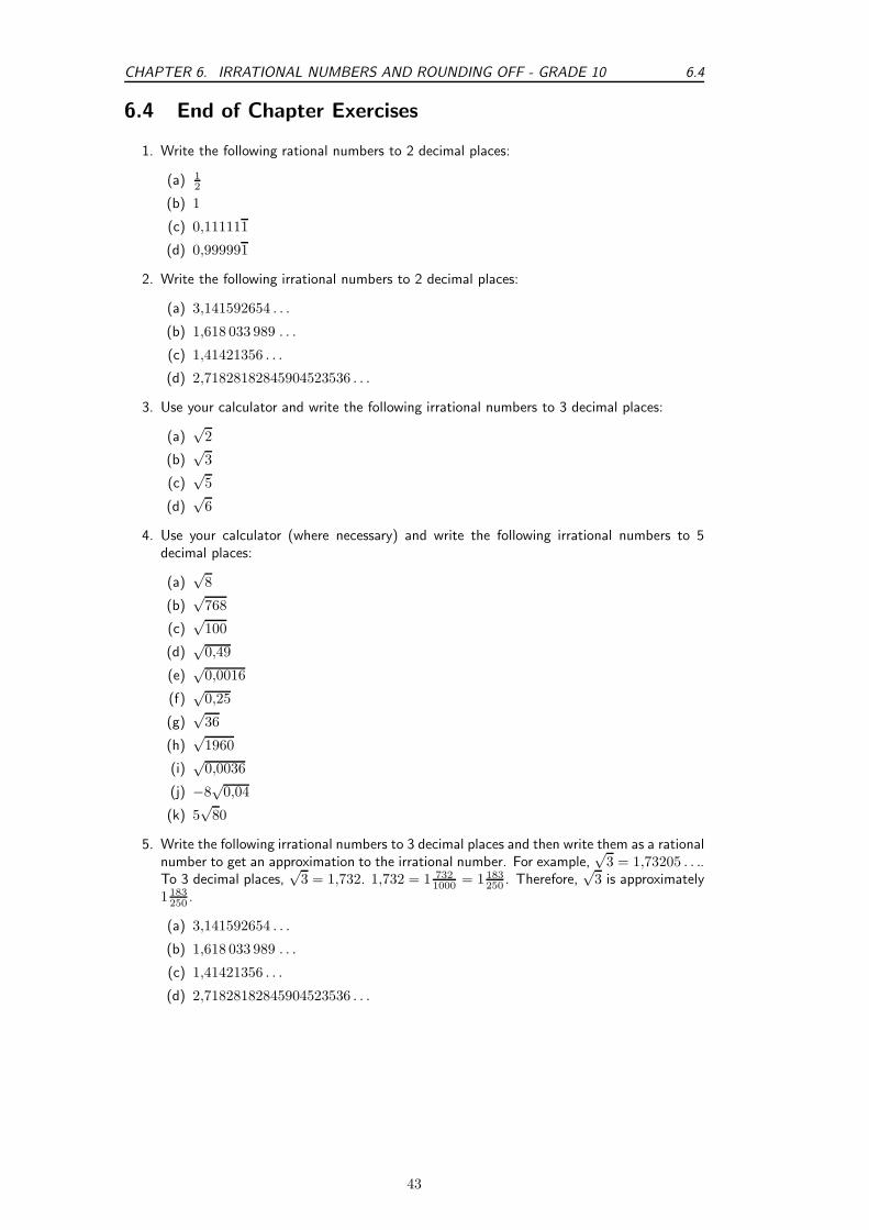
CHAPTER 6. IRRATIONAL NUMBERS AND ROUNDING OFF - GRADE 10 6.4
6.4 End of Chapter Exercises
1. Write the following rational numbers to 2 decimal places:
(a) 12
(b) 1
(c) 0,111111
(d) 0,999991
2. Write the following irrational numbers to 2 decimal places:
(a) 3,141592654 . . .
(b) 1,618 033 989 . . .
(c) 1,41421356 . . .
(d) 2,71828182845904523536 . . .
3. Use your calculator and write the following irrational numbers to 3 decimal places:
(a)√
2
(b)√
3
(c)√
5
(d)√
6
4. Use your calculator (where necessary) and write the following irrational numbers to 5decimal places:
(a)√
8
(b)√
768
(c)√
100
(d)√
0,49
(e)√
0,0016
(f)√
0,25
(g)√
36
(h)√
1960
(i)√
0,0036
(j) −8√
0,04
(k) 5√
80
5. Write the following irrational numbers to 3 decimal places and then write them as a rationalnumber to get an approximation to the irrational number. For example,
√3 = 1,73205 . . ..
To 3 decimal places,√
3 = 1,732. 1,732 = 1 7321000 = 1 183
250 . Therefore,√
3 is approximately1 183
250 .
(a) 3,141592654 . . .
(b) 1,618 033 989 . . .
(c) 1,41421356 . . .
(d) 2,71828182845904523536 . . .
43

6.4 CHAPTER 6. IRRATIONAL NUMBERS AND ROUNDING OFF - GRADE 10
44

Chapter 7
Number Patterns - Grade 10
In earlier grades you saw patterns in the form of pictures and numbers. In this chapter we learnmore about the mathematics of patterns.Patterns are recognisable regularities in situations suchas in nature, shapes, events, sets of numbers. For example, spirals on a pineapple, snowflakes,geometric designs on quilts or tiles, the number sequence 0, 4, 8, 12, 16,....
Activity :: Investigation : PatternsCan you spot any patterns in the following lists of numbers?
1. 2; 4; 6; 8; 10; . . .
2. 1; 2; 4; 7; 11; . . .
3. 1; 4; 9; 16; 25; . . .
4. 5; 10; 20; 40; 80; . . .
7.1 Common Number Patterns
Numbers can have interesting patterns. Here we list the most common patterns and how theyare made.
Examples:
1. 1, 4, 7, 10, 13, 16, 19, 22, 25, ...
This sequence has a difference of 3 between each number. The pattern is continued byadding 3 to the last number each time.
2. 3, 8, 13, 18, 23, 28, 33, 38, ...
This sequence has a difference of 5 between each number. The pattern is continued byadding 5 to the last number each time.
3. 2, 4, 8, 16, 32, 64, 128, 256, ...
This sequence has a factor of 2 between each number. The pattern is continued bymultiplying the last number by 2 each time.
4. 3, 9, 27, 81, 243, 729, 2187, ...
This sequence has a factor of 3 between each number. The pattern is continued bymultiplying the last number by 3 each time.
45

7.2 CHAPTER 7. NUMBER PATTERNS - GRADE 10
7.1.1 Special Sequences
Triangular Numbers
1, 3, 6, 10, 15, 21, 28, 36, 45, ...
This sequence is generated from a pattern of dots which form a triangle. By adding another rowof dots and counting all the dots we can find the next number of the sequence.
Square Numbers
1, 4, 9, 16, 25, 36, 49, 64, 81, ...
The next number is made by squaring where it is in the pattern. The second number is 2 squared(22 or 2 × 2) The seventh number is 7 squared (72 or 7 × 7) etc
Cube Numbers
1, 8, 27, 64, 125, 216, 343, 512, 729, ...
The next number is made by cubing where it is in the pattern. The second number is 2 cubed(23 or 2 × 2 × 2) The seventh number is 7 cubed (73 or 7 × 7 × 7) etc
Fibonacci Numbers
0, 1, 1, 2, 3, 5, 8, 13, 21, 34, ...
The next number is found by adding the two numbers before it together. The 2 is found byadding the two numbers in front of it (1 + 1) The 21 is found by adding the two numbers infront of it (8 + 13) The next number in the sequence above would be 55 (21 + 34)
Can you figure out the next few numbers?
7.2 Make your own Number Patterns
You can make your own number patterns using coins or matchsticks. Here is an example usingdots:
b
b b
b b
bb
b b b
b b b
b b b
b
b
b
b
b
b
b b b b
b b b b
b b b b
b b b b
b
b
b
b
b
b
b
b
b
b
bb
b
1 dot 6 dots 15 dots 28 dots
Pattern 1 2 3 4
46

CHAPTER 7. NUMBER PATTERNS - GRADE 10 7.3
How many dots would you need for pattern 5 ? Can you make a formula that will tell you howmany coins are needed for any size pattern? For example if the pattern 20? The formula maylook something like
dots = pattern × pattern + ...
Worked Example 5: Study Table
Question: Say you and 3 friends decide to study for Maths, and you are seated ata square table. A few minutes later, 2 other friends join you and would like to sit atyour table and help you study. Naturally, you move another table and add it to theexisting one. Now six of you sit at the table. Another two of your friends join yourtable, and you take a third table and add it to the existing tables. Now 8 of you cansit comfortably.
Figure 7.1: Two more people can be seated for each table added.
Examine how the number of people sitting is related to the number of tables.
Answer
Step 1 : Tabulate a few terms to see if there is a pattern
Number of Tables, n Number of people seated
1 4 = 42 4 + 2 = 63 4 + 2 + 2 = 84 4 + 2 + 2 + 2 = 10...
...n 4 + 2 + 2 + 2 + . . . + 2
Step 2 : Describe the pattern
We can see for 3 tables we can seat 8 people, for 4 tables we can seat 10 people andso on. We started out with 4 people and added two the whole time. Thus, for eachtable added, the number of persons increases by two.
7.3 Notation
A sequence does not have to follow a pattern but when it does we can often write down a formulato calculate the nth-term, an. In the sequence
1; 4; 9; 16; 25; . . .
where the sequence consists of the squares of integers, the formula for the nth-term is
an = n2 (7.1)
47

7.3 CHAPTER 7. NUMBER PATTERNS - GRADE 10
You can check this by looking at:
a1 = 12 = 1
a2 = 22 = 4
a3 = 32 = 9
a4 = 42 = 16
a5 = 52 = 25
. . .
Therefore, using (7.1), we can generate a pattern, namely squares of integers.
Worked Example 6: Study Table continued ....
Question: As before, you and 3 friends are studying for Maths, and you are seatedat a square table. A few minutes later, 2 other friends join you move another tableand add it to the existing one. Now six of you sit at the table. Another two of yourfriends join your table, and you take a third table and add it to the existing tables.Now 8 of you sit comfortably as illustrated:
Figure 7.2: Two more people can be seated for each table added.
Find the expression for the number of people seated at n tables. Then, use thegeneral formula to determine how many people can sit around 12 tables and howmany tables are needed for 20 people.AnswerStep 1 : Tabulate a few terms to see if there is a pattern
Number of Tables, n Number of people seated Formula
1 4 = 4 = 4 + 2 · (0)2 4 + 2 = 6 = 4 + 2 · (1)3 4 + 2 + 2 = 8 = 4 + 2 · (2)4 4 + 2 + 2 + 2 = 10 = 4 + 2 · (3)...
......
n 4 + 2 + 2 + 2 + . . . + 2 = 4 + 2 · (n − 1)
Step 2 : Describe the patternThe number of people seated at n tables is:
an = 4 + 2 · (n − 1)
Step 3 : Calculate the 12th termUsing the general formula (36.1) and considering the example from the previoussection, how many people can sit around, say, 12 tables? We are looking for a12,that is, where n = 12:
an = a1 + d · (n − 1)
a12 = 4 + 2 · (12 − 1)
= 4 + 2(11)
= 4 + 22
= 26
48

CHAPTER 7. NUMBER PATTERNS - GRADE 10 7.3
Step 4 : Calculate the number of terms if an = 20
an = a1 + d · (n − 1)
20 = 4 + 2 · (n − 1)
20 − 4 = 2 · (n − 1)
16 ÷ 2 = n − 1
8 + 1 = n
n = 9
Step 5 : Final Answer
26 people can be seated at 12 tables and 9 tables are needed to seat 20 people.
It is also important to note the difference between n and an. n can be compared to a placeholder, while an is the value at the place “held” by n. Like our “Study Table”-example above,the first table (Table 1) holds 4 people. Thus, at place n = 1, the value of a1 = 4, and so on:
n 1 2 3 4 . . .an 4 6 8 10 . . .
Activity :: Investigation : General Formula
1. Find the general formula for the following sequences and then find a10, a50 anda100:
(a) 2, 5, 8, 11, 14, . . .
(b) 0, 4, 8, 12, 16, . . .
(c) 2,−1,−4,−7,−10, . . .
2. The general term has been given for each sequence below. Work out the missingterms.
(a) 0; 3; ...; 15; 24 n2 − 1
(b) 3; 2; 1; 0; ...; 2 −n + 4
(c) 11; ...; 7; ...; 3 −13 + 2n
7.3.1 Patterns and Conjecture
In mathematics, a conjecture is a mathematical statement which appears to be true, but hasnot been formally proven to be true under the rules of mathematics. Other words that have asimilar in meaning to conjecture are: hypothesis, theory, assumption and premise.For example: Make a conjecture about the next number based on the pattern 2; 6; 11; 17 : ...The numbers increase by 4, 5, and 6.Conjecture: The next number will increase by 7. So, it will be 17 + 7 or 24.
49

7.4 CHAPTER 7. NUMBER PATTERNS - GRADE 10
Worked Example 7: Number patterns
Question: Consider the following pattern.
12 + 1 = 22 − 2
22 + 2 = 32 − 3
32 + 3 = 42 − 4
42 + 4 = 52 − 5
1. Add another two rows to the end of the pattern.
2. Make a conjecture about this pattern. Write your conjecture in words.
3. Generalise your conjecture for this pattern (in other words, write your conjecturealgebraically).
4. Prove that your conjecture is true.
AnswerStep 1 : The next two rows
52 + 5 = 62 − 6
62 + 6 = 72 − 7
Step 2 : ConjectureSquaring a number and adding the same number gives the same result as squaringthe next number and subtracting that number.Step 3 : GeneraliseWe have chosen to use x here. You could choose any letter to generalise the pattern.
x2 + x = (x + 1)2 − (x + 1)
Step 4 : Proof
Left side : x2 + x
Right side : (x + 1)2 − (x + 1)
Right side = x2 + 2x + 1 − x − 1
= x2 + x
= left side
Therefore x2 + x = (x + 1)2 − (x + 1)
7.4 Exercises
1. Find the nth term for: 3, 7, 11, 15, . . .
2. Find the general term of the following sequences:
50

CHAPTER 7. NUMBER PATTERNS - GRADE 10 7.4
(a) −2,1,4,7, . . .
(b) 11, 15, 19, 23, . . .
(c) x − 1,2x + 5,5x + 1, . . .
(d) sequence with a3 = 7 and a8 = 15
(e) sequence with a4 = −8 and a10 = 10
3. The seating in a section of a sports stadium can be arranged so the first row has 15 seats,the second row has 19 seats, the third row has 23 seats and so on. Calculate how manyseats are in the row 25.
4. Consider the following pattern:
22 + 2 = 32 − 3
32 + 3 = 42 − 4
42 + 4 = 52 − 5
(a) Add at least two more rows to the pattern and check whether or not the patterncontinues to work.
(b) Describe in words any patterns that you have noticed.
(c) Try to generalise a rule using algebra i.e. find the general term for the pattern.
(d) Prove or disprove that this rule works for all values.
5. The profits of a small company for the last four years has been: R10 000, R15 000, R19 000and R23 000. If the pattern continues, what is the expected profit in the 10 years (i.e. inthe 14th year of the company being in business)?
6. A single square is made from 4 matchsticks. Two squares in a row needs 7 matchsticksand 3 squares in a row needs 10 matchsticks. Determine:
(a) the first term
(b) the common difference
(c) the formula for the general term
(d) how many matchsticks are in a row of 25 squares
7. You would like to start saving some money, but because you have never tried to save moneybefore, you have decided to start slowly. At the end of the first week you deposit R5 intoyour bank account. Then at the end of the second week you deposit R10 into your bankaccount. At the end of the third week you deposit R15. After how many weeks, do youdeposit R50 into your bank account?
8. A horizontal line intersects a piece of string at four points and divides it into five parts, asshown below.
b b b b
1
2
3
4
5
51

7.4 CHAPTER 7. NUMBER PATTERNS - GRADE 10
If the piece of string is intersected in this way by 19 parallel lines, each of which intersectsit at four points, find the number of parts into which the string will be divided.
52

Chapter 8
Finance - Grade 10
8.1 Introduction
Should you ever find yourself stuck with a mathematics question on a television quiz show, youwill probably wish you had remembered the how many even prime numbers there are between 1and 100 for the sake of R1 000 000. And who does not want to be a millionaire, right?
Welcome to the Grade 10 Finance Chapter, where we apply maths skills to everyday financialsituations that you are likely to face both now and along your journey to purchasing your firstprivate jet.
If you master the techniques in this chapter, you will grasp the concept of compound interest,and how it can ruin your fortunes if you have credit card debt, or make you millions if yousuccessfully invest your hard-earned money. You will also understand the effects of fluctuatingexchange rates, and its impact on your spending power during your overseas holidays!
8.2 Foreign Exchange Rates
Is $500 (”500 US dollars”) per person per night a good deal on a hotel in New York City? Thefirst question you will ask is “How much is that worth in Rands?”. A quick call to the local bankor a search on the Internet (for example on http://www.x-rates.com/) for the Dollar/Randexchange rate will give you a basis for assessing the price.
A foreign exchange rate is nothing more than the price of one currency in terms of another.For example, the exchange rate of 6,18 Rands/US Dollars means that $1 costs R6,18. In otherwords, if you have $1 you could sell it for R6,18 - or if you wanted $1 you would have to payR6,18 for it.
But what drives exchange rates, and what causes exchange rates to change? And how does thisaffect you anyway? This section looks at answering these questions.
8.2.1 How much is R1 really worth?
We can quote the price of a currency in terms of any other currency, but the US Dollar, BritishPounds Sterling or even the Euro are often used as a market standard. You will notice that thefinancial news will report the South African Rand exchange rate in terms of these three majorcurrencies.
So the South African Rand could be quoted on a certain date as 6,7040 ZAR per USD (i.e.$1,00 costs R6,7040), or 12,2374 ZAR per GBP. So if I wanted to spend $1 000 on a holidayin the United States of America, this would cost me R6 704,00; and if I wanted £1 000 for aweekend in London it would cost me R12 237,40.
This seems obvious, but let us see how we calculated that: The rate is given as ZAR per USD,or ZAR/USD such that $1,00 buys R6,7040. Therefore, we need to multiply by 1 000 to get the
53

8.2 CHAPTER 8. FINANCE - GRADE 10
Table 8.1: Abbreviations and symbols for some common currencies.
Currency Abbreviation Symbol
South African Rand ZAR RUnited States Dollar USD $British Pounds Sterling GBP £
Euro EUR e
number of Rands per $1 000.
Mathematically,
$1,00 = R6,0740
∴ 1 000 × $1,00 = 1 000 × R6,0740
= R6 074,00
as expected.
What if you have saved R10 000 for spending money for the same trip and you wanted to usethis to buy USD? How much USD could you get for this? Our rate is in ZAR/USD but we wantto know how many USD we can get for our ZAR. This is easy. We know how much $1,00 costsin terms of Rands.
$1,00 = R6,0740
∴$1,00
6,0740=
R6,0740
6,0740
$1,00
6,0740= R1,00
R1,00 = $1,00
6,0740
= $0,164636
As we can see, the final answer is simply the reciprocal of the ZAR/USD rate. Therefore, R10 000will get:
R1,00 = $1,00
6,0740
∴ 10 000 × R1,00 = 10 000 × $1,00
6,0740
= $1 646,36
We can check the answer as follows:
$1,00 = R6,0740
∴ 1 646,36× $1,00 = 1 646,36× R6,0740
= R10 000,00
Six of one and half a dozen of the other
So we have two different ways of expressing the same exchange rate: Rands per Dollar (ZAR/USD)and Dollar per Rands (USD/ZAR). Both exchange rates mean the same thing and express thevalue of one currency in terms of another. You can easily work out one from the other - theyare just the reciprocals of the other.
If the South African Rand is our Domestic (or home) Currency, we call the ZAR/USD rate a“direct” rate, and we call a USD/ZAR rate an “indirect” rate.
In general, a direct rate is an exchange rate that is expressed as units of Home Currency per
54
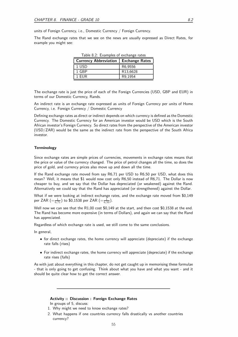
CHAPTER 8. FINANCE - GRADE 10 8.2
units of Foreign Currency, i.e., Domestic Currency / Foreign Currency.
The Rand exchange rates that we see on the news are usually expressed as Direct Rates, forexample you might see:
Table 8.2: Examples of exchange rates
Currency Abbreviation Exchange Rates
1 USD R6,95561 GBP R13,66281 EUR R9,1954
The exchange rate is just the price of each of the Foreign Currencies (USD, GBP and EUR) interms of our Domestic Currency, Rands.
An indirect rate is an exchange rate expressed as units of Foreign Currency per units of HomeCurrency, i.e. Foreign Currency / Domestic Currency
Defining exchange rates as direct or indirect depends on which currency is defined as the DomesticCurrency. The Domestic Currency for an American investor would be USD which is the SouthAfrican investor’s Foreign Currency. So direct rates from the perspective of the American investor(USD/ZAR) would be the same as the indirect rate from the perspective of the South Africainvestor.
Terminology
Since exchange rates are simple prices of currencies, movements in exchange rates means thatthe price or value of the currency changed. The price of petrol changes all the time, so does theprice of gold, and currency prices also move up and down all the time.
If the Rand exchange rate moved from say R6,71 per USD to R6,50 per USD, what does thismean? Well, it means that $1 would now cost only R6,50 instead of R6,71. The Dollar is nowcheaper to buy, and we say that the Dollar has depreciated (or weakened) against the Rand.Alternatively we could say that the Rand has appreciated (or strengthened) against the Dollar.
What if we were looking at indirect exchange rates, and the exchange rate moved from $0,149per ZAR (= 1
6,71 ) to $0,1538 per ZAR (= 16,50 ).
Well now we can see that the R1,00 cost $0,149 at the start, and then cost $0,1538 at the end.The Rand has become more expensive (in terms of Dollars), and again we can say that the Randhas appreciated.
Regardless of which exchange rate is used, we still come to the same conclusions.
In general,
• for direct exchange rates, the home currency will appreciate (depreciate) if the exchangerate falls (rises)
• For indirect exchange rates, the home currency will appreciate (depreciate) if the exchangerate rises (falls)
As with just about everything in this chapter, do not get caught up in memorising these formulae- that is only going to get confusing. Think about what you have and what you want - and itshould be quite clear how to get the correct answer.
Activity :: Discussion : Foreign Exchange RatesIn groups of 5, discuss:
1. Why might we need to know exchange rates?
2. What happens if one countries currency falls drastically vs another countriescurrency?
55

8.2 CHAPTER 8. FINANCE - GRADE 10
3. When might you use exchange rates?
8.2.2 Cross Currency Exchange Rates
We know that the exchange rates are the value of one currency expressed in terms of anothercurrency, and we can quote exchange rates against any other currency. The Rand exchange rateswe see on the news are usually expressed against the major currency, USD, GBP and EUR.
So if for example, the Rand exchange rates were given as 6,71 ZAR/USD and 12,71 ZAR/GBP,does this tell us anything about the exchange rate between USD and GBP?
Well I know that if $1 will buy me R6,71, and if £1.00 will buy me R12,71, then surely the GBPis stronger than the USD because you will get more Rands for one unit of the currency, and wecan work out the USD/GBP exchange rate as follows:
Before we plug in any numbers, how can we get a USD/GBP exchange rate from the ZAR/USDand ZAR/GBP exchange rates?
Well,USD/GBP = USD/ZAR × ZAR/GBP.
Note that the ZAR in the numerator will cancel out with the ZAR in the denominator, and weare left with the USD/GBP exchange rate.
Although we do not have the USD/ZAR exchange rate, we know that this is just the reciprocalof the ZAR/USD exchange rate.
USD/ZAR =1
ZAR/USD
Now plugging in the numbers, we get:
USD/GBP = USD/ZAR × ZAR/GBP
=1
ZAR/USD× ZAR/GBP
=1
6,71× 12,71
= 1,894
Important: Sometimes you will see exchange rates in the real world that do not appear towork exactly like this. This is usually because some financial institutions add other coststo the exchange rates, which alter the results. However, if you could remove the effect ofthose extra costs, the numbers would balance again.
Worked Example 8: Cross Exchange Rates
Question: If $1 = R 6,40, and £1 = R11,58 what is the $/£ exchange rate (i.e.the number of US$ per £)?AnswerStep 1 : Determine what is given and what is requiredThe following are given:
• ZAR/USD rate = R6,40
• ZAR/GBP rate = R11,58
56

CHAPTER 8. FINANCE - GRADE 10 8.2
The following is required:• USD/GBP rate
Step 2 : Determine how to approach the problemWe know that:
USD/GBP = USD/ZAR × ZAR/GBP.
Step 3 : Solve the problem
USD/GBP = USD/ZAR × ZAR/GBP
=1
ZAR/USD× ZAR/GBP
=1
6,40× 11,58
= 1,8094
Step 4 : Write the final answer$1,8094 can be bought for £1.
Activity :: Investigation : Cross Exchange Rates - Alternate MethodIf $1 = R 6,40, and £1 = R11,58 what is the $/£ exchange rate (i.e. the number
of US$ per £)?Overview of problemYou need the $/£ exchange rate, in other words how many dollars must you pay
for a pound. So you need £1. From the given information we know that it wouldcost you R11,58 to buy £1 and that $ 1 = R6,40.
Use this information to:1. calculate how much R1 is worth in $.
2. calculate how much R11,58 is worth in $.Do you get the same answer as in the worked example?
8.2.3 Enrichment: Fluctuating exchange rates
If everyone wants to buy houses in a certain suburb, then house prices are going to go up - becausethe buyers will be competing to buy those houses. If there is a suburb where all residents wantto move out, then there are lots of sellers and this will cause house prices in the area to fall -because the buyers would not have to struggle as much to find an eager seller.
This is all about supply and demand, which is a very important section in the study of Economics.You can think about this is many different contexts, like stamp-collecting for example. If thereis a stamp that lots of people want (high demand) and few people own (low supply) then thatstamp is going to be expensive.
And if you are starting to wonder why this is relevant - think about currencies. If you are goingto visit London, then you have Rands but you need to “buy” Pounds. The exchange rate is theprice you have to pay to buy those Pounds.
Think about a time where lots of South Africans are visiting the United Kingdom, and otherSouth Africans are importing goods from the United Kingdom. That means there are lots ofRands (high supply) trying to buy Pounds. Pounds will start to become more expensive (comparethis to the house price example at the start of this section if you are not convinced), and the
57

8.3 CHAPTER 8. FINANCE - GRADE 10
exchange rate will change. In other words, for R1 000 you will get fewer Pounds than you wouldhave before the exchange rate moved.
Another context which might be useful for you to understand this: consider what would happenif people in other countries felt that South Africa was becoming a great place to live, and thatmore people were wanting to invest in South Africa - whether in properties, businesses - or justbuying more goods from South Africa. There would be a greater demand for Rands - and the“price of the Rand” would go up. In other words, people would need to use more Dollars, orPounds, or Euros ... to buy the same amount of Rands. This is seen as a movement in exchangerates.
Although it really does come down to supply and demand, it is interesting to think about whatfactors might affect the supply (people wanting to “sell” a particular currency) and the demand(people trying to “buy” another currency). This is covered in detail in the study of Economics,but let us look at some of the basic issues here.
There are various factors affect exchange rates, some of which have more economic rationalethan others:
• economic factors (such as inflation figures, interest rates, trade deficit information, mon-etary policy and fiscal policy)
• political factors (such as uncertain political environment, or political unrest)
• market sentiments and market behaviour (for example if foreign exchange markets per-ceived a currency to be overvalued and starting selling the currency, this would cause thecurrency to fall in value - a self fulfilling expectation).
Exercise: Foreign Exchange
1. I want to buy an IPOD that costs £100, with the exchange rate currently at£1 = R14. I believe the exchange rate will reach R12 in a month.
(a) How much will the MP3 player cost in Rands, if I buy it now?
(b) How much will I save if the exchange rate drops to R12?
(c) How much will I lose if the exchange rate moves to R15?
2. Study the following exchange rate table:
Country Currency Exchange RateUnited Kingdom (UK) Pounds(£) R14,13United States (USA) Dollars ($) R7,04
(a) In South Africa the cost of a new Honda Civic is R173 400. In England thesame vehicle costs £12 200 and in the USA $ 21 900. In which country isthe car the cheapest if you compare it to the South African Rand ?
(b) Sollie and Arinda are waiters in a South African Restaurant attracting manytourists from abroad. Sollie gets a £6 tip from a tourist and Arinda gets$ 12. How many South African Rand did each one get ?
8.3 Being Interested in Interest
If you had R1 000, you could either keep it in your wallet, or deposit it in a bank account. If itstayed in your wallet, you could spend it any time you wanted. If the bank looked after it foryou, then they could spend it, with the plan of making profit off it. The bank usually “pays” youto deposit it into an account, as a way of encouraging you to bank it with them, This paymentis like a reward, which provides you with a reason to leave it with the bank for a while, ratherthan keeping the money in your wallet.
58

CHAPTER 8. FINANCE - GRADE 10 8.4
We call this reward ”interest”.
If you deposit money into a bank account, you are effectively lending money to the bank - andyou can expect to receive interest in return. Similarly, if you borrow money from a bank (or froma department store, or a car dealership, for example) then you can expect to have to pay intereston the loan. That is the price of borrowing money.
The concept is simple, yet it is core to the world of finance. Accountants, actuaries and bankers,for example, could spend their entire working career dealing with the effects of interest onfinancial matters.
In this chapter you will be introduced to the concept of financial mathematics - and given thetools to cope with even advanced concepts and problems.
Important: Interest
The concepts in this chapter are simple - we are just looking at the same idea, but from manydifferent angles. The best way to learn from this chapter is to do the examples yourself, as youwork your way through. Do not just take our word for it!
8.4 Simple Interest
Definition: Simple InterestSimple interest is where you earn interest on the initial amount that you invested, but notinterest on interest.
As an easy example of simple interest, consider how much you will get by investing R1 000 for1 year with a bank that pays you 5% simple interest. At the end of the year, you will get aninterest of:
Interest = R1 000 × 5%
= R1 000 × 5
100= R1 000 × 0,05
= R50
So, with an “opening balance” of R1 000 at the start of the year, your “closing balance” at theend of the year will therefore be:
Closing Balance = Opening Balance + Interest
= R1 000 + R50
= R1 050
We sometimes call the opening balance in financial calculations Principal, which is abbreviatedas P (R1 000 in the example). The interest rate is usually labelled i (5% in the example), andthe interest amount (in Rand terms) is labelled I (R50 in the example).
So we can see that:I = P × i (8.1)
and
Closing Balance = Opening Balance + Interest
= P + I
= P + (P × i)
= P (1 + i)
59

8.4 CHAPTER 8. FINANCE - GRADE 10
This is how you calculate simple interest. It is not a complicated formula, which is just as wellbecause you are going to see a lot of it!
Not Just One
You might be wondering to yourself:
1. how much interest will you be paid if you only leave the money in the account for 3 months,or
2. what if you leave it there for 3 years?
It is actually quite simple - which is why they call it Simple Interest.
1. Three months is 1/4 of a year, so you would only get 1/4 of a full year’s interest, whichis: 1/4 × (P × i). The closing balance would therefore be:
Closing Balance = P + 1/4 × (P × i)
= P (1 + (1/4)i)
2. For 3 years, you would get three years’ worth of interest, being: 3 × (P × i). The closingbalance at the end of the three year period would be:
Closing Balance = P + 3 × (P × i)
= P × (1 + (3)i)
If you look carefully at the similarities between the two answers above, we can generalise theresult. In other words, if you invest your money (P ) in an account which pays a rate of interest(i) for a period of time (n years), then, using the symbol (A) for the Closing Balance:
Closing Balance,(A) = P (1 + i · n) (8.2)
As we have seen, this works when n is a fraction of a year and also when n covers several years.
Important: Interest Calculation
Annual Rates means Yearly rates. and p.a.(per annum) = per year
Worked Example 9: Simple Interest
Question: If I deposit R1 000 into a special bank account which pays a SimpleInterest of 7% for 3 years, how much will I get back at the end?AnswerStep 1 : Determine what is given and what is required
• opening balance, P = R1 000
• interest rate, i = 7%
• period of time, n = 3 yearsWe are required to find the closing balance (A).Step 2 : Determine how to approach the problemWe know from (8.2) that:
Closing Balance,(A) = P (1 + i · n)
60

CHAPTER 8. FINANCE - GRADE 10 8.4
Step 3 : Solve the problem
A = P (1 + i · n)
= R1 000(1 + 3 × 7%)
= R1 210
Step 4 : Write the final answer
The closing balance after 3 years of saving R1 000 at an interest rate of 7% is R1 210.
Worked Example 10: Calculating n
Question: If I deposit R30 000 into a special bank account which pays a SimpleInterest of 7.5% ,for how many years must I invest this amount to generate R45 000
Answer
Step 1 : Determine what is given and what is required
• opening balance, P = R30 000
• interest rate, i = 7,5%
• closing balance, A = R45 000
We are required to find the number of years.
Step 2 : Determine how to approach the problem
We know from (8.2) that:
Closing Balance (A) = P (1 + i · n)
Step 3 : Solve the problem
Closing Balance (A) = P (1 + i · n)
R45 000 = R30 000(1 + n × 7,5%)
(1 + 0,075 × n) =45000
300000,075× n = 1,5 − 1
n =0,5
0,075n = 6,6666667
Step 4 : Write the final answer
n has to be a whole number, therefore n = 7.The period is 7 years for R30 000 to generate R45 000 at a simple interest rate of7,5%.
8.4.1 Other Applications of the Simple Interest Formula
61

8.4 CHAPTER 8. FINANCE - GRADE 10
Worked Example 11: Hire-Purchase
Question: Troy is keen to buy an addisional hard drive for his laptop advertised forR 2 500 on the internet. There is an option of paying a 10% deposit then making24 monthly payments using a hire-purchase agreement where interest is calculatedat 7,5% p.a. simple interest. Calculate what Troy’s monthly payments will be.AnswerStep 1 : Determine what is given and what is requiredA new opening balance is required, as the 10% deposit is paid in cash.
• 10% of R 2 500 = R250
• new opening balance, P = R2 500 − R250 = R2 250
• interest rate, i = 7,5% = 0,075pa
• period of time, n = 2 years
We are required to find the closing balance (A) and then the montly payments.Step 2 : Determine how to approach the problemWe know from (8.2) that:
Closing Balance,(A) = P (1 + i · n)
Step 3 : Solve the problem
A = P (1 + i · n)
= R2 250(1 + 2 × 7,5%)
= R2 587,50
Monthly payment = 2587,50÷ 24
= R107,81
Step 4 : Write the final answerTroy’s monthly payments = R 107,81
Worked Example 12: Depreciation
Question: Seven years ago, Tjad’s drum kit cost him R12 500. It has now beenvalued at R2 300. What rate of simple depreciation does this represent ?AnswerStep 1 : Determine what is given and what is required
• opening balance, P = R12 500
• period of time, n = 7 years
• closing balance, A = R2 300
We are required to find the rate(i).Step 2 : Determine how to approach the problemWe know from (8.2) that:
Closing Balance,(A) = P (1 + i · n)
Therefore, for depreciation the formula will change to:
Closing Balance,(A) = P (1 − i · n)
62

CHAPTER 8. FINANCE - GRADE 10 8.5
Step 3 : Solve the problem
A = P (1 − i · n)
R2 300 = R12 500(1− 7 × i)
i = 0,11657...
Step 4 : Write the final answerTherefore the rate of depreciation is 11,66%
Exercise: Simple Interest
1. An amount of R3 500 is invested in a savings account which pays simple interestat a rate of 7,5% per annum. Calculate the balance accumulated by the endof 2 years.
2. Calculate the simple interest for the following problems.
(a) A loan of R300 at a rate of 8% for l year.
(b) An investment of R225 at a rate of 12,5% for 6 years.
3. I made a deposit of R5 000 in the bank for my 5 year old son’s 21st birthday.I have given him the amount of R 18 000 on his birtday. At what rate was themoney invested, if simple interest was calculated ?
4. Bongani buys a dining room table costing R 8 500 on Hire Purchase. He ischarged simple interest at 17,5% per annum over 3 years.
(a) How much will Bongani pay in total ?
(b) How much interest does he pay ?
(c) What is his montly installment ?
8.5 Compound Interest
To explain the concept of compound interest, the following example is discussed:
Worked Example 13: Using Simple Interest to lead to the concept Com-
pound InterestQuestion: If I deposit R1 000 into a special bank account which pays a SimpleInterest of 7%. What if I empty the bank account after a year, and then take theprincipal and the interest and invest it back into the same account again. Then Itake it all out at the end of the second year, and then put it all back in again? Andthen I take it all out at the end of 3 years?AnswerStep 1 : Determine what is given and what is required
• opening balance, P = R1 000
• interest rate, i = 7%
63

8.5 CHAPTER 8. FINANCE - GRADE 10
• period of time, 1 year at a time, for 3 yearsWe are required to find the closing balance at the end of three years.Step 2 : Determine how to approach the problemWe know that:
Closing Balance = P (1 + i · n)
Step 3 : Determine the closing balance at the end of the first year
Closing Balance = P (1 + i · n)
= R1 000(1 + 1 × 7%)
= R1 070
Step 4 : Determine the closing balance at the end of the second yearAfter the first year, we withdraw all the money and re-deposit it. The openingbalance for the second year is therefore R1 070, because this is the balance after thefirst year.
Closing Balance = P (1 + i · n)
= R1 070(1 + 1 × 7%)
= R1 144,90
Step 5 : Determine the closing balance at the end of the third yearAfter the second year, we withdraw all the money and re-deposit it. The openingbalance for the third year is therefore R1 144,90, because this is the balance afterthe first year.
Closing Balance = P (1 + i · n)
= R1 144,90(1 + 1 × 7%)
= R1 225,04
Step 6 : Write the final answerThe closing balance after withdrawing the all the money and re-depositing each yearfor 3 years of saving R1 000 at an interest rate of 7% is R1 225,04.
In the two worked examples using simple interest, we have basically the same problem becauseP=R1 000, i=7% and n=3 years for both problems. Except in the second situation, we end upwith R1 225,04 which is more than R1 210 from the first example. What has changed?
In the first example I earned R70 interest each year - the same in the first, second and third year.But in the second situation, when I took the money out and then re-invested it, I was actuallyearning interest in the second year on my interest (R70) from the first year. (And interest onthe interest on my interest in the third year!)
This more realistically reflects what happens in the real world, and is known as CompoundInterest. It is this concept which underlies just about everything we do - so we will look at moreclosely next.
Definition: Compound InterestCompound interest is the interest payable on the principal and its accumulated interest.
Compound interest is a double edged sword, though - great if you are earning interest on cashyou have invested, but crippling if you are stuck having to pay interest on money you haveborrowed!
In the same way that we developed a formula for Simple Interest, let us find one for CompoundInterest.
64

CHAPTER 8. FINANCE - GRADE 10 8.5
If our opening balance is P and we have an interest rate of i then, the closing balance at theend of the first year is:
Closing Balance after 1 year = P (1 + i)
This is the same as Simple Interest because it only covers a single year. Then, if we take thatout and re-invest it for another year - just as you saw us doing in the worked example above -then the balance after the second year will be:
Closing Balance after 2 years = [P (1 + i)] × (1 + i)
= P (1 + i)2
And if we take that money out, then invest it for another year, the balance becomes:
Closing Balance after 3 years = [P (1 + i)2] × (1 + i)
= P (1 + i)3
We can see that the power of the term (1 + i) is the same as the number of years. Therefore,
Closing Balance after n years = P (1 + i)n (8.3)
8.5.1 Fractions add up to the Whole
It is easy to show that this formula works even when n is a fraction of a year. For example, letus invest the money for 1 month, then for 4 months, then for 7 months.
Closing Balance after 1 month = P (1 + i)112
Closing Balance after 5 months = Closing Balance after 1 month invested for 4 months more
= [P (1 + i)112 ]
412
= P (1 + i)112
+ 412
= P (1 + i)512
Closing Balance after 12 months = Closing Balance after 5 month invested for 7 months more
= [P (1 + i)512 ]
712
= P (1 + i)512
+ 712
= P (1 + i)1212
= P (1 + i)1
which is the same as investing the money for a year.
Look carefully at the long equation above. It is not as complicated as it looks! All we are doingis taking the opening amount (P ), then adding interest for just 1 month. Then we are takingthat new balance and adding interest for a further 4 months, and then finally we are taking thenew balance after a total of 5 months, and adding interest for 7 more months. Take a lookagain, and check how easy it really is.
Does the final formula look familiar? Correct - it is the same result as you would get for simplyinvesting P for one full year. This is exactly what we would expect, because:
1 month + 4 months + 7 months = 12 months,
which is a year. Can you see that? Do not move on until you have understood this point.
8.5.2 The Power of Compound Interest
To see how important this “interest on interest” is, we shall compare the difference in closingbalances for money earning simple interest and money earning compound interest. Consider anamount of R10 000 that you have to invest for 10 years, and assume we can earn interest of 9%.How much would that be worth after 10 years?
65

8.5 CHAPTER 8. FINANCE - GRADE 10
The closing balance for the money earning simple interest is:
Closing Balance = P (1 + i · n)
= R10 000(1 + 9% × 10)
= R19 000
The closing balance for the money earning compound interest is:
Closing Balance = P (1 + i)n)
= R10 000(1 + 9%)10
= R23 673,64
So next time someone talks about the “magic of compound interest”, not only will you knowwhat they mean - but you will be able to prove it mathematically yourself!
Again, keep in mind that this is good news and bad news. When you are earning interest onmoney you have invested, compound interest helps that amount to increase exponentially. Butif you have borrowed money, the build up of the amount you owe will grow exponentially too.
Worked Example 14: Taking out a Loan
Question: Mr Lowe wants to take out a loan of R 350 000. He does not wantto pay back more than R625 000 altogether on the loan. If the interest rate he isoffered is 13%, over what period should he take the loanAnswerStep 1 : Determine what has been provided and what is required
• opening balance, P = R350 000
• closing balance, A = R625 000
• interest rate, i = 13% peryear
We are required to find the time period(n).Step 2 : Determine how to approach the problemWe know from (8.3) that:
Closing Balance,(A) = P (1 + i)n
We need to find n.Therefore we covert the formula to:
A
P= (1 + i)n
and then find n by trial and error.Step 3 : Solve the problem
A
P= (1 + i)n
625000
350000= (1 + 0,13)n
1,785... = (1,13)n
Try n = 3 : (1,13)3 = 1,44...
Try n = 4 : (1,13)4 = 1,63...
Try n = 5 : (1,13)5 = 1,84...
Step 4 : Write the final answerMr Lowe should take the loan over four years
66

CHAPTER 8. FINANCE - GRADE 10 8.5
8.5.3 Other Applications of Compound Growth
Worked Example 15: Population Growth
Question: South Africa’s population is increasing by 2,5% per year. If the currentpopulation is 43 million, how many more people will there be in South Africa in twoyear’s time ?AnswerStep 1 : Determine what has been provided and what is required
• opening balance, P = 43 000 000
• period of time, n = 2 year
• interest rate, i = 2,5% peryear
We are required to find the closing balance(A).Step 2 : Determine how to approach the problemWe know from (8.3) that:
Closing Balance,(A) = P (1 + i)n
Step 3 : Solve the problem
A = P (1 + i)n
= 43 000 000(1 + 0,025)2
= 45 176 875
Step 4 : Write the final answerThere are 45 176 875 − 43 000 000 = 2 176 875 more people in 2 year’s time
Worked Example 16: Compound Decrease
Question: A swimming pool is being treated for a build-up of algae. Initially, 50m2
of the pool is covered by algae. With each day of treatment, the algae reduces by5%. What area is covered by algae after 30 days of treatment ?AnswerStep 1 : Determine what has been provided and what is required
• opening balance, P = 50m2
• period of time, n = 30 days
• interest rate, i = 5% perday
We are required to find the closing balance(A).Step 2 : Determine how to approach the problemWe know from (8.3) that:
Closing Balance,(A) = P (1 + i)n
67

8.6 CHAPTER 8. FINANCE - GRADE 10
But this is compound decrease so we can use the formula:
Closing Balance,(A) = P (1 − i)n
Step 3 : Solve the problem
A = P (1 − i)n
= 50(1 − 0,05)30
= 10,73m2
Step 4 : Write the final answerTherefore the area still covered with algae is 10,73m2
Exercise: Compound Interest
1. An amount of R3 500 is invested in a savings account which pays compoundinterest at a rate of 7,5% per annum. Calculate the balance accumulated bythe end of 2 years.
2. If the average rate of inflation for the past few years was 7,3% and your waterand electricity account is R 1 425 on average, what would you expect to payin 6 years time ?
3. Shrek wants to invest some money at 11% per annum compound interest. Howmuch money (to the nearest rand) should he invest if he wants to reach a sumof R 100 000 in five year’s time ?
8.6 Summary
As an easy reference, here are the key formulae that we derived and used during this chapter.While memorising them is nice (there are not many), it is the application that is useful. Financialexperts are not paid a salary in order to recite formulae, they are paid a salary to use the rightmethods to solve financial problems.
8.6.1 Definitions
P Principal (the amount of money at the starting point of the calculation)i interest rate, normally the effective rate per annumn period for which the investment is made
8.6.2 Equations
Closing Balance - simple interestSolve for iSolve for n
= P (1 + i · n)
68

CHAPTER 8. FINANCE - GRADE 10 8.7
Closing Balance - compound interestSolve for iSolve for n
= P (1 + i)n
Important: Always keep the interest and the time period in the same units of time (e.g.both in years, or both in months etc.).
8.7 End of Chapter Exercises
1. You are going on holiday to Europe. Your hotel will cost e200 per night. How much willyou need in Rands to cover your hotel bill, if the exchange rate is e1 = R9,20.
2. Calculate how much you will earn if you invested R500 for 1 year at the following interestrates:
(a) 6,85% simple interest
(b) 4,00% compound interest
3. Bianca has R1 450 to invest for 3 years. Bank A offers a savings account which payssimple interest at a rate of 11% per annum, whereas Bank B offers a savings accountpaying compound interest at a rate of 10,5% per annum. Which account would leaveBianca with the highest accumulated balance at the end of the 3 year period?
4. How much simple interest is payable on a loan of R2 000 for a year, if the interest rate is10%?
5. How much compound interest is payable on a loan of R2 000 for a year, if the interest rateis 10%?
6. Discuss:
(a) Which type of interest would you like to use if you are the borrower?
(b) Which type of interest would you like to use if you were the banker?
7. Calculate the compound interest for the following problems.
(a) A R2 000 loan for 2 years at 5%.
(b) A R1 500 investment for 3 years at 6%.
(c) An R800 loan for l year at 16%.
8. If the exchange rate 100 Yen = R 6,2287 and 1 AUD = R 5,1094 , determine the exchangerate between the Australian Dollar and the Japanese Yen.
9. Bonnie bought a stove for R 3 750. After 3 years she paid for it and the R 956,25 interestthat was charged for hire-purchase. Determine the simple rate of interest that was charged.
69

8.7 CHAPTER 8. FINANCE - GRADE 10
70

Chapter 9
Products and Factors - Grade 10
9.1 Introduction
In this chapter you will learn how to work with algebraic expressions. You will recap some ofthe work on factorisation and multiplying out expressions that you learnt in earlier grades. Thiswork will then be extended upon for Grade 10.
9.2 Recap of Earlier Work
The following should be familiar. Examples are given as reminders.
9.2.1 Parts of an Expression
Mathematical expressions are just like sentences and their parts have special names. You shouldbe familiar with the following names used to describe the parts of an mathematical expression.
a · xk + b · x + cm = 0 (9.1)
d · yp + e · y + f ≤ 0 (9.2)
Name Examples (separated by commas)
term a · xk ,b · x, cm, d · yp, e · y, f
expression a · xk + b · x + cm, d · yp + e · y + fcoefficient a, b, d, eexponent (or index) k, pbase x, y, cconstant a, b, c, d, e, fvariable x, y
equation a · xk + b · x + cm = 0inequality d · yp + e · y + f ≤ 0binomial expression with two termstrinomial expression with three terms
9.2.2 Product of Two Binomials
A binomial is a mathematical expression with two terms, e.g. (ax + b) and (cx + d). If thesetwo binomials are multiplied, the following is the result:
71

9.2 CHAPTER 9. PRODUCTS AND FACTORS - GRADE 10
(a · x + b)(c · x + d) = (ax)(c · x + d) + b(c · x + d)
= (ax)(cx) + (ax)d + b(cx) + b · d
Worked Example 17: Product of two Binomials
Question: Find the product of (3x − 2)(5x + 8)Answer
(3x − 2)(5x + 8) = (3x)(5x) + (3x)(8) + (−2)(5x) + (−2)(8)
= 15x2 + 24x − 10x − 16
= 15x2 + 14x − 16
The product of two identical binomials is known as the square of the binomials and is writtenas:
(ax + b)2 = a2x2 + 2abx + b2
If the two terms are ax + b and ax − b then their product is:
(ax + b)(ax − b) = a2x2 − b2
This is known as the difference of squares.
9.2.3 Factorisation
Factorisation is the opposite of expanding brackets. For example expanding brackets wouldrequire 2(x+ 1) to be written as 2x+2. Factorisation would be to start with 2x+2 and to endup with 2(x + 1). In previous grades you factorised based on common factors and on differenceof squares.
Common Factors
Factorising based on common factors relies on there being common factors between your terms.For example, 2x − 6x2 can be factorised as follows:
2x − 6x2 = 2x(1 − 3x)
Activity :: Investigation : Common FactorsFind the highest common factors of the following pairs of terms:
(a) 6y; 18x (b) 12mn; 8n (c) 3st; 4su (d) 18kl; 9kp (e) abc; ac(f) 2xy; 4xyz (g) 3uv; 6u (h) 9xy; 15xz (i) 24xyz; 16yz (j) 3m; 45n
72

CHAPTER 9. PRODUCTS AND FACTORS - GRADE 10 9.2
Difference of Squares
We have seen that:(ax + b)(ax − b) = a2x2 − b2 (9.3)
Since 9.3 is an equation, both sides are always equal. This means that an expression of the form:
a2x2 − b2
can be factorised to(ax + b)(ax − b)
Therefore,a2x2 − b2 = (ax + b)(ax − b)
For example, x2 − 16 can be written as (x2 − 42) which is a difference of squares. Therefore thefactors of x2 − 16 are (x − 4) and (x + 4).
Worked Example 18: Factorisation
Question: Factorise completely: b2y5 − 3aby3
Answer
b2y5 − 3aby3 = by3(by2 − 3a)
Worked Example 19: Factorising binomials with a common bracket
Question: Factorise completely: 3a(a − 4) − 7(a − 4)AnswerStep 1 : bracket (a − 4) is the common factor
3a(a − 4) − 7(a − 4) = (a − 4)(3a − 7)
Worked Example 20: Factorising using a switch around in brackets
Question: Factorise 5(a − 2) − b(2 − a)AnswerStep 1 : Note that (2 − a) = −(a − 2)
5(a − 2) − b(2 − a) = 5(a − 2) − [−b(a− 2)]
= 5(a − 2) + b(a − 2)
= (a − 2)(5 + b)
73

9.3 CHAPTER 9. PRODUCTS AND FACTORS - GRADE 10
Exercise: Recap
1. Find the products of:
(a) 2y(y + 4) (b) (y + 5)(y + 2) (c) (y + 2)(2y + 1)(d) (y + 8)(y + 4) (e) (2y + 9)(3y + 1) (f) (3y − 2)(y + 6)
2. Factorise:
(a) 2l + 2w
(b) 12x + 32y
(c) 6x2 + 2x + 10x3
(d) 2xy2 + xy2z + 3xy
(e) −2ab2 − 4a2b
3. Factorise completely:
(a) 7a + 4 (b) 20a − 10 (c) 18ab − 3bc(d) 12kj + 18kq (e) 16k2 − 4k (f) 3a2 + 6a − 18(g) −6a − 24 (h) −2ab − 8a (i) 24kj − 16k2j(j) −a2b − b2a (k) 12k2j + 24k2j2 (l) 72b2q − 18b3q2
(m) 4(y − 3) + k(3− y) (n) a(a − 1) − 5(a − 1) (o) bm(b+4)−6m(b+4)(p) a2(a+7)+ a(a+7) (q) 3b(b− 4)− 7(4− b) (r) a2b2c2 − 1
9.3 More Products
We have seen how to multiply two binomials in section 9.2.2. In this section we learn how tomultiply a binomial (expression with two terms) by a trinomial (expression with three terms).Fortunately, we use the same methods we used to multiply two binomials to multiply a binomialand a trinomial.
For example, multiply 2x + 1 by x2 + 2x + 1.
(2x + 1)(x2 + 2x + 1)
= 2x(x2 + 2x + 1) + 1(x2 + 2x + 1) (apply distributive law)
= [2x(x2) + 2x(2x) + 2x(1)] + [1(x2) + 1(2x) + 1(1)]
= 4x3 + 4x2 + 2x + x2 + 2x + 1 (expand the brackets)
= 4x3 + (4x2 + x2) + (2x + 2x) + 1 (group like terms to simplify)
= 4x3 + 5x2 + 4x + 1 (simplify to get final answer)
Important: Multiplication of Binomial with Trinomial
If the binomial is A + B and the trinomial is C + D + E, then the very first step is to apply thedistributive law:
(A + B)(C + D + E) = A(C + D + E) + B(C + D + E) (9.4)
If you remember this, you will never go wrong!
74

CHAPTER 9. PRODUCTS AND FACTORS - GRADE 10 9.3
Worked Example 21: Multiplication of Binomial with Trinomial
Question: Multiply x − 1 with x2 − 2x + 1.
Answer
Step 1 : Determine what is given and what is required
We are given two expressions: a binomial, x − 1, and a trinomial, x2 − 2x + 1. Weneed to multiply them together.
Step 2 : Determine how to approach the problem
Apply the distributive law and then simplify the resulting expression.
Step 3 : Solve the problem
(x − 1)(x2 − 2x + 1)
= x(x2 − 2x + 1) − 1(x2 − 2x + 1) (apply distributive law)
= [x(x2) + x(−2x) + x(1)] + [−1(x2) − 1(−2x) − 1(1)]
= x3 − 2x2 + x − x2 + 2x − 1 (expand the brackets)
= x3 + (−2x2 − x2) + (x + 2x) − 1 (group like terms to simplify)
= x3 − 3x2 + 3x − 1 (simplify to get final answer)
Step 4 : Write the final answer
The product of x − 1 and x2 − 2x + 1 is x3 − 3x2 + 3x − 1.
Worked Example 22: Sum of Cubes
Question: Find the product of x + y and x2 − xy + y2.
Answer
Step 1 : Determine what is given and what is required
We are given two expressions: a binomial, x + y, and a trinomial, x2 −xy + y2. Weneed to multiply them together.
Step 2 : Determine how to approach the problem
Apply the distributive law and then simplify the resulting expression.
Step 3 : Solve the problem
(x + y)(x2 − xy + y2)
= x(x2 − xy + y2) + y(x2 − xy + y2) (apply distributive law)
= [x(x2) + x(−xy) + x(y2)] + [y(x2) + y(−xy) + y(y2)]
= x3 − x2y + xy2 + yx2 − xy2 + y3 (expand the brackets)
= x3 + (−x2y + yx2) + (xy2 − xy2) + y3 (group like terms to simplify)
= x3 + y3 (simplify to get final answer)
Step 4 : Write the final answer
The product of x + y and x2 − xy + y2 is x3 + y3.
75

9.4 CHAPTER 9. PRODUCTS AND FACTORS - GRADE 10
Important: We have seen that:
(x + y)(x2 − xy + y2) = x3 + y3
This is known as a sum of cubes.
Activity :: Investigation : Difference of CubesShow that the difference of cubes (x3 − y3) is given by the product of x− y and
x2 + xy + y2.
Exercise: Products
1. Find the products of:
(a) (−2y2 − 4y + 11)(5y − 12) (b) (−11y + 3)(−10y2 − 7y − 9)(c) (4y2 + 12y + 10)(−9y2 + 8y + 2) (d) (7y2 − 6y − 8)(−2y + 2)(e) (10y5 + 3)(−2y2 − 11y + 2) (f) (−12y − 3)(12y2 − 11y + 3)(g) (−10)(2y2 + 8y + 3) (h) (2y6 + 3y5)(−5y − 12)(i) (6y7 − 8y2 + 7)(−4y − 3)(−6y2 − 7y − 11) (j) (−9y2 + 11y + 2)(8y2 + 6y − 7)(k) (8y5 + 3y4 + 2y3)(5y + 10)(12y2 + 6y + 6) (l) (−7y + 11)(−12y + 3)(m) (4y3 +5y2−12y)(−12y−2)(7y2−9y+12) (n) (7y + 3)(7y2 + 3y + 10)(o) (9)(8y2 − 2y + 3) (p) (−12y + 12)(4y2 − 11y + 11)(q) (−6y4 + 11y2 + 3y)(10y + 4)(4y − 4) (r) (−3y6 − 6y3)(11y − 6)(10y − 10)(s) (−11y5 + 11y4 + 11)(9y3 − 7y2 − 4y + 6) (t) (−3y + 8)(−4y3 + 8y2 − 2y + 12)
2. Remove the brackets and simplify:(2h + 3)(4h2 − 6h + 9)
9.4 Factorising a Quadratic
Finding the factors of a quadratic is quite easy, and some are easier than others.
The simplest quadratic has the form ax2, which factorises to (x)(ax). For example, 25x2
factorises to (5x)(5x) and 2x2 factorises to (2x)(x).
The second simplest quadratic is of the form ax2 + bx. We can see here that x is a commonfactor of both terms. Therefore, ax2 + bx factorises to x(ax + b). For example, 8y2 + 4yfactorises to 4y(2y + 1).
The third simplest quadratic is made up of the difference of squares. We know that:
(a + b)(a − b) = a2 − b2.
This is true for any values of a and b, and more importantly since it is an equality, we can alsowrite:
a2 − b2 = (a + b)(a − b).
This means that if we ever come across a quadratic that is made up of a difference of squares,we can immediately write down what the factors are.
76

CHAPTER 9. PRODUCTS AND FACTORS - GRADE 10 9.4
Worked Example 23: Difference of Squares
Question: Find the factors of 9x2 − 25.AnswerStep 1 : Examine the quadraticWe see that the quadratic is a difference of squares because:
(3x)2 = 9x2
and52 = 25.
Step 2 : Write the quadratic as the difference of squares
9x2 − 25 = (3x)2 − 52
Step 3 : Write the factors
(3x)2 − 52 = (3x − 5)(3x + 5)
Step 4 : Write the final answerThe factors of 9x2 − 25 are (3x − 5)(3x + 5).
The three types of quadratic that we have seen are very simple to factorise. However, manyquadratics do not fall into these categories, and we need a more general method to factorisequadratics like x2 − x − 2?
We can learn about how to factorise quadratics by looking at how two binomials are multipliedto get a quadratic. For example, (x + 2)(x + 3) is multiplied out as:
(x + 2)(x + 3) = x(x + 3) + 2(x + 3)
= (x)(x) + 3x + 2x + (2)(3)
= x2 + 5x + 6.
We see that the x2 term in the quadratic is the product of the x-terms in each bracket. Similarly,the 6 in the quadratic is the product of the 2 and 3 the brackets. Finally, the middle term is thesum of two terms.
So, how do we use this information to factorise the quadratic?
Let us start with factorising x2 +5x+6 and see if we can decide upon some general rules. Firstly,write down two brackets with an x in each bracket and space for the remaining terms.
( x )( x )
Next decide upon the factors of 6. Since the 6 is positive, these are:
Factors of 6
1 62 3-1 -6-2 -3
Therefore, we have four possibilities:
Option 1 Option 2 Option 3 Option 4(x + 1)(x + 6) (x − 1)(x − 6) (x + 2)(x + 3) (x − 2)(x − 3)
77

9.4 CHAPTER 9. PRODUCTS AND FACTORS - GRADE 10
Next we expand each set of brackets to see which option gives us the correct middle term.
Option 1 Option 2 Option 3 Option 4(x + 1)(x + 6) (x − 1)(x − 6) (x + 2)(x + 3) (x − 2)(x − 3)x2 + 7x + 6 x2 − 7x + 6 x2 + 5x + 6 x2 − 5x + 6
We see that Option 3 (x+2)(x+3) is the correct solution. As you have seen that the processof factorising a quadratic is mostly trial and error, however the is some information that can beused to simplify the process.
Method: Factorising a Quadratic
1. First divide the entire equation by any common factor of the coefficients, so as to obtainan equation of the form ax2 + bx + c = 0 where a, b and c have no common factors anda is positive.
2. Write down two brackets with an x in each bracket and space for the remaining terms.
( x )( x ) (9.5)
3. Write down a set of factors for a and c.
4. Write down a set of options for the possible factors for the quadratic using the factors ofa and c.
5. Expand all options to see which one gives you the correct answer.
There are some tips that you can keep in mind:
• If c is positive, then the factors of c must be either both positive or both negative. Thefactors are both negative if b is negative, and are both positive if b is positive. If c isnegative, it means only one of the factors of c is negative, the other one being positive.
• Once you get an answer, multiply out your brackets again just to make sure it really works.
Worked Example 24: Factorising a Quadratic
Question: Find the factors of 3x2 + 2x − 1.AnswerStep 1 : Check whether the quadratic is in the form ax2 + bx + c = 0 with apositive.The quadratic is in the required form.Step 2 : Write down two brackets with an x in each bracket and space forthe remaining terms.
( x )( x ) (9.6)
Write down a set of factors for a and c. The possible factors for a are: (1,3).The possible factors for c are: (-1,1) or (1,-1).
Write down a set of options for the possible factors for the quadratic using thefactors of a and c. Therefore, there are two possible options.
Option 1 Option 2(x − 1)(3x + 1) (x + 1)(3x − 1)3x2 − 2x − 1 3x2 + 2x − 1
78

CHAPTER 9. PRODUCTS AND FACTORS - GRADE 10 9.5
Step 3 : Check your answer
(x + 1)(3x − 1) = x(3x − 1) + 1(3x − 1)
= (x)(3x) + (x)(−1) + (1)(3x) + (1)(−1)
= 3x2 − x + 3x − 1
= x2 + 2x − 1.
Step 4 : Write the final answerThe factors of 3x2 + 2x − 1 are (x + 1) and (3x − 1).
Exercise: Factorising a Trinomial
1. Factorise the following:
(a) x2 + 8x + 15 (b) x2 + 10x + 24 (c) x2 + 9x + 8(d) x2 + 9x + 14 (e) x2 + 15x + 36 (f) x2 + 13x + 36
2. Factorise the following:
(a) x2 − 2x − 15
(b) x2 + 2x − 3
(c) x2 + 2x − 8
(d) x2 + x − 20
(e) x2 − x − 20
3. Find the factors for the following quadratic expressions:
(a) 2x2 + 11x + 5
(b) 3x2 + 19x + 6
(c) 6x2 + 7x + 2
(d) 12x2 + 7x + 1
(e) 8x2 + 6x + 1
4. Find the factors for the following trinomials:
(a) 3x2 + 17x − 6
(b) 7x2 − 6x − 1
(c) 8x2 − 6x + 1
(d) 2x2 − 5x − 3
9.5 Factorisation by Grouping
One other method of factorisation involves the use of common factors. We know that the factorsof 3x + 3 are 3 and (x + 1). Similarly, the factors of 2x2 + 2x are 2x and (x + 1). Therefore, ifwe have an expression:
2x2 + 2x + 3x + 3
then we can factorise as:2x(x + 1) + 3(x + 1).
You can see that there is another common factor: x + 1. Therefore, we can now write:
(x + 1)(2x + 3).
We get this by taking out the x + 1 and see what is left over. We have a +2x from the firstterm and a +3 from the second term. This is called factorisation by grouping.
79

9.6 CHAPTER 9. PRODUCTS AND FACTORS - GRADE 10
Worked Example 25: Factorisation by Grouping
Question: Find the factors of 7x + 14y + bx + 2by by groupingAnswerStep 1 : Determine if there are common factors to all termsThere are no factors that are common to all terms.Step 2 : Determine if there are factors in common between some terms7 is a common factor of the first two terms and b is a common factor of the secondtwo terms.Step 3 : Re-write expression taking the factors into account
7x + 14y + bx + 2by = 7(x + 2y) + b(x + 2y)
Step 4 : Determine if there are more common factorsx + 2y is a common factor.Step 5 : Re-write expression taking the factors into account
7(x + 2y) + b(x + 2y) = (x + 2y)(7 + b)
Step 6 : Write the final answerThe factors of 7x + 14y + bx + 2by are (7 + b) and (x + 2y).
Exercise: Factorisation by Grouping
1. Factorise by grouping: 6x + 9 + 2ax + 3
2. Factorise by grouping: x2 − 6x + 5x − 30
3. Factorise by grouping: 5x + 10y − ax − 2ay
4. Factorise by grouping: a2 − 2a − ax + 2x
5. Factorise by grouping: 5xy − 3y + 10x − 6
9.6 Simplification of Fractions
In some cases of simplifying an algebraic expression, the expression will be a fraction. Forexample,
x2 + 3x
x + 3
has a quadratic in the numerator and a binomial in the denominator. You can apply the differentfactorisation methods to simplify the expression.
x2 + 3x
x + 3
=x(x + 3)
x + 3= x provided x 6= −3
80

CHAPTER 9. PRODUCTS AND FACTORS - GRADE 10 9.6
Worked Example 26: Simplification of Fractions
Question: Simplify: 2x−b+x−abax2−abx
Answer
Step 1 : Factorise numerator and denominator
Use grouping for numerator and common factor for denominator in this example.
=(ax − ab) + (x − b)
ax2 − abx
=a(x − b) + (x − b)
ax(x − b)
=(x − b)(a + 1)
ax(x − b)
Step 2 : Cancel out same factors
The simplified answer is:
=a + 1
ax
Worked Example 27: Simplification of Fractions
Question: Simplify:x2−x−2x2−4 ÷ x2+x
x2+2x
Answer
Step 1 : Factorise numerators and denominators
=(x + 1)(x − 2)
(x + 2)(x − 2)÷ x(x + 1)
x(x + 2)
Step 2 : Multiply by factorised reciprocal
=(x + 1)(x − 2)
(x + 2)(x − 2)× x(x + 2)
x(x + 1)
Step 3 : Cancel out same factors
The simplified answer is
= 1
Exercise: Simplification of Fractions
1. Simplify:
81

9.7 CHAPTER 9. PRODUCTS AND FACTORS - GRADE 10
(a) 3a15 (b) 2a+10
4
(c) 5a+20a+4 (d) a2−4a
a−4
(e) 3a2−9a2a−6 (f) 9a+27
9a+18
(g) 6ab+2a2b
(h) 16x2y−8xy12x−6
(i) 4xyp−8xp12xy
(j) 3a+914 ÷ 7a+21
a+3
(k) a2−5a2a+10 ÷ 3a+15
4a(l) 3xp+4p
8p÷ 12p2
3x+4
(x) 162xp+4x
÷ 6x2+8x12 (y) 24a−8
12 ÷ 9a−36
(o) a2+2a5 ÷ 2a+4
20 (p) p2+pq7p
÷ 8p+8q21q
(q) 5ab−15b4a−12 ÷ 6b2
a+b(r) f2a−fa2
f−a
2. Simplify: x2−13 × 1
x−1 − 12
9.7 End of Chapter Exercises
1. Factorise:
(a) a2 − 9 (b) m2 − 36 (c) 9b2 − 81(d) 16b6 − 25a2 (e) m2 − (1/9) (f) 5 − 5a2b6
(g) 16ba4 − 81b (h) a2 − 10a + 25 (i) 16b2 + 56b + 49(j) 2a2 − 12ab + 18b2 (k) −4b2−144b8+48b5 (l) a3 − 27(m) 125a3 + b3 (n) 128b7 − 250ba6 (o) c3 + 27(p) 64b3 + 1 (q) 5a3 − 40c3 (r) 2b4 − 128b
2. Show that (2x − 1)2 − (x − 3)2 can be simplified to (x + 2)(3x − 4)
3. What must be added to x2 − x + 4 to make it equal to (x + 2)2
82

Chapter 10
Equations and Inequalities - Grade10
10.1 Strategy for Solving Equations
This chapter is all about solving different types of equations for one or two variables. In general,we want to get the unknown variable alone on the left hand side of the equation with all theconstants on the right hand side of the equation. For example, in the equation x − 1 = 0, wewant to be able to write the equation as x = 1.
As we saw in section 2.9 (page 13), an equation is like a set of weighing scales, that must alwaysbe balanced. When we solve equations, we need to keep in mind that what is done to one sidemust be done to the other.
Method: Rearranging Equations
You can add, subtract, multiply or divide both sides of an equation by any number you want, aslong as you always do it to both sides.
For example, in the equation x+5−1 = −6, we want to get x alone on the left hand side of theequation. This means we need to subtract 5 and add 1 on the left hand side. However, becausewe need to keep the equation balanced, we also need to subtract 5 and add 1 on the right handside.
x + 5 − 1 = −6
x + 5 − 5 − 1 + 1 = −6 − 5 + 1
x + 0 + 0 = −11 + 1
x = −10
In another example, 23x = 8, we must divide by 2 and multiply by 3 on the left hand side in
order to get x alone. However, in order to keep the equation balanced, we must also divide by2 and multiply by 3 on the right hand side.
2
3x = 8
2
3x ÷ 2 × 3 = 8 ÷ 2 × 3
2
2× 3
3× x =
8 × 3
21 × 1 × x = 12
x = 12
These are the basic rules to apply when simplifying any equation. In most cases, these ruleshave to be applied more than once, before we have the unknown variable on the left hand side
83

10.2 CHAPTER 10. EQUATIONS AND INEQUALITIES - GRADE 10
of the equation.
We are now ready to solve some equations!
Important: The following must also be kept in mind:
1. Division by 0 is undefined.
2. If xy
= 0, then x = 0 and y 6= 0, because division by 0 is undefined.
Activity :: Investigation : Strategy for Solving Equations
In the following, identify what is wrong.
4x − 8 = 3(x − 2)
4(x − 2) = 3(x − 2)
4(x − 2)
(x − 2)=
3(x − 2)
(x − 2)
4 = 3
10.2 Solving Linear Equations
The simplest equation to solve is a linear equation. A linear equation is an equation where thepower on the variable(letter, e.g. x) is 1(one). The following are examples of linear equations.
2x + 2 = 12 − x
3x + 1= 2
4
3x − 6 = 7x + 2
In this section, we will learn how to find the value of the variable that makes both sides of thelinear equation true. For example, what value of x makes both sides of the very simple equation,x + 1 = 1 true.
Since the highest power on the variable is one(1) in a linear equation, there is at most onesolution or root for the equation.
This section relies on all the methods we have already discussed: multiplying out expressions,grouping terms and factorisation. Make sure that you are comfortable with these methods,before trying out the work in the rest of this chapter.
2x + 2 = 1
2x = 1 − 2 (like terms together)
2x = −1 (simplified as much a possible)
Now we see that 2x = −1. This means if we divide both sides by 2, we will get:
x = −1
284

CHAPTER 10. EQUATIONS AND INEQUALITIES - GRADE 10 10.2
If we substitute x = − 12 , back into the original equation, we get:
2x + 2
= 2(−1
2) + 2
= −1 + 2
= 1
That is all that there is to solving linear equations.
Important: Solving Equations
When you have found the solution to an equation, substitute the solution into the originalequation, to check your answer.
Method: Solving Equations
The general steps to solve equations are:
1. Expand(Remove) all brackets.
2. ”Move” all terms with the variable to the left hand side of equation, and all constant terms(the numbers) to the right hand side of the equal to-sign. Bearing in mind that the signof the terms will chance(from (+) to (-) or vice versa, as they ”cross over” the equal tosign.
3. Group all like terms together and simplify as much as possible.
4. Factorise if necessary.
5. Find the solution.
6. Substitute solution into original equation to check answer.
Worked Example 28: Solving Linear Equations
Question: Solve for x: 4 − x = 4AnswerStep 1 : Determine what is given and what is requiredWe are given 4 − x = 4 and are required to solve for x.Step 2 : Determine how to approach the problemSince there are no brackets, we can start with grouping like terms and then simpli-fying.Step 3 : Solve the problem
4 − x = 4
−x = 4 − 4 (move all constant terms (numbers) to the RHS (right hand side))
−x = 0 (group like terms together)
−x = 0 (simplify grouped terms)
−x = 0
∴ x = 0
Step 4 : Check the answer
85

10.2 CHAPTER 10. EQUATIONS AND INEQUALITIES - GRADE 10
Substitute solution into original equation:
4 − 0 = 4
4 = 4
Since both sides are equal, the answer is correct.Step 5 : Write the Final AnswerThe solution of 4 − x = 4 is x = 0.
Worked Example 29: Solving Linear Equations
Question: Solve for x: 4(2x − 9) − 4x = 4 − 6xAnswerStep 1 : Determine what is given and what is requiredWe are given 4(2x − 9) − 4x = 4 − 6x and are required to solve for x.Step 2 : Determine how to approach the problemWe start with expanding the brackets, then grouping like terms and then simplifying.Step 3 : Solve the problem
4(2x − 9) − 4x = 4 − 6x
8x − 36 − 4x = 4 − 6x (expand the brackets)
8x − 4x + 6x = 4 + 36 (move all terms with x to the LHS and all constant terms to the RHS of the =)
(8x − 4x + 6x) = (4 + 36) (group like terms together)
10x = 40 (simplify grouped terms)
10
10x =
40
10(divide both sides by 10)
x = 4
Step 4 : Check the answerSubstitute solution into original equation:
4(2(4) − 9) − 4(4) = 4 − 6(4)
4(8 − 9) − 16 = 4 − 24
4(−1)− 16 = −20
−4 − 16 = −20
−20 = −20
Since both sides are equal to −20, the answer is correct.Step 5 : Write the Final AnswerThe solution of 4(2x − 9) − 4x = 4 − 6x is x = 4.
Worked Example 30: Solving Linear Equations
Question: Solve for x: 2−x3x+1 = 2
Answer
86

CHAPTER 10. EQUATIONS AND INEQUALITIES - GRADE 10 10.2
Step 1 : Determine what is given and what is requiredWe are given 2−x
3x+1 = 2 and are required to solve for x.Step 2 : Determine how to approach the problemSince there is a denominator of (3x+1), we can start by multiplying both sides ofthe equation by (3x+1). But because division by 0 is not permissible, there is arestriction on a value for x. (x 6= −1
3 )Step 3 : Solve the problem
2 − x
3x + 1= 2
(2 − x) = 2(3x + 1)
2 − x = 6x + 2 (remove/expand brackets)
−x − 6x = 2 − 2 (move all terms containing x to the LHS and all constant terms (numbers) to the RHS.)
−7x = 0 (simplify grouped terms)
x = 0 ÷ (−7)
therefore x = 0 zero divide by any number is 0
Step 4 : Check the answerSubstitute solution into original equation:
2 − (0)
3(0) + 1= 2
2
1= 2
Since both sides are equal to 2, the answer is correct.
Step 5 : Write the Final AnswerThe solution of 2−x
3x+1 = 2 is x = 0.
Worked Example 31: Solving Linear Equations
Question: Solve for x: 43x − 6 = 7x + 2
AnswerStep 1 : Determine what is given and what is requiredWe are given 4
3x − 6 = 7x + 2 and are required to solve for x.Step 2 : Determine how to approach the problemWe start with multiplying each of the terms in the equation by 3, then grouping liketerms and then simplifying.Step 3 : Solve the problem
4
3x − 6 = 7x + 2
4x − 18 = 21x + 6 (each term is multiplied by 3
4x − 21x = 6 + 18 (move all terms with x to the LHS and all constant terms to the RHS of the =)
−17x = 24 (simplify grouped terms)
−17
−17x =
24
−17(divide both sides by -17)
x =−24
1787

10.2 CHAPTER 10. EQUATIONS AND INEQUALITIES - GRADE 10
Step 4 : Check the answer
Substitute solution into original equation:
4
3× −24
17− 6 = 7 × −24
17+ 2
4 × (−8)
(17)− 6 =
7 × (−24)
17+ 2
(−32)
17− 6 =
−168
17+ 2
−32 − 102
17=
(−168) + 34
17−134
17=
−134
17
Since both sides are equal to −13417 , the answer is correct.
Step 5 : Write the Final Answer
The solution of 43x − 6 = 7x + 2 is, x = −24
17 .
Exercise: Solving Linear Equations
1. Solve for y: 2y − 3 = 7
2. Solve for w: −3w = 0
3. Solve for z: 4z = 16
4. Solve for t: 12t + 0 = 144
5. Solve for x: 7 + 5x = 62
6. Solve for y: 55 = 5y + 34
7. Solve for z: 5z = 3z + 45
8. Solve for a: 23a− 12 = 6 + 2a
9. Solve for b: 12 − 6b + 34b = 2b − 24 − 64
10. Solve for c: 6c + 3c = 4 − 5(2c− 3).
11. Solve for p: 18 − 2p = p + 9
12. Solve for q: 4q
= 1624
13. Solve for q: 41 = q
2
14. Solve for r: −(−16− r) = 13r − 1
15. Solve for d: 6d − 2 + 2d = −2 + 4d + 8
16. Solve for f : 3f − 10 = 10
17. Solve for v: 3v + 16 = 4v − 10
18. Solve for k: 10k + 5 + 0 = −2k + −3k + 80
19. Solve for j: 8(j − 4) = 5(j − 4)
20. Solve for m: 6 = 6(m + 7) + 5m
88

CHAPTER 10. EQUATIONS AND INEQUALITIES - GRADE 10 10.3
10.3 Solving Quadratic Equations
A quadratic equation is an equation where the power on the variable is at most 2. The followingare examples of quadratic equations.
2x2 + 2x = 12 − x
3x + 1= 2x
4
3x − 6 = 7x2 + 2
Quadratic equations differ from linear equations by the fact that a linear equation only has onesolution, while a quadratic equation has at most two solutions. There are some special situationswhen a quadratic equation only has one solution.
We solve quadratic equations by factorisation, that is writing the quadratic as a product of twoexpressions in brackets. For example, we know that:
(x + 1)(2x − 3) = 2x2 − x − 3.
In order to solve:2x2 − x − 3 = 0
we need to be able to write 2x2 − x − 3 as (x + 1)(2x− 3), which we already know how to do.
Activity :: Investigation : Factorising a QuadraticFactorise the following quadratic expressions:
1. x + x2
2. x2 + 1 + 2x
3. x2 − 4x + 5
4. 16x2 − 9
5. 4x2 + 4x + 1
Being able to factorise a quadratic means that you are one step away from solving a quadraticequation. For example, x2 − 3x − 2 = 0 can be written as (x − 1)(x − 2) = 0. This meansthat both x − 1 = 0 and x − 2 = 0, which gives x = 1 and x = 2 as the two solutions to thequadratic equation x2 − 3x − 2 = 0.
Method: Solving Quadratic Equations
1. First divide the entire equation by any common factor of the coefficients, so as to obtainan equation of the form ax2 + bx + c = 0 where a, b and c have no common factors. Forexample, 2x2 + 4x + 2 = 0 can be written as x2 + 2x + 1 = 0 by dividing by 2.
2. Write ax2 + bx + c in terms of its factors (rx + s)(ux + v).This means (rx + s)(ux + v) = 0.
3. Once writing the equation in the form (rx + s)(ux + v) = 0, it then follows that the twosolutions are x = − s
ror x = −u
v.
Extension: Solutions of Quadratic EquationsThere are two solutions to a quadratic equation, because any one of the values cansolve the equation.
89

10.3 CHAPTER 10. EQUATIONS AND INEQUALITIES - GRADE 10
Worked Example 32: Solving Quadratic Equations
Question: Solve for x: 3x2 + 2x − 1 = 0AnswerStep 1 : Find the factors of 3x2 + 2x − 1As we have seen the factors of 3x2 + 2x − 1 are (x + 1) and (3x − 1).Step 2 : Write the equation with the factors
(x + 1)(3x − 1) = 0
Step 3 : Determine the two solutionsWe have
x + 1 = 0
or3x − 1 = 0
Therefore, x = −1 or x = 13 .
Step 4 : Write the final answer3x2 + 2x − 1 = 0 for x = −1 or x = 1
3 .
Worked Example 33: Solving Quadratic Equations
Question: Solve for x:√
x + 2 = xAnswerStep 1 : Square both sides of the equationBoth sides of the equation should be squared to remove the square root sign.
x + 2 = x2
Step 2 : Write equation in the form ax2 + bx + c = 0
x + 2 = x2 (subtract x2 to both sides)
x + 2 − x2 = 0 (divide both sides by -1)
−x − 2 + x2 = 0
x2 − x + 2 = 0
Step 3 : Factorise the quadratic
x2 − x + 2
The factors of x2 − x + 2 are (x − 2)(x + 1).
Step 4 : Write the equation with the factors
(x − 2)(x + 1) = 0
Step 5 : Determine the two solutionsWe have
x + 1 = 0
orx − 2 = 0
90

CHAPTER 10. EQUATIONS AND INEQUALITIES - GRADE 10 10.3
Therefore, x = −1 or x = 2.
Step 6 : Check whether solutions are valid
Substitute x = −1into the original equation√
x + 2 = x:
LHS =√
(−1) + 2
=√
1
= 1
but
RHS = (−1)
Therefore LHS6=RHSTherefore x 6= −1Now substitute x = 2 into original equation
√x + 2 = x:
LHS =√
2 + 2
=√
4
= 2
and
RHS = 2
Therefore LHS = RHSTherefore x = 2 is the only valid solution
Step 7 : Write the final answer√x + 2 = x for x = 2 only.
Worked Example 34: Solving Quadratic Equations
Question: Solve the equation: x2 + 3x − 4 = 0.
Answer
Step 1 : Check if the equation is in the form ax2 + bx + c = 0
The equation is in the required form, with a = 1.
Step 2 : Factorise the quadratic
You need the factors of 1 and 4 so that the middle term is +3 So the factors are:(x − 1)(x + 4)
Step 3 : Solve the quadratic equation
x2 + 3x − 4 = (x − 1)(x + 4) = 0 (10.1)
Therefore x = 1 or x = −4.
Step 4 : Write the final solution
Therefore the solutions are x = 1 or x = −4.
91

10.3 CHAPTER 10. EQUATIONS AND INEQUALITIES - GRADE 10
Worked Example 35: Solving Quadratic Equations
Question: Find the roots of the quadratic equation 0 = −2x2 + 4x − 2.AnswerStep 1 : Determine whether the equation is in the form ax2 + bx + c = 0,with no common factors.There is a common factor: -2. Therefore, divide both sides of the equation by -2.
−2x2 + 4x − 2 = 0
x2 − 2x + 1 = 0
Step 2 : Factorise x2 − 2x + 1The middle term is negative. Therefore, the factors are (x − 1)(x − 1)If we multiply out (x − 1)(x − 1), we get x2 − 2x + 1.Step 3 : Solve the quadratic equation
x2 − 2x + 1 = (x − 1)(x − 1) = 0
In this case, the quadratic is a perfect square, so there is only one solution for x:x = 1.Step 4 : Write the final solutionThe root of 0 = −2x2 + 4x − 2 is x = 1.
Exercise: Solving Quadratic Equations
1. Solve for x: (3x + 2)(3x − 4) = 0
2. Solve for a: (5a − 9)(a + 6) = 0
3. Solve for x: (2x + 3)(2x − 3) = 0
4. Solve for x: (2x + 1)(2x − 9) = 0
5. Solve for x: (2x − 3)(2x − 3) = 0
6. Solve for x: 20x + 25x2 = 0
7. Solve for a: 4a2 − 17a− 77 = 0
8. Solve for x: 2x2 − 5x − 12 = 0
9. Solve for b: −75b2 + 290b − 240 = 0
10. Solve for y: 2y = 13y2 − 3y + 14 2
3
11. Solve for θ: θ2 − 4θ = −4
12. Solve for q: −q2 + 4q − 6 = 4q2 − 5q + 3
13. Solve for t: t2 = 3t
14. Solve for w: 3w2 + 10w − 25 = 0
15. Solve for v: v2 − v + 3
16. Solve for x: x2 − 4x + 4 = 0
17. Solve for t: t2 − 6t = 7
18. Solve for x: 14x2 + 5x = 6
19. Solve for t: 2t2 − 2t = 12
20. Solve for y: 3y2 + 2y − 6 = y2 − y + 2
92

CHAPTER 10. EQUATIONS AND INEQUALITIES - GRADE 10 10.4
10.4 Exponential Equations of the form ka(x+p) = m
examples solved by trial and error)
Exponential equations generally have the unknown variable as the power. The following areexamples of exponential equations:
2x = 12−x
3x+1= 2
4
3− 6 = 7x + 2
You should already be familiar with exponential notation. Solving exponential equations aresimple, if we remember how to apply the laws of exponentials.
Activity :: Investigation : Solving Exponential EquationsSolve the following equations by completing the table:
2x = 2 x-3 -2 -1 0 1 2 3
2x
3x = 9 x-3 -2 -1 0 1 2 3
3x
2x+1 = 8 x-3 -2 -1 0 1 2 3
2x+1
10.4.1 Algebraic Solution
Definition: Equality for Exponential FunctionsIf a is a positive number such that a > 0, then:
ax = ay
if and only if:x = y
.
This means that if we can write all terms in an equation with the same base, we can solve theexponential equations by equating the indices. For example take the equation 3x+1 = 9. Thiscan be written as:
3x+1 = 32.
Since the bases are equal (to 3), we know that the exponents must also be equal. Therefore wecan write:
x + 1 = 2.
This gives:x = 1.
93

10.4 CHAPTER 10. EQUATIONS AND INEQUALITIES - GRADE 10
Method: Solving Exponential Equations
Try to write all terms with the same base.
Activity :: Investigation : Exponential NumbersWrite the following with the same base. The base is the first in the list. For
example, in the list 2, 4, 8, the base is two and we can write 4 as 22.
1. 2,4,8,16,32,64,128,512,1024
2. 3,9,27,81,243
3. 5,25,125,625
4. 13,169
5. 2x, 4x2, 8x3, 49x8
Worked Example 36: Solving Exponential Equations
Question: Solve for x: 2x = 2AnswerStep 1 : Try to write all terms with the same base.All terms are written with the same base.
2x = 21
Step 2 : Equate the indices
x = 1
Step 3 : Check your answer
2x
= 2(1)
= 21
Since both sides are equal, the answer is correct.Step 4 : Write the final answer
x = 1
is the solution to 2x = 2.
Worked Example 37: Solving Exponential Equations
Question: Solve:2x+4 = 42x
94

CHAPTER 10. EQUATIONS AND INEQUALITIES - GRADE 10 10.4
AnswerStep 1 : Try to write all terms with the same base.
2x+4 = 42x
2x+4 = 22(2x)
2x+4 = 24x
Step 2 : Equate the indices
x + 4 = 4x
Step 3 : Solve for x
x + 4 = 4x
x − 4x = −4
−3x = −4
x =−4
−3
x =4
3
Step 4 : Check your answer
LHS = 2x+4
= 2( 43+4)
= 2163
= (216)13
RHS = 42x
= 42( 43)
= 483
= (48)13
= ((22)8)13
= (216)13
= LHS
Since both sides are equal, the answer is correct.Step 5 : Write the final answer
x =4
3
is the solution to 2x+4 = 42x.
Exercise: Solving Exponential Equations
1. Solve the following exponential equations.
a. 2x+5 = 25 b. 32x+1 = 33 c. 52x+2 = 53
d. 65−x = 612 e. 64x+1 = 162x+5 f. 125x = 5
2. Solve: 39x−2 = 27
95

10.5 CHAPTER 10. EQUATIONS AND INEQUALITIES - GRADE 10
3. Solve for k: 81k+2 = 27k+4
4. The growth of an algae in a pond is can be modeled by the function f(t) = 2t.Find the value of t such that f(t) = 128?
5. Solve for x: 25(1−2x) = 54
6. Solve for x: 27x × 9x−2 = 1
10.5 Linear Inequalities
graphically;
Activity :: Investigation : Inequalities on a Number LineRepresent the following on number lines:
1. x = 4
2. x < 4
3. x ≤ 4
4. x ≥ 4
5. x > 4
A linear inequality is similar to a linear equation and has the power on the variable is equal to 1.The following are examples of linear inequalities.
2x + 2 ≤ 12 − x
3x + 1≥ 2
4
3x − 6 < 7x + 2
The methods used to solve linear inequalities are identical to those used to solve linear equations.The only difference occurs when there is a multiplication or a division that involves a minus sign.For example, we know that 8 > 6. If both sides of the inequality are divided by −2, −4 is notgreater than −3. Therefore, the inequality must switch around, making −4 < −3.
Important: When you divide or multiply both sides of an inequality by any number with aminus sign, the direction of the inequality changes.
For example, if x < 1, then −x > −1.
In order to compare am inequality to a normal equation, we shall solve an equation first. Solve2x + 2 = 1.
2x + 2 = 1
2x = 1 − 2
2x = −1
x = −1
2
If we represent this answer on a number line, we get
96

CHAPTER 10. EQUATIONS AND INEQUALITIES - GRADE 10 10.5
b
-3 -2 -1 0 1 2 3
x = − 12
Now let us solve the inequality 2x + 2 ≤ 1.
2x + 2 ≤ 1
2x ≤ 1 − 2
2x ≤ −1
x ≤ −1
2
If we represent this answer on a number line, we get
b
-3 -2 -1 0 1 2 3
x ≤ − 12
As you can see, for the equation, there is only a single value of x for which the equation is true.However, for the inequality, there is a range of values for which the inequality is true. This isthe main difference between an equation and an inequality.
Worked Example 38: Linear Inequalities
Question: Solve for r: 6 − r > 2AnswerStep 1 : Move all constants to the RHS
−r > 2 − 6
−r > −4
Step 2 : Multiply both sides by -1When you multiply by a minus sign, the direction of the inequality changes.
r < 4
Step 3 : Represent answer graphically
0 1 2 3 4 5
r < 4bc
Worked Example 39: Linear Inequalities
Question: Solve for q: 4q + 3 < 2(q + 3) and represent solution on a number line.AnswerStep 1 : Expand all brackets
4q + 3 < 2(q + 3)
4q + 3 < 2q + 6
97

10.5 CHAPTER 10. EQUATIONS AND INEQUALITIES - GRADE 10
Step 2 : Move all constants to the RHS and all unknowns to the LHS
4q + 3 < 2q + 6
4q − 2q < 6 − 3
2q < 3
Step 3 : Solve inequality
2q < 3 Divide both sides by 2
q <3
2
Step 4 : Represent answer graphically
0 1 2 3 4 5
q < 32bc
Worked Example 40: Compound Linear Inequalities
Question: Solve for x: 5 ≤ x + 3 < 8 and represent solution on a number line.AnswerStep 1 : Subtract 3 from Left, middle and right of inequalities
5 − 3 ≤ x + 3 − 3 < 8 − 3
2 ≤ x < 5
Step 2 : Represent answer graphically
0 1 2 3 4 5
2 ≤ x < 5bcb
Exercise: Linear Inequalities
1. Solve for x and represent the solution graphically:
(a) 3x + 4 > 5x + 8
(b) 3(x − 1) − 2 ≤ 6x + 4
(c) x−73 > 2x−3
2
(d) −4(x − 1) < x + 2
(e) 12x + 1
3 (x − 1) ≥ 56x − 1
3
2. Solve the following inequalities. Illustrate your answer on a number line if x isa real number.
(a) −2 ≤ x − 1 < 3
98

CHAPTER 10. EQUATIONS AND INEQUALITIES - GRADE 10 10.6
(b) −5 < 2x − 3 ≤ 7
3. Solve for x: 7(3x + 2) − 5(2x − 3) > 7.Illustrate this answer on a number line.
10.6 Linear Simultaneous Equations
Thus far, all equations that have been encountered have one unknown variable, that must besolved for. When two unknown variables need to be solved for, two equations are requiredand these equations are known as simultaneous equations. The solutions to the system ofsimultaneous equations, are the values of the unknown variables which satisfy the system ofequations simultaneously, that means at the same time. In general, if there are n unknownvariables, then n equations are required to obtain a solution for each of the n variables.
An example of a system of simultaneous equations is:
2x + 2y = 1 (10.2)
2 − x
3y + 1= 2
10.6.1 Finding solutions
In order to find a numerical value for an unknown variable, one must have at least as many inde-pendent equations as variables. We solve simultaneous equations graphically and algebraically/
10.6.2 Graphical Solution
Simultaneous equations can also be solved graphically. If the graphs corresponding to eachequation is drawn, then the solution to the system of simultaneous equations is the co-ordinateof the point at which both graphs intersect.
x = 2y (10.3)
y = 2x − 3
Draw the graphs of the two equations in (10.3).
1 2 3−1−2
1
−1
y=
2x−
3
y=
1
2x(2,1) b
The intersection of the two graphs is (2,1). So the solution to the system of simultaneousequations in (10.3) is y = 1 and x = 2.
99

10.6 CHAPTER 10. EQUATIONS AND INEQUALITIES - GRADE 10
This can be shown algebraically as:
x = 2y
∴ y = 2(2y) − 3
y − 4y = −3
−3y = −3
y = 1
Substitute into the first equation: x = 2(1)
= 2
Worked Example 41: Simultaneous Equations
Question: Solve the following system of simultaneous equations graphically.
4y + 3x = 100
4y − 19x = 12
AnswerStep 1 : Draw the graphs corresponding to each equation.For the first equation:
4y + 3x = 100
4y = 100 − 3x
y = 25 − 3
4x
and for the second equation:
4y − 19x = 12
4y = 19x + 12
y =19
4x + 3
2 4 6 8−2−4−6−8
10
20
30
40
4y + 3x = 100
4y−
19x=
12
Step 2 : Find the intersection of the graphs.The graphs intersect at (4,22).Step 3 : Write the solution of the system of simultaneous equations as givenby the intersection of the graphs.
x = 4
y = 22
100

CHAPTER 10. EQUATIONS AND INEQUALITIES - GRADE 10 10.6
10.6.3 Solution by Substitution
A common algebraic technique is the substitution method: try to solve one of the equationsfor one of the variables and substitute the result into the other equations, thereby reducing thenumber of equations and the number of variables by 1. Continue until you reach a single equationwith a single variable, which (hopefully) can be solved; back substitution then yields the valuesfor the other variables.
In the example (??), we first solve the first equation for x:
x =1
2− y
and substitute this result into the second equation:
2 − x
3y + 1= 2
2 − (12 − y)
3y + 1= 2
2 − (1
2− y) = 2(3y + 1)
2 − 1
2+ y = 6y + 2
y − 6y = −2 +1
2+ 2
−5y =1
2
y = − 1
10
∴ x =1
2− y
=1
2− (− 1
10)
=6
10
=3
5
The solution for the system of simultaneous equations (??) is:
x =3
5
y = − 1
10
Worked Example 42: Simultaneous Equations
Question: Solve the following system of simultaneous equations:
4y + 3x = 100
4y − 19x = 12
AnswerStep 1 : If the question, does not explicitly ask for a graphical solution, thenthe system of equations should be solved algebraically.
101

10.6 CHAPTER 10. EQUATIONS AND INEQUALITIES - GRADE 10
Step 2 : Make x the subject of the first equation.
4y + 3x = 100
3x = 100 − 4y
x =100 − 4y
3
Step 3 : Substitute the value obtained for x into the second equation.
4y − 19(100− 4y
3) = 12
12y − 19(100− 4y) = 36
12y − 1900 + 76y = 36
88y = 1936
y = 22
Step 4 : Substitute into the equation for x.
x =100 − 4(22)
3
=100 − 88
3
=12
3= 4
Step 5 : Substitute the values for x and y into both equations to check thesolution.
4(22) + 3(4) = 88 + 12 = 100 X
4(22)− 19(4) = 88 − 76 = 12 X
Worked Example 43: Bicycles and Tricycles
Question: A shop sells bicycles and tricycles. In total there are 7 cycles and 19wheels. Determine how many of each there are, if a bicycle has two wheels and atricycle has three wheels.
Answer
Step 1 : Identify what is required
The number of bicycles and the number of tricycles are required.
Step 2 : Set up the necessary equations
If b is the number of bicycles and t is the number of tricycles, then:
b + t = 7
2b + 3t = 19
Step 3 : Solve the system of simultaneous equations using substitution.
102

CHAPTER 10. EQUATIONS AND INEQUALITIES - GRADE 10 10.7
b = 7 − t
Into second equation: 2(7 − t) + 3t = 19
14 − 2t + 3t = 19
t = 5
Into first equation: b = 7 − 5
= 2
Step 4 : Check solution by substituting into original system of equations.
2 + 5 = 7 X
2(2) + 3(5) = 4 + 15 = 19 X
Exercise: Simultaneous Equations
1. Solve graphically and confirm your answer algebraically: 3a − 2b7 = 0 , a −4b + 1 = 0
2. Solve algebraically: 15c + 11d − 132 = 0, 2c + 3d − 59 = 0
3. Solve algebraically: −18e− 18 + 3f = 0, e − 4f + 47 = 0
4. Solve graphically: x + 2y = 7, x + y = 0
10.7 Mathematical Models
10.7.1 Introduction
Tom and Jane are friends. Tom picked up Jane’s Physics test paper, but will not tell Jane whather marks are. He knows that Jane hates maths so he decided to tease her. Tom says: “I have2 marks more than you do and the sum of both our marks is equal to 14. How much did weget?”
Let’s help Jane find out what her marks are. We have two unknowns, Tom’s mark (which we shallcall t) and Jane’s mark (which we shall call j). Tom has 2 more marks than Jane. Therefore,
t = j + 2
Also, both marks add up to 14. Therefore,
t + j = 14
The two equations make up a set of linear (because the highest power is one) simultaneous
103

10.7 CHAPTER 10. EQUATIONS AND INEQUALITIES - GRADE 10
equations, which we know how to solve! Substitute for t in the second equation to get:
t + j = 14
j + 2 + j = 14
2j + 2 = 14
2(j + 1) = 14
j + 1 = 7
j = 7 − 1
= 6
Then,
t = j + 2
= 6 + 2
= 8
So, we see that Tom scored 8 on his test and Jane scored 6.
This problem is an example of a simple mathematical model. We took a problem and we ableto write a set of equations that represented the problem, mathematically. The solution of theequations then gave the solution to the problem.
10.7.2 Problem Solving Strategy
The purpose of this section is to teach you the skills that you need to be able to take a problemand formulate it mathematically, in order to solve it. The general steps to follow are:
1. Read ALL of it !
2. Find out what is requested.
3. Let the requested be a variable e.g. x.
4. Rewrite the information given in terms of x. That is, translate the words into algebraiclanguage. This is the reponse
5. Set up an equation (i.e. a mathematical sentence or model) to solve the required variable.
6. Solve the equation algebraically to find the result.
Important: Follow the three R’s and solve the problem... Request - Response - Result
10.7.3 Application of Mathematical Modelling
Worked Example 44: Mathematical Modelling: One variable
Question: A fruit shake costs R2,00 more than a chocolate milkshake. If three fruitshakes and 5 chocolate milkshakes cost R78,00, determine the individual prices.AnswerStep 1 : Summarise the information in a table
Price number TotalFruit x + 2 3 3(x + 2)
Chocolate x 5 5x
104

CHAPTER 10. EQUATIONS AND INEQUALITIES - GRADE 10 10.7
Step 2 : Set up an algebraic equation
3(x + 2) + 5x = 78
Step 3 : Solve the equation
3x + 6 + 5x = 78
8x = 72
x = 9
Step 4 : Present the final answerChocolate milkshake costs R 9,00 and the Fruitshake costs R 11,00
Worked Example 45: Mathematical Modelling: Two variables
Question: Three rulers and two pens cost R 21,00. One ruler and one pen cost R8,00. Find the cost of one ruler and one penAnswerStep 1 : Translate the problem using variablesLet the cost of one ruler be x rand and the cost of one pen be y rand.Step 2 : Rewrite the information in terms of the variables
3x + 2y = 21 (10.4)
x + y = 8 (10.5)
Step 3 : Solve the equations simultaneouslyFirst solve the second equation for y:
y = 8 − x
and substitute the result into the first equation:
3x + 2(8 − x) = 21
3x + 16 − 2x = 21
x = 5
therefore
y = 8 − 5
y = 3
Step 4 : Present the final answersone Ruler costs R 5,00 and one Pen costs R 3,00
105

10.7 CHAPTER 10. EQUATIONS AND INEQUALITIES - GRADE 10
Exercise: Mathematical Models
1. Stephen has 1 l of a mixture containing 69% of salt. How much water mustStephen add to make the mixture 50% salt? Write your answer as a fraction.
2. The diagonal of a rectangle is 25 cm more than its width. The length ofthe rectangle is 17 cm more than its width. What are the dimensions of therectangle?
3. The sum of 27 and 12 is 73 more than an unknown number. Find the unknownnumber.
4. The two smaller angles in a right-angled triangle are in the ratio of 1:2. Whatare the sizes of the two angles?
5. George owns a bakery that specialises in wedding cakes. For each wedding cake,it costs George R150 for ingredients, R50 for overhead, and R5 for advertising.George’s wedding cakes cost R400 each. As a percentage of George’s costs,how much profit does he make for each cake sold?
6. If 4 times a number is increased by 7, the result is 15 less than the square ofthe number. Find the numbers that satisfy this statement, by formulating anequation and then solving it.
7. The length of a rectangle is 2 cm more than the width of the rectangle. Theperimeter of the rectangle is 20 cm. Find the length and the width of therectangle.
10.7.4 End of Chapter Exercises
1. What are the roots of the quadratic equation x2 − 3x + 2 = 0?
2. What are the solutions to the equation x2 + x = 6?
3. In the equation y = 2x2 − 5x − 18, which is a value of x when y = 0?
4. Manuel has 5 more CDs than Pedro has. Bob has twice as many CDs as Manuel has.Altogether the boys have 63 CDs. Find how many CDs each person has.
5. Seven-eighths of a certain number is 5 more than one-third of the number. Find thenumber.
6. A man runs to a telephone and back in 15 minutes. His speed on the way to the telephoneis 5 m/s and his speed on the way back is 4 m/s. Find the distance to the telephone.
7. Solve the inequality and then answer the questions:x3 − 14 > 14 − x
4
(a) If xǫR, write the solution in interval notation.
(b) if xǫZ and x < 51, write the solution as a set of integers.
8. Solve for a: 1−a2 − 2−a
3 > 1
9. Solve for x: x − 1 = 42x
10. Solve for x and y: 7x + 3y = 13 and 2x − 3y = −4
chapterFunctions and Graphs - Grade 10
106

CHAPTER 10. EQUATIONS AND INEQUALITIES - GRADE 10 10.8
10.8 Introduction to Functions and Graphs
Functions are mathematical building blocks for designing machines, predicting natural disasters,curing diseases, understanding world economies and for keeping aeroplanes in the air. Functionscan take input from many variables, but always give the same answer, unique to that function.It is the fact that you always get the same answer from a set of inputs, which is what makesfunctions special.
A major advantage of functions is that they allow us to visualise equations in terms of a graph.A graph is an accurate drawing of a function and is much easier to read than lists of numbers.In this chapter we will learn how to understand and create real valued functions, how to readgraphs and how to draw them.
Despite their use in the problems facing humanity, functions also appear on a day-to-day level,so they are worth learning about. A function is always dependent on one or more variables, liketime, distance or a more abstract quantity.
10.9 Functions and Graphs in the Real-World
Some typical examples of functions you may already have met include:-
• how much money you have, as a function of time. You never have more than one amountof money at any time because you can always add everything to give one number. Byunderstanding how your money changes over time, you can plan to spend your moneysensibly. Businesses find it very useful to plot the graph of their money over time so thatthey can see when they are spending too much. Such observations are not always obviousfrom looking at the numbers alone.
• the temperature is a very complicated function because it has so many inputs, including;the time of day, the season, the amount of clouds in the sky, the strength of the wind, whereyou are and many more. But the important thing is that there is only one temperaturewhen you measure it. By understanding how the temperature is effected by these things,you can plan for the day.
• where you are is a function of time, because you cannot be in two places at once! If youwere to plot the graphs of where two people are as a function of time, if the lines cross itmeans that the two people meet each other at that time. This idea is used in logistics, anarea of mathematics that tries to plan where people and items are for businesses.
• your weight is a function of how much you eat and how much exercise you do, but everybodyhas a different function so that is why people are all different sizes.
10.10 Recap
The following should be familiar.
10.10.1 Variables and Constants
In section 2.4 (page 8), we were introduced to variables and constants. To recap, a variablecan take any value in some set of numbers, so long is the equation is consistent. Most often, avariable will be written as a letter.
A constant has a fixed value. The number 1 is a constant. Sometimes letters are used torepresent constants, as its easier to work with.
Activity :: Investigation : Variables and ConstantsIn the following expressions, identify the variables and the constants:
107

10.10 CHAPTER 10. EQUATIONS AND INEQUALITIES - GRADE 10
1. 2x2 = 1
2. 3x + 4y = 7
3. y = −5x
4. y = 7x − 2
10.10.2 Relations and Functions
In earlier grades, you saw that variables can be related to each other. For example, Alan is twoyears older than Nathan. Therefore the relationship between the ages of Alan and Nathan canbe written as A = N + 2, where A is Alan’s age and N is Nathan’s age.
In general, a relation is an equation which relates two variables. For example, y = 5x andy2 + x2 = 5 are relations. In both examples x and y are variables and 5 is a constant, but for agiven value of x the value of y will be very different in each relation.
Besides writing relations as equations, they can also be represented as words, tables and graphs.Instead of writing y = 5x, we could also say “y is always five times as big as x”. We could alsogive the following table:
x y = 5x
2 106 308 4013 6515 75
Activity :: Investigation : Relations and Functions
Complete the following table for the given functions:x y = x y = 2x y = x + 212350100
10.10.3 The Cartesian Plane
When working with real valued functions, our major tool is drawing graphs. In the first place, ifwe have two real variables, x and y, then we can assign values to them simultaneously. That is,we can say “let x be 5 and y be 3”. Just as we write “let x = 5” for “let x be 5”, we have theshorthand notation “let (x, y) = (5, 3)” for “let x be 5 and y be 3”. We usually think of thereal numbers as an infinitely long line, and picking a number as putting a dot on that line. Ifwe want to pick two numbers at the same time, we can do something similar, but now we mustuse two dimensions. What we do is use two lines, one for x and one for y, and rotate the onefor y, as in Figure 10.1. We call this the Cartesian plane.
108

CHAPTER 10. EQUATIONS AND INEQUALITIES - GRADE 10 10.10
1 2 3 4−1−2−3−4
1
2
3
4
−1
−2
−3
−4
y
x
b
(2,2)b
(−3,2)
Figure 10.1: The Cartesian plane is made up of an x−axis (horizontal) and a y−axis (vertical).
10.10.4 Drawing Graphs
In order to draw the graph of a function, we need to calculate a few points. Then we plot thepoints on the Cartesian Plane and join the points with a smooth line.
The great beauty of doing this is that it allows us to “draw” functions, in a very abstract way.Assume that we were investigating the properties of the function f(x) = 2x. We could thenconsider all the points (x, y) such that y = f(x), i.e. y = 2x. For example, (1, 2), (2.5, 5), and(3, 6) would all be such points, whereas (3, 5) would not since 5 6= 2 × 3. If we put a dot ateach of those points, and then at every similar one for all possible values of x, we would obtainthe graph shown in
1 2 3 4 5
1
2
3
4
5
b
b
b
b
b
b
Figure 10.2: Graph of f(x) = 2x
The form of this graph is very pleasing – it is a simple straight line through the middle of
109

10.10 CHAPTER 10. EQUATIONS AND INEQUALITIES - GRADE 10
the plane. The technique of “plotting”, which we have followed here, is the key element inunderstanding functions.
Activity :: Investigation : Drawing Graphs and the Cartesian PlanePlot the following points and draw a smooth line through them. (-6; -8),(-2; 0),
(2; 8), (6; 16)
10.10.5 Notation used for Functions
Thus far you would have seen that we can use y = 2x to represent a function. This notationhowever gets confusing when you are working with more than one function. A more general formof writing a function is to write the function as f(x), where f is the function name and x is theindependent variable. For example, f(x) = 2x and g(t) = 2t + 1 are two functions.
Both notations will be used in this book.
Worked Example 46: Function notation
Question: If f(n) = n2 − 6n + 9, find f(k − 1) in terms of k.AnswerStep 1 : Replace n with k − 1
f(n) = n2 − 6n + 9
f(k − 1) = (k − 1)2 − 6(k − 1) + 9
Step 2 : Remove brackets on RHS and simplify
= k2 − 2k + 1 − 6k + 6 + 9
= k2 − 8k + 16
Worked Example 47: Function notation
Question: If f(x) = x2 − 4, calculate b if f(b) = 45.AnswerStep 1 : Replace x with b
f(b) = b2 − 4
butf(b) = 45
110

CHAPTER 10. EQUATIONS AND INEQUALITIES - GRADE 10 10.10
Step 2 : f(b) = f(b)
b2 − 4 = 45
b2 − 49 = 0
b = +7or − 7
{ExerciseRecap
1. Guess the function in the form y = . . . that has the values listed in the table.
x 1 2 3 40 50 600 700 800 900 1000y 1 2 3 40 50 600 700 800 900 1000
2. Guess the function in the form y = . . . that has the values listed in the table.
x 1 2 3 40 50 600 700 800 900 1000y 2 4 6 80 100 1200 1400 1600 1800 2000
3. Guess the function in the form y = . . . that has the values listed in the table.
x 1 2 3 40 50 600 700 800 900 1000y 10 20 30 400 500 6000 7000 8000 9000 10000
4. On a Cartesian plane, plot the following points: (1,2), (2,4), (3,6), (4,8), (5,10). Join thepoints. Do you get a straight-line?
5. If f(x) = x + x2, write out:
(a) f(t)
(b) f(a)
(c) f(1)
(d) f(3)
6. If g(x) = x and f(x) = 2x, write out:
(a) f(t) + g(t)
(b) f(a) − g(a)
(c) f(1) + g(2)
(d) f(3) + g(s)
7. A car drives by you on a straight highway. The car is travelling 10 m every second.Complete the table below by filling in how far the car has travelled away from you after 5,10 and 20 seconds.
Time (s) 0 1 2 5 10 20Distance (m) 0 10 20
Use the values in the table and draw a graph of distance on the y-axis and time on thex-axis.
111

10.11 CHAPTER 10. EQUATIONS AND INEQUALITIES - GRADE 10
10.11 Characteristics of Functions - All Grades
There are many characteristics of graphs that help describe the graph of any function. Theseproperties are:
1. dependent and independent variables
2. domain and range
3. intercepts with axes
4. turning points
5. asymptotes
6. lines of symmetry
7. intervals on which the function increases/decreases
8. continuous nature of the function
Some of these words may be unfamiliar to you, but each will be clearly described. Examples ofthese properties are shown in Figure 10.3.
1 2 3−1−2−3
1
2
3
−1
−2
−3
f(x)
b
b b
b
b
b
AB C
D
E
F
1 2 3−1−2−3
1
2
3
−1
−2
−3
h
g(x)
(a) (b)
A y-interceptB, C, F x-interceptD, E turning points
Figure 10.3: (a) Example graphs showing the characteristics of a function. (b) Example graphshowing asymptotes of a function.
10.11.1 Dependent and Independent Variables
Thus far, all the graphs you have drawn have needed two values, an x-value and a y-value. They-value is usually determined from some relation based on a given or chosen x-value. Thesevalues are given special names in mathematics. The given or chosen x-value is known as theindependent variable, because its value can be chosen freely. The calculated y-value is knownas the dependent variable, because its value depends on the chosen x-value.
112

CHAPTER 10. EQUATIONS AND INEQUALITIES - GRADE 10 10.11
10.11.2 Domain and Range
The domain of a relation is the set of all the x values for which there exists at least one y valueaccording to that relation. The range is the set of all the y values, which can be obtained usingat least one x value.
If the relation is of height to people, then the domain is all living people, while the range wouldbe about 0.1 to 3 metres — no living person can have a height of 0m, and while strictly its notimpossible to be taller than 3 metres, no one alive is. An important aspect of this range is thatit does not contain all the numbers between 0.1 and 3, but only six billion of them (as many asthere are people).
As another example, suppose x and y are real valued variables, and we have the relation y = 2x.Then for any value of x, there is a value of y, so the domain of this relation is the whole set ofreal numbers. However, we know that no matter what value of x we choose, 2x can never beless than or equal to 0. Hence the range of this function is all the real numbers strictly greaterthan zero.
These are two ways of writing the domain and range of a function, set notation and intervalnotation. Both notations are used in mathematics, so you should be familiar with each.
Set Notation
A set of certain x values has the following form:
{x : conditions, more conditions} (10.6)
We read this notation as “the set of all x values where all the conditions are satisfied”. Forexample, the set of all positive real numbers can be written as {x : x ∈ R, x > 0} which readsas “the set of all x values where x is a real number and is greater than zero”.
Interval Notation
Here we write an interval in the form ’lower bracket, lower number, comma, upper number,upper bracket’. We can use two types of brackets, square ones [, ] or round ones (, ). A squarebracket means including the number at the end of the interval whereas a round bracket meansexcluding the number at the end of the interval. It is important to note that this notation canonly be used for all real numbers in an interval. It cannot be used to describe integers in aninterval or rational numbers in an interval.
So if x is a real number greater than 2 and less than or equal to 8, then x is any number in theinterval
(2,8] (10.7)
It is obvious that 2 is the lower number and 8 the upper number. The round bracket means’excluding 2’, since x is greater than 2, and the square bracket means ’including 8’ as x is lessthan or equal to 8.
10.11.3 Intercepts with the Axes
The intercept is the point at which a graph intersects an axis. The x-intercepts are the pointsat which the graph cuts the x-axis and the y-intercepts are the points at which the graph cutsthe y-axis.
In Figure 10.3(a), the A is the y-intercept and B, C and F are x-intercepts.
You will usually need to calculate the intercepts. The two most important things to rememberis that at the x-intercept, y = 0 and at the y-intercept, x = 0.
For example, calculate the intercepts of y = 3x + 5. For the y-intercept, x = 0. Therefore they-intercept is yint = 3(0) + 5 = 5. For the x-intercept, y = 0. Therefore the x-intercept isfound from 0 = 3xint + 5, giving xint = − 5
3 .
113

10.11 CHAPTER 10. EQUATIONS AND INEQUALITIES - GRADE 10
10.11.4 Turning Points
Turning points only occur for graphs of functions that whose highest power is greater than 1.For example, graphs of the following functions will have turning points.
f(x) = 2x2 − 2
g(x) = x3 − 2x2 + x − 2
h(x) =2
3x4 − 2
There are two types of turning points: a minimal turning point and a maximal turning point.A minimal turning point is a point on the graph where the graph stops decreasing in value andstarts increasing in value and a maximal turning point is a point on the graph where the graphstops increasing in value and starts decreasing. These are shown in Figure 10.4.
0
1
2
−1
−2
y
y-values decreasing y-values increasing
minimal turning point b
0
1
2
−1
−2
y
y-values increasing y-values decreasing
maximal turning pointb
(a) (b)
Figure 10.4: (a) Maximal turning point. (b) Minimal turning point.
In Figure 10.3(a), E is a maximal turning point and D is a minimal turning point.
10.11.5 Asymptotes
An asymptote is a straight or curved line, which the graph of a function will approach, but nevertouch.
In Figure 10.3(b), the y-axis and line h are both asymptotes as the graph approaches both theselines, but never touches them.
10.11.6 Lines of Symmetry
Graphs look the same on either side of lines of symmetry. These lines include the x- and y-axes. For example, in Figure 10.5 is symmetric about the y-axis. This is described as the axisof symmetry.
10.11.7 Intervals on which the Function Increases/Decreases
In the discussion of turning points, we saw that the graph of a function can start or stopincreasing or decreasing at a turning point. If the graph in Figure 10.3(a) is examined, we findthat the values of the graph increase and decrease over different intervals. We see that thegraph increases (i.e. that the y-values increase) from -∞ to point E, then it decreases (i.e. they-values decrease) from point E to point D and then it increases from point D to +∞.
10.11.8 Discrete or Continuous Nature of the Graph
A graph is said to be continuous if there are no breaks in the graph. For example, the graph inFigure 10.3(a) can be described as a continuous graph, while the graph in Figure 10.3(b) has a
114

CHAPTER 10. EQUATIONS AND INEQUALITIES - GRADE 10 10.11
1 2−1−2
1
−1
Figure 10.5: Demonstration of axis of symmetry. The y-axis is an axis of symmetry, because thegraph looks the same on both sides of the y-axis.
break around the asymptotes. In Figure 10.3(b), it is clear that the graph does have a break init around the asymptote.
Exercise: Domain and Range
1. The domain of the function f(x) = 2x+5 is -3; -3; -3; 0. Determine the rangeof f .
2. If g(x) = −x2 + 5 and x is between - 3 and 3, determine:
(a) the domain of g(x)
(b) the range of g(x)
3. Label, on the following graph:
(a) the x-intercept(s)
(b) the y-intercept(s)
(c) regions where the graph is increasing
(d) regions where the graph is decreasing
1 2 3−1−2−3
1
2
3
4
−1
−2
−3
4. Label, on the following graph:
(a) the x-intercept(s)
(b) the y-intercept(s)
115

10.12 CHAPTER 10. EQUATIONS AND INEQUALITIES - GRADE 10
(c) regions where the graph is increasing
(d) regions where the graph is decreasing
1 2−1−2
1
2
3
−1
−2
10.12 Graphs of Functions
10.12.1 Functions of the form y = ax + q
Functions with a general form of y = ax + q are called straight line functions. In the equation,y = ax + q, a and q are constants and have different effects on the graph of the function. Thegeneral shape of the graph of functions of this form is shown in Figure 10.6 for the functionf(x) = 2x + 3.
1 2 3 4 5−1−2−3−4−5
3
6
9
12
−3
−6b
b
b
b
b
b
b
b
b
− 32
Figure 10.6: Graph of f(x) = 2x + 3
Activity :: Investigation : Functions of the Form y = ax + q
1. On the same set of axes, plot the following graphs:
(a) a(x) = x − 2
116

CHAPTER 10. EQUATIONS AND INEQUALITIES - GRADE 10 10.12
(b) b(x) = x − 1
(c) c(x) = x
(d) d(x) = x + 1
(e) e(x) = x + 2
Use your results to deduce the effect of q.
2. On the same set of axes, plot the following graphs:
(a) f(x) = −2 · x(b) g(x) = −1 · x(c) h(x) = 0 · x(d) j(x) = 1 · x(e) k(x) = 2 · xUse your results to deduce the effect of a.
You should have found that the value of a affects the slope of the graph. As a increases, the slopeof the graph increases. If a > 0 then the graph increases from left to right (slopes upwards).If a < 0 then the graph increases from right to left (slopes downwards). For this reason, a isreferred to as the slope or gradient of a straight-line function.
You should have also found that the value of q affects where the graph passes through the y-axis.For this reason, q is known as the y-intercept.
These different properties are summarised in Table 10.1.
Table 10.1: Table summarising general shapes and positions of graphs of functions of the formy = ax + q.
a > 0 a < 0
q > 0
q < 0
Domain and Range
For f(x) = ax + q, the domain is {x : x ∈ R} because there is no value of x ∈ R for whichf(x) is undefined.
The range of f(x) = ax + q is also {f(x) : f(x) ∈ R} because there is no value of f(x) ∈ R
for which f(x) is undefined.
For example, the domain of g(x) = x − 1 is {x : x ∈ R} because there is no value of x ∈ R forwhich g(x) is undefined. The range of g(x) is {g(x) : g(x) ∈ R}.
Intercepts
For functions of the form, y = ax + q, the details of calculating the intercepts with the x and yaxis is given.
117

10.12 CHAPTER 10. EQUATIONS AND INEQUALITIES - GRADE 10
The y-intercept is calculated as follows:
y = ax + q (10.8)
yint = a(0) + q (10.9)
= q (10.10)
For example, the y-intercept of g(x) = x − 1 is given by setting x = 0 to get:
g(x) = x − 1
yint = 0 − 1
= −1
The x-intercepts are calculated as follows:
y = ax + q (10.11)
0 = a · xint + q (10.12)
a · xint = −q (10.13)
xint = − q
a(10.14)
For example, the x-intercepts of g(x) = x − 1 is given by setting y = 0 to get:
g(x) = x − 1
0 = xint − 1
xint = 1
Turning Points
The graphs of straight line functions do not have any turning points.
Axes of Symmetry
The graphs of straight-line functions do not, generally, have any axes of symmetry.
Sketching Graphs of the Form f(x) = ax + q
In order to sketch graphs of the form, f(x) = ax+q, we need to determine three characteristics:
1. sign of a
2. y-intercept
3. x-intercept
Only two points are needed to plot a straight line graph. The easiest points to use are thex-intercept (where the line cuts the x-axis) and the y-intercept.
For example, sketch the graph of g(x) = x − 1. Mark the intercepts.
Firstly, we determine that a > 0. This means that the graph will have an upward slope.
The y-intercept is obtained by setting x = 0 and was calculated earlier to be yint = −1. Thex-intercept is obtained by setting y = 0 and was calculated earlier to be xint = 1.
Worked Example 48: Drawing a straight line graph
Question: Draw the graph of y = 2x + 2
118

CHAPTER 10. EQUATIONS AND INEQUALITIES - GRADE 10 10.12
1 2 3 4−1−2−3−4
1
2
3
−1
−2
−3
−4
b
b
(0,-1)
(1,0)
Figure 10.7: Graph of the function g(x) = x − 1
Answer
Step 1 : Find the y-intercept
For the intercept on the y-axis, let x = 0
y = 2(0) + 2
= 2
Step 2 : Find the x-intercept
For the intercept on the x-axis, let y = 0
0 = 2x + 2
2x = −2
x = −1
Step 3 : Draw the graph
1 2 3−1−2−3
1
2
3
−1
−2
y=
2x+
2
119

10.12 CHAPTER 10. EQUATIONS AND INEQUALITIES - GRADE 10
Exercise: Intercepts
1. List the y-intercepts for the following straight-line graphs:
(a) y = x
(b) y = x − 1
(c) y = 2x − 1
(d) y + 1 = 2x
2. Give the equation of the illustrated graph below:y
x
(0;3)
(4;0)
3. Sketch the following relations on the same set of axes, clearly indicating theintercepts with the axes as well as the co-ordinates of the point of interceptionon the graph: x + 2y − 5 = 0 and 3x − y − 1 = 0
10.12.2 Functions of the Form y = ax2 + q
The general shape and position of the graph of the function of the form f(x) = ax2 +q is shownin Figure 10.8.
Activity :: Investigation : Functions of the Form y = ax2 + q
1. On the same set of axes, plot the following graphs:
(a) a(x) = −2 · x2 + 1
(b) b(x) = −1 · x2 + 1
(c) c(x) = 0 · x2 + 1
(d) d(x) = 1 · x2 + 1
(e) e(x) = 2 · x2 + 1
Use your results to deduce the effect of a.
2. On the same set of axes, plot the following graphs:
(a) f(x) = x2 − 2
(b) g(x) = x2 − 1
120

CHAPTER 10. EQUATIONS AND INEQUALITIES - GRADE 10 10.12
1 2 3 4−1−2−3−4
1
2
3
4
5
6
7
8
9
−1
Figure 10.8: Graph of the f(x) = x2 − 1.
(c) h(x) = x2 + 0
(d) j(x) = x2 + 1
(e) k(x) = x2 + 2
Use your results to deduce the effect of q.
Complete the following table of values for the functions a to k to help with drawingthe required graphs in this activity:
x −2 −1 0 1 2a(x)b(x)c(x)d(x)e(x)f(x)g(x)h(x)j(x)k(x)
From your graphs, you should have found that a affects whether the graph makes a smile or afrown. If a < 0, the graph makes a frown and if a > 0 then the graph makes a smile. This isshown in Figure 10.9.
b b b b
a > 0 (a positive smile) a < 0 (a negative frown)
Figure 10.9: Distinctive shape of graphs of a parabola if a > 0 and a < 0.
You should have also found that the value of q affects whether the turning point is to the leftof the y-axis (q > 0) or to the right of the y-axis (q < 0).
These different properties are summarised in Table ??.
121

10.12 CHAPTER 10. EQUATIONS AND INEQUALITIES - GRADE 10
Table 10.2: Table summarising general shapes and positions of functions of the form y = ax2+q.a > 0 a < 0
q > 0
q < 0
Domain and Range
For f(x) = ax2 + q, the domain is {x : x ∈ R} because there is no value of x ∈ R for whichf(x) is undefined.
The range of f(x) = ax2 + q depends on whether the value for a is positive or negative. Wewill consider these two cases separately.
If a > 0 then we have:
x2 ≥ 0 (The square of an expression is always positive)
ax2 ≥ 0 (Multiplication by a positive number maintains the nature of the inequality)
ax2 + q ≥ q
f(x) ≥ q
This tells us that for all values of x, f(x) is always greater than q. Therefore if a > 0, the rangeof f(x) = ax2 + q is {f(x) : f(x) ∈ [q,∞)}.
Similarly, it can be shown that if a < 0 that the range of f(x) = ax2 + q is {f(x) : f(x) ∈(−∞,q]}. This is left as an exercise.
For example, the domain of g(x) = x2 + 2 is {x : x ∈ R} because there is no value of x ∈ R forwhich g(x) is undefined. The range of g(x) can be calculated as follows:
x2 ≥ 0
x2 + 2 ≥ 2
g(x) ≥ 2
Therefore the range is {g(x) : g(x) ∈ [2,∞)}.
Intercepts
For functions of the form, y = ax2 + q, the details of calculating the intercepts with the x andy axis is given.
The y-intercept is calculated as follows:
y = ax2 + q (10.15)
yint = a(0)2 + q (10.16)
= q (10.17)
122

CHAPTER 10. EQUATIONS AND INEQUALITIES - GRADE 10 10.12
For example, the y-intercept of g(x) = x2 + 2 is given by setting x = 0 to get:
g(x) = x2 + 2
yint = 02 + 2
= 2
The x-intercepts are calculated as follows:
y = ax2 + q (10.18)
0 = ax2int + q (10.19)
ax2int = −q (10.20)
xint = ±√
− q
a(10.21)
However, (10.21) is only valid if − qa
> 0 which means that either q < 0 or a < 0. This isconsistent with what we expect, since if q > 0 and a > 0 then − q
ais negative and in this case
the graph lies above the x-axis and therefore does not intersect the x-axis. If however, q > 0and a < 0, then − q
ais positive and the graph is hat shaped and should have two x-intercepts.
Similarly, if q < 0 and a > 0 then − qa
is also positive, and the graph should intersect with thex-axis.
For example, the x-intercepts of g(x) = x2 + 2 is given by setting y = 0 to get:
g(x) = x2 + 2
0 = x2int + 2
−2 = x2int
which is not real. Therefore, the graph of g(x) = x2 + 2 does not have any x-intercepts.
Turning Points
The turning point of the function of the form f(x) = ax2 + q is given by examining the range ofthe function. We know that if a > 0 then the range of f(x) = ax2 + q is {f(x) : f(x) ∈ [q,∞)}and if a < 0 then the range of f(x) = ax2 + q is {f(x) : f(x) ∈ (−∞,q]}.So, if a > 0, then the lowest value that f(x) can take on is q. Solving for the value of x atwhich f(x) = q gives:
q = ax2tp + q
0 = ax2tp
0 = x2tp
xtp = 0
∴ x = 0 at f(x) = q. The co-ordinates of the (minimal) turning point is therefore (0; q).
Similarly, if a < 0, then the highest value that f(x) can take on is q and the co-ordinates of the(maximal) turning point is (0; q).
Axes of Symmetry
There is one axis of symmetry for the function of the form f(x) = ax2 + q that passes throughthe turning point. Since the turning point lies on the y-axis, the axis of symmetry is the y-axis.
Sketching Graphs of the Form f(x) = ax2 + q
In order to sketch graphs of the form, f(x) = ax2 + q, we need to calculate determine fourcharacteristics:
1. sign of a
123

10.12 CHAPTER 10. EQUATIONS AND INEQUALITIES - GRADE 10
2. domain and range
3. turning point
4. y-intercept
5. x-intercept
For example, sketch the graph of g(x) = − 12x2 − 3. Mark the intercepts, turning point and axis
of symmetry.
Firstly, we determine that a < 0. This means that the graph will have a maximal turning point.
The domain of the graph is {x : x ∈ R} because f(x) is defined for all x ∈ R. The range of thegraph is determined as follows:
x2 ≥ 0
−1
2x2 ≤ 0
−1
2x2 − 3 ≤ −3
∴ f(x) ≤ −3
Therefore the range of the graph is {f(x) : f(x) ∈ (−∞, − 3]}.Using the fact that the maximum value that f(x) achieves is -3, then the y-coordinate of theturning point is -3. The x-coordinate is determined as follows:
−1
2x2 − 3 = −3
−1
2x2 − 3 + 3 = 0
−1
2x2 = 0
Divide both sides by − 12 : x2 = 0
Take square root of both sides: x = 0
∴ x = 0
The coordinates of the turning point are: (0, − 3).
The y-intercept is obtained by setting x = 0. This gives:
yint = −1
2(0)2 − 3
= −1
2(0) − 3
= −3
The x-intercept is obtained by setting y = 0. This gives:
0 = −1
2x2
int − 3
3 = −1
2x2
int
−3 · 2 = x2int
−6 = x2int
which is not real. Therefore, there are no x-intercepts.
We also know that the axis of symmetry is the y-axis.
124

CHAPTER 10. EQUATIONS AND INEQUALITIES - GRADE 10 10.12
1 2 3 4−1−2−3−4−1
−2
−3
−4
−5
−6
b (0,-3)
Figure 10.10: Graph of the function f(x) = − 12x2 − 3
Exercise: Parabolas
1. Show that if a < 0 that the range of f(x) = ax2+q is {f(x) : f(x) ∈ (−∞,q]}.2. Draw the graph of the function y = −x2 + 4 showing all intercepts with the
axes.
3. Two parabolas are drawn: g : y = ax2 + p and h : y = bx2 + q.y
x
23
-9
(-4; 7) (4; 7)
3
g
h
(a) Find the values of a and p.
(b) Find the values of b and q.
(c) Find the values of x for which ax2 + p ≥ bx2 + q.
(d) For what values of x is g increasing ?
10.12.3 Functions of the Form y = ax
+ q
Functions of the form y = ax
+ q are known as hyperbolic functions. The general form of thegraph of this function is shown in Figure 10.11.
Activity :: Investigation : Functions of the Form y = ax
+ q
1. On the same set of axes, plot the following graphs:
(a) a(x) = −2x
+ 1
(b) b(x) = −1x
+ 1
125

10.12 CHAPTER 10. EQUATIONS AND INEQUALITIES - GRADE 10
1 2 3 4−1−2−3−4
1
2
3
4
5
−1
−2
Figure 10.11: General shape and position of the graph of a function of the form f(x) = ax
+ q.
(c) c(x) = 0x
+ 1
(d) d(x) = +1x
+ 1
(e) e(x) = +2x
+ 1
Use your results to deduce the effect of a.
2. On the same set of axes, plot the following graphs:
(a) f(x) = 1x− 2
(b) g(x) = 1x− 1
(c) h(x) = 1x
+ 0
(d) j(x) = 1x
+ 1
(e) k(x) = 1x
+ 2
Use your results to deduce the effect of q.
You should have found that the value of a affects whether the graph is located in the first andthird quadrants of Cartesian plane.
You should have also found that the value of q affects whether the graph lies above the x-axis(q > 0) or below the x-axis (q < 0).
These different properties are summarised in Table 10.3. The axes of symmetry for each graphare shown as a dashed line.
Domain and Range
For y = ax
+ q, the function is undefined for x = 0. The domain is therefore {x : x ∈ R,x 6= 0}.We see that y = a
x+ q can be re-written as:
y =a
x+ q
y − q =a
xIf x 6= 0 then: (y − q)(x) = a
x =a
y − q
This shows that the function is undefined at y = q. Therefore the range of f(x) = ax
+ q is{f(x) : f(x) ∈ (−∞,q) ∪ (q,∞)}.
126

CHAPTER 10. EQUATIONS AND INEQUALITIES - GRADE 10 10.12
Table 10.3: Table summarising general shapes and positions of functions of the form y = ax
+ q.The axes of symmetry are shown as dashed lines.
a > 0 a < 0
q > 0
q < 0
For example, the domain of g(x) = 2x
+ 2 is {x : x ∈ R, x 6= 0} because g(x) is undefined atx = 0.
y =2
x+ 2
(y − 2) =2
xIf x 6= 0 then: x(y − 2) = 2
x =2
y − 2
We see that g(x) is undefined at y = 2. Therefore the range is {g(x) : g(x) ∈ (−∞,2)∪(2,∞)}.
Intercepts
For functions of the form, y = ax
+q, the intercepts with the x and y axis is calculated by settingx = 0 for the y-intercept and by setting y = 0 for the x-intercept.
The y-intercept is calculated as follows:
y =a
x+ q (10.22)
yint =a
0+ q (10.23)
which is undefined. Therefore there is no y-intercept.
For example, the y-intercept of g(x) = 2x
+ 2 is given by setting x = 0 to get:
y =2
x+ 2
yint =2
0+ 2
which is undefined.
127

10.12 CHAPTER 10. EQUATIONS AND INEQUALITIES - GRADE 10
The x-intercepts are calculated by setting y = 0 as follows:
y =a
x+ q (10.24)
0 =a
xint
+ q (10.25)
a
xint
= −q (10.26)
a = −q(xint) (10.27)
xint =a
−q(10.28)
(10.29)
For example, the x-intercept of g(x) = 2x
+ 2 is given by setting x = 0 to get:
y =2
x+ 2
0 =2
xint
+ 2
−2 =2
xint
−2(xint) = 2
xint =2
−2xint = −1
Asymptotes
There are two asymptotes for functions of the form y = ax+q. They are determined by examining
the domain and range.
We saw that the function was undefined at x = 0 and for y = q. Therefore the asymptotes arex = 0 and y = q.
For example, the domain of g(x) = 2x
+ 2 is {x : x ∈ R, x 6= 0} because g(x) is undefined atx = 0. We also see that g(x) is undefined at y = 2. Therefore the range is {g(x) : g(x) ∈(−∞,2) ∪ (2,∞)}.From this we deduce that the asymptotes are at x = 0 and y = 2.
Sketching Graphs of the Form f(x) = ax
+ q
In order to sketch graphs of functions of the form, f(x) = ax
+ q, we need to calculate determinefour characteristics:
1. domain and range
2. asymptotes
3. y-intercept
4. x-intercept
For example, sketch the graph of g(x) = 2x
+ 2. Mark the intercepts and asymptotes.
We have determined the domain to be {x : x ∈ R, x 6= 0} and the range to be {g(x) : g(x) ∈(−∞,2) ∪ (2,∞)}. Therefore the asymptotes are at x = 0 and y = 2.
There is no y-intercept and the x-intercept is xint = −1.
128

CHAPTER 10. EQUATIONS AND INEQUALITIES - GRADE 10 10.12
1 2 3 4−1−2−3−4
1
2
3
4
5
6
−1
−2
−3
Figure 10.12: Graph of g(x) = 2x
+ 2.
Exercise: Graphs
1. Using grid paper, draw the graph of xy = −6.
(a) Does the point (-2; 3) lie on the graph ? Give a reason for your answer.
(b) Why is the point (-2; -3) not on the graph ?
(c) If the x-value of a point on the drawn graph is 0,25, what is the corre-sponding y-value ?
(d) What happens to the y-values as the x-values become very large ?
(e) With the line y = −x as line of symmetry, what is the point symmetricalto (-2; 3) ?
2. Draw the graph of xy = 8.
(a) How would the graph y = 83 + 3 compare with that of xy = 8? Explain
your answer fully.
(b) Draw the graph of y = 83 + 3 on the same set of axes.
10.12.4 Functions of the Form y = ab(x) + q
Functions of the form y = ab(x) + q are known as exponential functions. The general shape ofa graph of a function of this form is shown in Figure 10.13.
Activity :: Investigation : Functions of the Form y = ab(x) + q
1. On the same set of axes, plot the following graphs:
(a) a(x) = −2 · b(x) + 1
(b) b(x) = −1 · b(x) + 1
(c) c(x) = −0 · b(x) + 1
129

10.12 CHAPTER 10. EQUATIONS AND INEQUALITIES - GRADE 10
1 2 3 4−1−2−3−4
1
2
3
4
Figure 10.13: General shape and position of the graph of a function of the form f(x) = ab(x)+q.
(d) d(x) = −1 · b(x) + 1
(e) e(x) = −2 · b(x) + 1
Use your results to deduce the effect of a.
2. On the same set of axes, plot the following graphs:
(a) f(x) = 1 · b(x) − 2
(b) g(x) = 1 · b(x) − 1
(c) h(x) = 1 · b(x) + 0
(d) j(x) = 1 · b(x) + 1
(e) k(x) = 1 · b(x) + 2
Use your results to deduce the effect of q.
You should have found that the value of a affects whether the graph curves upwards (a > 0) orcurves downwards (a < 0).
You should have also found that the value of q affects the position of the y-intercept.
These different properties are summarised in Table 10.4.
Table 10.4: Table summarising general shapes and positions of functions of the form y =ab(x) + q.
a > 0 a < 0
q > 0
q < 0
Domain and Range
For y = ab(x) + q, the function is defined for all real values of x. Therefore, the domain is{x : x ∈ R}.
130

CHAPTER 10. EQUATIONS AND INEQUALITIES - GRADE 10 10.12
The range of y = ab(x) + q is dependent on the sign of a.
If a > 0 then:
b(x) ≥ 0
a · b(x) ≥ 0
a · b(x) + q ≥ q
f(x) ≥ q
Therefore, if a > 0, then the range is {f(x) : f(x) ∈ [q,∞)}.If a < 0 then:
b(x) ≤ 0
a · b(x) ≤ 0
a · b(x) + q ≤ q
f(x) ≤ q
Therefore, if a < 0, then the range is {f(x) : f(x) ∈ (−∞,q]}.For example, the domain of g(x) = 3 · 2x + 2 is {x : x ∈ R}. For the range,
2x ≥ 0
3 · 2x ≥ 0
3 · 2x + 2 ≥ 2
Therefore the range is {g(x) : g(x) ∈ [2,∞)}.
Intercepts
For functions of the form, y = ab(x) + q, the intercepts with the x and y axis is calculated bysetting x = 0 for the y-intercept and by setting y = 0 for the x-intercept.
The y-intercept is calculated as follows:
y = ab(x) + q (10.30)
yint = ab(0) + q (10.31)
= a(1) + q (10.32)
= a + q (10.33)
For example, the y-intercept of g(x) = 3 · 2x + 2 is given by setting x = 0 to get:
y = 3 · 2x + 2
yint = 3 · 20 + 2
= 3 + 2
= 5
The x-intercepts are calculated by setting y = 0 as follows:
y = ab(x) + q (10.34)
0 = ab(xint) + q (10.35)
ab(xint) = −q (10.36)
b(xint) = − q
a(10.37)
Which only has a real solution if either a < 0 or q < 0. Otherwise, the graph of the function ofform y = ab(x) + q does not have any x-intercepts.
131

10.12 CHAPTER 10. EQUATIONS AND INEQUALITIES - GRADE 10
For example, the x-intercept of g(x) = 3 · 2x + 2 is given by setting y = 0 to get:
y = 3 · 2x + 2
0 = 3 · 2xint + 2
−2 = 3 · 2xint
2xint =−2
3
which has no real solution. Therefore, the graph of g(x) = 3 · 2x + 2 does not have anyx-intercepts.
Asymptotes
There are two asymptotes for functions of the form y = ab(x) + q. They are determined byexamining the domain and range.
We saw that the function was undefined at x = 0 and for y = q. Therefore the asymptotes arex = 0 and y = q.
For example, the domain of g(x) = 3 · 2x + 2 is {x : x ∈ R, x 6= 0} because g(x) is undefinedat x = 0. We also see that g(x) is undefined at y = 2. Therefore the range is {g(x) : g(x) ∈(−∞,2) ∪ (2,∞)}.From this we deduce that the asymptotes are at x = 0 and y = 2.
Sketching Graphs of the Form f(x) = ab(x) + q
In order to sketch graphs of functions of the form, f(x) = ab(x) + q, we need to calculatedetermine four characteristics:
1. domain and range
2. y-intercept
3. x-intercept
For example, sketch the graph of g(x) = 3 · 2x + 2. Mark the intercepts.
We have determined the domain to be {x : x ∈ R} and the range to be {g(x) : g(x) ∈ [2,∞)}.The y-intercept is yint = 5 and there are no x-intercepts.
1 2 3 4−1−2−3−4
1
2
3
4
5
6
Figure 10.14: Graph of g(x) = 3 · 2x + 2.
132

CHAPTER 10. EQUATIONS AND INEQUALITIES - GRADE 10 10.13
Exercise: Exponential Functions and Graphs
1. Draw the graphs of y = 2x and y = (12 )x on the same set of axes.
(a) Is the x-axis and asymptote or and axis of symmetry to both graphs ?Explain your answer.
(b) Which graph is represented by the equation y = 2−x ? Explain youranswer.
(c) Solve the equation 2x = (12 )x graphically and check that your answer is
correct by using substitution.
(d) Predict how the graph y = 2.2x will compare to y = 2x and then draw thegraph of y = 2.2x on the same set of axes.
2. The curve of the exponential function f in the accompanying diagram cuts the
y-axis at the point A(0; 1) and B(2; 4) is on f .
b
b
B(2,4)
A(0,1)
0 1 2
1
2
3
4
x
f
(a) Determine the equation of the function f .
(b) Determine the equation of h, the function of which the curve is the reflec-tion of the curve of f in the x-axis.
(c) Determine the range of h.
10.13 End of Chapter Exercises
1. Given the functions f(x) = −2x2 − 18 and g(x) = −2x + 6
(a) Draw f and g on the same set of axes.
(b) Calculate the points of intersection of f and g.
(c) Hence use your graphs and the points of intersection to solve for x when:
i. f(x) > 0
ii. f(x)g(x) ≤ 0
(d) Give the equation of the reflection of f in the x-axis.
2. After a ball is dropped, the rebound height of each bounce decreases. The equationy = 5(0.8)x shows the relationship between x, the number of bounces, and y, the heightof the bounce, for a certain ball. What is the approximate height of the fifth bounce ofthis ball to the nearest tenth of a unit ?
3. Marc had 15 coins in five rand and two rand pieces. He had 3 more R2-coins than R5-coins. He wrote a system of equations to represent this situation, letting x represent thenumber of five rand coins and y represent the number of two rand coins. Then he solvedthe system by graphing.
133

10.13 CHAPTER 10. EQUATIONS AND INEQUALITIES - GRADE 10
(a) Write down the system of equations.
(b) Draw their graphs on the same set of axes.
(c) What is the solution?
134

Chapter 11
Average Gradient - Grade 10Extension
11.1 Introduction
In chapter 10.7.4, we saw that the gradient of a straight line graph is calculated as:
y2 − y1
x2 − x1(11.1)
for two points (x1,y1) and (x2,y2) on the graph.
We can now define the average gradient between any two points, (x1,y1) and (x2,y2) as:
y2 − y1
x2 − x1. (11.2)
This is the same as (11.1).
11.2 Straight-Line Functions
Activity :: Investigation : Average Gradient - Straight Line FunctionFill in the table by calculating the average gradient over the indicated intervals
for the function f(x) = 2x − 2:
x1 x2 y1 y2y2−y1
x2−x1
A-BA-CB-C
1−1
1
2
−1
−2
−3
−4
y
x
b
b
b
A(-1,-4)
B(1,0)
C(2,2)
135

11.3 CHAPTER 11. AVERAGE GRADIENT - GRADE 10 EXTENSION
What do you notice about the gradients over each interval?
The average gradient of a straight-line function is the same over any two intervals on the function.
11.3 Parabolic Functions
Activity :: Investigation : Average Gradient - Parabolic FunctionFill in the table by calculating the average gradient over the indicated intervals
for the function f(x) = 2x − 2:
x1 x2 y1 y2y2−y1
x2−x1
A-BB-CC-DD-EE-FF-G
What do you notice about the averagegradient over each interval? What canyou say about the average gradients be-tween A and D compared to the averagegradients between D and G?
y
x
b
b
b
b
b
b
bA(-3,7)
B(-2,2)
C(-1,-1)
D(0,-2)
E(1,-1)
F(2,2)
G(3,7)
The average gradient of a parabolic function depends on the interval and is the gradient of astraight line that passes through the points on the interval.
For example, in Figure 11.1 the various points have been joined by straight-lines. The averagegradients between the joined points are then the gradients of the straight lines that pass throughthe points.
y
x
b
b
b
b
b
b
bA(-3,7)
B(-2,2)
C(-1,-1)
D(0,-2)
E(1,-1)
F(2,2)
G(3,7)
Figure 11.1: The average gradient between two points on a curve is the gradient of the straightline that passes through the points.
Method: Average Gradient
Given the equation of a curve and two points (x1, x2):
136

CHAPTER 11. AVERAGE GRADIENT - GRADE 10 EXTENSION 11.3
1. Write the equation of the curve in the form y = . . ..
2. Calculate y1 by substituting x1 into the equation for the curve.
3. Calculate y2 by substituting x2 into the equation for the curve.
4. Calculate the average gradient using:
y2 − y1
x2 − x1
Worked Example 49: Average Gradient
Question: Find the average gradient of the curve y = 5x2 − 4 between the pointsx = −3 and x = 3
Answer
Step 1 : Label points
Label the points as follows:x1 = −3
x2 = 3
to make it easier to calculate the gradient.
Step 2 : Calculate the y coordinates
We use the equation for the curve to calculate the y-value at x1 and x2.
y1 = 5x21 − 4
= 5(−3)2 − 4
= 5(9) − 4
= 41
y2 = 5x22 − 4
= 5(3)2 − 4
= 5(9) − 4
= 41
Step 3 : Calculate the average gradient
y2 − y1
x2 − x1=
41 − 41
3 − (−3)
=0
3 + 3
=0
6= 0
Step 4 : Write the final answer
The average gradient between x = −3 and x = 3 on the curve y = 5x2 − 4 is 0.
137

11.4 CHAPTER 11. AVERAGE GRADIENT - GRADE 10 EXTENSION
11.4 End of Chapter Exercises
1. An object moves according to the function d = 2t2 + 1 , where d is the distance in metresand t the time in seconds. Calculate the average speed of the object between 2 and 3seconds.
2. Given: f(x) = x3 − 6x.Determine the average gradient between the points where x = 1 and x = 4.
138

Chapter 12
Geometry Basics
12.1 Introduction
The purpose of this chapter is to recap some of the ideas that you learned in geometry andtrigonometry in earlier grades. You should feel comfortable with the work covered in this chapterbefore attempting to move onto the Grade 10 Geometry Chapter (Chapter 13) or the Grade 10Trigonometry Chapter (Chapter 14). This chapter revises:
1. Terminology: quadrilaterals, vertices, sides, angles, parallel lines, perpendicular lines,diagonals, bisectors, transversals
2. Similarities and differences between quadrilaterals
3. Properties of triangles and quadrilaterals
4. Congruence
5. Classification of angles into acute, right, obtuse, straight, reflex or revolution
6. Theorem of Pythagoras which is used to calculate the lengths of sides of a right-angledtriangle
12.2 Points and Lines
The two simplest objects in geometry are points and lines.
A point is something that is not very wide or high and is usually used in geometry as a marker ofa position. Points are usually labelled with a capital letter. Some examples of points are shownin Figure 12.1.
A line is formed when many points are placed next to each other. Lines can be straight orcurved, but are always continuous. This means that there are never any breaks in the lines. Theendpoints of lines are labelled with capital letters. Examples of two lines are shown in Figure 12.1.
b
b
b
b
P
Q
R
S
Some points
B C
D E
Some lines
Figure 12.1: Examples of some points (labelled P , Q, R and S) and some lines (labelled BC and DE).
139

12.3 CHAPTER 12. GEOMETRY BASICS
Lines are labelled according to the start point and end point. We call the line that starts at apoint A and ends at a point B, AB. Since the line from point B to point A is the same as theline from point A to point B, we have that AB=BA.
The length of the line between points A and B is AB. So if we say AB = CD we mean thatthe length of the line between A and B is equal to the length of the line between C and D.
In science, we sometimes talk about a vector and this is just a fancy way of saying the we arereferring to the line that starts at one point and moves in the direction of the other point. Welabel a vector in a similar manner to a line, with ~AB referring to the vector from the point Awith length AB and in the direction from point A to point B. Similarly, ~BA is the line segmentwith the same length but direction from point B to point A. Usually, vectors are only equal ifthey have the same length and same direction. So, usually, ~AB 6= ~BA.
A line is measured in units of length. Some common units of length are listed in Table 12.1.
Table 12.1: Some common units of length and their abbreviations.Unit of Length Abbreviation
kilometre kmmetre m
centimetre cmmillimetre mm
12.3 Angles
An angle is formed when two straight lines meet at a point. The point at which two lines meetis known as a vertex. Angles are labelled with a ˆ on a letter, for example, in Figure 12.3, theangle is at B. Angles can also be labelled according to the line segments that make up the angle.For example, in Figure 12.3, the angle is made up when line segments CB and BA meet. So,the angle can be referred to as ∠CBA or ∠ABC. The ∠ symbol is a short method of writingangle in geometry.
Angles are measured in degrees which is denoted by ◦.
A
C
B
Figure 12.2: Angle labelled as B, ∠CBA or ∠ABC
A
C
B E
F
G(a) (b)
Figure 12.3: Examples of angles. A = E, even though the lines making up the angles are ofdifferent lengths.
140

CHAPTER 12. GEOMETRY BASICS 12.3
12.3.1 Measuring angles
The size of an angle does not depend on the length of the lines that are joined to make up theangle, but depends only on how both the lines are placed as can be seen in Figure 12.3. Thismeans that the idea of length cannot be used to measure angles. An angle is a rotation aroundthe vertex.
Using a Protractor
A protractor is a simple tool that is used to measure angles. A picture of a protractor is shownin Figure 12.4.
0◦
30◦
60◦
90◦
120◦
150◦
180◦
Figure 12.4: Diagram of a protractor.
Method:
Using a protractor
1. Place the bottom line of the protractor along one line of the angle.
2. Move the protractor along the line so that the centre point on the protractor is at thevertex of the two lines that make up the angle.
3. Follow the second line until it meets the marking on the protractor and read off the angle.Make sure you start measuring at 0◦.
Activity :: Measuring Angles : Use a protractor to measure the followingangles:
12.3.2 Special Angles
What is the smallest angle that can be drawn? The figure below shows two lines (CA and AB)making an angle at a common vertex A. If line CA is rotated around the common vertex A,down towards line AB, then the smallest angle that can be drawn occurs when the two lines arepointing in the same direction. This gives an angle of 0◦.
141

12.3 CHAPTER 12. GEOMETRY BASICS
A B
C swing point C downtowards AB
0◦
A B
Cb
180◦
A B
C
If line CA is now swung upwards, any other angle can be obtained. If line CA and line ABpoint in opposite directions (the third case in the figure) then this forms an angle of 180◦.
Important: If three points A, B and C lie on a straight line, then the angle between themis 180◦. Conversely, if the angle between three points is 180◦, then the points lie on astraight line.
An angle of 90◦ is called a right angle. A right angle is half the size of the angle made by astraight line (180◦). We say CA is perpendicular to AB or CA ⊥ AB. An angle twice the sizeof a straight line is 360◦. An angle measuring 360◦ looks identical to an angle of 0◦, except forthe labelling. We call this a revolution.
AB
C
90◦
bA BC
360◦
Figure 12.5: An angle of 90◦ is known as a right angle.
Extension: Angles larger than 360◦
All angles larger than 360◦ also look like we have seen them before. If you are givenan angle that is larger than 360◦, continue subtracting 360◦ from the angle, untilyou get an answer that is between 0◦and 360◦. Angles that measure more than 360◦
are largely for mathematical convenience.
Important:
• Acute angle: An angle ≥ 0◦ and < 90◦.
• Right angle: An angle measuring 90◦.
• Obtuse angle: An angle > 90◦ and < 180◦.
• Straight angle: An angle measuring 180◦.
• Reflex angle: An angle > 180◦ and < 360◦.
• Revolution: An angle measuring 360◦.
These are simply labels for angles in particular ranges, shown in Figure 12.6.
Once angles can be measured, they can then be compared. For example, all right angles are90◦, therefore all right angles are equal, and an obtuse angle will always be larger than an acuteangle.
142

CHAPTER 12. GEOMETRY BASICS 12.3
bA B
C
acutebA B
C
obtuse
b
AB
C
reflex
Figure 12.6: Three types of angles defined according to their ranges.
12.3.3 Special Angle Pairs
In Figure 12.7, straight lines AB and CD intersect at point X, forming four angles: X1, X2,X3 and X4.
b
A
BC
D
X1
2
3
4
Figure 12.7: Two intersecting straight lines with vertical angles X1,X3 and X2,X4.
The table summarises the special angle pairs that result.
Special Angle Property Example
adjacent anglesshare a common
vertex and acommon side
(X1,X2), (X2,X3),(X3,X4), (X4,X1)
linear pair(adjacent angles
on a straightline)
adjacent anglesformed by two
intersecting straightlines that by
definition add to180◦
X1 + X2 = 180◦
X2 + X3 = 180◦
X3 + X4 = 180◦
X4 + X1 = 180◦
verticallyopposite angles
angles formed bytwo intersecting
straight lines thatshare a vertex butdo not share any
sides
X1 = X3
X2 = X4
supplementaryangles
two angles whose sum is 180◦
complementaryangles
two angles whose sum is 90◦
Important: The vertically opposite angles formed by the intersection of two straight linesare equal. Adjacent angles on a straight line are supplementary.
12.3.4 Parallel Lines intersected by Transversal Lines
Two lines intersect if they cross each other at a point. For example, at a traffic intersection,two or more streets intersect; the middle of the intersection is the common point between thestreets.
143

12.3 CHAPTER 12. GEOMETRY BASICS
Parallel lines are lines that never intersect. For example the tracks of a railway line are parallel.We wouldn’t want the tracks to intersect as that would be catastrophic for the train!
All these lines are parallel to each other. Notice the arrow symbol for parallel.
Interesting
Fact
teresting
FactA section of the Australian National Railways Trans-Australian line is perhapsone of the longest pairs of man-made parallel lines.
Longest Railroad Straight (Source: www.guinnessworldrecords.com)
The Australian National Railways Trans-Australian line over theNullarbor Plain, is 478 km (297 miles) dead straight, from Mile 496,between Nurina and Loongana, Western Australia, to Mile 793,between Ooldea and Watson, South Australia.
A transversal of two or more lines is a line that intersects these lines. For example in Figure 12.8,AB and CD are two parallel lines and EF is a transversal. We say AB ‖ CD. The propertiesof the angles formed by these intersecting lines are summarised in the table below.
A B
C D
E
F
gh
ab
cd
ef
Figure 12.8: Parallel lines intersected by a transversal
Extension: Euclid’s Parallel Line PostulateIf a straight line falling on two straight lines makes the two interior angles on the sameside less than two right angles (180◦), the two straight lines, if produced indefinitely,will meet on that side. This postulate can be used to prove many identities aboutthe angles formed when two parallel lines are cut by a transversal.
144

CHAPTER 12. GEOMETRY BASICS 12.3
Name of angle Definition Examples Notes
interior anglesthe angles that lieinside the parallel
lines
a, b, c and d areinterior angles
the word interiormeans inside
exterior anglesthe angles that lieoutside the parallel
lines
e, f , g and h areexterior angles
the word exteriormeans outside
alternate interiorangles
the interior anglesthat lie on opposite
sides of thetransversal
(a,c) and (b,d) arepairs of alternateinterior angles,a = c, b = d
Z shape
co-interior angles onthe same side
co-interior anglesthat lie on the same
side of thetransversal
(a,d) and (b,c) areinterior angles onthe same side.a + d = 180◦,b + c = 180◦
C shape
correspondingangles
the angles on thesame side of the
transversal and thesame side of the
parallel lines
(a,e), (b,f), (c,g)and (d,h) are pairsof correspondingangles. a = e,
b = f , c = g, d = hF shape
Important:
1. If two parallel lines are intersected by a transversal, the sum of the co-interior angleson the same side of the transversal is 180◦.
2. If two parallel lines are intersected by a transversal, the alternate interior angles areequal.
3. If two parallel lines are intersected by a transversal, the corresponding angles are equal.
4. If two lines are intersected by a transversal such that any pair of co-interior angles onthe same side is supplementary, then the two lines are parallel.
5. If two lines are intersected by a transversal such that a pair of alternate interior anglesare equal, then the lines are parallel.
6. If two lines are intersected by a transversal such that a pair of alternate correspondingangles are equal, then the lines are parallel.
Exercise: Angles
1. Use adjacent, corresponding, co-interior andalternate angles to fill in all the angles labeledwith letters in the diagram alongside:
30◦a
b c
d e
fg
145

12.3 CHAPTER 12. GEOMETRY BASICS
2. Find all the unknown angles in the figurealongside:
A
B
C
D
E
F
G
H
30◦
100◦
11
23
12 3
12
3
1
3. Find the value of x in the figure alongside:
A
B C
D
X
Y
Z
4x
x
x+20◦
4. Determine whether there are pairs of parallel lines in the following figures.
a)
115◦
55◦
O
P
Q
R
S
T
A
B
1
23
3
21
b)
45◦
35◦
M
N
O
P
Q RK
L
1 2
3 3
2
1
c)
85◦
85◦
K
L
M N
T Y
U
V
1
2
3
12
3
5. If AB is parallel to CD and AB is parallel toEF, prove that CD is parallel to EF: A B
FE
CD
146

CHAPTER 12. GEOMETRY BASICS 12.4
12.4 Polygons
If you take some lines and join them such that the end point of the first line meets the startingpoint of the last line, you will get a polygon. Each line that makes up the polygon is known asa side. A polygon has interior angles. These are the angles that are inside the polygon. Thenumber of sides of a polygon equals the number of interior angles. If a polygon has equal lengthsides and equal interior angles then the polygon is called a regular polygon. Some examples ofpolygons are shown in Figure 12.9.
*
Figure 12.9: Examples of polygons. They are all regular, except for the one marked *
12.4.1 Triangles
A triangle is a three-sided polygon. There are four types of triangles: equilateral, isosceles,right-angled and scalene. The properties of these triangles are summarised in Table 12.2.
Properties of Triangles
Activity :: Investigation : Sum of the angles in a triangle
1. Draw on a piece of paper a triangle of any size and shape
2. Cut it out and label the angles A, B and C on both sides of the paper
3. Draw dotted lines as shown and cut along these lines to get three pieces ofpaper
4. Place them along your ruler as shown to see that A + B + C = 180◦
A
B C
A B C
Important: The sum of the angles in a triangle is 180◦.
147

12.4 CHAPTER 12. GEOMETRY BASICS
Table 12.2: Types of TrianglesName Diagram Properties
equilateral
b
Ab
B
b
C
60◦
60◦60◦
All three sides are equal in lengthand all three angles are equal.
isosceles
b
Ab
B
b
C
Two sides are equal in length. Theangles opposite the equal sides areequal.
right-angled
b
A
b
B
b
C
hypotenuse
This triangle has one right angle.The side opposite this angle iscalled the hypotenuse.
scalene (non-syllabus) All sides and angles are different.
148

CHAPTER 12. GEOMETRY BASICS 12.4
A
B
C
Figure 12.10: In any triangle, ∠A + ∠B + ∠C = 180◦
Important: Any exterior angle of a triangle is equal to the sum of the two opposite interiorangles. An exterior angle is formed by extending any one of the sides.
bA
b
B
b
C
D
ˆBAC + ˆBCA = ˆCBD
bA
b
B
b
C D
ˆBAC + ˆCBA = ˆBCD
bA
b
B
b C
D
ˆABC + ˆBAC = ˆACD
Figure 12.11: In any triangle, any exterior angle is equal to the sum of the two opposite interiorangles.
149

12.4 CHAPTER 12. GEOMETRY BASICS
Congruent Triangles
Label Description Diagram
RHS
If the hypotenuse and oneside of a right-angled
triangle are equal to thehypotenuse and the
respective side of anothertriangle then the triangles
are congruent.
SSS
If three sides of a triangleare equal in length to the
same sides of anothertriangle then the two
triangles are congruent
SAS
If two sides and theincluded angle of one
triangle are equal to thesame two sides and
included angle of anothertriangle, then the two
triangles are congruent.
AAS
If one side and two anglesof one triangle are equal tothe same one side and twoangles of another triangle,then the two triangles are
congruent.
Similar Triangles
Description Diagram
If all three pairs of correspondingangles of two triangles are equal,
then the triangles are similar.b
a
c
a
b c
If all pairs of corresponding sidesof two triangles are in proportion,
then the triangles are similar.
x y
z r
p q
xp
= yq
= zr
150

CHAPTER 12. GEOMETRY BASICS 12.4
The theorem of Pythagoras
A
CB
b
b
c
c
a
a
If △ABC is right-angled (B = 90◦) thenb2 = a2 + c2
Converse:If b2 = a2 + c2, then
△ABC is right-angled (B = 90◦).
Exercise: Triangles
1. Calculate the unknown variables in each of the following figures. All lengthsare in mm.
36o
x
y
N
P O
a)
30o
x68o
N
P O
b)
68o
68o
OP
Nx
y
c)
12 14
O
N
P TS 21
R
x
d)
O
N
PR
S
x19
76
116e)
15
20
x
OP
N
9
155
x
yP
N
O
R
f)
g)
2. State whether or not the following pairs of triangles are congruent or not. Givereasons for your answers. If there is not enough information to make a descision,say why.
151

12.4 CHAPTER 12. GEOMETRY BASICS
C
B
A
E
D
b
b
DA
B
C
E
DA
B
C
E
B
A C D
CA
D
B
a) b)
c)d)
e)
12.4.2 Quadrilaterals
A quadrilateral is any polygon with four sides. The basic quadrilaterals are the trapezium,parallelogram, rectangle, rhombus, square and kite.
Name of quadrilateral Figure
trapezium Figure 12.12parallelogram Figure 12.13
rectangle Figure 12.14rhombus Figure 12.15square Figure 12.16kite Figure 12.17
Table 12.3: Examples of quadrilaterals.
Trapezium
A trapezium is a quadrilateral with one pair of parallel opposite sides. It may also be called atrapezoid. A special type of trapezium is the isosceles trapezium, where one pair of oppositesides is parallel, the other pair of sides is equal in length and the angles at the ends of eachparallel side are equal. An isosceles trapezium has one line of symmetry and its diagonals areequal in length.
isosceles trapezium
Figure 12.12: Examples of trapeziums.
152

CHAPTER 12. GEOMETRY BASICS 12.4
Parallelogram
A trapezium with both sets of opposite sides parallel is called a parallelogram. A summary ofthe properties of a parallelogram is:
• Both pairs of opposite sides are parallel.
• Both pairs of opposite sides are equal in length.
• Both pairs of opposite angles are equal.
• Both diagonals bisect each other (i.e. they cut each other in half).
bA b B
b CbD
b
///
////
/
Figure 12.13: An example of a parallelogram.
Rectangle
A rectangle is a parallelogram that has all four angles equal to 90◦. A summary of the propertiesof a rectangle is:
• Both pairs of opposite sides are parallel.
• Both pairs of opposite sides are of equal length equal.
• Both diagonals bisect each other.
• Diagonals are equal in length.
• All angles are right angles.
bA b B
b CbD
b
/
//
/
Figure 12.14: Example of a rectangle.
Rhombus
A rhombus is a parallelogram that has all four side of equal length. A summary of the propertiesof a rhombus is:
• Both pairs of opposite sides are parallel.
• All sides are equal in length.
153

12.4 CHAPTER 12. GEOMETRY BASICS
• Both pairs of opposite angles equal.
• Both diagonals bisect each other at 90◦.
• Diagonals of a rhombus bisect both pairs of opposite angles.
bA b B
b CbD
b
///
////
/
xx
xx••
••
Figure 12.15: An example of a rhombus. A rhombus is a parallelogram with all sides equal.
Square
A square is a rhombus that has all four angles equal to 90◦.
A summary of the properties of a rhombus is:
• Both pairs of opposite sides are parallel.
• All sides are equal in length.
• All angles are equal to 90◦.
• Both pairs of opposite angles equal.
• Both diagonals bisect each other at 90◦.
• Diagonals are equal in length.
• Diagonals bisect both pairs of opposite angles (ie. all 45◦).
bA b B
b CbD
b
/
//
/
••
•• ••
••
Figure 12.16: An example of a square. A square is a rhombus with all angles equal to 90◦.
Kite
A kite is a quadrilateral with two pairs of adjacent sides equal.
A summary of the properties of a kite is:
• Two pairs of adjacent sides are equal in length.
154

CHAPTER 12. GEOMETRY BASICS 12.4
• One pair of opposite angles are equal where the angles must be between unequal sides.
• One diagonal bisects the other diagonal and one diagonal bisects one pair of oppositeangles.
• Diagonals intersect at right-angles.
bA b B
b
C
b
D
b/
/
x x
• •
Figure 12.17: An example of a kite.
12.4.3 Other polygons
There are many other polygons, some of which are given in the table below.
Sides Name5 pentagon6 hexagon7 heptagon8 octagon10 decagon15 pentadecagon
Table 12.4: Table of some polygons and their number of sides.
pentagon hexagon heptagon
octagon nonagon decagon
Figure 12.18: Examples of other polygons.
155

12.4 CHAPTER 12. GEOMETRY BASICS
12.4.4 Extra
Angles of regular polygons
You can calculate the size of the interior angle of a regular polygon by using:
A =n − 2
n× 180◦ (12.1)
where n is the number of sides and A is any angle.
Areas of Polygons
1. Area of triangle: 12× base × perpendicular height
h
2. Area of trapezium: 12× (sum of ‖ sides) × perpendicular height
h
3. Area of parallelogram and rhombus: base × perpendicular heighth
4. Area of rectangle: length × breadthb
l
5. Area of square: length of side × length of side
s
s
6. Area of circle: π x radius2r
Exercise: Polygons
1. For each case below, say whether the statement is true or false. For falsestatements, give a counter-example to prove it:
(a) All squares are rectangles
(b) All rectangles are squares
(c) All pentagons are similar
(d) All equilateral triangles are similar
(e) All pentagons are congruent
(f) All equilateral triangles are congruent
2. Find the areas of each of the given figures - remember area is measured insquare units (cm2, m2, mm2).
156

CHAPTER 12. GEOMETRY BASICS 12.5
5cm
10cm
a) b)
5cm
10cm
b
10cm
c)
d)
5cm
7cm 3cm
12cm 8cm
10cm
e) f)
5cm
6cm
g)
10cm 15cm
9cm
16cm
21cm
h)
12.5 Exercises
1. Find all the pairs of parallel lines in the following figures, giving reasons in each case.
(a)
62◦
62◦A B
D C
(c)
120◦
60◦
60◦
G H
K L
(b)
M
N
O
P
57◦
123◦
137◦
2. Find a, b, c and d in each case, giving reasons.
(a)
P
Q
R
S
a
b
cd
73◦
157

12.5 CHAPTER 12. GEOMETRY BASICS
(b)
A B
C D
E F
K
L
M
O
N
a
b
c
d
100◦
(c)
T
U
V
W
X
a
b
d
c
45◦
50◦
(a) Which of the following claims are true? Give a counter-example for those that areincorrect.
i. All equilateral triangles are similar.
ii. All regular quadrilaterals are similar.
iii. In any △ABC with ∠ABC = 90◦ we have AB3 + BC3 = CA3.
iv. All right-angled isosceles triangles with perimeter 10 cm are congruent.
v. All rectangles with the same area are similar.
(b) Say which of the following pairs of triangles are congruent with reasons.
i.
A
B
C
D
E
F
ii.
G
H I
J
K
L
iii. M
N
O
P
Q R
iv. Q
R
S T
U
V
(c) For each pair of figures state whether they are similar or not. Give reasons.
158

CHAPTER 12. GEOMETRY BASICS 12.5
2√
22
3
3
45◦
45◦
A
B C
P
Q R
(a)
(b) H J
KL
W X
YZ
5
7,5
5
12.5.1 Challenge Problem
1. Using the figure below, show that the sum of the three angles in a triangle is 180◦. LineDE is parallel to BC.
B C
AD E
bc
d ea
159

12.5 CHAPTER 12. GEOMETRY BASICS
160

Chapter 13
Geometry - Grade 10
13.1 Introduction
Geometry (Greek: geo = earth, metria = measure) arose as the field of knowledge dealing withspatial relationships. It was one of the two fields of pre-modern mathematics, the other beingthe study of numbers. In modern times, geometric concepts have become very complex andabstract and are barely recognizable as the descendants of early geometry.
Activity :: Researchproject : History of Geometry
Work in pairs or groups and investigate the history of the foundation of geometry.Describe the various stages of development and how the following cultures usedgeometry to improve their lives.
1. Ancient Indian geometry (c. 3000 - 500 B.C.)
(a) Harappan geometry
(b) Vedic geometry
2. Classical Greek geometry (c. 600 - 300 B.C.)
(a) Thales and Pythagoras
(b) Plato
3. Hellenistic geometry (c. 300 B.C - 500 C.E.)
(a) Euclid
(b) Archimedes
13.2 Right Prisms and Cylinders
In this section we study how to calculate the surface areas and volumes of right prisms andcylinders. A right prism is a polygon that has been stretched out into a tube so that the heightof the tube is perpendicular to the base. A square prism has a base that is a square and atriangular prism has a base that is a triangle.
It is relatively simple to calculate the surface areas and volumes of prisms.
161

13.2 CHAPTER 13. GEOMETRY - GRADE 10
cylindertriangular prismsquare prism
Figure 13.1: Examples of a right square prism, a right triangular prism and a cylinder.
13.2.1 Surface Area
The term surface area refers to the total area of the exposed or outside surfaces of a prism. Thisis easier to understand if you imagine the prism as a solid object.
If you examine the prisms in Figure 13.1, you will see that each face of a prism is a simplepolygon. For example, the triangular prism has two faces that are triangles and three faces thatare rectangles. Therefore, in order to calculate the surface area of a prism you simply have tocalculate the area of each face and add it up. In the case of a cylinder the top and bottom facesare circles, while the curved surface flattens into a rectangle.
Surface Area of PrismsCalculate the area of each face and add the areas together to get the surface area.
Activity :: Discussion : surface areas
Study the following prisms, nets and formulae. Explain to your partner, how eachrelates to the other.
162

CHAPTER 13. GEOMETRY - GRADE 10 13.2
h
Cylinder
Triangular Prism
HS
b
Rectangular Prism
L
b
h
h
b
hh
b
h
b
L
L
L
L
L
h h
h
H
H
H
H
S
S
Sb
2π r
b
r
hb
r
S.A. = 2[(L × b) + (b × h) + (L × b)]
S.A. = 2(12b × h) + 2(H × S) + (H × b)
S.A. = 2πr2 + 2πrh
Exercise: Surface areas
1. Calculate the surface area in each of the following:
163

13.2 CHAPTER 13. GEOMETRY - GRADE 10
8 cm
10 cm
3.
20 cm10 cm
10 cm
8 cm
1. 2.
8 cm
6 cm
7 cm
hint: diameter = 2× radius
hint: use Pythagoras to find height of triangular face.
2. If a litre of paint, paints 2m2, how much paint is needed to paint:
(a) A rectangular swimming pool with dimensions 4m × 3m × 2,5m, insidewalls and floor only.
(b) The inside walls and floor of a circular reservoir with diameter 4m andheight 2,5m
4m
2,5m
13.2.2 Volume
The volume of a right prism is calculated by multiplying the area of the base by the height. So,for a square prism of side length a and height h the volume is a × a × h = a2h.
Volume of PrismsCalculate the area of the base and multiply by the height to get the volume of a prism.
Exercise: Volume
1. Write down the formula for each of the following volumes:
164

CHAPTER 13. GEOMETRY - GRADE 10 13.2
L
h
b
h
b
H
br
h
a) b)
c)
2. Calculate the following volumes:
6 cm
10 cm
7 cm
5 cm
10 cm
20 cm
b
5 cm
10 cm
a) b)
c)
3. A cube is a special prism that has all edges equal. This means that each faceis a square. An example of a cube is a die. Show that for a cube with sidelength a, the surface area is 6a2 and the volume is a3.
a
Now, what happens to the surface area if one dimension is multiplied by a constant? For example,how does the surface area change when the height of a rectangular prism is divided by 2?
Worked Example 50: Scaling the dimensions of a prism
165

13.2 CHAPTER 13. GEOMETRY - GRADE 10
h
bl
1
2h
bl
l
h
l
b
h
b
l
1
2h
l
b
1
2h
b
Surface Area = 2(l × h + l × b + b × h) Surface Area = 2(l × 12h + l × b + b × 1
2h)Volume = l × b × h Volume = l × b × 1
2h= 1
2 (l × b × h)
Figure 13.2: Rectangular prisms
Question: The size of a prism is specified by the length of its sides. The prism inthe diagram has sides of lengths L, b and h.
L
h
b
a) Consider enlarging all sides of the prism by a constant factor x. Where x > 1.Calculate the volume and surface area of the enlarged prism as a function ofthe factor x and the volume of the original volume.
a) In the same way as above now consider the case, where 0 < x < 1. Nowcalculate the reduction factor in the volume and the surface area.
Answer
Step 1 : Identify
The volume of a prism is given by:V = L × b × hThe surface area of the prism is given by:A = 2 × (L × b + L × h + b × h)
Step 2 : Rescale
If all the sides of the prism get rescaled, the new sides will be:
L′ = x × L
b′ = x × b
h′ = x × h
The new volume will then be given by:
166

CHAPTER 13. GEOMETRY - GRADE 10 13.3
V ′ = L′ × b′ × h′
= x × L × x × b × x × h
= x3 × L × b × h
= x3 × V
The new surface area of the prism will be given by:
A′ = 2 × (L′ × b′ + L′ × h′ + b′ × h′)
= 2 × (x × L × x × b + x × L × x × h + x × b × x × h)
= x2 × 2 × (L × b + L × h + b × h)
= x2 × A
Step 3 : Interpret
a) We found above that the new volume is given by:V ′ = x3 × VSince x > 1, the volume of the prism will be increased by a factor of x3.The surface area of the rescaled prism was given by:A′ = x2 × AAgain, since x > 1, the surface area will be increased by a factor of x2.
b) The answer here is based on the same ideas as above.In analogy, since here 0 < x < 1, the volume will de reduced by a factoe of x3
and the surface area will be decreased by a factor of x2
When the length of one of the sides is multiplied by a constant the effect is to multiply theoriginal volume by that constant, as for the example in Figure 13.2.
13.3 Polygons
Polygons are all around us. A stop sign is in the shape of an octagon, an eight-sided polygon.The honeycomb of a beehive consists of hexagonal cells.
In this section, you will learn about similar polygons.
13.3.1 Similarity of Polygons
Activity :: Discussion : Similar Triangles
Fill in the table using the diagram and then answer the questions that follow.
ABDE= ...cm
...cm= ... A=...◦ D...◦
BCEF = ...cm
...cm= ... B=...◦ E=...◦
ACDF= ...cm
...cm= ... C...◦ F=...◦
167

13.3 CHAPTER 13. GEOMETRY - GRADE 10
b
A
b
Bb
C
b
D
b
Eb
F4
cm3 cm
5cm
2cm
1,5 cm
2,5cm
1. What can you say about the numbers you calculated for: ABDE , BC
EF , ACDF?
2. What can you say about A and D?
3. What can you say about B and E?
4. What can you say about C and F?
If two polygons are similar, one is an enlargement of the other. This means that the two polygonswill have the same angles and their sides will be in the same proportion.
We use the symbol ≡ to mean is similar to.
Definition: Similar PolygonsTwo polygons are similar if:
1. their corresponding angles are equal, or
2. the ratios of corresponding sides are equal.
Worked Example 51: Similarity of Polygons
Question: Show that the following two polygons are similar.
b
A
b
B
bC
bD
b
E
b
F
bG
bH
AnswerStep 1 : Determine what is requiredWe are required to show that the pair of polygons is similar. We can do this by show-ing that the ratio of corresponding sides is equal or by showing that correspondingangles are equal.Step 2 : Decide how to approach the problem
168

CHAPTER 13. GEOMETRY - GRADE 10 13.3
We are not given the lengths of the sides, but we are given the angles. So, we canshow that corresponding angles are equal.Step 3 : Show that corresponding angles are equalAll angles are given to be 90◦ and
A = E
B = F
C = G
D = H
Step 4 : Final answerSince corresponding angles are equal, the polygons ABCD and EFGH are similar.Step 5 : Comment on resultThis result shows that all rectangles are similar to each other, because all rectangleswill always have corresponding angles equal to each other.
Important: All rectangles and squares are similar.
Worked Example 52: Similarity of Polygons
Question: If two pentagons ABCDE and GHJKL are similar, determine the lengthsof the sides and angles labelled with letters:
A B
C
D
E
G
H
J
K
L
6
40◦
a
3
b
4,5120◦
98◦
e
31,5
dg
c
f
2
92◦
AnswerStep 1 : Determine what is givenWe are given that ABCDE and GHJKL are similar. This means that:
AB
GH=
BC
HJ=
CD
JK=
DE
KL=
EA
LG
and
A = G
B = H
C = J
D = K
E = L
Step 2 : Determine what is requiredWe are required to determine the following lengths:
1. a, b, c and d
and the following angles:
169

13.3 CHAPTER 13. GEOMETRY - GRADE 10
1. e, f and g
Step 3 : Decide how to approach the problem
The corresponding angles are equal, so no calculation is needed. We are given onepair of sides DC and KJ that correspond DC
KJ= 4,5
3 = 1,5 so we know that all sidesof KJHGL are 1,5 times smaller than ABCDE.
Step 4 : Calculate lengths
a
2= 1,5 ∴ a = 2 × 1,5 = 3
b
1,5= 1,5 ∴ b = 1,5 × 1,5 = 2,25
6
c= 1,5 ∴ c = 6 ÷ 1,5 = 4
3
d= 1,5 ∴ d = 2
Step 5 : Calculate angles
e = 92◦(corresponds to H)
f = 120◦(corresponds to D)
g = 40◦(corresponds to E)
Step 6 : Write the final answer
a = 3
b = 2,25
c = 4
d = 2
e = 92◦
f = 120◦
g = 40◦
Activity :: Similarity of Equilateral Triangles : Working in pairs, show thatall equilateral triangles are similar.
Exercise: Polygons-mixed
1. Find the values of the unknowns in each case. Give reasons.
170

CHAPTER 13. GEOMETRY - GRADE 10 13.4
30m
m
x y
A B
CD
y
95◦ 15◦
160◦
E
F
GH
a
b c
65◦I J
KL
x
x
xx
xy
y y
y
y
a
b
50◦
a b
c
M N
OP
Q
R
S
T45◦ 45◦
a a
b
b
c
210◦30◦
25◦
x
20m
m
U
V
W
Z
aa
b
25m
m
A B
CD
2. Find the angles and lengths marked with letters in the following figures:
a
b70
35
X Y
ZW
WY=130XZ=60
120◦
a
10◦
b
c
d
5
4
a
a) b) c)
d)
a
b 100
15
6 a + 3
b − 2
9
e)
f)
a
13.4 Co-ordinate Geometry
13.4.1 Introduction
Analytical geometry, also called co-ordinate geometry and earlier referred to as Cartesian ge-ometry, is the study of geometry using the principles of algebra, and the Cartesian co-ordinatesystem. It is concerned with defining geometrical shapes in a numerical way, and extractingnumerical information from that representation. Some consider that the introduction of analyticgeometry was the beginning of modern mathematics.
171
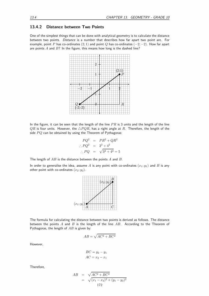
13.4 CHAPTER 13. GEOMETRY - GRADE 10
13.4.2 Distance between Two Points
One of the simplest things that can be done with analytical geometry is to calculate the distancebetween two points. Distance is a number that describes how far apart two point are. Forexample, point P has co-ordinates (2; 1) and point Q has co-ordinates (−2;−2). How far apartare points A and B? In the figure, this means how long is the dashed line?
1 2−1−2
1
2
−1
−2
b
b
(2;1)P
(-2;-2)Q R
In the figure, it can be seen that the length of the line PR is 3 units and the length of the lineQR is four units. However, the △PQR, has a right angle at R. Therefore, the length of theside PQ can be obtained by using the Theorem of Pythagoras:
PQ2 = PR2 + QR2
∴ PQ2 = 32 + 42
∴ PQ =√
32 + 42 = 5
The length of AB is the distance between the points A and B.
In order to generalise the idea, assume A is any point with co-ordinates (x1; y1) and B is anyother point with co-ordinates (x2; y2).
b
b
(x1; y1)
(x2; y2)
A
B
C
The formula for calculating the distance between two points is derived as follows. The distancebetween the points A and B is the length of the line AB. According to the Theorem ofPythagoras, the length of AB is given by:
AB =√
AC2 + BC2
However,
BC = y2 − y1
AC = x2 − x1
Therefore,
AB =√
AC2 + BC2
=√
(x1 − x2)2 + (y1 − y2)2
172

CHAPTER 13. GEOMETRY - GRADE 10 13.4
Therefore, for any two points, (x1; y1) and (x2; y2), the formula is:
Distance =√
(x1 − x2)2 + (y1 − y2)2
Using the formula, distance between the points P and Q with co-ordinates (2;1) and (-2;-2) isthen found as follows. Let the co-ordinates of point P be (x1; y1) and the co-ordinates of pointQ be (x2; y2). Then the distance is:
Distance =√
(x1 − x2)2 + (y1 − y2)2
=√
(2 − (−2))2 + (1 − (−2))2
=√
(2 + 2)2 + (1 + 2)2
=√
16 + 9
=√
25
= 5
13.4.3 Calculation of the Gradient of a Line
The gradient of a line describes how steep the line is. In the figure, line PT is the steepest. LinePS is less steep than PT but is steeper than PR, and line PR is steeper than PQ.
P
QR
ST
The gradient of a line is defined as the ratio of the vertical distance to the horizontal distance.This can be understood by looking at the line as the hypotenuse of a right-angled triangle. Thenthe gradient is the ratio of the length of the vertical side of the triangle to the horizontal side ofthe triangle. Consider a line between a point A with co-ordinates (x1; y1) and a point B withco-ordinates (x2; y2).
b
b
(x1; y1)
(x2; y2)
A
B
C
Gradient = y2−y1
x2−x1
For example the gradient of the line between the points P and Q, with co-ordinates (2;1) and(-2;-2) (Figure 13.4.2) is:
173

13.4 CHAPTER 13. GEOMETRY - GRADE 10
Gradient =y2 − y1
x2 − x1
=−2 − 1
−2 − 2
=−3
−4
=3
4
13.4.4 Midpoint of a Line
Sometimes, knowing the co-ordinates of the middle point or midpoint of a line is useful. Forexample, what is the midpoint of the line between point P with co-ordinates (2; 1) and point Qwith co-ordinates (−2;−2).
The co-ordinates of the midpoint of any line between any two points A and B with co-ordinates(x1; y1) and (x2; y2), is generally calculated as follows. Let the midpoint of AB be at point Swith co-ordinates (X ; Y ). The aim is to calculate X and Y in terms of (x1; y1) and (x2; y2).
b
b
b
(x1; y1)
(x2; y2)
(X ; Y )
A
B
S
X =x1 + x2
2
Y =y1 + y2
2
∴ S
(
x1 + x2
2;y1 + y2
2
)
Then the co-ordinates of the midpoint (S) of the line between point P with co-ordinates (2; 1)and point Q with co-ordinates (−2;−2) is:
X =x1 + x2
2
=−2 + 2
2= 0
Y =y1 + y2
2
=−2 + 1
2
= −1
2
∴ S(0;−1
2)
It can be confirmed that the distance from the each end point to the midpoint is equal. Theco-ordinate of the midpoint S is (0;−0,5).
174

CHAPTER 13. GEOMETRY - GRADE 10 13.4
PS =√
(x1 − x2)2 + (y1 − y2)2
=√
(0 − 2)2 + (−0.5 − 1)2
=√
(−2)2 + (−1.5)2
=√
4 + 2.25
=√
6.25
and
QS =√
(x1 − x2)2 + (y1 − y2)2
=√
(0 − (−2))2 + (−0.5 − (−2))2
=√
(0 + 2))2 + (−0.5 + 2))2
=√
(2))2 + (−1.5))2
=√
4 + 2.25
=√
6.25
It can be seen that PS = QS as expected.
1 2−1−2
1
2
−1
−2
b
b
b
(2;1)P
Q(-2;-2)
midpointS
Exercise: Co-ordinate Geometry
1. In the diagram given the vertices of a quadrilateral are F(2;0), G(1;5), H(3;7)
175

13.4 CHAPTER 13. GEOMETRY - GRADE 10
and I(7;2).
-1 0 1 2 3 4 5 6 7
-1
0
1
2
3
4
5
6
7
F(2;0)
G(1;5)
H(3;7)
I(7;2)
a) What are the lengths of the opposite sides of FGHI?
b) Are the opposite sides of FGHI parallel?
c) Do the diagonals of FGHI bisect each other?
d) Can you state what type of quadrilateral FGHI is? Give reasons for youranswer.
2. A quadrialteral ABCD with vertices A(3;2), B(1;7), C(4;5) and D(1;3) is given.
a) Draw the qaudrilateral.
b) Find the lengths of the sides of the quadrilateral.
3. S(1;4), T(-1;2), U(0;-1) and V(4;-1) are the vertices of a pentagon.
a) Are two of the sides of this pentagon parallel? If yes, find them.
b) Are two of the sides of this pentagon of equal length? If yes, find them.
4. ABCD is a quadrilateral with verticies A(0;3), B(4;3), C(5;-1) and D(-1;-1).
a) Show that:
(i) AD = BC
(ii) AB ‖ DC
b) What name would you give to ABCD?
c) Show that the diagonals AC and BD do not bisect each other.
5. P, Q, R and S are the points (-2;0), (2;3), (5;3), (-3;-3) respectively.
a) Show that:
(i) SR = 2PQ
(ii) SR ‖ PQ
b) Calculate:
(i) PS
(ii) QR
c) What kind of a quadrilateral is PQRS? Give reasons for your answers.
6. EFGH is a parallelogram with verticies E(-1;2), F(-2;-1) and G(2;0). Find theco-ordinates of H by using the fact that the diagonals of a parallelogram bisecteach other.
176

CHAPTER 13. GEOMETRY - GRADE 10 13.5
13.5 Transformations
In this section you will learn about how the co-ordinates of a point change when the point ismoved horizontally and vertically on the Cartesian plane. You will also learn about what happensto the co-ordinates of a point when it is reflected on the x-axis, y-axis and the line y = x.
13.5.1 Translation of a Point
When something is moved in a straight line, we say that it is translated. What happens to theco-ordinates of a point that is translated horizontally or vertically?
Activity :: Discussion : Translation of a Point Vertically
Complete the table, by filling in the co-ordinates of the points shown in the figure.
1 2
1
2
3
−1
−2
−3
b
b
b
b
b
b
b
C
B
A
D
E
F
G
Point x co-ordinate y co-ordinate
ABCDEFG
What do you notice about the x co-ordinates? What do you notice about they co-ordinates?What would happen to the co-ordinates ofpoint A, if it was moved to the position ofpoint G?
When a point is moved vertically up or down on the Cartesian plane, the x co-ordinate of thepoint remains the same, but the y co-ordinate changes by the amount that the point was movedup or down.
For example, in Figure 13.3 Point A is moved 4 units upwards to the position marked by G.The new x co-ordinate of point A is the same (x=1), but the new y co-ordinate is shifted inthe positive y direction 4 units and becomes y=-2+4=2. The new co-ordinates of point A aretherefore G(1;2). Similarly, for point B that is moved downwards by 5 units, the x co-ordinateis the same (x = −2,5), but the y co-ordinate is shifted in the negative y-direction by 5 units.The new y co-ordinate is therefore y=2,5 -5=-2,5.
Important: If a point is shifted upwards, the new y co-ordinate is given by adding the shiftto the old y co-ordinate. If a point is shifted downwards, the new y co-ordinate is given bysubtracting the shift from the old y co-ordinate.
Activity :: Discussion : Translation of a Point HorizontallyComplete the table, by filling in the co-ordinates of the points shown in the figure.
177

13.5 CHAPTER 13. GEOMETRY - GRADE 10
1 2−1−2
1
2
3
−1
−2
−3
b
b
b
b
A (1;-2)
G
B (-2.5;2.5)
H
4units5
units
Figure 13.3: Point A is moved 4 units upwards to the position marked by G. Point B is 5 unitsdownwards to the position marked by H.
1 2 3−1−2−3
1
2bbb b b b bCBA D E F G
Point x co-ordinate y co-ordinate
ABCDEFG
What do you notice about the x co-ordinates? What do you notice about the yco-ordinates?
What would happen to the co-ordinates of point A, if it was moved to the positionof point G?
When a point is moved horizontally left or right on the Cartesian plane, the y co-ordinate of thepoint remains the same, but the x co-ordinate changes by the amount that the point was movedleft or right.
For example, in Figure 13.4 Point A is moved 4 units right to the position marked by G. Thenew y co-ordinate of point A is the same (y=1), but the new x co-ordinate is shifted in thepositive x direction 4 units and becomes x=-2+4=2. The new co-ordinate of point A at G istherefore (2;1). Similarly, for point B that is moved left by 5 units, the y co-ordinate is the same(y = −2,5), but the x co-ordinate is shifted in the negative x-direction by 5 units. The newx co-ordinate is therefore x=2,5 -5=-2,5. The new co-ordinates of point B at H is therefore(-2,5;1).
178

CHAPTER 13. GEOMETRY - GRADE 10 13.5
1 2 3−1−2−3
1
2
−1
−2
b
b
b
b
A (-2;1) G
B (2.5;-2.5)H
4 units
5 units
Figure 13.4: Point A is moved 4 units to the right to the position marked by G. Point B is 5units to the left to the position marked by H.
Important: If a point is shifted to the right, the new x co-ordinate is given by adding theshift to the old x co-ordinate. If a point is shifted to the left, the new x co-ordinate is givenby subtracting the shift from the old x co-ordinate.
13.5.2 Reflection of a Point
When you stand in front of a mirror your reflection is located the same distance (d) behind themirror as you are standing in front of the mirror.
mirroryou your reflection
d d
We can apply the same idea to a point that is reflected on the x-axis, the y-axis and the liney = x.
Reflection on the x-axis
If a point is reflected on the x-axis, then the reflection must be the same distance below thex-axis as the point is above the x-axis and vice-versa.
Important: When a point is reflected about the x-axis, only the y co-ordinate of the pointchanges.
179

13.5 CHAPTER 13. GEOMETRY - GRADE 10
1 2 3−1−2−3
1
2
−1
−2
b
b
bc
bc
A (-1;2)
B (2;-1)
A’ (-1;-2)
B’ (2;1)
Figure 13.5: Points A and B are reflected on the x-axis. The original points are shown with •and the reflected points are shown with ◦.
Worked Example 53: Reflection on the x-axis
Question: Find the co-ordinates of the reflection of the point P, if P is reflected onthe x-axis. The co-ordinates of P are (5;10).AnswerStep 1 : Determine what is given and what is requiredWe are given the point P with co-ordinates (5;10) and need to find the co-ordinatesof the point if it is reflected on the x-axis.Step 2 : Determine how to approach the problemThe point P is above the x-axis, therefore its reflection will be the same distancebelow the x-axis as the point P is above the x-axis. Therefore, y=-10.For a reflection on the x-axis, the x co-ordinate remains unchanged. Therefore,x=5.Step 3 : Write the final answerThe co-ordinates of the reflected point are (5;-10).
Reflection on the y-axis
If a point is reflected on the y-axis, then the reflection must be the same distance to the left ofthe y-axis as the point is to the right of the y-axis and vice-versa.
Important: When a point is reflected on the y-axis, only the x co-ordinate of the pointchanges. The y co-ordinate remains unchanged.
Worked Example 54: Reflection on the y-axis
Question: Find the co-ordinates of the reflection of the point Q, if Q is reflectedon the y-axis. The co-ordinates of Q are (15;5).AnswerStep 1 : Determine what is given and what is required
180

CHAPTER 13. GEOMETRY - GRADE 10 13.5
1 2 3−1−2−3
1
2
−1
−2
b
b
bc
bc
A (2;-1)
B (-1;2)
A’ (-2;-1)
B’ (1;2)
Figure 13.6: Points A and B are reflected on the y-axis. The original points are shown with •and the reflected points are shown with ◦.
We are given the point Q with co-ordinates (15;5) and need to find the co-ordinatesof the point if it is reflected on the y-axis.Step 2 : Determine how to approach the problemThe point Q is to the right of the y-axis, therefore its reflection will be the samedistance to the left of the y-axis as the point Q is to the right of the y-axis. Therefore,x=-15.For a reflection on the y-axis, the y co-ordinate remains unchanged. Therefore, y=5.Step 3 : Write the final answerThe co-ordinates of the reflected point are (-15;5).
Reflection on the line y = x
The final type of reflection you will learn about is the reflection of a point on the line y = x.
Activity :: Casestudy : Reflection of a point on the line y = x
1 2 3−1−2−3
1
2
3
−1
−2
−3
b
b
b
b
bc
bc
A (2;1)
B (-1 12 ;-2)
C (-1;1)
D (2;-3)
A’ (1;2)
B’ (-2;-1 12 )
Study the information given and complete the following table:
181

13.5 CHAPTER 13. GEOMETRY - GRADE 10
Point Reflection
A (2;1) (1;2)
B (-1 12 ;-2) (-2;-1 1
2 )C (-1;1)D (2;-3)
What can you deduce about the co-ordinates of points that are reflected aboutthe line y = x?
The x and y co-ordinates of points that are reflected on the line y = x are swapped around, orinterchanged. This means that the x co-ordinate of the original point becomes the y co-ordinateof the reflected point and the y co-ordinate of the original point becomes the x co-ordinate ofthe reflected point.
1 2 3−1−2−3
1
2
3
−1
−2
−3
b
b
bc
bc
A (3;1)
B (-2;-1)
A’ (1;3)
B’ (-1;-2)
Figure 13.7: Points A and B are reflected on the line y = x. The original points are shown with• and the reflected points are shown with ◦.
Important: The x and y co-ordinates of points that are reflected on the line y = x areinterchanged.
Worked Example 55: Reflection on the line y = x
Question: Find the co-ordinates of the reflection of the point R, if R is reflected onthe line y = x. The co-ordinates of R are (-5;5).AnswerStep 1 : Determine what is given and what is requiredWe are given the point R with co-ordinates (-5;5) and need to find the co-ordinatesof the point if it is reflected on the line y = x.Step 2 : Determine how to approach the problemThe x co-ordinate of the reflected point is the y co-ordinate of the original point.Therefore, x=5.The y co-ordinate of the reflected point is the x co-ordinate of the original point.Therefore, y=-5.Step 3 : Write the final answerThe co-ordinates of the reflected point are (5;-5).
182

CHAPTER 13. GEOMETRY - GRADE 10 13.5
Rules of TranslationA quick way to write a translation is to use a ’rule of translation’. For example (x; y) →(x + a; y + b) means translate point (x;y) by moving a units horizontally and b units vertically.So if we translate (1;2) by the rule (x; y) → (x + 3; y − 1) it becomes (4;1). We have moved 3units right and 1 unit down.Translating a RegionTo translate a region, we translate each point in the region.ExampleRegion A has been translated to region B by the rule: (x; y) → (x + 4; y + 2)
AA
B
(-3;1) (-2;1)
(-3;0) (-2;0)
(1;3) (2;3)
(2;2)(1;2)
Activity :: Discussion : Rules of TransformationsWork with a friend and decide which item from column 1 matches each descrip-
tion in column 2.
Column 1 Column 2
(x; y) → (x; y − 3) a reflection on x-y line
(x; y) → (x − 3; y) a reflection on the x axis
(x; y) → (x;−y) a shift of 3 units left
(x; y) → (−x; y) a shift of 3 units down
(x; y) → (y; x) a reflection on the y-axis
Exercise: Transformations
1. Find the co-ordinates of each of the points ( S - Z) if they are reflected aboutthe given lines:
a) y-axis (x=0)
183

13.5 CHAPTER 13. GEOMETRY - GRADE 10
b) x-axis (y=0)
c) y=-x
d) y=x
-6 -5 -4 -3 -2 -1 0 1 2 3 4 5 6
-6
-5
-4
-3
-2
-1
0
1
2
3
4
5
6
b
b
b
b
b
b
b
b
S
T
U
V
W
X
Y
Z
x-axis
y-axis
2. Write down the rule used for each of the following reflections:
a) Z(7;3), Z’(3;7)
b) Y(-1;-8), Y’(1;-8)
c) X(5;9), X’(-5;9)
d) W(4;6), W’(4;6)
e) V(−37 ; 53 ), V’(5
3 ;−37 )
3. a) Reflect the given points using the rules that are given.
b) Identify the line of reflection in each case (some may not exist):
(i) H(-4;3); (x;y)→ (-x;y)
(ii) H(-4;3); (x;y) → (-y;-x)
(iii) H(-4;3); (x;y) → (y;x)
(iv) H(-4;3); (x;y) → (-x;-y)
(v) H(-4;3); (x;y) → (x;-y)
4. 0 1 2 3 4 5 60
1
2
3
4
5
6
(5;1)
Using squared paper, copy the diagram given. Let -10≤x≤10, -10≤y≤10.
184

CHAPTER 13. GEOMETRY - GRADE 10 13.6
i) Identify the transformation.
ii) Draw the image of the figure according the rules given.
a) (x; y) → (−x; y)
b) (x; y) → (y; x)
c) (x; y) → (x; y − 3)
d) (x; y) → (x + 5; y)
e) (x; y) → (x;−y)
Activity :: Investigation : Calculation of Volume, Surface Area and scalefactors of objects
1. Look around the house or school and find a can or a tin of any kind (e.g. beans,soup, cooldrink, paint etc.)
2. Measure the height of the tin and the diameter of its top or bottom.
3. Write down the values you measured on the diagram below:
side top bottom
4. Using your measurements, calculate the following (in cm2, rounded off to 2decimal places):
(a) the area of the side of the tin (i.e. the rectangle)
(b) the area of the top and bottom of the tin (i.e. the circles)
(c) the total surface area of the tin
5. If the tin metal costs 0,17 cents/cm2, how much does it cost to make the tin?
6. Find the volume of your tin (in cm3, rounded off to 2 decimal places).
7. What is the volume of the tin given on its label?
8. Compare the volume you calculated with the value given on the label. Howmuch air is contained in the tin when it contains the product (i.e. cooldrink,soup etc.)
9. Why do you think space is left for air in the tin?
10. If you wanted to double the volume of the tin, but keep the radius the same,by how much would you need to increase the height?
11. If the height of the tin is kept the same, but now the radius is doubled, by whatscale factor will the:
(a) area of the side surface of the tin increase?
(b) area of the bottom/top of the tin increase?
13.6 End of Chapter Exercises
1. Write a rule that will give the following transformations of DEFG to D’E’F’G in each case.
185

13.6 CHAPTER 13. GEOMETRY - GRADE 10
a)
-6 -5 -4 -3 -2 -1 0 1 2 3 4 5 6
-6
-5
-4
-3
-2
-1
0
1
2
3
4
5
D
F
G
D’ E’
F’
G’
E
b)
-6 -5 -4 -3 -2 -1 0 1 2 3 4 5 6
-3
-2
-1
0
1
2
3
4
5
D
E
F
G
D’
E’
F’
G’
2. Using the rules given, identify the type of transformation and draw the image of the shapes.
a) (x;y)→(x+3;y-3)
-6 -5 -4 -3 -2 -1 0 1 2 3 4 5 6
-1
0
1
2
3
4
5
6
b) (x;y)→(x-4;y)
-6 -5 -4 -3 -2 -1 0 1 2 3 4 5 6
-1
0
1
2
3
4
5
6
c) (x;y)→(y;x)
-6 -5 -4 -3 -2 -1 0 1 2 3 4 5 6
-6
-5
-4
-3
-2
-1
0
1
186

CHAPTER 13. GEOMETRY - GRADE 10 13.6
d) (x;y)→(-x;-y)
-6 -5 -4 -3 -2 -1 0 1 2 3 4 5 6
-6
-5
-4
-3
-2
-1
0
1
187

13.6 CHAPTER 13. GEOMETRY - GRADE 10
188

Chapter 14
Trigonometry - Grade 10
14.1 Introduction
In geometry we learn about how the sides of polygons relate to the angles in the polygons,but we have not learned how to calculate an angle if we only know the lengths of the sides.Trigonometry (pronounced: trig-oh-nom-eh-tree) deals with the relationship between the anglesand the sides of a right-angled triangle. We will learn about trigonometric functions, which formthe basis of trigonometry.
Activity :: Investigation : History of TrigonometryWork in pairs or groups and investigate the history of the foundation of trigonom-
etry. Describe the various stages of development and how the following cultures usedtrigonometry to improve their lives.
The works of the following people or cultures can be investigated:
1. Cultures
(a) Ancient Egyptians
(b) Mesopotamians
(c) Ancient Indians of the Indus Valley
2. People
(a) Lagadha (circa 1350-1200 BC)
(b) Hipparchus (circa 150 BC)
(c) Ptolemy (circa 100)
(d) Aryabhata (circa 499)
(e) Omar Khayyam (1048-1131)
(f) Bhaskara (circa 1150)
(g) Nasir al-Din (13th century)
(h) al-Kashi and Ulugh Beg (14th century)
(i) Bartholemaeus Pitiscus (1595)
Interesting
Fact
teresting
FactYou should be familiar with the idea of measuring angles from geometry buthave you ever stopped to think why there are 360 degrees in a circle? Thereason is purely historical. There are 360 degrees in a circle because the ancient
189

14.2 CHAPTER 14. TRIGONOMETRY - GRADE 10
Babylonians had a number system with base 60. A base is the number you countup to before you get an extra digit. The number system that we use everyday iscalled the decimal system (the base is 10), but computers use the binary system(the base is 2). 360 = 6 × 60 so for them it made sense to have 360 degrees in acircle.
14.2 Where Trigonometry is Used
There are many applications of trigonometry. Of particular value is the technique of triangulation,which is used in astronomy to measure the distance to nearby stars, in geography to measuredistances between landmarks, and in satellite navigation systems. GPSs (global positioning sys-tems) would not be possible without trigonometry. Other fields which make use of trigonometryinclude astronomy (and hence navigation, on the oceans, in aircraft, and in space), music theory,acoustics, optics, analysis of financial markets, electronics, probability theory, statistics, biology,medical imaging (CAT scans and ultrasound), pharmacy, chemistry, number theory (and hencecryptology), seismology, meteorology, oceanography, many physical sciences, land surveying andgeodesy, architecture, phonetics, economics, electrical engineering, mechanical engineering, civilengineering, computer graphics, cartography, crystallography and game development.
Activity :: Discussion : Uses of TrigonometrySelect one of the uses of trigonometry from the list given and write a 1-page
report describing how trigonometry is used in your chosen field.
14.3 Similarity of Triangles
If △ABC is similar to △DEF , then this is written as:
△ABC ∼ △DEF
b
A
b B
bC
b
D
b E
bF
Then, it is possible to deduce proportionalities between corresponding sides of the two triangles,such as the following:
ABBC= DE
EF
ABAC= DE
DF
190

CHAPTER 14. TRIGONOMETRY - GRADE 10 14.4
ACBC=DF
EF
ABDE= BC
EF= AC
DF
The most important fact about similar triangles ABC and DEF is that the
angle at vertex A is equal to the angle at vertex D, the angle at B is equal to the angle at E,and the angle at C is equal to the angle at F.
∠A = ∠D
∠B = ∠E
∠C = ∠F
Activity :: Investigation : Ratios of Similar TrianglesIn your exercise book, draw three similar triangles of different sizes, but each
with A = 30◦; B = 90◦ and C = 60◦. Measure angles and lengths very accuratelyin order to fill in the table below (round answers to one decimal place).
C C′ C′′B B′ B′′
A
A′A′′
30
60 60 60
30
30
Dividing lengths of sides (Ratios)ABBC
= ABAC
= CBAC
=A′B′
B′C′= A′B′
A′C′= C′B′
A′C′=
A′′B′′
B′′C′′= A′′B′′
A′′C′′= C′′B′′
A′′C′′=
What observations can you make about the ratios of the sides?These equal ratios are used to define the trigonometric functions.
Note: In algebra, we often use the letter x for our unknown variable (althoughwe can use any other letter too, such as a, b, k, etc). In trigonometry, we often usethe Greek symbol θ for an unknown angle (we also use α , β , γ etc).
14.4 Definition of the Trigonometric Functions
We are familiar with a function of the form f(x) where f is the function and x is the argument.Examples are:
f(x) = 2x (exponential function)
g(x) = x + 2 (linear function)
h(x) = 2x2 (parabolic function)
The basis of trigonometry are the trigonometric functions. There are three basic trigonometricfunctions:
1. sine
191

14.4 CHAPTER 14. TRIGONOMETRY - GRADE 10
2. cosine
3. tangent
These are abbreviated to:
1. sin
2. cos
3. tan
These functions are defined from a right-angled triangle.
Consider a right-angled triangle.
b
A
b
B
b
Cθ
opposite
hypotenuse
adjacent
In the right-angled triangle, we refer to the lengths of the three sides according to how they areplaced in relation to the angle θ. The side opposite to θ is labelled opposite, the side next to θis labelled adjacent and the side opposite the right-angle is labelled the hypotenuse.
We define:
sin θ =opposite
hypotenuse
cos θ =adjacent
hypotenuse
tan θ =opposite
adjacent
These functions relate the lengths of the sides of a triangle to its interior angles.
One way of remembering the definitions is to use the following mnemonic that is perhaps easierto remember:
Silly Old Hens Sin = OppositeHypotenuse
Cackle And Howl Cos = AdjacentHypotenuse
Till Old Age Tan = OppositeAdjacent
Important: The definitions of opposite, adjacent and hypotenuse only make sense whenyou are working with right-angled triangles! Always check to make sure your triangle hasa right-angle before you use them, otherwise you will get the wrong answer. We will findways of using our knowledge of right-angled triangles to deal with the trigonometry of nonright-angled triangles in Grade 11.
Activity :: Investigation : Definitions of Trigonometric Functions
192

CHAPTER 14. TRIGONOMETRY - GRADE 10 14.4
1. In each of the following triangles, state whether a, b and c are the hypotenuse,opposite or adjacent sides of the triangle.
b
θ
θ
θ
θ
θ
θ
a
b
ca
c
b
ab
c
a
bc
a
b
c
ab
c
2. Complete each of the following, the first has been done for youA
BC
a) sin A =opposite
hypotenuse=
CB
AC
b) cos A =
c) tan A =
d) sin C =
e) cos C =
f) tan C =
3. Complete each of the following:
2
60o
30o
√2
sin 60 =
cos 30 =
tan 60 =
1
45o
45o
√2
1 sin 45 =
cos 45 =
tan 45 =
For most angles θ, it is very difficult to calculate the values of sin θ, cos θ and tan θ. One usuallyneeds to use a calculator to do so. However, we saw in the above Activity that we could workthese values out for some special angles. Some of these angles are listed in the table below,along with the values of the trigonometric functions at these angles.
0◦ 30◦ 45◦ 60◦ 90◦ 180◦
cos θ 1√
32
1√2
12 0 −1
sin θ 0 12
1√2
√3
2 1 0
tan θ 0 1√3
1√
3 − 0
These values are useful when asked to solve a problem involving trig functions without using acalculator.
Worked Example 56: Finding Lengths
Question: Find the length of x in the following triangle.
193

14.4 CHAPTER 14. TRIGONOMETRY - GRADE 10
100m
50◦
x
AnswerStep 1 : Identify the trig identity that you needIn this case you have an angle (50◦), the opposite side and the hypotenuse.So you should use sin
sin 50◦ =x
100
Step 2 : Rearrange the question to solve for x
⇒ x = 100 × sin 50◦
Step 3 : Use your calculator to find the answer
Use the sin button on your calculator
⇒ x = 76.6m
Worked Example 57: Finding Angles
Question: Find the value of θ in the following triangle.
100m
50m
θ
AnswerStep 1 : Identify the trig identity that you needIn this case you have the opposite side and the hypotenuse to the angle θ.So you should use tan
tan θ =50
100
Step 2 : Calculate the fraction as a decimal number
⇒ tan θ = 0.5
Step 3 : Use your calculator to find the angleSince you are finding the angle,
use tan−1 on your calculatorDon’t forget to set your calculator to ‘deg’ mode!
⇒ θ = 26.6◦
194

CHAPTER 14. TRIGONOMETRY - GRADE 10 14.5
Exercise: Finding LengthsFind the length of the sides marked with letters. Give answers correct to 2
decimal places.
a) b)
c) d)
37◦
62
a
23◦
21
b
55◦19
c 33
49◦
d
e) f)
g) h)
e
17◦
12
22◦f
31
32
23◦
g
h
30◦
20
14.5 Simple Applications of Trigonometric Functions
Trigonometry was probably invented in ancient civilisations to solve practical problems involvingconstructing buildings and navigating their ships by the stars. In this section we will show howtrigonometry can be used to solve some other practical problems.
14.5.1 Height and Depth
One simple task is to find the height of a building by using trigonometry. We could just use atape measure lowered from the roof but this is impractical (and dangerous) for tall buildings. Itis much more sensible to measure a distance along the ground and use trigonometry to find theheight of the building.
Figure 14.1 shows a building whose height we do not know. We have walked 100 m away fromthe building and measured the angle up to the top. This angle is found to be 38,7◦. We call
195

14.5 CHAPTER 14. TRIGONOMETRY - GRADE 10
100m
38.7◦
Figure 14.1: Determining the height of a building using trigonometry.
this angle the angle of elevation. As you can see from Figure 14.1, we now have a right-angledtriangle. As we know the length of one side and an angle, we can calculate the height of thetriangle, which is the height of the building we are trying to find.
If we examine the figure, we see that we have the opposite and the adjacent of the angle ofelevation and we can write:
tan 38,7◦ =opposite
adjacent
=height
100 m⇒ height = 100 m× tan 38,7◦
= 80 m
Worked Example 58: Height of a tower
Question: A block of flats is 100m away from a cellphone tower. Someone at Ameasures the angle of elevation to the top of the tower E to be 62◦, and the angleof depression to the bottom of the tower C to be 34◦. What is the height of thecellphone tower correct to 1 decimal place?
b
A
B
C
D
E
62◦
34◦
100m
AnswerStep 1 : Identify a strategyTo find the height of the tower, all we have to do is find the length of CD and DE.We see that △ACD and △AED are both right-angled. For each of the triangles,we have an angle and we have the length AD. Thus we can calculate the sides ofthe triangles.Step 2 : Calculate CD
196

CHAPTER 14. TRIGONOMETRY - GRADE 10 14.5
tan(CAD) =CD
AD
=⇒ CD = AD × tan(CAD)
= 100 × tan 34◦
Use your calculator to find that tan 34◦ = 0,6745. Using this, we find that CD =67,45mStep 3 : Calculate DE
tan(DAE) =DE
AD
=⇒ DE = AD × tan(DAE)
= 100 × tan 62◦
= 188,07 m
Step 4 : Combine the previous answersWe have that the height of the tower CE = CD + DE = 67,45 m + 188,07 m =255.5 m.
14.5.2 Maps and Plans
Maps and plans are usually scale drawings. This means that they are an exact copy of the realthing, but are usually smaller. So, only lengths are changed, but all angles are the same. Wecan use this idea to make use of maps and plans by adding information from the real world.
Worked Example 59: Scale Drawing
Question: A ship approaching Cape Town Harbour reaches point A on the map,due South of Pretoria and due East of Cape Town. If the distance from Cape Townto Pretoria is 1000km, use trigonometry to find out how far East the ship is to CapeTown, and hence find the scale of the map.
b
b b
Cape Town
Pretoria
A
197

14.5 CHAPTER 14. TRIGONOMETRY - GRADE 10
AnswerStep 1 : Identify what happens in the questionWe already know the distance between Cape Town and A in blocks from the givenmap (it is 5 blocks). Thus if we work out how many kilometers this same distanceis, we can calculate how many kilometers each block represents, and thus we havethe scale of the map.Step 2 : Identify given informationLet us denote Cape Town with C and Pretoria with P . We can see that triangle APCis a right-angled triangle. Furthermore, we see that the distance AC and distanceAP are both 5 blocks. Thus it is an isoceles triangle, and so ACP = APC = 45◦.Step 3 : Carry out the calculation
CA = CP × cos(ACP )
= 1000× cos(45◦)
= 1000√2
km
To work out the scale, we see that
5 blocks = 1000√2
km
=⇒ 1 block = 200√2
km
Worked Example 60: Building plan
Question: Mr Nkosi has a garage at his house, and he decides that he wants toadd a corrugated iron roof to the side of the garage. The garage is 4m high, andhis sheet for the roof is 5m long. If he wants the roof to be at an angle of 5◦, howhigh must he build the wall BD, which is holding up the roof? Give the answer to2 decimal places.
4m
5m
B
A
5◦
Garage
RoofC
Wall
b
b
b
D
AnswerStep 1 : Set out strategyWe see that the triangle ABC is a right-angled triangle. As we have one side andan angle of this triangle, we can calculate AC. The height of the wall is then theheight of the garage minus AC.Step 2 : Execute strategyIf BC=5m, and angle ABC = 5◦, then
AC = BC × sin(ABC)
= 5 × sin 5◦
= 5 × 0,0871
= 0.4358 m
Thus we have that the height of the wall BD = 5 m − 0.4358 m = 4.56 m.
198

CHAPTER 14. TRIGONOMETRY - GRADE 10 14.6
Exercise: Applications of Trigonometric Functions
1. A boy flying a kite is standing 30 m from a point directly under the kite. If thestring to the kite is 50 m. long, find the angle of elevation of the kite.
2. What is the angle of elevation of the sun when a tree 7,15 m tall casts a shadow10,1 m long?
14.6 Graphs of Trigonometric Functions
This section describes the graphs of trigonometric functions.
14.6.1 Graph of sin θ
Activity :: Graph of sin θ : Complete the following table, using yourcalculator to calculate the values. Then plot the values with sin θ on they-axis and θ on the x-axis. Round answers to 1 decimal place.
θ 0◦ 30◦ 60◦ 90◦ 120◦ 150◦
sin θθ 180◦ 210◦ 240◦ 270◦ 300◦ 330◦ 360◦
sin θ
30 60 90 120 150 180 210 240 270 300 330 3600
1
−1
Let us look back at our values for sin θ
θ 0◦ 30◦ 45◦ 60◦ 90◦ 180◦
sin θ 0 12
1√2
√3
2 1 0
As you can see, the function sin θ has a value of 0 at θ = 0◦. Its value then smoothly increasesuntil θ = 90◦ when its value is 1. We then know that it later decreases to 0 when θ = 180◦.Putting all this together we can start to picture the full extent of the sine graph. The sine graphis shown in Figure 14.2. Notice the wave shape, with each wave having a length of 360◦. Wesay the graph has a period of 360◦. The height of the wave above (or below) the x-axis is calledthe waves’ amplitude. Thus the maximum amplitude of the sine-wave is 1, and its minimumamplitude is -1.
199

14.6 CHAPTER 14. TRIGONOMETRY - GRADE 10
180 360−180−360
1
−1
Figure 14.2: The graph of sin θ.
90 180 270−90−180−270
1
2
3
4
5
−1
Figure 14.3: Graph of f(θ) = 2 sin θ + 3
14.6.2 Functions of the form y = a sin(x) + q
In the equation, y = a sin(x) + q, a and q are constants and have different effects on the graphof the function. The general shape of the graph of functions of this form is shown in Figure 14.3for the function f(θ) = 2 sin θ + 3.
Activity :: Functions of the Form y = a sin(θ) + q :
1. On the same set of axes, plot the following graphs:
(a) a(θ) = sin θ − 2
(b) b(θ) = sin θ − 1
(c) c(θ) = sin θ
(d) d(θ) = sin θ + 1
(e) e(θ) = sin θ + 2
Use your results to deduce the effect of q.
2. On the same set of axes, plot the following graphs:
(a) f(θ) = −2 · sin θ
(b) g(θ) = −1 · sin θ
(c) h(θ) = 0 · sin θ
200

CHAPTER 14. TRIGONOMETRY - GRADE 10 14.6
(d) j(θ) = 1 · sin θ
(e) k(θ) = 2 · sin θ
Use your results to deduce the effect of a.
You should have found that the value of a affects the height of the peaks of the graph. As themagnitude of a increases, the peaks get higher. As it decreases, the peaks get lower.q is called the vertical shift. If q = 2, then the whole sine graph shifts up 2 units. If q = −1,the whole sine graph shifts down 1 unit.
These different properties are summarised in Table 14.1.
Table 14.1: Table summarising general shapes and positions of graphs of functions of the formy = a sin(x) + q.
a > 0 a < 0
q > 0
q < 0
Domain and Range
For f(θ) = a sin(θ) + q, the domain is {θ : θ ∈ R} because there is no value of θ ∈ R for whichf(θ) is undefined.
The range of f(θ) = a sin θ + q depends on whether the value for a is positive or negative. Wewill consider these two cases separately.
If a > 0 we have:
-1 ≤ sin θ ≤ 1
-a ≤ a sin θ ≤ a (Multiplication by a positive number maintains the nature of the inequality)
-a+q ≤ a sin θ + q ≤ a + q
-a+q ≤ f(θ) ≤ a + qThis tells us that for all values of θ, f(θ) is always between −a + q anda + q. Therefore if a > 0, the range of f(θ) = a sin θ + q is {f(θ) : f(θ) ∈ [−a + q,a + q]}.Similarly, it can be shown that if a < 0, the range of f(θ) = a sin θ + q is {f(θ) : f(θ) ∈[a + q, − a + q]}. This is left as an exercise.
Important: The easiest way to find the range is simply to look for the ”bottom” and the”top” of the graph.
201

14.6 CHAPTER 14. TRIGONOMETRY - GRADE 10
Intercepts
The y-intercept, yint, of f(θ) = a sin(x) + q is simply the value of f(θ) at θ = 0◦.
yint = f(0◦)
= a sin(0◦) + q
= a(0) + q
= q
14.6.3 Graph of cos θ
Activity :: Graph of cos θ : Complete the following table, using yourcalculator to calculate the values correct to 1 decimal place. Then plot thevalues with cos θ on the y-axis and θ on the x-axis.
θ 0◦ 30◦ 60◦ 90◦ 120◦ 150◦
cos θθ 180◦ 210◦ 240◦ 270◦ 300◦ 330◦ 360◦
cos θ
30 60 90 120 150 180 210 240 270 300 330 3600
1
−1
Let us look back at our values for cos θ
θ 0◦ 30◦ 45◦ 60◦ 90◦ 180◦
cos θ 1√
32
1√2
12 0 −1
If you look carefully, you will notice that the cosine of an angle θ is the same as the sine of theangle 90◦ − θ. Take for example,
cos 60◦ =1
2= sin 30◦ = sin (90◦ − 60◦)
This tells us that in order to create the cosine graph, all we need to do is to shift the sine graph90◦ to the left. The graph of cos θ is shown in figure 14.6. As the cosine graph is simply ashifted sine graph, it will have the same period and amplitude as the sine graph.
14.6.4 Functions of the form y = a cos(x) + q
In the equation, y = a cos(x) + q, a and q are constants and have different effects on the graphof the function. The general shape of the graph of functions of this form is shown in Figure 14.5for the function f(θ) = 2 cos θ + 3.
Activity :: Functions of the Form y = a cos(θ) + q :
1. On the same set of axes, plot the following graphs:
202

CHAPTER 14. TRIGONOMETRY - GRADE 10 14.6
180 360−180−360
1
−1
Figure 14.4: The graph of cos θ.
90 180 270−90−180−270
1
2
3
4
5
−1
Figure 14.5: Graph of f(θ) = 2 cos θ + 3
(a) a(θ) = cos θ − 2
(b) b(θ) = cos θ − 1
(c) c(θ) = cos θ
(d) d(θ) = cos θ + 1
(e) e(θ) = cos θ + 2
Use your results to deduce the effect of q.
2. On the same set of axes, plot the following graphs:
(a) f(θ) = −2 · cos θ
(b) g(θ) = −1 · cos θ
(c) h(θ) = 0 · cos θ
(d) j(θ) = 1 · cos θ
(e) k(θ) = 2 · cos θ
Use your results to deduce the effect of a.
You should have found that the value of a affects the amplitude of the cosine graph in the sameway it did for the sine graph.
You should have also found that the value of q shifts the cosine graph in the same way as it didthe sine graph.
These different properties are summarised in Table 14.2.
203

14.6 CHAPTER 14. TRIGONOMETRY - GRADE 10
Table 14.2: Table summarising general shapes and positions of graphs of functions of the formy = a cos(x) + q.
a > 0 a < 0
q > 0
q < 0
Domain and Range
For f(θ) = a cos(θ) + q, the domain is {θ : θ ∈ R} because there is no value of θ ∈ R for whichf(θ) is undefined.
It is easy to see that the range of f(θ) will be the same as the range of a sin(θ) + q. This isbecause the maximum and minimum values of a cos(θ) + q will be the same as the maximumand minimum values of a sin(θ) + q.
Intercepts
The y-intercept of f(θ) = a cos(x) + q is calculated in the same way as for sine.
yint = f(0◦)
= a cos(0◦) + q
= a(1) + q
= a + q
14.6.5 Comparison of Graphs of sin θ and cos θ
180 360−180−360
1
−1
90◦ shift
Figure 14.6: The graph of cos θ (solid-line) and the sine graph (dashed-line).
14.6.6 Graph of tan θ
Activity :: Graph of tan θ : Complete the following table, using yourcalculator to calculate the values correct to 1 decimal place. Then plot thevalues with tan θ on the y-axis and θ on the x-axis.
204

CHAPTER 14. TRIGONOMETRY - GRADE 10 14.6
θ 0◦ 30◦ 60◦ 90◦ 120◦ 150◦
tan θθ 180◦ 210◦ 240◦ 270◦ 300◦ 330◦ 360◦
tan θ
30 60 90 120 150 180 210 240 270 300 330 3600
1
−1
Let us look back at our values for tan θ
θ 0◦ 30◦ 45◦ 60◦ 90◦ 180◦
tan θ 0 1√3
1√
3 ∞ 0
Now that we have graphs for sin θ and cos θ, there is an easy way to visualise the tangent graph.Let us look back at our definitions of sin θ and cos θ for a right angled triangle.
sin θ
cos θ=
oppositehypotenuse
adjacenthypotenuse
=opposite
adjacent= tan θ
This is the first of an important set of equations called trigonometric identities. An identity isan equation, which holds true for any value, which is put into it. In this case we have shownthat
tan θ =sin θ
cos θ
for any value of θ.So we know that for values of θ for which sin θ = 0, we must also have tan θ = 0. Also, ifcos θ = 0 our value of tan θ is undefined as we cannot divide by 0. The graph is shown in Figure14.7. The dashed vertical lines are at the values of θ where tan θ is not defined.
180 360−180−360
2
4
−2
−4
Figure 14.7: The graph of tan θ.
14.6.7 Functions of the form y = a tan(x) + q
In the figure below is an example of a function of the form y = a tan(x) + q.
205

14.6 CHAPTER 14. TRIGONOMETRY - GRADE 10
180 360−180−360
5
10
−5
−10
Figure 14.8: The graph of 2 tan θ + 1.
Activity :: Functions of the Form y = a tan(θ) + q :
1. On the same set of axes, plot the following graphs:
(a) a(θ) = tan θ − 2
(b) b(θ) = tan θ − 1
(c) c(θ) = tan θ
(d) d(θ) = tan θ + 1
(e) e(θ) = tan θ + 2
Use your results to deduce the effect of q.
2. On the same set of axes, plot the following graphs:
(a) f(θ) = −2 · tan θ
(b) g(θ) = −1 · tan θ
(c) h(θ) = 0 · tan θ
(d) j(θ) = 1 · tan θ
(e) k(θ) = 2 · tan θ
Use your results to deduce the effect of a.
You should have found that the value of a affects the steepness of each of the branches. Youshould have also found that the value of q affects the vertical shift as for sin θ and cos θ. Thesedifferent properties are summarised in Table 14.3.
Table 14.3: Table summarising general shapes and positions of graphs of functions of the formy = a tan(x) + q.
a > 0 a < 0
q > 0
q < 0
206

CHAPTER 14. TRIGONOMETRY - GRADE 10 14.6
Domain and Range
The domain of f(θ) = a tan(θ) + q is all the values of θ such that cos θ is not equal to 0. Wehave already seen that when cos θ = 0, tan θ = sin θ
cos θis undefined, as we have division by zero.
We know that cos θ = 0 for all θ = 90◦ + 180◦n, where n is an integer. So the domain off(θ) = a tan(θ) + q is all values of θ, except the values θ = 90◦ + 180◦n.
The range of f(θ) = a tan θ + q is {f(θ) : f(θ) ∈ (−∞,∞)}.
Intercepts
The y-intercept, yint, of f(θ) = a tan(x) + q is again simply the value of f(θ) at θ = 0◦.
yint = f(0◦)
= a tan(0◦) + q
= a(0) + q
= q
Asymptotes
As θ approaches 90◦, tan θ approaches infinity. But as θ is undefined at 90◦, θ can only approach90◦, but never equal it. Thus the tan θ curve gets closer and closer to the line θ = 90◦, withoutever touching it. Thus the line θ = 90◦ is an asymptote of tan θ. tan θ also has asymptotes atθ = 90◦ + 180◦n, where n is an integer.
Exercise: Graphs of Trigonometric Functions
1. Using your knowldge of the effects of a and q, sketch each of the followinggraphs, without using a table of values, for θ ∈ [0◦; 360◦]
(a) y = 2 sin θ
(b) y = −4 cos θ
(c) y = −2 cosθ + 1
(d) y = sin θ − 3
(e) y = tan θ − 2
(f) y = 2 cos θ − 1
2. Give the equations of each of the following graphs:
180 360
2
−2
x
y
a)
90 180 270 3600
2
−2
x
y
b)
90−90
5
10
−5
−10
c)
207

14.7 CHAPTER 14. TRIGONOMETRY - GRADE 10
14.7 End of Chapter Exercises
1. Calculate the unknown lengths
30◦25◦20◦
16 cm
a
b
c
d
e5 m
f
g
50◦ 60◦
80◦
2. In the triangle PQR, PR = 20 cm, QR = 22 cm and PRQ = 30◦. The perpendicularline from P to QR intersects QR at X . Calculate
A the length XR,
B the length PX , and
C the angle QPX
3. A ladder of length 15 m is resting against a wall, the base of the ladder is 5 m from thewall. Find the angle between the wall and the ladder?
4. A ladder of length 25 m is resting against a wall, the ladder makes an angle 37◦ to thewall. Find the distance between the wall and the base of the ladder?
5. In the following triangle find the angle ABCA
BCD
9
17
41◦
6. In the following triangle find the length of side CDA
BCD
9
15◦
35◦
7. A(5; 0) and B(11; 4). Find the angle between the line through A and B and the x-axis.
8. C(0;−13) and D(−12; 14). Find the angle between the line through C and D and they-axis.
9. E(5; 0), F (6; 2) and G(8;−2). Find the angle FEG.
10. A 5 m ladder is placed 2 m from the wall. What is the angle the ladder makes with the wall?
208

CHAPTER 14. TRIGONOMETRY - GRADE 10 14.7
11. An isosceles triangle has sides 9 cm, 9 cm and 2 cm. Find the size of the smallest angle ofthe triangle.
12. A right-angled triangle has hypotenuse 13 mm Find the length of the other two sides ifone of the angles of the triangle is 50◦.
13. One of the angles of a rhombus (rhombus - A four-sided polygon, each of whose sides isof equal length.) with perimeter 20 cm is 30◦.
A Find the sides of the rhombus.
B Find the length of both diagonals.
14. Captain Hook was sailing towards a lighthouse of height 10 m.
A If the top of the lighthouse is 30 m away, what is the angle of elevation of the boatto the nearest integer?
B If the boat moves another 7 m towards the lighthouse, what is the new angle of ele-vation of the boat to the nearest integer?
15. (Tricky) A triangle with angles 40◦, 40◦ and 100◦ has a perimeter of 20 cm. Find thelength of each side of the triangle.
209

14.7 CHAPTER 14. TRIGONOMETRY - GRADE 10
210

Chapter 15
Statistics - Grade 10
15.1 Introduction
Information in the form of numbers, graphs and tables is all around us; on television, on theradio or in the newspaper. We are exposed to crime rates, sports results, rainfall, governmentspending, rate of HIV/AIDS infection, population growth and economic growth.
This chapter demonstrates how Mathematics can be used to manipulate data, to represent ormisrepresent trends and patterns and to provide solutions that are directly applicable to the worldaround us.
Skills relating to the collection, organisation, display, analysis and interpretation of informationthat were introduced in earlier grades are developed further.
15.2 Recap of Earlier Work
The collection of data has been introduced in earlier grades as a method of obtaining answersto questions about the world around us. This work will be briefly reviewed.
15.2.1 Data and Data Collection
Data
Definition: DataData refers to the pieces of information that have been observed and recorded, from anexperiment or a survey. There are two types of data: primary and secondary. The word”data” is the plural of the word ”datum”, and therefore one should say, ”the data are” andnot ”the data is”.
Data can be classified as primary or secondary, and primary data can be classified as qualitativeor quantitative. Figure 15.1 summarises the classifications of data.
Primary data describes the original data that have been collected. This type of data is alsoknown as raw data. Often the primary data set is very large and is therefore summarisedor processed to extract meaningful information.
Qualitative data is information that cannot be written as numbers.
Quantitative data is information that can be written as numbers.
Secondary data is primary data that has been summarised or processed.
211

15.2 CHAPTER 15. STATISTICS - GRADE 10
data
secondaryprimary
qualitative quantitative
Figure 15.1: Classes of data.
Purpose of Data Collection
Data is collected to provide answers that help with understanding a particular situation. Forexample:
• The local government might want to know how many residents have electricity and mightask the question: ”Does your home have a safe, independent supply of electricity?”
• A supermarket manager might ask the question: “What flavours of soft drink should bestocked in my supermarket?” The question asked of customers might be “What is yourfavourite soft drink?” Based on the customers’ responses, the manager can make aninformed decision as to what soft drinks to stock.
• A company manufacturing medicines might ask “How effective is our pill at relieving aheadache?” The question asked of people using the pill for a headache might be: “Doestaking the pill relieve your headache?” Based on responses, the company learns howeffective their product is.
• A motor car company might want to improve their customer service, and might ask theircustomers: “How can we improve our customer service?”
• A cell phone manufacturing company might collect data about how often people buy newcell phones and what factors affect their choice, so that the cell phone company can focuson those features that would make their product more attractive to buyers.
• A town councillor might want to know how many accidents have occurred at a particularintersection, to decide whether a robot should be installed. The councillor would visit thelocal police station to research their records to collect the appropriate data.
However, it is important to note that different questions reveal different features of a situation,and that this affects the ability to understand the situation. For example, if the first question inthe list was re-phrased to be: ”Does your home have electricity?” then if you answered yes, butyou were getting your electricity from a neighbour, then this would give the wrong impressionthat you did not need an independent supply of electricity.
15.2.2 Methods of Data Collection
The method of collecting the data must be appropriate to the question being asked. Someexamples of data collecting methods are:
1. Questionnaires, surveys and interviews
2. Experiments
3. Other sources (friends, family, newspapers, books, magazines and the Internet)
The most important aspect of each method of data collecting is to clearly formulate the questionthat is to be answered. The details of the data collection should therefore be structured to takeyour question into account.
For example, questionnaires, interviews or surveys would be most appropriate for the list ofquestions in Section 15.2.1.
212

CHAPTER 15. STATISTICS - GRADE 10 15.3
15.2.3 Samples and Populations
Before the data collecting starts, an important point to decide upon, is how much data is neededto make sure that the results give an accurate reflection to the answers that are required for thestudy. Ideally, the study should be designed to maximise the amount of information collectedwhile minimising the effort. The concepts of populations and samples is vital to minimisingeffort.
The following terms should be familiar:
Population describes the entire group under consideration in a study. For example, if youwanted to know how many learners in your school got the flu each winter, then yourpopulation would be all the learners in your school.
Sample describes a group chosen to represent the population under consideration in a study.For example, for the survey on winter flu, you might select a sample of learners, maybeone from each class.
Random sample describes a sample chosen from a population in such a way that each memberof the population has an equal chance of being chosen.
Choosing a representative sample is crucial to obtaining results that are unbiased. For example,if we wanted to determine whether peer pressure affects the decision to start smoking, then theresults would be different if only boys were interviewed, compared to if only girls were interviewed,compared to both boys and girls being interviewed.
Therefore questions like: ”How many interviews are needed?” and ”How do I select the subjectsfor the interviews?” must be asked during the design stage of the interview process.
The most accurate results are obtained if the entire population is sampled for the survey, butthis is expensive and time-consuming. The next best method is to randomly select a sample ofsubjects for the interviews. This means that whatever the method used to select subjects for theinterviews, each subject has an equal chance of being selected. There are various methods ofdoing this but all start with a complete list of each member of the population. Then names canbe picked out of a hat or can be selected by using a random number generator. Most modernscientific calculators have a random number generator or you can find one on a spreadsheetprogram on a computer.
If the subjects for the interviews, are randomly selected then it does not matter too much howmany interviews are conducted. So, if you had a total population of 1 000 learners in your schooland you randomly selected 100, then that would be the sample that is used to conduct yoursurvey.
15.3 Example Data Sets
The remainder of this chapter deals with the mathematical details that are required to analysethe data collected.
The following are some example sets of data which can be used to apply the methods that arebeing explained.
15.3.1 Data Set 1: Tossing a Coin
A fair coin was tossed 100 times and the values on the top face were recorded.
15.3.2 Data Set 2: Casting a die
A fair die was cast 100 times and the values on the top face were recorded. The data are recordedin Table 15.3.2.
213

15.3 CHAPTER 15. STATISTICS - GRADE 10
H T T H H T H H H HH H H H T H H T T TT T H T T H T H T HH H T T H T T H T TT H H H T T H T T HH T T T T H T T H HT T H T T H T T H TH T T H T T T T H TT H T T H H H T H TT T T H H T T T H T
Table 15.1: Results of 100 tosses of a fair coin. H means that the coin landed heads-up and Tmeans that the coin landed tails-up.
3 5 3 6 2 6 6 5 5 6 6 4 2 1 5 3 2 4 5 41 4 3 2 6 6 4 6 2 6 5 1 5 1 2 4 4 2 4 44 2 6 4 5 4 3 5 5 4 6 1 1 4 6 6 4 5 3 52 6 3 2 4 5 3 2 2 6 3 4 3 2 6 4 5 2 1 55 4 1 3 1 3 5 1 3 6 5 3 4 3 4 5 1 2 1 21 3 2 3 6 3 1 6 3 6 6 1 4 5 2 2 6 3 5 31 1 6 4 5 1 6 5 3 2 6 2 3 2 5 6 3 5 5 62 6 6 3 5 4 1 4 5 1 4 1 3 4 3 6 2 4 3 66 1 1 2 4 5 2 5 3 4 3 4 5 3 3 3 1 1 4 35 2 1 4 2 5 2 2 1 5 4 5 1 5 3 2 2 5 1 1
Table 15.2: Results of 200 casts of a fair die.
15.3.3 Data Set 3: Mass of a Loaf of Bread
A loaf of bread should weigh 800g. The masses of 10 different loaves of bread were measuredat a store for 1 week. The data is shown in Table 15.3.
”The Trade Metrology Act requires that if a loaf of bread is not labelled, it must weigh 800g,with the leeway of five percent under or 10 percent over. However, an average of 10 loaves mustbe an exact match to the mass stipulated. - Sunday Tribune of 10 October 2004 on page 10”
Monday Tuesday Wednesday Thursday Friday Saturday Sunday
802.39 787.78 815.74 807.41 801.48 786.59 799.01796.76 798.93 809.68 798.72 818.26 789.08 805.99802.50 793.63 785.37 809.30 787.65 801.45 799.35819.59 812.62 809.05 791.13 805.28 817.76 801.01801.21 795.86 795.21 820.39 806.64 819.54 796.67789.00 796.33 787.87 799.84 789.45 802.05 802.20788.99 797.72 776.71 790.69 803.16 801.24 807.32808.80 780.38 812.61 801.82 784.68 792.19 809.80802.37 790.83 792.43 789.24 815.63 799.35 791.23796.20 817.57 799.05 825.96 807.89 806.65 780.23
Table 15.3: Masses (in g) of 10 different loaves of bread, from the same manufacturer, measuredat the same store over a period of 1 week.
15.3.4 Data Set 4: Global Temperature
The mean global temperature from 1861 to 1996 is listed in Table 15.4. The data, obtained fromhttp://www.cgd.ucar.edu/stats/Data/Climate/, was converted to mean temperature indegrees Celsius.
http://lib.stat.cmu.edu/DASL/
214

CHAPTER 15. STATISTICS - GRADE 10 15.4
Year Temperature Year Temperature Year Temperature Year Temperature
1861 12.66 1901 12.871 1941 13.152 1981 13.228
1862 12.58 1902 12.726 1942 13.147 1982 13.145
1863 12.799 1903 12.647 1943 13.156 1983 13.332
1864 12.619 1904 12.601 1944 13.31 1984 13.107
1865 12.825 1905 12.719 1945 13.153 1985 13.09
1866 12.881 1906 12.79 1946 13.015 1986 13.183
1867 12.781 1907 12.594 1947 13.006 1987 13.323
1868 12.853 1908 12.575 1948 13.015 1988 13.34
1869 12.787 1909 12.596 1949 13.005 1989 13.269
1870 12.752 1910 12.635 1950 12.898 1990 13.437
1871 12.733 1911 12.611 1951 13.044 1991 13.385
1872 12.857 1912 12.678 1952 13.113 1992 13.237
1873 12.802 1913 12.671 1953 13.192 1993 13.28
1874 12.68 1914 12.85 1954 12.944 1994 13.355
1875 12.669 1915 12.962 1955 12.935 1995 13.483
1876 12.687 1916 12.727 1956 12.836 1996 13.314
1877 12.957 1917 12.584 1957 13.139
1878 13.092 1918 12.7 1958 13.208
1879 12.796 1919 12.792 1959 13.133
1880 12.811 1920 12.857 1960 13.094
1881 12.845 1921 12.902 1961 13.124
1882 12.864 1922 12.787 1962 13.129
1883 12.783 1923 12.821 1963 13.16
1884 12.73 1924 12.764 1964 12.868
1885 12.754 1925 12.868 1965 12.935
1886 12.826 1926 13.014 1966 13.035
1887 12.723 1927 12.904 1967 13.031
1888 12.783 1928 12.871 1968 13.004
1889 12.922 1929 12.718 1969 13.117
1890 12.703 1930 12.964 1970 13.064
1891 12.767 1931 13.041 1971 12.903
1892 12.671 1932 12.992 1972 13.031
1893 12.631 1933 12.857 1973 13.175
1894 12.709 1934 12.982 1974 12.912
1895 12.728 1935 12.943 1975 12.975
1896 12.93 1936 12.993 1976 12.869
1897 12.936 1937 13.092 1977 13.148
1898 12.759 1938 13.187 1978 13.057
1899 12.874 1939 13.111 1979 13.154
1900 12.959 1940 13.055 1980 13.195
Table 15.4: Global temperature changes over the past x years. Is there a warming of the planet?
15.3.5 Data Set 5: Price of Petrol
The price of petrol in South Africa from August 1998 to July 2000 is shown in Table 15.5.
15.4 Grouping Data
One of the first steps to processing a large set of raw data is to arrange the data values togetherinto a smaller number of groups, and then count how many of each data value there are in eachgroup. The groups are usually based on some sort of interval of data values, so data values thatfall into a specific interval, would be grouped together. The grouped data is often presentedgraphically or in a frequency table. (Frequency means “how many times”)
215

15.4 CHAPTER 15. STATISTICS - GRADE 10
Table 15.5: Petrol pricesDate Price (R/l)
August 1998 R 2.37September 1998 R 2.38October 1998 R 2.35
November 1998 R 2.29December 1998 R 2.31January 1999 R 2.25February 1999 R 2.22March 1999 R 2.25April 1999 R 2.31May 1999 R 2.49June 1999 R 2.61July 1999 R 2.61
August 1999 R 2.62September 1999 R 2.75October 1999 R 2.81
November 1999 R 2.86December 1999 R 2.85January 2000 R 2.86February 2000 R 2.81March 2000 R 2.89April 2000 R 3.03May 2000 R 3.18June 2000 R 3.22July 2000 R 3.36
Worked Example 61: Grouping Data
Question: Group the elements of Data Set 1 to determine how many times the coinlanded heads-up and how many times the coin landed tails-up.AnswerStep 1 : Identify the groupsThere are two unique data values: H and T. Therefore there are two groups, one forthe H-data values and one for the T-data values.Step 2 : Count how many data values fall into each group.
Data Value Frequency
H 44T 56
Step 3 : Check that the total of the frequency column is equal to the totalnumber of data values.There are 100 data values and the total of the frequency column is 44+56=100.
15.4.1 Exercises - Grouping Data
1. The height of 30 learners are given below. Fill in the grouped data below. (Tally is aconvenient way to count in 5’s. We use llll to indicate 5.)
142 163 169 132 139 140 152 168 139 150161 132 162 172 146 152 150 132 157 133141 170 156 155 169 138 142 160 164 168
216

CHAPTER 15. STATISTICS - GRADE 10 15.5
Group Tally Frequency130 ≤ h < 140140 ≤ h < 150150 ≤ h < 160160 ≤ h < 170170 ≤ h < 180
2. An experiment was conducted in class and 50 learners were asked to guess the number ofsweets in a jar. The following guesses were recorded.
56 49 40 11 33 33 37 29 30 5921 16 38 44 38 52 22 24 30 3442 15 48 33 51 44 33 17 19 4447 23 27 47 13 25 53 57 28 2336 35 40 23 45 39 32 58 22 40
A Draw up a grouped frequency table using intervals 11-20, 21-30, 31-40, etc.
15.5 Graphical Representation of Data
Once the data has been collected, it must be organised in a manner that allows for the informationto be extracted most efficiently. One method of organisation is to display the data in the formof graphs. Functions and graphs have been studied in Chapter ??, and similar techniques willbe used here. However, instead of drawing graphs from equations as was done in Chapter ??,bar graphs, histograms and pie charts will be drawn directly from the data.
15.5.1 Bar and Compound Bar Graphs
A bar chart is used to present data where each observation falls into a specific category and wherethe categories are unrelated. The frequencies (or percentages) are listed along the y-axis andthe categories are listed along the x-axis. The heights of the bars correspond to the frequencies.The bars are of equal width and should not touch neighbouring bars.
A compound bar chart (also called component bar chart) is a variant: here the bars are cutinto various components depending on what is being shown. If percentages are used for variouscomponents of a compound bar, then the total bar height must be 100%. The compound barchart is a little more complex but if this method is used sensibly, a lot of information can bequickly shown in an attractive fashion.
Examples of a bar and a compound bar graph, for Data Set 1 Table 15.1, are shown in Figure 15.2.According to the frequency table for Data Set 1, the coin landed heads-up 44 times and tails-up56 times.
15.5.2 Histograms and Frequency Polygons
It is often useful to look at the frequency with which certain values fall in pre-set groups orclasses of specified sizes. The choice of the groups should be such that they help highlightfeatures in the data. If these grouped values are plotted in a manner similar to a bar graph, thenthe resulting graph is known as a histogram. Examples of histograms are shown in Figure 15.3for Data Set 2, with group sizes of 1 and 2.
Groups 0 < n ≤1 1 < n ≤2 2 < n ≤3 3 < n ≤4 4 < n ≤5 5 < n ≤6Frequency 30 32 35 34 37 32
Table 15.6: Frequency table for Data Set 2, with a group size of 1.
The same data used to plot a histogram are used to plot a frequency polygon, except the pair ofdata values are plotted as a point and the points are joined with straight lines. The frequencypolygons for the histograms in Figure 15.3 are shown in Figure 15.4.
217

15.5 CHAPTER 15. STATISTICS - GRADE 10
0
10
20
30
40
50
60
70
80
90
100
Heads Tails
Rel
ativ
eFre
quen
cy(%
)
Bar Graph
0
10
20
30
40
50
60
70
80
90
100
Tota
lRel
ativ
eFre
quen
cy(%
)
Compound Bar Graph
Hea
ds
Tai
ls
Figure 15.2: Examples of a bar graph (left) and compound bar graph (right) for Data Set 1.The compound bar graph extends from 0% to 100%.
Groups 0 < n ≤2 2 < n ≤4 4 < n ≤6Frequency 62 69 69
Table 15.7: Frequency table for Data Set 2, with a group size of 2.
0 1 2 3 4 5 60
10
20
30
40
50
60
Fre
quen
cy
Histogram - group size=10 2 4 6
0
10
20
30
40
50
60
Fre
quen
cy
Histogram - group size=2
Figure 15.3: Examples of histograms for Data Set 2, with a group size = 1 (left) and a groupsize = 2 (right). The scales on the y-axis for each graph are the same, and the values in thegraph on the right are higher than the values of the graph on the left.
0 1 2 3 4 5 60
10
20
30
40
50
60
Fre
quen
cy
Histogram - group size=1
bb
b bb
b
0 2 4 60
10
20
30
40
50
60
Fre
quen
cy
Histogram - group size=2
b
b
b b
b
Figure 15.4: Examples of histograms for Data Set 2, with a group size = 1 (left) and a groupsize = 2 (right). The scales on the y-axis for each graph are the same, and the values in thegraph on the right are higher than the values of the graph on the left.
Unlike histograms, many frequency polygons can be plotted together to compare several fre-
218

CHAPTER 15. STATISTICS - GRADE 10 15.5
quency distributions, provided that the data has been grouped in the same way.
15.5.3 Pie Charts
A pie chart is a graph that is used to show what categories make up a specific section of thedata, and what the contribution each category makes to the entire set of data. A pie chart isbased on a circle, and each category is represented as a wedge of the circle or alternatively asa slice of the pie. The area of each wedge is proportional to the ratio of that specific categoryto the total number of data values in the data set. The wedges are usually shown in differentcolours to make the distinction between the different categories easier.
Heads
Tails
Figure 15.5: Example of a pie chart for Data Set 1. Pie charts show what contribution eachgroup makes to the total data set.
Method: Drawing a pie-chart
1. Draw a circle that represents the entire data set.
2. Calculate what proportion of 360◦ each category corresponds to according to
Angular Size =Frequency
Total× 360◦
3. Draw a wedge corresponding to the angular contribution.
4. Check that the total degrees for the different wedges adds up to close to 360◦.
Worked Example 62: Pie Chart
Question: Draw a pie chart for Data Set 2, showing the relative proportions of eachdata value to the total.AnswerStep 1 : Determine the frequency table for Data Set 2.
TotalData Value 1 2 3 4 5 6 –Frequency 30 32 35 34 37 32 200
Step 2 : Calculate the angular size of the wedge for each data value
Data Value Angular Size of Wedge
1Frequency
Total× 360◦ = 30
200 × 360 = 54◦
2Frequency
Total× 360◦ = 32
200 × 360 = 57,6◦
3Frequency
Total × 360◦ = 35200 × 360 = 63◦
4Frequency
Total× 360◦ = 34
200 × 360 = 61,2◦
5Frequency
Total× 360◦ = 37
200 × 360 = 66,6◦
6Frequency
Total× 360◦ = 32
200 × 360 = 57,6◦
219

15.5 CHAPTER 15. STATISTICS - GRADE 10
Step 3 : Draw the pie, with the size of each wedge as calculated above.
Pie Chart for Data Set 2
12
3
45
6
Note that the total angular size of the wedges may not add up to exactly 360◦ because ofrounding.
15.5.4 Line and Broken Line Graphs
All graphs that have been studied until this point (bar, compound bar, histogram, frequencypolygon and pie) are drawn from grouped data. The graphs that will be studied in this sectionare drawn from the ungrouped or raw data.
Line and broken line graphs are plots of a dependent variable as a function of an independentvariable, e.g. the average global temperature as a function of time, or the average rainfall in acountry as a function of season.
Usually a line graph is plotted after a table has been provided showing the relationship betweenthe two variables in the form of pairs. Just as in (x,y) graphs, each of the pairs results in aspecific point on the graph, and being a LINE graph these points are connected to one anotherby a LINE.
Many other line graphs exist; they all CONNECT the points by LINES, not necessarily straightlines. Sometimes polynomials, for example, are used to describe approximately the basic rela-tionship between the given pairs of variables, and between these points.
0
1
2
3
b bb
b bb
bb
b
b
b b b
bb
b b bb
b
b
bb
b
Pet
rolPrice
(R/l)
August
1998
Oct
ober
1998
Dec
ember
1998
Feb
ruar
y1999
April1999
June
1999
August
1999
Oct
ober
1999
Dec
ember
1999
Feb
ruar
y2000
April2000
June
2000
Figure 15.6: Example of a line graph for Data Set 5.
Worked Example 63: Line Graphs
Question: Clawde the cat is overweight and her owners have decided to put heron a restricted eating plan. Her mass is measured once a month and is tabulated
220

CHAPTER 15. STATISTICS - GRADE 10 15.5
below. Draw a line graph of the data to determine whether the restricted eatingplan is working.
Month Mass (kg)
March 4,53April 4,56May 4,51June 4,41July 4,41
August 4,36September 4,43October 4,37
AnswerStep 1 : Determine what is requiredWe are required to plot a line graph to determine whether the restricted eating planis helping Clawde the cat lose weight. We are given all the information that we needto plot the graph.Step 2 : Plot the graph
0
1
2
3
4
b bb
b bb
bb
Mas
s(k
g)
Mar
ch
April
May
June
July
August
Sep
tem
ber
Oct
ober
Step 3 : Analyse GraphThere is a slight decrease of mass from March to October, so the restricted eatingplan is working, but very slowly.
15.5.5 Exercises - Graphical Representation of Data
1. Represent the following information on a pie chart.
Walk 15Cycle 24Train 18Bus 8Car 35
Total 100
2. Represent the following information using a broken line graph.
Time 07h00 08h00 09h00 10h00 11h00 12h00Temp (◦C) 16 16,5 17 19 20 24
221

15.6 CHAPTER 15. STATISTICS - GRADE 10
3. Represent the following information on a histogram. Using a coloured pen, draw a fre-quency polygon on this histogram.
Time in seconds Frequency16 - 25 526 - 35 1036 - 45 2646 - 55 3056 - 65 1566 - 75 1276 - 85 10
4. The maths marks of a class of 30 learners are given below, represent this information usinga suitable graph.
82 75 66 54 79 78 29 55 68 9143 48 90 61 45 60 82 63 72 5351 32 62 42 49 62 81 49 61 60
5. Use a compound bar graph to illustrate the following information
Year 2003 2004 2005 2006 2007Girls 18 15 13 12 15Boys 15 11 18 16 10
15.6 Summarising Data
If the data set is very large, it is useful to be able to summarise the data set by calculating afew quantities that give information about how the data values are spread and about the centralvalues in the data set.
15.6.1 Measures of Central Tendency
An average is simply a number that is representative of a set of data. Specifically, it is a measureof central tendency which means that it gives an indication of the main tendency of the set ofdata. Averages are useful for comparing data, especially when sets of different sizes are beingcompared.
There are several types of average. Perhaps the simplest and most commonly used average isthe mean of a set of data. Other common types of average are the median and the mode.
Mean
The mean, (also known as arithmetic mean), is simply the arithmetic average of a group ofnumbers (or data set) and is shown using the bar symbol . So the mean of the variable x is xpronounced ”x-bar”. The mean of a set of values is calculated by adding up all the values inthe set and dividing by the number of items in that set. The mean is calculated from the raw,ungrouped data.
Definition: MeanThe mean of a data set, x, denoted by x, is the average of the data values, and is calculatedas:
x =sum of all values
number of values(15.1)
Method: Calculating the mean
222

CHAPTER 15. STATISTICS - GRADE 10 15.6
1. Find the total of the data values in the data set.
2. Count how many data values there are in the data set.
3. Divide the total by the number of data values.
Worked Example 64: Mean
Question: What is the mean of x = {10,20,30,40,50}?AnswerStep 1 : Find the total of the data values
10 + 20 + 30 + 40 + 50 = 150
Step 2 : Count the number of data values in the data setThere are 5 values in the data set.Step 3 : Divide the total by the number of data values.
150 ÷ 5 = 30
Step 4 : Answer∴ the mean of the data set x = {10,20,30,40,50} is 30.
Median
Definition: MedianThe median of a set of data is the data value in the central position, when the data set hasbeen arranged from highest to lowest or from lowest to highest. There are an equal numberof data values on either side of the median value.
The median is calculated from the raw, ungrouped data, as follows.
Method: Calculating the median
1. Order the data from smallest to largest or from largest to smallest.
2. Count how many data values there are in the data set.
3. Find the data value in the central position of the set.
Worked Example 65: Median
Question: What is the median of {10,14,86,2,68,99,1}?AnswerStep 1 : Order the data set from lowest to highest1,2,10,14,68,85,99Step 2 : Count the number of data values in the data setThere are 7 points in the data set.Step 3 : Find the central position of the data setThe central position of the data set is 4.Step 4 : Find the data value in the central position of the ordered data set.14 is in the central position of the data set.Step 5 : Answer∴ 14 is the median of the data set {1,2,10,14,68,85,99}.
223

15.6 CHAPTER 15. STATISTICS - GRADE 10
This example has highlighted a potential problem with determining the median. It is very easyto determine the median of a data set with an odd number of data values, but what happenswhen there is an even number of data values in the data set?
When there is an even number of data values, the median is the mean of the two middle points.
Important: Finding the Central Position of a Data Set
An easy way to determine the central position or positions for any ordered data set is to takethe total number of data values, add 1, and then divide by 2. If the number you get is a wholenumber, then that is the central position. If the number you get is a fraction, take the two wholenumbers on either side of the fraction, as the positions of the data values that must be averagedto obtain the median.
Worked Example 66: Median
Question: What is the median of {11,10,14,86,2,68,99,1}?AnswerStep 1 : Order the data set from lowest to highest1,2,10,11,14,68,85,99Step 2 : Count the number of data values in the data setThere are 8 points in the data set.Step 3 : Find the central position of the data setThe central position of the data set is between positions 4 and 5.Step 4 : Find the data values around the central position of the ordered dataset.11 is in position 4 and 14 is in position 5.Step 5 : Answer∴ the median of the data set {1,2,10,11,14,68,85,99} is
(11 + 14) ÷ 2 = 12,5
Mode
Definition: ModeThe mode is the data value that occurs most often, i.e. it is the most frequent value ormost common value in a set.
Method: Calculating the mode Count how many times each data value occurs. The mode isthe data value that occurs the most.
The mode is calculated from grouped data, or single data items.
Worked Example 67: Mode
Question: Find the mode of the data set x = {1, 2, 3, 4, 4, 4, 5, 6, 7, 8, 8, 9,10,10}AnswerStep 1 : Count how many times each data value occurs.
224

CHAPTER 15. STATISTICS - GRADE 10 15.6
data value frequency data value frequency
1 1 6 12 1 7 13 1 8 24 3 9 15 1 10 2
Step 2 : Find the data value that occurs most often.4 occurs most often.Step 3 : AnswerThe mode of the data set x = {1, 2, 3, 4, 4, 4, 5, 6, 7, 8, 8, 9,10,10} is 4.
A data set can have more than one mode. For example, both 2 and 3 are modes in the set 1, 2,2, 3, 3. If all points in a data set occur with equal frequency, it is equally accurate to describethe data set as having many modes or no mode.
15.6.2 Measures of Dispersion
The mean, median and mode are measures of central tendency, i.e. they provide information onthe central data values in a set. When describing data it is sometimes useful (and in some casesnecessary) to determine the spread of a distribution. Measures of dispersion provide informationon how the data values in a set are distributed around the mean value. Some measures ofdispersion are range, percentiles and quartiles.
Range
Definition: RangeThe range of a data set is the difference between the lowest value and the highest value inthe set.
Method: Calculating the range
1. Find the highest value in the data set.
2. Find the lowest value in the data set.
3. Subtract the lowest value from the highest value. The difference is the range.
Worked Example 68: Range
Question: Find the range of the data set x = {1, 2, 3, 4, 4, 4, 5, 6, 7, 8, 8, 9,10,10}AnswerStep 1 : Find the highest and lowest values.10 is the highest value and 1 is the lowest value.Step 2 : Subtract the lowest value from the highest value to calculate therange.
10 − 1 = 9
Step 3 : AnswerFor the data set x = {1, 2, 3, 4, 4, 4, 5, 6, 7, 8, 8, 9,10,10}, the range is 9.
225
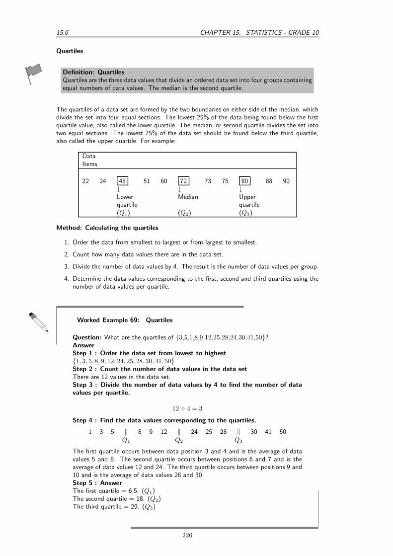
15.6 CHAPTER 15. STATISTICS - GRADE 10
Quartiles
Definition: QuartilesQuartiles are the three data values that divide an ordered data set into four groups containingequal numbers of data values. The median is the second quartile.
The quartiles of a data set are formed by the two boundaries on either side of the median, whichdivide the set into four equal sections. The lowest 25% of the data being found below the firstquartile value, also called the lower quartile. The median, or second quartile divides the set intotwo equal sections. The lowest 75% of the data set should be found below the third quartile,also called the upper quartile. For example:
DataItems
22 24 48 51 60 72 73 75 80 88 90↓ ↓ ↓Lowerquartile
Median Upperquartile
(Q1) (Q2) (Q3)
Method: Calculating the quartiles
1. Order the data from smallest to largest or from largest to smallest.
2. Count how many data values there are in the data set.
3. Divide the number of data values by 4. The result is the number of data values per group.
4. Determine the data values corresponding to the first, second and third quartiles using thenumber of data values per quartile.
Worked Example 69: Quartiles
Question: What are the quartiles of {3,5,1,8,9,12,25,28,24,30,41,50}?AnswerStep 1 : Order the data set from lowest to highest{1, 3, 5, 8, 9, 12, 24, 25, 28, 30, 41, 50}Step 2 : Count the number of data values in the data setThere are 12 values in the data set.Step 3 : Divide the number of data values by 4 to find the number of datavalues per quartile.
12 ÷ 4 = 3
Step 4 : Find the data values corresponding to the quartiles.
1 3 5 ‖ 8 9 12 ‖ 24 25 28 ‖ 30 41 50Q1 Q2 Q3
The first quartile occurs between data position 3 and 4 and is the average of datavalues 5 and 8. The second quartile occurs between positions 6 and 7 and is theaverage of data values 12 and 24. The third quartile occurs between positions 9 and10 and is the average of data values 28 and 30.Step 5 : AnswerThe first quartile = 6,5. (Q1)The second quartile = 18. (Q2)The third quartile = 29. (Q3)
226

CHAPTER 15. STATISTICS - GRADE 10 15.6
Inter-quartile Range
Definition: Inter-quartile RangeThe inter quartile range is a measure which provides information about the spread of a dataset, and is calculated by subtracting the first quartile from the third quartile, giving therange of the middle half of the data set, trimming off the lowest and highest quarters, i.e.Q3 − Q1.
The semi-interquartile range is half the interquartile range, i.e. Q3−Q1
2
Worked Example 70: Medians, Quartiles and the Interquartile Range
Question: A class of 12 students writes a test and the results are as follows: 20, 39,40, 43, 43, 46, 53, 58, 63, 70, 75, 91. Find the range, quartiles and the InterquartileRange.AnswerStep 1 :
20 39 40 ‖ 43 43 46 ‖ 53 58 63 ‖ 70 75 91Q1 M Q3
Step 2 : The RangeThe range = 91 - 20 = 71. This tells us that the marks are quite widely spread.Step 3 : The median lies between the 6th and 7th marki.e. M = 46+53
2 = 992 = 49,5
Step 4 : The lower quartile lies between the 3rd and 4th marki.e. Q1 = 40+43
2 = 832 = 41,5
Step 5 : The upper quartile lies between the 9th and 10th marki.e. Q3 = 63+70
2 = 1332 = 66,5
Step 6 : Analysing the quartilesThe quartiles are 41,5, 49,5 and 66,5. These quartiles tell us that 25% of the marksare less than 41,5; 50% of the marks are less than 49,5 and 75% of the marks areless than 66,5. They also tell us that 50% of the marks lie between 41,5 and 66,5.Step 7 : The Interquartile RangeThe Interquartile Range = 66,5 - 41,5 = 25. This tells us that the width of themiddle 50% of the data values is 25.Step 8 : The Semi-interquatile RangeThe Semi-interquartile Range = 25
2 = 12,5
Percentiles
Definition: PercentilesPercentiles are the 99 data values that divide a data set into 100 groups.
The calculation of percentiles is identical to the calculation of quartiles, except the aim is todivide the data values into 100 groups instead of the 4 groups required by quartiles.
Method: Calculating the percentiles
1. Order the data from smallest to largest or from largest to smallest.
2. Count how many data values there are in the data set.
227

15.6 CHAPTER 15. STATISTICS - GRADE 10
3. Divide the number of data values by 100. The result is the number of data values pergroup.
4. Determine the data values corresponding to the first, second and third quartiles using thenumber of data values per quartile.
15.6.3 Exercises - Summarising Data
1. Three sets of data are given:
A Data set 1: 9 12 12 14 16 22 24
B Data set 2: 7 7 8 11 13 15 16 16
C Data set 3: 11 15 16 17 19 19 22 24 27
For each one find:
i. the range
ii. the lower quartile
iii. the interquartile range
iv. the semi-interquartile range
v. the median
vi. the upper quartile
2. There is 1 sweet in one jar, and 3 in the second jar. The mean number of sweets in thefirst two jars is 2.
A If the mean number in the first three jars is 3, how many are there in the third jar?
B If the mean number in the first four jars is 4, how many are there in the fourth jar?
C If the mean number in the first n jars is n, how many are there in the n jar?
3. Find a set of five ages for which the mean age is 5, the modal age is 2 and the medianage is 3 years.
4. Four friends each have some marbles. They work out that the mean number of marblesthey have is 10. One of them leaves. She has 4 marbles. How many marbles do theremaining friends have together?
Worked Example 71: Mean, Median and Mode for Grouped Data
Question:Consider the following grouped data and calculate the mean, the modal group andthe median group.
Mass (kg) Frequency41 - 45 746 - 50 1051 - 55 1556 - 60 1261 - 65 6
Total = 50
AnswerStep 1 : Calculating the meanTo calculate the mean we need to add up all the masses and divide by 50. We do notknow actual masses, so we approximate by choosing the midpoint of each group.We then multiply those midpoint numbers by the frequency. Then we add thesenumbers together to find the approximate total of the masses. This is show in thetable below.
228

CHAPTER 15. STATISTICS - GRADE 10 15.7
Mass (kg) Midpoint Frequency Midpt × Freq41 - 45 (41+45)/2 = 43 7 43 × 7 = 30146 - 50 48 10 48051 - 55 53 15 79556 - 60 58 12 69661 - 65 63 6 378
Total = 50 Total = 2650
Step 2 : AnswerThe mean = 2650
50 = 53.The modal group is the group 51 - 53 because it has the highest frequency.The median group is the group 51 - 53, since the 25th and 26th terms are containedwithin this group.
Exercise: More mean, modal and median group exercises.In each data set given, find the mean, the modal group and the median group.
1. Times recorded when learners played a game.
Time in seconds Frequency
36 - 45 546 - 55 1156 - 65 1566 - 75 2676 - 85 1986 - 95 1396 - 105 6
2. The following data were collected from a group of learners.
Mass in kilograms Frequency
41 - 45 346 - 50 551 - 55 856 - 60 1261 - 65 1466 - 70 971 - 75 776 - 80 2
15.7 Misuse of Statistics
In many cases groups can gain an advantage by misleading people with the misuse of statistics.
Common techniques used include:
• Three dimensional graphs.
• Axes that do not start at zero.
229

15.7 CHAPTER 15. STATISTICS - GRADE 10
• Axes without scales.
• Graphic images that convey a negative or positive mood.
• Assumption that a correlation shows a necessary causality.
• Using statistics that are not truly representative of the entire population.
• Using misconceptions of mathematical concepts
For example, the following pairs of graphs show identical information but look very different.Explain why.
0
5
10
15
20
JFMAMJJ
0
5
10
15
20
J F M A M J J
0
2
4
6
8
10
Option 1 Option 27
8
9
10
Option 1 Option 2
MonthsMonths
15.7.1 Exercises - Misuse of Statistics
1. A company has tried to give a visual representation of the increase in their earnings fromone year to the next. Does the graph below convince you? Critically analyse the graph.
2006 2007
2. In a study conducted on a busy highway, data was collected about drivers breaking thespeed limit and the colour of the car they were driving. The data were collected during a20 minute time interval during the middle of the day, and are presented in a table and piechart below.
Colour of carFrequency ofdrivers speeding
White 22
Blue 10
Red 8
Blue
Red
White
230

CHAPTER 15. STATISTICS - GRADE 10 15.7
Conclusions made by a novice based on the data are summarised as follows:
“People driving white cars are more likely to break the speed limit.”
“Drivers in blue and red cars are more likely to stick to the speed limit.”
Do you agree with these conclusions? Explain.
3. A record label produces a graphic, showing their advantage in sales over their competi-tors. Identify at least three devices they have used to influence and mislead the readersimpression.
50 million copies
40 million copies
Our sales Competitor’s sales
4. In an effort to discredit their competition, a tour bus company prints the graph shownbelow. Their claim is that the competitor is losing business. Can you think of a betterexplanation?
0
400
800
1200
1600
2000
2400
O N D J F M A M J
Months of 2006/2007
Nu
mb
ero
fto
uri
stp
asse
ng
ers
5. The caption from a newspaper article quoted below, demonstrates a misuse of statisticalconcepts. Explain.
“More than 40% of learners in South Africa are below average in mathematics.”
6. To test a theory, 8 different offices were monitored for noise levels and productivity of theemployees in the office. The results are graphed below.
Pro
duct
ivity
Noise Level
×
×
××
×
××
Noise Level vs Productivity
231

15.8 CHAPTER 15. STATISTICS - GRADE 10
The following statement was then made:“If an office environment is noisy, this leads to poor productivity.”
Explain the flaws in this thinking.
15.8 Summary of Definitions
mean The mean of a data set, x, denoted by x, is the average of the data values, and iscalculated as:
x =sum of values
number of values(15.2)
median The median is the centre data value in a data set that has been ordered from lowest tohighest
mode The mode is the data value that occurs most often in a data set.
15.9 Exercises
1. “Using the median size as a reference, you would be able to fit four 1 cent coins and a carinto a match box.” Explain why this statement is true.
2. Calculate the mean, median, and mode of Data Set 3.
3. The tallest 7 trees in a park have heights in metres of 41, 60, 47, 42, 44, 42, and 47. Findthe median of their heights.
4. The students in Bjorn’s class have the following ages: 5, 9, 1, 3, 4, 6, 6, 6, 7, 3. Find themode of their ages.
5. The masses (in kg, correct to the nearest 0,1 kg) of thirty people were measured as follows:
45,1 57,9 67,9 57,4 50,7 61,1 63,9 67,5 69,7 71,768,0 63,2 58,7 56,9 78,5 59,7 54,4 66,4 51,6 47,770,9 54,8 59,1 60,3 60,1 52,6 74,9 72,1 49,5 49,8
A Copy the frequency table below, and complete it.
Mass (in kg) Tally Number of people45,0 ≤ m < 50,050,0 ≤ m < 55,055,0 ≤ m < 60,060,0 ≤ m < 65,065,0 ≤ m < 70,070,0 ≤ m < 75,075,0 ≤ m < 80,0
B Draw a frequency polygon for this information.
C What can you conclude from looking at the graph?
6. An engineering company has designed two different types of engines for motorbikes. Thetwo different motorbikes are tested for the time it takes (in seconds) for them to acceleratefrom 0 km/h to 60 km/h.
Test1
Test2
Test3
Test4
Test5
Test6
Test7
Test8
Test9
Test10
Average
Bike1
1.55 1.00 0.92 0.80 1.49 0.71 1.06 0.68 0.87 1.09
Bike2
0.9 1.0 1.1 1.0 1.0 0.9 0.9 1.0 0.9 1.1
A What kind of average should be used for this information?
B Calculate the average you chose in the previous question for each motorbike.
232

CHAPTER 15. STATISTICS - GRADE 10 15.9
C Which motorbike would you choose based on this information? Take note of accuracyof the numbers from each set of tests.
D How far will a motorbike travelling at 60 km/h travel in 1 second?
7. The heights of 40 learners are given below.
154 140 145 159 150 132 149 150 138 152141 132 169 173 139 161 163 156 157 171168 166 151 152 132 142 170 162 146 152142 150 161 138 170 131 145 146 147 160
A Set up a frequency table using 6 intervals.
B Calculate the approximate mean.
C Determine the mode.
D Determin the modal class.
E How many learners are taller than your approximate average in (b)?
8. In a traffic survey, a random sample of 50 motorists were asked the distance they drove towork daily. This information is shown in the table below.
Distance in km 1-5 6-10 11-15 16-20 21-25 26-30 31-35 36-40 41-45Frequency 4 5 9 10 7 8 3 2 2
A Find the approximate mean.
B Find the modal class.
C What percentage of samples drove
i. less than 16 km?
ii. more than 30 km?
iii. between 16 km and 30 km daily?
9. A company wanted to evaluate the training programme in its factory. They gave the sametask to trained and untrained employees and timed each one in seconds.
Trained 121 137 131 135 130128 130 126 132 127129 120 118 125 134
Untrained 135 142 126 148 145156 152 153 149 145144 134 139 140 142
A Draw a back-to-back stem and leaf diagram to show the two sets of data.
B Find the medians and quartiles for both sets of data.
C Find the Interquartile Range for both sets of data.
D Comment on the results.
10. A small firm employs nine people. The annual salaries of the employers are:
R600 000 R250 000 R200 000R120 000 R100 000 R100 000R100 000 R90 000 R80 000
A Find the mean of these salaries.
B Find the mode.
C Find the median.
D Of these three figures, which would you use for negotiating salary increases if youwere a trade union official? Why?
233

15.9 CHAPTER 15. STATISTICS - GRADE 10
11. The marks for a particular class test are listed here:
67 58 91 67 58 82 71 51 60 8431 67 96 64 78 71 87 78 89 3869 62 60 73 60 87 71 49
A Complete the frequency table using the given class intervals.
Class Tally Frequency Mid-point Freq × Midpt30-39 34,540-49 44,550-5960-6970-7980-8990-99
Sum = Sum =
234

Chapter 16
Probability - Grade 10
16.1 Introduction
Very little in mathematics is truly self-contained. Many branches of mathematics touch andinteract with one another, and the fields of probability and statistics are no different. A basicunderstanding of probability is vital in grasping basic statistics, and probability is largely abstractwithout statistics to determine the ”real world” probabilities.
Probability theory is concerned with predicting statistical outcomes. A simple example of astatistical outcome is observing a head or tail when tossing a coin. Another simple example of astatistical outcome is obtaining the numbers 1, 2, 3, 4, 5, or 6 when rolling a die. (We say onedie, many dice.)
For a fair coin, heads should occur for 12 of the number of tosses and for a fair die, each number
should occur for 16 of the number of rolls. Therefore, the probability of observing a head on one
toss of a fair coin is 12 and that for obtaining a four on one roll of a fair die is 1
6 .
In earlier grades, the idea has been introduced that different situations have different probabilitiesof occurring and that for many situations there are a finite number of different possible outcomes.In general, events from daily life can be classified as either:
• certain that they will happen; or
• certain that they will not happen; or
• uncertain.
This chapter builds on earlier work and describes how to calculate the probability associated withdifferent situations, and describes how probability is used to assign a number describing the levelof chance or the odds associated with aspects of life. The meanings of statements like: ‘TheHIV test is 85% reliable.’ will also be explained.
16.2 Random Experiments
The term random experiment or statistical experiment is used to describe any repeatable exper-iment or situation, with individual experiments having one of a set of outcomes or results. A setof outcomes is known as an event. For example, the act of tossing a coin or rolling a die canbe considered to be simple random experiments. With the results of either a heads or tails orone of {1,2,3,4,5,6} being the outcomes. These experiments are repeatable and yield differentoutcomes each time.
16.2.1 Sample Space of a Random Experiment
The set of all possible outcomes in a random experiment plays an important role in probabilitytheory and is known as the sample space. The letter S is used to indicate the sample space.
235

16.2 CHAPTER 16. PROBABILITY - GRADE 10
Using the terminology of set theory, the elements of S are then the outcomes of the randomexperiment. For example, when tossing a coin the sample space S is made up of {heads,tails}.
Worked Example 72: Sample Space
Question: What outcomes make up the sample space S when rolling a die.AnswerStep 3 : Determine all the possible outcomesThe possible outcomes when rolling a die are: 1, 2, 3, 4, 5 and 6.Step 4 : Define the sample space, SFor rolling a die, the sample space is S = {1,2,3,4,5,6}.
A set of outcomes is referred to as an event. For example, when rolling a die the outcomes thatare an even number (i.e. {2,4,6}) would be referred to as an event. It is clear that outcomesand events are subsets of the sample space, S.
A Venn diagram can be used to show the relationship between the outcomes of a randomexperiment, the sample space and events associated with the outcomes. The Venn diagramin Figure 16.1 shows the difference between the universal set, a sample space and events andoutcomes as subsets of the sample space.
Universal set
Sample space, S
Event A
Event B
Figure 16.1: Diagram to show difference between the universal set and the sample space. Thesample space is made up of all possible outcomes of a statistical experiment and an event is asubset of the sample space.
Venn diagrams can also be used to indicate the union and intersection between events in asample space (Figure 16.2).
Worked Example 73: Random Experiments
Question: In a box there are pieces of paper with the numbers from 1 to 9 writtenon them.S = {1; 2; 3; 4; 5; 6; 7; 8; 9}AnswerStep 1 : Consider the events:
• Drawing a prime number; P = {2, 3, 5, 7}236

CHAPTER 16. PROBABILITY - GRADE 10 16.2
Event, A Event, B
Sample space, S
Event A Event B
Sample Space S
Figure 16.2: Venn diagram to show (left) union of two events, A and B, in the sample space Sand (right) intersection of two events A and B, in the sample space S. The crosshatched regionindicates the intersection.
• Drawing an even number; E = {2, 4, 6, 8}Step 2 : Draw a diagram
S
EP
12
3
45
67
8
9
Step 3 : Find the unionThe union of P and E is the set of all elements in P or in E (or in both). P or E =2, 3, 4, 5, 6, 7, 8. P or E is also written P ∪ E.Step 4 : Find the intersectionThe intersection of P and E is the set of all elements in both P and E. P and E =2. P and E is also written as P ∩ E.Step 5 : Find the number in each setWe use n(S) to refer to the number of elements in a set S, n(X) for the numberof elements in X , etc.
∴ n(S) = 9
n(P ) = 4
n(E) = 4
n(P ∪ E) = 7
n(P ∩ E) = 2
237

16.3 CHAPTER 16. PROBABILITY - GRADE 10
Exercise: Random Experiments
1. S = {whole numbers from 1 to 16}, X = {even numbers from 1 to 16} andY = {prime numbers from 1 to 16}
A Draw a Venn diagram S, X and Y .
B Write down n(S), n(X), n(Y ), n(X ∪ Y ), n(X ∩ Y ).
2. There are 79 Grade 10 learners at school. All of these take either Maths,Geography or History. The number who take Geography is 41, those who takeHistory is 36, and 30 take Maths. The number who take Maths and Historyis 16; the number who take Geography and History is 6, and there are 8 whotake Maths only and 16 who take only History.
A Draw a Venn diagram to illustrate all this information.
B How many learners take Maths and Geography but not History?
C How many learners take Geography only?
D How many learners take all three subjects?
3. Pieces of paper labelled with the numbers 1 to 12 are placed in a box and thebox is shaken. One piece of paper is taken out and then replaced.
A What is the sample space, S?
B Write down the set A, representing the event of taking a piece of paperlabelled with a factor 12.
C Write down the set B, representing the event of taking a piece of paperlabelled with a prime number.
D Represent A, B and S by means of a Venn diagram.
E Write down
i. n(S)
ii. n(A)
iii. n(B)
iv. n(A ∩ B)
v. n(A ∪ B)
F Is n(A ∪ B) = n(A) + n(B) − n(A ∩ B)?
16.3 Probability Models
The word probability relates to uncertain events or knowledge, being closely related in meaningto likely, risky, hazardous, and doubtful. Chance, odds, and bet are other words expressing similarideas.
Probability is connected with uncertainty. In any statistical experiment, the outcomes that occurmay be known, but exactly which one might not be known. Mathematically, probability theoryformulates incomplete knowledge pertaining to the likelihood of an occurrence. For example, ameteorologist might say there is a 60% chance that it will rain tomorrow. This means that in 6of every 10 times when the world is in the current state, it will rain.
A probability is a real number between 0 and 1. In everyday speech, probabilities are usually givenas a percentage between 0% and 100%. A probability of 100% means that an event is certain,whereas a probability of 0% is often taken to mean the event is impossible. However, there isa distinction between logically impossible and occurring with zero probability; for example, inselecting a number uniformly between 0 and 1, the probability of selecting 1/2 is 0, but it isnot logically impossible. Further, it is certain that whichever number is selected will have had aprobability of 0 of being selected.
Another way of referring to probabilities is odds. The odds of an event is defined as the ratioof the probability that the event occurs to the probability that it does not occur. For example,the odds of a coin landing on a given side are 0.5
0.5 = 1, usually written ”1 to 1” or ”1:1”. Thismeans that on average, the coin will land on that side as many times as it will land on the otherside.
238

CHAPTER 16. PROBABILITY - GRADE 10 16.3
16.3.1 Classical Theory of Probability
1. Equally likely outcomes are outcomes which have an equal chance of happening. Forexample when a fair coin is tossed, each outcome in the sample space S = heads, tails isequally likely to occur.
2. When all the outcomes are equally likely (in any activity), you can calculate the probabilityof an event happening by using the following definition:P(E)=number of favourable outcomes/total number of possible outcomesP(E)=n(E)/n(S)For example, when you throw a fair dice the possible outcomes are S = {1,2,3,4,5,6} i.ethe total number of possible outcomes n(S)=6.
Event 1: get a 4The only possible outcome is a 4, i.e E=4 i.e number of favourable outcomes: n(E)=1.Probability of getting a 4 = P(4)=n(E)/n(S)=1/6.Event 2: get a number greater than 3Favourable outcomes: E = {4,5,6}Number of favourable outcomes: n(E)=3Probability of getting a number more than 3 = P(more than 3) = n(E)/n(S)=3/6=1/2
Worked Example 74: Classical Probability
Question: Various probabilities relating to a deck of cardsAnswerA standard deck of cards (without jokers) has 52 cards. If we randomly draw acard from the deck, we can think of each card as a possible outcome. Therefore,there are 52 total outcomes. We can now look at various events and calculate theirprobabilities:
1. Out of the 52 cards, there are 13 clubs. Therefore, if the event of interest isdrawing a club, there are 13 favourable outcomes, and the probability of thisevent is 13
52 = 14 .
2. There are 4 kings (one of each suit). The probability of drawing a king is452 = 1
13 .
3. What is the probability of drawing a king OR a club? This example is slightlymore complicated. We cannot simply add together the number of number ofoutcomes for each event separately (4 + 13 = 17) as this inadvertently countsone of the outcomes twice (the king of clubs). The correct answer is 16
52 .
Exercise: Probability Models
1. A bag contains 6 red, 3 blue, 2 green and 1 white balls. A ball is picked atrandom. What is the probablity that it is:
A red
B blue or white
C not green
D not green or red?
2. A card is selected randomly from a pack of 52. What is the probability that itis:
239

16.4 CHAPTER 16. PROBABILITY - GRADE 10
A the 2 of hearts
B a red card
C a picture card
D an ace
E a number less than 4?
3. Even numbers from 2 -100 are written on cards. What is the probability ofselecting a multiple of 5, if a card is drawn at random?
16.4 Relative Frequency vs. Probability
There are two approaches to determining the probability associated with any particular event ofa random experiment:
1. determining the total number of possible outcomes and calculating the probability of eachoutcome using the definition of probability
2. performing the experiment and calculating the relative frequency of each outcome
Relative frequency is defined as the number of times an event happens in a statistical experimentdivided by the number of trials conducted.
It takes a very large number of trials before the relative frequency of obtaining a head on a tossof a coin approaches the probability of obtaining a head on a toss of a coin. For example, thedata in Table 16.1 represent the outcomes of repeating 100 trials of a statistical experiment 100times, i.e. tossing a coin 100 times.
H T T H H T H H H HH H H H T H H T T TT T H T T H T H T HH H T T H T T H T TT H H H T T H T T HH T T T T H T T H HT T H T T H T T H TH T T H T T T T H TT H T T H H H T H TT T T H H T T T H T
Table 16.1: Results of 100 tosses of a fair coin. H means that the coin landed heads-up and Tmeans that the coin landed tails-up.
The following two worked examples show that the relative frequency of an event is not necessarilyequal to the probability of the same event. Relative frequency should therefore be seen as anapproximation to probability.
Worked Example 75: Relative Frequency and Probability
Question: Determine the relative frequencies associated with each outcome of thestatistical experiment detailed in Table 16.1.AnswerStep 1 : Identify the different outcomesThere are two unique outcomes: H and T.Step 2 : Count how many times each outcome occurs.
240

CHAPTER 16. PROBABILITY - GRADE 10 16.4
Outcome Frequency
H 44T 56
Step 3 : Determine the total number of trials.The statistical experiment of tossing the coin was performed 100 times. Therefore,there were 100 trials, in total.Step 4 : Calculate the relative frequency of each outcome
Probability of H =frequency of outcome
number of trials
=44
100= 0.44
Relative Frequency of T =frequency of outcome
number of trials
=56
100= 0.56
The relative frequency of the coin landing heads-up is 0.44 and the relative frequencyof the coin landing tails-up is 0.56.
Worked Example 76: Probability
Question: Determine the probability associated with an evenly weighted coin landingon either of its faces.AnswerStep 1 : Identify the different outcomesThere are two unique outcomes: H and T.Step 2 : Determine the total number of outcomes.There are two possible outcomes.Step 3 : Calculate the probability of each outcome
Relative Frequency of H =number of favourable outcomes
total number of outcomes
=1
2= 0.5
Relative Frequency of T =number of favourable outcomes
total number of outcomes
=1
2= 0.5
The probability of an evenly weighted coin landing on either face is 0.5.
241

16.5 CHAPTER 16. PROBABILITY - GRADE 10
16.5 Project Idea
Perform an experiment to show that as the number of trials increases, the relative frequencyapproaches the probability of a coin toss. Perform 10, 20, 50, 100, 200 trials of tossing a coin.
16.6 Probability Identities
The following results apply to probabilities, for the sample space S and two events A and B,within S.
P (S) = 1 (16.1)
P (A ∩ B) = P (A) × P (B) (16.2)
P (A ∪ B) = P (A) + P (B) − P (A ∩ B) (16.3)
Worked Example 77: Probabilty identitys
Question: What is the probability of selecting a black or red card from a pack of52 cardsAnswerP(S)=n(E)/n(S)=52/52=1. because all cards are black or red!
Worked Example 78: Probabilty identitys
Question: What is the probability of drawing a club or an ace with one single pickfrom a pack of 52 cardsAnswerStep 1 : Identify the identity which describes the situation
P (club ∪ ace) = P (club) + P (ace) − P (club ∩ ace)
Step 2 : Calculate the answer
=1
4+
1
13−
(
1
4× 1
13
)
=1
4+
1
13− 1
52
=16
52
=4
13
Notice how we have used P (C ∪ A) = P (C) + P (A) − P (C ∩ A).
242

CHAPTER 16. PROBABILITY - GRADE 10 16.7
Exercise: Probability IdentitiesAnswer the following questions
1. Rory is target shooting. His probability of hitting the target is 0.7. He fires five shots.What is the probability that:
A All five shots miss the center?
B At least 3 shots hit the center?
2. An archer is shooting arrows at a bullseye. The probability that an arrow hits the bullseyeis 0.4. If she fires three arrows, what is the probability that:
A All the arrows hit the bullseye,
B only one of the arrows hit the bullseye?
3. A dice with the numbers 1,3,5,7,9,11 on it is rolled. Also a fair coin is tossed.
A Draw a sample space diagram to show all outcomes.
B What is the probability that:
i. A tail is tossed and a 9 rolled?
ii. A head is tossed and a 3 rolled?
4. Four children take a test. The probability of each one passing is as follows. Sarah: 0.8,Kosma: 0.5, Heather: 0.6, Wendy: 0.9. What is the probability that:
A all four pass?
B all four fail?
C at least one passes?
5. With a single pick from a pack of 52 cards what is the probability that the card will be anace or a black card?
16.7 Mutually Exclusive Events
Mutually exclusive events are events, which cannot be true at the same time.
Examples of mutually exclusive events are:
1. A die landing on an even number or landing on an odd number.
2. A student passing or failing an exam
3. A tossed coin landing on heads or landing on tails
This means that if we examine the elements of the sets that make up A and B there will beno elements in common. Therefore, A ∩ B = ∅ (where ∅ refers to the empty set). Since,P (A ∩ B) = 0, equation 16.3 becomes:
P (A ∪ B) = P (A) + P (B)
for mutually exclusive events.
243

16.8 CHAPTER 16. PROBABILITY - GRADE 10
Exercise: Mutually Exclusive EventsAnswer the following questions
1. A box contains coloured blocks. The number of each colour is given in the following table.
Colour Purple Orange White PinkNumber of blocks 24 32 41 19
A block is selected randomly. What is the probability that the block will be:
A purple
B purple or white
C pink and orange
D not orange?
2. A small private school has a class with children of various ages. The table gies the numberof pupils of each age in the class.
3 years female 3 years male 4 years female 4 years male 5 years female 5 years male6 2 5 7 4 6
If a pupil is selceted at random what is the probability that the pupil will be:
A a female
B a 4 year old male
C aged 3 or 4
D aged 3 and 4
E not 5
F either 3 or female?
3. Fiona has 85 labeled discs, which are numbered from 1 to 85. If a disc is selected atrandom what is the probability that the disc number:
A ends with 5
B can be multiplied by 3
C can be multiplied by 6
D is number 65
E is not a multiple of 5
F is a multiple of 4 or 3
G is a multiple of 2 and 6
H is number 1?
16.8 Complementary Events
The probability of complementary events refers to the probability associated with events notoccurring. For example, if P (A) = 0.25, then the probability of A not occurring is the probabilityassociated with all other events in S occurring less the probability of A occurring. This meansthat
P (A′) = 1 − P (A)
where A’ refers to ‘not A’ In other words, the probability of ‘not A’ is equal to one minus theprobability of A.
244

CHAPTER 16. PROBABILITY - GRADE 10 16.8
Worked Example 79: Probability
Question: If you throw two dice, one red and one blue, what is the probability thatat least one of them will be a six?AnswerStep 1 : Work out probability of event 1To solve that kind of question, work out the probability that there will be no six.Step 2 : Work out probability of event 2The probability that the red dice will not be a six is 5/6, and that the blue one willnot be a six is also 5/6.Step 3 : Probability of neitherSo the probability that neither will be a six is 5/6 × 5/6 = 25/36.Step 4 : Probability of oneSo the probability that at least one will be a six is 1 − 25/36 = 11/36.
Worked Example 80: Probability
Question: A bag contains three red balls, five white balls, two green balls and fourblue balls:1. Calculate the probability that a red ball will be drawn from the bag.2. Calculate the probability that a ball which is not red will be drawnAnswerStep 1 : Find event 1Let R be the event that a red ball is drawn:
• P(R)-n(R)/n(S)=3/14
• R and R’ are complementary events
Step 2 : Find the probabilitys∴ P(R’) = 1 - P(R) = 1 -3/14 = 11/14Step 3 : Alternate way to solve it
• Alternately P(R’) = P(B) + P(W) + P(G)
• P(R’) = 4/14 + 5/14 + 2/14 = 11/14
Extension: Interpretation of Probability ValuesThe probability of an event is generally represented as a real number between 0 and1, inclusive. An impossible event has a probability of exactly 0, and a certain eventhas a probability of 1, but the converses are not always true: probability 0 events arenot always impossible, nor probability 1 events certain. The rather subtle distinctionbetween ”certain” and ”probability 1” is treated at greater length in the article on”almost surely”.
Most probabilities that occur in practice are numbers between 0 and 1, indicatingthe event’s position on the continuum between impossibility and certainty. The closeran event’s probability is to 1, the more likely it is to occur.
For example, if two mutually exclusive events are assumed equally probable, suchas a flipped or spun coin landing heads-up or tails-up, we can express the probabilityof each event as ”1 in 2”, or, equivalently, ”50%” or ”1/2”.
245

16.9 CHAPTER 16. PROBABILITY - GRADE 10
Probabilities are equivalently expressed as odds, which is the ratio of the proba-bility of one event to the probability of all other events. The odds of heads-up, forthe tossed/spun coin, are (1/2)/(1 - 1/2), which is equal to 1/1. This is expressedas ”1 to 1 odds” and often written ”1:1”.
Odds a:b for some event are equivalent to probability a/(a+b). For example, 1:1odds are equivalent to probability 1/2, and 3:2 odds are equivalent to probability3/5.
16.9 End of Chapter Exercises
1. A group of 45 children were asked if they eat Frosties and/or Strawberry Pops. 31 eatboth and 6 eat only Frosties. What is the probability that a child chosen at random willeat only Strawberry Pops?
2. In a group of 42 pupils, all but 3 had a packet of chips or a Fanta or both. If 23 hada packet of chips and 7 of these also had a Fanta, what is the probability that one pupilchosen at random has:
A Both chips and Fanta
B has only Fanta?
3. Use a Venn diagram to work out the following probabilities from a die being rolled:
A A multiple of 5 and an odd number
B a number that is neither a multiple of 5 nor an odd number
C a number which is not a multiple of 5, but is odd.
4. A packet has yellow and pink sweets. The probability of taking out a pink sweet is 7/12.
A What is the probability of taking out a yellow sweet
B If 44 if the sweets are yellow, how many sweets are pink?
5. In a car park with 300 cars, there are 190 Opals. What is the probability that the first carto leave the car park is:
A an Opal
B not an Opal
6. Tamara has 18 loose socks in a drawer. Eight of these are orange and two are pink.Calculate the probability that the first sock taken out at random is:
A Orange
B not orange
C pink
D not pink
E orange or pink
F not orange or pink
7. A plate contains 9 shortbread cookies, 4 ginger biscuits, 11 chocolate chip cookies and 18Jambos. If a biscuit is selected at random, what is the probability that:
A it is either a ginger biscuit of a Jambo?
B it is NOT a shortbread cookie.
8. 280 tickets were sold at a raffle. Ingrid bought 15 tickets. What is the probability thatIngrid:
A Wins the prize
B Does not win the prize?
246

CHAPTER 16. PROBABILITY - GRADE 10 16.9
9. The children in a nursery school were classified by hair and eye colour. 44 had red hairand not brown eyes, 14 had brown eyes and red hair, 5 had brown eyes but not red hairand 40 did not have brown eyes or red hair.
A How many children were in the school
B What is the probility that a child chosen at random has:
i. Brown eyes
ii. Red hair
C A child with brown eyes is chosen randomly. What is the probability that this childwill have red hair
10. A jar has purple, blue and black sweets in it. The probability that a sweet, chosen atrandom, will be purple is 1/7 and the probability that it will be black is 3/5.
A If I choose a sweet at random what is the probability that it will be:
i. purple or blue
ii. Black
iii. purple
B If there are 70 sweets in the jar how many purple ones are there?
C 1/4 if the purple sweets in b) have streaks on them and rest do not. How manypurple sweets have streaks?
11. For each of the following, draw a Venn diagram to represent the situation and find anexample to illustrate the situation.
A A sample space in which there are two events that are not mutually exclusive
B A sample space in which there are two events that are complementary.
12. Use a Venn diagram to prove that the probability of either event A or B occuring is givenby: (A and B are not exclusive)P(A or B) = P(A) + P(B) - P(A and B)
13. All the clubs are taken out of a pack of cards. The remaining cards are then shuffled andone card chosen. After being chosen, the card is replaced before the next card is chosen.
A What is the sample space?
B Find a set to represent the event, P, of drawing a picture card.
C Find a set for the event, N, of drawing a numbered card.
D Represent the above events in a Venn diagram
E What description of the sets P and N is suitable? (Hint: Find any elements of P inN and N in P.)
14. Thuli has a bag containing five orange, three purple and seven pink blocks. The bagis shaken and a block is withdrawn. The colour of the block is noted and the block isreplaced.
A What is the sample space for this experiment?
B What is the set describing the event of drawing a pink block, P?
C Write down a set, O or B, to represent the event of drawing either a orange or apurple block.
D Draw a Venn diagram to show the above information.
247

16.9 CHAPTER 16. PROBABILITY - GRADE 10
248

Appendix A
GNU Free Documentation License
Version 1.2, November 2002Copyright c© 2000,2001,2002 Free Software Foundation, Inc.59 Temple Place, Suite 330, Boston, MA 02111-1307 USAEveryone is permitted to copy and distribute verbatim copies of this license document, butchanging it is not allowed.
PREAMBLE
The purpose of this License is to make a manual, textbook, or other functional and useful doc-ument “free” in the sense of freedom: to assure everyone the effective freedom to copy andredistribute it, with or without modifying it, either commercially or non-commercially. Secondar-ily, this License preserves for the author and publisher a way to get credit for their work, whilenot being considered responsible for modifications made by others.
This License is a kind of “copyleft”, which means that derivative works of the document mustthemselves be free in the same sense. It complements the GNU General Public License, whichis a copyleft license designed for free software.
We have designed this License in order to use it for manuals for free software, because freesoftware needs free documentation: a free program should come with manuals providing thesame freedoms that the software does. But this License is not limited to software manuals; itcan be used for any textual work, regardless of subject matter or whether it is published as aprinted book. We recommend this License principally for works whose purpose is instruction orreference.
APPLICABILITY AND DEFINITIONS
This License applies to any manual or other work, in any medium, that contains a notice placedby the copyright holder saying it can be distributed under the terms of this License. Such anotice grants a world-wide, royalty-free license, unlimited in duration, to use that work underthe conditions stated herein. The “Document”, below, refers to any such manual or work. Anymember of the public is a licensee, and is addressed as “you”. You accept the license if youcopy, modify or distribute the work in a way requiring permission under copyright law.
A “Modified Version” of the Document means any work containing the Document or a portionof it, either copied verbatim, or with modifications and/or translated into another language.
A “Secondary Section” is a named appendix or a front-matter section of the Document that dealsexclusively with the relationship of the publishers or authors of the Document to the Document’soverall subject (or to related matters) and contains nothing that could fall directly within thatoverall subject. (Thus, if the Document is in part a textbook of mathematics, a SecondarySection may not explain any mathematics.) The relationship could be a matter of historicalconnection with the subject or with related matters, or of legal, commercial, philosophical,ethical or political position regarding them.
619

APPENDIX A. GNU FREE DOCUMENTATION LICENSE
The “Invariant Sections” are certain Secondary Sections whose titles are designated, as beingthose of Invariant Sections, in the notice that says that the Document is released under thisLicense. If a section does not fit the above definition of Secondary then it is not allowed to bedesignated as Invariant. The Document may contain zero Invariant Sections. If the Documentdoes not identify any Invariant Sections then there are none.
The “Cover Texts” are certain short passages of text that are listed, as Front-Cover Texts orBack-Cover Texts, in the notice that says that the Document is released under this License. AFront-Cover Text may be at most 5 words, and a Back-Cover Text may be at most 25 words.
A “Transparent” copy of the Document means a machine-readable copy, represented in a formatwhose specification is available to the general public, that is suitable for revising the documentstraightforwardly with generic text editors or (for images composed of pixels) generic paintprograms or (for drawings) some widely available drawing editor, and that is suitable for inputto text formatters or for automatic translation to a variety of formats suitable for input to textformatters. A copy made in an otherwise Transparent file format whose markup, or absence ofmarkup, has been arranged to thwart or discourage subsequent modification by readers is notTransparent. An image format is not Transparent if used for any substantial amount of text. Acopy that is not “Transparent” is called “Opaque”.
Examples of suitable formats for Transparent copies include plain ASCII without markup, Texinfoinput format, LATEX input format, SGML or XML using a publicly available DTD and standard-conforming simple HTML, PostScript or PDF designed for human modification. Examples oftransparent image formats include PNG, XCF and JPG. Opaque formats include proprietaryformats that can be read and edited only by proprietary word processors, SGML or XML forwhich the DTD and/or processing tools are not generally available, and the machine-generatedHTML, PostScript or PDF produced by some word processors for output purposes only.
The “Title Page” means, for a printed book, the title page itself, plus such following pages asare needed to hold, legibly, the material this License requires to appear in the title page. Forworks in formats which do not have any title page as such, “Title Page” means the text near themost prominent appearance of the work’s title, preceding the beginning of the body of the text.
A section “Entitled XYZ” means a named subunit of the Document whose title either is preciselyXYZ or contains XYZ in parentheses following text that translates XYZ in another language.(Here XYZ stands for a specific section name mentioned below, such as “Acknowledgements”,“Dedications”, “Endorsements”, or “History”.) To “Preserve the Title” of such a section whenyou modify the Document means that it remains a section “Entitled XYZ” according to thisdefinition.
The Document may include Warranty Disclaimers next to the notice which states that thisLicense applies to the Document. These Warranty Disclaimers are considered to be included byreference in this License, but only as regards disclaiming warranties: any other implication thatthese Warranty Disclaimers may have is void and has no effect on the meaning of this License.
VERBATIM COPYING
You may copy and distribute the Document in any medium, either commercially or non-commercially,provided that this License, the copyright notices, and the license notice saying this License appliesto the Document are reproduced in all copies, and that you add no other conditions whatsoeverto those of this License. You may not use technical measures to obstruct or control the readingor further copying of the copies you make or distribute. However, you may accept compensationin exchange for copies. If you distribute a large enough number of copies you must also followthe conditions in section A.
You may also lend copies, under the same conditions stated above, and you may publicly displaycopies.
COPYING IN QUANTITY
If you publish printed copies (or copies in media that commonly have printed covers) of theDocument, numbering more than 100, and the Document’s license notice requires Cover Texts,
620

APPENDIX A. GNU FREE DOCUMENTATION LICENSE
you must enclose the copies in covers that carry, clearly and legibly, all these Cover Texts: Front-Cover Texts on the front cover, and Back-Cover Texts on the back cover. Both covers must alsoclearly and legibly identify you as the publisher of these copies. The front cover must present thefull title with all words of the title equally prominent and visible. You may add other material onthe covers in addition. Copying with changes limited to the covers, as long as they preserve thetitle of the Document and satisfy these conditions, can be treated as verbatim copying in otherrespects.
If the required texts for either cover are too voluminous to fit legibly, you should put the firstones listed (as many as fit reasonably) on the actual cover, and continue the rest onto adjacentpages.
If you publish or distribute Opaque copies of the Document numbering more than 100, you musteither include a machine-readable Transparent copy along with each Opaque copy, or state in orwith each Opaque copy a computer-network location from which the general network-using publichas access to download using public-standard network protocols a complete Transparent copy ofthe Document, free of added material. If you use the latter option, you must take reasonablyprudent steps, when you begin distribution of Opaque copies in quantity, to ensure that thisTransparent copy will remain thus accessible at the stated location until at least one year afterthe last time you distribute an Opaque copy (directly or through your agents or retailers) of thatedition to the public.
It is requested, but not required, that you contact the authors of the Document well beforeredistributing any large number of copies, to give them a chance to provide you with an updatedversion of the Document.
MODIFICATIONS
You may copy and distribute a Modified Version of the Document under the conditions ofsections A and A above, provided that you release the Modified Version under precisely thisLicense, with the Modified Version filling the role of the Document, thus licensing distributionand modification of the Modified Version to whoever possesses a copy of it. In addition, youmust do these things in the Modified Version:
1. Use in the Title Page (and on the covers, if any) a title distinct from that of the Document,and from those of previous versions (which should, if there were any, be listed in the Historysection of the Document). You may use the same title as a previous version if the originalpublisher of that version gives permission.
2. List on the Title Page, as authors, one or more persons or entities responsible for authorshipof the modifications in the Modified Version, together with at least five of the principalauthors of the Document (all of its principal authors, if it has fewer than five), unless theyrelease you from this requirement.
3. State on the Title page the name of the publisher of the Modified Version, as the publisher.
4. Preserve all the copyright notices of the Document.
5. Add an appropriate copyright notice for your modifications adjacent to the other copyrightnotices.
6. Include, immediately after the copyright notices, a license notice giving the public permis-sion to use the Modified Version under the terms of this License, in the form shown in theAddendum below.
7. Preserve in that license notice the full lists of Invariant Sections and required Cover Textsgiven in the Document’s license notice.
8. Include an unaltered copy of this License.
9. Preserve the section Entitled “History”, Preserve its Title, and add to it an item statingat least the title, year, new authors, and publisher of the Modified Version as given on theTitle Page. If there is no section Entitled “History” in the Document, create one statingthe title, year, authors, and publisher of the Document as given on its Title Page, thenadd an item describing the Modified Version as stated in the previous sentence.
621

APPENDIX A. GNU FREE DOCUMENTATION LICENSE
10. Preserve the network location, if any, given in the Document for public access to a Trans-parent copy of the Document, and likewise the network locations given in the Documentfor previous versions it was based on. These may be placed in the “History” section. Youmay omit a network location for a work that was published at least four years before theDocument itself, or if the original publisher of the version it refers to gives permission.
11. For any section Entitled “Acknowledgements” or “Dedications”, Preserve the Title of thesection, and preserve in the section all the substance and tone of each of the contributoracknowledgements and/or dedications given therein.
12. Preserve all the Invariant Sections of the Document, unaltered in their text and in theirtitles. Section numbers or the equivalent are not considered part of the section titles.
13. Delete any section Entitled “Endorsements”. Such a section may not be included in theModified Version.
14. Do not re-title any existing section to be Entitled “Endorsements” or to conflict in titlewith any Invariant Section.
15. Preserve any Warranty Disclaimers.
If the Modified Version includes new front-matter sections or appendices that qualify as SecondarySections and contain no material copied from the Document, you may at your option designatesome or all of these sections as invariant. To do this, add their titles to the list of InvariantSections in the Modified Version’s license notice. These titles must be distinct from any othersection titles.
You may add a section Entitled “Endorsements”, provided it contains nothing but endorsementsof your Modified Version by various parties–for example, statements of peer review or that thetext has been approved by an organisation as the authoritative definition of a standard.
You may add a passage of up to five words as a Front-Cover Text, and a passage of up to 25words as a Back-Cover Text, to the end of the list of Cover Texts in the Modified Version. Onlyone passage of Front-Cover Text and one of Back-Cover Text may be added by (or througharrangements made by) any one entity. If the Document already includes a cover text for thesame cover, previously added by you or by arrangement made by the same entity you are actingon behalf of, you may not add another; but you may replace the old one, on explicit permissionfrom the previous publisher that added the old one.
The author(s) and publisher(s) of the Document do not by this License give permission to usetheir names for publicity for or to assert or imply endorsement of any Modified Version.
COMBINING DOCUMENTS
You may combine the Document with other documents released under this License, under theterms defined in section A above for modified versions, provided that you include in the combi-nation all of the Invariant Sections of all of the original documents, unmodified, and list themall as Invariant Sections of your combined work in its license notice, and that you preserve alltheir Warranty Disclaimers.
The combined work need only contain one copy of this License, and multiple identical InvariantSections may be replaced with a single copy. If there are multiple Invariant Sections with thesame name but different contents, make the title of each such section unique by adding at theend of it, in parentheses, the name of the original author or publisher of that section if known,or else a unique number. Make the same adjustment to the section titles in the list of InvariantSections in the license notice of the combined work.
In the combination, you must combine any sections Entitled “History” in the various originaldocuments, forming one section Entitled “History”; likewise combine any sections Entitled “Ac-knowledgements”, and any sections Entitled “Dedications”. You must delete all sections Entitled“Endorsements”.
622

APPENDIX A. GNU FREE DOCUMENTATION LICENSE
COLLECTIONS OF DOCUMENTS
You may make a collection consisting of the Document and other documents released underthis License, and replace the individual copies of this License in the various documents with asingle copy that is included in the collection, provided that you follow the rules of this Licensefor verbatim copying of each of the documents in all other respects.
You may extract a single document from such a collection, and distribute it individually underthis License, provided you insert a copy of this License into the extracted document, and followthis License in all other respects regarding verbatim copying of that document.
AGGREGATION WITH INDEPENDENT WORKS
A compilation of the Document or its derivatives with other separate and independent documentsor works, in or on a volume of a storage or distribution medium, is called an “aggregate” if thecopyright resulting from the compilation is not used to limit the legal rights of the compilation’susers beyond what the individual works permit. When the Document is included an aggregate,this License does not apply to the other works in the aggregate which are not themselves derivativeworks of the Document.
If the Cover Text requirement of section A is applicable to these copies of the Document, then ifthe Document is less than one half of the entire aggregate, the Document’s Cover Texts may beplaced on covers that bracket the Document within the aggregate, or the electronic equivalentof covers if the Document is in electronic form. Otherwise they must appear on printed coversthat bracket the whole aggregate.
TRANSLATION
Translation is considered a kind of modification, so you may distribute translations of the Doc-ument under the terms of section A. Replacing Invariant Sections with translations requiresspecial permission from their copyright holders, but you may include translations of some orall Invariant Sections in addition to the original versions of these Invariant Sections. You mayinclude a translation of this License, and all the license notices in the Document, and any War-ranty Disclaimers, provided that you also include the original English version of this License andthe original versions of those notices and disclaimers. In case of a disagreement between thetranslation and the original version of this License or a notice or disclaimer, the original versionwill prevail.
If a section in the Document is Entitled “Acknowledgements”, “Dedications”, or “History”, therequirement (section A) to Preserve its Title (section A) will typically require changing the actualtitle.
TERMINATION
You may not copy, modify, sub-license, or distribute the Document except as expressly providedfor under this License. Any other attempt to copy, modify, sub-license or distribute the Documentis void, and will automatically terminate your rights under this License. However, parties whohave received copies, or rights, from you under this License will not have their licenses terminatedso long as such parties remain in full compliance.
FUTURE REVISIONS OF THIS LICENSE
The Free Software Foundation may publish new, revised versions of the GNU Free DocumentationLicense from time to time. Such new versions will be similar in spirit to the present version, butmay differ in detail to address new problems or concerns. See http://www.gnu.org/copyleft/.
623

APPENDIX A. GNU FREE DOCUMENTATION LICENSE
Each version of the License is given a distinguishing version number. If the Document specifiesthat a particular numbered version of this License “or any later version” applies to it, you have theoption of following the terms and conditions either of that specified version or of any later versionthat has been published (not as a draft) by the Free Software Foundation. If the Document doesnot specify a version number of this License, you may choose any version ever published (not asa draft) by the Free Software Foundation.
ADDENDUM: How to use this License for your documents
To use this License in a document you have written, include a copy of the License in the documentand put the following copyright and license notices just after the title page:
Copyright c© YEAR YOUR NAME. Permission is granted to copy, distribute and/ormodify this document under the terms of the GNU Free Documentation License,Version 1.2 or any later version published by the Free Software Foundation; with noInvariant Sections, no Front-Cover Texts, and no Back-Cover Texts. A copy of thelicense is included in the section entitled “GNU Free Documentation License”.
If you have Invariant Sections, Front-Cover Texts and Back-Cover Texts, replace the “with...Texts.”line with this:
with the Invariant Sections being LIST THEIR TITLES, with the Front-Cover Texts being LIST,and with the Back-Cover Texts being LIST.
If you have Invariant Sections without Cover Texts, or some other combination of the three,merge those two alternatives to suit the situation.
If your document contains nontrivial examples of program code, we recommend releasing theseexamples in parallel under your choice of free software license, such as the GNU General PublicLicense, to permit their use in free software.
624


