
Gene Golub SIAM Summer School 2013Matrix Functions and Matrix Equations
July 22 – August 2, 2013Fudan University, Shanghai, China
Matrix Equations and Model Reduction
Peter Benner
Max Planck Institute for Dynamics of Complex Technical SystemsComputational Methods in Systems and Control Theory
Magdeburg, Germany

Introduction Mathematical Basics MOR by Projection RatInt Balanced Truncation Matrix Equations Fin
Outline
1 Introduction
2 Mathematical Basics
3 Model Reduction by Projection
4 Interpolatory Model Reduction
5 Balanced Truncation
6 Solving Large-Scale Matrix Equations
7 Final Remarks
Max Planck Institute Magdeburg c© Peter Benner, Matrix Equations and Model Reduction 2/96

Introduction Mathematical Basics MOR by Projection RatInt Balanced Truncation Matrix Equations Fin
Outline
1 IntroductionModel Reduction for Dynamical SystemsApplication AreasMotivating Examples
2 Mathematical Basics
3 Model Reduction by Projection
4 Interpolatory Model Reduction
5 Balanced Truncation
6 Solving Large-Scale Matrix Equations
7 Final Remarks
Max Planck Institute Magdeburg c© Peter Benner, Matrix Equations and Model Reduction 3/96

Introduction Mathematical Basics MOR by Projection RatInt Balanced Truncation Matrix Equations Fin
IntroductionModel Reduction — Abstract Definition
ProblemGiven a physical problem with dynamics described by the states x ∈ Rn,where n is the dimension of the state space.
Because of redundancies, complexity, etc., we want to describe thedynamics of the system using a reduced number of states.
This is the task of model reduction (also: dimension reduction, orderreduction).
Max Planck Institute Magdeburg c© Peter Benner, Matrix Equations and Model Reduction 4/96
Introduction Mathematical Basics MOR by Projection RatInt Balanced Truncation Matrix Equations Fin
IntroductionModel Reduction for Dynamical Systems
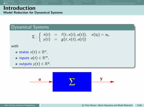
Dynamical Systems
Σ :
x(t) = f (t, x(t), u(t)), x(t0) = x0,y(t) = g(t, x(t), u(t))
with
states x(t) ∈ Rn,
inputs u(t) ∈ Rm,
outputs y(t) ∈ Rq.
Max Planck Institute Magdeburg c© Peter Benner, Matrix Equations and Model Reduction 5/96

Introduction Mathematical Basics MOR by Projection RatInt Balanced Truncation Matrix Equations Fin
Model Reduction for Dynamical Systems
Original System
Σ :
x(t) = f (t, x(t), u(t)),y(t) = g(t, x(t), u(t)).
states x(t) ∈ Rn,
inputs u(t) ∈ Rm,
outputs y(t) ∈ Rq.
Reduced-Order Model (ROM)
Σ :
˙x(t) = f (t, x(t), u(t)),y(t) = g(t, x(t), u(t)).
states x(t) ∈ Rr , r n
inputs u(t) ∈ Rm,
outputs y(t) ∈ Rq.
Goal:
‖y − y‖ < tolerance · ‖u‖ for all admissible input signals.
Max Planck Institute Magdeburg c© Peter Benner, Matrix Equations and Model Reduction 6/96

Introduction Mathematical Basics MOR by Projection RatInt Balanced Truncation Matrix Equations Fin
Model Reduction for Dynamical Systems
Original System
Σ :
x(t) = f (t, x(t), u(t)),y(t) = g(t, x(t), u(t)).
states x(t) ∈ Rn,
inputs u(t) ∈ Rm,
outputs y(t) ∈ Rq.
Reduced-Order Model (ROM)
Σ :
˙x(t) = f (t, x(t), u(t)),y(t) = g(t, x(t), u(t)).
states x(t) ∈ Rr , r n
inputs u(t) ∈ Rm,
outputs y(t) ∈ Rq.
Goal:
‖y − y‖ < tolerance · ‖u‖ for all admissible input signals.
Secondary goal: reconstruct approximation of x from x .
Max Planck Institute Magdeburg c© Peter Benner, Matrix Equations and Model Reduction 6/96

Introduction Mathematical Basics MOR by Projection RatInt Balanced Truncation Matrix Equations Fin
Model Reduction for Dynamical SystemsParameter-Dependent Dynamical Systems
Dynamical Systems
Σ(p) :
E (p)x(t; p) = f (t, x(t; p), u(t), p), x(t0) = x0, (a)
y(t; p) = g(t, x(t; p), u(t), p) (b)
with
(generalized) states x(t; p) ∈ Rn (E ∈ Rn×n),
inputs u(t) ∈ Rm,
outputs y(t; p) ∈ Rq, (b) is called output equation,
p ∈ Ω ⊂ Rd is a parameter vector, Ω is bounded.
Applications:
Repeated simulation for varying material or geometry parameters,boundary conditions,
Control, optimization and design.
Requirement: keep parameters as symbolic quantities in ROM.
Max Planck Institute Magdeburg c© Peter Benner, Matrix Equations and Model Reduction 7/96

Introduction Mathematical Basics MOR by Projection RatInt Balanced Truncation Matrix Equations Fin
Model Reduction for Dynamical SystemsLinear Systems
Linear, Time-Invariant (LTI) Systems
Ex = f (t, x , u) = Ax + Bu, E ,A ∈ Rn×n, B ∈ Rn×m,y = g(t, x , u) = Cx + Du, C ∈ Rq×n, D ∈ Rq×m.
Max Planck Institute Magdeburg c© Peter Benner, Matrix Equations and Model Reduction 8/96

Introduction Mathematical Basics MOR by Projection RatInt Balanced Truncation Matrix Equations Fin
Model Reduction for Dynamical SystemsLinear Systems
Linear, Time-Invariant (LTI) Systems
Ex = f (t, x , u) = Ax + Bu, E ,A ∈ Rn×n, B ∈ Rn×m,y = g(t, x , u) = Cx + Du, C ∈ Rq×n, D ∈ Rq×m.
Linear, Time-Invariant Parametric Systems
E (p)x(t; p) = A(p)x(t; p) + B(p)u(t),y(t; p) = C (p)x(t; p) + D(p)u(t),
where A(p),E (p) ∈ Rn×n,B(p) ∈ Rn×m,C (p) ∈ Rq×n,D(p) ∈ Rq×m.
Max Planck Institute Magdeburg c© Peter Benner, Matrix Equations and Model Reduction 8/96

Introduction Mathematical Basics MOR by Projection RatInt Balanced Truncation Matrix Equations Fin
Application AreasStructural Mechanics / Finite Element Modeling since ∼1960ies
Resolving complex 3D geometries ⇒ millions of degrees of freedom.
Analysis of elastic deformations requires many simulation runs forvarying external forces.
Standard MOR techniques in structural mechanics: modal truncation,combined with Guyan reduction (static condensation) Craig-Bamptonmethod.
Max Planck Institute Magdeburg c© Peter Benner, Matrix Equations and Model Reduction 9/96

Introduction Mathematical Basics MOR by Projection RatInt Balanced Truncation Matrix Equations Fin
Application Areas(Optimal) Control since ∼1980ies
Feedback Controllers
A feedback controller (dynamiccompensator) is a linear system oforder N, where
input = output of plant,
output = input of plant.
Modern (LQG-/H2-/H∞-) controldesign: N ≥ n.
Practical controllers require small N (N ∼ 10, say) due to– real-time constraints,
– increasing fragility for larger N.
=⇒ reduce order of plant (n) and/or controller (N).
Standard MOR techniques in systems and control: balanced truncationand related methods.
Max Planck Institute Magdeburg c© Peter Benner, Matrix Equations and Model Reduction 10/96

Introduction Mathematical Basics MOR by Projection RatInt Balanced Truncation Matrix Equations Fin
Application AreasMicro Electronics/Circuit Simulation since ∼1990ies
Progressive miniaturization
Verification of VLSI/ULSI chip design requires high number of simulationsfor different input signals.
Moore’s Law (1965/75) states that the number of on-chip transistorsdoubles each 24 months.
Source: http://en.wikipedia.org/wiki/File:Transistor_Count_and_Moore’sLaw_-_2011.svg
Max Planck Institute Magdeburg c© Peter Benner, Matrix Equations and Model Reduction 11/96

Introduction Mathematical Basics MOR by Projection RatInt Balanced Truncation Matrix Equations Fin
Application AreasMicro Electronics/Circuit Simulation since ∼1990ies
Progressive miniaturization
Verification of VLSI/ULSI chip design requires high number of simulationsfor different input signals.
Moore’s Law (1965/75) steady increase of describing equations, i.e.,network topology (Kirchhoff’s laws) and characteristic element/semi-conductor equations.
Increase in packing density and multilayer technology requires modeling ofinterconncet to ensure that thermic/electro-magnetic effects do notdisturb signal transmission.
Intel 4004 (1971) Intel Core 2 Extreme (quad-core) (2007)
1 layer, 10µ technology 9 layers, 45nm technology2,300 transistors > 8, 200, 000 transistors64 kHz clock speed > 3 GHz clock speed.
Max Planck Institute Magdeburg c© Peter Benner, Matrix Equations and Model Reduction 11/96

Introduction Mathematical Basics MOR by Projection RatInt Balanced Truncation Matrix Equations Fin
Application AreasMicro Electronics/Circuit Simulation since ∼1990ies
Progressive miniaturization
Verification of VLSI/ULSI chip design requires high number of simulationsfor different input signals.
Moore’s Law (1965/75) steady increase of describing equations, i.e.,network topology (Kirchhoff’s laws) and characteristic element/semi-conductor equations.
Increase in packing density and multilayer technology requires modeling ofinterconncet to ensure that thermic/electro-magnetic effects do notdisturb signal transmission.
Source: http://en.wikipedia.org/wiki/Image:Silicon_chip_3d.png.
Max Planck Institute Magdeburg c© Peter Benner, Matrix Equations and Model Reduction 11/96

Introduction Mathematical Basics MOR by Projection RatInt Balanced Truncation Matrix Equations Fin
Application AreasMicro Electronics/Circuit Simulation since ∼1990ies
Progressive miniaturization
Verification of VLSI/ULSI chip design requires high number of simulationsfor different input signals.
Moore’s Law (1965/75) steady increase of describing equations, i.e.,network topology (Kirchhoff’s laws) and characteristic element/semi-conductor equations.
Here: mostly MOR for linear systems, they occur in micro electronicsthrough modified nodal analysis (MNA) for RLC networks. e.g., when
decoupling large linear subcircuits,modeling transmission lines,modeling pin packages in VLSI chips,modeling circuit elements described by Maxwell’s equation usingpartial element equivalent circuits (PEEC).
Max Planck Institute Magdeburg c© Peter Benner, Matrix Equations and Model Reduction 11/96

Introduction Mathematical Basics MOR by Projection RatInt Balanced Truncation Matrix Equations Fin
Application AreasMicro Electronics/Circuit Simulation since ∼1990ies
Progressive miniaturization
Verification of VLSI/ULSI chip design requires high number of simulationsfor different input signals.
Moore’s Law (1965/75) steady increase of describing equations, i.e.,network topology (Kirchhoff’s laws) and characteristic element/semi-conductor equations.
Clear need for model reduction techniques in order to facilitate or evenenable circuit simulation for current and future VLSI design.
Standard MOR techniques in circuit simulation:Krylov subspace / Pade approximation / rational interpolation methods.
Max Planck Institute Magdeburg c© Peter Benner, Matrix Equations and Model Reduction 11/96
Introduction Mathematical Basics MOR by Projection RatInt Balanced Truncation Matrix Equations Fin
Application Areas
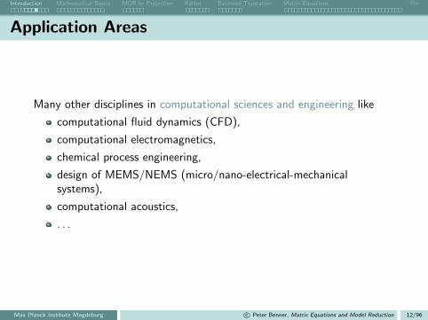
Many other disciplines in computational sciences and engineering like
computational fluid dynamics (CFD),
computational electromagnetics,
chemical process engineering,
design of MEMS/NEMS (micro/nano-electrical-mechanicalsystems),
computational acoustics,
. . .
Max Planck Institute Magdeburg c© Peter Benner, Matrix Equations and Model Reduction 12/96

Introduction Mathematical Basics MOR by Projection RatInt Balanced Truncation Matrix Equations Fin
Motivating ExamplesElectro-Thermic Simulation of Integrated Circuit (IC) [Source: Evgenii Rudnyi, CADFEM GmbH]
Simplorer R© test circuit with 2 transistors.
Conservative thermic sub-system in Simplorer:voltage temperature, current heat flow.
Original model: n = 270.593, m = q = 2 ⇒Computing time (on Intel Xeon dualcore 3GHz, 1 Thread):
– Main computational cost for set-up data ≈ 22min.– Computation of reduced models from set-up data: 44–49sec. (r = 20–70).– Bode plot (MATLAB on Intel Core i7, 2,67GHz, 12GB):
7.5h for original system, < 1min for reduced system.– Speed-up factor: 18 including / ≥ 450 excluding reduced model generation!
Max Planck Institute Magdeburg c© Peter Benner, Matrix Equations and Model Reduction 13/96

Introduction Mathematical Basics MOR by Projection RatInt Balanced Truncation Matrix Equations Fin
Motivating ExamplesElectro-Thermic Simulation of Integrated Circuit (IC) [Source: Evgenii Rudnyi, CADFEM GmbH]
Original model: n = 270.593, m = q = 2 ⇒Computing time (on Intel Xeon dualcore 3GHz, 1 Thread):
– Main computational cost for set-up data ≈ 22min.– Computation of reduced models from set-up data: 44–49sec. (r = 20–70).– Bode plot (MATLAB on Intel Core i7, 2,67GHz, 12GB):
7.5h for original system, < 1min for reduced system.– Speed-up factor: 18 including / ≥ 450 excluding reduced model generation!
Bode Plot (Amplitude)
10−2
100
102
104
10−1
100
101
102
ω
σm
ax(G
(jω
))
Transfer functions of original and reduced systems
original
ROM 20ROM 30
ROM 40
ROM 50ROM 60
ROM 70
Hankel Singular Values
50 100 150 200 250 300 350
10−20
10−15
10−10
10−5
100
Computed Hankel singular values
index
ma
gn
itu
de
Max Planck Institute Magdeburg c© Peter Benner, Matrix Equations and Model Reduction 13/96

Introduction Mathematical Basics MOR by Projection RatInt Balanced Truncation Matrix Equations Fin
Motivating ExamplesElectro-Thermic Simulation of Integrated Circuit (IC) [Source: Evgenii Rudnyi, CADFEM GmbH]
Original model: n = 270.593, m = q = 2 ⇒Computing time (on Intel Xeon dualcore 3GHz, 1 Thread):
– Main computational cost for set-up data ≈ 22min.– Computation of reduced models from set-up data: 44–49sec. (r = 20–70).– Bode plot (MATLAB on Intel Core i7, 2,67GHz, 12GB):
7.5h for original system, < 1min for reduced system.– Speed-up factor: 18 including / ≥ 450 excluding reduced model generation!
Absolute Error
10−2
100
102
104
10−8
10−7
10−6
10−5
10−4
10−3
10−2
10−1
absolute model reduction error
ω
σm
ax(G
(jω
) −
Gr(j
ω))
ROM 20
ROM 30
ROM 40
ROM 50
ROM 60
ROM 70
Relative Error
10−2
100
102
104
10−9
10−7
10−5
10−3
10−1
relative model reduction error
ω
σm
ax(G
(jω
) −
Gr(j
ω))
/ ||G
||∞
ROM 20
ROM 30
ROM 40
ROM 50
ROM 60
ROM 70
Max Planck Institute Magdeburg c© Peter Benner, Matrix Equations and Model Reduction 13/96
Introduction Mathematical Basics MOR by Projection RatInt Balanced Truncation Matrix Equations Fin
Motivating ExamplesA Nonlinear Model from Computational Neurosciences: the FitzHugh-Nagumo System
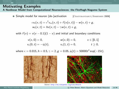
Simple model for neuron (de-)activation [Chaturantabut/Sorensen 2009]
εvt(x , t) = ε2vxx(x , t) + f (v(x , t))− w(x , t) + g ,
wt(x , t) = hv(x , t)− γw(x , t) + g ,
with f (v) = v(v − 0.1)(1− v) and initial and boundary conditions
v(x , 0) = 0, w(x , 0) = 0, x ∈ [0, 1]
vx(0, t) = −i0(t), vx(1, t) = 0, t ≥ 0,
where ε = 0.015, h = 0.5, γ = 2, g = 0.05, i0(t) = 50000t3 exp(−15t).
Source: http://en.wikipedia.org/wiki/Neuron
Max Planck Institute Magdeburg c© Peter Benner, Matrix Equations and Model Reduction 14/96

Introduction Mathematical Basics MOR by Projection RatInt Balanced Truncation Matrix Equations Fin
Motivating ExamplesA Nonlinear Model from Computational Neurosciences: the FitzHugh-Nagumo System
Simple model for neuron (de-)activation [Chaturantabut/Sorensen 2009]
εvt(x , t) = ε2vxx(x , t) + f (v(x , t))− w(x , t) + g ,
wt(x , t) = hv(x , t)− γw(x , t) + g ,
with f (v) = v(v − 0.1)(1− v) and initial and boundary conditions
v(x , 0) = 0, w(x , 0) = 0, x ∈ [0, 1]
vx(0, t) = −i0(t), vx(1, t) = 0, t ≥ 0,
where ε = 0.015, h = 0.5, γ = 2, g = 0.05, i0(t) = 50000t3 exp(−15t).
Parameter g handled as an additional input.
Original state dimension n = 2 · 400, QBDAE dimension N = 3 · 400,reduced QBDAE dimension r = 26, chosen expansion point σ = 1.
Max Planck Institute Magdeburg c© Peter Benner, Matrix Equations and Model Reduction 14/96

Introduction Mathematical Basics MOR by Projection RatInt Balanced Truncation Matrix Equations Fin
Motivating ExamplesA Nonlinear Model from Computational Neurosciences: the FitzHugh-Nagumo System
Max Planck Institute Magdeburg c© Peter Benner, Matrix Equations and Model Reduction 14/96

Introduction Mathematical Basics MOR by Projection RatInt Balanced Truncation Matrix Equations Fin
Motivating ExamplesParametric MOR: Applications in Microsystems/MEMS Design
Microgyroscope (butterfly gyro)
Voltage applied to electrodes inducesvibration of wings, resulting rotation dueto Coriolis force yields sensor data.
FE model of second order:N = 17.361 n = 34.722, m = 1, q = 12.
Sensor for position control based onacceleration and rotation.
Application: inertial navigation.
Source: The Oberwolfach Benchmark Collection http://www.imtek.de/simulation/benchmark
Max Planck Institute Magdeburg c© Peter Benner, Matrix Equations and Model Reduction 15/96
Introduction Mathematical Basics MOR by Projection RatInt Balanced Truncation Matrix Equations Fin
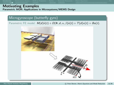
Motivating ExamplesParametric MOR: Applications in Microsystems/MEMS Design
Microgyroscope (butterfly gyro)
Parametric FE model: M(d)x(t) + D(Φ, d , α, β)x(t) + T (d)x(t) = Bu(t).
Max Planck Institute Magdeburg c© Peter Benner, Matrix Equations and Model Reduction 15/96

Introduction Mathematical Basics MOR by Projection RatInt Balanced Truncation Matrix Equations Fin
Motivating ExamplesParametric MOR: Applications in Microsystems/MEMS Design
Microgyroscope (butterfly gyro)
Parametric FE model:
M(d)x(t) + D(Φ, d , α, β)x(t) + T (d)x(t) = Bu(t),
wobei
M(d) = M1 + dM2,
D(Φ, d , α, β) = Φ(D1 + dD2) + αM(d) + βT (d),
T (d) = T1 +1
dT2 + dT3,
with
width of bearing: d ,
angular velocity: Φ,
Rayleigh damping parameters: α, β.
Max Planck Institute Magdeburg c© Peter Benner, Matrix Equations and Model Reduction 15/96

Introduction Mathematical Basics MOR by Projection RatInt Balanced Truncation Matrix Equations Fin
Motivating ExamplesParametric MOR: Applications in Microsystems/MEMS Design
Microgyroscope (butterfly gyro)
Original. . . and reduced-order model.
Max Planck Institute Magdeburg c© Peter Benner, Matrix Equations and Model Reduction 15/96

Introduction Mathematical Basics MOR by Projection RatInt Balanced Truncation Matrix Equations Fin
Outline
1 Introduction
2 Mathematical BasicsNumerical Linear AlgebraSystems and Control TheoryQualitative and Quantitative Study of the Approximation Error
3 Model Reduction by Projection
4 Interpolatory Model Reduction
5 Balanced Truncation
6 Solving Large-Scale Matrix Equations
7 Final Remarks
Max Planck Institute Magdeburg c© Peter Benner, Matrix Equations and Model Reduction 16/96

Introduction Mathematical Basics MOR by Projection RatInt Balanced Truncation Matrix Equations Fin
Numerical Linear AlgebraImage Compression by Truncated SVD
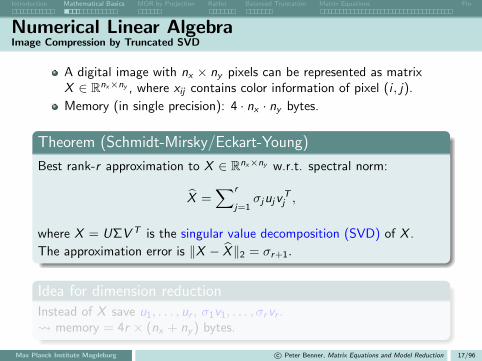
A digital image with nx × ny pixels can be represented as matrixX ∈ Rnx×ny , where xij contains color information of pixel (i , j).
Memory (in single precision): 4 · nx · ny bytes.
Theorem (Schmidt-Mirsky/Eckart-Young)
Best rank-r approximation to X ∈ Rnx×ny w.r.t. spectral norm:
X =∑r
j=1σjujv
Tj ,
where X = UΣV T is the singular value decomposition (SVD) of X .
The approximation error is ‖X − X‖2 = σr+1.
Idea for dimension reductionInstead of X save u1, . . . , ur , σ1v1, . . . , σrvr . memory = 4r × (nx + ny ) bytes.
Max Planck Institute Magdeburg c© Peter Benner, Matrix Equations and Model Reduction 17/96
Introduction Mathematical Basics MOR by Projection RatInt Balanced Truncation Matrix Equations Fin
Numerical Linear AlgebraImage Compression by Truncated SVD
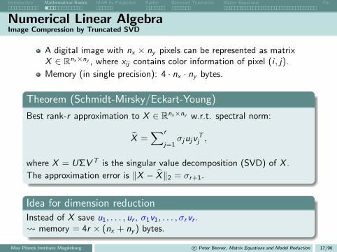
A digital image with nx × ny pixels can be represented as matrixX ∈ Rnx×ny , where xij contains color information of pixel (i , j).
Memory (in single precision): 4 · nx · ny bytes.
Theorem (Schmidt-Mirsky/Eckart-Young)
Best rank-r approximation to X ∈ Rnx×ny w.r.t. spectral norm:
X =∑r
j=1σjujv
Tj ,
where X = UΣV T is the singular value decomposition (SVD) of X .
The approximation error is ‖X − X‖2 = σr+1.
Idea for dimension reductionInstead of X save u1, . . . , ur , σ1v1, . . . , σrvr . memory = 4r × (nx + ny ) bytes.
Max Planck Institute Magdeburg c© Peter Benner, Matrix Equations and Model Reduction 17/96
Introduction Mathematical Basics MOR by Projection RatInt Balanced Truncation Matrix Equations Fin
Numerical Linear AlgebraImage Compression by Truncated SVD
A digital image with nx × ny pixels can be represented as matrixX ∈ Rnx×ny , where xij contains color information of pixel (i , j).
Memory (in single precision): 4 · nx · ny bytes.
Theorem (Schmidt-Mirsky/Eckart-Young)
Best rank-r approximation to X ∈ Rnx×ny w.r.t. spectral norm:
X =∑r
j=1σjujv
Tj ,
where X = UΣV T is the singular value decomposition (SVD) of X .
The approximation error is ‖X − X‖2 = σr+1.
Idea for dimension reductionInstead of X save u1, . . . , ur , σ1v1, . . . , σrvr . memory = 4r × (nx + ny ) bytes.
Max Planck Institute Magdeburg c© Peter Benner, Matrix Equations and Model Reduction 17/96

Introduction Mathematical Basics MOR by Projection RatInt Balanced Truncation Matrix Equations Fin
Example: Image Compression by Truncated SVD
Example: Clown
320× 200 pixel ≈ 256 kB
rank r = 50, ≈ 104 kB
rank r = 20, ≈ 42 kB
Max Planck Institute Magdeburg c© Peter Benner, Matrix Equations and Model Reduction 18/96

Introduction Mathematical Basics MOR by Projection RatInt Balanced Truncation Matrix Equations Fin
Dimension Reduction via SVD
Example: GatlinburgOrganizing committeeGatlinburg/Householder Meeting 1964:
James H. Wilkinson, Wallace Givens,
George Forsythe, Alston Householder,
Peter Henrici, Fritz L. Bauer.
640× 480 pixel, ≈ 1229 kB
Max Planck Institute Magdeburg c© Peter Benner, Matrix Equations and Model Reduction 19/96

Introduction Mathematical Basics MOR by Projection RatInt Balanced Truncation Matrix Equations Fin
Dimension Reduction via SVD
Example: GatlinburgOrganizing committeeGatlinburg/Householder Meeting 1964:
James H. Wilkinson, Wallace Givens,
George Forsythe, Alston Householder,
Peter Henrici, Fritz L. Bauer.
640× 480 pixel, ≈ 1229 kB
rank r = 100, ≈ 448 kB
rank r = 50, ≈ 224 kB
Max Planck Institute Magdeburg c© Peter Benner, Matrix Equations and Model Reduction 19/96

Introduction Mathematical Basics MOR by Projection RatInt Balanced Truncation Matrix Equations Fin
Background: Singular Value Decay
Image data compression via SVD works, if the singular values decay(exponentially).
Singular Values of the Image Data Matrices
Max Planck Institute Magdeburg c© Peter Benner, Matrix Equations and Model Reduction 20/96

Introduction Mathematical Basics MOR by Projection RatInt Balanced Truncation Matrix Equations Fin
Systems and Control TheoryThe Laplace transform
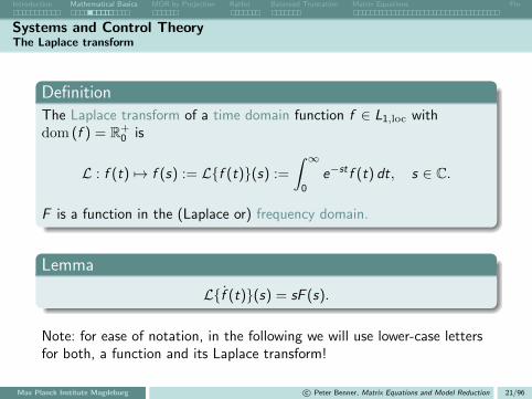
DefinitionThe Laplace transform of a time domain function f ∈ L1,loc withdom (f ) = R+
0 is
L : f (t) 7→ f (s) := Lf (t)(s) :=
∫ ∞0
e−st f (t) dt, s ∈ C.
F is a function in the (Laplace or) frequency domain.
Note: for frequency domain evaluations (”frequency response analysis”), onetakes re s = 0 and im s ≥ 0. Then ω := im s takes the role of a frequency (in[rad/s], i.e., ω = 2πv with v measured in [Hz]).
Max Planck Institute Magdeburg c© Peter Benner, Matrix Equations and Model Reduction 21/96

Introduction Mathematical Basics MOR by Projection RatInt Balanced Truncation Matrix Equations Fin
Systems and Control TheoryThe Laplace transform
DefinitionThe Laplace transform of a time domain function f ∈ L1,loc withdom (f ) = R+
0 is
L : f (t) 7→ f (s) := Lf (t)(s) :=
∫ ∞0
e−st f (t) dt, s ∈ C.
F is a function in the (Laplace or) frequency domain.
Note: for frequency domain evaluations (”frequency response analysis”), onetakes re s = 0 and im s ≥ 0. Then ω := im s takes the role of a frequency (in[rad/s], i.e., ω = 2πv with v measured in [Hz]).
Lemma
Lf (t)(s) = sF (s).
Max Planck Institute Magdeburg c© Peter Benner, Matrix Equations and Model Reduction 21/96
Introduction Mathematical Basics MOR by Projection RatInt Balanced Truncation Matrix Equations Fin
Systems and Control TheoryThe Laplace transform
DefinitionThe Laplace transform of a time domain function f ∈ L1,loc withdom (f ) = R+
0 is
L : f (t) 7→ f (s) := Lf (t)(s) :=
∫ ∞0
e−st f (t) dt, s ∈ C.
F is a function in the (Laplace or) frequency domain.
Lemma
Lf (t)(s) = sF (s).
Note: for ease of notation, in the following we will use lower-case lettersfor both, a function and its Laplace transform!
Max Planck Institute Magdeburg c© Peter Benner, Matrix Equations and Model Reduction 21/96

Introduction Mathematical Basics MOR by Projection RatInt Balanced Truncation Matrix Equations Fin
Systems and Control TheoryThe Model Reduction Problem as Approximation Problem in Frequency Domain
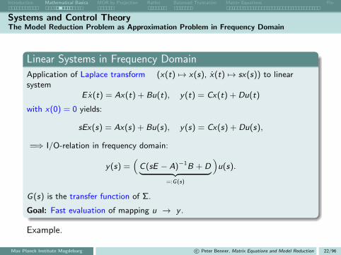
Linear Systems in Frequency Domain
Application of Laplace transform (x(t) 7→ x(s), x(t) 7→ sx(s)) to linearsystem
Ex(t) = Ax(t) + Bu(t), y(t) = Cx(t) + Du(t)
with x(0) = 0 yields:
sEx(s) = Ax(s) + Bu(s), y(s) = Cx(s) + Du(s),
Max Planck Institute Magdeburg c© Peter Benner, Matrix Equations and Model Reduction 22/96

Introduction Mathematical Basics MOR by Projection RatInt Balanced Truncation Matrix Equations Fin
Systems and Control TheoryThe Model Reduction Problem as Approximation Problem in Frequency Domain
Linear Systems in Frequency Domain
Application of Laplace transform (x(t) 7→ x(s), x(t) 7→ sx(s)) to linearsystem
Ex(t) = Ax(t) + Bu(t), y(t) = Cx(t) + Du(t)
with x(0) = 0 yields:
sEx(s) = Ax(s) + Bu(s), y(s) = Cx(s) + Du(s),
=⇒ I/O-relation in frequency domain:
y(s) =(C(sE − A)−1B + D︸ ︷︷ ︸
=:G(s)
)u(s).
G(s) is the transfer function of Σ.
Goal: Fast evaluation of mapping u → y .
Max Planck Institute Magdeburg c© Peter Benner, Matrix Equations and Model Reduction 22/96
Introduction Mathematical Basics MOR by Projection RatInt Balanced Truncation Matrix Equations Fin
Systems and Control TheoryThe Model Reduction Problem as Approximation Problem in Frequency Domain
Linear Systems in Frequency Domain
Application of Laplace transform (x(t) 7→ x(s), x(t) 7→ sx(s)) to linearsystem
Ex(t) = Ax(t) + Bu(t), y(t) = Cx(t) + Du(t)
with x(0) = 0 yields:
sEx(s) = Ax(s) + Bu(s), y(s) = Cx(s) + Du(s),
=⇒ I/O-relation in frequency domain:
y(s) =(C(sE − A)−1B + D︸ ︷︷ ︸
=:G(s)
)u(s).
G(s) is the transfer function of Σ.
Goal: Fast evaluation of mapping u → y .
Example.
Max Planck Institute Magdeburg c© Peter Benner, Matrix Equations and Model Reduction 22/96

Introduction Mathematical Basics MOR by Projection RatInt Balanced Truncation Matrix Equations Fin
Systems and Control TheoryThe Model Reduction Problem as Approximation Problem in Frequency Domain
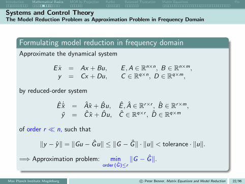
Formulating model reduction in frequency domain
Approximate the dynamical system
Ex = Ax + Bu, E ,A ∈ Rn×n, B ∈ Rn×m,y = Cx + Du, C ∈ Rq×n, D ∈ Rq×m,
by reduced-order system
E ˙x = Ax + Bu, E , A ∈ Rr×r , B ∈ Rr×m,
y = C x + Du, C ∈ Rq×r , D ∈ Rq×m
of order r n, such that
‖y − y‖ = ‖Gu − Gu‖ ≤ ‖G − G‖ · ‖u‖ < tolerance · ‖u‖.
Max Planck Institute Magdeburg c© Peter Benner, Matrix Equations and Model Reduction 22/96
Introduction Mathematical Basics MOR by Projection RatInt Balanced Truncation Matrix Equations Fin
Systems and Control TheoryThe Model Reduction Problem as Approximation Problem in Frequency Domain
Formulating model reduction in frequency domain
Approximate the dynamical system
Ex = Ax + Bu, E ,A ∈ Rn×n, B ∈ Rn×m,y = Cx + Du, C ∈ Rq×n, D ∈ Rq×m,
by reduced-order system
E ˙x = Ax + Bu, E , A ∈ Rr×r , B ∈ Rr×m,
y = C x + Du, C ∈ Rq×r , D ∈ Rq×m
of order r n, such that
‖y − y‖ = ‖Gu − Gu‖ ≤ ‖G − G‖ · ‖u‖ < tolerance · ‖u‖.
=⇒ Approximation problem: minorder (G)≤r
‖G − G‖.
Max Planck Institute Magdeburg c© Peter Benner, Matrix Equations and Model Reduction 22/96

Introduction Mathematical Basics MOR by Projection RatInt Balanced Truncation Matrix Equations Fin
Systems and Control TheoryProperties of linear systems
DefinitionA linear system
Ex(t) = Ax(t) + Bu(t), y(t) = Cx(t) + Du(t)
is stable if its transfer function G (s) has all its poles in the left half planeand it is asymptotically (or Lyapunov or exponentially) stable if all polesare in the open left half plane C− := z ∈ C | <(z) < 0.
Lemma
Sufficient for asymptotic stability is that A is asymptotically stable (orHurwitz), i.e., the spectrum of A− λE , denoted by Λ (A,E ), satisfiesΛ (A,E ) ⊂ C−.
Note that by abuse of notation, often stable system is used for asymptotically
stable systems.
Max Planck Institute Magdeburg c© Peter Benner, Matrix Equations and Model Reduction 23/96

Introduction Mathematical Basics MOR by Projection RatInt Balanced Truncation Matrix Equations Fin
Systems and Control TheoryProperties of linear systems
Further properties to be discussed:
Controllability/reachability
Observability
Stabilizability
Detectability
See handout ”Mathematical Basics”.
Max Planck Institute Magdeburg c© Peter Benner, Matrix Equations and Model Reduction 24/96
Introduction Mathematical Basics MOR by Projection RatInt Balanced Truncation Matrix Equations Fin
Systems and Control TheoryRealizations of Linear Systems (with E = In for simplicity)
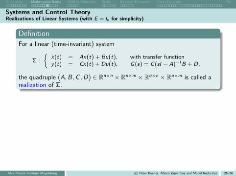
Definition
For a linear (time-invariant) system
Σ :
x(t) = Ax(t) + Bu(t), with transfer functiony(t) = Cx(t) + Du(t), G(s) = C(sI − A)−1B + D,
the quadruple (A,B,C ,D) ∈ Rn×n × Rn×m × Rq×n × Rq×m is called arealization of Σ.
Max Planck Institute Magdeburg c© Peter Benner, Matrix Equations and Model Reduction 25/96

Introduction Mathematical Basics MOR by Projection RatInt Balanced Truncation Matrix Equations Fin
Systems and Control TheoryRealizations of Linear Systems (with E = In for simplicity)
Definition
For a linear (time-invariant) system
Σ :
x(t) = Ax(t) + Bu(t), with transfer functiony(t) = Cx(t) + Du(t), G(s) = C(sI − A)−1B + D,
the quadruple (A,B,C ,D) ∈ Rn×n × Rn×m × Rq×n × Rq×m is called arealization of Σ.
Realizations are not unique!Transfer function is invariant under state-space transformations,
T :
x → Tx ,
(A,B,C ,D) → (TAT−1,TB,CT−1,D),
Max Planck Institute Magdeburg c© Peter Benner, Matrix Equations and Model Reduction 25/96

Introduction Mathematical Basics MOR by Projection RatInt Balanced Truncation Matrix Equations Fin
Systems and Control TheoryRealizations of Linear Systems (with E = In for simplicity)
Definition
For a linear (time-invariant) system
Σ :
x(t) = Ax(t) + Bu(t), with transfer functiony(t) = Cx(t) + Du(t), G(s) = C(sI − A)−1B + D,
the quadruple (A,B,C ,D) ∈ Rn×n × Rn×m × Rq×n × Rq×m is called arealization of Σ.
Realizations are not unique!
Transfer function is invariant under addition of uncontrollable/unobservablestates:
d
dt
[xx1
]=
[A 0
0 A1
] [xx1
]+
[BB1
]u(t), y(t) =
[C 0
] [ xx1
]+ Du(t),
d
dt
[xx2
]=
[A 0
0 A2
] [xx2
]+
[B0
]u(t), y(t) =
[C C2
] [ xx2
]+ Du(t),
for arbitrary Aj ∈ Rnj×nj , j = 1, 2, B1 ∈ Rn1×m, C2 ∈ Rq×n2 and any n1, n2 ∈ N.
Max Planck Institute Magdeburg c© Peter Benner, Matrix Equations and Model Reduction 25/96

Introduction Mathematical Basics MOR by Projection RatInt Balanced Truncation Matrix Equations Fin
Systems and Control TheoryRealizations of Linear Systems (with E = In for simplicity)
Definition
For a linear (time-invariant) system
Σ :
x(t) = Ax(t) + Bu(t), with transfer functiony(t) = Cx(t) + Du(t), G(s) = C(sI − A)−1B + D,
the quadruple (A,B,C ,D) ∈ Rn×n × Rn×m × Rq×n × Rq×m is called arealization of Σ.
Realizations are not unique!Hence,
(A,B,C ,D),
([A 0
0 A1
],
[BB1
],[C 0
],D
),
(TAT−1,TB,CT−1,D),
([A 0
0 A2
],
[B0
],[C C2
],D
),
are all realizations of Σ!
Max Planck Institute Magdeburg c© Peter Benner, Matrix Equations and Model Reduction 25/96

Introduction Mathematical Basics MOR by Projection RatInt Balanced Truncation Matrix Equations Fin
Systems and Control TheoryRealizations of Linear Systems (with E = In for simplicity)
Definition
For a linear (time-invariant) system
Σ :
x(t) = Ax(t) + Bu(t), with transfer functiony(t) = Cx(t) + Du(t), G(s) = C(sI − A)−1B + D,
the quadruple (A,B,C ,D) ∈ Rn×n × Rn×m × Rq×n × Rq×m is called arealization of Σ.
DefinitionThe McMillan degree of Σ is the unique minimal number n ≥ 0 of statesnecessary to describe the input-output behavior completely.A minimal realization is a realization (A, B, C , D) of Σ with order n.
Theorem
A realization (A,B,C ,D) of a linear system is minimal ⇐⇒(A,B) is controllable and (A,C ) is observable.
Max Planck Institute Magdeburg c© Peter Benner, Matrix Equations and Model Reduction 25/96

Introduction Mathematical Basics MOR by Projection RatInt Balanced Truncation Matrix Equations Fin
Systems and Control TheoryBalanced Realizations
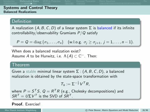
Definition
A realization (A,B,C ,D) of a linear system Σ is balanced if its infinitecontrollability/observability Gramians P/Q satisfy
P = Q = diag σ1, . . . , σn (w.l.o.g. σj ≥ σj+1, j = 1, . . . , n − 1).
Max Planck Institute Magdeburg c© Peter Benner, Matrix Equations and Model Reduction 26/96

Introduction Mathematical Basics MOR by Projection RatInt Balanced Truncation Matrix Equations Fin
Systems and Control TheoryBalanced Realizations
Definition
A realization (A,B,C ,D) of a linear system Σ is balanced if its infinitecontrollability/observability Gramians P/Q satisfy
P = Q = diag σ1, . . . , σn (w.l.o.g. σj ≥ σj+1, j = 1, . . . , n − 1).
When does a balanced realization exist?
Max Planck Institute Magdeburg c© Peter Benner, Matrix Equations and Model Reduction 26/96
Introduction Mathematical Basics MOR by Projection RatInt Balanced Truncation Matrix Equations Fin
Systems and Control TheoryBalanced Realizations
Definition
A realization (A,B,C ,D) of a linear system Σ is balanced if its infinitecontrollability/observability Gramians P/Q satisfy
P = Q = diag σ1, . . . , σn (w.l.o.g. σj ≥ σj+1, j = 1, . . . , n − 1).
When does a balanced realization exist?Assume A to be Hurwitz, i.e. Λ (A) ⊂ C−. Then:
Theorem
Given a stable minimal linear system Σ : (A,B,C ,D), a balancedrealization is obtained by the state-space transformation with
Tb := Σ−12 V TR,
where P = STS , Q = RTR (e.g., Cholesky decompositions) andSRT = UΣV T is the SVD of SRT .
Proof. Exercise!
Max Planck Institute Magdeburg c© Peter Benner, Matrix Equations and Model Reduction 26/96

Introduction Mathematical Basics MOR by Projection RatInt Balanced Truncation Matrix Equations Fin
Systems and Control TheoryBalanced Realizations
Definition
A realization (A,B,C ,D) of a stable linear system Σ is balanced if itsinfinite controllability/observability Gramians P/Q satisfy
P = Q = diag σ1, . . . , σn (w.l.o.g. σj ≥ σj+1, j = 1, . . . , n − 1).
σ1, . . . , σn are the Hankel singular values of Σ.
Note: σ1, . . . , σn ≥ 0 as P,Q ≥ 0 by definition, and σ1, . . . , σn > 0 in case ofminimality!
TheoremThe infinite controllability/observability Gramians P/Q satisfy the Lyapunovequations
AP + PAT + BBT = 0, ATQ + QA + CTC = 0.
Max Planck Institute Magdeburg c© Peter Benner, Matrix Equations and Model Reduction 26/96

Introduction Mathematical Basics MOR by Projection RatInt Balanced Truncation Matrix Equations Fin
Systems and Control TheoryBalanced Realizations
Theorem
The infinite controllability/observability Gramians P/Q satisfy theLyapunov equations
AP + PAT + BBT = 0, ATQ + QA + CTC = 0.
Proof. (For controllability Gramian only, observability case is analogous!)
AP + PAT + BBT = A
∫ ∞0
eAtBBT eATtdt +
∫ ∞0
eAtBBT eATtdt AT + BBT
=
∫ ∞0
AeAtBBT eATt + eAtBBT eA
TtAT︸ ︷︷ ︸= d
dteAtBBT eA
Tt
dt + BBT
= limt→∞
eAtBBT eATt︸ ︷︷ ︸
= 0
− eA·0︸︷︷︸= In
BBT eAT ·0︸ ︷︷ ︸
= In
+BBT
= 0.
Max Planck Institute Magdeburg c© Peter Benner, Matrix Equations and Model Reduction 26/96

Introduction Mathematical Basics MOR by Projection RatInt Balanced Truncation Matrix Equations Fin
Systems and Control TheoryBalanced Realizations
Definition
A realization (A,B,C ,D) of a stable linear system Σ is balanced if itsinfinite controllability/observability Gramians P/Q satisfy
P = Q = diag σ1, . . . , σn (w.l.o.g. σj ≥ σj+1, j = 1, . . . , n − 1).
σ1, . . . , σn are the Hankel singular values of Σ.
Note: σ1, . . . , σn ≥ 0 as P,Q ≥ 0 by definition, and σ1, . . . , σn > 0 in case ofminimality!
TheoremThe Hankel singular values (HSVs) of a stable minimal linear system are systeminvariants, i.e. they are unaltered by state-space transformations!
Max Planck Institute Magdeburg c© Peter Benner, Matrix Equations and Model Reduction 26/96

Introduction Mathematical Basics MOR by Projection RatInt Balanced Truncation Matrix Equations Fin
Systems and Control TheoryBalanced Realizations
Theorem
The Hankel singular values (HSVs) of a stable minimal linear system aresystem invariants, i.e. they are unaltered by state-space transformations!
Proof. In balanced coordinates, the HSVs are Λ (PQ)12 . Now let
(A, B, C ,D) = (TAT−1,TB,CT−1,D)
be any transformed realization with associated controllability Lyapunov equation
0 = AP + PAT + BBT = TAT−1P + PT−TATTT + TBBTTT .
This is equivalent to
0 = A(T−1PT−T ) + (T−1PT−T )AT + BBT .
The uniqueness of the solution of the Lyapunov equation implies that P = TPTT and,analogously, Q = T−TQT−1. Therefore,
PQ = TPQT−1,
showing that Λ (PQ) = Λ (PQ) = σ21 , . . . , σ
2n.
Max Planck Institute Magdeburg c© Peter Benner, Matrix Equations and Model Reduction 26/96

Introduction Mathematical Basics MOR by Projection RatInt Balanced Truncation Matrix Equations Fin
Systems and Control TheoryBalanced Realizations
Definition
A realization (A,B,C ,D) of a stable linear system Σ is balanced if itsinfinite controllability/observability Gramians P/Q satisfy
P = Q = diag σ1, . . . , σn (w.l.o.g. σj ≥ σj+1, j = 1, . . . , n − 1).
σ1, . . . , σn are the Hankel singular values of Σ.
Note: σ1, . . . , σn ≥ 0 as P,Q ≥ 0 by definition, and σ1, . . . , σn > 0 in case ofminimality!
RemarkFor non-minimal systems, the Gramians can also be transformed into diagonalmatrices with the leading n × n submatrices equal to diag(σ1, . . . , σn), and
PQ = diag(σ21 , . . . , σ
2n, 0, . . . , 0).
see [Laub/Heath/Paige/Ward 1987, Tombs/Postlethwaite 1987].
Max Planck Institute Magdeburg c© Peter Benner, Matrix Equations and Model Reduction 26/96

Introduction Mathematical Basics MOR by Projection RatInt Balanced Truncation Matrix Equations Fin
Qualitative and Quantitative Study of the Approximation ErrorSystem Norms
Consider transfer function
G (s) = C (sI − A)−1 B + D
and input functions u ∈ Lm2∼= Lm2 (−∞,∞), with the L2-norm
‖u‖22 :=
1
2π
∫ ∞−∞
u(ω)Hu(ω) dω.
Assume A (asympotically) stable: Λ (A) ⊂ C− := z ∈ C : re z < 0.
Max Planck Institute Magdeburg c© Peter Benner, Matrix Equations and Model Reduction 27/96
Introduction Mathematical Basics MOR by Projection RatInt Balanced Truncation Matrix Equations Fin
Qualitative and Quantitative Study of the Approximation ErrorSystem Norms
Consider transfer function
G (s) = C (sI − A)−1 B + D
and input functions u ∈ Lm2∼= Lm2 (−∞,∞), with the L2-norm
‖u‖22 :=
1
2π
∫ ∞−∞
u(ω)Hu(ω) dω.
Assume A (asympotically) stable: Λ (A) ⊂ C− := z ∈ C : re z < 0.Then for all s ∈ C+ ∪ R, ‖G (s)‖ ≤ M <∞ ⇒∫ ∞
−∞y(ω)Hy(ω) dω =
∫ ∞−∞
u(ω)HG(ω)HG(ω)u(ω) dω
(Here, ‖ . ‖ denotes the Euclidian vector or spectral matrix norm.)
Max Planck Institute Magdeburg c© Peter Benner, Matrix Equations and Model Reduction 27/96

Introduction Mathematical Basics MOR by Projection RatInt Balanced Truncation Matrix Equations Fin
Qualitative and Quantitative Study of the Approximation ErrorSystem Norms
Consider transfer function
G (s) = C (sI − A)−1 B + D
and input functions u ∈ Lm2∼= Lm2 (−∞,∞), with the L2-norm
‖u‖22 :=
1
2π
∫ ∞−∞
u(ω)Hu(ω) dω.
Assume A (asympotically) stable: Λ (A) ⊂ C− := z ∈ C : re z < 0.Then for all s ∈ C+ ∪ R, ‖G (s)‖ ≤ M <∞ ⇒∫ ∞
−∞y(ω)Hy(ω) dω =
∫ ∞−∞
u(ω)HG(ω)HG(ω)u(ω) dω
=
∫ ∞−∞‖G(ω)u(ω)‖2 dω ≤
∫ ∞−∞
M2‖u(ω)‖2 dω
= M2∫ ∞−∞
u(ω)Hu(ω) dω < ∞.
(Here, ‖ . ‖ denotes the Euclidian vector or spectral matrix norm.)
Max Planck Institute Magdeburg c© Peter Benner, Matrix Equations and Model Reduction 27/96
Introduction Mathematical Basics MOR by Projection RatInt Balanced Truncation Matrix Equations Fin
Qualitative and Quantitative Study of the Approximation ErrorSystem Norms
Consider transfer function
G (s) = C (sI − A)−1 B + D
and input functions u ∈ Lm2∼= Lm2 (−∞,∞), with the L2-norm
‖u‖22 :=
1
2π
∫ ∞−∞
u(ω)Hu(ω) dω.
Assume A (asympotically) stable: Λ (A) ⊂ C− := z ∈ C : re z < 0.Then for all s ∈ C+ ∪ R, ‖G (s)‖ ≤ M <∞ ⇒∫ ∞
−∞y(ω)Hy(ω) dω =
∫ ∞−∞
u(ω)HG(ω)HG(ω)u(ω) dω
=
∫ ∞−∞‖G(ω)u(ω)‖2 dω ≤
∫ ∞−∞
M2‖u(ω)‖2 dω
= M2∫ ∞−∞
u(ω)Hu(ω) dω < ∞.
=⇒ y ∈ Lq2∼= Lq2(−∞,∞).
Max Planck Institute Magdeburg c© Peter Benner, Matrix Equations and Model Reduction 27/96

Introduction Mathematical Basics MOR by Projection RatInt Balanced Truncation Matrix Equations Fin
Qualitative and Quantitative Study of the Approximation ErrorSystem Norms
Consider transfer function
G (s) = C (sI − A)−1 B + D
and input functions u ∈ Lm2∼= Lm2 (−∞,∞), with the L2-norm
‖u‖22 :=
1
2π
∫ ∞−∞
u(ω)Hu(ω) dω.
Assume A (asympotically) stable: Λ (A) ⊂ C− := z ∈ C : re z < 0.Consequently, the 2-induced operator norm
‖G‖∞ := sup‖u‖2 6=0
‖Gu‖2
‖u‖2
is well defined. It can be shown that
‖G‖∞ = supω∈R‖G (ω)‖ = sup
ω∈Rσmax (G (ω)) .
Max Planck Institute Magdeburg c© Peter Benner, Matrix Equations and Model Reduction 27/96
Introduction Mathematical Basics MOR by Projection RatInt Balanced Truncation Matrix Equations Fin
Qualitative and Quantitative Study of the Approximation ErrorSystem Norms
Consider transfer function
G (s) = C (sI − A)−1 B + D
and input functions u ∈ Lm2∼= Lm2 (−∞,∞), with the L2-norm
‖u‖22 :=
1
2π
∫ ∞−∞
u(ω)Hu(ω) dω.
Assume A (asympotically) stable: Λ (A) ⊂ C− := z ∈ C : re z < 0.Consequently, the 2-induced operator norm
‖G‖∞ := sup‖u‖2 6=0
‖Gu‖2
‖u‖2
is well defined. It can be shown that
‖G‖∞ = supω∈R‖G (ω)‖ = sup
ω∈Rσmax (G (ω)) .
Sketch of proof:
‖G(ω)u(ω)‖ ≤ ‖G(ω)‖‖u(ω)‖ ⇒ ”≤”.Construct u with ‖Gu‖2 = supω∈R ‖G(ω)‖‖u‖2.
Max Planck Institute Magdeburg c© Peter Benner, Matrix Equations and Model Reduction 27/96

Introduction Mathematical Basics MOR by Projection RatInt Balanced Truncation Matrix Equations Fin
Qualitative and Quantitative Study of the Approximation ErrorSystem Norms
Consider transfer function
G (s) = C (sI − A)−1 B + D.
Hardy space H∞Function space of matrix-/scalar-valued functions that are analytic andbounded in C+.The H∞-norm is
‖F‖∞ := supre s>0
σmax (F (s)) = supω∈R
σmax (F (ω)) .
Stable transfer functions are in the Hardy spaces
H∞ in the SISO case (single-input, single-output, m = q = 1);
Hq×m∞ in the MIMO case (multi-input, multi-output, m > 1, q > 1).
Max Planck Institute Magdeburg c© Peter Benner, Matrix Equations and Model Reduction 27/96

Introduction Mathematical Basics MOR by Projection RatInt Balanced Truncation Matrix Equations Fin
Qualitative and Quantitative Study of the Approximation ErrorSystem Norms
Consider transfer function
G (s) = C (sI − A)−1 B + D.
Paley-Wiener Theorem (Parseval’s equation/Plancherel Theorem)
L2(−∞,∞) ∼= L2, L2(0,∞) ∼= H2
Consequently, 2-norms in time and frequency domains coincide!
H∞ approximation error
Reduced-order model ⇒ transfer function G (s) = C (sIr − A)−1B + D.
‖y − y‖2 = ‖Gu − Gu‖2 ≤ ‖G − G‖∞‖u‖2.
=⇒ compute reduced-order model such that ‖G − G‖∞ < tol!Note: error bound holds in time- and frequency domain due to Paley-Wiener!
Max Planck Institute Magdeburg c© Peter Benner, Matrix Equations and Model Reduction 27/96

Introduction Mathematical Basics MOR by Projection RatInt Balanced Truncation Matrix Equations Fin
Qualitative and Quantitative Study of the Approximation ErrorSystem Norms
Consider stable transfer function
G (s) = C (sI − A)−1 B, i.e. D = 0.
Hardy space H2
Function space of matrix-/scalar-valued functions that are analytic C+ andbounded w.r.t. the H2-norm
‖F‖2 :=1
2π
(sup
reσ>0
∫ ∞−∞‖F (σ + ω)‖2
F dω
) 12
=1
2π
(∫ ∞−∞‖F (ω)‖2
F dω
) 12
.
Stable transfer functions are in the Hardy spaces
H2 in the SISO case (single-input, single-output, m = q = 1);
Hq×m2 in the MIMO case (multi-input, multi-output, m > 1, q > 1).
Max Planck Institute Magdeburg c© Peter Benner, Matrix Equations and Model Reduction 28/96

Introduction Mathematical Basics MOR by Projection RatInt Balanced Truncation Matrix Equations Fin
Qualitative and Quantitative Study of the Approximation ErrorSystem Norms
Consider stable transfer function
G (s) = C (sI − A)−1 B, i.e. D = 0.
Hardy space H2
Function space of matrix-/scalar-valued functions that are analytic C+ andbounded w.r.t. the H2-norm
‖F‖2 =1
2π
(∫ ∞−∞‖F (ω)‖2
F dω
) 12
.
H2 approximation error for impulse response (u(t) = u0δ(t))
Reduced-order model ⇒ transfer function G (s) = C (sIr − A)−1B.
‖y − y‖2 = ‖Gu0δ − Gu0δ‖2 ≤ ‖G − G‖2‖u0‖.=⇒ compute reduced-order model such that ‖G − G‖2 < tol!
Max Planck Institute Magdeburg c© Peter Benner, Matrix Equations and Model Reduction 28/96
Introduction Mathematical Basics MOR by Projection RatInt Balanced Truncation Matrix Equations Fin
Qualitative and Quantitative Study of the Approximation ErrorSystem Norms
Consider stable transfer function
G (s) = C (sI − A)−1 B, i.e. D = 0.
Hardy space H2
Function space of matrix-/scalar-valued functions that are analytic C+ andbounded w.r.t. the H2-norm
‖F‖2 =1
2π
(∫ ∞−∞‖F (ω)‖2
F dω
) 12
.
Theorem (Practical Computation of the H2-norm)
‖F‖22 = tr
(BTQB
)= tr
(CPCT
),
where P,Q are the controllability and observability Gramians of thecorresponding LTI system.
Max Planck Institute Magdeburg c© Peter Benner, Matrix Equations and Model Reduction 28/96

Introduction Mathematical Basics MOR by Projection RatInt Balanced Truncation Matrix Equations Fin
Qualitative and Quantitative Study of the Approximation ErrorApproximation Problems
Output errors in time-domain
‖y − y‖2 ≤ ‖G − G‖∞‖u‖2 =⇒ ‖G − G‖∞ < tol
‖y − y‖∞ ≤ ‖G − G‖2‖u‖2 =⇒ ‖G − G‖2 < tol
Max Planck Institute Magdeburg c© Peter Benner, Matrix Equations and Model Reduction 29/96

Introduction Mathematical Basics MOR by Projection RatInt Balanced Truncation Matrix Equations Fin
Qualitative and Quantitative Study of the Approximation ErrorApproximation Problems
Output errors in time-domain
‖y − y‖2 ≤ ‖G − G‖∞‖u‖2 =⇒ ‖G − G‖∞ < tol
‖y − y‖∞ ≤ ‖G − G‖2‖u‖2 =⇒ ‖G − G‖2 < tol
H∞-norm best approximation problem for given reduced order r ingeneral open; balanced truncation yields suboptimal solu-tion with computable H∞-norm bound.
H2-norm necessary conditions for best approximation known; (local)optimizer computable with iterative rational Krylov algo-rithm (IRKA)
Hankel-norm‖G‖H := σmax
optimal Hankel norm approximation (AAK theory).
Max Planck Institute Magdeburg c© Peter Benner, Matrix Equations and Model Reduction 29/96

Introduction Mathematical Basics MOR by Projection RatInt Balanced Truncation Matrix Equations Fin
Qualitative and Quantitative Study of the Approximation ErrorComputable error measures
Evaluating system norms is computationally very (sometimes too) expensive.
Other measures
absolute errors ‖G(ωj)− G(ωj)‖2, ‖G(ωj)− G(ωj)‖∞ (j = 1, . . . ,Nω);
relative errors‖G(ωj )−G(ωj )‖2
‖G(ωj )‖2,‖G(ωj )−G(ωj )‖∞‖G(ωj )‖∞
;
”eyeball norm”, i.e. look at frequency response/Bode (magnitude) plot:for SISO system, log-log plot frequency vs. |G(ω)| (or |G(ω)− G(ω)|)in decibels, 1 dB ' 20 log10(value).
For MIMO systems, q ×m array of plots Gij .
Max Planck Institute Magdeburg c© Peter Benner, Matrix Equations and Model Reduction 30/96

Introduction Mathematical Basics MOR by Projection RatInt Balanced Truncation Matrix Equations Fin
Outline
1 Introduction
2 Mathematical Basics
3 Model Reduction by ProjectionProjection and InterpolationModal Truncation
4 Interpolatory Model Reduction
5 Balanced Truncation
6 Solving Large-Scale Matrix Equations
7 Final Remarks
Max Planck Institute Magdeburg c© Peter Benner, Matrix Equations and Model Reduction 31/96

Introduction Mathematical Basics MOR by Projection RatInt Balanced Truncation Matrix Equations Fin
Model Reduction by ProjectionGoals
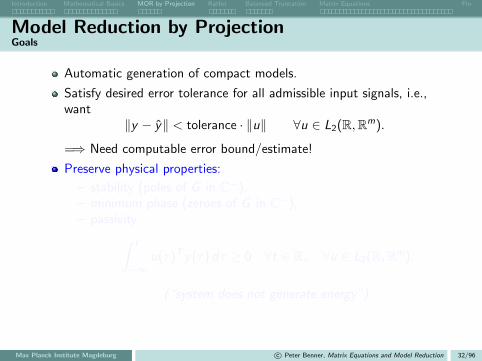
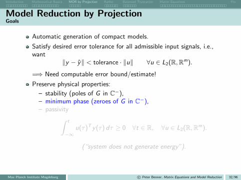
Automatic generation of compact models.
Satisfy desired error tolerance for all admissible input signals, i.e.,want
‖y − y‖ < tolerance · ‖u‖ ∀u ∈ L2(R,Rm).
=⇒ Need computable error bound/estimate!
Preserve physical properties:
– stability (poles of G in C−),– minimum phase (zeroes of G in C−),– passivity∫ t
−∞u(τ)T y(τ) dτ ≥ 0 ∀t ∈ R, ∀u ∈ L2(R,Rm).
(“system does not generate energy”).
Max Planck Institute Magdeburg c© Peter Benner, Matrix Equations and Model Reduction 32/96

Introduction Mathematical Basics MOR by Projection RatInt Balanced Truncation Matrix Equations Fin
Model Reduction by ProjectionGoals
Automatic generation of compact models.
Satisfy desired error tolerance for all admissible input signals, i.e.,want
‖y − y‖ < tolerance · ‖u‖ ∀u ∈ L2(R,Rm).
=⇒ Need computable error bound/estimate!
Preserve physical properties:
– stability (poles of G in C−),– minimum phase (zeroes of G in C−),– passivity∫ t
−∞u(τ)T y(τ) dτ ≥ 0 ∀t ∈ R, ∀u ∈ L2(R,Rm).
(“system does not generate energy”).
Max Planck Institute Magdeburg c© Peter Benner, Matrix Equations and Model Reduction 32/96

Introduction Mathematical Basics MOR by Projection RatInt Balanced Truncation Matrix Equations Fin
Model Reduction by ProjectionProjection Basics
Definition 3.1 (Projector)
A projector is a matrix P ∈ Rn×n with P2 = P. Let V = range (P), then P isprojector onto V. On the other hand, if v1, . . . , vr is a basis of V andV = [ v1, . . . , vr ], then P = V (V TV )−1V T is a projector onto V.
Max Planck Institute Magdeburg c© Peter Benner, Matrix Equations and Model Reduction 33/96

Introduction Mathematical Basics MOR by Projection RatInt Balanced Truncation Matrix Equations Fin
Model Reduction by ProjectionProjection Basics
Definition 3.1 (Projector)
A projector is a matrix P ∈ Rn×n with P2 = P. Let V = range (P), then P isprojector onto V. On the other hand, if v1, . . . , vr is a basis of V andV = [ v1, . . . , vr ], then P = V (V TV )−1V T is a projector onto V.
Lemma 3.2 (Projector Properties)
If P = PT , then P is an orthogonal projector (aka: Galerkin projection),otherwise an oblique projector (aka: Petrov-Galerkin projection).
P is the identity operator on V, i.e., Pv = v ∀v ∈ V.
I − P is the complementary projector onto kerP.
If V is an A-invariant subspace corresponding to a subset of A’s spectrum,then we call P a spectral projector.
Let W ⊂ Rn be another r -dimensional subspace and W = [w1, . . . ,wr ]be a basis matrix for W, then P = V (W TV )−1W T is an obliqueprojector onto V along W.
Max Planck Institute Magdeburg c© Peter Benner, Matrix Equations and Model Reduction 33/96

Introduction Mathematical Basics MOR by Projection RatInt Balanced Truncation Matrix Equations Fin
Model Reduction by ProjectionProjection and Interpolation
Methods:
1 Modal Truncation
2 Rational Interpolation (Pade-Approximation and (rational) KrylovSubspace Methods)
3 Balanced Truncation
4 many more. . .
Joint feature of these methods:computation of reduced-order model (ROM) by projection!
Max Planck Institute Magdeburg c© Peter Benner, Matrix Equations and Model Reduction 34/96

Introduction Mathematical Basics MOR by Projection RatInt Balanced Truncation Matrix Equations Fin
Model Reduction by ProjectionProjection and Interpolation
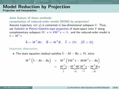
Joint feature of these methods:computation of reduced-order model (ROM) by projection!Assume trajectory x(t; u) is contained in low-dimensional subspace V. Thus,use Galerkin or Petrov-Galerkin-type projection of state-space onto V alongcomplementary subspace W: x ≈ VW T x =: x , where
range (V ) = V, range (W ) =W, W TV = Ir .
Then, with x = W T x , we obtain x ≈ V x so that
‖x − x‖ = ‖x − V x‖,
and the reduced-order model is
A := W TAV , B := W TB, C := CV , (D := D).
Max Planck Institute Magdeburg c© Peter Benner, Matrix Equations and Model Reduction 34/96

Introduction Mathematical Basics MOR by Projection RatInt Balanced Truncation Matrix Equations Fin
Model Reduction by ProjectionProjection and Interpolation
Joint feature of these methods:computation of reduced-order model (ROM) by projection!Assume trajectory x(t; u) is contained in low-dimensional subspace V. Thus,use Galerkin or Petrov-Galerkin-type projection of state-space onto V alongcomplementary subspace W: x ≈ VW T x =: x , and the reduced-order model isx = W T x
A := W TAV , B := W TB, C := CV , (D := D).
Important observation:
The state equation residual satisfies ˙x − Ax − Bu ⊥ W, since
W T(
˙x − Ax − Bu)
= W T(VW T x − AVW T x − Bu
)
Max Planck Institute Magdeburg c© Peter Benner, Matrix Equations and Model Reduction 34/96
Introduction Mathematical Basics MOR by Projection RatInt Balanced Truncation Matrix Equations Fin
Model Reduction by ProjectionProjection and Interpolation
Joint feature of these methods:computation of reduced-order model (ROM) by projection!Assume trajectory x(t; u) is contained in low-dimensional subspace V. Thus,use Galerkin or Petrov-Galerkin-type projection of state-space onto V alongcomplementary subspace W: x ≈ VW T x =: x , and the reduced-order model isx = W T x
A := W TAV , B := W TB, C := CV , (D := D).
Important observation:
The state equation residual satisfies ˙x − Ax − Bu ⊥ W, since
W T(
˙x − Ax − Bu)
= W T(VW T x − AVW T x − Bu
)= W T x︸ ︷︷ ︸
˙x
−W TAV︸ ︷︷ ︸=A
W T x︸ ︷︷ ︸=x
−W TB︸ ︷︷ ︸=B
u
Max Planck Institute Magdeburg c© Peter Benner, Matrix Equations and Model Reduction 34/96

Introduction Mathematical Basics MOR by Projection RatInt Balanced Truncation Matrix Equations Fin
Model Reduction by ProjectionProjection and Interpolation
Joint feature of these methods:computation of reduced-order model (ROM) by projection!Assume trajectory x(t; u) is contained in low-dimensional subspace V. Thus,use Galerkin or Petrov-Galerkin-type projection of state-space onto V alongcomplementary subspace W: x ≈ VW T x =: x , and the reduced-order model isx = W T x
A := W TAV , B := W TB, C := CV , (D := D).
Important observation:
The state equation residual satisfies ˙x − Ax − Bu ⊥ W, since
W T(
˙x − Ax − Bu)
= W T(VW T x − AVW T x − Bu
)= W T x︸ ︷︷ ︸
˙x
−W TAV︸ ︷︷ ︸=A
W T x︸ ︷︷ ︸=x
−W TB︸ ︷︷ ︸=B
u
= ˙x − Ax − Bu = 0.
Max Planck Institute Magdeburg c© Peter Benner, Matrix Equations and Model Reduction 34/96

Introduction Mathematical Basics MOR by Projection RatInt Balanced Truncation Matrix Equations Fin
Model Reduction by ProjectionProjection and Interpolation
Projection Rational InterpolationGiven the ROM
A = W TAV , B = W TB, C = CV , (D = D),
the error transfer function can be written as
G(s)− G(s) =(C(sIn − A)−1B + D
)−(C(sIr − A)−1B + D
)
Max Planck Institute Magdeburg c© Peter Benner, Matrix Equations and Model Reduction 34/96

Introduction Mathematical Basics MOR by Projection RatInt Balanced Truncation Matrix Equations Fin
Model Reduction by ProjectionProjection and Interpolation
Projection Rational InterpolationGiven the ROM
A = W TAV , B = W TB, C = CV , (D = D),
the error transfer function can be written as
G(s)− G(s) =(C(sIn − A)−1B + D
)−(C(sIr − A)−1B + D
)= C
((sIn − A)−1 − V (sIr − A)−1W T
)B
= C(In − V (sIr − A)−1W T (sIn − A)︸ ︷︷ ︸
=:P(s)
)(sIn − A)−1B.
Max Planck Institute Magdeburg c© Peter Benner, Matrix Equations and Model Reduction 34/96

Introduction Mathematical Basics MOR by Projection RatInt Balanced Truncation Matrix Equations Fin
Model Reduction by ProjectionProjection and Interpolation
Projection Rational InterpolationGiven the ROM
A = W TAV , B = W TB, C = CV , (D = D),
the error transfer function can be written as
G(s)− G(s) =(C(sIn − A)−1B + D
)−(C(sIr − A)−1B + D
)= C
(In − V (sIr − A)−1W T (sIn − A)︸ ︷︷ ︸
=:P(s)
)(sIn − A)−1B.
If s∗ ∈ C \ (Λ (A) ∪ Λ (A)), then P(s∗) is a projector onto V:
range (P(s∗)) ⊂ range (V ), all matrices have full rank ⇒ ”=”,
P(s∗)2 = V (s∗Ir − A)−1W T (s∗In − A)V (s∗Ir − A)−1W T (s∗In − A)
= V (s∗Ir − A)−1 (s∗Ir − A)(s∗Ir − A)−1︸ ︷︷ ︸=Ir
W T (s∗In − A) = P(s∗).
Max Planck Institute Magdeburg c© Peter Benner, Matrix Equations and Model Reduction 34/96

Introduction Mathematical Basics MOR by Projection RatInt Balanced Truncation Matrix Equations Fin
Model Reduction by ProjectionProjection and Interpolation
Projection Rational InterpolationGiven the ROM
A = W TAV , B = W TB, C = CV , (D = D),
the error transfer function can be written as
G(s)− G(s) =(C(sIn − A)−1B + D
)−(C(sIr − A)−1B + D
)= C
(In − V (sIr − A)−1W T (sIn − A)︸ ︷︷ ︸
=:P(s)
)(sIn − A)−1B.
If s∗ ∈ C \ (Λ (A) ∪ Λ (A)), then P(s∗) is a projector onto V =⇒
if (s∗In − A)−1B ∈ V, then (In − P(s∗))(s∗In − A)−1B = 0,
hence
G(s∗)− G(s∗) = 0 ⇒ G(s∗) = G(s∗), i.e., G interpolates G in s∗!
Max Planck Institute Magdeburg c© Peter Benner, Matrix Equations and Model Reduction 34/96

Introduction Mathematical Basics MOR by Projection RatInt Balanced Truncation Matrix Equations Fin
Model Reduction by ProjectionProjection and Interpolation
Projection Rational InterpolationGiven the ROM
A = W TAV , B = W TB, C = CV , (D = D),
the error transfer function can be written as
G(s)− G(s) =(C(sIn − A)−1B + D
)−(C(sIr − A)−1B + D
)= C
(In − V (sIr − A)−1W T (sIn − A)︸ ︷︷ ︸
=:P(s)
)(sIn − A)−1B.
Analogously, = C(sIn − A)−1(In − (sIn − A)V (sIr − A)−1W T︸ ︷︷ ︸=:Q(s)
)B.
If s∗ ∈ C \ (Λ (A) ∪ Λ (A)), then Q(s)H is a projector onto W =⇒
if (s∗In − A)−∗CT ∈ W, then C(s∗In − A)−1(In − Q(s∗)) = 0,
hence
G(s∗)− G(s∗) = 0 ⇒ G(s∗) = G(s∗), i.e., G interpolates G in s∗!
Max Planck Institute Magdeburg c© Peter Benner, Matrix Equations and Model Reduction 34/96

Introduction Mathematical Basics MOR by Projection RatInt Balanced Truncation Matrix Equations Fin
Model Reduction by ProjectionProjection and Interpolation
Theorem 3.3 [Grimme ’97, Villemagne/Skelton ’87]
Given the ROM
A = W TAV , B = W TB, C = CV , (D = D),
and s∗ ∈ C \ (Λ (A) ∪ Λ (A)), if either
(s∗In − A)−1B ∈ range (V ), or
(s∗In − A)−∗CT ∈ range (W ),
then the interpolation condition
G (s∗) = G (s∗).
in s∗ holds.
Note: extension to Hermite interpolation conditions later!
Max Planck Institute Magdeburg c© Peter Benner, Matrix Equations and Model Reduction 34/96

Introduction Mathematical Basics MOR by Projection RatInt Balanced Truncation Matrix Equations Fin
Modal Truncation
Basic method:
Assume A is diagonalizable, T−1AT = DA, project state-space onto A-invariantsubspace V = span(t1, . . . , tr ), tk = eigenvectors corresp. to “dominant”modes / eigenvalues of A. Then with
V = T (:, 1 : r) = [ t1, . . . , tr ], W H = T−1(1 : r , :), W = W (V HW )−1,
reduced-order model is
A := W HAV = diag λ1, . . . , λr, B := W HB, C = CV
Also computable by truncation:
T−1AT =
[A
A2
], T−1B =
[BB2
], CT = [ C , C2 ], D = D.
Max Planck Institute Magdeburg c© Peter Benner, Matrix Equations and Model Reduction 35/96
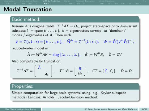
Introduction Mathematical Basics MOR by Projection RatInt Balanced Truncation Matrix Equations Fin
Modal Truncation
Basic method:
Assume A is diagonalizable, T−1AT = DA, project state-space onto A-invariantsubspace V = span(t1, . . . , tr ), tk = eigenvectors corresp. to “dominant”modes / eigenvalues of A. Then with
V = T (:, 1 : r) = [ t1, . . . , tr ], W H = T−1(1 : r , :), W = W (V HW )−1,
reduced-order model is
A := W HAV = diag λ1, . . . , λr, B := W HB, C = CV
Also computable by truncation:
T−1AT =
[A
A2
], T−1B =
[BB2
], CT = [ C , C2 ], D = D.
Properties:Simple computation for large-scale systems, using, e.g., Krylov subspacemethods (Lanczos, Arnoldi), Jacobi-Davidson method.
Max Planck Institute Magdeburg c© Peter Benner, Matrix Equations and Model Reduction 35/96

Introduction Mathematical Basics MOR by Projection RatInt Balanced Truncation Matrix Equations Fin
Modal Truncation
Basic method:
T−1AT =
[A
A2
], T−1B =
[BB2
], CT = [ C , C2 ], D = D.
Properties:Error bound:
‖G − G‖∞ ≤ ‖C2‖‖B2‖1
minλ∈Λ (A2) |Re(λ)| .
Proof:
G(s) = C(sI − A)−1B + D = CTT−1(sI − A)−1TT−1B + D
= CT (sI − T−1AT )−1T−1B + D
= [ C , C2 ]
[(sIr − A)−1
(sIn−r − A2)−1
][BB2
]+ D
= G(s) + C2(sIn−r − A2)−1B2,
Max Planck Institute Magdeburg c© Peter Benner, Matrix Equations and Model Reduction 35/96

Introduction Mathematical Basics MOR by Projection RatInt Balanced Truncation Matrix Equations Fin
Modal Truncation
Basic method:
T−1AT =
[A
A2
], T−1B =
[BB2
], CT = [ C , C2 ], D = D.
Properties:Error bound:
‖G − G‖∞ ≤ ‖C2‖‖B2‖1
minλ∈Λ (A2) |Re(λ)| .
Proof:
G(s) = G(s) + C2(sIn−r − A2)−1B2,
observing that ‖G − G‖∞ = supω∈R σmax(C2(ωIn−r − A2)−1B2), and
C2(ωIn−r − A2)−1B2 = C2diag
(1
ω − λr+1, . . . ,
1
ω − λn
)B2.
Max Planck Institute Magdeburg c© Peter Benner, Matrix Equations and Model Reduction 35/96

Introduction Mathematical Basics MOR by Projection RatInt Balanced Truncation Matrix Equations Fin
Modal Truncation
Basic method:
Assume A is diagonalizable, T−1AT = DA, project state-space onto A-invariantsubspace V = span(t1, . . . , tr ), tk = eigenvectors corresp. to “dominant”modes / eigenvalues of A. Then reduced-order model is
A := W HAV = diag λ1, . . . , λr, B := W HB, C = CV
Also computable by truncation:
T−1AT =
[A
A2
], T−1B =
[BB2
], CT = [ C , C2 ], D = D.
Difficulties:
Eigenvalues contain only limited system information.
Dominance measures are difficult to compute.([Litz ’79] use Jordan canoncial form; otherwise merely heuristic criteria,e.g., [Varga ’95]. Recent improvement: dominant pole algorithm.)
Error bound not computable for really large-scale problems.
Max Planck Institute Magdeburg c© Peter Benner, Matrix Equations and Model Reduction 35/96
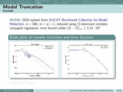
Introduction Mathematical Basics MOR by Projection RatInt Balanced Truncation Matrix Equations Fin
Modal TruncationExample
BEAM, SISO system from SLICOT Benchmark Collection for ModelReduction, n = 348, m = q = 1, reduced using 13 dominant complexconjugate eigenpairs, error bound yields ‖G − G‖∞ ≤ 1.21 · 103
Bode plots of transfer functions and error function
MATLAB R© demo.
Max Planck Institute Magdeburg c© Peter Benner, Matrix Equations and Model Reduction 36/96

Introduction Mathematical Basics MOR by Projection RatInt Balanced Truncation Matrix Equations Fin
Modal TruncationExtensions
Base enrichmentStatic modes are defined by setting x = 0 and assuming unit loads, i.e.,u(t) ≡ ej , j = 1, . . . ,m:
0 = Ax(t) + Bej =⇒ x(t) ≡ −A−1bj .
Projection subspace V is then augmented by A−1[ b1, . . . , bm ] = A−1B.
Interpolation-projection framework =⇒ G (0) = G (0)!
If two sided projection is used, complimentary subspace can beaugmented by A−TCT =⇒ G ′(0) = G ′(0)! (If m 6= q, add randomvectors or delete some of the columns in A−TCT ).
Max Planck Institute Magdeburg c© Peter Benner, Matrix Equations and Model Reduction 37/96
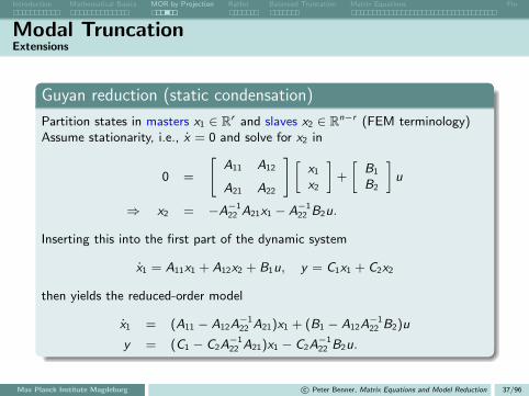
Introduction Mathematical Basics MOR by Projection RatInt Balanced Truncation Matrix Equations Fin
Modal TruncationExtensions
Guyan reduction (static condensation)
Partition states in masters x1 ∈ Rr and slaves x2 ∈ Rn−r (FEM terminology)Assume stationarity, i.e., x = 0 and solve for x2 in
0 =
[A11 A12
A21 A22
][x1
x2
]+
[B1
B2
]u
⇒ x2 = −A−122 A21x1 − A−1
22 B2u.
Inserting this into the first part of the dynamic system
x1 = A11x1 + A12x2 + B1u, y = C1x1 + C2x2
then yields the reduced-order model
x1 = (A11 − A12A−122 A21)x1 + (B1 − A12A
−122 B2)u
y = (C1 − C2A−122 A21)x1 − C2A
−122 B2u.
Max Planck Institute Magdeburg c© Peter Benner, Matrix Equations and Model Reduction 37/96

Introduction Mathematical Basics MOR by Projection RatInt Balanced Truncation Matrix Equations Fin
Modal TruncationDominant Poles
Pole-Residue Form of Transfer FunctionConsider partial fraction expansion of transfer function with D = 0:
G (s) =n∑
k=1
Rk
s − λk
with the residues Rk := (Cxk)(yHk B) ∈ Cq×m.
Max Planck Institute Magdeburg c© Peter Benner, Matrix Equations and Model Reduction 38/96
Introduction Mathematical Basics MOR by Projection RatInt Balanced Truncation Matrix Equations Fin
Modal TruncationDominant Poles
Pole-Residue Form of Transfer FunctionConsider partial fraction expansion of transfer function with D = 0:
G (s) =n∑
k=1
Rk
s − λk
with the residues Rk := (Cxk)(yHk B) ∈ Cq×m.
Note: this follows using the spectral decomposition A = XDX−1, withX = [ x1, . . . , xn] the right and X−1 =: Y = [y1, . . . , yn]H the left eigenvector matrices:
G(s) = C(sI − XDX−1)−1B = CX (sI − diag λ1, . . . , λn)−1YB
= [Cx1, . . . ,Cxn ]
1
s−λ1
. . .1
s−λn
yH
1 B...yHn B
=
n∑k=1
(Cxk )(yHk B)
s − λk.
Max Planck Institute Magdeburg c© Peter Benner, Matrix Equations and Model Reduction 38/96

Introduction Mathematical Basics MOR by Projection RatInt Balanced Truncation Matrix Equations Fin
Modal TruncationDominant Poles
Pole-Residue Form of Transfer FunctionConsider partial fraction expansion of transfer function with D = 0:
G (s) =n∑
k=1
Rk
s − λk
with the residues Rk := (Cxk)(yHk B) ∈ Cq×m.
Note: Rk = (Cxk)(yHk B) are the residues of G in the sense of the residue
theorem of complex analysis:
res (G , λ`) = lims→λ`
(s − λ`)G(s) =n∑
k=1
lims→λ`
s − λ`s − λk︸ ︷︷ ︸
=
0 for k 6= `1 for k = `
Rk = R`.
Max Planck Institute Magdeburg c© Peter Benner, Matrix Equations and Model Reduction 38/96

Introduction Mathematical Basics MOR by Projection RatInt Balanced Truncation Matrix Equations Fin
Modal TruncationDominant Poles
Pole-Residue Form of Transfer FunctionConsider partial fraction expansion of transfer function with D = 0:
G (s) =n∑
k=1
Rk
s − λk
with the residues Rk := (Cxk)(yHk B) ∈ Cq×m.
As projection basis use spaces spanned by right/left eigenvectorscorresponding to dominant poles, i.e.. (λj , xj , yj) with largest
‖Rk‖/| re (λk)|.
RemarkThe dominant modes have most important influence on the input-outputbehavior of the system and are responsible for the ”peaks”’ in the frequencyresponse.
Max Planck Institute Magdeburg c© Peter Benner, Matrix Equations and Model Reduction 38/96

Introduction Mathematical Basics MOR by Projection RatInt Balanced Truncation Matrix Equations Fin
Dominant PolesRandom SISO Example (B, CT ∈ Rn)
0 0.5 1 1.5 2 2.5 3 3.5 4 4.5 50
5
10
ω
‖G(ω
)‖2
exact model, n = 217
Max Planck Institute Magdeburg c© Peter Benner, Matrix Equations and Model Reduction 39/96

Introduction Mathematical Basics MOR by Projection RatInt Balanced Truncation Matrix Equations Fin
Dominant PolesRandom SISO Example (B, CT ∈ Rn)
Max Planck Institute Magdeburg c© Peter Benner, Matrix Equations and Model Reduction 39/96
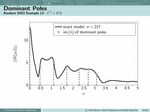
Introduction Mathematical Basics MOR by Projection RatInt Balanced Truncation Matrix Equations Fin
Dominant PolesRandom SISO Example (B, CT ∈ Rn)
0 0.5 1 1.5 2 2.5 3 3.5 4 4.5 50
5
10
ω
‖G(ω
)‖2
exact model, n = 217
im (λ) of dominant poles
Max Planck Institute Magdeburg c© Peter Benner, Matrix Equations and Model Reduction 39/96

Introduction Mathematical Basics MOR by Projection RatInt Balanced Truncation Matrix Equations Fin
Dominant PolesRandom SISO Example (B, CT ∈ Rn)
0 0.5 1 1.5 2 2.5 3 3.5 4 4.5 50
5
10
ω
‖G(ω
)‖2
exact model, n = 217
im (λ) of dominant polesk = 46 dominant poles
k = 46, smallest re (λ) + static modes
Max Planck Institute Magdeburg c© Peter Benner, Matrix Equations and Model Reduction 39/96
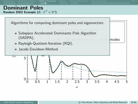
Introduction Mathematical Basics MOR by Projection RatInt Balanced Truncation Matrix Equations Fin
Dominant PolesRandom SISO Example (B, CT ∈ Rn)
0 0.5 1 1.5 2 2.5 3 3.5 4 4.5 50
5
10
ω
‖G(ω
)‖2
exact model, n = 217
im (λ) of dominant polesk = 46 dominant poles
k = 46, smallest re (λ) + static modes
Algorithms for computing dominant poles and eigenvectors:
Subspace Accelerated Dominante Pole Algorithm(SADPA),
Rayleigh-Quotient-Iteration (RQI),
Jacobi-Davidson-Method.
Max Planck Institute Magdeburg c© Peter Benner, Matrix Equations and Model Reduction 39/96

Introduction Mathematical Basics MOR by Projection RatInt Balanced Truncation Matrix Equations Fin
Outline
1 Introduction
2 Mathematical Basics
3 Model Reduction by Projection
4 Interpolatory Model ReductionPade ApproximationA Change of Perspective: Rational InterpolationH2-Optimal Model Reduction
5 Balanced Truncation
6 Solving Large-Scale Matrix Equations
7 Final Remarks
Max Planck Institute Magdeburg c© Peter Benner, Matrix Equations and Model Reduction 40/96

Introduction Mathematical Basics MOR by Projection RatInt Balanced Truncation Matrix Equations Fin
Pade Approximation
Idea:
Consider (even for possibly singular E if λE − A regular):
Ex = Ax + Bu, y = Cx
with transfer function G(s) = C(sE − A)−1B.
Max Planck Institute Magdeburg c© Peter Benner, Matrix Equations and Model Reduction 41/96

Introduction Mathematical Basics MOR by Projection RatInt Balanced Truncation Matrix Equations Fin
Pade Approximation
Idea:
Consider (even for possibly singular E if λE − A regular):
Ex = Ax + Bu, y = Cx
with transfer function G(s) = C(sE − A)−1B.
For s0 6∈ Λ (A,E):
G(s) = C((s0E − A) + (s − s0)E
)−1B
= C(I + (s − s0) (s0E − A)−1E︸ ︷︷ ︸
:=A
)−1
(s0E − A)−1B︸ ︷︷ ︸:=B
= C(I + (s − s0)A
)−1
B
Max Planck Institute Magdeburg c© Peter Benner, Matrix Equations and Model Reduction 41/96
Introduction Mathematical Basics MOR by Projection RatInt Balanced Truncation Matrix Equations Fin
Pade Approximation
Idea:
Consider (even for possibly singular E if λE − A regular):
Ex = Ax + Bu, y = Cx
with transfer function G(s) = C(sE − A)−1B.
For s0 6∈ Λ (A,E):
G(s) = C((s0E − A) + (s − s0)E
)−1B
= C(I + (s − s0) (s0E − A)−1E︸ ︷︷ ︸
:=A
)−1
(s0E − A)−1B︸ ︷︷ ︸:=B
= C(I + (s − s0)A
)−1
B
Neumann Lemma. ‖F‖ < 1 ⇒ I − F invertible, (I − F )−1 =∑∞
k=0 Fk .
Max Planck Institute Magdeburg c© Peter Benner, Matrix Equations and Model Reduction 41/96

Introduction Mathematical Basics MOR by Projection RatInt Balanced Truncation Matrix Equations Fin
Pade Approximation
Idea:
Consider (even for possibly singular E if λE − A regular):
Ex = Ax + Bu, y = Cx
with transfer function G(s) = C(sE − A)−1B.
For s0 6∈ Λ (A,E):
G(s) = C((s0E − A) + (s − s0)E
)−1B
= C(I + (s − s0) (s0E − A)−1E︸ ︷︷ ︸
:=A
)−1
(s0E − A)−1B︸ ︷︷ ︸:=B
= C(I + (s − s0)A
)−1
B = C(I −
(− (s − s0)A
)︸ ︷︷ ︸= F
)−1
B
Neumann Lemma. ‖F‖ < 1 ⇒ I − F invertible, (I − F )−1 =∑∞
k=0 Fk .
Max Planck Institute Magdeburg c© Peter Benner, Matrix Equations and Model Reduction 41/96

Introduction Mathematical Basics MOR by Projection RatInt Balanced Truncation Matrix Equations Fin
Pade Approximation
Idea:
Consider (even for possibly singular E if λE − A regular):
Ex = Ax + Bu, y = Cx
with transfer function G(s) = C(sE − A)−1B.
For s0 6∈ Λ (A,E), and A = (s0E − A)−1E , B = (s0E − A)−1B:
G(s) = C(I + (s − s0)A
)−1
B = C(I −
(− (s − s0)A
)︸ ︷︷ ︸= F
)−1
B
= C
(∞∑k=0
(−1)k(s − s0)k Ak
)B
=∞∑k=0
(−1)kCAk B︸ ︷︷ ︸=: mk
(s − s0)k
= m0 + m1(s − s0) + m2(s − s0)2 + . . .
Max Planck Institute Magdeburg c© Peter Benner, Matrix Equations and Model Reduction 41/96

Introduction Mathematical Basics MOR by Projection RatInt Balanced Truncation Matrix Equations Fin
Pade Approximation
Idea:
Consider (even for possibly singular E if λE − A regular):
Ex = Ax + Bu, y = Cx
with transfer function G(s) = C(sE − A)−1B.
For s0 6∈ Λ (A,E), and A = (s0E − A)−1E , B = (s0E − A)−1B:
G(s) = m0 + m1(s − s0) + m2(s − s0)2 + . . .
with mk = (−1)kCAk B.
– For s0 = 0: mk := −C(A−1E)kA−1B moments.(mk = −CA−(k+1)B for E = In)
– For s0 =∞ and E = In: m0 = 0, mk := CAk−1B for k ≥ 1 Markov parameters.
Max Planck Institute Magdeburg c© Peter Benner, Matrix Equations and Model Reduction 41/96

Introduction Mathematical Basics MOR by Projection RatInt Balanced Truncation Matrix Equations Fin
Pade Approximation
Idea:
Consider (even for possibly singular E if λE − A regular):
Ex = Ax + Bu, y = Cx
with transfer function G(s) = C(sE − A)−1B.
For s0 6∈ Λ (A,E), and A = (s0E − A)−1E , B = (s0E − A)−1B:
G(s) = m0 + m1(s − s0) + m2(s − s0)2 + . . .
with mk = (−1)kCAk B.
As reduced-order model use rth Pade approximant G to G :
G(s) = G(s) +O((s − s0)2r ),
i.e., mk = mk for k = 0, . . . , 2r − 1
moment matching if s0 <∞,
partial realization if s0 =∞.
Max Planck Institute Magdeburg c© Peter Benner, Matrix Equations and Model Reduction 41/96

Introduction Mathematical Basics MOR by Projection RatInt Balanced Truncation Matrix Equations Fin
Pade Approximation
Asymptotic Waveform Evaluation (AWE) [Pillage/Rohrer 1990]
Consider SISO case (m = q = 1) and s0 = 0 for simplicity. With
G(s) =αr−1s
r−1 + αr−2sr−2 + . . .+ α1s + α0
βr s r + βr−1s r−1 + . . .+ β1s + 1,
the solution of the Pade approximation problem is obtained via solving
M
βr...β1
=
−mr
...−m2r−1
,
with the Hankel matrix M =
m0 m1 m2 . . . mr−1
m1 m2 . . .mr
m2 . . .. . . .
.
.
.
.
. . . .. . .
. . .
mr−1 mr . . . m2r−2
.
Then, with β0 := 1: αj =∑j
k=0 mkβj−k .
Max Planck Institute Magdeburg c© Peter Benner, Matrix Equations and Model Reduction 41/96

Introduction Mathematical Basics MOR by Projection RatInt Balanced Truncation Matrix Equations Fin
Pade ApproximationThe Pade-Lanczos Connection [Gallivan/Grimme/Van Dooren 1994, Freund/Feldmann 1994]
Theorem [Grimme ’97, Villemagne/Skelton ’87]
Let s∗ 6∈ Λ (A,E) and
A := (s∗E − A)−1E , B := (s∗E − A)−1B,
A∗ := (s∗E − A)−TET , C := (s∗E − A)−TCT .
If the reduced-order model is obtained by oblique projection onto V ⊂ Rn alongW ⊂ Rn, and
spanB, AB, . . . , AK−1B
⊂ V,
spanC , A∗C , . . . , (A∗)K−1C
⊂ W,
then G(s∗) = G(s∗),dk
dskG(s∗) = dk
dskG(s∗) for k = 1, . . . , `− 1, where
`
= 2K if m = q = 1;≥ bK
mc+ bK
qc if m 6= 1 or q 6= 1.
Max Planck Institute Magdeburg c© Peter Benner, Matrix Equations and Model Reduction 42/96

Introduction Mathematical Basics MOR by Projection RatInt Balanced Truncation Matrix Equations Fin
Pade ApproximationThe Pade-Lanczos Connection [Gallivan/Grimme/Van Dooren 1994, Freund/Feldmann 1994]
Pade-via-Lanczos Method (PVL)
Pade approximation/moment matching yield:
mk =1
k!G (k)(s0) =
1
k!G (k)(s0) = mk , k = 0, . . . , 2K − 1,
i.e., Hermite interpolation in s0.
Recall interpolation via projection result ⇒ moments need not becomputed explicitly; moment matching is equivalent to projectingstate-space onto
V = span(B, AB, . . . , AK−1B) =: KK (A, B)
(where A = (s0E − A)−1E , B = (s0E − A)−1B) along
W = span(C , A∗CT , . . . , (A∗)K−1C) =: KK (A∗, C).
(where A∗ = (s∗E − A)−TET , C = (s∗E − A)−TCT ).
Computation via unsymmetric Lanczos method.
Max Planck Institute Magdeburg c© Peter Benner, Matrix Equations and Model Reduction 43/96

Introduction Mathematical Basics MOR by Projection RatInt Balanced Truncation Matrix Equations Fin
Pade ApproximationThe Pade-Lanczos Connection [Gallivan/Grimme/Van Dooren 1994, Freund/Feldmann 1994]
Pade-via-Lanczos Method (PVL)
Pade approximation/moment matching yield:
mk =1
k!G (k)(s0) =
1
k!G (k)(s0) = mk , k = 0, . . . , 2K − 1,
i.e., Hermite interpolation in s0.
Recall interpolation via projection result ⇒ moments need not becomputed explicitly; moment matching is equivalent to projectingstate-space onto
V = span(B, AB, . . . , AK−1B) =: KK (A, B)
(where A = (s0E − A)−1E , B = (s0E − A)−1B) along
W = span(C , A∗CT , . . . , (A∗)K−1C) =: KK (A∗, C).
(where A∗ = (s∗E − A)−TET , C = (s∗E − A)−TCT ).
Computation via unsymmetric Lanczos method.
Remark: Arnoldi (PRIMA) yields only G(s) = G(s) +O((s − s0)r ).Max Planck Institute Magdeburg c© Peter Benner, Matrix Equations and Model Reduction 43/96

Introduction Mathematical Basics MOR by Projection RatInt Balanced Truncation Matrix Equations Fin
Pade ApproximationThe Pade-Lanczos Connection [Gallivan/Grimme/Van Dooren 1994, Freund/Feldmann 1994]
Pade-via-Lanczos Method (PVL)
Difficulties:
Computable error estimates/bounds for ‖y − y‖2 often very pessimistic orexpensive to evaluate.
Mostly heuristic criteria for choice of expansion points.Optimal choice for second-order systems with proportional/Rayleighdamping (Beattie/Gugercin ’05).
Good approximation quality only locally.
Preservation of physical properties only in special cases (e.g.PRIMA/Arnoldi: V TAV is stable if A is negative definite or dissipative exercises); usually requires post processing which (partially) destroysmoment matching properties.
Max Planck Institute Magdeburg c© Peter Benner, Matrix Equations and Model Reduction 43/96

Introduction Mathematical Basics MOR by Projection RatInt Balanced Truncation Matrix Equations Fin
Interpolatory Model ReductionA Change of Perspective: Rational Interpolation
Computation of reduced-order model by projectionGiven an LTI system x = Ax + Bu, y = Cx with transfer functionG(s) = C(sIn − A)−1B, a reduced-order model is obtained using projectionapproach with V ,W ∈ Rn×r and W TV = Ir by computing
A = W TAV , B = W TB, C = CV .
Petrov-Galerkin-type (two-sided) projection: W 6= V ,
Galerkin-type (one-sided) projection: W = V .
Max Planck Institute Magdeburg c© Peter Benner, Matrix Equations and Model Reduction 44/96
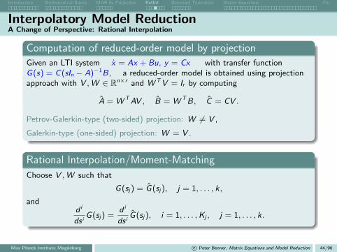
Introduction Mathematical Basics MOR by Projection RatInt Balanced Truncation Matrix Equations Fin
Interpolatory Model ReductionA Change of Perspective: Rational Interpolation
Computation of reduced-order model by projectionGiven an LTI system x = Ax + Bu, y = Cx with transfer functionG(s) = C(sIn − A)−1B, a reduced-order model is obtained using projectionapproach with V ,W ∈ Rn×r and W TV = Ir by computing
A = W TAV , B = W TB, C = CV .
Petrov-Galerkin-type (two-sided) projection: W 6= V ,
Galerkin-type (one-sided) projection: W = V .
Rational Interpolation/Moment-Matching
Choose V ,W such that
G(sj) = G(sj), j = 1, . . . , k,
andd i
ds iG(sj) =
d i
ds iG(sj), i = 1, . . . ,Kj , j = 1, . . . , k.
Max Planck Institute Magdeburg c© Peter Benner, Matrix Equations and Model Reduction 44/96

Introduction Mathematical Basics MOR by Projection RatInt Balanced Truncation Matrix Equations Fin
Interpolatory Model ReductionA Change of Perspective: Rational Interpolation
Theorem (simplified) [Grimme ’97, Villemagne/Skelton ’87]
If
span
(s1In − A)−1B, . . . , (sk In − A)−1B⊂ Ran(V ),
span
(s1In − A)−TCT , . . . , (sk In − A)−TCT⊂ Ran(W ),
then
G (sj) = G (sj),d
dsG (sj) =
d
dsG (sj), for j = 1, . . . , k.
Remarks:
using Galerkin/one-sided projection yields G(sj) = G(sj), but in general
d
dsG(sj) 6=
d
dsG(sj).
Max Planck Institute Magdeburg c© Peter Benner, Matrix Equations and Model Reduction 44/96

Introduction Mathematical Basics MOR by Projection RatInt Balanced Truncation Matrix Equations Fin
Interpolatory Model ReductionA Change of Perspective: Rational Interpolation
Theorem (simplified) [Grimme ’97, Villemagne/Skelton ’87]
If
span
(s1In − A)−1B, . . . , (sk In − A)−1B⊂ Ran(V ),
span
(s1In − A)−TCT , . . . , (sk In − A)−TCT⊂ Ran(W ),
then
G (sj) = G (sj),d
dsG (sj) =
d
dsG (sj), for j = 1, . . . , k.
Remarks:
k = 1, standard Krylov subspace(s) of dimension K moment-matchingmethods/Pade approximation,
d i
ds iG(s1) =
d i
ds iG(s1), i = 0, . . . ,K − 1(+K).
Max Planck Institute Magdeburg c© Peter Benner, Matrix Equations and Model Reduction 44/96

Introduction Mathematical Basics MOR by Projection RatInt Balanced Truncation Matrix Equations Fin
Interpolatory Model ReductionA Change of Perspective: Rational Interpolation
Theorem (simplified) [Grimme ’97, Villemagne/Skelton ’87]
If
span
(s1In − A)−1B, . . . , (sk In − A)−1B⊂ Ran(V ),
span
(s1In − A)−TCT , . . . , (sk In − A)−TCT⊂ Ran(W ),
then
G (sj) = G (sj),d
dsG (sj) =
d
dsG (sj), for j = 1, . . . , k.
Remarks:
computation of V ,W from rational Krylov subspaces, e.g.,
– dual rational Arnoldi/Lanczos [Grimme ’97],
– Iterative Rational Krylov-Algo. [Antoulas/Beattie/Gugercin ’07].
Max Planck Institute Magdeburg c© Peter Benner, Matrix Equations and Model Reduction 44/96

Introduction Mathematical Basics MOR by Projection RatInt Balanced Truncation Matrix Equations Fin
H2-Optimal Model Reduction
Best H2-norm approximation problem
Find arg minG∈H2 of order ≤r‖G − G‖2.
Max Planck Institute Magdeburg c© Peter Benner, Matrix Equations and Model Reduction 45/96

Introduction Mathematical Basics MOR by Projection RatInt Balanced Truncation Matrix Equations Fin
H2-Optimal Model Reduction
Best H2-norm approximation problem
Find arg minG∈H2 of order ≤r‖G − G‖2.
First-order necessary H2-optimality conditions:
For SISO systems
G (−µi ) = G (−µi ),
G ′(−µi ) = G ′(−µi ),
where µi are the poles of the reduced transfer function G .
Max Planck Institute Magdeburg c© Peter Benner, Matrix Equations and Model Reduction 45/96

Introduction Mathematical Basics MOR by Projection RatInt Balanced Truncation Matrix Equations Fin
H2-Optimal Model Reduction
Best H2-norm approximation problem
Find arg minG∈H2 of order ≤r‖G − G‖2.
First-order necessary H2-optimality conditions:
For MIMO systems
G (−µi )Bi = G (−µi )Bi , for i = 1, . . . , r ,
CTi G (−µi ) = CT
i G (−µi ), for i = 1, . . . , r ,
CTi G ′(−µi )Bi = CT
i G ′(−µi )Bi , for i = 1, . . . , r ,
where T−1AT = diag µ1, . . . , µr = spectral decomposition and
B = BTT−T , C = CT .
tangential interpolation conditions.
Max Planck Institute Magdeburg c© Peter Benner, Matrix Equations and Model Reduction 45/96

Introduction Mathematical Basics MOR by Projection RatInt Balanced Truncation Matrix Equations Fin
Interpolatory Model ReductionInterpolation of the Transfer Function by Projection
Construct reduced transfer function by Petrov-Galerkin projectionP = VW T , i.e.
G (s) = CV(sI −W TAV
)−1W TB,
where V and W are given as the rational Krylov subspaces
V =[(−µ1I − A)−1B, . . . , (−µr I − A)−1B
],
W =[(−µ1I − AT )−1CT , . . . , (−µr I − AT )−1CT
].
ThenG (−µi ) = G (−µi ) and G ′(−µi ) = G ′(−µi ),
for i = 1, . . . , r as desired. iterative algorithms (IRKA/MIRIAm) that yield H2-optimal models.
[Gugercin et al. ’06], [Bunse-Gerstner et al. ’07],
[Van Dooren et al. ’08]
Max Planck Institute Magdeburg c© Peter Benner, Matrix Equations and Model Reduction 46/96
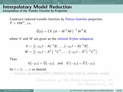
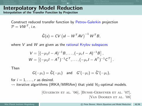
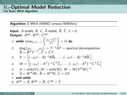
Introduction Mathematical Basics MOR by Projection RatInt Balanced Truncation Matrix Equations Fin
H2-Optimal Model ReductionThe Basic IRKA Algorithm
Algorithm 1 IRKA (MIMO version/MIRIAm)
Input: A stable, B, C , A stable, B, C , δ > 0.Output: Aopt , Bopt , C opt
1: while (maxj=1,...,r
|µj−µold
j ||µj |
> δ) do
2: diag µ1, . . . , µr := T−1AT = spectral decomposition,B = BHT−T , C = CT .
3: V =[(−µ1I − A)−1BB1, . . . , (−µr I − A)−1BBr
]4: W =
[(−µ1I − AT )−1CT C1, . . . , (−µr I − AT )−1CT Cr
]5: V = orth(V ), W = orth(W ), W = W (V HW )−1
6: A = W HAV , B = W HB, C = CV7: end while8: Aopt = A, Bopt = B, C opt = C
Max Planck Institute Magdeburg c© Peter Benner, Matrix Equations and Model Reduction 47/96

Introduction Mathematical Basics MOR by Projection RatInt Balanced Truncation Matrix Equations Fin
Outline
1 Introduction
2 Mathematical Basics
3 Model Reduction by Projection
4 Interpolatory Model Reduction
5 Balanced TruncationThe basic methodTheoretical BackgroundSingular Perturbation ApproximationBalancing-Related Methods
6 Solving Large-Scale Matrix Equations
7 Final Remarks
Max Planck Institute Magdeburg c© Peter Benner, Matrix Equations and Model Reduction 48/96

Introduction Mathematical Basics MOR by Projection RatInt Balanced Truncation Matrix Equations Fin
Balanced Truncation
Basic principle:
Recall: a stable system Σ, realized by (A,B,C ,D), is calledbalanced, if the Gramians, i.e., solutions P,Q of the Lyapunovequations
AP + PAT + BBT = 0, ATQ + QA + CTC = 0,
satisfy: P = Q = diag(σ1, . . . , σn) with σ1 ≥ σ2 ≥ . . . ≥ σn > 0.
Λ (PQ)12 = σ1, . . . , σn are the Hankel singular values (HSVs) of Σ.
Max Planck Institute Magdeburg c© Peter Benner, Matrix Equations and Model Reduction 49/96

Introduction Mathematical Basics MOR by Projection RatInt Balanced Truncation Matrix Equations Fin
Balanced Truncation
Basic principle:
Recall: a stable system Σ, realized by (A,B,C ,D), is calledbalanced, if the Gramians, i.e., solutions P,Q of the Lyapunovequations
AP + PAT + BBT = 0, ATQ + QA + CTC = 0,
satisfy: P = Q = diag(σ1, . . . , σn) with σ1 ≥ σ2 ≥ . . . ≥ σn > 0.
Λ (PQ)12 = σ1, . . . , σn are the Hankel singular values (HSVs) of Σ.
Compute balanced realization of the system via state-spacetransformation
T : (A,B,C ,D) 7→ (TAT−1,TB,CT−1,D)
=
([A11 A12
A21 A22
],
[B1
B2
],[C1 C2
],D
)Truncation (A, B, C , D) := (A11,B1,C1,D).
Max Planck Institute Magdeburg c© Peter Benner, Matrix Equations and Model Reduction 49/96

Introduction Mathematical Basics MOR by Projection RatInt Balanced Truncation Matrix Equations Fin
Balanced Truncation
Motivation:
The HSVs Λ (PQ)12 = σ1, . . . , σn are system invariants: they are
preserved under
T : (A,B,C ,D) 7→ (TAT−1,TB,CT−1,D)
Max Planck Institute Magdeburg c© Peter Benner, Matrix Equations and Model Reduction 49/96
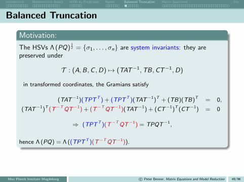
Introduction Mathematical Basics MOR by Projection RatInt Balanced Truncation Matrix Equations Fin
Balanced Truncation
Motivation:
The HSVs Λ (PQ)12 = σ1, . . . , σn are system invariants: they are
preserved under
T : (A,B,C ,D) 7→ (TAT−1,TB,CT−1,D)
in transformed coordinates, the Gramians satisfy
(TAT−1)(TPTT ) + (TPTT )(TAT−1)T + (TB)(TB)T = 0,
(TAT−1)T (T−TQT−1) + (T−TQT−1)(TAT−1) + (CT−1)T (CT−1) = 0
⇒ (TPTT )(T−TQT−1) = TPQT−1,
hence Λ (PQ) = Λ ((TPTT )(T−TQT−1)).
Max Planck Institute Magdeburg c© Peter Benner, Matrix Equations and Model Reduction 49/96

Introduction Mathematical Basics MOR by Projection RatInt Balanced Truncation Matrix Equations Fin
Balanced Truncation
Implementation: SR Method
1 Compute (Cholesky) factors of the Gramians, P = STS , Q = RTR.
2 Compute SVD SRT = [U1, U2 ]
[Σ1
Σ2
][V T
1
V T2
].
3 ROM is (W TAV ,W TB,CV ,D), where
W = RTV1Σ− 1
21 , V = STU1Σ
− 12
1 .
Max Planck Institute Magdeburg c© Peter Benner, Matrix Equations and Model Reduction 49/96
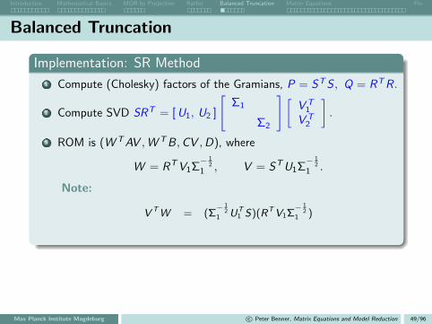
Introduction Mathematical Basics MOR by Projection RatInt Balanced Truncation Matrix Equations Fin
Balanced Truncation
Implementation: SR Method
1 Compute (Cholesky) factors of the Gramians, P = STS , Q = RTR.
2 Compute SVD SRT = [U1, U2 ]
[Σ1
Σ2
][V T
1
V T2
].
3 ROM is (W TAV ,W TB,CV ,D), where
W = RTV1Σ− 1
21 , V = STU1Σ
− 12
1 .
Note:
V TW = (Σ− 1
21 UT
1 S)(RTV1Σ− 1
21 )
Max Planck Institute Magdeburg c© Peter Benner, Matrix Equations and Model Reduction 49/96

Introduction Mathematical Basics MOR by Projection RatInt Balanced Truncation Matrix Equations Fin
Balanced Truncation
Implementation: SR Method
1 Compute (Cholesky) factors of the Gramians, P = STS , Q = RTR.
2 Compute SVD SRT = [U1, U2 ]
[Σ1
Σ2
][V T
1
V T2
].
3 ROM is (W TAV ,W TB,CV ,D), where
W = RTV1Σ− 1
21 , V = STU1Σ
− 12
1 .
Note:
V TW = (Σ− 1
21 UT
1 S)(RTV1Σ− 1
21 ) = Σ
− 12
1 UT1 UΣV TV1Σ
− 12
1
= Σ− 1
21 [ Ir , 0 ]
[Σ1
Σ2
][Ir0
]Σ− 1
21
Max Planck Institute Magdeburg c© Peter Benner, Matrix Equations and Model Reduction 49/96

Introduction Mathematical Basics MOR by Projection RatInt Balanced Truncation Matrix Equations Fin
Balanced Truncation
Implementation: SR Method
1 Compute (Cholesky) factors of the Gramians, P = STS , Q = RTR.
2 Compute SVD SRT = [U1, U2 ]
[Σ1
Σ2
][V T
1
V T2
].
3 ROM is (W TAV ,W TB,CV ,D), where
W = RTV1Σ− 1
21 , V = STU1Σ
− 12
1 .
Note:
V TW = (Σ− 1
21 UT
1 S)(RTV1Σ− 1
21 ) = Σ
− 12
1 UT1 UΣV TV1Σ
− 12
1
= Σ− 1
21 [ Ir , 0 ]
[Σ1
Σ2
] [Ir0
]Σ− 1
21 = Σ
− 12
1 Σ1Σ− 1
21 = Ir
=⇒ VW T is an oblique projector, hence balanced truncation is a
Petrov-Galerkin projection method.
Max Planck Institute Magdeburg c© Peter Benner, Matrix Equations and Model Reduction 49/96

Introduction Mathematical Basics MOR by Projection RatInt Balanced Truncation Matrix Equations Fin
Balanced Truncation
Properties:
Reduced-order model is stable with HSVs σ1, . . . , σr .
Adaptive choice of r via computable error bound:
‖y − y‖2 ≤(
2∑n
k=r+1σk
)‖u‖2.
Max Planck Institute Magdeburg c© Peter Benner, Matrix Equations and Model Reduction 49/96

Introduction Mathematical Basics MOR by Projection RatInt Balanced Truncation Matrix Equations Fin
Balanced TruncationTheoretical Background
Linear, Time-Invariant (LTI) Systems
x = Ax + Bu, A ∈ Rn×n, B ∈ Rn×m,y = Cx + Du, C ∈ Rq×n, D ∈ Rq×m.
Max Planck Institute Magdeburg c© Peter Benner, Matrix Equations and Model Reduction 50/96

Introduction Mathematical Basics MOR by Projection RatInt Balanced Truncation Matrix Equations Fin
Balanced TruncationTheoretical Background
Linear, Time-Invariant (LTI) Systems
x = Ax + Bu, A ∈ Rn×n, B ∈ Rn×m,y = Cx + Du, C ∈ Rq×n, D ∈ Rq×m.
Assumptions (for now): t0 = 0, x0 = x(0) = 0, D = 0.
Max Planck Institute Magdeburg c© Peter Benner, Matrix Equations and Model Reduction 50/96
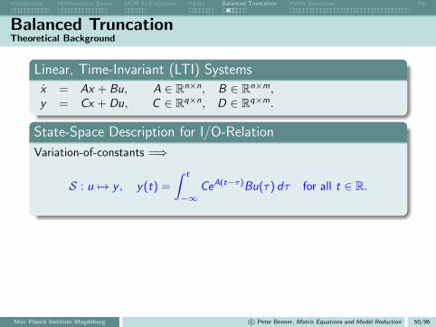
Introduction Mathematical Basics MOR by Projection RatInt Balanced Truncation Matrix Equations Fin
Balanced TruncationTheoretical Background
Linear, Time-Invariant (LTI) Systems
x = Ax + Bu, A ∈ Rn×n, B ∈ Rn×m,y = Cx + Du, C ∈ Rq×n, D ∈ Rq×m.
State-Space Description for I/O-Relation
Variation-of-constants =⇒
S : u 7→ y , y(t) =
∫ t
−∞CeA(t−τ)Bu(τ) dτ for all t ∈ R.
S : U → Y is a linear operator between (function) spaces.
Recall: A ∈ Rn×m is a linear operator, A : Rm → Rn!
Basic Idea: use SVD approximation as for matrix A!
Problem: in general, S does not have a discrete SVD and cantherefore not be approximated as in the matrix case!
Max Planck Institute Magdeburg c© Peter Benner, Matrix Equations and Model Reduction 50/96

Introduction Mathematical Basics MOR by Projection RatInt Balanced Truncation Matrix Equations Fin
Balanced TruncationTheoretical Background
Linear, Time-Invariant (LTI) Systems
x = Ax + Bu, A ∈ Rn×n, B ∈ Rn×m,y = Cx , C ∈ Rq×n.
Alternative to State-Space Operator: Hankel Operator
Instead of
S : u 7→ y , y(t) =
∫ t
−∞CeA(t−τ)Bu(τ) dτ for all t ∈ R.
use Hankel operator
H : u− 7→ y+, y+(t) =
∫ 0
−∞CeA(t−τ)Bu(τ) dτ for all t > 0.
Max Planck Institute Magdeburg c© Peter Benner, Matrix Equations and Model Reduction 51/96

Introduction Mathematical Basics MOR by Projection RatInt Balanced Truncation Matrix Equations Fin
Balanced TruncationTheoretical Background
Linear, Time-Invariant (LTI) Systems
x = Ax + Bu, A ∈ Rn×n, B ∈ Rn×m,y = Cx , C ∈ Rq×n.
Alternative to State-Space Operator: Hankel Operator
Instead of
S : u 7→ y , y(t) =
∫ t
−∞CeA(t−τ)Bu(τ) dτ for all t ∈ R.
use Hankel operator
H : u− 7→ y+, y+(t) =
∫ 0
−∞CeA(t−τ)Bu(τ) dτ for all t > 0.
H compact ⇒ H has discrete SVD
Hankel singular values σj∞j=1 : σ1 ≥ σ2 ≥ . . . ≥ 0.
=⇒ SVD-type approximation of H possible!
Max Planck Institute Magdeburg c© Peter Benner, Matrix Equations and Model Reduction 51/96

Introduction Mathematical Basics MOR by Projection RatInt Balanced Truncation Matrix Equations Fin
Balanced TruncationTheoretical Background
Linear, Time-Invariant (LTI) Systems
x = Ax + Bu, A ∈ Rn×n, B ∈ Rn×m,y = Cx , C ∈ Rq×n.
Alternative to State-Space Operator: Hankel Operator
H compact
⇓H has discrete SVD
⇓Hankel singular values
Max Planck Institute Magdeburg c© Peter Benner, Matrix Equations and Model Reduction 51/96

Introduction Mathematical Basics MOR by Projection RatInt Balanced Truncation Matrix Equations Fin
Balanced TruncationTheoretical Background
Linear, Time-Invariant (LTI) Systems
x = Ax + Bu, A ∈ Rn×n, B ∈ Rn×m,y = Cx , C ∈ Rq×n.
Alternative to State-Space Operator: Hankel Operator
H : u− 7→ y+, y+(t) =
∫ 0
−∞CeA(t−τ)Bu(τ) dτ for all t > 0.
H compact ⇒ H has discrete SVD
⇒ Best approximation problem w.r.t. 2-induced operator norm well-posed
⇒ solution: Adamjan-Arov-Krein (AAK Theory, 1971/78).
But: computationally unfeasible for large-scale systems.
Max Planck Institute Magdeburg c© Peter Benner, Matrix Equations and Model Reduction 51/96

Introduction Mathematical Basics MOR by Projection RatInt Balanced Truncation Matrix Equations Fin
Balanced TruncationThe Hankel Singular Values are Singular Values!
TheoremLet P,Q be the controllability and observability Gramians of an LTIsystem Σ. Then the Hankel singular values Λ (PQ)
12 = σ1, . . . , σn are
the singular values of the Hankel operator associated to Σ.
Max Planck Institute Magdeburg c© Peter Benner, Matrix Equations and Model Reduction 52/96
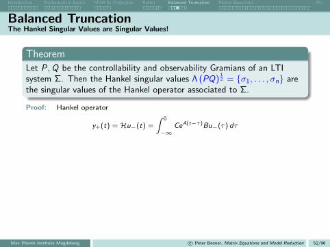
Introduction Mathematical Basics MOR by Projection RatInt Balanced Truncation Matrix Equations Fin
Balanced TruncationThe Hankel Singular Values are Singular Values!
TheoremLet P,Q be the controllability and observability Gramians of an LTIsystem Σ. Then the Hankel singular values Λ (PQ)
12 = σ1, . . . , σn are
the singular values of the Hankel operator associated to Σ.
Proof: Hankel operator
y+(t) = Hu−(t) =
∫ 0
−∞CeA(t−τ)Bu−(τ) dτ
Max Planck Institute Magdeburg c© Peter Benner, Matrix Equations and Model Reduction 52/96

Introduction Mathematical Basics MOR by Projection RatInt Balanced Truncation Matrix Equations Fin
Balanced TruncationThe Hankel Singular Values are Singular Values!
TheoremLet P,Q be the controllability and observability Gramians of an LTIsystem Σ. Then the Hankel singular values Λ (PQ)
12 = σ1, . . . , σn are
the singular values of the Hankel operator associated to Σ.
Proof: Hankel operator
y+(t) = Hu−(t) =
∫ 0
−∞CeA(t−τ)Bu−(τ) dτ =: CeAt
∫ 0
−∞e−AτBu−(τ) dτ︸ ︷︷ ︸
=:z
= CeAtz.
Max Planck Institute Magdeburg c© Peter Benner, Matrix Equations and Model Reduction 52/96
Introduction Mathematical Basics MOR by Projection RatInt Balanced Truncation Matrix Equations Fin
Balanced TruncationThe Hankel Singular Values are Singular Values!
TheoremLet P,Q be the controllability and observability Gramians of an LTIsystem Σ. Then the Hankel singular values Λ (PQ)
12 = σ1, . . . , σn are
the singular values of the Hankel operator associated to Σ.
Proof: Hankel operator
y+(t) = Hu−(t) =
∫ 0
−∞CeA(t−τ)Bu−(τ) dτ = CeAtz.
Singular values of H = square roots of eigenvalues of H∗H,
Max Planck Institute Magdeburg c© Peter Benner, Matrix Equations and Model Reduction 52/96

Introduction Mathematical Basics MOR by Projection RatInt Balanced Truncation Matrix Equations Fin
Balanced TruncationThe Hankel Singular Values are Singular Values!
TheoremLet P,Q be the controllability and observability Gramians of an LTIsystem Σ. Then the Hankel singular values Λ (PQ)
12 = σ1, . . . , σn are
the singular values of the Hankel operator associated to Σ.
Proof: Hankel operator
y+(t) = Hu−(t) =
∫ 0
−∞CeA(t−τ)Bu−(τ) dτ = CeAtz.
Singular values of H = square roots of eigenvalues of H∗H,
H∗y+(t) =
∫ ∞0
BT eAT (τ−t)CT y+(τ) dτ
Max Planck Institute Magdeburg c© Peter Benner, Matrix Equations and Model Reduction 52/96

Introduction Mathematical Basics MOR by Projection RatInt Balanced Truncation Matrix Equations Fin
Balanced TruncationThe Hankel Singular Values are Singular Values!
TheoremLet P,Q be the controllability and observability Gramians of an LTIsystem Σ. Then the Hankel singular values Λ (PQ)
12 = σ1, . . . , σn are
the singular values of the Hankel operator associated to Σ.
Proof: Hankel operator
y+(t) = Hu−(t) =
∫ 0
−∞CeA(t−τ)Bu−(τ) dτ = CeAtz.
Singular values of H = square roots of eigenvalues of H∗H,
H∗y+(t) =
∫ ∞0
BT eAT (τ−t)CT y+(τ) dτ = BT e−AT t
∫ ∞0
eAT τCT y+(τ) dτ.
Max Planck Institute Magdeburg c© Peter Benner, Matrix Equations and Model Reduction 52/96

Introduction Mathematical Basics MOR by Projection RatInt Balanced Truncation Matrix Equations Fin
Balanced TruncationThe Hankel Singular Values are Singular Values!
TheoremLet P,Q be the controllability and observability Gramians of an LTIsystem Σ. Then the Hankel singular values Λ (PQ)
12 = σ1, . . . , σn are
the singular values of the Hankel operator associated to Σ.
Proof: Hankel operator
y+(t) = Hu−(t) =
∫ 0
−∞CeA(t−τ)Bu−(τ) dτ = CeAtz.
Singular values of H = square roots of eigenvalues of H∗H,
H∗y+(t) = = BT e−AT t∫ ∞
0eA
T τCT y+(τ) dτ.
H∗Hu−(t) = BT e−AT t∫ ∞
0eA
T τCTCeAτ z dτ
Max Planck Institute Magdeburg c© Peter Benner, Matrix Equations and Model Reduction 52/96

Introduction Mathematical Basics MOR by Projection RatInt Balanced Truncation Matrix Equations Fin
Balanced TruncationThe Hankel Singular Values are Singular Values!
TheoremLet P,Q be the controllability and observability Gramians of an LTIsystem Σ. Then the Hankel singular values Λ (PQ)
12 = σ1, . . . , σn are
the singular values of the Hankel operator associated to Σ.
Proof: Hankel operator
y+(t) = Hu−(t) =
∫ 0
−∞CeA(t−τ)Bu−(τ) dτ = CeAtz.
Singular values of H = square roots of eigenvalues of H∗H,
H∗y+(t) = = BT e−AT t∫ ∞
0eA
T τCT y+(τ) dτ.
Hence,
H∗Hu−(t) = BT e−AT t∫ ∞
0eA
T τCTCeAτ z dτ
= BT e−AT t∫ ∞
0eA
T τCTCeAτ dτ︸ ︷︷ ︸≡Q
z
Max Planck Institute Magdeburg c© Peter Benner, Matrix Equations and Model Reduction 52/96

Introduction Mathematical Basics MOR by Projection RatInt Balanced Truncation Matrix Equations Fin
Balanced TruncationThe Hankel Singular Values are Singular Values!
TheoremLet P,Q be the controllability and observability Gramians of an LTIsystem Σ. Then the Hankel singular values Λ (PQ)
12 = σ1, . . . , σn are
the singular values of the Hankel operator associated to Σ.
Proof: Hankel operator
y+(t) = Hu−(t) =
∫ 0
−∞CeA(t−τ)Bu−(τ) dτ = CeAtz.
Singular values of H = square roots of eigenvalues of H∗H,
H∗y+(t) = = BT e−AT t∫ ∞
0eA
T τCT y+(τ) dτ.
Hence,
H∗Hu−(t) = BT e−AT t∫ ∞
0eA
T τCTCeAτ z dτ
= BT e−AT tQz
Max Planck Institute Magdeburg c© Peter Benner, Matrix Equations and Model Reduction 52/96

Introduction Mathematical Basics MOR by Projection RatInt Balanced Truncation Matrix Equations Fin
Balanced TruncationThe Hankel Singular Values are Singular Values!
TheoremLet P,Q be the controllability and observability Gramians of an LTIsystem Σ. Then the Hankel singular values Λ (PQ)
12 = σ1, . . . , σn are
the singular values of the Hankel operator associated to Σ.
Proof: Hankel operator
y+(t) = Hu−(t) =
∫ 0
−∞CeA(t−τ)Bu−(τ) dτ = CeAtz.
Singular values of H = square roots of eigenvalues of H∗H,
H∗y+(t) = = BT e−AT t∫ ∞
0eA
T τCT y+(τ) dτ.
Hence,
H∗Hu−(t) = BT e−AT tQz
Max Planck Institute Magdeburg c© Peter Benner, Matrix Equations and Model Reduction 52/96

Introduction Mathematical Basics MOR by Projection RatInt Balanced Truncation Matrix Equations Fin
Balanced TruncationThe Hankel Singular Values are Singular Values!
TheoremLet P,Q be the controllability and observability Gramians of an LTIsystem Σ. Then the Hankel singular values Λ (PQ)
12 = σ1, . . . , σn are
the singular values of the Hankel operator associated to Σ.
Proof: Hankel operator
y+(t) = Hu−(t) =
∫ 0
−∞CeA(t−τ)Bu−(τ) dτ = CeAtz.
Singular values of H = square roots of eigenvalues of H∗H,
H∗y+(t) = = BT e−AT t∫ ∞
0eA
T τCT y+(τ) dτ.
Hence,
H∗Hu−(t) = BT e−AT tQz.
= σ2u−(t).
Max Planck Institute Magdeburg c© Peter Benner, Matrix Equations and Model Reduction 52/96

Introduction Mathematical Basics MOR by Projection RatInt Balanced Truncation Matrix Equations Fin
Balanced TruncationThe Hankel Singular Values are Singular Values!
TheoremLet P,Q be the controllability and observability Gramians of an LTIsystem Σ. Then the Hankel singular values Λ (PQ)
12 = σ1, . . . , σn are
the singular values of the Hankel operator associated to Σ.
Proof: Singular values of H = square roots of eigenvalues of H∗H, Hence,
H∗Hu−(t) = BT e−AT tQz.
= σ2u−(t).
=⇒ u−(t) = 1σ2 B
T e−AT tQz
Max Planck Institute Magdeburg c© Peter Benner, Matrix Equations and Model Reduction 52/96
Introduction Mathematical Basics MOR by Projection RatInt Balanced Truncation Matrix Equations Fin
Balanced TruncationThe Hankel Singular Values are Singular Values!
TheoremLet P,Q be the controllability and observability Gramians of an LTIsystem Σ. Then the Hankel singular values Λ (PQ)
12 = σ1, . . . , σn are
the singular values of the Hankel operator associated to Σ.
Proof: Singular values of H = square roots of eigenvalues of H∗H,
H∗Hu−(t) = BT e−AT tQz.
= σ2u−(t).
=⇒ u−(t) = 1σ2 B
T e−AT tQz =⇒ (recalling z =∫ 0−∞ e−AτBu−(τ) dτ)
Max Planck Institute Magdeburg c© Peter Benner, Matrix Equations and Model Reduction 52/96

Introduction Mathematical Basics MOR by Projection RatInt Balanced Truncation Matrix Equations Fin
Balanced TruncationThe Hankel Singular Values are Singular Values!
TheoremLet P,Q be the controllability and observability Gramians of an LTIsystem Σ. Then the Hankel singular values Λ (PQ)
12 = σ1, . . . , σn are
the singular values of the Hankel operator associated to Σ.
Proof: Singular values of H = square roots of eigenvalues of H∗H,
H∗Hu−(t) = BT e−AT tQz.
= σ2u−(t).
=⇒ u−(t) = 1σ2 B
T e−AT tQz =⇒ (recalling z =∫ 0−∞ e−AτBu−(τ) dτ)
z =
∫ 0
−∞e−AτB
1
σ2BT e−AT τQz dτ
=1
σ2
∫ 0
−∞e−AτBBT e−AT τ dτ Qz
=1
σ2
∫ ∞0
eAtBBT eAT t dt︸ ︷︷ ︸
≡P
Qz
Max Planck Institute Magdeburg c© Peter Benner, Matrix Equations and Model Reduction 52/96

Introduction Mathematical Basics MOR by Projection RatInt Balanced Truncation Matrix Equations Fin
Balanced TruncationThe Hankel Singular Values are Singular Values!
TheoremLet P,Q be the controllability and observability Gramians of an LTIsystem Σ. Then the Hankel singular values Λ (PQ)
12 = σ1, . . . , σn are
the singular values of the Hankel operator associated to Σ.
Proof: Singular values of H = square roots of eigenvalues of H∗H,
H∗Hu−(t) = BT e−AT tQz.
= σ2u−(t).
=⇒ u−(t) = 1σ2 B
T e−AT tQz =⇒ (recalling z =∫ 0−∞ e−AτBu−(τ) dτ)
z =
∫ 0
−∞e−AτB
1
σ2BT e−AT τQz dτ
=1
σ2
∫ ∞0
eAtBBT eAT t dt︸ ︷︷ ︸
≡P
Qz
=1
σ2PQz
Max Planck Institute Magdeburg c© Peter Benner, Matrix Equations and Model Reduction 52/96
Introduction Mathematical Basics MOR by Projection RatInt Balanced Truncation Matrix Equations Fin
Balanced TruncationThe Hankel Singular Values are Singular Values!
TheoremLet P,Q be the controllability and observability Gramians of an LTIsystem Σ. Then the Hankel singular values Λ (PQ)
12 = σ1, . . . , σn are
the singular values of the Hankel operator associated to Σ.
Proof: Singular values of H = square roots of eigenvalues of H∗H,
H∗Hu−(t) = BT e−AT tQz.
= σ2u−(t).
=⇒ u−(t) = 1σ2 B
T e−AT tQz =⇒ (recalling z =∫ 0−∞ e−AτBu−(τ) dτ)
z =
∫ 0
−∞e−AτB
1
σ2BT e−AT τQz dτ
=1
σ2
∫ ∞0
eAtBBT eAT t dt︸ ︷︷ ︸
≡P
Qz
=1
σ2PQz
⇐⇒ PQz = σ2z.
Max Planck Institute Magdeburg c© Peter Benner, Matrix Equations and Model Reduction 52/96

Introduction Mathematical Basics MOR by Projection RatInt Balanced Truncation Matrix Equations Fin
Balanced TruncationThe Hankel Singular Values are Singular Values!
TheoremLet P,Q be the controllability and observability Gramians of an LTIsystem Σ. Then the Hankel singular values Λ (PQ)
12 = σ1, . . . , σn are
the singular values of the Hankel operator associated to Σ.
Theorem
Let the reduced-order system Σ : (A, B, C , D) with r ≤ n be computedby balanced truncation. Then the reduced-order model Σ is balanced,stable, minimal, and its HSVs are σ1, . . . , σr .
Max Planck Institute Magdeburg c© Peter Benner, Matrix Equations and Model Reduction 52/96
Introduction Mathematical Basics MOR by Projection RatInt Balanced Truncation Matrix Equations Fin
Balanced TruncationThe Hankel Singular Values are Singular Values!
Theorem
Let the reduced-order system Σ : (A, B, C , D) with r ≤ n be computedby balanced truncation. Then the reduced-order model Σ is balanced,stable, minimal, and its HSVs are σ1, . . . , σr .
Proof: Note that in balanced coordinates, the Gramians are diagonal and equal to
diag(Σ1,Σ2) = diag(σ1, . . . , σr , σr+1, . . . , σn).
Hence, the Gramian satisfies[A11 A12
A21 A22
] [Σ1
Σ2
]+
[Σ1
Σ2
] [A11 A12
A21 A22
]T+
[B1
B2
] [B1
B2
]T= 0,
whence we obtain the ”controllability Lyapunov equation” of the reduced-order system,
A11Σ1 + Σ1AT11 + B1B
T1 = 0.
The result follows from A = A11, B = B1, Σ1 > 0, the solution theory of Lyapunov
equations and the analogous considerations for the observability Gramian. (Minimality
is a simple consequence of P = Σ1 = Q > 0.)
Max Planck Institute Magdeburg c© Peter Benner, Matrix Equations and Model Reduction 52/96

Introduction Mathematical Basics MOR by Projection RatInt Balanced Truncation Matrix Equations Fin
Singular Perturbation Approximation (aka Balanced Residualization)
Assume the system[x1
x2
]=
[A11 A12
A21 A22
] [x1
x2
]+
[B1
B2
]u, y = [C1, C2 ]
[x1
x2
]+ Du
is in balanced coordinates.
Max Planck Institute Magdeburg c© Peter Benner, Matrix Equations and Model Reduction 53/96

Introduction Mathematical Basics MOR by Projection RatInt Balanced Truncation Matrix Equations Fin
Singular Perturbation Approximation (aka Balanced Residualization)
Assume the system[x1
x2
]=
[A11 A12
A21 A22
] [x1
x2
]+
[B1
B2
]u, y = [C1, C2 ]
[x1
x2
]+ Du
is in balanced coordinates.Balanced truncation would set x2 = 0 and use (A11,B1,C1,D) as reduced-ordermodel, thereby the information present in the remaining model is ignored!
Particularly, if G(0) = G(0) (”zero steady-state error”) is required, one canapply the same condensation technique as in Guyan reduction: instead ofx2 = 0, set x2 = 0. This yields the reduced-order model
x1 = (A11 − A12A−122 A21)x1 + (B1 − A12A
−122 B2)u,
y = (C1 − C2A−122 A21)x1 + (D − C2A
−122 B2)u,
with
the same properties as the reduced-order model w.r.t. stability, minimality,error bound, but D 6= D;
zero steady-state error, G(0) = G(0) as desired.
Max Planck Institute Magdeburg c© Peter Benner, Matrix Equations and Model Reduction 53/96

Introduction Mathematical Basics MOR by Projection RatInt Balanced Truncation Matrix Equations Fin
Singular Perturbation Approximation (aka Balanced Residualization)
Particularly, if G(0) = G(0) (”zero steady-state error”) is required, one canapply the same condensation technique as in Guyan reduction: instead ofx2 = 0, set x2 = 0. This yields the reduced-order model
x1 = (A11 − A12A−122 A21)x1 + (B1 − A12A
−122 B2)u,
y = (C1 − C2A−122 A21)x1 + (D − C2A
−122 B2)u,
with
the same properties as the reduced-order model w.r.t. stability, minimality,error bound, but D 6= D;
zero steady-state error, G(0) = G(0) as desired.
Note:
A22 invertible as in balanced coordinates, A22Σ2 + Σ2AT22 + B2B
T2 = 0 and
(A22,B2) controllable, Σ2 > 0 ⇒ A22 stable.
If the original system is not balanced, first compute a minimal realizationby applying balanced truncation with r = n.
Max Planck Institute Magdeburg c© Peter Benner, Matrix Equations and Model Reduction 53/96

Introduction Mathematical Basics MOR by Projection RatInt Balanced Truncation Matrix Equations Fin
Balancing-Related Methods
Basic Principle
Given positive semidefinite matrices P = STS , Q = RTR, computebalancing state-space transformation so that
P = Q = diag(σ1, . . . , σn) = Σ, σ1 ≥ . . . ≥ σn > 0,
and truncate corresponding realization at size r with σr > σr+1.
Max Planck Institute Magdeburg c© Peter Benner, Matrix Equations and Model Reduction 54/96

Introduction Mathematical Basics MOR by Projection RatInt Balanced Truncation Matrix Equations Fin
Balancing-Related Methods
Basic Principle
Given positive semidefinite matrices P = STS , Q = RTR, computebalancing state-space transformation so that
P = Q = diag(σ1, . . . , σn) = Σ, σ1 ≥ . . . ≥ σn > 0,
and truncate corresponding realization at size r with σr > σr+1.
Classical Balanced Truncation (BT) [Mullis/Roberts ’76, Moore ’81]
P = controllability Gramian of system given by (A,B,C ,D).
Q = observability Gramian of system given by (A,B,C ,D).
P,Q solve dual Lyapunov equations
AP + PAT + BBT = 0, ATQ + QA + CTC = 0.
Max Planck Institute Magdeburg c© Peter Benner, Matrix Equations and Model Reduction 54/96

Introduction Mathematical Basics MOR by Projection RatInt Balanced Truncation Matrix Equations Fin
Balancing-Related Methods
Basic Principle
Given positive semidefinite matrices P = STS , Q = RTR, computebalancing state-space transformation so that
P = Q = diag(σ1, . . . , σn) = Σ, σ1 ≥ . . . ≥ σn > 0,
and truncate corresponding realization at size r with σr > σr+1.
LQG Balanced Truncation (LQGBT) [Jonckheere/Silverman ’83]
P/Q = controllability/observability Gramian of closed-loop systembased on LQG compensator.
P,Q solve dual algebraic Riccati equations (AREs)
0 = AP + PAT − PCTCP + BTB,
0 = ATQ + QA− QBBTQ + CTC .
Max Planck Institute Magdeburg c© Peter Benner, Matrix Equations and Model Reduction 54/96

Introduction Mathematical Basics MOR by Projection RatInt Balanced Truncation Matrix Equations Fin
Balancing-Related Methods
Basic Principle
Given positive semidefinite matrices P = STS , Q = RTR, computebalancing state-space transformation so that
P = Q = diag(σ1, . . . , σn) = Σ, σ1 ≥ . . . ≥ σn > 0,
and truncate corresponding realization at size r with σr > σr+1.
Balanced Stochastic Truncation (BST) [Desai/Pal ’84, Green ’88]
P = controllability Gramian of system given by (A,B,C ,D), i.e.,solution of Lyapunov equation AP + PAT + BBT = 0.
Q = observability Gramian of right spectral factor of powerspectrum of system given by (A,B,C ,D), i.e., solution of ARE
ATQ + QA + QBW (DDT )−1BTWQ + CT (DDT )−1C = 0,
where A := A− BW (DDT )−1C , BW := BDT + PCT .
Max Planck Institute Magdeburg c© Peter Benner, Matrix Equations and Model Reduction 54/96
Introduction Mathematical Basics MOR by Projection RatInt Balanced Truncation Matrix Equations Fin
Balancing-Related Methods
Basic Principle
Given positive semidefinite matrices P = STS , Q = RTR, computebalancing state-space transformation so that
P = Q = diag(σ1, . . . , σn) = Σ, σ1 ≥ . . . ≥ σn > 0,
and truncate corresponding realization at size r with σr > σr+1.
Positive-Real Balanced Truncation (PRBT) [Green ’88]
Based on positive-real equations, related to positive real(Kalman-Yakubovich-Popov-Anderson) lemma.
P,Q solve dual AREs
0 = AP + PAT + PCT R−1CP + BR−1BT ,
0 = ATQ + QA + QBR−1BTQ + CT R−1C ,
where R = D + DT , A = A− BR−1C .
Max Planck Institute Magdeburg c© Peter Benner, Matrix Equations and Model Reduction 54/96

Introduction Mathematical Basics MOR by Projection RatInt Balanced Truncation Matrix Equations Fin
Balancing-Related Methods
Basic Principle
Given positive semidefinite matrices P = STS , Q = RTR, computebalancing state-space transformation so that
P = Q = diag(σ1, . . . , σn) = Σ, σ1 ≥ . . . ≥ σn > 0,
and truncate corresponding realization at size r with σr > σr+1.
Other Balancing-Based Methods
Bounded-real balanced truncation (BRBT) – based on bounded reallemma [Opdenacker/Jonckheere ’88];
H∞ balanced truncation (HinfBT) – closed-loop balancing based onH∞ compensator [Mustafa/Glover ’91].
Both approaches require solution of dual AREs.
Frequency-weighted versions of the above approaches.
Max Planck Institute Magdeburg c© Peter Benner, Matrix Equations and Model Reduction 54/96

Introduction Mathematical Basics MOR by Projection RatInt Balanced Truncation Matrix Equations Fin
Balancing-Related MethodsProperties
Guaranteed preservation of physical properties like– stability (all),– passivity (PRBT),– minimum phase (BST).
Computable error bounds, e.g.,
BT: ‖G − Gr‖∞ ≤ 2n∑
j=r+1
σBTj ,
LQGBT: ‖G − Gr‖∞ ≤ 2n∑
j=r+1
σLQGj√
1+(σLQGj )2
BST: ‖G − Gr‖∞ ≤
n∏j=r+1
1+σBSTj
1−σBSTj
− 1
‖G‖∞,Can be combined with singular perturbation approximation forsteady-state performance.Computations can be modularized.
Max Planck Institute Magdeburg c© Peter Benner, Matrix Equations and Model Reduction 55/96

Introduction Mathematical Basics MOR by Projection RatInt Balanced Truncation Matrix Equations Fin
Outline
1 Introduction
2 Mathematical Basics
3 Model Reduction by Projection
4 Interpolatory Model Reduction
5 Balanced Truncation
6 Solving Large-Scale Matrix EquationsLinear Matrix EquationsNumerical Methods for Solving Lyapunov EquationsSolving Large-Scale Algebraic Riccati EquationsSoftware
7 Final Remarks
Max Planck Institute Magdeburg c© Peter Benner, Matrix Equations and Model Reduction 56/96

Introduction Mathematical Basics MOR by Projection RatInt Balanced Truncation Matrix Equations Fin
Solving Large-Scale Matrix EquationsLarge-Scale Algebraic Lyapunov and Riccati Equations
Algebraic Riccati equation (ARE) for A,G = GT ,W = W T ∈ Rn×n
given and X ∈ Rn×n unknown:
0 = R(X ) := ATX + XA− XGX + W .
G = 0 =⇒ Lyapunov equation:
0 = L(X ) := ATX + XA + W .
Typical situation in model reduction and optimal control problems forsemi-discretized PDEs:
n = 103 – 106 (=⇒ 106 – 1012 unknowns!),
A has sparse representation (A = −M−1S for FEM),
G ,W low-rank with G ,W ∈ BBT ,CTC, whereB ∈ Rn×m, m n, C ∈ Rp×n, p n.
Standard (eigenproblem-based) O(n3) methods are not applicable!
Max Planck Institute Magdeburg c© Peter Benner, Matrix Equations and Model Reduction 57/96

Introduction Mathematical Basics MOR by Projection RatInt Balanced Truncation Matrix Equations Fin
Solving Large-Scale Matrix EquationsLow-Rank Approximation
Consider spectrum of ARE solution (analogous for Lyapunov equations).
Example:
Linear 1D heat equation withpoint control,
Ω = [ 0, 1 ],
FEM discretization using linearB-splines,
h = 1/100 =⇒ n = 101.
Idea: X = XT ≥ 0 =⇒
X = ZZT =n∑
k=1
λkzkzTk ≈ Z (r)(Z (r))T =
r∑k=1
λkzkzTk .
=⇒ Goal: compute Z (r) ∈ Rn×r directly w/o ever forming X !
Max Planck Institute Magdeburg c© Peter Benner, Matrix Equations and Model Reduction 58/96

Introduction Mathematical Basics MOR by Projection RatInt Balanced Truncation Matrix Equations Fin
Solving Large-Scale Matrix EquationsLinear Matrix Equations
Equations without symmetry
Sylvester equation discrete Sylvester equation
AX + XB = W AXB − X = W
with data A ∈ Rn×n, B ∈ Rm×m, W ∈ Rn×m and unknown X ∈ Rn×m.
Equations with symmetry
Lyapunov equation Stein equation (discrete Lyapunov equation)
AX + XAT = W AXAT − X = W
with data A ∈ Rn×n, W = W T ∈ Rn×n and unknown X ∈ Rn×n.
Here: focus on (Sylvester and) Lyapunov equations; analogous resultsand methods for discrete versions exist.
Max Planck Institute Magdeburg c© Peter Benner, Matrix Equations and Model Reduction 59/96

Introduction Mathematical Basics MOR by Projection RatInt Balanced Truncation Matrix Equations Fin
Linear Matrix EquationsSolvability
Using the Kronecker (tensor) product, AX + XB = W is equivalent to((Im ⊗ A) +
(BT ⊗ In
))vec (X ) = vec (W ) .
Hence,
Sylvester equation has a unique solution
⇐⇒
M := (Im ⊗ A) +(BT ⊗ In
)is invertible.
⇐⇒
0 6∈ Λ (M) = Λ ((Im ⊗ A) + (BT ⊗ In)) = λj + µk , | λj ∈ Λ (A), µk ∈ Λ (B).
⇐⇒
Λ (A) ∩ Λ (−B) = ∅
CorollaryA,B Hurwitz =⇒ Sylvester equation has unique solution.
Max Planck Institute Magdeburg c© Peter Benner, Matrix Equations and Model Reduction 60/96

Introduction Mathematical Basics MOR by Projection RatInt Balanced Truncation Matrix Equations Fin
Linear Matrix EquationsComplexity Issues
Solving the Sylvester equation
AX + XB = W
via the equivalent linear system of equations((Im ⊗ A) +
(BT ⊗ In
))vec (X ) = vec (W )
requires
LU factorization of nm × nm matrix; for n ≈ m, complexity is 23n
6;
storing n ·m unknowns: for n ≈ m we have n4 data for X .
Example
n = m = 1, 000 ⇒ Gaussian elimination on an Intel core i7 (Westmere, 6cores, 3.46 GHz 83.2 GFLOP peak) would take > 94 DAYS and 7.3TB of memory!
Max Planck Institute Magdeburg c© Peter Benner, Matrix Equations and Model Reduction 61/96

Introduction Mathematical Basics MOR by Projection RatInt Balanced Truncation Matrix Equations Fin
Numerical Methods for Solving Lyapunov EquationsTraditional Methods
Bartels-Stewart method for Sylvester and Lyapunov equation (lyap);Hessenberg-Schur method for Sylvester equations (lyap);Hammarling’s method for Lyapunov equations AX + XAT + GGT = 0
with A Hurwitz (lyapchol).
All based on the fact that if A,BT are in Schur form, then
M = (Im ⊗ A) +(BT ⊗ In
)is block-upper triangular. Hence, solve Mx = b by back-substitution.
Clever implementation of back-substitution process requires nm(n + m)flops.
For Sylvester eqns., B in Hessenberg form is enough ( Hessenberg-Schur method).
Hammarling’s method computes Cholesky factor Y of X directly.
All methods require Schur decomposition of A and Schur or Hessenbergdecomposition of B ⇒ need QR algorithm which requires 25n3 flops forSchur decomposition.
Not feasible for large-scale problems (n > 10, 000).
Max Planck Institute Magdeburg c© Peter Benner, Matrix Equations and Model Reduction 62/96

Introduction Mathematical Basics MOR by Projection RatInt Balanced Truncation Matrix Equations Fin
Numerical Methods for Solving Lyapunov EquationsThe Sign Function Method
Definition
For Z ∈ Rn×n with Λ (Z ) ∩ ıR = ∅ and Jordan canonical form
Z = S
[J+ 0
0 J−
]S−1
the matrix sign function is
sign (Z ) := S
[Ik 0
0 −In−k
]S−1.
Max Planck Institute Magdeburg c© Peter Benner, Matrix Equations and Model Reduction 63/96

Introduction Mathematical Basics MOR by Projection RatInt Balanced Truncation Matrix Equations Fin
Numerical Methods for Solving Lyapunov EquationsThe Sign Function Method
Definition
For Z ∈ Rn×n with Λ (Z ) ∩ ıR = ∅ and Jordan canonical form
Z = S
[J+ 0
0 J−
]S−1
the matrix sign function is
sign (Z ) := S
[Ik 0
0 −In−k
]S−1.
Lemma
Let T ∈ Rn×n be nonsingular and Z as before, then
sign(TZT−1
)= T sign (Z )T−1
Max Planck Institute Magdeburg c© Peter Benner, Matrix Equations and Model Reduction 63/96
Introduction Mathematical Basics MOR by Projection RatInt Balanced Truncation Matrix Equations Fin
Numerical Methods for Solving Lyapunov EquationsThe Sign Function Method
Computation of sign (Z )
sign (Z ) is root of In =⇒ use Newton’s method to compute it:
Z0 ← Z , Zj+1 ←1
2
(cjZj +
1
cjZ−1j
), j = 1, 2, . . .
=⇒ sign (Z ) = limj→∞ Zj .
cj > 0 is scaling parameter for convergence acceleration and rounding errorminimization, e.g.
cj =
√‖Z−1
j ‖F‖Zj‖F
,
based on “equilibrating” the norms of the two summands [Higham ’86].
Max Planck Institute Magdeburg c© Peter Benner, Matrix Equations and Model Reduction 63/96

Introduction Mathematical Basics MOR by Projection RatInt Balanced Truncation Matrix Equations Fin
Solving Lyapunov Equations with the Matrix Sign Function Method
Key observation:If X ∈ Rn×n is a solution of AX + XAT + W = 0, then[
In −X
0 In
]︸ ︷︷ ︸
=T−1
[A W
0 −AT
]︸ ︷︷ ︸
=:H
[In X
0 In
]︸ ︷︷ ︸
=:T
=
[A 0
0 −AT
].
Hence, if A is Hurwitz (i.e., asymptotically stable), then
sign (H) = sign
(T
[A 0
0 −AT
]T−1
)= T sign
([A 0
0 −AT
])T−1
=
[−In 2X
0 In
].
Max Planck Institute Magdeburg c© Peter Benner, Matrix Equations and Model Reduction 64/96

Introduction Mathematical Basics MOR by Projection RatInt Balanced Truncation Matrix Equations Fin
Solving Lyapunov Equations with the Matrix Sign Function Method
Apply sign function iteration Z ← 12 (Z + Z−1) to H =
[A W
0 −AT
]:
H + H−1 =
[A W0 −AT
]+
[A−1 A−1WA−T
0 −A−T]
=⇒ Sign function iteration for Lyapunov equation:
A0 ←A, Aj+1 ← 12
(Aj + A−1
j
),
W0←G , Wj+1← 12
(Wj + A−1
j WjA−Tj
),
j = 0, 1, 2, . . . .
Define A∞ := limj→∞ Aj , W∞ := limj→∞Wj .
TheoremIf A is Hurwitz, then
A∞ = −In and X =1
2W∞.
Max Planck Institute Magdeburg c© Peter Benner, Matrix Equations and Model Reduction 65/96

Introduction Mathematical Basics MOR by Projection RatInt Balanced Truncation Matrix Equations Fin
Solving Lyapunov Equations with the Matrix Sign Function MethodFactored form
Recall sign function iteration for AX + XAT + W = 0:
A0 ←A, Aj+1 ← 12
(Aj + A−1
j
),
W0←G , Wj+1← 12
(Wj + A−1
j WjA−Tj
),
j = 0, 1, 2, . . . .
Now consider the second iteration for W = BBT , starting withW0 = BBT =: B0B
T0 :
1
2
(Wj + A−1
j WjA−Tj
)=
1
2
(BjB
Tj + A−1
j BjBTj A−T
j
)=
1
2
[Bj A−1
j Bj
] [Bj A−1
j Bj
]T.
Hence, obtain factored iteration
Bj+1 ←1√2
[Bj A−1
j Bj
]with S := 1√
2limj→∞ Bj and X = SST .
Max Planck Institute Magdeburg c© Peter Benner, Matrix Equations and Model Reduction 66/96
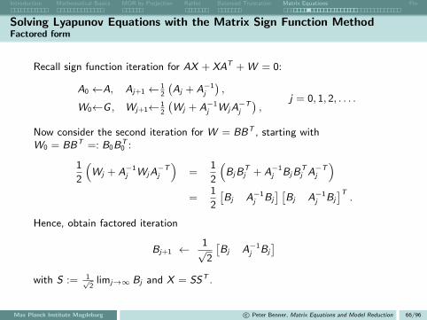

Introduction Mathematical Basics MOR by Projection RatInt Balanced Truncation Matrix Equations Fin
Solving Lyapunov Equations with the Matrix Sign Function MethodFactored form [B./Quintana-Ortı ’97]
Factored sign function iteration for A(SST ) + (SST )AT + BBT = 0
A0←A, Aj+1← 12
(Aj + A−1
j
),
B0←B, Bj+1← 1√2
[Bj A−1
j Bj
],
j = 0, 1, 2, . . . .
Remarks:
To get both Gramians, run in parallel
Cj+1 ←1√2
[Cj
CjA−1j
].
To avoid growth in numbers of columns of Bj (or rows of Cj): columncompression by RRLQ or truncated SVD.
Several options to incorporate scaling, e.g., scale ”A”-iteration only.
Simple stopping cirterion: ‖Aj + In‖F ≤ tol .
Max Planck Institute Magdeburg c© Peter Benner, Matrix Equations and Model Reduction 67/96

Introduction Mathematical Basics MOR by Projection RatInt Balanced Truncation Matrix Equations Fin
Numerical Methods for Solving Lyapunov EquationsThe ADI Method
Recall Peaceman Rachford ADI:Consider Au = s where A ∈ Rn×n spd, s ∈ Rn. ADI Iteration Idea:Decompose A = H + V with H,V ∈ Rn×n such that
(H + pI )v = r(V + pI )w = t
can be solved easily/efficiently.
ADI IterationIf H,V spd ⇒ ∃pk , k = 1, 2, . . . such that
u0 = 0(H + pk I )uk− 1
2= (pk I − V )uk−1 + s
(V + pk I )uk = (pk I − H)uk− 12
+ s
converges to u ∈ Rn solving Au = s.
Max Planck Institute Magdeburg c© Peter Benner, Matrix Equations and Model Reduction 68/96

Introduction Mathematical Basics MOR by Projection RatInt Balanced Truncation Matrix Equations Fin
Numerical Methods for Solving Lyapunov Equations
The Lyapunov operator
L : P 7→ AX + XAT
can be decomposed into the linear operators
LH : X 7→ AX , LV : X 7→ XAT .
In analogy to the standard ADI method we find the
ADI iteration for the Lyapunov equation [Wachspress ’88]
X0 = 0(A + pk I )Xk− 1
2= −W − Xk−1(AT − pk I )
(A + pk I )XTk = −W − XT
k− 12
(AT − pk I ).
Max Planck Institute Magdeburg c© Peter Benner, Matrix Equations and Model Reduction 69/96

Introduction Mathematical Basics MOR by Projection RatInt Balanced Truncation Matrix Equations Fin
Numerical Methods for Solving Lyapunov EquationsLow-Rank ADI
Consider AX + XAT = −BBT for stable A; B ∈ Rn×m with m n.
ADI iteration for the Lyapunov equation [Wachspress ’95]
For k = 1, . . . , kmax
X0 = 0(A + pk I )Xk− 1
2= −BBT − Xk−1(AT − pk I )
(A + pk I )XTk = −BBT − XT
k− 12
(AT − pk I )
Rewrite as one step iteration and factorize Xk = ZkZTk , k = 0, . . . , kmax
Z0ZT0 = 0
ZkZTk = −2pk(A + pk I )
−1BBT (A + pk I )−T
+(A + pk I )−1(A− pk I )Zk−1Z
Tk−1(A− pk I )
T (A + pk I )−T
. . . low-rank Cholesky factor ADI[Penzl ’97/’00, Li/White ’99/’02, B./Li/Penzl ‘99/’08, Gugercin/Sorensen/Antoulas ’03]
Max Planck Institute Magdeburg c© Peter Benner, Matrix Equations and Model Reduction 70/96

Introduction Mathematical Basics MOR by Projection RatInt Balanced Truncation Matrix Equations Fin
Solving Large-Scale Matrix EquationsNumerical Methods for Solving Lyapunov Equations
Zk = [√−2pk(A + pk I )
−1B, (A + pk I )−1(A− pk I )Zk−1]
[Penzl ’00]
Observing that (A− pi I ), (A + pk I )−1 commute, we rewrite Zkmax as
Zkmax = [zkmax , Pkmax−1zkmax , Pkmax−2(Pkmax−1zkmax ), . . . , P1(P2 · · ·Pkmax−1zkmax )],
[Li/White ’02]
wherezkmax =
√−2pkmax (A + pkmax I )
−1B
and
Pi :=
√−2pi√−2pi+1
[I − (pi + pi+1)(A + pi I )
−1].
Max Planck Institute Magdeburg c© Peter Benner, Matrix Equations and Model Reduction 71/96

Introduction Mathematical Basics MOR by Projection RatInt Balanced Truncation Matrix Equations Fin
Numerical Methods for Solving Lyapunov EquationsLyapunov equation 0 = AX + XAT + BBT .
Algorithm [Penzl ’97/’00, Li/White ’99/’02, B. 04, B./Li/Penzl ’99/’08]
V1 ←√−2 re p1(A + p1I )
−1B, Z1 ← V1
FOR k = 2, 3, . . .
Vk ←√
re pkre pk−1
(Vk−1 − (pk + pk−1)(A + pk I )
−1Vk−1
)Zk ←
[Zk−1 Vk
]Zk ← rrlq(Zk , τ) column compression
At convergence, ZkmaxZTkmax≈ X , where (without column compression)
Zkmax =[V1 . . . Vkmax
], Vk = ∈ Cn×m.
Note: Implementation in real arithmetic possible by combining two steps
[B./Li/Penzl ’99/’08] or using new idea employing the relation of 2 consecutive
complex factors [B./Kurschner/Saak ’11].
Max Planck Institute Magdeburg c© Peter Benner, Matrix Equations and Model Reduction 72/96
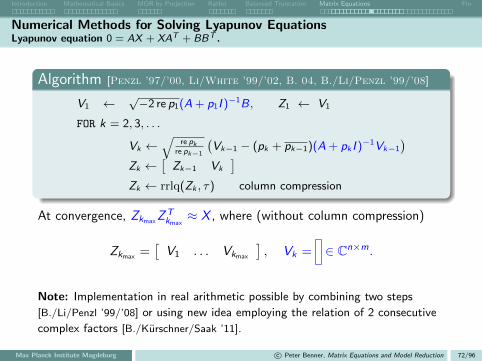

Introduction Mathematical Basics MOR by Projection RatInt Balanced Truncation Matrix Equations Fin
Numerical Results for ADIOptimal Cooling of Steel Profiles
Mathematical model: boundary control forlinearized 2D heat equation.
c · ρ ∂∂t
x = λ∆x , ξ ∈ Ω
λ∂
∂nx = κ(uk − x), ξ ∈ Γk , 1 ≤ k ≤ 7,
∂
∂nx = 0, ξ ∈ Γ7.
=⇒ m = 7, q = 6.
FEM Discretization, different models forinitial mesh (n = 371),1, 2, 3, 4 steps of mesh refinement ⇒n = 1357, 5177, 20209, 79841. 2
34
9 10
1516
22
34
43
47
51
55
60 63
8392
Source: Physical model: courtesy of Mannesmann/Demag.
Math. model: Troltzsch/Unger 1999/2001, Penzl 1999, Saak 2003.
Max Planck Institute Magdeburg c© Peter Benner, Matrix Equations and Model Reduction 73/96

Introduction Mathematical Basics MOR by Projection RatInt Balanced Truncation Matrix Equations Fin
Numerical Results for ADIOptimal Cooling of Steel Profiles
Solve dual Lyapunov equations needed for balanced truncation, i.e.,
APMT + MPAT + BBT = 0, ATQM + MTQA + CTC = 0,
for n = 79, 841.25 shifts chosen by Penzl heuristic from 50/25 Ritz values of A oflargest/smallest magnitude, no column compression performed.No factorization of mass matrix required.Computations done on Core2Duo at 2.8GHz with 3GB RAM and32Bit-MATLAB.
CPU times: 626 / 356 sec.Max Planck Institute Magdeburg c© Peter Benner, Matrix Equations and Model Reduction 74/96

Introduction Mathematical Basics MOR by Projection RatInt Balanced Truncation Matrix Equations Fin
Numerical Results for ADIScaling / Mesh Independence Computations by Martin Kohler ’10
A ∈ Rn×n ≡ FDM matrix for 2D heat equation on [0, 1]2 (Lyapackbenchmark demo l1, m = 1).
16 shifts chosen by Penzl heuristic from 50/25 Ritz values of A oflargest/smallest magnitude.
Computations on 2 dual core Intel Xeon 5160 with 16 GB RAM usingM.E.S.S. (http://svncsc.mpi-magdeburg.mpg.de/trac/messtrac/).
Max Planck Institute Magdeburg c© Peter Benner, Matrix Equations and Model Reduction 75/96

Introduction Mathematical Basics MOR by Projection RatInt Balanced Truncation Matrix Equations Fin
Numerical Results for ADIScaling / Mesh Independence Computations by Martin Kohler ’10
A ∈ Rn×n ≡ FDM matrix for 2D heat equation on [0, 1]2 (Lyapackbenchmark demo l1, m = 1).
16 shifts chosen by Penzl heuristic from 50/25 Ritz values of A oflargest/smallest magnitude.
Computations on 2 dual core Intel Xeon 5160 with 16 GB RAM usingM.E.S.S. (http://svncsc.mpi-magdeburg.mpg.de/trac/messtrac/).
CPU Timesn M.E.S.S.1 (C) LyaPack M.E.S.S. (MATLAB)
100 0.023 0.124 0.158625 0.042 0.104 0.227
2,500 0.159 0.702 0.98910,000 0.965 6.22 5.64440,000 11.09 71.48 34.5590,000 34.67 418.5 90.49
160,000 109.3 out of memory 219.9250,000 193.7 out of memory 403.8562,500 930.1 out of memory 1216.7
1,000,000 2220.0 out of memory 2428.6
Max Planck Institute Magdeburg c© Peter Benner, Matrix Equations and Model Reduction 75/96

Introduction Mathematical Basics MOR by Projection RatInt Balanced Truncation Matrix Equations Fin
Numerical Results for ADIScaling / Mesh Independence Computations by Martin Kohler ’10
A ∈ Rn×n ≡ FDM matrix for 2D heat equation on [0, 1]2 (Lyapackbenchmark demo l1, m = 1).
16 shifts chosen by Penzl heuristic from 50/25 Ritz values of A oflargest/smallest magnitude.
Computations on 2 dual core Intel Xeon 5160 with 16 GB RAM usingM.E.S.S. (http://svncsc.mpi-magdeburg.mpg.de/trac/messtrac/).
Note: for n = 1, 000, 000, first sparse LU needs ∼ 1, 100 sec., usingUMFPACK this reduces to 30 sec.
Max Planck Institute Magdeburg c© Peter Benner, Matrix Equations and Model Reduction 75/96

Introduction Mathematical Basics MOR by Projection RatInt Balanced Truncation Matrix Equations Fin
Factored Galerkin-ADI IterationLyapunov equation 0 = AX + XAT + BBT
Projection-based methods for Lyapunov equations with A + AT < 0:1 Compute orthonormal basis range (Z), Z ∈ Rn×r , for subspace Z ⊂ Rn,
dimZ = r .2 Set A := ZTAZ , B := ZTB.3 Solve small-size Lyapunov equation AX + X AT + BBT = 0.4 Use X ≈ ZXZT .
Examples:
Krylov subspace methods, i.e., for m = 1:
Z = K(A,B, r) = spanB,AB,A2B, . . . ,Ar−1B
[Saad ’90, Jaimoukha/Kasenally ’94, Jbilou ’02–’08].
K-PIK [Simoncini ’07],
Z = K(A,B, r) ∪ K(A−1,B, r).
Rational Krylov [Druskin/Simoncini ’11] ( exercises).
Max Planck Institute Magdeburg c© Peter Benner, Matrix Equations and Model Reduction 76/96

Introduction Mathematical Basics MOR by Projection RatInt Balanced Truncation Matrix Equations Fin
Factored Galerkin-ADI IterationLyapunov equation 0 = AX + XAT + BBT
Projection-based methods for Lyapunov equations with A + AT < 0:1 Compute orthonormal basis range (Z), Z ∈ Rn×r , for subspace Z ⊂ Rn,
dimZ = r .2 Set A := ZTAZ , B := ZTB.3 Solve small-size Lyapunov equation AX + X AT + BBT = 0.4 Use X ≈ ZXZT .
Examples:
ADI subspace [B./R.-C. Li/Truhar ’08]:
Z = colspan[V1, . . . , Vr
].
Note:1 ADI subspace is rational Krylov subspace [J.-R. Li/White ’02].2 Similar approach: ADI-preconditioned global Arnoldi method
[Jbilou ’08].
Max Planck Institute Magdeburg c© Peter Benner, Matrix Equations and Model Reduction 76/96

Introduction Mathematical Basics MOR by Projection RatInt Balanced Truncation Matrix Equations Fin
Numerical Methods for Solving Lyapunov EquationsNumerical examples for Galerkin-ADI
FEM semi-discretized control problem for parabolic PDE:
optimal cooling of rail profiles,
n = 20, 209, m = 7, q = 6.
Good ADI shifts
CPU times: 80s (projection every 5th ADI step) vs. 94s (no projection).
Computations by Jens Saak ’10.Max Planck Institute Magdeburg c© Peter Benner, Matrix Equations and Model Reduction 77/96

Introduction Mathematical Basics MOR by Projection RatInt Balanced Truncation Matrix Equations Fin
Numerical Methods for Solving Lyapunov EquationsNumerical examples for Galerkin-ADI
FEM semi-discretized control problem for parabolic PDE:
optimal cooling of rail profiles,
n = 20, 209, m = 7, q = 6.
Bad ADI shifts
CPU times: 368s (projection every 5th ADI step) vs. 1207s (no projection).
Computations by Jens Saak ’10.Max Planck Institute Magdeburg c© Peter Benner, Matrix Equations and Model Reduction 77/96

Introduction Mathematical Basics MOR by Projection RatInt Balanced Truncation Matrix Equations Fin
Numerical Methods for Solving Lyapunov EquationsNumerical examples for Galerkin-ADI: optimal cooling of rail profiles, n = 79, 841.
M.E.S.S. w/o Galerkin projection and column compression
Rank of solution factors: 532 / 426
M.E.S.S. with Galerkin projection and column compression
Rank of solution factors: 269 / 205
Max Planck Institute Magdeburg c© Peter Benner, Matrix Equations and Model Reduction 78/96
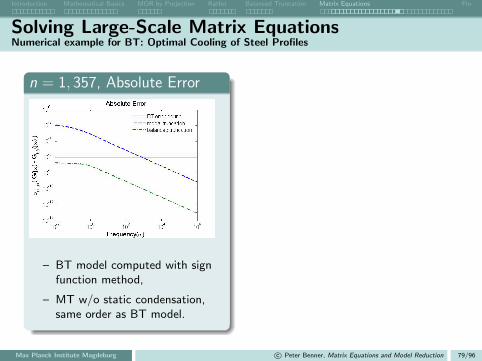
Introduction Mathematical Basics MOR by Projection RatInt Balanced Truncation Matrix Equations Fin
Solving Large-Scale Matrix EquationsNumerical example for BT: Optimal Cooling of Steel Profiles
n = 1, 357, Absolute Error
– BT model computed with signfunction method,
– MT w/o static condensation,same order as BT model.
n = 79, 841, Absolute Error
– BT model computed usingM.E.S.S. in MATLAB,
– dualcore, computation time:<10 min.
Max Planck Institute Magdeburg c© Peter Benner, Matrix Equations and Model Reduction 79/96

Introduction Mathematical Basics MOR by Projection RatInt Balanced Truncation Matrix Equations Fin
Solving Large-Scale Matrix EquationsNumerical example for BT: Microgyroscope (Butterfly Gyro)
FEM discretization of structure dynamical model using quadratictetrahedral elements (ANSYS-SOLID187) n = 34, 722, m = 1, q = 12.
Reduced model computed using SpaRed, r = 30.
Frequency Repsonse Analysis Hankel Singular Values
Max Planck Institute Magdeburg c© Peter Benner, Matrix Equations and Model Reduction 80/96

Introduction Mathematical Basics MOR by Projection RatInt Balanced Truncation Matrix Equations Fin
Solving Large-Scale Matrix EquationsNumerical example for BT: Microgyroscope (Butterfly Gyro)
FEM discretization of structure dynamical model using quadratictetrahedral elements (ANSYS-SOLID187) n = 34, 722, m = 1, q = 12.
Reduced model computed using SpaRed, r = 30.
Frequency Repsonse Analysis
Hankel Singular Values
Max Planck Institute Magdeburg c© Peter Benner, Matrix Equations and Model Reduction 80/96

Introduction Mathematical Basics MOR by Projection RatInt Balanced Truncation Matrix Equations Fin
Solving Large-Scale Matrix EquationsNumerical example for BT: Microgyroscope (Butterfly Gyro)
FEM discretization of structure dynamical model using quadratictetrahedral elements (ANSYS-SOLID187) n = 34, 722, m = 1, q = 12.
Reduced model computed using SpaRed, r = 30.
Frequency Repsonse Analysis Hankel Singular Values
Max Planck Institute Magdeburg c© Peter Benner, Matrix Equations and Model Reduction 80/96

Introduction Mathematical Basics MOR by Projection RatInt Balanced Truncation Matrix Equations Fin
Solving Large-Scale Algebraic Riccati EquationsTheory [Lancaster/Rodman ’95]
TheoremConsider the (continuous-time) algebraic Riccati equation (ARE)
0 = R(X ) = CTC + ATX + XA− XBBTX ,
with A ∈ Rn×n, B ∈ Rn×m, C ∈ Rq×n, (A,B) stabilizable, (A,C) detectable.Then:
(a) There exists a unique stabilizing X∗ ∈ X ∈ Rn×n |R(X ) = 0 , i.e.,Λ (A− BBTX∗) ∈ C−.
(b) X∗ = XT∗ ≥ 0 and X∗ ≥ X for all X ∈ X ∈ Rn×n |R(X ) = 0 .
(c) If (A,C) observable, then X∗ > 0.
(d) span
[In−X∗
]is the unique invariant subspace of the Hamiltonian
matrix
H =
[A BBT
CTC −AT
]corresponding to Λ (H) ∩ C−.
Max Planck Institute Magdeburg c© Peter Benner, Matrix Equations and Model Reduction 81/96

Introduction Mathematical Basics MOR by Projection RatInt Balanced Truncation Matrix Equations Fin
Solving Large-Scale Algebraic Riccati EquationsNumerical Methods [Bini/Iannazzo/Meini ’12]
Numerical Methods (incomplete list)
Invariant subspace methods ( eigenproblem for Hamiltonian matrix):
– Schur vector method (care) [Laub ’79]
– Hamiltonian SR algorithm [Bunse-Gerstner/Mehrmann ’86]
– Symplectic URV-based method[B./Mehrmann/Xu ’97/’98, Chu/Liu/Mehrmann ’07]
Spectral projection methods
– Sign function method [Roberts ’71, Byers ’87]
– Disk function method [Bai/Demmel/Gu ’94, B. ’97]
(rational, global) Krylov subspace techniques[Jaimoukha/Kasenally ’94, Jbilou ’03/’06, Heyouni/Jbilou ’09]
Newton’s method
– Kleinman iteration [Kleinman ’68]
– Line search acceleration [B./Byers ’98]
– Newton-ADI [B./J.-R. Li/Penzl ’99/’08]
– Inexact Newton [Feitzinger/Hylla/Sachs ’09]
Max Planck Institute Magdeburg c© Peter Benner, Matrix Equations and Model Reduction 82/96

Introduction Mathematical Basics MOR by Projection RatInt Balanced Truncation Matrix Equations Fin
Solving Large-Scale Algebraic Riccati EquationsNewton’s Method for AREs[Kleinman ’68, Mehrmann ’91, Lancaster/Rodman ’95, B./Byers ’94/’98, B. ’97, Guo/Laub ’99]
Consider 0 = R(X ) = CTC + ATX + XA− XBBTX .
Frechet derivative of R(X ) at X :
R′X : Z → (A− BBTX )TZ + Z (A− BBTX ).
Newton-Kantorovich method:
Xj+1 = Xj −(R′Xj
)−1
R(Xj), j = 0, 1, 2, . . .
Newton’s method (with line search) for AREs
FOR j = 0, 1, . . .
1 Aj ← A− BBTXj =: A− BKj .
2 Solve the Lyapunov equation ATj Nj + NjAj = −R(Xj).
3 Xj+1 ← Xj + tjNj .
END FOR j
Max Planck Institute Magdeburg c© Peter Benner, Matrix Equations and Model Reduction 83/96

Introduction Mathematical Basics MOR by Projection RatInt Balanced Truncation Matrix Equations Fin
Newton’s Method for AREsProperties and Implementation
Convergence for K0 stabilizing:
Aj = A− BKj = A− BBTXj is stable ∀ j ≥ 0.limj→∞ ‖R(Xj)‖F = 0 (monotonically).limj→∞ Xj = X∗ ≥ 0 (locally quadratic).
Need large-scale Lyapunov solver; here, ADI iteration:linear systems with dense, but “sparse+low rank” coefficient matrixAj :Aj = A − B · Kj
= sparse − m ·
m n =⇒ efficient “inversion” using Sherman-Morrison-Woodburyformula:
(A− BKj + p(j)k I )−1 = (In + (A + p
(j)k I )−1B(Im − Kj (A + p
(j)k I )−1B)−1Kj )(A + p
(j)k I )−1
.
BUT: X = XT ∈ Rn×n =⇒ n(n + 1)/2 unknowns!
Max Planck Institute Magdeburg c© Peter Benner, Matrix Equations and Model Reduction 84/96

Introduction Mathematical Basics MOR by Projection RatInt Balanced Truncation Matrix Equations Fin
Low-Rank Newton-ADI for AREs
Re-write Newton’s method for AREs
ATj Nj + NjAj = −R(Xj)
⇐⇒
ATj (Xj + Nj)︸ ︷︷ ︸
=Xj+1
+ (Xj + Nj)︸ ︷︷ ︸=Xj+1
Aj = −CTC − XjBBTXj︸ ︷︷ ︸
=:−WjW Tj
Set Xj = ZjZTj for rank (Zj) n =⇒
ATj
(Zj+1Z
Tj+1
)+(Zj+1Z
Tj+1
)Aj = −WjW
Tj
Factored Newton Iteration [B./Li/Penzl 1999/2008]
Solve Lyapunov equations for Zj+1 directly by factored ADI iteration anduse ‘sparse + low-rank’ structure of Aj .
Max Planck Institute Magdeburg c© Peter Benner, Matrix Equations and Model Reduction 85/96

Introduction Mathematical Basics MOR by Projection RatInt Balanced Truncation Matrix Equations Fin
Low-Rank Newton-ADI for AREsFeedback Iteration
Optimal feedbackK∗ = BTX∗ = BTZ∗Z
T∗
can be computed by direct feedback iteration:
jth Newton iteration:
Kj = BTZjZTj =
kmax∑k=1
(BTVj,k)V Tj,k
j→∞−−−−→ K∗ = BTZ∗Z
T∗
Kj can be updated in ADI iteration, no need to even form Zj , needonly fixed workspace for Kj ∈ Rm×n!
Related to earlier work by [Banks/Ito 1991].
Max Planck Institute Magdeburg c© Peter Benner, Matrix Equations and Model Reduction 86/96
Introduction Mathematical Basics MOR by Projection RatInt Balanced Truncation Matrix Equations Fin
Solving Large-Scale Matrix EquationsGalerkin-Newton-ADI
Basic ideasHybrid method of Galerkin projection methods for AREs[Jaimoukha/Kasenally ’94, Jbilou ’06, Heyouni/Jbilou ’09]
and Newton-ADI, i.e., use column space of current Newton iteratefor projection, solve projected ARE, and prolongate.
Independence of good parameters observed for Galerkin-ADI appliedto Lyapunov equations fix ADI parameters for all Newtoniterations.
Max Planck Institute Magdeburg c© Peter Benner, Matrix Equations and Model Reduction 87/96
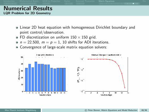
Introduction Mathematical Basics MOR by Projection RatInt Balanced Truncation Matrix Equations Fin
Numerical ResultsLQR Problem for 2D Geometry
Linear 2D heat equation with homogeneous Dirichlet boundary andpoint control/observation.FD discretization on uniform 150× 150 grid.n = 22.500, m = p = 1, 10 shifts for ADI iterations.Convergence of large-scale matrix equation solvers:
Max Planck Institute Magdeburg c© Peter Benner, Matrix Equations and Model Reduction 88/96

Introduction Mathematical Basics MOR by Projection RatInt Balanced Truncation Matrix Equations Fin
Numerical ResultsNewton-ADI vs. Newton-ADI-Gelerkin
FDM for 2D heat/convection-diffusion equations on [0, 1]2 (Lyapackbenchmarks, m = p = 1) symmetric/nonsymmetric A ∈ Rn×n,n = 10, 000.
15 shifts chosen by Penzl’s heuristic from 50/25 Ritz/harmonic Ritzvalues of A.
Computations using Intel Core 2 Quad CPU of type Q9400 at 2.66GHzwith 4 GB RAM and 64Bit-MATLAB.
Max Planck Institute Magdeburg c© Peter Benner, Matrix Equations and Model Reduction 89/96

Introduction Mathematical Basics MOR by Projection RatInt Balanced Truncation Matrix Equations Fin
Numerical ResultsNewton-ADI vs. Newton-ADI-Gelerkin
FDM for 2D heat/convection-diffusion equations on [0, 1]2 (Lyapackbenchmarks, m = p = 1) symmetric/nonsymmetric A ∈ Rn×n,n = 10, 000.
15 shifts chosen by Penzl’s heuristic from 50/25 Ritz/harmonic Ritzvalues of A.
Computations using Intel Core 2 Quad CPU of type Q9400 at 2.66GHzwith 4 GB RAM and 64Bit-MATLAB.
Newton-ADIstep rel. change rel. residual ADI
1 1 9.99e–01 2002 9.99e–01 3.41e+01 233 5.25e–01 6.37e+00 204 5.37e–01 1.52e+00 205 7.03e–01 2.64e–01 236 5.57e–01 1.56e–02 237 6.59e–02 6.30e–05 238 4.02e–04 9.68e–10 239 8.45e–09 1.09e–11 23
10 1.52e–14 1.09e–11 23
CPU time: 76.9 sec.
Newton-Galerkin-ADIstep rel. change rel. residual ADI
1 1 3.56e–04 202 5.25e–01 6.37e+00 103 5.37e–01 1.52e+00 64 7.03e–01 2.64e–01 105 5.57e–01 1.57e–02 106 6.59e–02 6.30e–05 107 4.03e–04 9.79e–10 108 8.45e–09 1.43e–15 10
CPU time: 38.0 sec.
Max Planck Institute Magdeburg c© Peter Benner, Matrix Equations and Model Reduction 89/96

Introduction Mathematical Basics MOR by Projection RatInt Balanced Truncation Matrix Equations Fin
Numerical ResultsNewton-ADI vs. Newton-ADI-Gelerkin
FDM for 2D heat/convection-diffusion equations on [0, 1]2 (Lyapackbenchmarks, m = p = 1) symmetric/nonsymmetric A ∈ Rn×n,n = 10, 000.
15 shifts chosen by Penzl’s heuristic from 50/25 Ritz/harmonic Ritzvalues of A.
Computations using Intel Core 2 Quad CPU of type Q9400 at 2.66GHzwith 4 GB RAM and 64Bit-MATLAB.
0 2 4 6 8 1010
−14
10−12
10−10
10−8
10−6
10−4
10−2
100
rela
tive
ch
an
ge
in
LR
CF
iteration index
no projection
ever step
every 5th step
0 2 4 6 8 1010
−15
10−10
10−5
100
105
rela
tive
re
sid
ua
l n
orm
iteration index
no projection
ever step
every 5th step
Max Planck Institute Magdeburg c© Peter Benner, Matrix Equations and Model Reduction 89/96

Introduction Mathematical Basics MOR by Projection RatInt Balanced Truncation Matrix Equations Fin
Numerical ResultsNewton-ADI vs. Newton-ADI-Gelerkin
FDM for 2D heat/convection-diffusion equations on [0, 1]2 (Lyapackbenchmarks, m = p = 1) symmetric/nonsymmetric A ∈ Rn×n,n = 10, 000.
15 shifts chosen by Penzl’s heuristic from 50/25 Ritz/harmonic Ritzvalues of A.
Computations using Intel Core 2 Quad CPU of type Q9400 at 2.66GHzwith 4 GB RAM and 64Bit-MATLAB.
Newton-ADIstep rel. change rel. residual ADI
1 1 9.99e–01 2002 9.99e–01 3.56e+01 603 3.11e–01 3.72e+00 394 2.88e–01 9.62e–01 405 3.41e–01 1.68e–01 456 1.22e–01 5.25e–03 427 3.88e–03 2.96e–06 478 2.30e–06 6.09e–13 47
CPU time: 185.9 sec.
Newton-Galerkin-ADIstep rel. change rel. residual ADI it.
1 1 1.78e–02 352 3.11e–01 3.72e+00 153 2.88e–01 9.62e–01 204 3.41e–01 1.68e–01 155 1.22e–01 5.25e–03 206 3.89e–03 2.96e–06 157 2.30e–06 6.14e–13 20
CPU time: 75.7 sec.
Max Planck Institute Magdeburg c© Peter Benner, Matrix Equations and Model Reduction 89/96
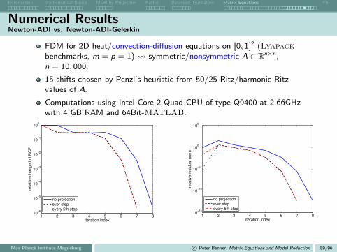
Introduction Mathematical Basics MOR by Projection RatInt Balanced Truncation Matrix Equations Fin
Numerical ResultsNewton-ADI vs. Newton-ADI-Gelerkin
FDM for 2D heat/convection-diffusion equations on [0, 1]2 (Lyapackbenchmarks, m = p = 1) symmetric/nonsymmetric A ∈ Rn×n,n = 10, 000.
15 shifts chosen by Penzl’s heuristic from 50/25 Ritz/harmonic Ritzvalues of A.
Computations using Intel Core 2 Quad CPU of type Q9400 at 2.66GHzwith 4 GB RAM and 64Bit-MATLAB.
1 2 3 4 5 6 7 810
−6
10−5
10−4
10−3
10−2
10−1
100
rela
tive c
hange in L
RC
F
iteration index
no projection
ever step
every 5th step
1 2 3 4 5 6 7 810
−15
10−10
10−5
100
105
rela
tive
re
sid
ua
l n
orm
iteration index
no projection
ever step
every 5th step
Max Planck Institute Magdeburg c© Peter Benner, Matrix Equations and Model Reduction 89/96

Introduction Mathematical Basics MOR by Projection RatInt Balanced Truncation Matrix Equations Fin
Numerical ResultsExample: LQR Problem for 3D Geometry
Control problem for 3d Convection-Diffusion Equation
FDM for 3D convection-diffusion equation on [0, 1]3
proposed in [Simoncini ’07], q = p = 1
non-symmetric A ∈ Rn×n , n = 10 648
Test system:
INTEL Xeon 5160 3.00GHz ; 16 GB RAM; 64Bit-MATLAB (R2010a) using threadedBLAS; stopping tolerance: 10−10
Max Planck Institute Magdeburg c© Peter Benner, Matrix Equations and Model Reduction 90/96
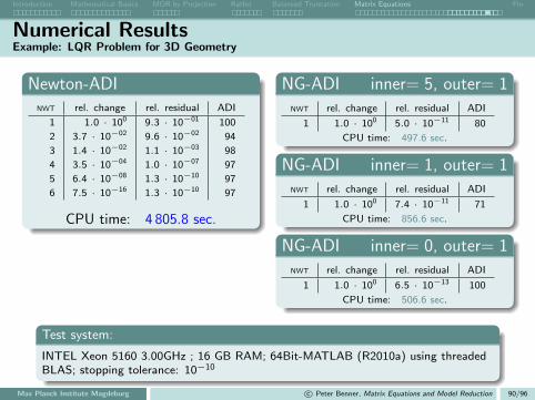
Introduction Mathematical Basics MOR by Projection RatInt Balanced Truncation Matrix Equations Fin
Numerical ResultsExample: LQR Problem for 3D Geometry
Newton-ADINWT rel. change rel. residual ADI
1 1.0 · 100 9.3 · 10−01 100
2 3.7 · 10−02 9.6 · 10−02 94
3 1.4 · 10−02 1.1 · 10−03 98
4 3.5 · 10−04 1.0 · 10−07 97
5 6.4 · 10−08 1.3 · 10−10 97
6 7.5 · 10−16 1.3 · 10−10 97
CPU time: 4 805.8 sec.
NG-ADI inner= 5, outer= 1NWT rel. change rel. residual ADI
1 1.0 · 100 5.0 · 10−11 80
CPU time: 497.6 sec.
NG-ADI inner= 1, outer= 1NWT rel. change rel. residual ADI
1 1.0 · 100 7.4 · 10−11 71
CPU time: 856.6 sec.
NG-ADI inner= 0, outer= 1NWT rel. change rel. residual ADI
1 1.0 · 100 6.5 · 10−13 100
CPU time: 506.6 sec.
Test system:
INTEL Xeon 5160 3.00GHz ; 16 GB RAM; 64Bit-MATLAB (R2010a) using threadedBLAS; stopping tolerance: 10−10
Max Planck Institute Magdeburg c© Peter Benner, Matrix Equations and Model Reduction 90/96

Introduction Mathematical Basics MOR by Projection RatInt Balanced Truncation Matrix Equations Fin
Numerical ResultsScaling of CPU times / Mesh Independence
Ω
(0, 1)
(0, 0)
(1, 1)
(1, 0)
Γc
∂tx(ξ, t) = ∆x(ξ, t) in Ω
∂νx = b(ξ) · u(t)− x on Γc
∂νx = −x on ∂Ω \ Γc
x(ξ, 0) = 1
Note:Here b(ξ) = 4 (1− ξ2) ξ2 for ξ ∈ Γc and 0 otherwise, thus ∀t ∈ R>0, wehave u(t) ∈ R.
⇒ Bh = MΓ,h · b.
Max Planck Institute Magdeburg c© Peter Benner, Matrix Equations and Model Reduction 91/96

Introduction Mathematical Basics MOR by Projection RatInt Balanced Truncation Matrix Equations Fin
Numerical ResultsScaling of CPU times / Mesh Independence
Ω
(0, 1)
(0, 0)
(1, 1)
(1, 0)
Γc
∂tx(ξ, t) = ∆x(ξ, t) in Ω
∂νx = b(ξ) · u(t)− x on Γc
∂νx = −x on ∂Ω \ Γc
x(ξ, 0) = 1
Consider: output equation y = Cx , where
C : L2(Ω) → Rx(ξ, t) 7→ y(t) =
∫Ωx(ξ, t) dξ
⇒ Ch = 1 ·Mh.
Max Planck Institute Magdeburg c© Peter Benner, Matrix Equations and Model Reduction 91/96

Introduction Mathematical Basics MOR by Projection RatInt Balanced Truncation Matrix Equations Fin
Numerical ResultsScaling of CPU times / Mesh Independence
Simplified Low Rank Newton-Galerkin ADI
generalized state space form implementation
Penzl shifts (16/50/25) with respect to initial matrices
projection acceleration in every outer iteration step
projection acceleration in every 5-th inner iteration step
Test system:
INTEL Xeon 5160 @ 3.00 GHz; 16 GB RAM; 64Bit-MATLAB (R2010a)using threaded BLAS,stopping criterion tolerances: 10−10
Max Planck Institute Magdeburg c© Peter Benner, Matrix Equations and Model Reduction 92/96

Introduction Mathematical Basics MOR by Projection RatInt Balanced Truncation Matrix Equations Fin
Numerical ResultsScaling of CPU times / Mesh Independence
Computation Times
discretization level problem size time in seconds3 81 4.87 · 10−2
4 289 2.81 · 10−1
5 1 089 5.87 · 10−1
6 4 225 2.637 16 641 2.03 · 10+1
8 66 049 1.22 · 10+2
9 263 169 1.05 · 10+3
10 1 050 625 1.65 · 10+4
11 4 198 401 1.35 · 10+5
Test system:
INTEL Xeon 5160 @ 3.00 GHz; 16 GB RAM; 64Bit-MATLAB (R2010a)using threaded BLAS,stopping criterion tolerances: 10−10
Max Planck Institute Magdeburg c© Peter Benner, Matrix Equations and Model Reduction 92/96

Introduction Mathematical Basics MOR by Projection RatInt Balanced Truncation Matrix Equations Fin
Solving Large-Scale Matrix EquationsSoftware
Lyapack [Penzl 2000]
MATLAB toolbox for solving
– Lyapunov equations and algebraic Riccati equations,
– model reduction and LQR problems.
Main work horse: Low-rank ADI and Newton-ADI iterations.
Max Planck Institute Magdeburg c© Peter Benner, Matrix Equations and Model Reduction 93/96

Introduction Mathematical Basics MOR by Projection RatInt Balanced Truncation Matrix Equations Fin
Solving Large-Scale Matrix EquationsSoftware
Lyapack [Penzl 2000]
MATLAB toolbox for solving
– Lyapunov equations and algebraic Riccati equations,
– model reduction and LQR problems.
Main work horse: Low-rank ADI and Newton-ADI iterations.
M.E.S.S. – Matrix Equations Sparse Solvers[B./Kohler/Saak ’08–]
Extended and revised version of Lyapack.
Includes solvers for large-scale differential Riccati equations (based onRosenbrock and BDF methods).
Many algorithmic improvements:
– new ADI parameter selection,– column compression based on RRQR,– more efficient use of direct solvers,– treatment of generalized systems without factorization of the mass matrix,– new ADI versions avoiding complex arithmetic etc.
C and MATLAB versions.
Max Planck Institute Magdeburg c© Peter Benner, Matrix Equations and Model Reduction 93/96
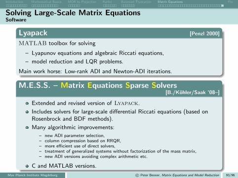
Introduction Mathematical Basics MOR by Projection RatInt Balanced Truncation Matrix Equations Fin
Solving Large-Scale Matrix EquationsSoftware
Lyapack [Penzl 2000]
MATLAB toolbox for solving
– Lyapunov equations and algebraic Riccati equations,
– model reduction and LQR problems.
Main work horse: Low-rank ADI and Newton-ADI iterations.
M.E.S.S. – Matrix Equations Sparse Solvers[B./Kohler/Saak ’08–]
Extended and revised version of Lyapack.
Includes solvers for large-scale differential Riccati equations (based onRosenbrock and BDF methods).
Many algorithmic improvements:
– new ADI parameter selection,– column compression based on RRQR,– more efficient use of direct solvers,– treatment of generalized systems without factorization of the mass matrix,– new ADI versions avoiding complex arithmetic etc.
C and MATLAB versions.
Max Planck Institute Magdeburg c© Peter Benner, Matrix Equations and Model Reduction 93/96

Introduction Mathematical Basics MOR by Projection RatInt Balanced Truncation Matrix Equations Fin
Topics Not Covered
Extensions to bilinear and stochastic systems.
Rational interpolation methods for nonlinear systems.
Other MOR techniques like POD, RB.
MOR methods for discrete-time systems.
Extensions to descriptor systems Ex = Ax + Bu, E singular.
Parametric model reduction:
x = A(p)x + B(p)u, y = C (p)x ,
where p ∈ Rd is a free parameter vector; parameters should bepreserved in the reduced-order model.
Max Planck Institute Magdeburg c© Peter Benner, Matrix Equations and Model Reduction 94/96

Introduction Mathematical Basics MOR by Projection RatInt Balanced Truncation Matrix Equations Fin
Further Reading — Model Order Reduction
1 G. Obinata and B.D.O. Anderson.Model Reduction for Control System Design.Springer-Verlag, London, UK, 2001.
2 Z. Bai.Krylov subspace techniques for reduced-order modeling of large-scale dynamical systems.Appl. Numer. Math, 43(1–2):9–44, 2002.
3 R. Freund.Model reduction methods based on Krylov subspaces.Acta Numerica, 12:267–319, 2003.
4 P. Benner, E.S. Quintana-Ortı, and G. Quintana-Ortı.State-space truncation methods for parallel model reduction of large-scale systems.Parallel Comput., 29:1701–1722, 2003.
5 P. Benner, V. Mehrmann, and D. Sorensen (editors).Dimension Reduction of Large-Scale Systems.Lecture Notes in Computational Science and Engineering, Vol. 45,Springer-Verlag, Berlin/Heidelberg, Germany, 2005.
6 A.C. Antoulas.Lectures on the Approximation of Large-Scale Dynamical Systems.SIAM Publications, Philadelphia, PA, 2005.
7 P. Benner, R. Freund, D. Sorensen, and A. Varga (editors).Special issue on Order Reduction of Large-Scale Systems.Linear Algebra Appl., June 2006.
8 W.H.A. Schilders, H.A. van der Vorst, and J. Rommes (editors).Model Order Reduction: Theory, Research Aspects and Applications.Mathematics in Industry, Vol. 13,Springer-Verlag, Berlin/Heidelberg, 2008.
9 P. Benner, J. ter Maten, and M. Hinze (editors).Model Reduction for Circuit Simulation.Lecture Notes in Electrical Engineering, Vol. 74,Springer-Verlag, Dordrecht, 2011.
Max Planck Institute Magdeburg c© Peter Benner, Matrix Equations and Model Reduction 95/96

Introduction Mathematical Basics MOR by Projection RatInt Balanced Truncation Matrix Equations Fin
Further Reading — Matrix Equations
1 V. Mehrmann.The Autonomous Linear Quadratic Control Problem, Theory and Numerical Solution.Number 163 in Lecture Notes in Control and Information Sciences. Springer-Verlag, Heidelberg, July 1991.
2 P. Lancaster and L. Rodman.The Algebraic Riccati Equation.Oxford University Press, Oxford, 1995.
3 P. Benner.Computational methods for linear-quadratic optimizationRendiconti del Circolo Matematico di Palermo, Supplemento, Serie II, 58:21–56, 1999.
4 T. Penzl.Lyapack Users Guide.Technical Report SFB393/00-33, Sonderforschungsbereich 393 Numerische Simulation auf massiv parallelen Rechnern, TUChemnitz, 09107 Chemnitz, FRG, 2000.Available from http://www.tu-chemnitz.de/sfb393/sfb00pr.html.
5 H. Abou-Kandil, G. Freiling, V. Ionescu, and G. Jank.Matrix Riccati Equations in Control and Systems Theory.Birkhauser, Basel, Switzerland, 2003.
6 P. Benner.Solving large-scale control problems.IEEE Control Systems Magazine, 24(1):44–59, 2004.
7 D. Bini, B. Iannazzo, and B. Meini.Numerical Solution of Algebraic Riccati Equations.SIAM, Philadelphia, PA, 2012.
8 P. Benner and J. Saak.Numerical solution of large and sparse continuous time algebraic matrix Riccati and Lyapunov equations: a state of the artsurvey.GAMM-Mitteilungen, 36(1):32-–52, 2013.
9 V. Simoncini.Computational methods for linear matrix equations (survey article).March 2013.http://www.dm.unibo.it/~simoncin/matrixeq.pdf.
Max Planck Institute Magdeburg c© Peter Benner, Matrix Equations and Model Reduction 96/96


