Measurement for Improvement

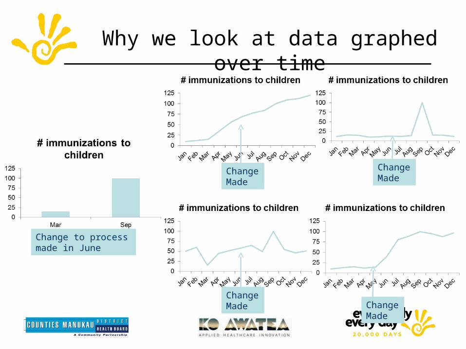
Why we look at data graphed over time
Change Made
Change Made
Change Made Change
Made
Change to process made in June

Improvement Science Consulting
O1
P1
Measure Types
O = Outcome Measure
P = Process Measure
B = Balance Measure
S = Process Step Measure
PDSA = Learning Cycle Measure
O2
P2
B B
P1 P2
S3S2S1
System of Feedback
PDSA1
PDSA2
PDSA3
PDSA4
S3S2S1
PDSA1
PDSA2
PDSA3
PDSA4
© Improvement Science Consulting

Break out – developing a useful project level dashboard
• Spend some time developing the measures you would like to include in a project level dashboard
• Which ones are outcome measures?• Which ones are process measures?• Do you have balance measures?• Process step measures?
• Note any gaps in your measures – where would you like to add measures?

Improvement Science Consulting
O1
P1
Measure Types
O = Outcome Measure
P = Process Measure
B = Balance Measure
S = Process Step Measure
PDSA = Learning Cycle Measure
O2
P2
B B
P1 P2
S3S2S1
System of Feedback
PDSA1
PDSA2
PDSA3
PDSA4
S3S2S1
PDSA1
PDSA2
PDSA3
PDSA4
© Improvement Science Consulting

As the scale of the test increases we move from qualitative to quantitative evidence
Improvement Science Consulting
Very small scale test of
a change idea
Large scale test of change idea or
Implementation of a change idea
Evidence primarily
Qualitative
Evidence primarily Quantitative with
noticeable impact on process measures
Sequence of learning and change

Run Charts
Making and Interpreting

So what is a run chart?
Murray and Provost, Pg 3-4
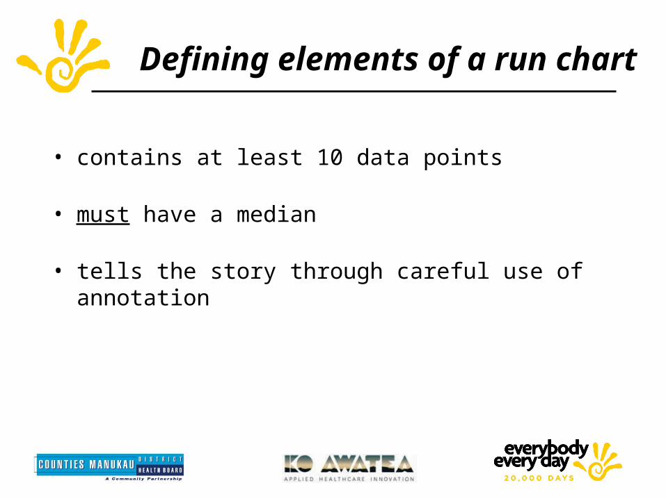
Defining elements of a run chart
• contains at least 10 data points
• must have a median
• tells the story through careful use of annotation

What time is it?
• Stop what you are doing
• Look at your watch
• Write down the time
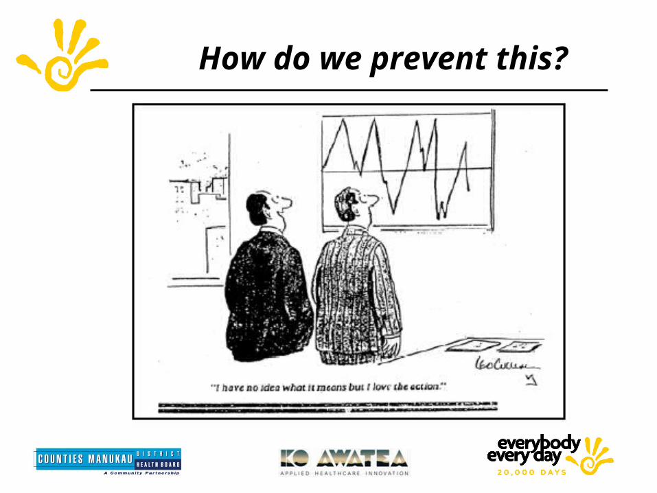
How do we prevent this?
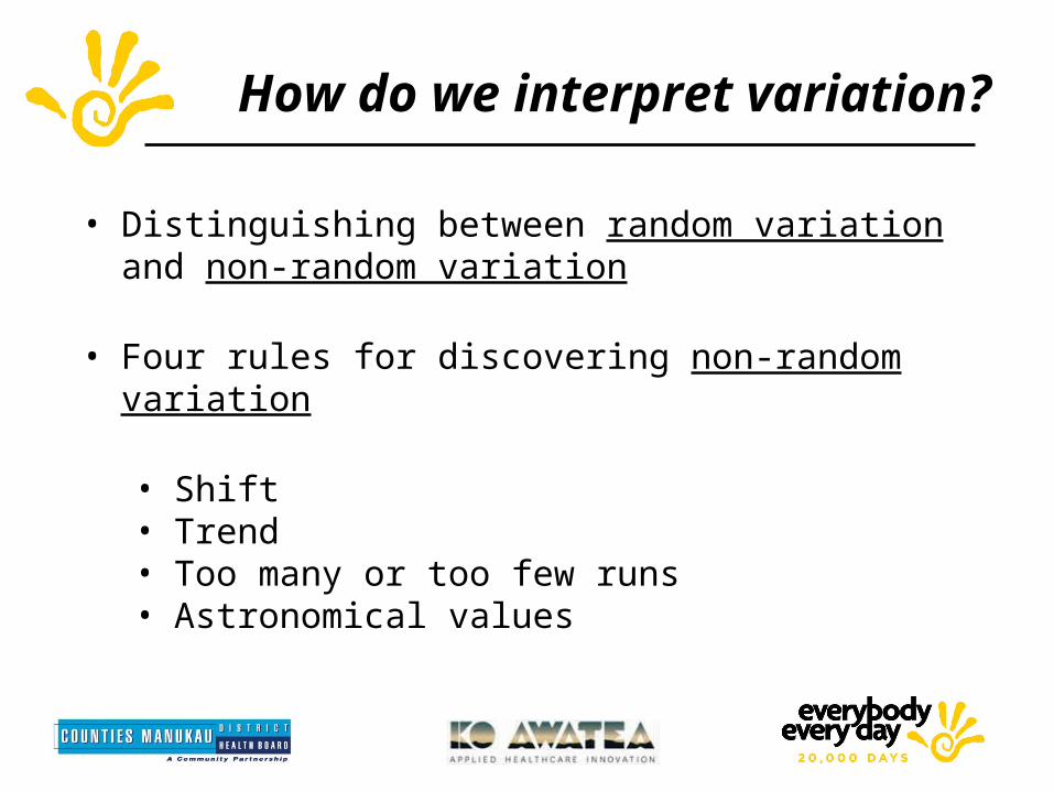
How do we interpret variation?
• Distinguishing between random variation and non-random variation
• Four rules for discovering non-random variation
• Shift• Trend• Too many or too few runs• Astronomical values
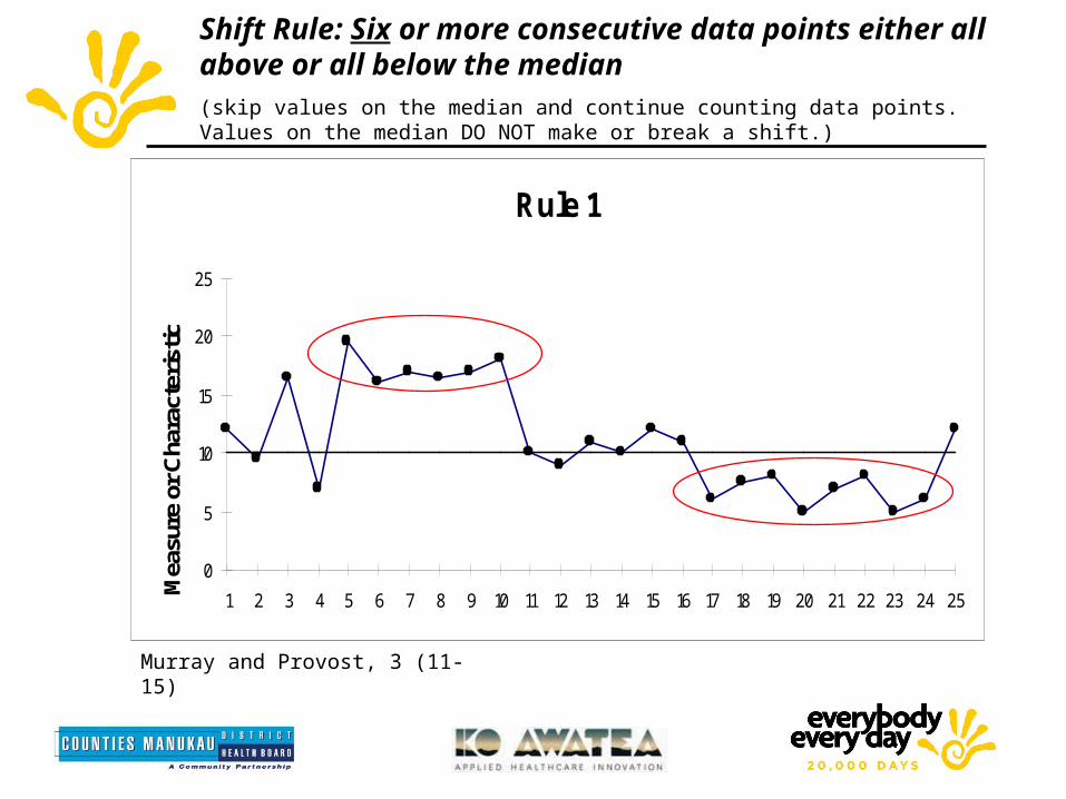
Shift Rule: Six or more consecutive data points either all above or all below the median (skip values on the median and continue counting data points. Values on the median DO NOT make or break a shift.)
Rule 1
0
5
10
15
20
25
1 2 3 4 5 6 7 8 9 10 11 12 13 14 15 16 17 18 19 20 21 22 23 24 25Mea
sure
or C
hara
cter
istic
Murray and Provost, 3 (11-15)

Why do we need 6 data points?
What is the probability of a coin landing heads or tails?
.5.5 x .5 = .25.5 x .5 x .5 = .125.5 x .5 x .5 x .5 = .0625.5 x .5 x .5 x .5 x .5 = .03125.5 x .5 x .5 x .5 x .5 x .5 = .015625

Trend Rule: Five or more consecutive data points either all going up or all going down. (If the value of two or more consecutive points is the same, ignore one of the points when counting; like values do not make or break a trend.)
Murray and Provost, 3 (11-15)
Rule 2
0
5
10
15
20
25
1 2 3 4 5 6 7 8 9 10 11 12 13 14 15 16 17 18 19 20 21 22 23 24 25
Mea
sure
or C
hara
cter
istic
Median=11

Run Rule: Too many or too few runs (A run is a series of points in a row on one side of the median. Some points fall right on the median, which makes it hard to decide which run these points belong to. So, an easy way to determine the number of runs is to count the number of times the data line crosses the median and add one. Statistically significant change signaled by too few or too many runs).
Murray and Provost, 3 (11-15)
Rule 3
0
5
10
15
20
25
1 2 3 4 5 6 7 8 9 10
Measure
or C
hara
ceristic
Median 11.4
10 Data points not on medianData line crosses onceToo few runs: total 2 runs
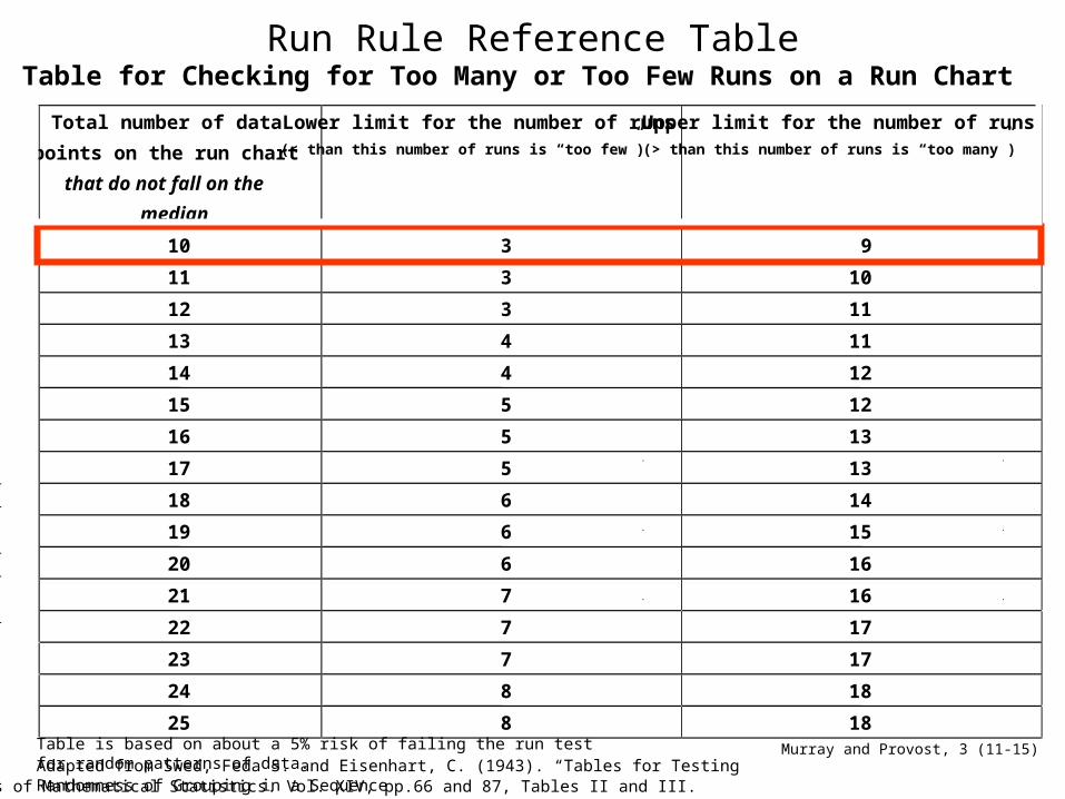
Run Rule Reference TableTable for Checking for Too Many or Too Few Runs on a Run Chart
Total number of data
points on the run chart
that do not fall on the
median
Lower limit for the number of runs(< than this number of runs is “too few”)
Upper limit for the number of runs(> than this number of runs is “too many”)
10 3 9
11 3 10
12 3 11
13 4 11
14 4 12
15 5 12
16 5 13
17 5 13
18 6 14
19 6 15
20 6 16
21 7 16
22 7 17
23 7 17
24 8 18
25 8 18Table is based on about a 5% risk of failing the run test for random patterns of data.Adapted from Swed, Feda S. and Eisenhart, C. (1943). “Tables for Testing Randomness of Grouping in a Sequence
of Alternatives. Annals of Mathematical Statistics. Vol. XIV, pp.66 and 87, Tables II and III.
Murray and Provost, 3 (11-15)
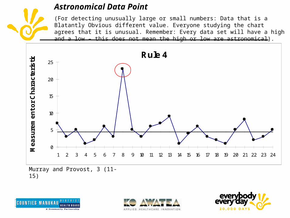
Astronomical Data Point (For detecting unusually large or small numbers: Data that is a Blatantly Obvious different value. Everyone studying the chart agrees that it is unusual. Remember: Every data set will have a high and a low – this does not mean the high or low are astronomical).
Murray and Provost, 3 (11-15)
Rule 4
0
5
10
15
20
25
1 2 3 4 5 6 7 8 9 10 11 12 13 14 15 16 17 18 19 20 21 22 23 24
Measure
ment or C
hara
cte
ristic
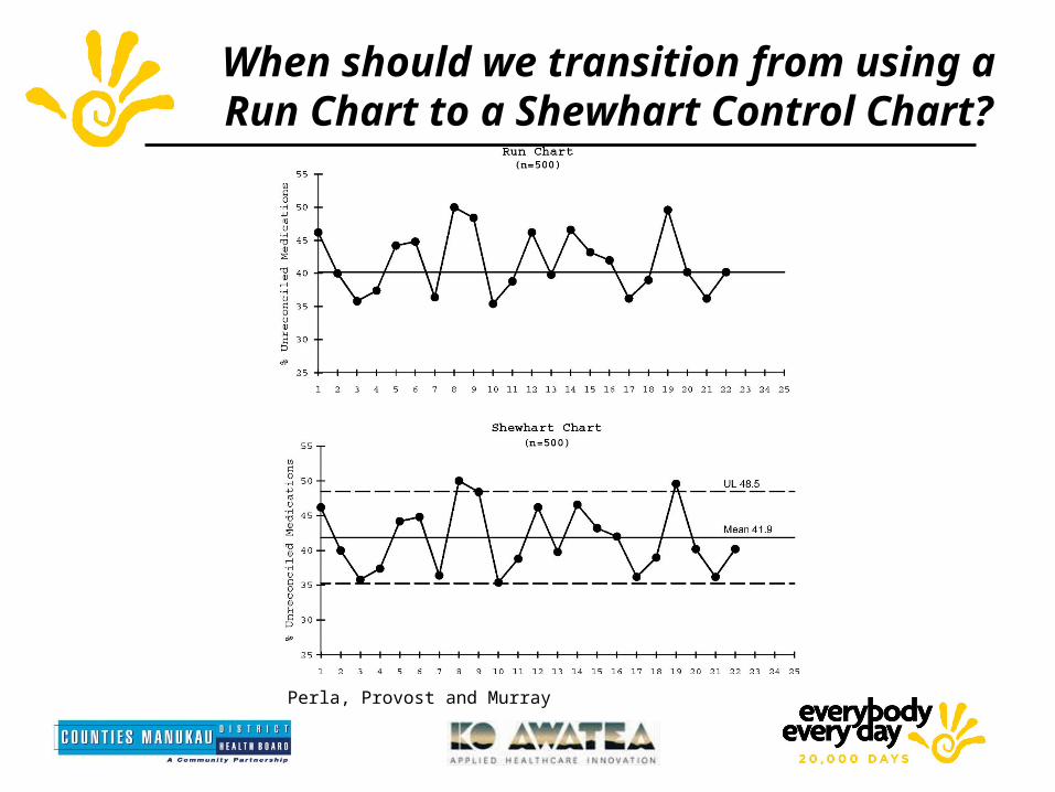
When should we transition from using a Run Chart to a Shewhart Control Chart?
Perla, Provost and Murray


