
Measurement of Propeller Lift Force
Lab 2 Final Report
VM495 Mechanical Engineering Laboratory II
Fall 2015
Project Duration:
October 20th, 2015 — Dec 16th, 2015
Project Submission Date:
Dec 16th, 2015
Prepared by:
Chennan Li
Junjie Shen
Mo Chen
Yang Shen
Undergraduate Mechanical Engineering Students
UM-SJTU Joint Institute
Team 1D
Prepared for:
Dr. David L.S. Hung
Associate Professor, VM495 Engineering Instructor
UM-SJTU Joint Institute
Dr. Kwee-Yan Teh
Assistant Researcher & Lecturer, VM495 Technical Communication Instructor
UM-SJTU Joint Institute


Abstract
The increasing use of Small Unmanned Aerial Vehicle (SUAV, such as quadrotor) has
triggered the interest in analyzing the performance of the motor(s) mounted with the
propeller(s) that power them. The objective of this experiment is to measure the lift
force of a single propeller under static condition, find out its relation with the rotating
speed (Test 1), and study the effect of wind shield located under the rotating propeller
(Test 2) as well as the vibration of unbalanced propellers (Test 3). For Test 1, the
experimental results show that when the propeller was rotating under static condition
(zero flight speed), the lift force it generated was proportional to the square of its
rotating speed. Furthermore, at the same rotating speed, the propeller with larger
diameter, larger pitch, and more blades would generate larger lift force. For Test 2, the
wind shield, with larger area and smaller distance under the propeller, would increase
the propeller lift force. For Test 3, more unbalance of the propeller would result in larger
vibration. However, it is difficult to well quantify the unbalance. Finally, with good
repeatability, the data collected in this experiment and the self-made measuring device
can be used to verify whether the SUAV is able to accomplish the proposed mission
with the target motor(s) and propeller(s).


Table of Content
1. INTRODUCTION .................................................................................................. 1
2. TEST OBJECTIVE ................................................................................................. 2
2.1 TEST 1 - EFFECT OF PROPELLER DIAMETER, PITCH, AND BLADE NUMBER............ 3
2.2 TEST 2 - EFFECT OF WIND SHIELD UNDER PROPELLER .......................................... 3
2.3 TEST 3 - VIBRATION OF UNBALANCED PROPELLERS ............................................. 4
3. EXPERIMENTAL SETUP ..................................................................................... 4
3.1 MECHANICAL SETUP ............................................................................................. 4
3.1.1 Load Cell Fixture ........................................................................................... 6
3.1.2 Motor Fixture ................................................................................................. 7
3.2 ELECTRICAL SETUP ............................................................................................... 8
3.2.1 Motor Connection .......................................................................................... 8
3.2.2 KV Value ......................................................................................................... 9
4. SENSORS ............................................................................................................... 9
4.1 PHOTO DETECTOR ................................................................................................. 9
4.1.1 Sensitivity ..................................................................................................... 10
4.1.2 Data Processing ........................................................................................... 10
4.2 LOAD CELL ......................................................................................................... 12
4.2.1 Test Experiment ............................................................................................ 13
4.2.2 Calibration ................................................................................................... 14
4.2.3 Data Processing ........................................................................................... 16
5. RESULTS & DICUSSION ................................................................................... 17
5.1 TEST 1 - EFFECT OF PROPELLER DIAMETER, PITCH, AND BLADE NUMBER.......... 19
5.2 TEST 2 - EFFECT OF WIND SHIELD UNDER PROPELLER ........................................ 21
5.3 TEST 3 - VIBRATION OF UNBALANCED PROPELLERS ........................................... 22
6. COST & SCHEDULE .......................................................................................... 24
6.1 BILL OF MATERIALS ............................................................................................ 24
6.2 FINAL SCHEDULE ................................................................................................ 24
7. CONCLUSION ..................................................................................................... 25
REFERENCES ............................................................................................................ 27
APPENDIX A: TEST RESULTS ............................................................................... A-1
APPENDIX B: CALIBRATION DATA .................................................................... B-1
APPENDIX C: MATLAB CODE .............................................................................. C-1
APPENDIX D: LABVIEW PROGRAM ................................................................... D-1
APPENDIX E: EQUIPMENT AND MATERIALS .................................................. E-1
APPENDIX F: AUTOCAD DRAWING ................................................................... F-1


1
1. INTRODUCTION
Quadrotor is a type of Small Unmanned Aerial Vehicle (SUAV). It has been becoming
more and more popular all over the world due to its excellent motion performance. It
can not only adapt to complex terrains but also accomplish difficult flight missions.
With modules of various functions, quadrotor has great potential in many fields, such
as search and rescue, prospection of zone of ignorance and monitor of public territory.
The realization of the latest control algorithm allows the quadrotor to resist large
excitation with high accuracy. Figure 1.1 shows the free body diagram of a typical
quadrotor.
Figure 1.1: Free body diagram of the quadrotor. Retrieved from
http://www.mathworks.com/matlabcentral/answers/109279-modelling-a-quadrotor-
with-simmechanics.
Propellers provide the thrust force (also known as lift force under static condition) for
many of these SUAVs and the magnitude of the thrust force is largely dependent on the
propeller characteristics (such as diameter, pitch, blade number, etc.), the rotating speed
of the propeller, and the flight speed (indicated as u in Figure 1.1).[1] Since the small-
scale propellers have relatively small thrust coefficient and low efficiency, current
research focuses on the improvement of these two parameters.

2
2. TEST OBJECTIVE
The objective of this experiment is to measure the lift force of a single propeller uner
static condition, find out its relation with the rotating speed, and study the effect of the
wind shield located under the rotating propeller as well as the vibration of unbalanced
propellers. At the beginning, a particular measuring fixture was designed and fabricated.
It combined a photo detector (to measure the motor speed), a load cell (to measure the
force), a brushless motor mounted with the test propeller, and a detachable wind shield.
Algorithm for the photo detector and calibration for the load cell were then carried out
to obtain the final results, e.g., the rotating speed and corresponding lift force.
For Test 1, pitch is defined as the displacement a propeller makes in a complete spin of
360° angle, shown in Figure 2.1.[3]
Figure 2.1: Pitch.[3]
For Test 2, Figure 2.2 shows the wind shield. Note that each block has an angle of 45°.
Figure 2.2: Wind shield.

3
For Test 3, Figure 2.3 shows a balanced propeller. Figure 2.4 shows an unbalanced
propeller due to wear. Figure 2.5 shows an unbalanced propeller due to wear and cut.
Figure 2.3: Balanced propeller.
Figure 2.4: Unbalanced propeller due to wear.
Figure 2.5: Unbalanced propeller due to wear and cut.
2.1 Test 1 - Effect of Propeller Diameter, Pitch, and Blade Number
Step 1: Assemble the experimental setup and check whether the brushless motor work
normally.
Step 2: Install the propeller and check whether the propeller is well assembled.
Step 3: Rotate the adjusting knob to 10 fixed values. For each value, record the data of
photo detector and load cell through NI myDAQ. The number of data is 8192
(= 213) for each sensor and for each value.
Step 4: Change the propeller with different characteristics (diameter, pitch, and blade
number) and redo step 3.
2.2 Test 2 - Effect of Wind Shield under Propeller
Step 1: Assemble the wind shield with no piece on it.
Step 2: Install the propeller and check whether the propeller is well assembled.
Step 3: Rotate the adjusting knob to a certain value and record the data of photo
detector and load cell through NI myDAQ.
Step 4: Assemble one block on the wind shield and record the data of photo detector
and load cell through NI myDAQ.
Step 5: Assemble another block on the wind shield and redo step 4 until all 8 blocks
assembled on the wind shield.

4
Step 6: Change four different distances between the wind shield and propeller. For each
time, record the data of photo detector and load cell through NI myDAQ.
2.3 Test 3 - Vibration of Unbalanced Propellers
Step 1: Assemble a balanced propeller and record the data of photo detector and load
cell through NI myDAQ..
Step 2: Wear the propeller (Figure 2.4) and record the data of photo detector and load
cell through NI myDAQ.
Step 3: Further cut a small part of the propeller (Figure 2.5) and record the data of
photo detector and load cell through NI myDAQ.
3. EXPERIMENTAL SETUP
Figure 3.1 shows the entire experimental setup. In particular, it consists of two main
parts. One is the mechanical setup and the other is the electrical setup.
Figure 3.1: Experimental setup.
3.1 Mechanical Setup
Figure 3.2 shows the mechanical setup design. The yellow component is the photo
detector (which we borrow from the Mechanical Lab), the black component is the
brushless motor, and the brown component below is the load cell we bought. The design

5
was carried out in SolidWorks, aiming to clearly demonstrate the design itself, as well
as to verify that the dimensions of all the components could make the setup work for
different motors and propellers. Note that the mobility is quite important for this
experiment, shown in Figure 3.3.
Figure 3.2: Experimental setup design.
Figure 3.3: Experimental setup mobility.
Figure 3.4 shows the mechanical setup we fabricated. The main material we used is
acryl since it is easy to fabricate as well as has enough strength. We first translated the
3D SolidWorks file into 2D AutoCAD file. With the help of Mr. Chen Tianhua, we then
used the laser cutting machine to obtain each component. Later, we assembled the entire
mechanical setup with auxiliary materials, such as bolts, nuts, columns, etc. It turned
out that the design met the experimental requirements.

6
Figure 3.4: Mechanical setup.
3.1.1 Load Cell Fixture
As shown in Figure 3.5, the load cell we bought had thread at both ends. Therefore, we
used three layers of acrylic boards, with the middle one left a space for an M5 nut, to
fix the load cell, shown in Figure 3.6. The upper end was applied the same method.
Figure 3.5: Load cell with thread at both ends.

7
Figure 3.6: Load cell fixture.
3.1.2 Motor Fixture
The modified design was to connect the motor and the load cell with bolts and acrylic
boards instead of a string. However, when the motor mounted with the propeller was
rotating, it created a torque as well as a lift force. So in order to balance the torque, we
used four columns to prevent the rotation of the motor, shown in Figure 3.7. The fixture
only allowed vertical motion, which was exactly what we wanted.
Figure 3.7: Motor fixture.

8
3.2 Electrical Setup
The electrical setup is shown in Figure 3.8. No.1 component is the Lithium battery
which can provide 11.1V voltage. This Li battery could supply power for every
electrical component. No.2 component is ESC (Electric Speed Control) which is used
to control the rotating speed of the brushless motor by changing the voltage across it.
No.3 component is the brushless motor which is used to drive the propeller. No.4
component is the adjusting knob which could send pulse signal to ESC and ESC would
change the voltage across the motor accordingly.
Figure 3.8: Electrical setup.
3.2.1 Motor Connection
The brushless motor was connected to ESC. Since the brushless motor worked on three-
phase alternating current, it required three lines to connect with each other, as shown in
Figure 3.9. The middle black wire of the brushless motor was connected with the middle
wire of ESC. The other two wires of the motor were connected with the other two wires
of ESC. If you want to change the direction of rotation, you can exchange the
connection of these two wires.
Figure 3.9: Connection between the motor and ESC.

9
3.2.2 KV Value
Figure 3.10 shows the three types of motors we used in this experiment. Each of them
had different KV values. KV value is defined as the theoretical RMP the motor can
rotate per voltage input. Therefore, the theoretical RPM of a motor under certain voltage
is determined by
RPM KV Value Input Voltage . (2.1)
Hence, under the same voltage, the higher KV value will result in higher RPM; however,
higher RPM will lead to lower torque. Therefore, when we used the motor with large
KV value, we chose small-size propeller; otherwise, no lift force would be expected.
KV 880 KV 1250 KV 2400
Figure 3.10: Three motors with different KV values.
4. SENSORS
4.1 Photo Detector
We used photo detector to measure the rotating speed of the propeller. Specifically, we
recorded the output signal to monitor the passing of the propeller blade through the
photo detector. In addition to the general introduction of the photo detector, this part
includes the sensitivity of the photo detector and methodology to obtain the RPM. The
detailed characteristics of the photo detector are listed in Table 4.1.
Table 4.1: Photo detector characteristics.
Type E3S-GS3E4
Sensing Distance 30 mm
Voltage Supply 12 ~ 24 V
Response Time 1 ms
10
4.1.1 Sensitivity
Since we need to measure the RPM of the propeller, we require a relative high
sensitivity of the photo detector to catch each resolution. Our photo detector can record
signal one times per millisecond. Therefore, the theoretical maximum RPM it can
measure is given by
max 3
2 1 60 60000RPM
10 2n n
, (4.1)
where n donates the number of blades.
4.1.2 Data Processing
Initially, we wanted to calculate RPM in a simple and direct way, which was recording
the times N that the propeller passed the photo detector in 1 second and the RPM is thus
given by
RPM 60.N (4.2)
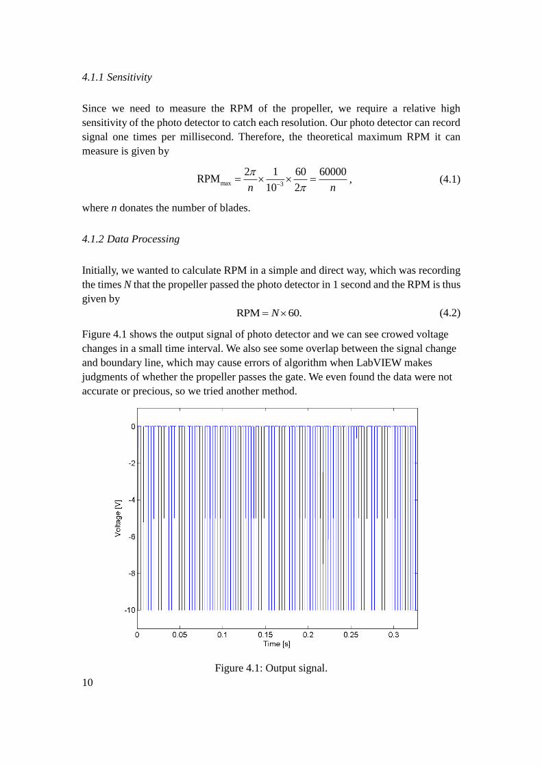
Figure 4.1 shows the output signal of photo detector and we can see crowed voltage
changes in a small time interval. We also see some overlap between the signal change
and boundary line, which may cause errors of algorithm when LabVIEW makes
judgments of whether the propeller passes the gate. We even found the data were not
accurate or precious, so we tried another method.
Figure 4.1: Output signal.

11
In the second method, in order to make sure of high accuracy, we recorded the time
interval t between 2 voltage changes, shown in Figure 4.2. For an n-blade propeller, one
signal change means the propeller goes through a semicircle. Then it takes n·t time to
make a full circle and thus the rotating speed of the propeller can be calculated by
60RPM .
n t
(4.3)
where n donates the number of blades.
Figure 4.2: Output signal in time interval 2t.
The RPM calculated by this method was correct and accurate theoretically. The
numerical value of t was around 10-3 s, which was extremely small. Therefore, a little
error of t would lead to a large difference of RPM, which means a relative large
uncertainty of RPM would occur in this method. To avoid this, we tried another method,
which is FFT.
In the last method, we used FFT to get an accurate value of RPM with a relative small
uncertainty compared to previous methods. As shown in Figure 4.3, the first peak
represents the FFT constant C0 and the second peak is the fundamental frequency f0.
Note that for a certain RPM, we take 8192 (= 213) data for calculation and the
sampling rate is 20 kHz.

12
Figure 4.3: FFT of output signal.
Therefore, the rotating speed can be determined by
0
60RPM ,f
n (4.4)
where n donates the number of blades.
4.2 Load Cell
Since our object is to find out the relationship between the lift force and the propeller
rotating speed, we have a high requirement for the range and the resolution of the load
cell. Overall, we want to find a load cell with the following characters: proper range,
small size, high resolution, fine stability and easy installation.
After consulting the engineers in the lab and owner of TaoBao, we got the general data
for a motor that, if mounted a 10’’ propeller, the lift force would achieve 600 g when
the rotating speed was around 8000 RPM. Considering the fact that in the experiment,
the size of the propeller varied from 5’’ to 10’’, we decided to choose a load cell with
capacity ±2 kg. The detailed parameters are listed in Table 4.2.
Table 4.2: Load cell characteristics.
Type BSLM-3
Capacity ±2 kg

13
Rated Output 1.5 mV/V
Non-Linearity ±0.1% FS
Zero Balance ±0.1% FS
Hysteresis ±0.1% FS
Creep (in 30 minutes) ±0.05% FS
Repeatability ±0.1% FS
4.2.1 Test Experiment
The load cell could be easily installed into the fixture, and then we started to test the
actual using condition. In the first trial, the results were horrible, shown in Figure 4.4.
Noises greatly disturbed the normal output voltage, making us really difficult to tell
what the exact output voltage was. The normal input voltage in the lab was around 10
V; hence the expected maximum output voltage was only around 15 mV. The output
results were then greatly affected by the noises. Hence, we decided to design an
amplifying circuit to increase the output voltage as well as to reduce the noise effect.
Figure 4.4: Load cell output without the amplifying circuit.
Figure 4.5 shows the designed amplifying circuit, with R1 = 815 kΩ, R2 = 217 Ω, R3 =
803 kΩ, and R4 = 218.3 Ω. By substituting them into Equation (4.5):
1
2
out
in
V R
V R , (4.5)
we can derive that the output voltage of the load cell was increased by about 3755 times,
which is exactly what we desired.
14
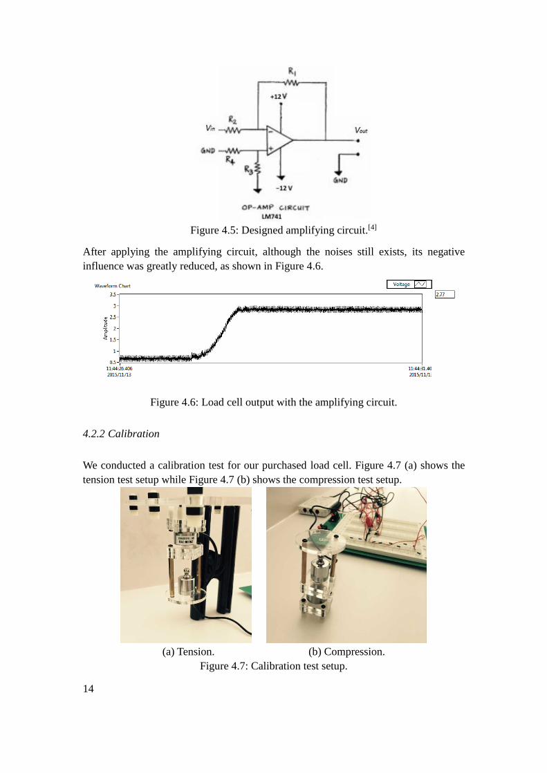
Figure 4.5: Designed amplifying circuit.[4]
After applying the amplifying circuit, although the noises still exists, its negative
influence was greatly reduced, as shown in Figure 4.6.
Figure 4.6: Load cell output with the amplifying circuit.
4.2.2 Calibration
We conducted a calibration test for our purchased load cell. Figure 4.7 (a) shows the
tension test setup while Figure 4.7 (b) shows the compression test setup.
(a) Tension. (b) Compression.
Figure 4.7: Calibration test setup.

15
The test methodology was that we recorded the output voltage of the load cell for every
50-gram increase in the weight, starting from the free-of-weight condition (but the shelf
structure, used to place the weight, was still mounted) to the maximum weight our
propellers can lift. Figure 4.8 shows the calibration result. As we can see, although we
have already taken the weight of the shelf structure into consideration, there still exists
a zero error, meaning that the output voltage of the load cell is not zero when it is free
of any load. And this zero error depends on the direction of the load cell. Note that in
Figure 4.7, the direction of the load cell in the tension test setup was opposite to that in
the compression test setup. Besides, the calibration result was quite good. We can
conclude that the output voltage of the load cell linearly depends on the load acted on
it.
Figure 4.8: Calibration test result.
Note that for every data point shown in Figure 4.8, we actually recorded 20 times,
shown in Figure 4.9. As we can see, the fluctuation was within 30 mV, indicating a 0.39%
error for this data, which is quite acceptable.

16
Figure 4.9: Output voltage for 1038-gram tension.
4.2.3 Data Processing
Figure 4.10 shows the transient step response of the load cell. Before the propeller was
rotating, the fluctuation due to noise was only about ±10 mV. However, when the
propeller was rotating, the fluctuation due to vibration was around ±200 mV, almost 20
times the initial value. Therefore, at a certain rotating speed, we recorded 8192 (= 213)
voltage data, converted them into force according to the calibration, and finally treated
the mean value as the corresponding lift force. For each propeller, lift force was
measured at 10 different rotating speeds.
Figure 4.10: Transient step response.

17
5. RESULTS & DICUSSION
The nomenclature of the propeller is important for understanding the results. For a 2-
9×6E, the blade number is 2, the diameter is 9 inches, and the pitch is 6 inches. Pitch is
defined as the displacement a propeller makes in a complete spin of 360° angle in a
solid environment.[3] Note that in a liquid environment, the propeller will slide with less
displacement. Figure 5.1 shows the relationship between the rotating speed and
corresponding lift force for the 2-9×6E propeller, with a quadratic polynomial fitting.
As we can see, the fitting result is quite good, which indicates that the propeller lift
force is proportional to the square of the rotating speed at zero flight speed.
Figure 5.1: Lift force vs. rotating speed.
To verify the confidence in the measurement, a repeatability test were carried out. In
particular, we conducted three tests for each of the propeller on three different days, as
shown in Figure 5.2. As we can see, the three curves almost overlap with each other,
which indicates that the measurement is repeatable. Other propeller repeatability test
results are shown in Appendix A.

18
Figure 5.2: Repeatability test results.
For a more general perspective, the performance of a propeller is given in term of the
lift coefficient, defined as
2 4L
LC
n D , (5.1)
where L is the lift force, ρ is the air density, n is the rotating speed, and D is the propeller
diameter[1]. Figure 5.3 shows the relationship between the rotating speed and
corresponding lift coefficient for the 2-9×6E propeller. We can see that the lift
coefficient is almost independent of the rotating speed, which makes sense. We have
previously verified that there is a quadratic relationship between the rotating speed and
corresponding lift force. With Equation (5.1), the lift coefficient is thus a constant for a
certain propeller.

19
Figure 5.3: Lift coefficient vs. rotating speed.
5.1 Test 1 - Effect of Propeller Diameter, Pitch, and Blade Number
Figure 5.4 shows the effect of propeller diameter, pitch, and blade number on lift force.
The experimental results show that when the propeller was rotating at the same rotating
speed, the propeller with larger diameter, larger pitch, and more blades would generate
larger lift force.

20
Figure 5.4: Effect of propeller diameter, pitch, and blade number on lift force.
Figure 5.5 shows the effect of propeller diameter, pitch, and blade number on lift
coefficient. As we can see, the propeller with larger pitch, and more blades would have
larger lift coefficient. However, the difference in the propeller diameter did not result
in too much change in the lift coefficient. More detailed figures are presented in
Appendix A.
Figure 5.5: Effect of propeller diameter, pitch, and blade number on lift coefficient.

21
5.2 Test 2 - Effect of Wind Shield under Propeller
Figure 5.6 shows the effect of wind shield angle on lift force. For this test, the test
propeller was 2-9×6E. The rotating speed was around 9000 RPM. The distance between
the wind shield and the propeller was fixed at 9 mm. As we can see, when the angle
was smaller than 180°, the lift force did not change too much. However, when the angle
was larger than 180°, the lift force would increase monotonously. The reason lies in the
fact that a propeller works under Newton’s Third Law and a solid base would typically
generate a larger reaction force than air. Air would just diffuse it.
Figure 5.6: Effect of wind shield angle on lift force.
Figure 5.7 shows the effect of distance between the wind shield and the propeller. For
this test, the test propeller was still 2-9×6E. The rotating speed was also around 9000
RPM while the wind shield angle was fixed at 360°. Due to the limitation of the
mechanical setup, we could only obtained 4 data points. However, the trend is obvious.
With larger distance between the wind shield and the propeller, the lift force would
decrease.

22
Figure 5.7: Effect of distance between the wind shield and the propeller on lift force.
5.3 Test 3 - Vibration of Unbalanced Propellers
Propellers, after long-time service, may experience damage due to both wear and cut.
For this test, we tested the same 2-9×6E propeller at the same rotating speed (around
9000 RPM) but under different conditions. The first was the balanced condition. The
second was unbalanced due to wear. The third was unbalanced additionally due to cut.
Figure 5.8 shows the three propeller vibrations.

23
Figure 5.8: Vibration of unbalanced propellers.
Table 5.1 shows the statistics of the three propeller vibrations. As we can see, the more
unbalance of the propeller, the larger vibration of the propeller would experience.
However, it is difficult to well quantify the unbalance.
Table 5.1: Statistics of the three conditions.
Mean [N] Sample Standard Deviation [N]
Balanced 3.3283 1.1731
Unbalanced – wear 3.3401 1.3457
Unbalanced – wear + cut 3.3803 2.4534

24
6. COST & SCHEDULE
6.1 Bill of Materials
Table 6.1 shows the bill of materials in the end. Note that we are a little over budget,
which is acceptable.
Table 6.1: Bill of materials.
6.2 Final Schedule
Table 6.2 shows the final schedule of Lab 2. To be honest, we were working well on
schedule.

25
Table 6.2: Lab 2 final schedule.
7. CONCLUSION
In the experiment, we all applied control variable to seek the experiment results.
For Test 1:
The lift force was larger as the blade number of the propeller was larger.
The lift force was larger as the diameter of the propeller was larger.
The lift force was larger as the pitch of the propeller was larger.
The experiment was repeatable.
For Test 2:
The lift force was larger as the distance between wind shield and the propeller was
smaller.
The lift force was larger as the area of the wind shield was larger.
For Test 3:
The average lift force provided by a scratched or a propeller cut a small piece was
almost the same.
The worse the damage condition of a propeller, the larger vibration the propeller
would experience when working.
After we finished the experiment, we found several aspects that could improve our
experiment. In the review process, we had to admit that although we tried hard before
the experiment to eliminate all the errors and noises, some noises still affected the
experimental results.
First, more stable fixture for motor. In the experiment, we used weights and supports to
fix the whole structure. Therefore, when the motor was working, the structure wouldn’t
move. However, we could still feel the vibration in the structure. In the later data review,
we found out that the vibration didn’t cause too much error in the experimental results.
But we still want to increase the accuracy of the experiment. We think if a second
experiment setup is needed, we will design a special structure to cover the motor. The

26
aim of the structure is to make sure the motor can only move vertically, and no
horizontal movement.
Second, more accurate input current for motor. In the experiment, we used an adjusting
knob and ESC (Electronic Speed Control) to control the current going through the motor.
However, we just adjusted the knob by human eyes and hands. Although we tried our
best to make sure the knob was at the same position each time, manual behavior would
always has random error. Next time an electronic device that can output current directly
will be a better choice (or just use another power supply). In that way, we can make
sure the input current is exactly the same each time.
Third, more data points. In Test 2, we just found out the ambiguous relationship
between the lift force and the distance between the wind shield and propeller. However,
due to the limited raw data, we could only draw a straight line rather a smooth curve to
find out the real situation. The main reason lies in the fact that the distance variation is
constrained to the mechanical setup. In the design process, we did not consider studying
the effect of a wind shield. Therefore, in order to acquire more data points, a new
experimental setup should be designed.
Fourth, higher-performance DAQ system. The sampling rate we used was 20 kHz.
When we tried to increase the sampling rate to 30 kHz, the LabVIEW program would
break down immediately. After discussion, we think the program we wrote was correct,
while the limitation of hardware support was the main reason why we could not exceed
20 kHz. In order to improve this aspect, we should write a more efficient program as
well as do the experiment in a computer with more advanced CPU to finally increase
the accuracy of the experimental results.
Last but not least, more protective structure. During the experiment, we wore goggles
to protect our eyes, and we further covered ourselves with some boards when the
propeller was working. Luckily, all the tests went on smoothly and no accident
happened. However, a set of protective structures is still required for the future
experiment. Only in this way can we have real safety.

27
REFERENCES
[1] R. W. Deters, G. K. Ananda, M. S. Selig, “Reynolds Number Effects on the
Performance of Small-Scale Propellers,” AIAA Applied Aerodynamics
Conference, 2014.
[2] Unknown, “Propeller Static & Dynamic Thrust Calculation,” Flite Test [online],
URL: http://flitetest.com/articles/propeller-static-dynamic-thrust-calculation
[cited 5 October 2015].
[3] E. Reyes, “What is Propeller Pitch,” Propeller Pages [online], URL:
http://www.propellerpages.com/?c=articles&f=2006-03-
08_what_is_propeller_pitch [cited 6 December 2015].
[4] “Vm495_Fall Semester 2015_Lab 1 Assignemt Handout,” Sakai [online], URL:
http://sakai.umji.sjtu.edu.cn/access/content/group/cef4c218-e730-4a9f-89ae-
ea505c78e939/Lab%201%20Assignment/Vm495_Fall%20Semester%202015_La
b%201%20Assignemt%20Handout.pdf [cited 15 November 2015].


A-1
APPENDIX A: TEST RESULTS
Table A-1: Repeatability test results.

A-2

A-3
Table A-2: Propeller characteristics comparison.


B-1
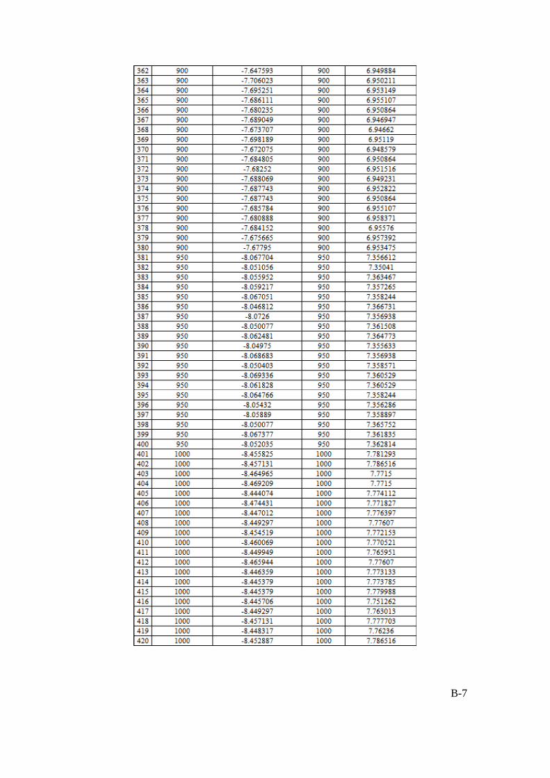
APPENDIX B: CALIBRATION DATA
Table B-1: Load cell calibration raw data.

B-2

B-3

B-4
B-5
B-6
B-7


C-1
APPENDIX C: MATLAB CODE
MATLAB code to get lift force vs. rotating speed for each propeller:
clear all;
rpm = importdata('rpm_296_1.txt'); % raw data in voltage [V]
force = importdata('force_296_1.txt'); % raw data in voltage [V]
M = 113 + 12.7; % total mass (including the motor, the propeller, and
the top fixture of the load cell) [g]
g = 9.81; % gravity [m/s^2]
fs = 20000; % sampling rate
N = 8192; % sample number
D = 0.2032; % diameter of the propeller (0.2032 for 8'', 0.2286 for
9'', 0.254 for 10'') [m]
P = 992.5 * 10^2; % atmospheric pressure [Pa]
T = 18.5 + 273.15; % ambiant temperature [K]
rho = P / T / 287; % air density [kg/m^3]
for (i = 1: 81920);
if force(i) > 0;
force(i) = (68.622865 + 131.406045 * force(i) + M) * g / 1000;
else
force(i) = (32.095052 + 130.208333 * force(i) + M) * g / 1000;
end
end
for (j = 1: 10);
% average force
lift(j, 1) = mean(force(N * (j - 1) + 1: N * j));
lift_std(j, 1) = std(force(N * (j - 1) + 1: N * j));
% fft
C-2
S = rpm(N * (j - 1) + 1: N * j);
Y = fft(S, N);
mag = abs(Y) / (N / 2);
mag(1) = 0;
f = ([1: N] - 1) * fs / N;
for (k = 1: 500)
if mag(k) > 0.5;
break;
end
end
n(j, 1) = (k - 1) * fs / N * 30; % 30 for 2-Blade and 20 for 3-
Blade
% lift coefficient
c_l(j, 1) = lift(j, 1) / rho / (n(j, 1) / 60)^2 / D^4;
end
figure (11);
plot(n, lift, '*r')
axis([0 14000 0 5])
xlabel('\Omega [RPM]')
ylabel('L [N]')
legend('2-9\times6E Trial1')
figure (12);
plot(n, c_l, '*r')
%axis([0 14000 0 0.1])
xlabel('\Omega [RPM]')
ylabel('C_L')
legend('2-9\times6E Trial1')
%dlmwrite('r296_1.txt', n, 'newline','pc');
%dlmwrite('l296_1.txt', lift, 'newline','pc');
%dlmwrite('c296_1.txt', c_l, 'newline','pc');
%dlmwrite('ls296_1.txt', lift_std, 'newline','pc');

C-3
MATLAB code to get repeatability test results:
clear all;
r296_1 = importdata('r296_1.txt');
l296_1 = importdata('l296_1.txt');
c296_1 = importdata('c296_1.txt');
r296_2 = importdata('r296_2.txt');
l296_2 = importdata('l296_2.txt');
c296_2 = importdata('c296_2.txt');
r296_3 = importdata('r296_3.txt');
l296_3 = importdata('l296_3.txt');
c296_3 = importdata('c296_3.txt');
% repetability
figure (1);
plot(r296_1, l296_1, 'rs', r296_2, l296_2, 'b*', r296_3, l296_3,
'k^')
hold on;
plot(r296_1, l296_1, 'r', r296_2, l296_2, 'b', r296_3, l296_3,
'k','LineWidth', 2)
axis([0 14000 0 5])
xlabel('\Omega [RPM]','Fontsize',12)
ylabel('L [N]','Fontsize',12)
legend('Nov 30^{th}','Dec 2^{nd}','Dec 4^{th}',2)
title('2-9\times6E','FontSize',12)
set(gca,'FontSize',12)
%saveas(gcf,'repeat_296_l','png')
figure (2);
plot(r296_1, c296_1, 'rs', r296_2, c296_2, 'b*', r296_3, c296_3,
'k^')
hold on;
plot(r296_1, c296_1, 'r', r296_2, c296_2, 'b', r296_3, c296_3,
'k','LineWidth', 2)
axis([0 14000 0 0.06])
xlabel('\Omega [RPM]','Fontsize',12)
ylabel('C_L','Fontsize',12)
legend('Nov 30^{th}','Dec 2^{nd}','Dec 4^{th}',4)
title('2-9\times6E','FontSize',12)
set(gca,'FontSize',12)
%saveas(gcf,'repeat_296_c','png')

C-4
MATLAB code to get propeller characteristics comparison:
clear all;
r286 = importdata('r286_3.txt');
l286 = importdata('l286_3.txt');
c286 = importdata('c286_3.txt');
r285 = importdata('r285_3.txt');
l285 = importdata('l285_3.txt');
c285 = importdata('c285_3.txt');
r284 = importdata('r284_2.txt');
l284 = importdata('l284_2.txt');
c284 = importdata('c284_2.txt');
r384 = importdata('r384_3.txt');
l384 = importdata('l384_3.txt');
c384 = importdata('c384_3.txt');
r296 = importdata('r296_3.txt');
l296 = importdata('l296_3.txt');
c296 = importdata('c296_3.txt');
r395 = importdata('r395_1.txt');
l395 = importdata('l395_1.txt');
c395 = importdata('c395_1.txt');
r2106 = importdata('r2106_2.txt');
l2106 = importdata('l2106_2.txt');
c2106 = importdata('c2106_2.txt');
% compare effect of pitch
figure (1);
plot(r286, l286, 'rs', r285, l285, 'b*', r284, l284, 'k^')
hold on;
plot(r286, l286, 'r', r285, l285, 'b', r284, l284, 'k','LineWidth',
2)
axis([0 14000 0 5])
xlabel('\Omega [RPM]','Fontsize',12)
ylabel('L [N]','Fontsize',12)
legend('2-8\times6E','2-8\times5E','2-8\times4E',2)
title('Effect of Pitch','FontSize',12)
C-5
set(gca,'FontSize',12)
%saveas(gcf,'pitch_l','png')
figure (2);
plot(r286, c286, 'rs', r284, c284, 'b*', r285, c285, 'k^')
hold on;
plot(r286, c286, 'r', r284, c284, 'b', r285, c285, 'k','LineWidth',
2)
axis([0 14000 0 0.06])
xlabel('\Omega [RPM]','Fontsize',12)
ylabel('C_L','Fontsize',12)
legend('2-8\times6E','2-8\times5E','2-8\times4E',2)
title('Effect of Pitch','FontSize',12)
set(gca,'FontSize',12)
%saveas(gcf,'pitch_c','png')
% compare effect of diameter
figure (3);
plot(r2106, l2106, 'rs', r296, l296, 'b*', r286, l286, 'k^')
hold on;
plot(r2106, l2106, 'r', r296, l296, 'b', r286, l286, 'k','LineWidth',
2)
axis([0 14000 0 7])
xlabel('\Omega [RPM]','Fontsize',12)
ylabel('L [N]','Fontsize',12)
legend('2-10\times6E','2-9\times6E','2-8\times6E',2)
title('Effect of Diameter','FontSize',12)
set(gca,'FontSize',12)
%saveas(gcf,'diameter_l','png')
figure (4);
plot(r286, c286, 'rs', r296, c296, 'b*', r2106, c2106, 'k^')
hold on;
plot(r286, c286, 'r', r296, c296, 'b', r2106, c2106, 'k','LineWidth',
2)
axis([0 14000 0 0.06])
xlabel('\Omega [RPM]','Fontsize',12)
ylabel('C_L','Fontsize',12)
legend('2-10\times6E','2-9\times6E','2-8\times6E',2)
title('Effect of Diameter','FontSize',12)
set(gca,'FontSize',12)
%saveas(gcf,'diameter_c','png')

C-6
% compare effect of number of blades
figure (5);
plot(r395, l395, 'rs', r296, l296, 'b*')
hold on;
plot(r395, l395, 'r', r296, l296, 'b','LineWidth', 2)
axis([0 14000 0 5])
xlabel('\Omega [RPM]','Fontsize',12)
ylabel('L [N]','Fontsize',12)
legend('3-9\times5E','2-9\times6E',2)
title('Effect of Blade Number','FontSize',12)
set(gca,'FontSize',12)
%saveas(gcf,'blade_l','png')
figure (6);
plot(r395, c395, 'rs', r296, c296, 'b*')
hold on;
plot(r395, c395, 'r', r296, c296, 'b','LineWidth', 2)
axis([0 14000 0 0.06])
xlabel('\Omega [RPM]','Fontsize',12)
ylabel('C_L','Fontsize',12)
legend('3-9\times5E','2-9\times6E',2)
title('Effect of Blade Number','FontSize',12)
set(gca,'FontSize',12)
%saveas(gcf,'blade_c','png')
% compare together
figure (7);
plot(r284, l284, 'b*', r286, l286, 'rs', r296, l296, 'mo', r395,
l395, 'k^')
hold on;
plot(r284, l284, 'b', r286, l286, 'r', r296, l296, 'm',r395, l395,
'k', 'LineWidth', 2)
axis([0 13000 0 5])
xlabel('\Omega [RPM]','Fontsize',12)
ylabel('L [N]','Fontsize',12)
legend('2-8\times5E','2-8\times6E', '2-9\times6E','3-9\times5E',2)
title('Effect of Diameter, Pitch, and Blade Number','FontSize',12)
set(gca,'FontSize',12)
saveas(gcf,'together_l','png')
figure (8);
plot(r284, c284, 'b*', r286, c286, 'rs', r296, c296, 'mo', r395,
c395, 'k^')
C-7
hold on;
plot(r284, c284, 'b', r286, c286, 'r', r296, c296, 'm', r395, c395,
'k','LineWidth', 2)
axis([0 13000 0 0.06])
xlabel('\Omega [RPM]','Fontsize',12)
ylabel('C_L','Fontsize',12)
legend('2-8\times5E','2-8\times6E', '2-9\times6E','3-9\times5E',4)
title('Effect of Diameter, Pitch, and Blade Number','FontSize',12)
set(gca,'FontSize',12)
saveas(gcf,'together_c','png')


D-1
APPENDIX D: LABVIEW PROGRAM
Figure D-1: LabVIEW front panel.
Figure D-2: LabVIEW block diagram.

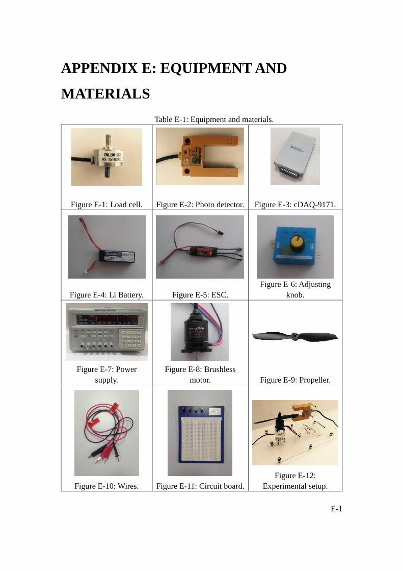
E-1
APPENDIX E: EQUIPMENT AND
MATERIALS
Table E-1: Equipment and materials.
Figure E-1: Load cell.
Figure E-2: Photo detector.
Figure E-3: cDAQ-9171.
Figure E-4: Li Battery.
Figure E-5: ESC.
Figure E-6: Adjusting
knob.
Figure E-7: Power
supply.
Figure E-8: Brushless
motor.
Figure E-9: Propeller.
Figure E-10: Wires.
Figure E-11: Circuit board.
Figure E-12:
Experimental setup.


F-1
APPENDIX F: AUTOCAD DRAWING
Figure F-1: AutoCAD of the base.

F-2
Figure F-2: AutoCAD of the load cell fixture.
Figure F-3: AutoCAD of the wind shield.


