
Measuring the Timing Ability of Fixed Income Mutual Funds
by Yong Chen Wayne Ferson Helen Peters first draft: November 25, 2003 this revision: March 9, 2006 * Ferson and Peters are Professors of Finance at Boston College, 140 Commonwealth Ave, Chestnut Hill, MA. 02467, and Ferson is a Research Associate of the NBER. He may be reached at (617) 552-6431, fax 552-0431, [email protected], www2.bc.edu/~fersonwa. Peters may be reached at (617) 552-3945, [email protected]. Chen is a Ph.D student at Boston College, and may be reached at [email protected]. We are grateful to participants in workshops at Baylor University, Brigham Young, Boston College, DePaul, the University of Florida, Georgetown, the University of Iowa, the University of Massachusetts at Amherst, Michigan State University, the University of Michigan and Virginia Tech. and the Office of Economic Analysis, Securities and Exchange Commission for feedback, as well as to participants at the following conferences: The 2005 Global Finance Conference at Trinity College, Dublin, the 2005 Southern Finance and the 2005 Western Finance Association Meetings. We also appreciate helpful comments from Nadia Voztioblennaia.

ABSTRACT
Measuring the Timing Ability of Fixed Income Mutual Funds
This paper evaluates the ability of US fixed income mutual funds to time common factors related to bond markets. A methodological challenge is to control for potential non-timing-related sources of nonlinearity in the relation between fund returns and common factors. Nonlinearities may arise from dynamic trading strategies or derivatives, funds' responses to public information, they may appear in the underlying assets held by the fund, or they may be related to systematic patterns in stale pricing. Controlling for these effects we find that funds' returns are more typically nonlinear in nine common factors than are fixed-weight benchmark returns. This is an incomplete draft

1. Introduction
The relative share of academic work on bond funds is dwarfed by the share and
importance of these funds and assets in the economy. Elton, Gruber and Blake (1993,
1995) and Ferson, Henry and Kisgen (2006) study US bond mutual fund performance,
concentrating on the funds' risk-adjusted returns, or alphas. These studies find that the
typical average performance after costs is negative and on the same order of magnitude as
the funds' expenses. However, the total performance may be decomposed into
components, such as timing and selectivity ability. If investors place value on timing
ability, for example a fund that can mitigate losses in down markets, they may accept a
total performance cost for this service. To better understand performance we need to
examine its components. We argue that a logical place to start, in the case of fixed income
funds, is to study timing ability.1 That is the goal of this paper. This is one of the first
papers to comprehensively study the ability of US bond funds to time their markets.2
Timing ability on the part of a fund manager is the ability to use information about
the future realizations of common factors affecting security returns. Selectivity refers to
the use of security-specific information. If common market factors explain a relatively
large part of the variance of a typical bond return, it follows that a relatively large fraction
of the potential performance of bond funds is likely attributed to timing. Thus, a logical
step in looking at performance is to concentrate on timing ability. However, measuring
1 We do not explicitly study market timing in the sense recently taken to mean trading by investors in a fund to exploit stale prices reflected in the fund's net asset values, or late trading -- potentially fraudulent trading after the close of the market. But we will see that these issues can affect measures of a fund manager's ability.
2 Brown and Marshall (2001) develop an active style model and an attribution model for fixed income funds, isolating managers' bets on interest rates and spreads. Comer, Boney and Kelly (2005) study timing ability in a sample of 84 high quality corporate bond funds, 1994-2003, using variations on Sharpe's (1992) style model. Comer (2006) measures bond fund sector timing using portfolio weights. Aragon (2005) studies the timing ability of balanced funds for bond and stock indexes.

2
the timing ability of fixed income funds is a subtle problem.
Traditional models of market timing ability rely on convexity in the relation
between the fund's returns and the common factors.3 In bond funds, perhaps even more
clearly than in equity funds, convexity or concavity can arise for various reasons unrelated
to timing ability. Our empirical analysis controls for other sources of nonlinearity. These
include convexity or concavity that may be inherent in the benchmark assets held by a
fund, the use of dynamic trading strategies or derivatives, portfolios that respond to
publicly available information and stale prices in the measured returns.
Most versions of the models with the controls for non-timing-related nonlinearities
find that funds' returns are more typically nonlinearly related to nine common factors
than are fixed-weight benchmark returns. We find evidence of positive timing ability for
some factors, including credit spreads and the relative value of the dollar. There is also
evidence of "negative" timing ability for some factors, including interest rates, mortgage
spreads and bond market liquidity. Negative timing is similar to what previous studies
have found for equity funds relative to the stock market. However, unlike the case of
equity funds, conditional models (e.g. Ferson and Schadt, 1996) do not explain the
nonlinearity.
The rest of the paper is organized as follows. Section 2 describes the models and
methods. Section 3 describes the data. We study timing relative to a set of seven bond
market factors and two equity market factors. Section 4 presents our empirical results and
Section 5 offers some concluding remarks.
3 The alternative approach is to examine managers' portfolio weights and trading decisions to see if they can predict returns and factors (e.g. Grinblatt and Titman, 1989). Comer (2006) is a first step in this direction for bond funds.

3
2. Models and Methods
A traditional view of performance separates timing ability from security selection ability,
or selectivity. For equity funds, timing is closely related to asset allocation, where funds
rebalance the portfolio among asset classes and cash. Selectivity essentially means picking
good stocks within the asset classes. Like equity funds, fixed income funds engage in
activities that may be viewed as selectivity or timing.
Fixed income funds may attempt to predict institution-specific supply and demand
or changes in credit risks associated with particular bond issues. Funds can also attempt
to exploit liquidity differences across bonds, for example on-the-run versus off-the-run
issues. These trading activities are akin to security selection. In addition, managers may
tune the interest rate sensitivity (e.g., duration) of the portfolio to time changes in the level
of interest rates or the shape of the yield curve in anticipation of the influence of economic
developments. They may vary the allocation to asset classes (e.g. corporates versus
governments versus mortgages) that are likely to have different exposures to economic
factors. These activities may naturally be considered as attempts at "market timing," since
they relate to anticipating market-wide factors.
Classical models of market-timing ability consider an equity manager who chooses
a portfolio consisting of a market index and Treasury bills. The manager observes a signal
about the future relative performance of the market over bills, and adjusts the market
exposure of the portfolio. If the response is assumed to be a linear function of the signal as
modelled by Admati, Ross and Plfeiderer (1986), the portfolio return is a convex quadratic
function of the market return as in the model of Treynor and Mazuy (1966). If the
manager shifts the portfolio weights discretely, as in the model of Merton and Henriksson
(1981), the resulting convexity may be modelled with call options. Jiang (2003) develops a
timing measure based on the probability, but not the magnitude of a convex relation. In

4
each case the convexity in the relation between the fund return and the market return
indicates the timing ability. Our models modify this classical set up to accommodate
nonlinearities unrelated to managers' timing ability.
2.1 Classical Market Timing Models
The classical market-timing regression of Treynor and Mazuy (1966) is:
rpt+1 = ap + bp ft+1 + Λp ft+12 + ut+1, (1)
where rpt+1 is the fund's portfolio return, measured in excess of a short-term Treasury bill.
With equity market timing, as considered by Treynor and Mazuy, ft+1 is the excess return
of the stock market index. Treynor and Mazuy (1966) argue that Λp>0 indicates market-
timing ability. The logic is that when the market is up, the successful market-timing fund
will be up by a disproportionate amount. When the market is down, the fund will be
down by a lesser amount. Therefore, the fund's return bears a convex relation to the
market factor.
In a fixed income context it seems natural to replace the market excess return with
systematic factors for bond returns. However, if a factor is not an excess return, the
appropriate sign for the coefficient might not be obvious. For example, bond returns
move in the opposite direction as interest rates, so a signal that interest rates are about to
rise means bond returns are likely to be low. We show below that market timing ability
still implies a positive coefficient on the squared factor.
Stylized market-timing models confine the fund to a single risky-asset portfolio and
cash. This makes sense theoretically, from the perspective of the Capital Asset Pricing
Model (CAPM, Sharpe, 1964). Under that model's assumptions there is two-fund

5
separation and all investors hold the market portfolio and cash. But two-fund separation
is generally limited to single-factor term structure models, and there is no central role for a
"market portfolio" of bonds in most fixed income models. In practice, however, fixed
income funds often manage to a "benchmark" portfolio that defines the peer group or
investment style. We use style-specific benchmarks to replace the market portfolio.
Assume that the fund manager combines a benchmark portfolio with return RB and
a short-term Treasury security or "cash" with known return Rf, using the portfolio weight
x(s), where s is the private timing signal. The managed portfolio return is Rp = x(s)RB + [1-
x(s)]Rf. The signal is observed and the weight is set at time t, the returns are realized at
time t+1, and we suppress the time subscripts for simplicity. In the simplest example the
factor and the benchmark's excess return are related by a linear regression (we allow for
nonlinearities below):
rBt+1 = μB + bB ft+1 + uBt+1, (2)
where rB = RB - RF is the excess return, μB=E(rB), the factor is normalized to have a mean
of zero and uBt+1 is independent of ft+1. Assume that the signal s = f + v, where v is an
independent, mean zero noise term with variance, σv2. The manager is assumed to
maximize the expected value of an increasing, concave expected utility function,
E{U(rp)|s}. Finally, assume that the random variables (r,f,s) are jointly normal and let σf2 =
Var(f). With these assumptions the optimal portfolio weight of the market timer is:4
4 The first order condition for the maximization implies: E{U'(.)rB|s} = 0 = E{U'(.)|s} E{rB|s} + Cov(U'(.),rB|s}, where U'(.) is the derivative of the utility function. Using Stein's (1973) lemma, write the conditional covariance as: Cov(U'(.),rB|s} = E{U''(.)|s} x(s) Var(rB|s). Solving for x(s) gives the result, with λ = -E{U'(.)|s}/E{U''(.)|s} > 0.

6
x(s) = λ E(rB|s)/σB2, (3)
where λ > 0 is the Rubinstein (1976) measure of risk tolerance, which is assumed to be a
fixed parameter, and σB2 = Var(rB|s), which is a fixed parameter under normality.
The implied regression for the managed portfolio's excess return follows from the
optimal timing weight x(s) and the regression (2). We have rp = x(s) rB, then substituting
from (2) and (3) and using E(rB|s) = μB + bB [σf2/(σf2 + σv2)] (f+v), we obtain equation (1),
where ap = λμB2/σB2, bp = (λμBbB/σB2) [1 + σf2/(σf2+σv2)] and Λp = (λ/σB2)bB2
[σf2/(σf2+σv2)]. The error term upt+1 in the regression is a linear function of uB, v, vuB, fuB
and vf. The assumptions of the model imply that the regression error is well specified,
with E(up f) = 0 = E(up) = E(up f2).
The simple model illustrates that timing ability implies convexity between the
fund's return and a systematic factor that is linearly related to the benchmark return. Note
that if λ>0 the coefficient Λp ≥ 0, independent of the sign of bB. Also, if the manager does
not receive an informative signal, then Λp=0, as E(rB|s) and x(s) are constants in that case.
However, the simple model does not consider nonlinearity in the fund's return that may
arise for reasons unrelated to timing ability. In order to obtain reliable measures of timing
ability, it is necessary to extend the model to control for these other potential sources of
nonlinearity.
2.2 Nonlinearity Unrelated to Timing
Convexity or concavity is likely to arise when the underlying assets held by a fund
bear a nonlinear relation to the common factors. While this may occur in equity funds,
such nonlinearities are likely in bond funds. Even simple bond returns are nonlinearly

7
related to interest rate changes, and securities such as mortgage products are described in
terms of their "negative convexity" with respect to interest rate factors.
A second potential cause of nonlinearities is "interim trading," as described by
Goetzmann, Ingersoll and Ivkovic (2000), Ferson and Khang (2002) and Ferson, Henry and
Kisgen (2006). This refers to a situation where fund managers trade more frequently than
the fund's returns are measured. With monthly fund return data, interim trading
definitely occurs. Derivatives may often be replicated by dynamic trading, so the use of
derivatives is a closely related issue. For example, a fund that holds call options bears a
convex relation to the underlying asset, and that can be confused with market timing
ability (Jagannathan and Korajczyk, 1986).5
A third reason for nonlinearity, unrelated to timing ability, arises if there is public
information about future asset returns, and if managers' portfolios respond to this public
information. As shown by Ferson and Schadt (1996), even if the conditional relation is
linear, the response to public information can induce nonlinearities in the unconditional
relation between the fund and a benchmark return. In this case the portfolio weights at
the beginning of the period are correlated with returns over the subsequent period, due to
their common dependence on the public information, and the products of the weights and
the returns are nonlinear. Nonlinearity from public information trading can occur even if
there is no interim trading problem.
The fourth potential reason for nonlinearity unrelated to timing ability is stale
pricing of a fund's underlying assets. Thin or nonsynchronous trading in a portfolio has
5 In another example, Brown et al. (2004) explore arguments that incentives and behavioral biases can induce managers to engage in option-like trading within performance measurement periods, even if they have no superior information. The fund's investors are "short" any option-like compensation provided to fund managers, and the fund's measured return, which is net of manager compensation, could bear a nonlinear relation to the benchmark.

8
long been known to bias beta estimates for the portfolio (e.g., Scholes and Williams, 1977).
We show that if the degree of nonsynchronous trading is related to a common factor, this
"systematic" stale pricing can create additional spurious concavity or convexity. The
following subsections describe our approaches to controlling for these issues.
2.3 Addressing Nonlinearity in Benchmark Assets
We generalize the classical market timing model to handle nonlinearity in the
relation between the benchmark asset returns and the common factors. To do this we
replace the linear regression (2) with a nonlinear regression:
rBt+1 = aB + bB(ft+1) + uBt+1, (4)
where bB(f) is a nonlinear function, specified below, and we assume that uB and bB(f) are
normal and independent. The manager's market-timing signal is now assumed to be s =
bB(f) + v, where v is normal independent noise with variance, σv2. This captures the idea
that the manager focusses on the return implications of information about the common
factor.
With these modifications the optimal weight function in (3) obtains with:
E(rB|s) = μB [σv2/(σf*2 + σv2)] + [σf*2/(σf*2 + σv2)][aB + bB(f) + v], where σf*2=Var(bB(f)).
Substituting as before we derive the nonlinear regression for the portfolio return:
rpt+1 = ap + bp [bB(ft+1)] + Λp [bB(ft+1)]2 + ut+1, (5)
with: ap = λ aB(μB σv2 + aB σf*2)/[σB2(σf*2+σv2)],
bp = λ(μB σv2 + 2aB σf*2)/[σB2(σf*2+σv2)],
and Λp = (λ/σB2)[σf*2/(σf*2+σv2)].

9
The model restricts the coefficients in the nonlinear regression of the fund's return on the
factors. The intuition is that nonlinearity of the benchmark return partly determines the
nonlinearity of the fund's return. If there is no market-timing signal, then x(s) is a
constant, Λp=0 in (5) and the nonlinearity of the fund's return mirrors that of the
benchmark. A successful market timer has a convex relation, relative to the benchmark,
and thus Λp>0. For example, if the benchmark is convex in the factor, a market-timing
fund is more convex than the benchmark. We combine equations (4) and (5), and estimate
the model by the Generalized Method of Moments (Hansen, 1982).
One of the forms for bB(f) that we examine is a quadratic function. This has an
interesting interpretation in terms of systematic co-skewness. Asset-pricing models
featuring systematic coskewness with a market factor are studied, for example, by Kraus
and Litzenberger (1976). Equation (1) is, in fact, equivalent to the quadratic "characteristic
line" used by Kraus and Litzenberger, when the factor is the market portfolio excess
return. The coefficient on the squared market factor measures the systematic coskewness
risk of the portfolio, and this may have nothing to do with market timing. Thus, a fund's
return can bear a convex relation to the factor because it holds assets with positive
coskewness risk. Equation (5) allows the benchmark to have coskewness risk when bB(f)
is quadratic. When Λp=0 and the manager has no timing ability, the fund inherits its
coskewness from the benchmark. If the fund has timing ability, Λp>0 measures the
additional convexity generated by the timing ability.
2.4 Addressing Interim Trading
Interim trading means that fund managers trade more frequently than the fund's
returns are measured. This can lead to spurious inferences about market timing ability, as

10
shown by Goetzmann, Ingersoll and Ivkovic (2000) and Jiang, Yao and Yu (2005), and can
also lead to incorrect inferences about total performance, as shown by Ferson and Khang
(2002). Ferson, Henry and Kisgen (2006) propose a solution, starting with a continuous-
time asset pricing model. The continuous-time model prices all portfolio strategies that
may trade within the period, provided that the portfolio weights are nonanticipating
functions of the state variables in the model. If the continuous-time model can price
derivatives by replication with dynamic strategies, the use of derivatives is also covered
by this approach.
Ferson, Henry and Kisgen derive the stochastic discount factor (SDF) for a set of
popular term structure models, that applies to discrete-period returns and allows for
interim trading during the period from time t to time t+16:
tmt+1 = exp(a - Art+1 + b'Axt+1 + c'[xt+1 - xt]), (6)
where x is the vector of state variables in the model. The terms Axt+1 = Σi=1,...1/Δ x(t+(i-1)Δ)Δ
approximate the integrated levels of the state variables. The measurement period
between t and t+1 is one month, matching observed fund returns, and the period is
divided into pieces of length Δ=one trading day. Art+1 is the similarly time-averaged level
of the short-term interest rate. The empirical "factors," ft+1, in the SDF thus include the
discrete monthly changes in the state variables, their time averages and the time-averaged
short term interest rate: ft+1 = {[xt+1-xt], Axt+1, Art+1}.
With the approximation ef ≈ 1+f, we can consider a model in which the SDF is
linear in the expanded set of empirical factors. Using a linear function for the SDF is
6 A stochastic discount factor is a random variable, tmt+1, that "prices" assets through the equation Et{tmt+1 Rt+1}=1.

11
equivalent to using a beta pricing model for expected returns, written in terms of the
relevant factors (Dybvig and Ingersoll (1982), Ferson, 1995). This motivates including the
time-averaged variables in regressions like (5), as additional factors to control for interim
trading effects.7
2.5 Addressing Public Information
A nonlinear relation between a fund's return and common factors may arise if
managers respond to public information and there is time variation in factor risk
premiums. Such time variation may be even more likely for bond returns than for stock
returns. Conditional timing models have been designed to control for these effects by
allowing portfolio weights and funds' betas to vary over time with public information.
Using equity funds, Ferson and Schadt (1996) and Becker, et al. (1999) find that such
conditional timing models are better specified than models that do not control for public
information. In particular, Ferson and Schadt (1996) propose a conditional version of the
market timing model of Treynor and Mazuy (1966):8
rpt+1 = ap + bp rBt+1 + Cp'(Zt rBt+1) + Λp rBt+12 + ut+1. (7)
7 Equation (6) also motivates the use of an exponential function for bB(f) in Equation (4). Under an exponential function the squared term in a market timing model like (5) is perfectly correlated with the linear term, so we don't estimate this case separately. An exponential function for bB(f) is closely approximated by a linear function when the factor changes are small numbers.
8 Ferson and Schadt (1996) also derive a conditional version of the market timing model of Merton and Henriksson (1981), which views successful market timing as analogous to producing cheap call options. This model is considerably more complex than the conditional Treynor-Mazuy model, and they find that it produces similar results.

12
In Equation (7), the new term Cp'(Zt rBt+1) controls for nonlinearity due to the
public information, Zt. The expected benchmark return and the manager's optimal
portfolio weights both depend on Zt. This induces common time-variation in the
benchmark return and the fund's "beta" on the benchmark. The term C'(ZtrBt+1) captures
this common variation, controlling for the "spurious" timing effect due to public
information.
In a regression like (7) we measure timing with respect to the benchmark return, rB.
However, we are also interested in timing with respect to interest rates and other
economic factors that may bear a nonlinear relation to the benchmark, as described above.
We study timing ability for these factors by replacing rB in Equation (7) with the nonlinear
function bB(f) and estimating the equations (4) and (7) together in a system.
2.6 Addressing Stale Prices
Thin or nonsynchronous trading in a portfolio biases estimates of the portfolio beta
(e.g., Scholes and Williams, 1977). A similar effect occurs when the measured value of a
fund reflects stale prices (e.g. Getmansky, Lo and Makarov, 2004). If the extent of stale
pricing is related to a common factor, we call it "systematic" stale pricing. Systematic stale
pricing can create spurious concavity or convexity and thus a spurious impression of
market timing ability.
To address the stale pricing issue we use a simple model in the spirit of Getmansky,
Lo and Makarov. Let pt be the natural log of the fund's "true" net asset value per share
with the last period's dividends reinvested, so that rt = pt - pt-1 is the true return. The true
return would be the observed return if no prices were stale. We assume rt is independent
over time with mean μ. The measured price, pt* is given by δt pt-1 + (1-δt) pt, where the
coefficient δt ε [0,1] measures the extent of stale pricing during the month t. The

13
measured return on a fund, rt*, is then given by:
rt* = δt-1rt-1 + (1-δt)rt, (8)
Assume that the market or factor return rmt, with mean μm and variance σm2, is iid over
time and measured without error.9
To model stale pricing that may be systematic, consider a regression of the extent of
stale pricing at time t on the market factor:
δt = δ0 + δ1(rmt - μm) + εt, (9)
where we assume that εt is independent of the other variables in the model. We are
interested in moments of the true return, like Cov(rt,rmt2), which measures the timing
ability. Straightforward calculations relate the moments of the observable variables to the
moments of the unobserved variables, as follows.
E(r*) = μ (10a)
Cov(rt*,rmt) = Cov(r,rm)(1- δ0 + 2δ1μm) - δ1 {μ σm2 + Cov(r,rm2)} (10b)
Cov(rt*,rmt2)= Cov(r,rm2)(1- δ0 + δ1μm) - δ1{ μE(rm3) + Cov(r,rm3) - [Cov(r,rm)+μμm](μm2+σm2)} (10c)
Cov(rt*,rmt) + Cov(rt*,rmt-1) = Cov(r,rm) (10d)
Cov(rt*,rmt2) + Cov(rt*,rmt-12) = Cov(r,rm2) (10e)
Cov(rt*,rmt3) + Cov(rt*,rmt-13) = Cov(r,rm3) (10f)
9 We have considered models in which the benchmark return rm also has stale pricing, and find that the number of parameters proliferates to the point of intractability. Thus, our estimates of this model should in practice capture fund staleness relative to any staleness in the benchmark return.

14
Equation (10a) shows that stale prices will not affect the measured average returns
in this model, even if stale pricing is systematic.10 Equation (10b) captures the bias in the
measured covariance with the market. The market beta, of course, is this covariance
divided by the market variance. If δ1=0 stale pricing is not systematic, and the effect on
the measured beta reduces to an attenuation bias as in the model of Scholes and Williams
(1977). If δ1 is not zero stale pricing is systematic, and the measured beta is affected by
both stale pricing and the true timing ability. Equation (10c) shows that the measured
timing coefficient is also biased. If the stale pricing is not systematic, however, the bias
reduces to a scale factor. If δ1=0 we can therefore test the null hypothesis of no timing
ability using the measured covariance, as the true timing coefficient is zero if and only if
the measured covariance with the squared market factor is zero (assuming that δ0≠1).
When stale pricing is systematic the bias of the timing coefficient is complex as it depends
on the true beta, the value of δ1, higher moments and other parameters. We need to
control for this complicated bias in order to measure the timing ability.
Fortunately, equation (10e) reveals a simple way to control for a biased market
timing coefficient due to stale prices. The sum of the covariances of the measured return
with the squared market factor and the lagged squared factor equals the true covariance
or timing coefficient. This is similar to the bias correction for betas in the models of
Scholes and Williams (1977) and Dimson (1979).
If we append moment conditions to the system (10) to identify μm, σm2 and E(rm3)
we have a system of nine equations that allow us to identify the nine parameters, {μm, σm2,
10 Qian (2005) studies the effects of stale prices on the measured average performance of equity style funds, and finds that if staleness is correlated with new money flows there can be effects on average returns. See Zietowitz (2003) and Edelin (1999) for estimates of the size of potential losses to buy-and-hold investors, attributed to other investors trading on stale net asset values.

15
Cov(r,rm), Cov(r,rm2), E(rm3), Cov(r,rm3), δ0, δ1, and μ}. We estimate the system by the
generalized method of moments (GMM, Hansen, 1982). We measure the timing ability,
adjusted for the effects of stale pricing, via the parameter Cov(r,rm2).
2.7 Combining the Effects
We have models for four different sources of convexity or concavity unrelated to
timing ability, and we may wish to control for all of these effects. The models for interim
trading and public information suggest control variables that may be included in the
market timing regressions, while the nonlinear-benchmark models imply a system of
equations. The general form of the models is a system including Equation (4) and
Equation (11):
rpt = a + β'Xt + Λp [bB(ft)2] + upt, (11)
where Xt is a vector of control variables observed at t or before, and which includes bB(ft),
the benchmark's nonlinear projection on the factor. In the presence of stale pricing we
observe rpt* and not the true return, rpt. However, according to Equation (10e) we can still
estimate the timing coefficient easily if we do not require estimates of the deeper
structural parameters of the model. Simply replacing bB(ft)2 in (11) with the sum, bB(ft)2 +
bB(ft-1)2, delivers a coefficient that should be proportional to Λp.
3. The Data
We first describe our sample of bond funds. We then describe the interest rate and other
economic data that we use to construct the common factors relative to which we study

16
timing ability. Finally, we describe the fund style-related benchmark returns.
3.1 Bond Funds
The fund data are from the Center for Research in Security Prices (CRSP) mutual
fund data base, and include returns for the period from January of 1962 through
December of 2002. We select open-end funds whose stated objectives indicate that they
are bond funds.11 We exclude money market funds and municipal securities funds.
There are a total of 23,281 fund-year records in our initial sample. In order to
address back-fill bias we remove the first year of returns for new funds, and any returns
prior to the year of fund organization, a total of 1345 records. Data may be reported prior
to the year of fund organization, for example, if a fund is incubated before it is made
publicly available (see Elton, Gruber and Blake (2001) and Evans, 2004). Extremely small
funds are more likely to be subject to back-fill bias. We delete cases where the reported
total net assets of the fund is less than $5 million. This removes 3205 records. We delete
all cases where the reported equity holdings at the end of the previous year exceeds 10%.
This removes another 644 records. After these screens we are left with 18,087 fund-years.
The number of funds with some monthly return data in a given year is five at the
beginning of 1962, rises to 17 at the end of 1973, to 617 by 1993 and to 1756 at the end of
11 Prior to 1990 we consider funds whose POLICY code is B&P, Bonds, Flex, GS or I-S or whose OBJ codes are I, I-S, I-G-S, I-S-G, S, S-G-I or S-I. We screen out funds during this period that have holdings in bonds plus cash less than 70% at the end of the previous year. In 1990 and 1991 only the three digit OBJ codes are available. We take funds whose OBJ is CBD, CHY, GOV, MTG or IFL. If the OBJ code is other than GOV, we delete those funds with holdings in bonds plus cash totalling less than 70%. After 1991 we select funds whose OBJ is CBD, CHY, GOV, MTG, or IFL or whose ICDI_OBJ is BQ, BY, GM or GS, or whose SI_OBJ is BGG, BGN, BGS, CGN, CHQ, CHY, CIM, CMQ, CPR, CSI, CSM, GBS, GGN, GIM, GMA, GMB, GSM or IMX. From this group we delete 116 fund years for which the POLICY code is IG or CS.

17
the sample in December of 2002.
We group the funds into equally-weighted portfolios according to fund style. We
define seven styles on the basis of the various objective codes on the CRSP database. The
styles are Global, Short-term, Government, Mortgage, Corporate, High Yield and Other.12
Summary statistics for the style-grouped funds are reported in Panel A of Table 1. The
mean returns are all between 0.31 and 0.56% per month. The standard deviations of
return range between 0.47% per month, for Short-term Bond funds, to 1.66% per month
for High-yield funds. The first-order autocorrelations of the returns range from 8%, for
Global Bond funds, to 30% for High Yield funds. The minimum return across all of the
style groups in any month is -6.7%, suffered in October of 1979 by the corporate bond
funds. The maximum return is 10.3%, also earned by the Corporate bond funds in
November of 1981.
Table 1 also reports the second order autocorrelations of the fund returns. The
stylized thin trading model assumes that thin trading is resolved (all the assets trade)
within two months. This implies that the measured returns have an MA(1) time-series
structure, and the second order autocorrelations should be zero. The largest second order
autocorrelation in the panel is 7.1%, with an approximate standard error of 1/√T = 1/√144
= 8.3%. For the portfolio of all funds, where the number of observations is the greatest,
the second order autocorrelation is -2.2%, with an approximate standard error of 1/√492 =
4.5%. Thus, none of the second order autocorrelations is significantly different from zero,
12 Global funds are coded SI_OBJ=BGG or BGN. Short-term funds are coded SI_OBJ=CSM, CPR, BGS, GMA, GMS or GBS. Government funds are coded OBJ=GS POLICY=GOV, ICDI_OBJ=GS or GB, or SI_OBJ=GIM or GGN. Mortgage funds are coded ICDI_OBJ=GM, OBJ=MTG or SI_OBJ=GMB. Corporate funds are coded as OBJ=CBD, ICDI_OBJ=BQ, POLICY=B&P or SI_OBJ=CHQ, CIM, CGN or CMQ. High Yield funds are coded as ICDI_OBJ=BY, SI_OBJ=CHY or OBJ=CHY or OBJ=I-G and Policy=Bonds. Other funds are defined as funds that we classify as bond funds (see the previous footnote), but which meet none of the above criteria.

18
consistent with the assumptions of the model.
We also group the funds into equally-weighted portfolios according to various
fund characteristics, measured at the end of the previous year. Since the characteristics
are likely to be associated with fund style, we form groups within each of the style
classifications. The characteristics include fund age, total net assets, percentage cash
holdings, percentage of holdings in options, reported income yield, turnover, load
charges, expense ratios, the average maturity of the funds' holdings, and the lagged return
for the previous year. The Appendix provides the details.
3.2 Common Factor Data
We use daily and weekly data to construct monthly empirical factors, including the
discrete changes measured from the ends of the months and the time-averaged values
used as controls for interim trading bias. Most of the data are from the Federal Reserve
(FRED) and the Center for Research in Security Prices (CRSP) databases. The daily
interest rates are from the H.15 release. The factors reflect the term structure of interest
rates, credit and liquidity spreads, exchange rates, a mortgage spread and two equity
market factors.
Three factors represent the term structure of Treasury yields: A short-term interest
rate, a measure of the term slope and a measure of the curvature of the yield curve.
Studies such as Litterman, Sheinkman and Weiss (1991) find that three factors explain
most of the variance of Treasury bond returns across the maturity spectrum, and that
level, slope and curvature provide a convenient way to represent three factors.
The short-term interest rate is the three-month Treasury rate, converted from the
bank discount quote to a continuously compounded yield. Chapman, Pearson and Long
(2001) argue that the three month Treasury rate is a good empirical proxy for the

19
theoretical short-term interest rate. The slope of the term structure is the ten-year yield
less the one-year yield. The curvature measure is the concavity: y3 - (y7 + 2y1)/3, where yj
is the j-year fixed-maturity yield.
Since some of our funds hold corporate bonds subject to default risk and mortgage
backed securities subject to prepayment risks, we construct associated factors. Our credit
spread series is the yield of Baa corporate bonds minus Aaa bonds, from the FRED. This
series is measured as the weekly averages of daily yields. We use the averages of the
weeks in the month for our time-averaged version of the spread. For the discrete changes
in the spread we use the first differences of the last weekly values for the adjacent months.
The first difference series may not be as clean as with daily data, but we are limited by the
data available to us. Our mortgage spread is the difference between the average contract
rate on new conventional mortgages, also available weekly from the FRED, and the yield
on a three-year, fixed maturity Treasury bond. Here we use daily data on the Treasury
bond and weekly data on the mortgage yield to construct the time averages and discrete
changes.
Liquidity is likely to be a relevant factor for bond funds. Liquidity varies both
across issues and over time. For example, on-the-run Treasury issues are more liquid than
off-the-run issues. Also, credit markets have periodic episodes where liquidity gets tight
or loose. For market timing we are interested in market-wide fluctuations in liquidity.
Our measure follows Gatev and Strahan (2005), who advocate a spread of commercial
paper over Treasury yields as a measure of short term liquidity in the corporate credit
markets. We use the yield difference between three-month nonfinancial corporate
commercial paper rates and the three month Treasury yield. The commercial paper rates
are measured weekly, as the averages over business days, and we convert them from the
bank discount basis to continuously compounded yields.

20
Some of the funds in our sample are global bond funds, so we include a factor for
currency risks. Our measure is the value of the US dollar, relative to a trade-weighted
average of major trading partners, from the FRED. This index is measured weekly, as the
averages of daily figures, and we treat it the same way we treat the credit spread data.
Corporate bond funds, and high-yield funds in particular, may be exposed to
equity-related factors. We therefore include two equity market factors in our analysis. We
measure equity volatility with the VIX-OEX index implied volatility. This series is
available starting in January of 1986. We also include an equity market valuation factor,
measured as the log dividend ratio for the CRSP value-weighted index. The dividends are
the sum of the dividends over the past twelve months, and the value is the cum-dividend
value of the index. The level of this ratio is a state variable for valuation levels in the
equity market, and its monthly first difference is used as a factor. The first difference of
this series approximates the (negative of the) continuously-compounded capital gains
component of the index return.
Table 2 presents summary statistics for the monthly common factor series starting
in February of 1962 or later, depending on data availability, and ending in December 2002.
Missing values are excluded and the units are percent per year (except for the dollar
index). Panel A presents the levels of the variables, panel B the monthly first differences
and Panel C presents the time-averaged values.
The average term structure slope was positive, at just under 80 basis points during
the sample period. The average credit spread was about one percent, but varied between
32 basis points to more than 2.8%. The average mortgage spread over Treasuries was just
over 2% for the period starting in 1971, and varied between about -1% to more than 7%.
The liquidity spread averaged 4.7%, with a range between 1.3% and 6.8% over the 1997-
2002 period.
21
In their levels the factors are highly persistent time series, as indicated by the first
order autocorrelation coefficients. Six of the nine are in excess of 90%. The time averaged
factors are also highly persistent, with autocorrelations greater than 84%. Moving to first
differences, the series look more like innovations.13
3.3 Style Index Returns
We construct style-specific benchmarks for the funds from a set of asset-class
returns, using a methodology similar to Sharpe (1992). The problem is to combine the
asset class returns, Ri, using a set of portfolio weights, {wi}, so as to minimize the "tracking
error" between the return of the fund (or fund style group), Rp, and the style-matched
benchmark portfolio, ΣiwiRi. The portfolio weights are required to sum to 1.0 and must be
non-negative, which rules out short positions:
Min{wi} Var[Rp - Σi wiRi], (13)
subject to: Σi wi = 1, wi ≥ 0 for all i,
where Var[.] denotes the variance. We solve the problem numerically, deriving a set of
weights for each fund style group. The asset class returns include US Treasury bonds of
three maturity ranges from CRSP (less than 12 months, less than 48 months and greater
than 120 months), the Lehman Composite Global bond index, the Lehman US Aggregate
13 Given the relatively high persistence and the fact that some of the factors have been studied before exposes us to the risk of spurious regression compounded with data mining, as studied by Ferson, Sarkissian and Simin (2003). However, Ferson, Sarkissian and Simin (2005) find that biases from these effects are largely confined to the coefficients on the persistent regressors, while the coefficients on variables with low persistence are well behaved. Thus, the slopes on our persistent control variables and thus the intercepts may be biased, but the timing coefficients should be well behaved.

22
Mortgage Backed Securities index, the Merrill Lynch High Yield US Master index and the
Lehman Aaa Corporate bond index.14
Panel B of Table 1 presents the style-index weights for each of the style portfolios.
The weights reported in the table do not sum exactly to 1.0 due to rounding errors, but we
carry many more digits of precision in the return calculations. The weights present
sensible patterns in most cases, suggesting that both the style classification of the funds
and Sharpe's procedure are reasonably valid. The global funds load most heavily on
corporate bonds and global bonds, then on low quality bonds. Short term funds have
most of their weight in bonds with less than 48 months to maturity. Mortgage funds have
their greatest weights on mortgage backed securities and shorter term bonds. Corporate
funds have more than 50% of their weight in high or low grade corporate bonds. High
yield funds have 70% of their weight in low grade corporate bonds. Government funds
load highly on mortgage-backed securities (33%). This is consistent with the portfolio
weights described by Comer (2006), who finds that government style bond funds allocate
about 1/3 of their portfolios to mortgage related securities.
4. Empirical Results
We first examine the empirical relations between the various factors, the fund groups and
passive investment strategies proxied by the Sharpe style benchmarks. We estimate the
model of stale pricing and evaluate the effects of the other controls for nonlinearities
unrelated to timing. Finally, we apply the adjusted timing measures to individual funds.
14 We splice the Blume, Keim and Patel (1991) low grade bond index prior to 1991, with the Lehman High Yield index after that date. We splice the Ibbotson Associates 20 year government bond return series for 1962-1971, with the CRSP greater than 120 month government bond return after 1971.

23
4.1 Factor Models
We begin the empirical analysis with regressions of the Sharpe style benchmark
returns on changes and squared changes in the common factors, looking for convexity or
concavity in these relations. Any nonlinearity would appear in a naive application of the
timing regression (1) for funds, if funds simply held the benchmarks. These regressions
are shown in Panel A of Table 3. Panel B of Table 3 shows regressions for the mutual
funds' returns, grouped by the same style categories. Comparing the funds with the style
benchmarks provides a feel for the affects of active management. The table shows the
coefficients on the squared terms for the regressions, run one factor at a time.
The coefficients for the style benchmarks in Panel A of Table 3 present some
interesting patterns. Out of 63 cases (seven styles x 9 factors) there are only five
heteroskedasticity-consistent t-ratios on the squared factors with absolute values larger
than two. However, 21 of the absolute t-ratios are between 1.6 and 2.0, which provides
some evidence of nonlinearity. Most of the coefficients on the squared factors are positive
-- only eight of the 63 are less than zero. This means that we would expect to measure
weak convexity or timing ability, based on regression (1), if funds simply held the
benchmarks.
The coefficients for the mutual funds in Panel B of Table 3 tell a different story. We
find 13 absolute t-ratios larger than 2.0. This is more than expected by chance; thus, the
mutual fund returns are significantly nonlinearity related to the factors.15 Furthermore,
the coefficients on the squared factors are negative in about half the cases; whereas, most
15 Using a simple binomial model assuming independence, the t-ratio associated with finding 13 "rejections," when the probability of observing a rejection is 5%, is (13/63 - .05)/(.05(.95)/63)0.5 = 5.69.

24
of the coefficients were positive for the benchmarks. Thus, overall the fund returns
appear more concave in relation to the factors than the benchmark returns. This suggests
poor market timing ability on the part of the mutual funds. Alternatively, the concavity
could reflect derivatives or dynamic trading, public information or stale prices.
The right-hand column of Table 3 presents the R-squares of the factor model
regressions, using all of the factors simultaneously. The fractions of the fund return
variances explained by the factors are interesting because large fractions suggest that the
ability to time common factors could represent a large portion of funds' potential
performance. In the first row of R-squares the changes in the factors are the independent
variables. In the second row the squared factor changes are also included in the
regression.
The R-squares for the funds in Panel B are between 33% and 62%, using all the
factors, and exceed 45% for five of the seven styles. The squared factors contribute more
to the explanatory power of the regressions for the funds than they do for the benchmark
returns (Panel A). The adjusted R-squares rise by almost 20% for global bond funds, 8.6%
for short term funds and 3.5% for government funds when the squared factor changes are
included in the regressions. This makes sense if trading by fund managers leads to
nonlinearity in the funds' returns, relative to the benchmarks.
Panel A of Table 3 reports the adjusted R-squares for the benchmark returns, which
range from 28% to 72%. Including the squared terms typically reduces the adjusted R-
squares a little. The R-squares are somewhat higher if we include the lagged values of the
state variables in the regressions to capture expected return variation over time.
4.2 Stale pricing
This section summarizes the results of estimating the stale pricing model, system

25
(10), for the excess returns of the funds grouped by style. The Sharpe benchmark excess
return for the fund style group serves as rm. We also estimate the model for the excess
returns of the characteristics-based fund groups for each style. Table 4 shows the
estimated coefficients in Equation (9), the model for systematic stale pricing, along with
the estimate of the timing coefficient adjusted for stale pricing effects. We scale the timing
coefficients similar to a regression coefficient, reporting the estimates of Cov(r,rm2)/E{rm3}.
The right-hand column of the table reports a Wald test of the hypothesis that there is no
stale pricing effect: δ0=δ1=0.
The δ0 coefficients, which measure the average level of stale pricing, are positive
and between 0.137 and 0.271. One interpretation of the model is that, on average, the
reported prices for 13-27% of the securities held by the funds are stale at the end of the
month. The government style funds are the least stale by this measure and the corporate
bond funds are the most stale. However, the standard errors of these estimates are large,
and none are significantly different from zero.
The δ1 coefficients measure the sensitivity of stale pricing to the return of the
benchmark index. The δ1 coefficients are not statistically significant. The hypothesis that
δ1=0 says that stale pricing is not systematic, and implies that we can test for timing ability
using the measured covariance with the squared benchmark return. The Wald test does
reject the hypothesis that there are no stale pricing effects (δ0=δ1=0) for five of the seven
styles. Examining 147 cases, including funds grouped by characteristics within each style,
we find p-values of the Wald test less than 5% in 79 of the cases. Thus, the results leave
open the possibility that stale pricing might effect the estimates of timing ability.
The timing coefficients should measure timing ability purged of the stale pricing
effects. The standard errors of these coefficients are also large, and none are significantly
different from zero. However, all of the values in the table are positive, which suggests
26
positive timing ability after adjusting for stale prices. Estimating the model on the
characteristics-grouped fund portfolios, we find that 111 of the 147 timing coefficients are
positive. Thus, controlling for stale pricing alone shifts the evidence in favor of positive
timing ability.
4.3 Controls for Nonlinearity
Table 5 summarizes the impact of the various treatments for non-timing-related
nonlinearity in funds' returns. We evaluate the marginal impacts by comparing a full
model with all of the treatments with the model that removes one of the treatments. We
evaluate each type of control as a separate treatment. Our objective is to assess the
empirical importance of the various treatments.
The model combines equations (4) and (11) in a system. To control for interim
trading we include the time-averaged variables Ar and Ax in the regressions. To control
for public information we include the lagged level of the factor as Zt, multiplied by the
change in the factor as suggested by Equation (7). For thin trading we use the sum of the
squared factor changes and the lagged squared changes in place of the squared factor
changes. To control for nonlinearity in the benchmarks we consider three specifications
for the function bB(f): linear, quadratic and exponential. As described earlier, a quadratic
function can be motivated by co-skewness, and an exponential function can be motivated
by a model with interim trading or derivatives.
There are many ways to evaluate the importance of a treatment in regression
models. Ultimately we are interested in the magnitude of the timing coefficients. We
choose a simple measure of the impact of a treatment on the estimated coefficient. This
allows us to compare treatments in a consistent way, even where the models are not
nested and/or the degrees-of-freedom does not change across treatments. We form a "t-

27
ratio" to compare the timing coefficient in the full model with all the treatments, or Λf, to
the model without the treatment in question, or Λ0:
t = (Λf - Λ0)/|σ(Λf) - σ(Λ0)|, (14)
where σ(Λ) is the consistent standard error of the estimator. The denominator of the t-
ratio uses an approximation, assuming that the two estimates are extremely highly
correlated (ρ=1). The estimators will be very highly correlated in most of the cases, and
assuming the correlation is 1.0 is conservative in the sense of leading us to include more
treatments in the final models.16
The first result relates to nonlinearity in the benchmark returns. As described
above, when bB(f) is exponential the squared term, bB(f)2, that captures the timing ability is
essentially collinear with bB(f). Furthermore, ef≈1+f when f is numerically small so the
linear function well approximates the exponential. Thus, there is no empirically
measurable impact of an exponential function, compared with a linear function, in the
reduced-form model.
The second result relates to the impact of nonlinearity in the benchmark returns on
the timing coefficients, as captured by a quadratic function bB(f), compared with a linear
function. The squared factor now changes appear in the full model, even without the
market timing term. The timing coefficient is identified by a combination of the third and
fourth power of the factor changes in the quadratic bB(f) model. These terms are never
significant in the regression and they are very imprecisely estimated. As a result, all of the
timing coefficients have huge standard errors and the t-ratios estimating the impact on the
16 With a lower correlation the standard error of the difference between the estimates is larger, the t-ratio is smaller and we would include fewer treatments.

28
timing coefficients are small. It appears to be unreliable to use higher order products than
the square of the factor changes to identify the model parameters. We therefore leave out
the terms of higher order than squared in the subsequent analysis. The rest of the analysis
uses the linear bB(f) model as the "full" model and the importance of the treatments for
nonlinearity in the fund returns is evaluated relative to a linear bB(f) model for the
benchmark returns.
Table 5 summarizes the marginal importance of the treatments for nonlinearity in
the fund returns, as measured by the t-ratios. Panel A sorts the results by fund style and
Panel B sorts by the common factors, which enter the models one at a time. The table
reports the fractions of the cases where the squared t-ratios exceed the 5% critical value for
a chi-squared variable with one degree of freedom. In Panel A there are 180 possible cases
for each style (9 factors times 20 characteristics-sorted portfolios of funds), and in Panel B
there are 140 possible cases for each factor. Cases where all the required variables share
fewer than 36 monthly observations are excluded.
In Panel A of Table 5 the fraction of the cases where the treatments for stale pricing,
derivatives/dynamic trading, or pubic information generate significant changes varies
from less than one percent to 17% across the fund style groups. Many of the entries are
close to the 5% expected, under the null that the timing coefficient does not change. Using
a binomial approximation, the standard errors of the fractions in Table 5 are about 2%.
We find nine examples where the fractions exceed 9%, roughly statistically significant, and
each treatment produces at least two examples with fractions greater than 9%. Thus, even
though the model does not admit an important role for nonlinearity in the benchmark
returns, the treatments for nonlinearity in fund returns all seem to impact the timing
coefficients. This impression is consistent with the story of the factor model regressions,
where there was stronger nonlinearity indicated in the funds than in the benchmark

29
returns.
Panel B of Table 5, sorting by factor, shows a much greater range of outcomes. This
says that the impact of the treatments on the measured timing ability -- which does not
vary much across the style groups according to Panel A -- varies more across the factors.
Since the total variation in the estimated timing coefficients in the full model is fixed
across the panels, this says that there is relatively small variation in the coefficients due to
style effects for a given factor, and large factor effects for a given style. This makes sense,
given that the characteristics-grouped portfolios within a given style show relatively
limited heterogeneity in their returns (see the Appendix), while the effects of the different
factors on the coefficients is likely to be very different.
None of the treatments has much affect on the timing coefficients for the mortgage,
dividend-price ratio or liquidity factors, but the coefficients for the other factors are
affected by at least one of the treatments. The fractions of the cases where a treatment
significantly changes the timing coefficient varies from zero to 73% across the factors, and
eleven of 27 entries in the panel are greater than 9%. Every treatment produces fractions
larger than 9% for at least three factors. Overall, the evidence suggests that the treatments
for non-timing-related nonlinearity in fund returns has a potentially significant impact on
the results.
4.4 Timing Coefficients
The point estimates of the timing coefficients are imprecisely estimated in most of
the models, and less than 5% of the cases yield absolute t-ratios for a zero coefficient larger
than 2.0. We examine the fractions of the timing coefficient estimates that are positive or
negative. In the full model with all of the treatments, most of the fractions are near 50%
when sorting by fund style. Overall, just under 50% of the timing coefficients are positive.
30
Thus, the overall patterns in the point estimates are consistent with the presence of
unbiased estimators and the null hypothesis of no timing ability. However, in some slices
of the data high concentrations of positive and negative timing coefficients are found.
The short term and high yield fund portfolios produce more negative coefficients
(74% and 60%, respectively, of the characteristics and factor combinations) than the other
styles. The catch-all "other" bond fund group delivers the largest number of positive
timing coefficients. Both patterns are found in the full model and in most of the models
which remove one of the treatments.17 The frequency of positive and negative timing
coefficients differ from 50% by highly significant fractions, based on an approximate
binomial standard error of about 4%, once we group the cases by fund style or by factor.
So, the evidence suggests there may be pockets of timing ability, and there may be cross-
sectional variation in ability that the model can measure.
Sorting by factor, the fractions of positive timing coefficients range from zero to
85% across the factors. Large proportions of positive coefficients are found for the
convexity, credit and dollar factors (each producing 76-85% positive), suggesting
widespread timing ability for these factors. Frequently-negative timing coefficients are
found for the interest rate level, mortgage and dividend yield factors, suggesting "negative
timing," with respect to these factors. In summary, we find evidence of positive timing
ability for some factors, including credit spreads and the relative value of the dollar.
There is also evidence of "negative" timing ability for some factors, including interest rates,
mortgage spreads and bond market liquidity. Negative timing is similar to what previous
studies have found for equity funds relative to the stock market. However, unlike the case
of equity funds, conditional models (e.g. Ferson and Schadt, 1996) do not explain the
17 The single exception is the stale price treatment for high yield funds, where removing the treatment results in 40% negative coefficients.

31
nonlinearity.
4.5 Cross-sectional Analysis
We study fund level timing coefficients and performance to understand the relation
of the timing coefficients to fund characteristics, and to see if the timing measures predict
future performance. If a fund with a larger timing coefficient earns higher excess returns
it suggests that funds use timing ability to enhance returns and pass some of the spoils on
to investors. If the timing coefficients can predict subsequent performance, they may be
useful in investor decision making. If we find a negative relation it suggests that funds
pay for convexity at the cost of lower average returns. This is consistent with a model in
which the coskewness captured by the timing coefficient is priced in the market.
For the analysis at the fund level we identify and combine cases where funds report
multiple share classes. Multiple classes are identified when two ICDI codes for the same
year have a common fund name and a different share class code on the CRSP database.
There are combined under the first ICDI code, value-weighting the share classes using
their total net assets to measure the values. We combine both the monthly returns and the
annual characteristics of multiple share classes in the same way.
We first study the cross-sectional relations between the timing coefficients and the
funds' characteristics. Stay tuned.
5. Concluding Remarks
If common factors explain a large part of the variance of a typical bond return, a
large fraction of the potential performance of fixed income funds should be attributable to
timing the common factors. Few studies have explored the market timing ability of fixed
income funds, and we find that the problem of measuring this ability is a subtle one.

32
Traditional models of market timing measure convexity in the relation between the fund's
return and the common factors. However, convexity or concavity is likely to arise for
reasons unrelated to timing ability, especially so in fixed income funds. We adapt classical
market timing models to fixed income funds by controlling for other sources of
nonlinearity, such as the use of dynamic trading strategies or derivatives, portfolio
strategies that respond to publicly available information, nonlinearity in the benchmark
assets and systematically stale prices.
We find evidence of positive timing ability for some factors, including credit
spreads and the relative value of the dollar. There is also evidence of "negative" timing
ability for some factors, including interest rates, mortgage spreads and bond market
liquidity. Negative timing is similar to what previous studies have found for equity funds
relative to the stock market. However, unlike the case of equity funds, conditional models
(e.g. Ferson and Schadt, 1996) do not explain the nonlinearity. A future draft will study
the cross sectional relations at the fund level.
Appendix: Funds Grouped by Characteristics
The fund characteristics include age, total net assets, percentage cash holdings, percentage
of holdings in options, reported income yield, turnover, load charges, expense ratios, the
average maturity of the funds' holdings, and the lagged return for the previous year. Each
year we sort the funds of a given style with nonmissing characteristic data from high to
low on the basis of the previous year's value of a characteristic and break them into thirds.
We form equally weighted portfolio returns from the funds in the high group and the low
group for each month of the next year.
We plot in Figure 1 the end-of-year time-series of the cutoff values that define the
upper and lower thirds of the distributions for selected characteristics. For the purposes

33
of these figures only, we define the cutoffs without regard to fund style, pooling all of the
funds. (The results for the styles are similar except as noted.)
Figure 1 shows that bond funds have experienced some trends that are different
from equity funds. The graph of the fund age breakpoints shows that the age distribution
was the youngest during 1992-1994, then grew older. Equity style funds present a
different picture, growing younger with the large number of new equity funds starting in
the mid-1980s (e.g. Ferson and Qian, 2004).
The turnover distribution for our funds has remained relatively stable, with the
lower and upper-third cutoffs rising from 61% and 133%, respectively, in 1992 to 75% and
176%, respectively, in 2001. (Turnover among Global Bond Funds has trended downward
since 1993.) Equity fund turnover at the end of the sample period is at similar levels, but
has increased dramatically since the 1960's, according to Ferson and Qian.
Figure 1 shows that bond funds have similar patterns with respect to their fees and
expenses as are found for equity funds. Total load fees have declined, with the upper
cutoff starting the period at more than 8% and ending at 3.75%, while the lower-third
cutoff went from 4.15% to zero. Expense ratios show an upward trend over much of the
sample, with the upper-third cutoff finishing the period at 1% per year, and the lower-
third cutoff rising from 0.3% to 0.8% over the sample.18 No funds report option holdings
greater than zero before 1994, and the upper cutoff value stays below 5.5% to the end of
the sample. The High-yield funds tend to report more options holdings than the other
styles. The cutoffs for average maturity and cash holdings remain relatively stable over
the sample period. Exceptions include the Short-term Bond funds, and Corporate Bond
18 The exceptions here are Global Bond funds, where expenses are tightly clustered at just under 1% per year since 1993; High-yield Bond funds, where expenses and turnover have been stable since 1992; and Short-term bond funds, where expense ratios have slightly declined since 1992.
34
funds where cash holdings have trended downwards since 1992. The average maturities
of the Short-term Bond funds and Global Bond funds peaked in 1998 and ended the
period slightly higher than they started in 1992.
Income yield breakpoints for the funds start in the 4% to 5% range in 1962 and rise
to a peak during 1980-1984, where the upper-third cutoffs are in the 11% to 14% range. By
the end of the sample the yield cutoffs are back down to the 5% to 6% range. Finally, the
lagged annual returns show more random variation over time than the other
characteristics, highlighting the good years for fixed income in 1967, 1975-76, 1985, 1991
and 1995 and low-return years in 1969 and 1994.
We examine summary statistics for the returns of the characteristics-grouped
portfolio returns, separately for each of the style classifications (these are available by
request). The average return differences between the high and low-characteristics groups
are never more than two standard deviations of the mean apart, the maximum difference
being less than 15 basis points per month. However, the low-expense group offers higher
average returns than the high expense group for six of the seven styles. This should not be
surprising, as the returns are measured net of funds' expenses and trading costs. Elton,
Gruber and Blake (1993) and Blake, Elton and Gruber (1995) emphasize the importance of
expenses for fixed income funds' average risk-adjusted returns, and Ferson, Henry and
Kisgen (2006) find that expenses are related to funds' conditional alphas.
References Admati, Anat, Sudipto Bhattacharya, Paul Pfleiderer and Stephen A. Ross, 1986, On timing and selectivity, Journal of Finance 61, 715-732. Aragon, George, 2005, Timing multiple markets: Theory and evidence from balanced mutual funds, working paper, Arizona State.

35
Becker, C., W. Ferson, D. Myers and M. Schill, 1999, Conditional Market timing with Benchmark investors, Journal of Financial Economics 52, 119-148. Blake, Christopher R., Edwin J. Elton and Martin J. Gruber, 1993, The performance of bond mutual funds, Journal of Business 66, 371-403. Blume, Marshall, D. Keim and J. Patel, 1991, Returns and volatility of low-grade bonds: 1977:1989, Journal of Finance 46, 49-74. Brown, Stephen, David R. Gallagher, Ono W. Steenbeck and Peter L. Swan, 2004, Double or nothing: Patterns of equity fund holdings and transactions, working paper, New York University. Brown, David T. and William J. Marshall, 2001, Assessing fixed income manager style and performance from historical returns, Journal of Fixed Income 10 (March). Chapman, David A., John B. Long and Neil D. Pearson, 2001, Using proxies for the short rate: When are three months like an instant? Journal of Finance Comer, George, 2006, Evaluating Bond Fund Sector Timing Skill, working paper, Georgetown University. Comer, George, Vaneesha Boney and Lynne Kelley, 2005, High quality bond funds: Market timing ability and performance, working paper, Georgetown University. Cornell, Bradford and Kevin Green, 1991, The investment performance of low-grade bond funds, Journal of Finance 46, 29-48. Dimson, Elroy, 1979, Dybvig, Phillip H. and Jonathan Ingersoll, 1982, Mean variance theory in complete markets, Journal of Business 55, 233-251. Edelen, Roger, 1999, Investor flows and the assessed performance of open-ended mutual funds, Journal of Financial Economics 53, 439-466. Elton, Edwin, Martin J. Gruber and Christopher R. Blake, 1995, Fundamental Economic Variables, Expected returns and bond fund performance, Journal of Finance 50, 1229-1256. Elton, Edwin, Martin J. Gruber and Christopher R. Blake, 2001, A first look at the Accuracy of the CRSP and Morningstar Mutual fund databases, Journal of Finance 56, 2415-2430. Evans, Richard, 2005, Mutual fund incubation: The market for fund returns, working paper, Boston College.

36
Farnsworth, Heber K., Wayne Ferson, David Jackson and Steven Todd, Performance Evaluation with Stochastic Discount Factors, 2002, Journal of Business 75, 473-504. Ferson, Wayne E., 1995, Theory and Empirical Testing of Asset Pricing Models, Chapter 5 in Finance, Handbooks in Operations Research and Management Science, by Jarrow, Maksimovic and Ziemba (editors), Elsevier, 145-200. Ferson, W., Tyler Henry and Darren Kisgen, 2006, Evaluating Goverment Bond Funds using Stochastic Discount Factors, Review of Financial Studies (forthcoming). Ferson, W. and Kenneth Khang, 2002, Conditional performance measurement using portfolio weights: Evidence for pension funds, Journal of Financial Economics 65, 249-282. Ferson, Wayne E. and Meijun Qian, 2004, Conditional Performance Evaluation Revisited, Research Foundation Monograph of the CFA Institute ISBN 0-943205-69-7, 84 pages. Ferson, W. and Rudi Schadt, 1996, Measuring fund strategy and performance in changing economic conditions, Journal of Finance 51, 425-462. Ferson, Sarkissian and Simin, 2003, Spurious regressions in Financial Economics? Journal of Finance 58, 1393-1414. Ferson, Sarkissian and Simin, 2005, Is stock return predictability spurious? Journal of Investment Management vol. 1, no. 3, 10-19. Ferson, W. and Vincent A. Warther, 1996, Evaluating Fund Performance in a Dynamic Market," Financial Analysts Journal 52, no. 6, pp.20-28. Gatev, Evan and Phillip Strahan, 2004, Banks' advantage in supplying liquidity: Theory and evidence from the commercial paper market, Journal of Finance (forthcoming). Getmansky, Mila, Andrew W. Lo and Igor Makarov, 2004, An econometric model of serial correlation and illiquidity in hedge fund returns, Journal of Financial Economics 74, 529-610. Goetzmann, W., Ingersoll J., Ivkovic Z., 2000, Monthly measurement of daily timers, Journal of Financial and Quantitative Analysis 35, 257-290. Grinblatt, M., Titman, S., 1989. Mutual fund performance: an analysis of quarterly portfolio holdings. Journal of Business 62, 393-416.

37
Hansen, Lars P., 1982, Large sample properties of the generalized method of moments estimators, Econometrica 50, 1029-1054. Jagannathan, R., Korajczyk, R., 1986. Assessing the market timing performance of managed portfolios. Journal of Business 59, 217-236. Jensen, M. C., 1968, "The Performance of Mutual Funds in the period 1945-1964," Journal of Finance, 23, 389-416. Jiang, George T., Tong Yao and Tong Yu, 2005, Do mutual funds time the market? Evidence from portfolio holdings, working paper, University of Arizona. Jiang, Wei, 2003, A nonparametric test of market timing, Journal of Empirical Finance 10, 399-425. Krau, Alan and Robert Litzenberger, 1976, Skewness preference and the valuation of risky assets, Journal of Finance 31, 1085-1100. Litterman, R. and J. Sheinkman, 1991, Common factors affecting bond returns, Journal of Fixed Income 1, Malone, Matthew, 2002, Risk manipulation in bond mutual fund tournaments, unpublished Ph.D dissertation, Boston University. Merton, Robert C. and Roy D. Henriksson. 1981. "On market timing and investment performance II: Statistical procedures for evaluating forecasting skills." Journal of Business, 54: 513-534. Qian, Meijun, 2005, Stale prices and the performance evaluation of mutual funds, working paper, Boston College. Scholes, Myron and Joseph Williams, 1977, Estimating betas from nonsynchronous data, Journal of Finance 5, 309-327. Sharpe, William. F., 1992, Asset Allocation: Management style and performance measurement, Journal of Portfolio Management 18, 7-19. Treynor, Jack, and Kay Mazuy, 1966, "Can Mutual funds Outguess the Market?" Harvard Business Review, 44, 131-136. Zitzewitz, Eric, 2003, Who cares about shareholders? Arbitrage-proofing mutual funds, Journal of Law, Economics and Organizations 19, 225-266.

38
Table 1
Mutual Fund Monthly Returns: Summary Statistics. The sample periods for the fund returns are January of the year indicated under Begin through December of 2002. Nobs is the number of time series observations, Begno is the number of funds at the start of the sample period and Endno is the number in December of 2002. The returns are percent per month. Mean is the sample mean, std is the sample standard deviation, ρ1 is the first order sample autocorrelation and ρ2 is the second order autocorrelation. Panel B presents the portfolio weights of Sharpe style benchmarks associated with each group of funds. The benchmarks are formed from the returns to US Treasury bonds with less that or equal to 12 (le12) 48 (le48) months to maturity, greater than 120 months to maturity (gt120), a high-grade corporate bond index (cb), a low-grade corporate bond index (junk), a global bond index (global) and a mortgage-backed securities index (mort). The weights are estimated using all available months from 1976 through 2002. Panel A: Equally-weighted Portfolios of Mutual Funds Style Begin nobs Begno Endno Mean Min Max Std ρ1 ρ2 All 1962 492 5 1720 0.530 -5.019 9.357 1.338 0.245 -0.022 Global 1994 108 357 224 0.318 -4.988 3.531 1.144 0.080 0.063 Short Term 1991 120 434 442 0.386 -1.387 1.650 0.469 0.200 0.009 Government 1986 204 2 812 0.462 -3.000 3.000 0.914 0.152 -0.067 Mortgage 1991 144 13 954 0.426 -1.168 2.010 0.612 0.153 0.071 Corporate 1962 492 4 822 0.540 -6.667 10.33 1.525 0.198 -0.026 High Yield 1991 144 47 489 0.462 -5.064 6.593 1.659 0.304 0.068 Other 1964 408 7 591 0.558 -4.765 9.240 1.586 0.193 -0.066 Panel B: Sharpe Style Weights Funds Weights assigned to benchmarks: le12 le48 gt120 cb junk global mort All 0.0 0.14 0.02 0.32 0.31 0.03 0.18 Global 0.00 0.00 0.00 0.48 0.17 0.35 0.00 Short Term 0.27 0.49 0.03 0.00 0.09 0.03 0.09 Government 0.00 0.16 0.09 0.25 0.07 0.09 0.33 Mortgage 0.00 0.37 0.03 0.19 0.02 0.03 0.37 Corporate 0.00 0.20 0.06 0.39 0.24 0.00 0.10 High Yield 0.08 0.15 0.00 0.00 0.70 0.00 0.07 Other 0.06 0.00 0.00 0.40 0.29 0.01 0.24

39
Table 2
Summary Statistics for the common factor data. The sample periods begin as indicated under Starts (yyyymm), and all series end in December of 2002. Nobs is the number of time series observations, excluding missing values. The units are percent per year. Mean is the sample mean, std is the sample standard deviation and ρ1 is the first order sample autocorrelation of the series. Panel A: Levels of the Factors Factor Starts Nobs mean min max std ρ1 short rate 196202 491 6.145 1.220 16.27 2.726 0.974 term slope 196202 490 0.783 -3.160 3.310 1.086 0.948 curvature 196907 402 0.190 -1.097 0.773 0.294 0.900 credit spread 196202 491 1.001 0.320 2.820 0.439 0.961 mortgage spread 197105 380 2.163 -1.049 7.106 0.980 0.780 liquidity spread 199701 72 4.711 1.332 6.810 1.699 0.961 US dollar 197101 384 1.101 0.845 1.677 0.157 0.985 Equity Values 196312 469 3.474 2.815 7.265 0.408 0.871 Equity Volatility 198601 204 21.55 9.820 61.41 7.495 0.784 Panel B: First differences of the Factors short rate 196203 490 -0.0032 -4.114 2.580 0.559 0.130 term slope 196203 488 0.0040 -1.460 2.800 0.344 0.132 curvature 196908 401 -0.0001 -0.447 0.770 0.131 -0.083 credit spread 196203 490 0.0012 -0.550 0.680 0.121 0.066 mortgage spread 197106 379 -0.0034 -2.970 2.672 0.356 0.266 liquidity spread 199702 71 -0.0580 -0.970 0.594 0.237 0.353 US dollar 197102 383 -7.5E-5 -0.081 0.087 0.024 0.155 Equity values 196401 468 -0.0072 -1.909 0.164 0.109 0.180 Equity volatility 198602 203 0.0613 -15.38 39.03 4.882 -0.172 Panel C: Time-averaged Factors short rate 196202 491 6.160 1.211 17.12 2.761 0.977 term slope 196202 491 0.778 -3.032 3.273 1.076 0.959 curvature 196907 402 -0.186 -0.778 0.824 0.288 0.932 credit spread 196202 491 0.999 0.315 2.648 0.434 0.969 mortgage spread 197104 381 2.140 0.061 5.428 0.786 0.857 liquidity spread 199701 72 4.730 1.334 6.780 1.682 0.962 US dollar 197101 384 1.101 0.860 1.692 0.158 0.987 Equity Values 196312 469 3.478 2.764 7.416 0.423 0.881 Equity Volatility 198601 204 21.50 9.790 58.22 7.438 0.841

40
Table 3
Regressions of fixed income funds and benchmark index returns on changes in factors and their squares. The sample starts in February of 1962 or later, depending on the factor, and ends in December of 2002. The coefficients on the squared factor changes are shown on the first line and their consistent standard errors are on the second line. The factors are measured in monthly percentage units. R2 is the adjusted coefficient of determination. The R2 in the first row refers to a regression that includes the changes in all nine factors but no squared changes. In the second row the regression includes the squared factor changes.
Style short slope curve credit mort. liquid exchange eq.value eq. vol. R2(%) group Panel A: Style Benchmarks Global 0.124 0.796 12.6 10.9 0.044 -1.60 1.22E-05 0.017 0.00231 57.4 0.212 0.453 8.00 6.25 0.124 1.19 9.91E-05 1.14 0.00112 53.5 Short Term 0.099 0.446 9.67 7.81 0.029 -0.350 3.40E-05 0.160 0.00120 65.9 0.0986 0.238 4.38 3.58 0.076 0.581 5.41E-05 0.551 0.00059 62.9 Government 0.137 0.842 13.5 11.0 0.037 -0.994 5.36E-05 -0.021 0.00200 67.5 0.188 0.449 7.88 6.01 0.122 0.834 9.12E-05 1.01 0.00101 63.7 Mortgage 0.125 0.711 13.3 10.5 0.030 -0.398 5.57E-05 0.014 0.00182 71.8 0.162 0.400 7.10 5.45 0.112 0.682 8.24E-05 0.872 0.00083 70.0 Corporate 0.119 0.753 12.3 10.6 0.038 -1.54 4.69E-05 0.225 0.00113 47.2 0.191 0.425 7.42 5.79 0.115 1.56 9.76E-05 0.982 0.00133 39.0 High Yield 0.150 0.608 9.68 9.89 0.129 -2.68 7.93E-06 0.832 -0.00030 27.6 0.207 0.400 7.02 6.11 0.092 4.15 0.000136 1.01 0.00211 21.5 Other 0.156 0.803 11.8 11.1 0.078 -1.51 4.43E-05 0.311 0.00093 36.8 0.210 0.433 7.71 6.10 0.108 1.87 0.000103 1.04 0.00142 28.6 Panel B: Funds by Style Global -2.64 -0.12 -13.9 -4.69 -2.23 -1.50 3.28E-05 -30.7 -0.0118 33.7 1.39 1.88 7.39 4.77 1.35 1.37 0.000497 47.1 0.0025 53.6 Short Term -0.460 0.16 -7.03 -2.95 -0.888 -0.185 8.81E-05 -7.98 -0.0012 45.5 0.294 1.11 4.99 1.78 0.299 0.403 0.000110 23.5 0.00065 54.1 Government -0.403 1.19 -7.91 -5.14 -0.718 -1.13 0.000147 -6.11 0.00144 58.9 0.520 1.29 4.67 2.85 0.348 0.791 6.54E-05 14.4 0.00100 62.4 Mortgage -0.828 0.057 -6.40 -3.34 -1.28 -0.260 0.000101 43.3 -0.00120 61.8 0.362 1.51 2.85 2.31 0.357 0.454 5.04E-05 18.8 0.00130 59.9 Corporate 0.102 0.589 8.18 4.80 0.041 -0.880 -4.07E-05 -0.341 0.00016 59.9 0.166 0.290 5.72 4.96 0.099 0.652 7.12E-05 0.796 0.00097 58.1 High Yield -3.57 -1.43 -3.27 28.4 -1.09 -1.81 0.000374 -95.7 -0.0158 35.1 4.07 4.32 14.1 7.39 1.54 4.34 0.000167 90.2 0.0062 34.4 Other 0.100 0.511 7.91 8.00 0.048 -1.61 2.27E-05 0.345 9.9E-05 54.5 0.132 0.266 4.63 4.31 0.076 2.14 7.70E-05 0.795 0.00160 54.6

41 Table 4 Estimates of Market Timing Coefficients and Systematic Stale Pricing
The sample starts in February of 1962 or later, depending on the fund group, and ends in December of 2002. The coefficients on the squared benchmark excess returns, Cov(r,rm2), are estimated by the Generalized Method of Moments applied to the system (10). The parameters δ0 and δ1 are the means and slope coefficients, respectively, of the regression model for the extent of stale pricing, regressed on the excess return of the style benchmark index, rm. Consistent standard errors are on the second line. The Wald test examines the hypothesis that δ0=δ1=0. The right-tail p-value of the Wald test is shown in the far right column. Fund group δ0 δ1 Cov(r,rm2) Wald Test Nobs E(rm3) (p-value) Global 0.2004 2.998 0.8028 108.0 6.680 6.789 3.607 0.0000 Short Term 0.1845 3.522 0.2751 120.0 13.40 13.43 1.687 0.0007 Government 0.1370 4.134 0.3835 204.0 21.45 21.29 3.146 0.0000 Mortgage 0.1458 -3.062 0.04682 144.0 113.5 113.0 2.384 0.0026 Corporate 0.2711 -0.3547 0.6717 490.0 15.15 15.47 11.93 0.9952 High Yield 0.2287 1.891 0.04053 144.0 41.28 41.20 64.37 0.0346 Other 0.2539 -0.0533 0.5643 406.0 8.483 8.880 5.893 0.9703
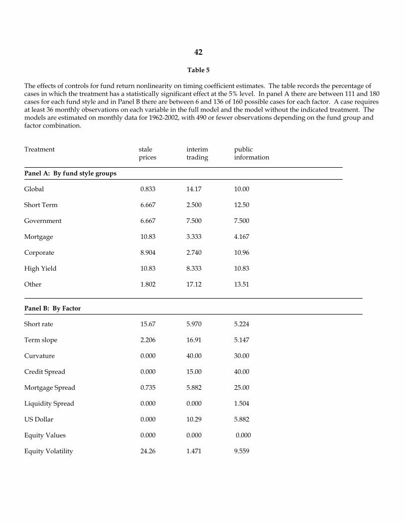
42 Table 5
The effects of controls for fund return nonlinearity on timing coefficient estimates. The table records the percentage of cases in which the treatment has a statistically significant effect at the 5% level. In panel A there are between 111 and 180 cases for each fund style and in Panel B there are between 6 and 136 of 160 possible cases for each factor. A case requires at least 36 monthly observations on each variable in the full model and the model without the indicated treatment. The models are estimated on monthly data for 1962-2002, with 490 or fewer observations depending on the fund group and factor combination. Treatment stale interim public prices trading information Panel A: By fund style groups Global 0.833 14.17 10.00 Short Term 6.667 2.500 12.50 Government 6.667 7.500 7.500 Mortgage 10.83 3.333 4.167 Corporate 8.904 2.740 10.96 High Yield 10.83 8.333 10.83 Other 1.802 17.12 13.51 Panel B: By Factor Short rate 15.67 5.970 5.224 Term slope 2.206 16.91 5.147 Curvature 0.000 40.00 30.00 Credit Spread 0.000 15.00 40.00 Mortgage Spread 0.735 5.882 25.00 Liquidity Spread 0.000 0.000 1.504 US Dollar 0.000 10.29 5.882 Equity Values 0.000 0.000 0.000 Equity Volatility 24.26 1.471 9.559

43

44

45

46

47

48

49

50


