
ePubWU Institutional Repository
Mehdi Amini and Tina Wakolbinger and Michael Racer and Mohammed G.Nejad
Alternative Supply Chain Production-Sales Policies for New ProductDiffusion: An Agent-Based Modeling and Simulation Approach
Article (Accepted for Publication)(Refereed)
Original Citation:
Amini, Mehdi and Wakolbinger, Tina and Racer, Michael and Nejad, Mohammed G.
(2012)
Alternative Supply Chain Production-Sales Policies for New Product Diffusion: An Agent-BasedModeling and Simulation Approach.
European Journal of Operational Research, 216 (2).
pp. 301-311. ISSN 0377-2217
This version is available at: https://epub.wu.ac.at/3304/Available in ePubWU: December 2011
ePubWU, the institutional repository of the WU Vienna University of Economics and Business, isprovided by the University Library and the IT-Services. The aim is to enable open access to thescholarly output of the WU.
This document is the version accepted for publication and — in case of peer review — incorporatesreferee comments. There are minor differences between this and the publisher version which couldhowever affect a citation.
http://epub.wu.ac.at/

1 | P a g e Amini, Wakolbinger, Racer & Nejad
Alternative Supply Chain Production-Sales Policies for New Product Diffusion: An Agent-Based Modeling and Simulation Approach
Mehdi Aminia,*, Tina Wakolbinger b, Michael Racer a, Mohammad G. Nejad c
a Department of Marketing and Supply Chain Management, The Fogelman College of Business and Economics,
The University of Memphis, Memphis, TN 38152, USA, [email protected]; http://fcbeold.memphis.edu/modules/general/Fc_facdetails.php?id=8&topic=bio.
b Institute for Transport and Logistics Management, WU, Vienna University of Economics and Business, Nordbergstraße 15/D/6/621 C, 1090 Vienna, Austria.
c School of Business Administration, Fordham University, New York, NY 10023, USA. *Corresponding author.
To appear in: European Journal of Operational Research, 216 (2012) 301-311.
Abstract
Applying Agent-Based Modeling and Simulation (ABMS) methodology, this paper
analyzes the impact of alternative production-sales policies on the diffusion of a new
product and the generated NPV of profit. The key features of the ABMS model, that
captures the marketplace as a complex adaptive system, are: (i) supply chain capacity is
constrained; (ii) consumers’ new product adoption decisions are influenced by marketing
activities as well as positive and negative word of mouth (WOM) between consumers; (iii)
interactions among consumers taking place in the context of their social network are
captured at the individual level; and (iv) the new product adoption process is adaptive.
Conducting over 1 million simulation experiments, we determined the “best” production-
sales policies under various parameter combinations based on the NPV of profit generated
over the diffusion process. The key findings are as follows: (1) on average, the build-up
policy with delayed marketing is the preferred policy in the case of only positive WOM as
well as the case of positive and negative WOM. This policy provides the highest expected
NPV of profit on average and it also performs very smoothly with respect to changes in
build-up periods. (2) It is critical to consider the significant impact of negative word-of-
mouth on the outcomes of alternative production-sales policies. Neglecting the effect of
negative word-of-mouth can lead to poor policy recommendations, incorrect conclusions
concerning the impact of operational parameters on the policy choice, and suboptimal
choice of build-up periods.
Keywords: Supply chain management, Agent-based simulation, New product diffusion, Word of mouth

2 | P a g e Amini, Wakolbinger, Racer & Nejad
1. Introduction
Decisions concerning effective supply chain production, sales and entry policies to introduce a
new product to the marketplace are critical and often difficult to make, requiring an in-depth
understanding of the underlying diffusion processes. Consequences of these supply chain
decisions and policies impact the financial livelihood of a company. The significance of
production, sales, and diffusion policies is indicated by the fact that average sales and profits
from new product introductions reach 32% of overall sales and 31% of overall profits of a firm
(Griffin, 1997; Hauser, Tellis, & Griffin, 2006). Capacity decisions are especially difficult for
innovative products with a short lifecycle (Kamath and Roy 2007).
The problems that arise when supply and demand processes are not properly understood
are highlighted by the cases of Tamagotchi and Playstation 3. Tamagotchi, the first virtual pet,
was introduced by Bandai in 1996. Due to extreme word-of-mouth (WOM), demand increased
very quickly and exceeded expectations and insufficient capacity led to lost sales; when Bandai
finally extended its capacity, demand declined (Higuchi & Troutt, 2004). While initial sales of
Sony’s Playstation 2 (PS2) were more than ten times that of the original PS’s introduction five
years earlier (New York Times, 2000), the launch of Playstation 3 (PS3) was not successful and
resulted in $1.8B annual loss in its game division and layoff of 3% of its workers (Los Angeles
Times, 2007).
The key objectives of this study are to advance the current literature on the interaction
between the diffusion processes of new products and supply chain production-sales decisions; to
compare the performance characteristics of three production-sales policies, myopic, build-up,
and build-up with delayed product roll-out, under restricted supply with positive and/or negative
WOM based on the net present value of profit generated; and to provide managerial
recommendations concerning the best production-sales policy and the optimal number of build-
up periods. To the best of our knowledge, there is no evidence in the published literature
focusing on the hybridization of new product diffusion and supply chain policies, where supply
chain capacity is limited; negative WOM is present; and consumers’ interactions are conducted
via a social network.
The study achieves these objectives by developing an agent-based simulation model
(ABMS) that considers the new product diffusion process as a complex adaptive system where:

3 | P a g e Amini, Wakolbinger, Racer & Nejad
(a) individual consumer decision is subjected to nonlinear interactions and positive and negative
WOM in the consumer social network; (b) the diffusion process is an adaptive system where the
current status of adoption throughout the social network is influenced by the adoption decisions
made in previous diffusion periods, the marketing activities, WOM, production capacity, and
carrying inventory; and (c) both consumer interactions and the diffusion process are considered
dynamic throughout the entire diffusion period. The remainder of this paper is organized as
follows. Section 2 provides a literature review. In section 3, we present the ABMS methodology;
introduce the model components; develop an ABMS model; sketch an ABMS algorithmic
design; and present our computational experimental design. In section 4, we discuss the
computational results and managerial implications. Finally, in section 5 we present summary,
conclusions, and potential extensions of this study.
2. Literature Review
Focusing on the demand side and ignoring the issues relevant to supply, the diffusion process of
new products has traditionally been analyzed in the marketing literature. Diffusion models for
single products as well as competitive products have been proposed (Yan & Ma, 2011).
Marketing and pricing strategies for new innovations were explored using optimal control theory
(Kamrad, et al., 2005). Empirical research determined the effect of interaction on product
diffusion and adoption (Emmanouilides & Davies, 2007) and the effect of advertising on
subscriber service adoption (Mesak, et al., 2011).
The majority of innovation diffusion models are based on the classical Bass model (Bass,
1969). Bass depicts the new product diffusion process using two parameters: marketing activity
and WOM among consumers (Mahajan, Muller, & Bass, 1990). Generally, Bass-type models
only consider the effect of positive WOM and assume unrestricted availability of supply.
Additionally, the outcomes of the diffusion process generated by these models are at the
aggregate market level (Bass, 1969, 2004). Capturing market effect, positive WOM, unrestricted
product supply and aggregate diffusion outcome allows modelers to model the new product
diffusion process in closed-formulation; and hence allows them to produce exact model
solutions.
The importance of analyzing diffusion processes while considering supply restrictions
was first discovered in the marketing science literature by Simon and Sebastian (1987), who
4 | P a g e Amini, Wakolbinger, Racer & Nejad
analyzed the diffusion of telephones in Germany. Based on insights by Simon and Sebastian
(1987), Jain et al. (1991) developed an extended Bass model that includes supply constraints.
They used the resulting model to forecast the demand of new telephones in Israel. Swami and
Khairnar (2006) developed a sales prediction model by extending the Bass model to include
supply constraints as well as an expiration date. They explicitly include the scarcity effect that
highlights that opportunities are more valuable when they are scarcer. Stonebraker and Keefer
(2009) suggest a methodology based on decision analysis to calculate potential demand for
supply constrained products.
While marketing literature focuses on developing supply restricted diffusion models to
improve sales forecasts, researchers in the operations literature concentrated on developing
supply-restricted diffusion models to enhance quality of capacity, production and sales decisions.
In the operations literature, Ho et al. (2002) relax the assumption that demand is given and
independent of capacity decisions. They developed an extended Bass model that includes
capacity constraints. Their model finds the optimal production and sales plans that maximize
profit during the new product’s life-cycle, spanning from one to two years. They determine that
delaying sales is never a beneficial policy. Kumar and Swaminathan (2003), however, who also
extend the Bass model to include supply constraints, show that delaying sales can be a beneficial
policy under certain conditions. They show that the build-up policy is robust and very close to
optimal on average, and under certain scenarios the myopic policy may deviate far from optimal.
Xiaoming et al. (2011) developed a supply restricted diffusion model that also includes negative
WOM from consumers who do not receive the product. Although the previous models
introduced in the literature offer valuable contributions in studying the dynamics of the supply or
demand side independently or simultaneously, they had their own limitations. First, these
models produce new product diffusion results at the aggregate level, ignoring the impact of
individual consumers on the diffusion process. Second, although critical, they do not consider the
effect of negative word-of-mouth (WOM) caused by consumers who buy the product but are not
satisfied with the quality of the product. Third, previous model developments ignore the
consumers social networks within which individual consumers interact.
More recently, studies have highlighted the importance of the relationship between
individual consumer behavior and aggregate market outcomes (Bass, 2004; Garcia, 2005;
Guenther, et al., 2010; Hauser, et al., 2006). These studies have shown that individual consumer

5 | P a g e Amini, Wakolbinger, Racer & Nejad
interactions, positive and negative, provide important insights about aggregate diffusion (Garber,
et al., 2004; Goldenberg, et al., 2007; Goldenberg, Libai, & Muller, 2002). They showed that
negative WOM not only impacts individual-level adoption, but it can also have a negative impact
on diffusion outcomes. Usually, only a small percentage of consumers report their complaints to
the firm; therefore, marketers can easily underestimate the presence of negative WOM in the
marketplace and its potential impact on new product diffusion. The most common sources of
negative WOM are known to be dissatisfied adopters or product rejecters. Regardless of the
source, due to the non-linear adaptive nature of negative WOM circulation, even a small
percentage of dissatisfied consumers can significantly reduce firms’ revenues. While Goldenberg
et al. (2007) highlighted the importance of negative WOM in the context of diffusion processes
without supply restrictions, models that studied optimal capacity and sales decisions in the
context of supply-restricted diffusion processes did not consider the effect of negative WOM
from dissatisfied consumers, at consumer or aggregate levels. Table 1 summarizes previous
literature.
Diffusion Without Capacity
Constraints Diffusion With Supply Constraints
Only Positive WOM
e.g. Bass (1969); Mahajan and Muller (1998); Goldenberg et al. (2002); Garberetal (2004); Vanden Bulte and Joshi (2007); Iyengar et al. (2008)
Simon and Sebastian (1987); Jan et al. (1991); Swami and Kairnar (2001); Kumar and Swaminathan (2003); Ho, Savin, and Terwiesch (2008)
Positive and Negative WOM
Goldenberg et al. (2007) (Xiaoming, et al., 2011)
Table 1. Literature Review
3. ABMS Model Development and Computational Experimental Design
While manufacturing and logistics operations can be characterized as complex (Nilsson and
Darley 2006), there are only few applications of complex systems methods in the area of
production and operations management (Baldwin, Allen, & Ridgway, 2010). A complex
adaptive system (CAS) is composed of interacting components and adapts to its changing
environment. In studying complex adaptive systems, simple interactions among components and
its environment might result in unpredicted complex patterns, referred to as emergence

6 | P a g e Amini, Wakolbinger, Racer & Nejad
phenomena. Modeling embedded complexities, including system dynamism, adaption, and
nonlinear interactions, approaches the limits of traditional modeling methods (Garcia, 2005;
North & Macal, 2007). Agent-based models provide valuable insights concerning tactical and
operational decisions in complex systems (Nilsson & Darley, 2006).
An agent-based model is built on the interactions between decision-makers as opposed to
an equation-based model that is constructed based on a set of equations that reflects observables
(Parunak, Savit, & Riolo, 1998). Relying on extensive computational experiments, Rahmandad
and Sterman (2008) conclude that deterministic models, differential equation models, and agent-
based models differ for several metrics including diffusion speed and peak load and that these
models respond differently to intervention policies, even when the base cases behave similarly.
Successful applications of ABMS include models to simulate the process of technological
innovation (Ma & Nakamori, 2004), technological market structure evolution in electricity
markets (Bunn & Oliviera, 2007), production strategies in the lumber industry (Yáñez, et al.,
2009), and distribution strategies of a novel biomass-fuel (Guenther, et al., 2010).
The marketplace under study resembles a complex adaptive system that is driven by
socially networked consumer interactions and, hence, can be best studied using an ABMS
(Miller & Page, 2007; North & Macal, 2007). ABMS allows us to capture: (a) consumers as
agents with three essential attributes: autonomy, interactivity, and bounded rationality; (b)
dynamic social network interactions among consumers; (c) the effect of marketing activities on
consumers; (d) positive and negative WOM between consumers; and (e) adoption status of
individual consumers as well as aggregate diffusion at the market level throughout the new
product diffusion process. As in Kumar and Swaminathan (2003), we assume that the
marketplace consists of a single firm that sells a new “generic “consumer product, price does not
impact a consumer’s buying decision, and consumers are engaged in a one-time purchase
decision.
In this section, we present discussions about the following topics: (3.1) consumers’ social
network attributes and adoption decision (3.2) alternative production-sales policies to study;
(3.3) NPV as the performance measurement applied for comparative analysis among alternative
production-sales policies; (3.4) ABMS algorithm developed and implemented for this study; and
(3.5) the ABMS computational experimental design.
7 | P a g e Amini, Wakolbinger, Racer & Nejad
3.1 Consumer Social Network and Adoption Decision
Interactions between consumers emerge in the context of their social networks. Social networks
provide the setting for individuals to interact and exchange information (Barabasi, 2002; Watts &
Strogatz, 1998). The structure of consumer social networks is not known with certainty
(Alderson, 2008; Watts & Dodds, 2007). A few recent studies that attempted to map large scale
social networks resulted in different network structures (Bampo, et al., 2008; Goldenberg, et al.,
2009). In the absence of empirical details about social network structure, we assume a random
network structure as a “null” hypothesis (Alderson, 2008).
A recent experiment found that the average number of consumers’ social ties is 25
(Goldenberg, et al., 2007). This number is in line with that found in a panel of 250,000 teenagers
by Tremor of P&G (McCarthy, 2007). Therefore, we assume that the average number of social
ties is 25. Similar to earlier studies (e.g., Goldenberg, et al., 2007; Kumar & Swaminathan,
2003), we model a market of 3,000 consumers. To discover whether a larger size market may
impact the simulation results, we repeated experimental designs on larger networks. The analysis
showed no significant differences in the simulation results; hence, we chose a random network
structure linking 3,000 consumers for all designed experiments. We terminated an experiment
when 95% of 3,000 potential consumers made adoption decisions.
We now describe the decision-making process applied by socially-networked consumers
regarding product adoption or rejection at each period. We describe consumers’ decision-making
process in the cases, where both positive and negative WOM are present. For the cases with only
positive WOM product rejecters and dissatisfied adopters,were removed from the model.
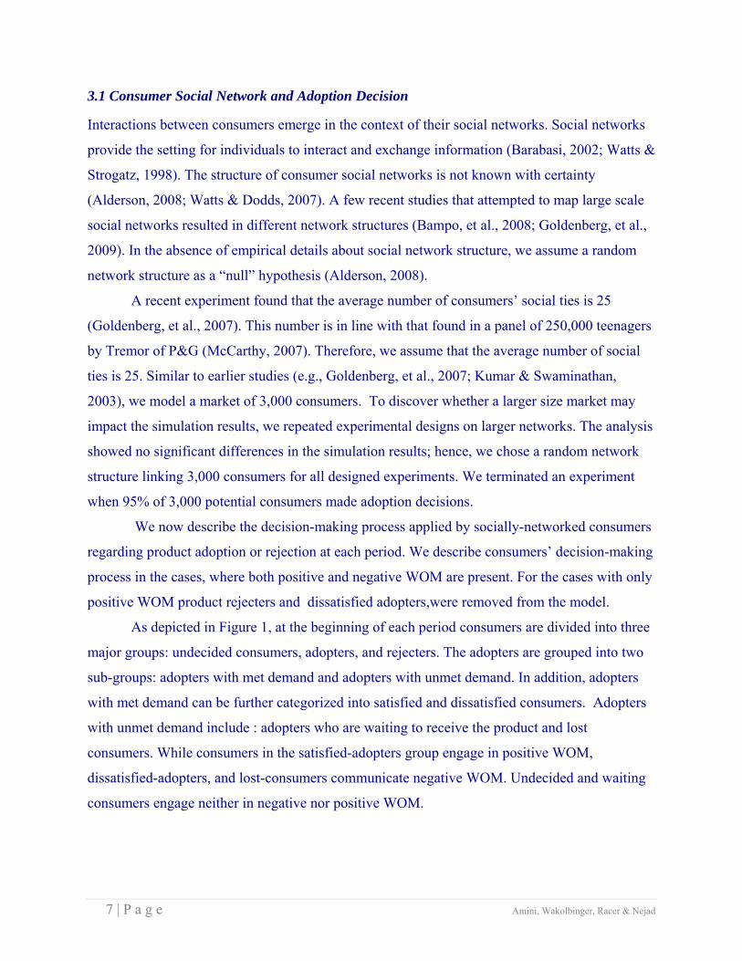
As depicted in Figure 1, at the beginning of each period consumers are divided into three
major groups: undecided consumers, adopters, and rejecters. The adopters are grouped into two
sub-groups: adopters with met demand and adopters with unmet demand. In addition, adopters
with met demand can be further categorized into satisfied and dissatisfied consumers. Adopters
with unmet demand include : adopters who are waiting to receive the product and lost
consumers. While consumers in the satisfied-adopters group engage in positive WOM,
dissatisfied-adopters, and lost-consumers communicate negative WOM. Undecided and waiting
consumers engage neither in negative nor positive WOM.
8 | P a g e Amini, Wakolbinger, Racer & Nejad
Figure 1. Consumer New Product Adoption Status
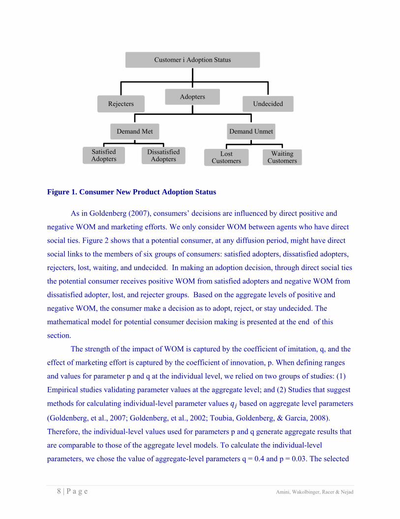
As in Goldenberg (2007), consumers’ decisions are influenced by direct positive and
negative WOM and marketing efforts. We only consider WOM between agents who have direct
social ties. Figure 2 shows that a potential consumer, at any diffusion period, might have direct
social links to the members of six groups of consumers: satisfied adopters, dissatisfied adopters,
rejecters, lost, waiting, and undecided. In making an adoption decision, through direct social ties
the potential consumer receives positive WOM from satisfied adopters and negative WOM from
dissatisfied adopter, lost, and rejecter groups. Based on the aggregate levels of positive and
negative WOM, the consumer make a decision as to adopt, reject, or stay undecided. The
mathematical model for potential consumer decision making is presented at the end of this
section.
The strength of the impact of WOM is captured by the coefficient of imitation, q, and the
effect of marketing effort is captured by the coefficient of innovation, p. When defining ranges
and values for parameter p and q at the individual level, we relied on two groups of studies: (1)
Empirical studies validating parameter values at the aggregate level; and (2) Studies that suggest
methods for calculating individual-level parameter values based on aggregate level parameters
(Goldenberg, et al., 2007; Goldenberg, et al., 2002; Toubia, Goldenberg, & Garcia, 2008).
Therefore, the individual-level values used for parameters p and q generate aggregate results that
are comparable to those of the aggregate level models. To calculate the individual-level
parameters, we chose the value of aggregate-level parameters q = 0.4 and p = 0.03. The selected
Customer i Adoption Status
Rejecters UndecidedAdopters
Demand Met
Satisfied Adopters
Dissatisfied Adopters
Demand Unmet
Lost Customers
Waiting Customers

9 | P a g e Amini, Wakolbinger, Racer & Nejad
p and q represent average values considered for a typical product (Jiang, Bass, & Bass, 2006;
Sultan, Farley, & Lehmann, 1990). We then transformed the values of aggregate-level parameter
q to individual-level parameter by dividing it by the number of links of each individual (i.e.,
25). The value of parameter p will be the same for both individual-level and aggregate-level
models (Goldenberg, et al., 2002; Toubia, et al., 2008).
Figure 2. Word-of-Mouth through Direct Social Ties to Members of Other Consumer Groups
Influenced by WOM and marketing efforts, potential consumers decide to adopt the
product, reject it, or stay undecided. While positive WOM communicated with the undecided
consumer through his/her social ties and marketing effort encourage undecided consumers to
adopt the new product, negative WOM discourages potential adopters from adopting. The impact
of negative WOM on an undecided consumer is calculated by identifying the number of
rejecters, dissatisfied adopters, or lost consumers among her/his social ties. L(i)+ is the index set
of consumers with whom consumer i has social ties and who are sources of positive WOM
(satisfied adopters). L(i)– is the index set of consumers with whom consumer i has social ties and
who are sources of negative WOM.
Generally, the marketing literature suggests that negative WOM has a greater impact on
potential consumers’ adoption decisions than positive WOM (e.g., Arndt, 1967; Harrison-
Walker, 2001) due to two main reasons: (1) People assign more weight to negative WOM than to
positive WOM (Hart, Heskett, & Sasser, 1990; Mizerski, 1982) (2) A dissatisfied consumer talks
Satisfied Adopters
Dissatisfied Adopters Rejecters & Lost Consumers
Undecided &Waiting Consumers
Potential Consumer
Positive WOM
No WOM
Negative WOM
Negative WOM
10 | P a
to more p
earlier stu
TARP, 1
T
determin
internal p
network
In
positive i
positive W
of these t
from neit
product o
influence
N
from diss
Assumin
probabili
product o
product f
T
period tn
or neithe
probabili
positive
a g e
people than a
udies and ac
982, 1986),
To determine
ne the probab
positive WO
links with co
, 1
n equation [1
impact of ad
WOM from
two terms in
ther advertis
of the two te
e from adver
Next, we dete
satisfied ado
, 1
ng that the im
ity of consum
of (1 – M * q
from 1, resul
To calculate t
now may be e
er. Hence,
) ,
ity of being
. We allow
WOM to a
a satisfied co
ccepted indu
he relative p
e the adoptio
bility of cons
OM,
onsumer i as
1 – 1 – ∏
1], (1 – p) in
dvertisement
any of the s
ndicate the pr
sement or sat
erms from 1 i
rtisement or
ermine the p
opters, produ
1 – ∏ 1 M
mpact of neg
mer i not rec
qj) for all dis
lts in the pro
the transition
exposed to p
the probabil
also for on
influenced
a proportion
adopt the pr
onsumer (An
stry practice
power of neg
n status of a
sumer i to be
, received f
s follows:
∏ 1 ,
ndicates the p
t. In addition
atisfied adop
robability of
tisfied consu
indicates the
satisfied ado
robability of
uct rejecters,
M , wh
ative WOM
ceiving any n
ssatisfied con
obability of c
n probability
positive influ
lity of being
nly negative
by both pos
n of αi of the
roduct, and
nderson, 199
es (Goldenbe
gative WOM
an undecided
e influenced
from satisfie
where
probability th
n, the probab
pter j with di
f consumer i
umers with d
e probability
opters with d
f negative W
and lost con
here L
is M times t
negative WO
nsumers j w
consumer i r
y, we need to
uence, negat
g exposed t
e WOM (1
sitive and ne
e consumers
(1 - αi) to
98; TARP, 1
erg, et al., 20
M to positive
d consumer i
by either ex
ed consumer
hat consume
bility of con
irect social l
i not receivin
direct social
y of consume
direct social
WOM
nsumers as f
the positive
OM at diffusi
ith direct soc
eceiving neg
o recognize
tive influenc
to only posi
-
egative WO
that are infl
o reject. T
Amini, Wa
982, 1986).
007; Hart, et
WOM is fix
i in period tn
xternal adver
s having dire
er i is not inf
sumer i not r
link is (1 – qj
ng any positi
links. Subtra
er i receiving
links.
, received
follows:
WOM, in eq
ion period tn
cial links. Su
gative WOM
that a potent
ce, both posi
itive WOM
) .
M is measu
luenced by b
The normaliz
kolbinger, Racer &
In line with
t al., 1990;
xed at 2.
now, first we
rtisement or
ect social
[1]
fluenced by t
receiving
qj). The produ
ive influence
acting the
g positive
d by consum
[2]
quation [2] th
now is the
ubtracting th
M.
tial consume
tive and neg
is given by
In addition
ured by
both negative
zation facto
& Nejad
e
by
the
uct
e
mer i
he
his
er i at
gative
y (1 -
n, the
e and
or, αi,

11 | P a g e Amini, Wakolbinger, Racer & Nejad
indicating the ratio of positive WOM over the total WOM influence received by consumer i, both
positive and negative is calculated by:
,
, , [3]
Given this normalization factor, the probabilities of product adoption, , , rejection,
, , or wait-to-decide, , , for an undecided consumer i at period tnow are determined
by:
, 1 , , αi , , , [4]
, 1 , , 1 αi , , , [5]
, 1 , 1 , . [6]
Equations [4], [5], and [6] would add up to 1. Given d as the percentage of dissatisfied
consumers, consumer i becomes a satisfied adopter with probability of , , a dissatisfied
adopter with probability of 1 , , and a rejecter with probability of , .
Consumer i in period tnow might stay undecided with probability of , .
3.2 Production-Sales Policies to Study
In this study, we compare performance characteristics of three alternative production-sales
policies: myopic, build-up, and build-up with delayed roll-out (build-up 2). As Kumar and
Swaminathan (2003) point out, while computing optimal production-sales plans explicitly is
quite difficult, the myopic and build-up policies have simple, intuitive structures and could be
used as heuristics to closely estimate “optimal” plans. We consider three alternatives using
ABMS, rather than using a closed-formulation. Table 2 shows the characteristics of the three
production-sales policies with respect to the time period when production, marketing activities
and sales start.
Policy Start of Production Start of Marketing Activities Start of Sales
Myopic Period 1 Period 1 Period 1
Build-up Period 1 Period 1 Period t>1
Build-up 2 Period 1 Period t>1 Period t>1
Table 2. Policy Comparisons

12 | P a g e Amini, Wakolbinger, Racer & Nejad
In the myopic policy, the company begins producing, promoting and selling the product
in period 1. In each period it sells as much as possible. If a firm applies the build-up policy,
production and promotion begins simultaneously in period 1. Marketing activities during the
build-up period will generate some demand, but the product is not available for sales. Hence,
interested consumers must wait until the build-up period is completed, or withdraw.. Thus,
during the build-up period, no revenue is realized, but the variable, inventory holding, and
consumer waiting costs would occur, resulting in negative NPV profit. After the build-up, the
company sells as much as possible. For the build-up policy with delayed roll-out (build-up 2),
the company begins producing in period 1, but marketing and product sales start after the initial
build-up period is passed. In build-up 2, no demand is generated during the build-up period and
so no consumers are lost. An example of this is the delayed roll-out of Playstation 2 by Sony
(Kumar & Swaminathan, 2003). The ABMS parameters for the production-sales policies are
selected as follows. Assuming that the overall diffusion period is between one to two years (with
each period lasting two to four weeks), the number of periods is estimated to be 30.
Accordingly, the production capacity per period is set to 100. Regardless of the policy ,
production begins in period 1. The decision concerning production quantity is made based on
expected demand. As long as the percentage of consumers who made adoption decisions is
below 84% of the market potential (3,000 consumers), the production quantity is equal to the
production capacity. After this threshold is reached, the number produced is set to the demand in
the previous period. The choice of 84% was made due to the fact that the last 16% of the market
potential who adopt a new product, referred to as laggards, are slow in adopting (Rogers, 2003).
Utilization of the maximum capacity during this period might introduce carrying inventory and,
hence, increase total costs. In addition to the aforementioned parameters, performance
characteristics of build-up 1 and build-up 2 are impacted by the number of build-up periods. The
range of build-up periods in the designed simulation experiments is between 1 and 12.
3.3 NPV Calculation
Performance characteristics of different production-sales policies are compared based on the
NPV of the overall profit they generate throughout the diffusion period. Each policy is initiated
with a negative net present value, reflecting fixed cost. To determine net profit for a policy in

13 | P a g e Amini, Wakolbinger, Racer & Nejad
each diffusion period, the total of relevant costs including variable costs, carrying inventory
costs, and consumer waiting costs is subtracted from the current period gross revenue (unit price
times units sold). Next, using a discount rate, the NPV of the profit generated for the period is
determined. Finally, the NPV of the period under consideration is added to the total net present
value.
3.4 The ABMS Algorithm in Brief
In this sub-section, we present the ABMS simulation algorithm for the myopic policy. The
supplement details an ABMS pseudo-algorithm developed and implemented for this study. The
ABMS algorithm for all alternatives is described in the supplement.
Regardless of the policy under consideration, at the beginning of each period, the
available supply includes the carrying inventory from the previous period and the current
production. Before continuing the process, we allocate the current supply to meet the demand of
waiting consumers. If possible, we meet the demand of all waiting consumers. Otherwise, the
remaining waiting consumers with unmet demand have may keep waiting or withdraw. Any time
a waiting consumer leaves, potential revenue is lost. After the waiting consumers are resolved,
we might have exhausted product supply. If not, the diffusion process continues with some
positive level of carrying inventory. As we continue the process, we apply equations [1] through
[6] to determine the adoption status of each undecided consumer. If an individual consumer
decides to adopt the product, then depending on the availability of supply, his/her demand could
be met or the consumer must decide whether to join the waiting consumers group or completely
withdraw.
3.5 The ABMS Computational Experimental Design
Given this set of issues of interest – type of WOM and build-up decisions – a total of six
simulation scenario models were developed for the computational study. Figure 3 shows the
classification of the six different simulation scenario models.
The selected parameter values, ranges, and adoption sources used in experiments with
the six ABMS models are summarized in Table 3. The purpose of selecting parameters from
previous papers was to have a basis for comparison of the results produced by our ABMS
modelling effort. The flexibility embedded in the current ABMS models readily allows
consideration of other parameter sets. These parameters are organized in four subsets: consumer

14 | P a g e Amini, Wakolbinger, Racer & Nejad
social network; new product diffusion; production-sales policies; and simulation termination
criteria.
Figure 3. The Six ABMS Simulation Scenarios (Models)
Given a simulation model in Figure 3 and a selected parameter combination, we complete the
simulation experiment as follows. First, we generate five random social networks, each
including 3,000 consumers. Using each of the five networks, we replicate simulation of the new
product diffusion process 10 times, each with a new random number stream. In total, for each
parameter combination applied to a given simulation scenario model, we generate 50 sets of
simulation results. The number of replications per experimental cell was determined based on a
steady-state analysis, which indicated that the minimum number of replications necessary for
stability is 50.
While models 1 and 2 each include 432 parameter combinations, models 3 to 6 each include
5,184 parameter combinations. Considering all six simulation scenario models and parametric
combinations, the computational experiments produced results for a total of 1,080,000
experiments. For each scenario, a simulation algorithm was developed and implemented. The
algorithms were developed on a standard Dell desktop (Xeon, CPU 3.2 GHz, and 2.00 GB of
RAM), Microsoft Windows XP Professional 2002 operating system, in Compaq Visual Fortran
environment. All computational experiments were conducted in the same environment.

15 | P a g e Amini, Wakolbinger, Racer & Nejad
ABMS Simulation Model Parameters Parameters Parameter Value
or Range Selection Sources
Market size 3,000 Kumar and Swaminathan (2003) Average number of social ties per consumer 25 Goldenberg et al. (2007) Coefficient of innovation 0.03 Sultan et al. (1990) Coefficient of imitation 0.40 Sultan et al. (1990) Percentage of dissatisfied adopters 5 % Goldenberg et al. (2007) Relative power of negative WOM to positive WOM (M) 2 Goldenberg et al. (2007); Hart et al.
(1990); TARP (1982); TARP (1986) Supply chain capacity per period 100 Kumar and Swaminathan (2003) Unit capacity fixed cost 10 Above Unit variable cost 1 Above Unit backlogging cost per period 0.01, 0.005, and
0.001. Above
Unit selling price 1.1, 1.2 and 1.3 Above Unit inventory holding cost 0.01, 0.005 and
0.001 Above
Discount rates 0.01, 0.005, 0.003 and 0 Above
Percentage of backlogged demand 0, 0.5, 0.8, and 1 Above Build-up periods 0-12 Above Percentage of market adoption at which supply chain capacity is adjusted to previous period demand
84 % Rogers (2003)
Percentage of consumers who made adoption decision at which simulation is terminated 95 % Goldenberg et al. (2007); Rogers (2003)
Table 3. Parameter Choices for ABMS Computational Experiments
4. Analyses of Simulation Results
In this section, we present the results. Based on the experimental design, we study the three
production-sales policies described in the previous sections. The performance characteristics of
the three policies are compared based on the net present value of profit generated over the
diffusion process. In a complex system such as the one modelled, it is vital to make sure that the
simulation performs as anticipated. To ensure this, we evaluated a set of pilot runs in detail.
Outcomes such as profit were evaluated with respect to changes in each of the input parameters.
In addition, analyzing diffusion processes with only positive WOM allowed us to compare our
results to those in Kumar and Swaminathan (2003).
16 | P a g e Amini, Wakolbinger, Racer & Nejad
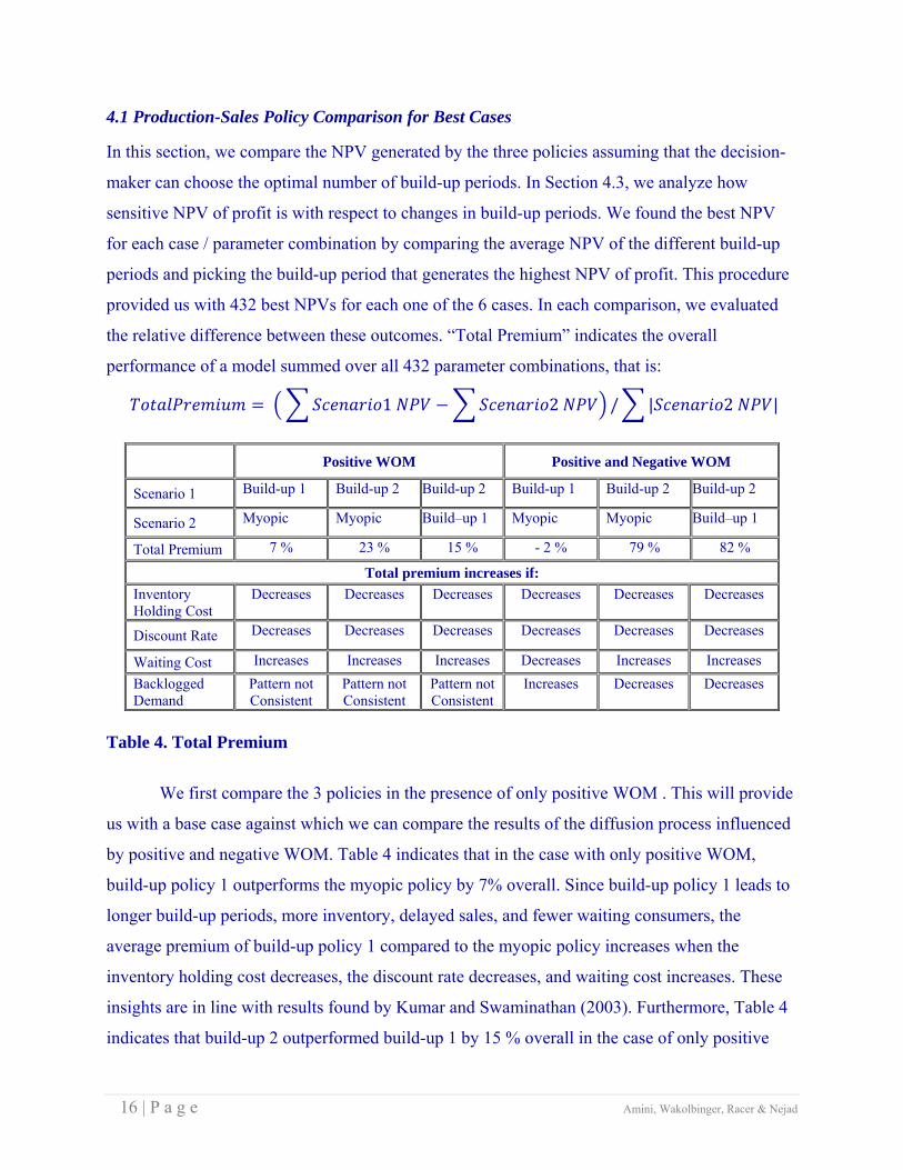
4.1 Production-Sales Policy Comparison for Best Cases
In this section, we compare the NPV generated by the three policies assuming that the decision-
maker can choose the optimal number of build-up periods. In Section 4.3, we analyze how
sensitive NPV of profit is with respect to changes in build-up periods. We found the best NPV
for each case / parameter combination by comparing the average NPV of the different build-up
periods and picking the build-up period that generates the highest NPV of profit. This procedure
provided us with 432 best NPVs for each one of the 6 cases. In each comparison, we evaluated
the relative difference between these outcomes. “Total Premium” indicates the overall
performance of a model summed over all 432 parameter combinations, that is:
1 2 / | 2 |
Positive WOM Positive and Negative WOM
Scenario 1 Build-up 1 Build-up 2 Build-up 2 Build-up 1 Build-up 2 Build-up 2
Scenario 2 Myopic Myopic Build–up 1 Myopic Myopic Build–up 1
Total Premium 7 % 23 % 15 % - 2 % 79 % 82 %
Total premium increases if: Inventory Holding Cost
Decreases Decreases Decreases Decreases Decreases Decreases
Discount Rate Decreases Decreases Decreases Decreases Decreases Decreases
Waiting Cost Increases Increases Increases Decreases Increases Increases Backlogged Demand
Pattern not Consistent
Pattern not Consistent
Pattern not Consistent
Increases Decreases Decreases
Table 4. Total Premium
We first compare the 3 policies in the presence of only positive WOM . This will provide
us with a base case against which we can compare the results of the diffusion process influenced
by positive and negative WOM. Table 4 indicates that in the case with only positive WOM,
build-up policy 1 outperforms the myopic policy by 7% overall. Since build-up policy 1 leads to
longer build-up periods, more inventory, delayed sales, and fewer waiting consumers, the
average premium of build-up policy 1 compared to the myopic policy increases when the
inventory holding cost decreases, the discount rate decreases, and waiting cost increases. These
insights are in line with results found by Kumar and Swaminathan (2003). Furthermore, Table 4
indicates that build-up 2 outperformed build-up 1 by 15 % overall in the case of only positive

17 | P a g e Amini, Wakolbinger, Racer & Nejad
WOM. The average premium of build-up 2 increases when the inventory holding cost decreases,
the discount rate decreases, and the waiting cost increases, indicating that build-up 2 leads on
average to delayed sales, more inventory, and fewer waiting consumers than build-up 1.
The trends in Table 4 are worth noting. Not surprisingly, total premiums of build-up 1
decrease as holding costs increase. Since any build-up policy will tend to hold inventory longer
than a myopic policy, the build-up policy becomes more attractive as holding costs decrease. In a
similar vein, build-up 2 gains in preference on build-up 1 as holding costs decrease: the benefits
of early marketing with respect to inventory are lessened.
A similar pattern holds for the discount rate. Across the board, we note an increase in the
total premiums, as the discount rate decreases. Models that tend to hold more inventory (build-up
vs. myopic) or market later (build-up 2 vs. build-up 1) benefit greatly when penalized less for
those holdings. This highlights the importance of inventory management.
In the case of only positive WOM, total premiums increase with an increase in waiting
costs, for build-up 1 vs. myopic. This pattern suggests that the availability of inventory provided
by an early build-up is rewarded significantly as it will reduce the number of those who have to
wait. Interestingly, total premiums also increase, for build-up 2 vs. build-up 1. This result
suggests that build-up 2 leads to fewer waiting customers, since marketing is delayed.
The impact of a change in waiting costs is not quite as clear in the presence of both
positive and negative WOM, and it is helpful to consider this in conjunction with backlogged
demand. Note that negative WOM is more likely when a customer must wait. As a result,
backlogged demand will impact future sales. When comparing build-up 1 to myopic, we actually
see a decrease in total premiums when the waiting costs increase. This accentuates the
importance of considering negative WOM, as we observe here that decreased waiting costs lead
to a more significant advantage for the build-up case. (Note that this is contrary to the PWOM
case.) This indicates that the impact of backlogged customers plays a larger role in customer
demand (and hence, profits) with the longer wait that is inherent in the myopic case. Due to the
delayed marketing that accompanies build-up 2, total premiums still tend to increase vs. build-up
1, as waiting costs increase, as was seen in the PWOM environment. This indicates the value of
lagging the marketing effort.
The most complex results occur when studying the impact of backlogged demand. When
there is only positive WOM, there is no consistent pattern. So, even though backlogged demand
18 | P a g e Amini, Wakolbinger, Racer & Nejad
produces a wait, the fact that there are also holding costs and delayed profits leads to too many
trade-offs among the elements to identify a strict relationship.
This is not the case, however, in the presence of negative WOM. In this environment,
backlogs lead to less satisfied customers. In the comparison of build-up 1 vs. myopic, we see this
increased wait enhances the position of building-up prior to product launch. And comparing
build-up 2 vs. build-up 1, it is notable that the decreased backlog is more beneficial to build-up 2,
again highlighting the value of not proceeding too soon to generate customer interest,
particularly, when the backlogs are manageable.
Comparing the cases where we allow only for positive WOM and the cases where we
allow for positive and negative WOM, we see that ignoring negative WOM can lead to wrong
recommendations. While we see that in the case with only positive WOM, build-up 1 is better
than myopic overall as the model by Kumar and Swaminathan (2003) indicates, the myopic
policy performs better than build-up 1 overall in the case of positive and negative WOM as the
model by Ho et al. (2002) suggests. Furthermore, inconsideration of negative WOM can lead to
wrong conclusions concerning the impact of operational parameters on policy choice. An
increase in waiting costs increases the total premium of build-up 1 compared to the myopic
policy in the case with only positive WOM, while it decreases the total premium in the case with
positive and negative WOM.
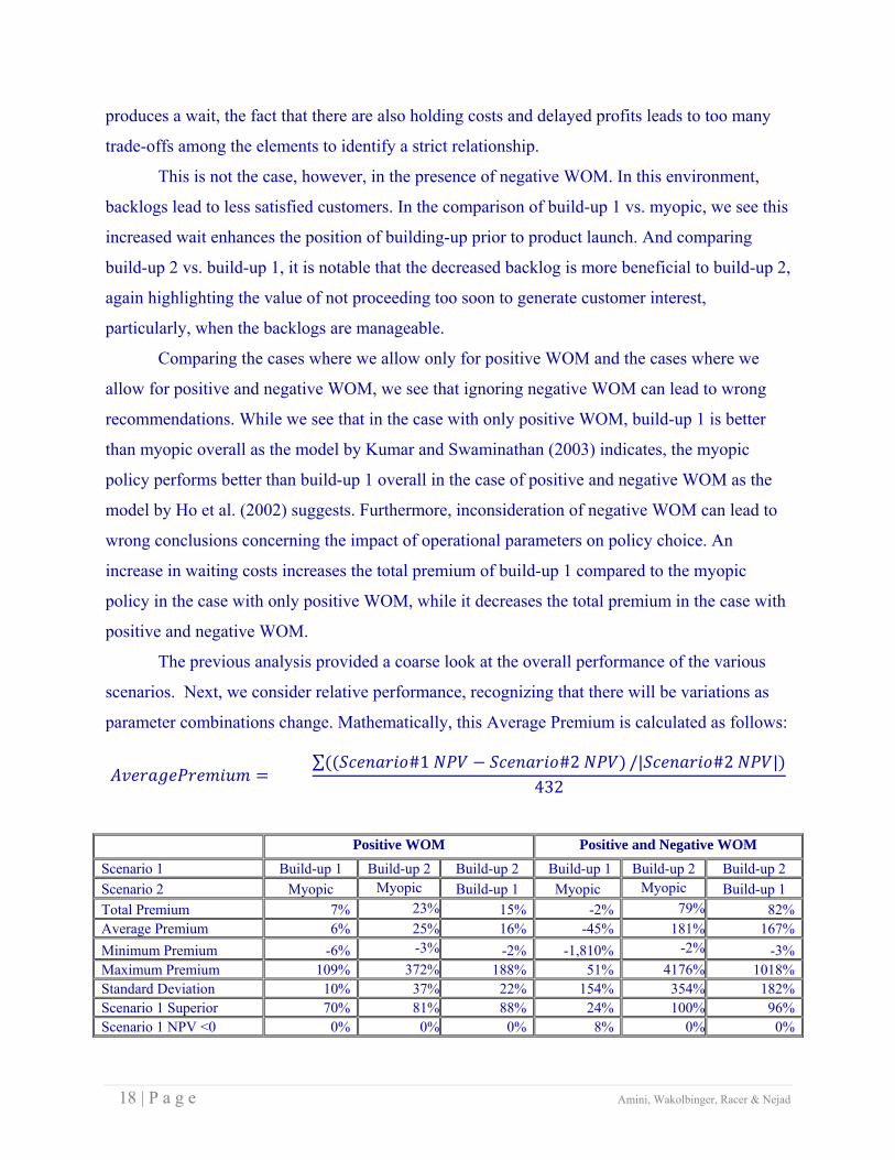
The previous analysis provided a coarse look at the overall performance of the various
scenarios. Next, we consider relative performance, recognizing that there will be variations as
parameter combinations change. Mathematically, this Average Premium is calculated as follows:
∑ #1 #2 /| #2 |
432
Positive WOM Positive and Negative WOM Scenario 1 Build-up 1 Build-up 2 Build-up 2 Build-up 1 Build-up 2 Build-up 2 Scenario 2 Myopic Myopic Build-up 1 Myopic Myopic Build-up 1 Total Premium 7% 23% 15% -2% 79% 82%Average Premium 6% 25% 16% -45% 181% 167%Minimum Premium -6% -3% -2% -1,810% -2% -3%Maximum Premium 109% 372% 188% 51% 4176% 1018%Standard Deviation 10% 37% 22% 154% 354% 182%Scenario 1 Superior 70% 81% 88% 24% 100% 96%Scenario 1 NPV <0 0% 0% 0% 8% 0% 0%

19 | P a g e Amini, Wakolbinger, Racer & Nejad
Table 5. Policy Comparisons
Table 5 indicates that there is a clearer relationship between total and average premiums
in the positive WOM cases, than in the cases involving both positive and negative WOM. This
would suggest that, when only positive WOM is a factor, both methods tend to perform similarly
in all cases; however, when both positive and negative WOM are in play, one model
significantly outperforms the other in some cases, and is slightly outperformed by the second
model in others.
This fact is evidenced when we look at the Minimum and Maximum lines. For instance,
when positive and negative WOM are present, the largest relative gain for the myopic case is
1,810 %, while the largest relative gain for build-up 1 is only 51%. The fact that the average
premium is so much smaller than the total premium reveals that such extremes are very common
in this instance. For the case of only positive WOM comparing build-up 1 and myopic policy we
see that while the minimum is -6% and the maximum is 109%; the average premium and the
total premium are fairly close, demonstrating that extreme differences are relatively rare. It is
also noteworthy to consider the volatility. When only positive WOM is evident, the standard
deviation of the relative performances is 10-37%. Compared to the averages, these are not at all
small, suggesting that one model does not completely dominate the other over all 432 scenarios.
This unpredictability is even more pronounced when both positive and negative WOM are in
play.
The volatility of the system as a function of the parameters is a critical issue. As noted
on Table 5, there is quite significant variability in relative performance. “Scenario 1 Superior”
indicates the percentage of the 432 combinations in which Scenario 1 outperformed Scenario 2.
In the case of PWOM, Build-up 1’s NPV exceeds that of the myopic scenario in 70% of the
cases. And as noted in “NPV<0”, there are no instances in which the NPV of Scenario 1 was
negative. A similar result is true for the comparison of the two build-up policies. The NWOM
case shows a slightly more challenging picture. Although build-up 1 again outperformed the
myopic policy, there were negative NPVs recorded in 8% of the scenarios.
The most striking feature of Table 5 is with respect to the standard deviation. In the
presence of only PWOM, results are as expected, and variability is fairly slight. On the contrary,
when both positive and negative WOM are present, there is a tremendous amount of variability.
This indicates how operational changes might have unintended effects. Front end production,

20 | P a g e Amini, Wakolbinger, Racer & Nejad
which increases holding costs, could at the same time reduce backlogged demands and its
negative impacts. However, front end production also delays any influences of WOM, which
influences the growth of demand throughout the process. The impact of these interwoven
influences is evidenced in the standard deviation of NPV.
4.2 Impact of Negative WOM
The introduction of negative WOM reduces the NPV of profit for all 3 policies. It reduces the
NPV of profit overall by 44 % for the myopic policy, 48 % for build-up 1, and 19 % for build-up
2.The reduction is strongly impacted by the consumers’ willingness to wait. If consumers are
likely to continue to wait for an out-of-stock product, results are very predictable, but as that
likelihood decreases, the results are much more variable.
Goldenberg et al. (2007) finds that for every percentage increase in consumer
dissatisfaction, the NPV of diffusion outcomes drops by 1.8%. The reduction in NPV of profit
that we describe in this paper is much larger than 1.8%. The model of Goldenberg et al. (2007)
differs from the model described in this paper in two major ways: it describes a diffusion process
that is not restricted by supply constraints and the consumer network is modelled using a small-
world network. This indicates that supply restrictions and network structure have the potential to
further increase the negative impact of negative WOM. It also highlights the importance of
further analyzing the impact of network structure on the diffusion process.
Managerial Implications: Managers can easily underestimate the presence of negative
WOM since only a small percentage of consumers report their complaints to the firm. The
numerical analysis highlights the importance of estimating the volume and frequency of negative
WOM, especially for managers that are faced with limited product supply and consumers that are
not willing to wait. Not considering negative WOM can lead to wrong policy recommendations
and misleading conclusions concerning the impact of operational parameters.
4.3 Effect of Build-Up Period Selection
We consider the issue of selecting the best build-up period, not a simple task. This might
be difficult to achieve. Therefore, we now suggest how sensitive the average NPV of profit is
with respect to the build-up periods in scenario models 3-6. To illustrate the point, in Figure 4 we
show the impact of build-up period selection for a single demonstration case for each of the

21 | P a g e Amini, Wakolbinger, Racer & Nejad
build-up models. What is of interest is the magnitude of the change in NPV as the number of
build-up periods is increased.
Figure 4. Effect of Build-up Period Selection
In scenario model 3 (build-up policy 1 with positive WOM), average NPV of profit is
pretty stable for build-up periods up to 7 with tradeoffs on lost sales and holding costs.
‐2000
0
2000
1 2 3 4 5 6 7 8 9 10 11 12
Ave ra
ge NPV
($)
#Build‐up Periods
Model 3 A Demonstration Case
0
50
1 2 3 4 5 6 7 8 9 10 11 12
Stan
dard Deviation
(NPV
)
#Build‐up Periods
Model 3 A Demonstration Case
‐1000
‐500
01 2 3 4 5 6 7 8 9 10 11 12
Ave ra
ge NPV
( $)
#Build‐up Periods
Model 4 A Demonstration Case
0
10
20
1 2 3 4 5 6 7 8 9 10 11 12
Stan
dard Deviation
(NPV
)
#Build‐up Periods
Model 4A Demonstration Case
0
100
200
300
1 3 5 7 9 11
Average
NPV
($)
#Build‐up Periods
Model 5A Demonstration Case
0
2
4
1 2 3 4 5 6 7 8 9 10 11 12Stan
dard Deviation
(NPV
)
#Build‐up Periods
Model 5 A Demonstration Case
‐200
0
200
1 2 3 4 5 6 7 8 9 10 11 12
Average
NPV
($)
#Build‐up Periods
Model 6 A Demonstration Case
0
50
1 2 3 4 5 6 7 8 9 10 11 12
Stan
dard Deviation
(NPV
)
#Build‐up Periods
Model 6A Demonstration Case

22 | P a g e Amini, Wakolbinger, Racer & Nejad
However, for build-up periods above 7, average NPV drops quickly and standard deviation
increases dramatically. As indicated in the examples, each model suggests a different sensitivity
to build-up period selection. This underscores the importance of management being well-tuned
to the implications of selection. Of the parameters under the control of management, the most
sensitive one appears to be the selection of the length of the build-up period. In addition, the
choice of build-up periods also affects the variability, and will play an important role in final
NPV of profit.
Managerial Implications: Choice of the number of build-up periods is a critical
management tool, particularly when considered along with the advertising strategy. A
reasonable build-up period can increase stock availability – lessening the likelihood of stock-outs
and rejected consumers once the product is launched. Consequently, NPV of profit can be
increased significantly. However, there are also disadvantages to long build-ups. When negative
WOM is present for build-up 1, consumers who receive advertising and want to buy the product
before the product is launched can become adverse voices. In addition, uncertainty in the NPV
tends to increase with longer build-up periods.
4.4 Production-Sales Policy Summary
At a significance level of 5%, an ANOVA was conducted to determine whether mean NPVs of
the three production-sales policies are significantly different. The results indicate statistical
significance with F(3,1724) = 407.21, p < 0.0001. Also, a post-hoc Tukey’s pairwise mean
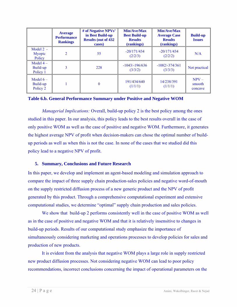
comparison was applied to rank the three policies. Tables 6.a and 6.b provide a brief summary of
the findings for the three policies investigated. When rankings are shown, ‘1’, ‘2’ and ‘3’
indicate the best, second best, and worst performing policies, respectively. Column 1 indicates
the general performance over all 432 scenarios. Column 2 identifies the number of scenarios in
which a negative NPV resulted when the best build-up period is chosen; this and column 3
summarize results for the best-build-up case – column 3 shows the minimum, average, and
maximum NPV over the 432 scenarios. If the best build-up period is not selected, then we must
consider column 4, which indicates the range of values resulting. Finally, column 5 summarizes
the implications of the number of build-up periods for each model.

23 | P a g e Amini, Wakolbinger, Racer & Nejad
Average
Performance Rankings
# of Negative NPVs in Best Build-up
Results (out of 432 cases)
Min/Ave/Max Best Build-up
Results (rankings)
Min/Ave/Max Average Case
Results (rankings)
# of Build-up Periods
Model 1 - Myopic 3 0 45/307/572
(2/3/3) 45/307/572
(2/2/2) N/A
Model 3 – Build-up Policy 1
2 36 -468/431/676 (3/2/2)
-727/187/391 (3/3/3)
NPV - very sensitive
Model 5 – Build-up Policy 2
1 0 444/568/785 (1/1/1)
46/336/665 (1/1/1)
NPV – smooth concave
Table 6.a. General Performance Summary Under Positive WOM
In practice, when only PWOM is considered, it appears that build-up 2 is the most stable
policy. Among the best performers, losses are avoided in all instances. The range of NPV’s is
fairly small, 341 (785-444). In all comparisons (min, max, and average), build-up 2 dominates
both myopic and build-up 1. This suggests that delay in both production and marketing is worth
considering, and in fact, even when the optimal number of build-up periods is not selected, build-
up 2 has good results (NPV being smooth and concave). On the other hand, build-up 1 results in
generating a negative NPV on occasion, and significant losses occur if there are too many build-
up periods. Inventory build-ups, along with delayed sales have a dramatic impact on NPV.
In the presence of both positive and negative WOM, these results are exacerbated. Build-
up 2 is again the most stable. And notably, the myopic policy realizes some negative NPV
results, owing to the negative impacts of backlogs. Interestingly, long build-ups in build-up 1 are
never practical, a consequence primarily of unsatisfied waiting customers. Not a surprise, NPV
in the presence of NWOM is always lower than NPV without NWOM.
For the positive WOM scenarios, model 5 is the best overall, and very consistent. In no
case did either model 1 or model 5 result in a negative NPV. Additionally, model 5 proves to be
a very consistent performer and relatively insensitive to the choice of build-up periods. Model 3
seems to be an impractical option, from the standpoint of maximizing NPV of profit. In this
table, we also note the importance of proper selection of build-up periods. Even for model 5, the
range of outcomes in the average case is almost double that versus the best case. In the presence
of both positive and negative word-of-mouth, similar results follow. Model 6 is the only
environment with no negative NPV of profit.
24 | P a g e Amini, Wakolbinger, Racer & Nejad
Average Performance
Rankings
# of Negative NPVs’ in Best Build-up
Results (out of 432 cases)
Min/Ave/Max Best Build-up
Results (rankings)
Min/Ave/Max Average Case
Results (rankings)
Build-up Issues
Model 2 - Myopic Policy
2 55 -20/171/434 (2/2/3)
-20/171/434 (2/2/2) N/A
Model 4 –Build-up Policy 1
3 228 -1043/-196/636 (3/3/2)
-1082/-374/361 (3/3/3) Not practical
Model 6 – Build-up Policy 2
1 0 191/434/640 (1/1/1)
14/238/391 (1/1/1)
NPV – smooth concave
Table 6.b. General Performance Summary under Positive and Negative WOM
Managerial Implications: Overall, build-up policy 2 is the best policy among the ones
studied in this paper. In our analysis, this policy leads to the best results overall in the case of
only positive WOM as well as the case of positive and negative WOM. Furthermore, it generates
the highest average NPV of profit when decision-makers can chose the optimal number of build-
up periods as well as when this is not the case. In none of the cases that we studied did this
policy lead to a negative NPV of profit.
5. Summary, Conclusions and Future Research
In this paper, we develop and implement an agent-based modeling and simulation approach to
compare the impact of three supply chain production-sales policies and negative word-of-mouth
on the supply restricted diffusion process of a new generic product and the NPV of profit
generated by this product. Through a comprehensive computational experiment and extensive
computational studies, we determine “optimal” supply chain production and sales policies.
We show that build-up 2 performs consistently well in the case of positive WOM as well
as in the case of positive and negative WOM and that it is relatively insensitive to changes in
build-up periods. Results of our computational study emphasize the importance of
simultaneously considering marketing and operations processes to develop policies for sales and
production of new products.
It is evident from the analysis that negative WOM plays a large role in supply restricted
new product diffusion processes. Not considering negative WOM can lead to poor policy
recommendations, incorrect conclusions concerning the impact of operational parameters on the

25 | P a g e Amini, Wakolbinger, Racer & Nejad
policy choice, and suboptimal choice of build-up periods. Negative WOM has an impact that is
especially strong if the myopic policy or build-up 1 is used and if consumers are not willing to
wait for the product. Supply restrictions strongly increase the negative impact of negative WOM
on NPV of profit. Therefore, considering the impact of negative WOM is especially important
for firms faced with high product substitutability and capacity constraints. Further exploring and
understanding the role of negative WOM in supply restricted product diffusion processes is of
utmost importance in order to come up with reliable heuristics that managers can follow. In order
to create a parsimonious model, we made several assumptions concerning the diffusion process:
consumers only differ in the number of social of links but not in other characteristics; the
consumer social network is assumed to be a random network, product rejecters and dissatisfied
adopters communicate the same level of negative WOM, and the parameters depicting marketing
activities and WOM are fixed for all consumers. Future research could explore how sensitive
model results are to these assumptions. Furthermore, we are planning to extend the scope of the
current study beyond a focal firm and include supply chain partners.
References
Alderson, D. L. (2008). Catching the "Network science" bug: Insight and opportunity for the operations researcher. Operations Research, 56, 1047-1065.Anderson, E. W. (1998).
Customer satisfaction and word of mouth. Journal of Service Research, 1, 5-17. Arndt, J. (1967). Role of product-related conversations in the diffusion of a new product. Journal
of Marketing Research, 4, 291-295. Baldwin, J. S., Allen, P. M., & Ridgway, K. (2010). An evolutionary complex systems decision-
support tool for the management of operations. International Journal of Operations and Production Management, 30, 700-720.
Bampo, M., Ewing, M. T., Mather, D. R., Stewart, D., & Wallace, M. (2008). The effects of the social structure of digital networks on viral marketing performance. Information Systems Research, 19, 273-290.
Barabasi, A.-L. (2002). Linked: The New Science of Networks. Cambridge, MA: Perseus. Bass, F. M. (1969). A new product growth for model consumer durables. Management Science,
15, 215. Bass, F. M. (2004). Comments on "A new product growth for model consumer durables".
Management Science, 50, 1825-1832 Bunn, D. W., & Oliviera, F. S. (2007). Agent-based analysis of technological diversification and
specialization in electricity markets. European Journal of Operational Research, 181, 1265-1278.
Emmanouilides, C. J., & Davies, R. B. (2007). Modelling and estimation of social interaction effects in new product diffusion. European Journal of Operational Research, 177, 1253-1274.

26 | P a g e Amini, Wakolbinger, Racer & Nejad
Garber, T., Goldenberg, J., Muller, E., & Libai, B. (2004). From density to destiny: Using spatial dimension of sales data for early prediction of new product success. Marketing Science, 23, 419-428.
Garcia, R. (2005). Uses of agent-based modeling in innovation/new product development research. Journal of Product Innovation Management, 22, 380-398.
Goldenberg, J., Han, S., Lehmann, D. R., & Hong, J. W. (2009). The role of hubs in the adoption process. Journal of Marketing, 73, 1-13.
Goldenberg, J., Libai, B., Moldovan, S., & Muller, E. (2007). The NPV of bad news. International Journal of Research in Marketing, 24, 186-200.
Goldenberg, J., Libai, B., & Muller, E. (2002). Riding the Saddle: How Cross-Market Communications Can Create a Major Slump in Sales. Journal of Marketing, 66, 1-16.
Griffin, A. (1997). PDMA resarch on new product development practices: Updating trends and benchmarkikng best practices. Journal of Product Innovation Management, 14, 429-458.
Guenther, M., Stummer, C., Wakolbinger, L. M., & Wildpaner, M. (2010). An Agent-Based simulation approach for the new product diffusion of a novel biomass fuel. Journal of the Operational Research Society, Forthcoming.
Harrison-Walker, L. J. (2001). The measurement of word-of-mouth communication and an investigation of service quality and customer commitment as potential antecedents. Journal of Service Research, 4, 60.
Hart, C. W., Heskett, J. L., & Sasser, W. E. J. (1990). The profitable art of service recovery. Harvard Business Review, 68, 148-156.
Hauser, J., Tellis, G. J., & Griffin, A. (2006). Research on innovation: A review and agenda for marketing science. Marketing Science, 25, 687.
Higuchi, T., & Troutt, M. D. (2004). Dynamic simulation of the supply chain for a short life cycle product--lessons from the Tamagotchi case. Computers & Operations Research, 31, 1097-1114.
Ho, T.-H., Savin, S., & Terwiesch, C. (2002). Managing demand and sales dynamics in new product diffusion under supply constraint. Management Science, 48, 187-206.
Jain, D., Mahajan, V., & Muller, E. (1991). Innovation diffusion in the presence of supply restrictions. Marketing Science, 10, 83-90.
Jiang, Z., Bass, F. M., & Bass, P. I. (2006). Virtual Bass Model and the left-hand data-truncation bias in diffusion of innovation studies. International Journal of Research in Marketing, 23, 93-106.
Kamrad, B., Lele, S. S., Siddique, A., & Thomas, R. J. (2005). Innovation diffusion uncertainly, advertising and pricing policies. European Journal of Operational Research, 164, 829-850.
Kumar, S., & Swaminathan, J. M. (2003). Diffusion of innovations under supply constraints. Operations Research, 51, 866-879.Los Angeles Times. (2007). Sony to cut game workers in U.S., June 7.
Ma, T., & Nakamori, Y. (2005). Agent-based modeling on tehnological innovation as an evolutionary process. European Journal of Operational Research, 166, 741-755.
Mahajan, V., Muller, E., & Bass, F. M. (1990). New Product Diffusion Models in Marketing: A Review and Directions for Research. Journal of Marketing, 54, 1-26.
McCarthy, K. (2007). The science and discipline of word-of-mouth marketing. MSI Reports 07-301, 15-16.

27 | P a g e Amini, Wakolbinger, Racer & Nejad
Mesak, H. I., Bari, A., Babin, B. J., Birou, L. M., & Jurkus, A. (2011). Optimum advertising policy over time for subscriber service innovations in the presence of service cost learning and customers’ disadoption. European Journal of Operational Research, 211, 642-649.
Miller, J. H., & Page, S. E. (2007). Complex adaptive systems: An introduction to computational models of social life (illustrated edition ed.). Princeton, N.J.: Princeton University Press.
Mizerski, R. W. (1982). An attribution explanation of the disproportionate influence of unfavorable information. Journal of Consumer Research, 9, 301-310.
New York Times. (2000). Play Station Sales Zoom In. Nilsson, F., & Darley, V. (2006). On complex adaptive systems and agent-based modelling for
improving decision-making in manufacturing and logistics settings. International Journal of Operations and Production Management, 26, 1351-1373.
North, M. J., & Macal, C. M. (2007). Managing Business Complexity. New York, N.Y.: Oxford University press.
Parunak, V. D., Savit, H., & Riolo, R. L. (1998). Agent-based modeling vs. equation-based modeling: A case study and user's guide. Lecture notes in computer science, 10, 1354.
Rahmandad, H., & Sterman, J. (2008). Heterogeneity and network structure in the dynamics of diffusion: Comparing agent-based and differential equation models. Management Science, 54, 998-1014.
Rogers, E. M. (2003). Diffusion of Innovations (5 ed.). New York, NY: Free Press. Simon, H., & Sebastian, K.-H. (1987). Diffusion and advertising: The german telephone
campaign. Management Science, 33, 451-466. Stonebraker, J., S., & Keefer, D., L. (2009). OR practice---modeling potential demand for
supply-constrained drugs: A new hemophilia drug at Bayer biological products. Operations Research, 57, 19-31.
Sultan, F., Farley, J. U., & Lehmann, D. R. (1990). A meta-analysis of applications of diffusion models. Journal of Marketing Research, 27, 70-77.
Swami, S., & Khairnar, P. (2006). Optimal normative policies for marketing of products with limited availability. Annals of Operations Research, 143, 107-121.
TARP, T. A. R. P. (1982). Measuring the grapevine consumer response and word-of-mouth. In The Coca-Cola Company. Washington, DC: Technical Assistance Research Programs.
TARP, T. A. R. P. (1986). Consumer complaint handling in America: An update study. In. Washington, DC: White House Office of Consumer Affairs.
Toubia, O., Goldenberg, J., & Garcia, R. (2008). A new approach to modeling the adoption of new products: Aggregated diffusion models MSI Working Paper Series, 08, 65-81.
Watts, D. J., & Dodds, P. S. (2007). Influentials, networks, and public opinion formation. Journal of Consumer Research, 34, 441-458.
Watts, D. J., & Strogatz, S. H. (1998). Collective dynamics of 'small-world' networks. Nature, 393, 440-442.
Xiaoming, Y., Cao, P., Zhang, M., & Liu, K. (2011). The optimal production and sales policy for a new product with negative word-of-mouth. Journal of Industrial and Management Optimization, 7, 117-137.
Yan, H.-S., & Ma, K.-P. (2011). Competitive diffusion process of repurchased products in knowledgeable manufacturing. European Journal of Operational Research, 208, 243-252.

28 | P a g e Amini, Wakolbinger, Racer & Nejad
Yáñez, F. C., Frayret, J. M., Léger, F., & Rousseau, A. (2009). Agent-based simulation and analysis of demand-driven production strategies in the timber industry. International Journal of Production Research, 47, 6295 – 6319.


