
1
Mining Moving Object and Traffic Data
Jiawei Han, Zhenhui Li, Lu An TangDepartment of Computer Science
University of Illinois at Urbana-Champaign
Tsukuba, JapanApril 2, 2010
©Jiawei Han, Zhenhui Li, Lu An Tang
DASFAA 2010 Tutorial

2
Tutorial Outline
Part I. Mining Moving Objects
Part II. Mining Traffic Data
Part III. Conclusions
3
Part I. Moving Object Data Mining
Introduction
Movement Pattern Mining
Periodic Pattern Mining
Clustering
Prediction
Classification
Outlier Detection

4
Moving Object Data
A sequence of the location and timestamp of a moving object
Hurricanes Turtles
Vessels Vehicles

5
Why Mining Moving Object Data?
Satellite, sensor, RFID, and wireless technologies have been improved rapidly
Prevalence of mobile devices, e.g., cell phones, smart phones and PDAs
GPS embedded in cars
Telemetry attached on animals
Tremendous amounts of trajectory data of moving objects
Sampling rate could be every minute, or even every second
Data has been fast accumulated

Complexity of the Moving Object Data
UncertaintySampling rate could be inconstant: From every few seconds transmitting a signal to every few days transmitting oneData be sparse: A recorded location every 3 days
NoiseErroneous points (e.g., a point in the ocean)
BackgroundCars follow underlying road networkAnimals movements relate to mountains, lakes, ...
Movement interactionsAffected by nearby moving objects
6

7
Research Impacts
Moving object and trajectory data mining has many important, real-world applications driven by the real need
Homeland security (e.g., border monitoring)
Law enforcement (e.g., video surveillance)
Ecological analysis (e.g., animal scientists)
Weather forecast
Traffic control
Location-based service
…
8
Part I. Moving Object Data Mining
Introduction
Movement Pattern Mining
Periodic Pattern Mining
Clustering
Prediction
Classification
Outlier Detection
9
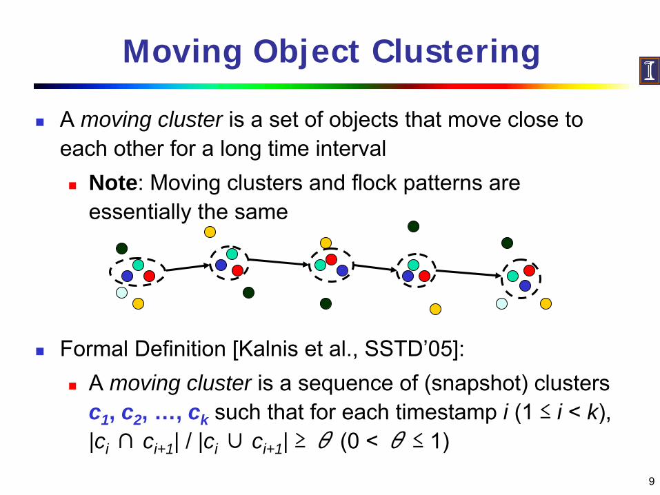
Moving Object Clustering
A moving cluster is a set of objects that move close to each other for a long time interval
Note: Moving clusters and flock patterns are essentially the same
Formal Definition [Kalnis et al., SSTD’05]:A moving cluster is a sequence of (snapshot) clusters c1, c2, …, ck such that for each timestamp i (1 ≤ i < k), |ci ∩ ci+1| / |ci ∪ ci+1| ≥ θ (0 < θ ≤ 1)
10
Retrieval of Moving Clusters (Kalnis et al. SSTD’05)
Basic algorithm (MC1)
1. Perform DBSCAN for each time slice
2. For each pair of a cluster c and a moving cluster g, check if g can be extended by c
If yes, g is used at the next iteration
If no, g is returned as a result
Improvements
MC2: Avoid redundant checks (Improve Step 2)
MC3: Reduce the number of executing DBSCAN (Improve Step 1)

11
Relative Motion Patterns (Laube et al. 04, Gudmundsson et al. 07)
Flock (m > 1, r > 0): At least m entities are within a circular region of radius r and they move in the same directionLeadership (m > 1, r > 0, s > 0) At least m entities are within a circular region of radius r, they move in the same direction, and at least one of the entities was already heading in this direction for at least s time stepsConvergence (m > 1, r > 0) At least m entities will pass through the same circular region of radius r (assuming they keep their direction)Encounter (m > 1, r > 0) At least m entities will be simultaneously inside the same circular region of radius r (assuming they keep their speed and direction)
12
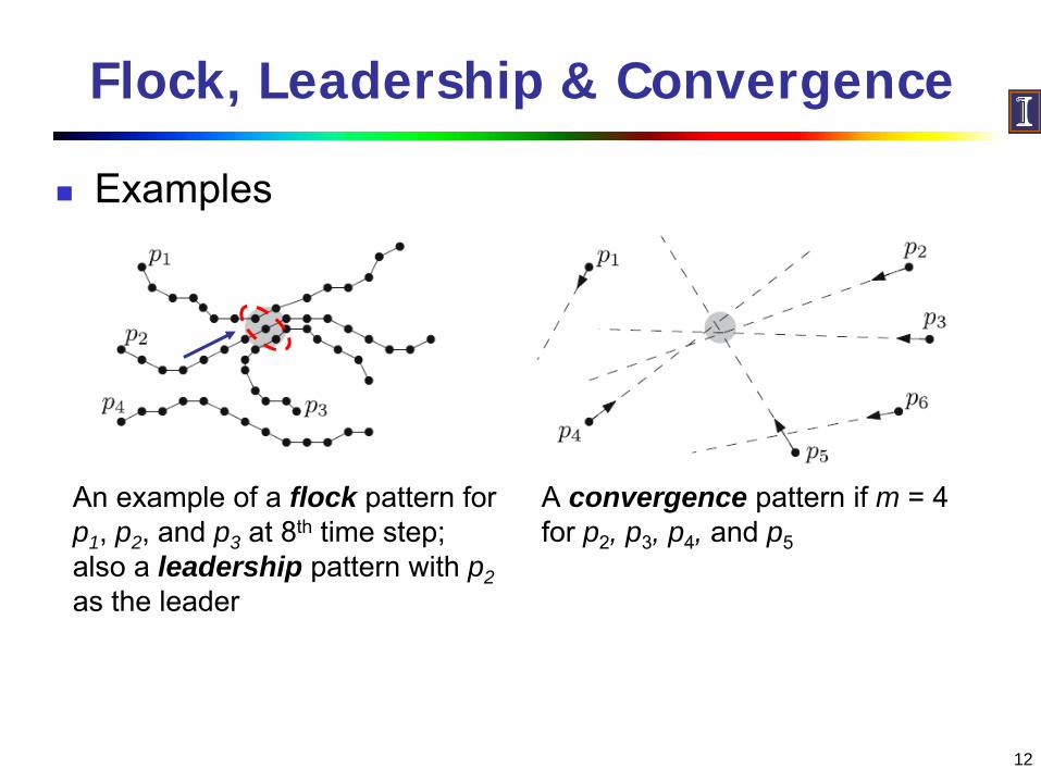
Flock, Leadership & Convergence
Examples
An example of a flock pattern for p1 , p2 , and p3 at 8th
time step; also a leadership pattern with p2 as the leader
A convergence pattern if m = 4 for p2
, p3
, p4
, and p5
13
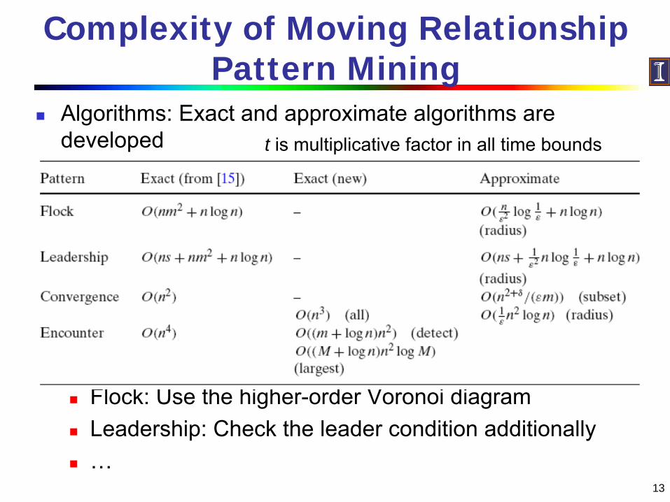
Complexity of Moving Relationship Pattern Mining
Algorithms: Exact and approximate algorithms are developed
Flock: Use the higher-order Voronoi diagramLeadership: Check the leader condition additionally…
t is multiplicative factor in all time bounds

14
An Extension of Flock Patterns (Gudmundsson et al. GIS’06, Benkert et al. SAC’07)
A new definition considers multiple time steps, whereas the previous definition only one time stepFlock: A flock in a time interval I, where the duration of Iis at least k, consists of at least m entities such that for every point in time within I, there is a disk of radius r that contains all the m entities
e.g.,
A flock through 3 time steps
15
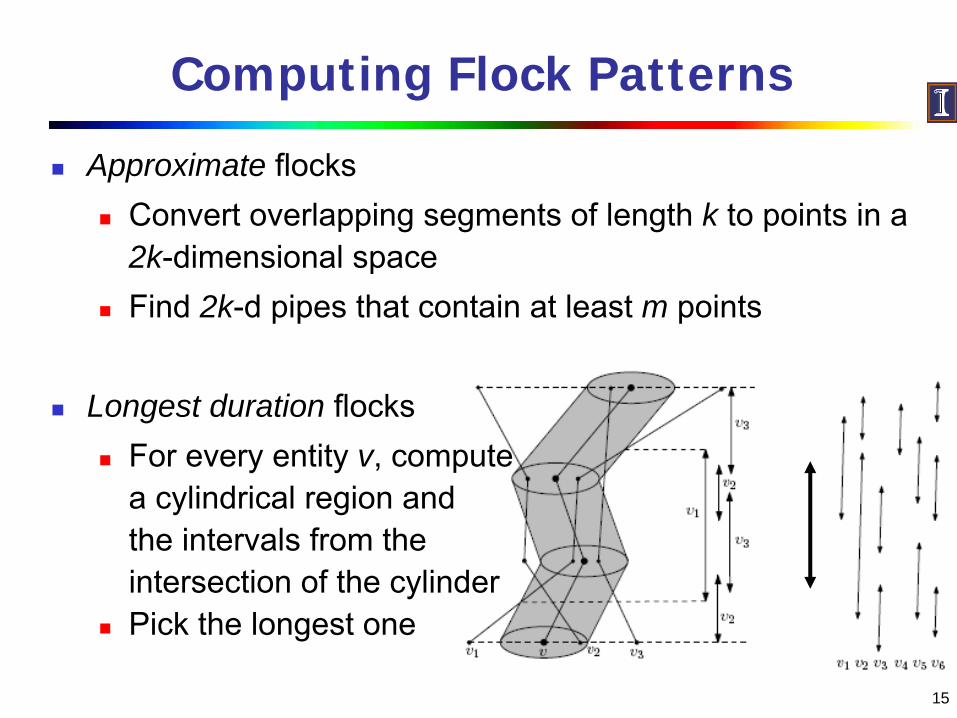
Computing Flock Patterns
Approximate flocksConvert overlapping segments of length k to points in a 2k-dimensional spaceFind 2k-d pipes that contain at least m points
Longest duration flocksFor every entity v, compute a cylindrical region andthe intervals from the intersection of the cylinderPick the longest one

Convoy: An Extension of Flock Pattern (Jeung et al. ICDE’08 & VLDB’08)
16
Flock pattern has rigid definition with a circleConvoy use density-based clustering at each timestamp

Efficient Discovery of Convoys
Base-line algorithm:Calculate density-based clusters for each timestampOverlap clusters for every k consecutive timestamps
Speedup algorithm using trajectory simplificationTrajectory simplification
17

A Filter-and-Refine Framework for Convoy Mining
Filter-and-refine frameworkFilter: partition time intoλ-size time slot; a trajectory is transformed into a set of segments; density-based clustering on segments.Refine: Look into everyλ-size time slot, refine the clusters based on points.
18

19
An Extension of Leadership Patterns (Andersson et al. GeoInformatica 07)
Leadership: if there is an entity that is a leader of at least m entities for at least k time units
An entity ej is said to be a leader at time [tx, ty] for time-points tx, ty, if and only if ej does not follow anyone at time [tx, ty], and ej is followed by sufficiently many entities at time [tx, ty]
ei follows ej
||di
– dj
|| ≤
β
ei ej

20
Reporting Leadership Patterns
Algorithm: Build and use the follow-arrays
e.g., Store nonnegative integers specifying for how many past consecutive unit-time-intervals ej is following ei (ej ≠
ei )

Swarms: A Relaxed but Real, Relative Movement Pattern
Flock and convoy all require k consecutive time stamps (still very rigid definition)Moving objects may not be close to each other for consecutive time stamps (need to relax time constraint)
21

Discovery of Swarm Patterns
A system that mines moving object patterns: Z. Li, et al., “MoveMine: Mining Moving Object Databases", SIGMOD’10 (system demo)
Z. Li, B. Ding, J. Han, and R. Kays, “Swarm: Mining Relaxed Temporal Moving Object Clusters”, in submission
← Convoy
discovers
only restricted patterns
Swarm
discovers
more patterns →
23
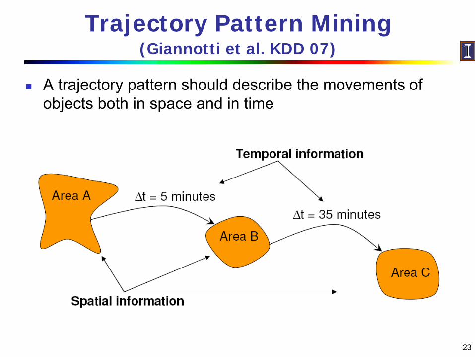
Trajectory Pattern Mining (Giannotti et al. KDD 07)
A trajectory pattern should describe the movements of objects both in space and in time
24
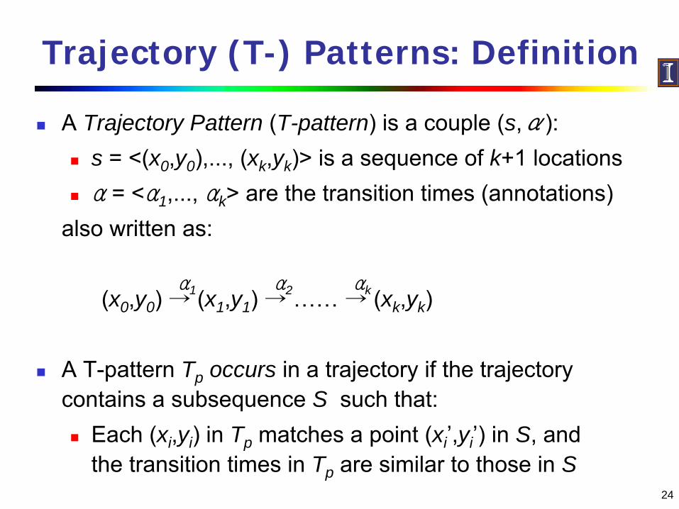
Trajectory (T-) Patterns: Definition
A Trajectory Pattern (T-pattern) is a couple (s,α):s = <(x0,y0),..., (xk,yk)> is a sequence of k+1 locationsα = <α1,..., αk> are the transition times (annotations)
also written as:
(x0 ,y0 ) → (x1 ,y1 ) →……→ (xk ,yk )
A T-pattern Tp occurs in a trajectory if the trajectory contains a subsequence S such that:
Each (xi,yi) in Tp matches a point (xi’,yi’) in S, and the transition times in Tp are similar to those in S
α1 α2 αk

25
Characteristics of Trajectory-Patterns
Routes between two consecutive regions are not relevant
Absolute times are not relevant
A B
These two movements are not discriminated
1 hour
1 hour
A B
These two movements are not discriminated
1 hour at 5 p.m.
1 hour at 9 a.m.
26
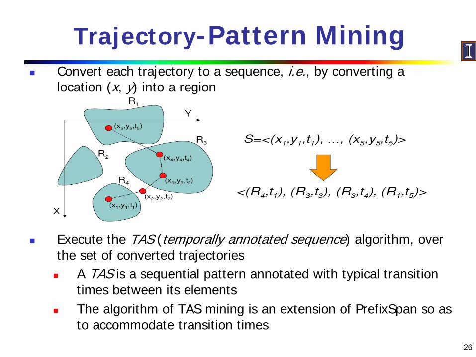
Trajectory-Pattern MiningConvert each trajectory to a sequence, i.e., by converting a location (x, y) into a region
Execute the TAS (temporally annotated sequence) algorithm, over the set of converted trajectories
A TAS is a sequential pattern annotated with typical transition times between its elementsThe algorithm of TAS mining is an extension of PrefixSpan so as to accommodate transition times

27
Sample Trajectory-Patterns
Data Source: Trucks in Athens – 273 trajectories)

28
Part I. Moving Object Data Mining
Introduction
Movement Pattern Mining
Periodic Pattern Mining
Clustering
Prediction
Classification
Outlier Detection

29
Spatiotemporal Periodic Pattern (Mamoulis et al. KDD 04)
In many applications, objects follow the same routes (approximately) over regular time intervals
e.g., Bob wakes up at the same time and then follows, more or less, the same route to his work everyday
Day 1:Day 2:Day 3:

30
Period and Periodic Pattern
Let S be a sequence of n spatial locations, {l0, l1, …, ln-1},
representing the movement of an object over a long
history
Let T << n be an integer called period, and T is given
A periodic pattern P is defined by a sequence r0r1…rT-1 of
length T that appears in S by more than min_sup times
For every ri in P, ri = * or lj*T+i is inside ri
31
Periodic Pattern Mining (I)
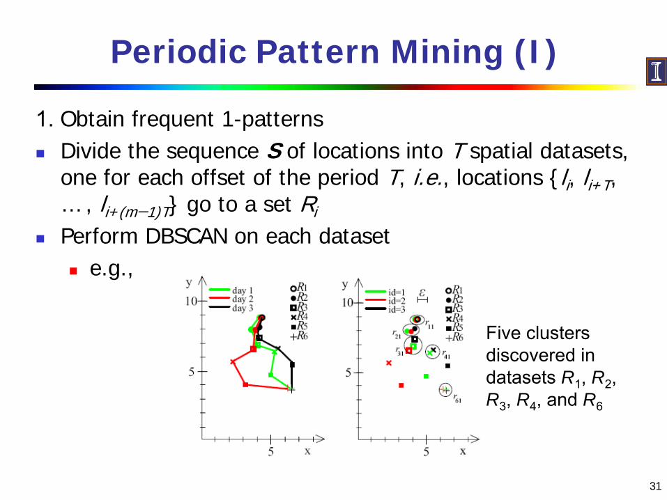
1. Obtain frequent 1-patternsDivide the sequence S of locations into T spatial datasets, one for each offset of the period T, i.e., locations {li, li+T, … , li+(m−1)T} go to a set Ri
Perform DBSCAN on each datasete.g.,
Five clusters discovered in datasets R1
, R2
, R3
, R4
, and R6

32
Periodic Pattern Mining (II)
2. Find longer patterns: Two methodsBottom-up level-wise technique
Generate k-patterns using a pair of (k-1)-patterns with their first k−2 non-* regions in the same positionUse a variant of the Apriori-TID algorithm
r1wr1x
r2y
r3z
r1ar1d
r2br2e
r3c
r3fr1a r2b r3cr1d r2e r3f
2-length patterns generated 3-length patterns

33
Periodic Pattern Mining (III)
Faster top-down approachReplace each location in S with the cluster-id which it belongs to or with * if the location belongs to no clusterUse the sequence mining algorithm to discover fast all frequent patterns of the form r0r1…rT−1, where each ri is a cluster in a set Ri or *Create a max-subpattern tree and traverse the tree in a top-down, breadth-first order
Periodic Patterns of Moving objects
Periodic behavior is the intrinsic behavior for most moving objectsYearly migration of birds
Fly to south for winter, fly back to north for summerPeople’s daily routines
Go to office at 9:00am, back home around 6:00pmDetecting periodic behavior is useful for:
Summarizing over long historical movementPeople’s behavior could be summarized as some daily behavior and weekly behavior
Predicting future movementE.g., predict the location at the future time (next day, next week, or next year)
Help detect abnormal eventsA bird does not follow its usual migration path ⇒ a signal of environment change
34

Challenges of Periodic Pattern Mining
35
interleaved periodsinterleaved periods
multiple periodsmultiple periods different locationsdifferent locations

Detection of Periods: A Naïve Method
Transform the movement points into complex plane (x, y) → x-yi(x, y) → y-xi
Apply Fourier Transform Weakness:
Affected by noise(x, y) → x-yi and y-xi, each produce different resultIt cannot detect partial period
Short FFT solves partial period problem, but it is not easy to generalize the result
36

A Motivating Example: Trajectories of Bees
Bee and Flower:8 hours stays in the nest16 hours fly nearby
37

FFT Transformation Does Not Work
38
(x,y) => x‐yi (x,y) => y‐xi
FFT should have strongest power at 42.7
(T = 24, NFFT/T = 1024/24 = 42.7)Failed!
Transform (x,y) into complex plane (two ways to transform)
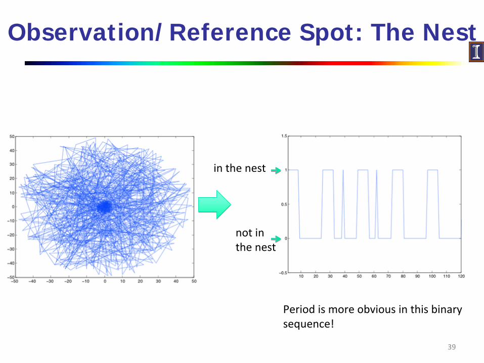
Observation/Reference Spot: The Nest
39
not in
the nest
in the nest
Period is more obvious in this binary
sequence!

Algorithm General Framework
Detecting periods: Use observation spots to find multiple interleaved periods
Observation spots are detected using density-based methodPeriods are detected for each obs. spot using Fourier Transform and auto-correlation
Summarizing periodic behaviors: via clusteringGive the statistical explanation of the behaviorE.g., “David has 80% probability to be at the office.”
40

Running Example: Bald Eager Migration
41Real data of a bald eagle over 3 years

Method: Finding Observation Spots
Observation spots:Frequently visited regions/locationsThey should have higher density than a random location
Partition the map into grids and use kernel-based method to find high density regions:
Find the observation spots using the contour of high density places
42

Example: Finding Observation Spots
43
Density Observation spots

Period Detection for Each Observation Spot
For each observation spot, the movement is transformed into a binary sequence.
0: not in the obs. spot
1: in the obs. spot
Use Fourier Transform combined with auto-correlation to find the periods
44

Example: Detect Periods for Each Obs. Spot
45
Period candidates first
detected using Fourier
Transform
The exact period is
further refined using
circular autocorrelation
Summarizing Periodic Behaviors
For each period, the movement is divided into segmentsif the period is “day”, each segment is a day
Some segments during a time period form a periodic behavior
Daily behavior in summerDaily behavior in winter
To distinguish interleaved behavior, apply clustering on the segmentsA representative behavior is summarized over all the segments in a cluster
46

Example: Summarizing Periodic Behaviors
47
Jan.‐Mar.Apr.‐June July‐.Oct Nov. Dec.

48
Part I. Moving Object Data Mining
Introduction
Movement Pattern Mining
Periodic Pattern Mining
Clustering
Prediction
Classification
Outlier Detection
Clustering: Distance-Based vs. Shape-Based
Distance-based clustering: Find a group of objects moving together For whole time span
high-dimensional clusteringprobabilistic clustering
For partial continuous time spandensity-based clusteringmoving cluster, flock, convoy (borderline case between clustering and patterns)
For partial discrete time spanswarm (borderline case between clustering and patterns)
Shape-based clustering: Find similar shape trajectoriesVariants of shape: translation, rotation, scaling, and transformationSub-trajectory clustering
49

High-Dimensional Clustering & Distance Measures
Treat each timestamp as one dimension
Many high-dimensional clustering methods can be applied to cluster moving objects
Most popular high-dimensional distance measure
Euclidean distance
Dynamic Time Warping
Longest Common Subsequence
Edit Distance with Real Penalty
Edit Distance on Real Sequence
50

High-Dimensional Distance Measures
Distance Measure Local Time Shifting
Noise Metric Complexity
Euclidean ✔ O(n)DTW (Yi et al., ICDE’98) ✔ O(n2)
LCSS (Vlachos et al., KDD’03) ✔ ✔ O(n2)
ERP (Chen et al., VLDB’04) ✔ ✔ O(n2)
EDR (Chen et al., SIGMOD’05) ✔ ✔(consider gap)
O(n2)
51
52
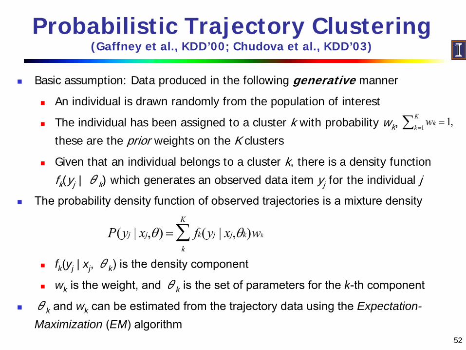
Probabilistic Trajectory Clustering (Gaffney et al., KDD’00; Chudova et al., KDD’03)
Basic assumption: Data produced in the following generative manner
An individual is drawn randomly from the population of interest
The individual has been assigned to a cluster k with probability wk,
these are the prior weights on the K clusters
Given that an individual belongs to a cluster k, there is a density function
fk(yj | θk) which generates an observed data item yj for the individual j
The probability density function of observed trajectories is a mixture density
fk(yj | xj, θk) is the density component
wk is the weight, and θk is the set of parameters for the k-th component
θk and wk can be estimated from the trajectory data using the Expectation-Maximization (EM) algorithm
∑ ==
K
kkw
1,1
P(yj | xj,θ) = fk(yj | xj,θk)wk
k
K
∑

53Tracks Atlantic named Tropical Cyclones 1970-2003.
TRACKS
Mean RegressionTrajectory
Clustering Results For Hurricanes (Camargo et al. 06)
54
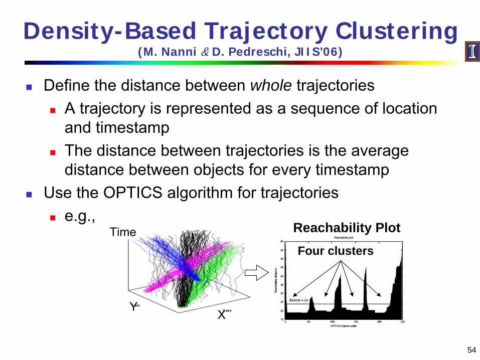
Density-Based Trajectory Clustering (M. Nanni & D. Pedreschi, JIIS’06)
Define the distance between whole trajectoriesA trajectory is represented as a sequence of location and timestampThe distance between trajectories is the average distance between objects for every timestamp
Use the OPTICS algorithm for trajectoriese.g.,
XY
TimeFour clusters
Reachability Plot
55
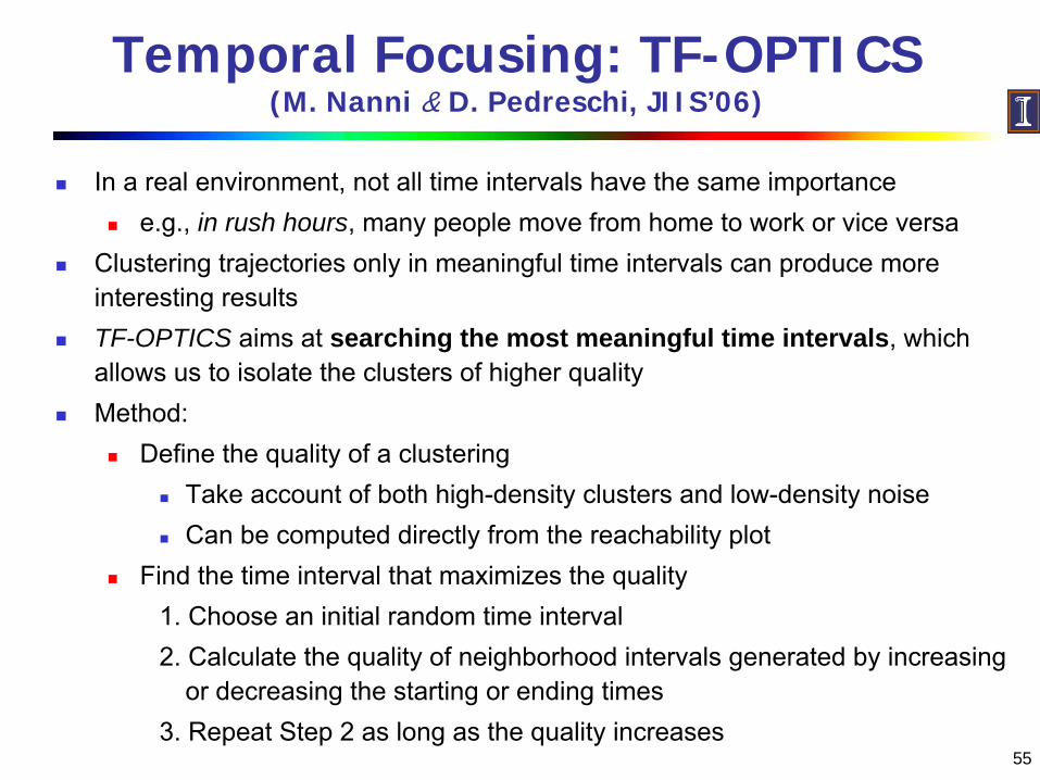
Temporal Focusing: TF-OPTICS (M. Nanni & D. Pedreschi, JIIS’06)
In a real environment, not all time intervals have the same importancee.g., in rush hours, many people move from home to work or vice versa
Clustering trajectories only in meaningful time intervals can produce more interesting resultsTF-OPTICS aims at searching the most meaningful time intervals, which allows us to isolate the clusters of higher qualityMethod:
Define the quality of a clusteringTake account of both high-density clusters and low-density noiseCan be computed directly from the reachability plot
Find the time interval that maximizes the quality1. Choose an initial random time interval2. Calculate the quality of neighborhood intervals generated by increasing
or decreasing the starting or ending times3. Repeat Step 2 as long as the quality increases

Invariant Distance Measures for Trajectories (Vlachos et al., KDD’04)
Invariants: Translation, Rotation, Scaling, Transformation
Map each trajectory to a trajectory in a rotation invariant space.Movement vector: angles of each movement vector is relative to a reference vectorAngle/Arc-Length pairs (AAL)
Use Dynamic Time Warping (DTW) to measure the distance in invariant space
56
Similar trajectories in different invariants

57
Trajectory Clustering: A Partition-and- Group Framework (Lee et al., SIGMOD’07)
Existing algorithms group trajectories as a whole ⇒ They might not be able to find similar portions of trajectories
e.g., common behavior cannot be discovered since TR1~TR5 move to totally different directions
Partition-and-group: discovers common sub-trajectories
Usage: Discover regions of special interestHurricane Landfall Forecasts: Discovery of common behaviors of hurricanes near the coastline or at sea (i.e., before landing)
Effects of Roads and Traffic on Animal Movements: Discover common behaviors of animals near the road
A common sub-trajectoryTR2
TR3TR5
TR1
TR4

58
Partition-and-Group: Overall Procedure
Two phases: partitioning and groupingTR5
TR1
TR2
TR3TR4
A set of trajectories
A set of line segmentsA cluster
(1) Partition
(2) Group
A representative trajectory
Note: A representative trajectory is a common sub-trajectory
59
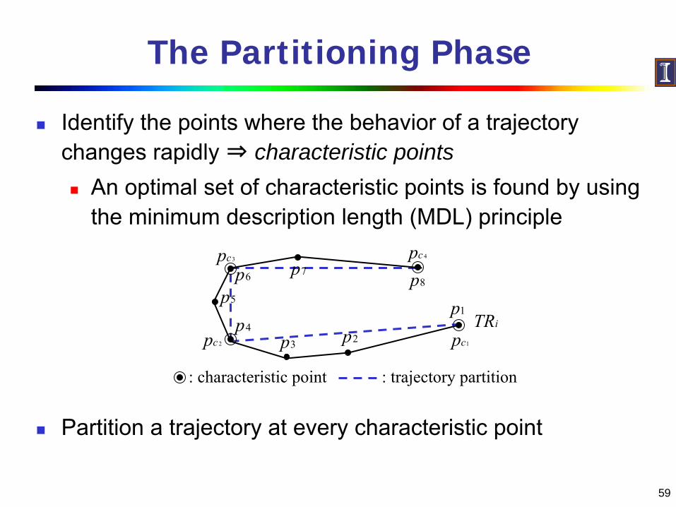
The Partitioning Phase
Identify the points where the behavior of a trajectory changes rapidly ⇒ characteristic points
An optimal set of characteristic points is found by using the minimum description length (MDL) principle
Partition a trajectory at every characteristic point
1p2p3p
4p5p
6p 7p8p
: characteristic point : trajectory partition
1cp2cp
3cp 4cp
iTR

60
Overview of the MDL Principle
The MDL principle has been widely used in information theory
The MDL cost consists of two components: L(H) and L(D|H), where H means the hypothesis, and D the data
L(H) is the length, in bits, of the description of the hypothesis
L(D|H) is the length, in bits, of the description of the data when encoded with the help of the hypothesis
The best hypothesis H to explain D is the one that minimizes the sum of L(H) and L(D|H)

61
MDL Formulation
Finding the optimal partitioning translates to finding the best hypothesis using the MDL principle
H → a set of trajectory partitions, D → a trajectoryL(H) → the sum of the length of all trajectory partitionsL(D|H) → the sum of the difference between a trajectory and a set of its trajectory partitions
L(H) measures conciseness; L(D|H) preciseness
)),(),(),((log)),(),(),((log)|(
))((log)(
4341324121412
4341324121412
412
ppppdppppdppppdppppdppppdppppdHDL
pplenHL
θθθ +++++=
=⊥⊥⊥
1cp 2cp1p
2p 3p
4p
5p

62
Grouping Phase (1/2)
Find the clusters of trajectory partitions using density-based clustering (i.e., DBSCAN)
A density-connect component forms a cluster, e.g., { L1, L2, L3, L4, L5, L6 }
L1L3
L5 L2 L4
L6
L6 L5
L3
L1
L2
L4
MinLns
= 3

63
Grouping Phase (2/2)
Describe the overall movement of the trajectory partitions that belong to the cluster
A red line: a representative trajectory, A blue line: an average direction vector,
Pink lines: line segments in a density-connected set

64
Example: Trajectory Clustering Results
570 Hurricanes (1950~2004)
Seven clusters discovered from the hurricane data set
Red line: a representative trajectory
Two clusters discovered from a deer data set
65
Part I. Moving Object Data Mining
Introduction
Movement Pattern Mining
Periodic Pattern Mining
Clustering
Prediction
Classification
Outlier Detection
Location Prediction for Moving Objects
Predicting future location
Based on its own history of one moving object
Linear (not practical) vs. non-linear motion (more practical)
Vector based (predict near time, e.g., next minute) vs. pattern based (predict distant time, e.g., next month/year)
Based on all moving objects’ trajectories
based on frequent patterns
66
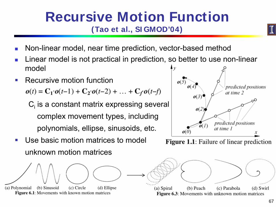
Recursive Motion Function (Tao et al., SIGMOD’04)
Non-linear model, near time prediction, vector-based methodLinear model is not practical in prediction, so better to use non-linear model
67
Recursive motion function
Ci
is a constant matrix expressing several complex movement types, including polynomials, ellipse, sinusoids, etc.
Use basic motion matrices to model unknown motion matrices

Efficient Implementation: Recursive Motion Prediction
Indexing expected trajectories using Spatio-Temporal Prediction Tree (STP-Tree)A combination of Time Parameterized R Tree (TPR-tree) and TPR*-tree
68

Experimental Results: Recursive Motion Prediction
Effectiveness (wrt retrospect)
Efficiency using STP-tree indexing
69

Hybrid Prediction (Jeung et al. , ICDE’08)
Combining pattern and vector to prediction locations
Can predict both distant and near time locations
Mining frequent periodic patterns
70
Ex: inadequate prediction using vector-based method
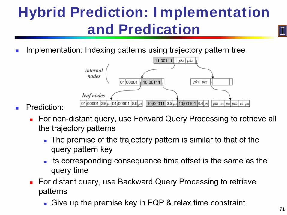
Hybrid Prediction: Implementation and Predication
Implementation: Indexing patterns using trajectory pattern tree
Prediction:For non-distant query, use Forward Query Processing to retrieve all the trajectory patterns
The premise of the trajectory pattern is similar to that of the query pattern keyits corresponding consequence time offset is the same as the query time
For distant query, use Backward Query Processing to retrieve patterns
Give up the premise key in FQP & relax time constraint71

Prediction Using Frequent Trajectory Patterns (Monreale et al., KDD’09)
Use frequent T-patterns of other moving objectsIf many moving objects follow a pattern, it is likely that a moving object will also follow this patternMethod
Mine T-PatternsConstruct T-Pattern TreePredict using T-pattern tree
72
T-Patterns
73
Part I. Moving Object Data Mining
Introduction
Movement Pattern Mining
Periodic Pattern Mining
Clustering
Prediction
Classification
Outlier Detection

74
Trajectory Classification
Task: Predict the class labels of moving objects based on their trajectories and other features
Two approaches
Machine learning techniques
Studied mostly in pattern recognition, bioengineering, and video surveillance
The hidden Markov model (HMM)
Trajectory-based classification (TraClass): Trajectory classification using hierarchical region-based and trajectory-based clustering

75
Machine Learning for Trajectory Classification (Sbalzarini et al. 02)
Compare various machine learning techniques for biological trajectory classificationData encoding
For the hidden Markov model, a whole trajectory is encoded to a sequence of the momentary speedFor other techniques, a whole trajectory is encoded to the mean and the minimum of the speed of a trajectory, thus a vector in R2
Two 3-class datasets: Trajectories of living cells taken from the scales of the fish Gillichthys mirabilis
Temperature dataset: 10°C, 20°C, and 30°CAcclimation dataset: Three different fish populations

76
Machine Learning Techniques Used
k-nearest neighbors (KNN)A previously unseen pattern x is simply assigned to the same class to which the majority of its k-nearest neighbors belongs
Gaussian mixtures with expectation maximization (GMM)Support vector machines (SVM)Hidden Markov models (HMM)
Training: Determine the model parameters λ = (A, B, π) to maximize P [x | λ] for a given observation x
Temperature data set
Acclimation data set
Evaluation: Given an observation x = { O1, …, OT } and a model λ= (A, B, π), compute the probability P [x | λ] that the observation xhas been produced by a source described by λ

77
Vehicle Trajectory Classification (Fraile and Maybank 98)
The measurement sequence is divided into overlapping
segments
In each segment, the trajectory of the car is approximated
by a smooth function and then assigned to one of four
categories: ahead, left, right, or stop
The list of segments is reduced to a string of symbols
drawn from the set {a, l, r, s}
The string of symbols is classified using the hidden
Markov model (HMM)

78
Use of the HMM for Classification
Classification of the global motions of a car is carried out using an HMM
The HMM contains four states which are in order A, L, R, S, which are the true states of the car: ahead, turning left, turning right, stopped
The HMM has four output symbols in order a, l, r, s, which are the symbols obtained from the measurement segments
The Viterbi algorithm is used to obtain the sequence of internal states
Observed symbols
Sequence of inferred states
This measurement sequence means the driver stops and then turns to the right
Measurement sequence
79
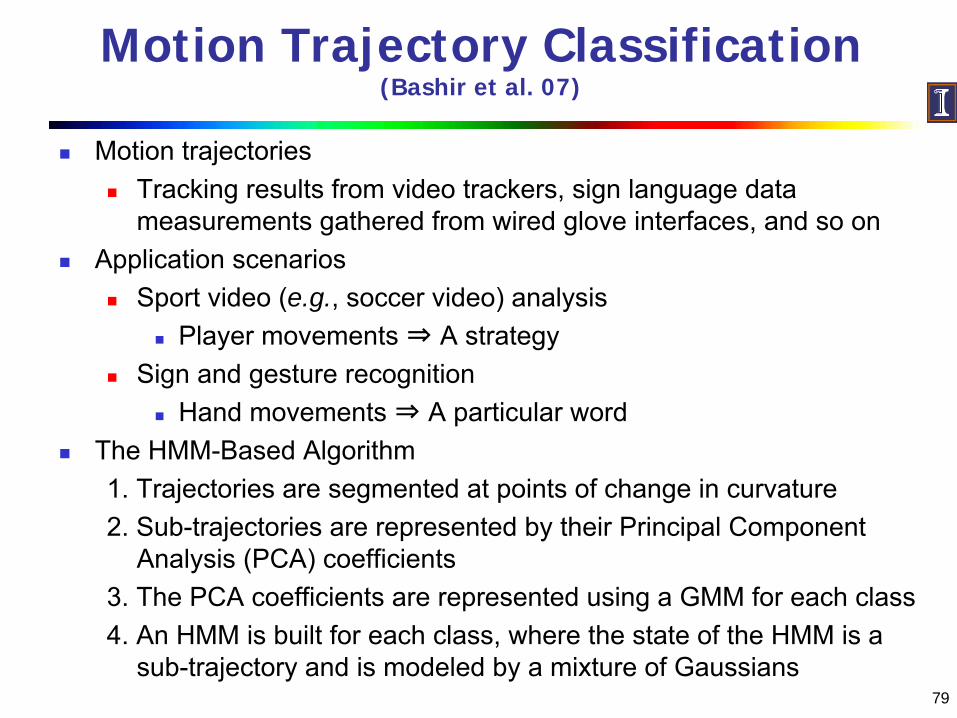
Motion Trajectory Classification (Bashir et al. 07)
Motion trajectoriesTracking results from video trackers, sign language data measurements gathered from wired glove interfaces, and so on
Application scenariosSport video (e.g., soccer video) analysis
Player movements ⇒ A strategySign and gesture recognition
Hand movements ⇒ A particular wordThe HMM-Based Algorithm1. Trajectories are segmented at points of change in curvature2. Sub-trajectories are represented by their Principal Component
Analysis (PCA) coefficients3. The PCA coefficients are represented using a GMM for each class4. An HMM is built for each class, where the state of the HMM is
a sub-trajectory and is modeled by a mixture of Gaussians
80
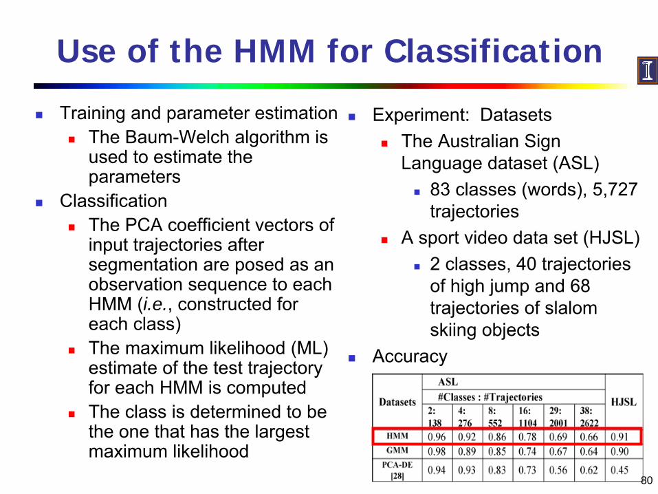
Use of the HMM for Classification
Training and parameter estimationThe Baum-Welch algorithm is used to estimate the parameters
ClassificationThe PCA coefficient vectors of input trajectories after segmentation are posed as an observation sequence to each HMM (i.e., constructed for each class)The maximum likelihood (ML) estimate of the test trajectory for each HMM is computedThe class is determined to be the one that has the largest maximum likelihood
Experiment: DatasetsThe Australian Sign Language dataset (ASL)
83 classes (words), 5,727 trajectories
A sport video data set (HJSL)2 classes, 40 trajectories of high jump and 68 trajectories of slalom skiing objects
Accuracy

81
A Critique of Previous Methods
Common Characteristics of Previous Methods: Use the shapes of whole trajectories to do classification
Encode a whole trajectory into a feature vector;
Convert a whole trajectory into a string or a sequence of the momentary speed; or
Model a whole trajectory using the HMM
Note: Although a few methods segment trajectories, the main purpose is to approximate or smooth trajectories before using the HMM
82
TraClass: Trajectory Classification Based on Clustering
Motivation
Discriminative features are likely to appear at parts of trajectories, not at whole trajectories
Discriminative features appear not only as common movement patterns, but also as regions
Solution
Extract features in a top-down fashion, first by region-based clustering and then by trajectory-based clustering

83
Intuition and Working Example
Parts of trajectories near the container port and near the refinery enable us to distinguish between container ships and tankers even if they share common long pathsThose in the fishery enable us to recognize fishing boats even if they have no common path there
Refinery
Fishery
Port A Port B
Container Port
Container Ships Tankers Fishing Boats
84
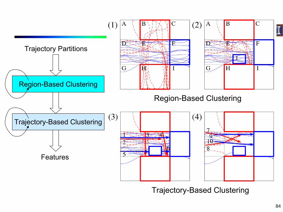
Region-Based Clustering
Trajectory-Based Clustering
Region-Based Clustering
Trajectory-Based Clustering
Trajectory Partitions
Features
85
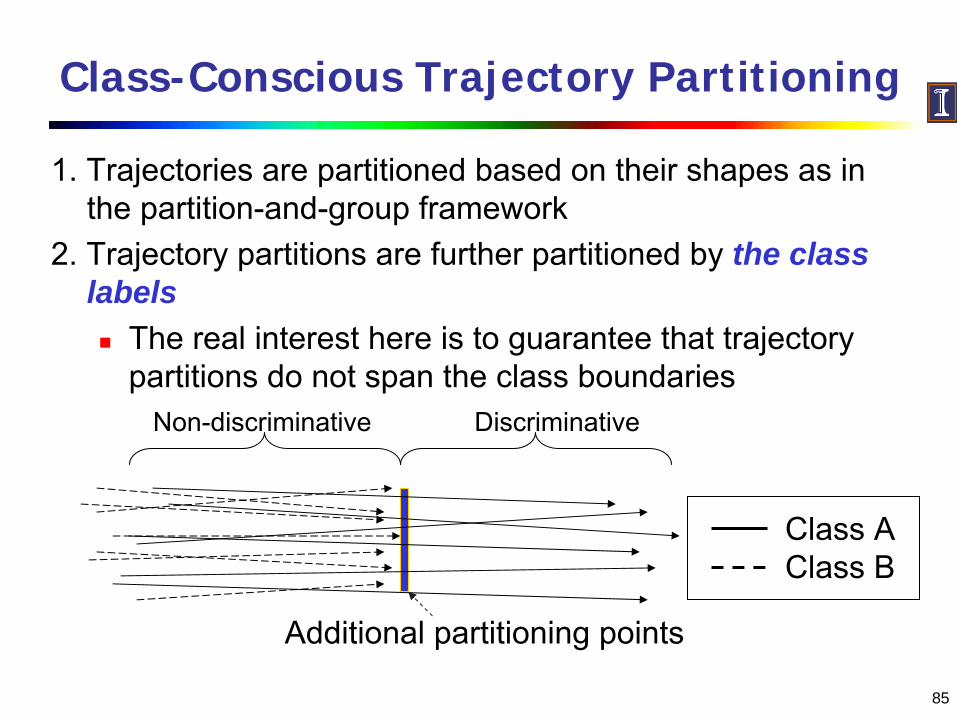
Class-Conscious Trajectory Partitioning
1. Trajectories are partitioned based on their shapes as in the partition-and-group framework
2. Trajectory partitions are further partitioned by the class labels
The real interest here is to guarantee that trajectory partitions do not span the class boundaries
Additional partitioning points
Non-discriminative Discriminative
Class AClass B

86
Region-Based Clustering
Objective: Discover regions that have trajectories mostly of one class regardless of their movement patternsAlgorithm: Find a better partitioning alternately for the X and Y axes as long as the MDL cost decreases
The MDL cost is formulated to achieve both homogeneity and conciseness
87
Trajectory-Based Clustering
Objective: Discover sub-trajectories that indicate common movement patterns of each class
Algorithm: Extend the partition-and-group framework for classification purposes so that the class labels are incorporated into trajectory clustering
If an ε-neighborhood contains trajectory partitions mostly of the same class, it is used for clustering; otherwise, it is discarded immediately
88
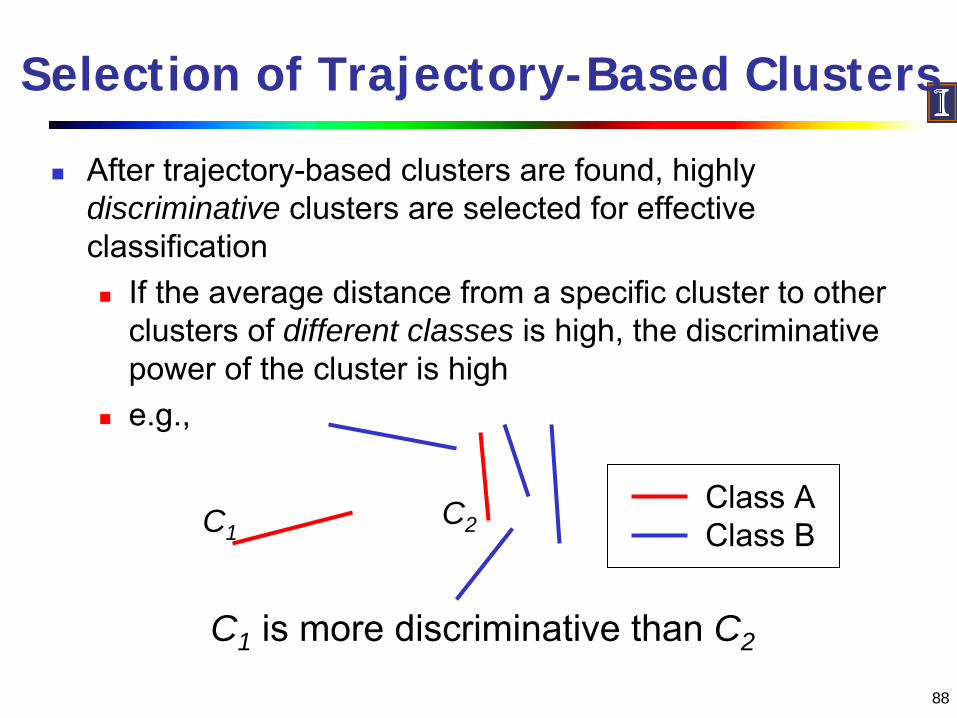
Selection of Trajectory-Based Clusters
After trajectory-based clusters are found, highly discriminative clusters are selected for effective classification
If the average distance from a specific cluster to other clusters of different classes is high, the discriminative power of the cluster is highe.g.,
C1C2
Class AClass B
C1 is more discriminative than C2
89
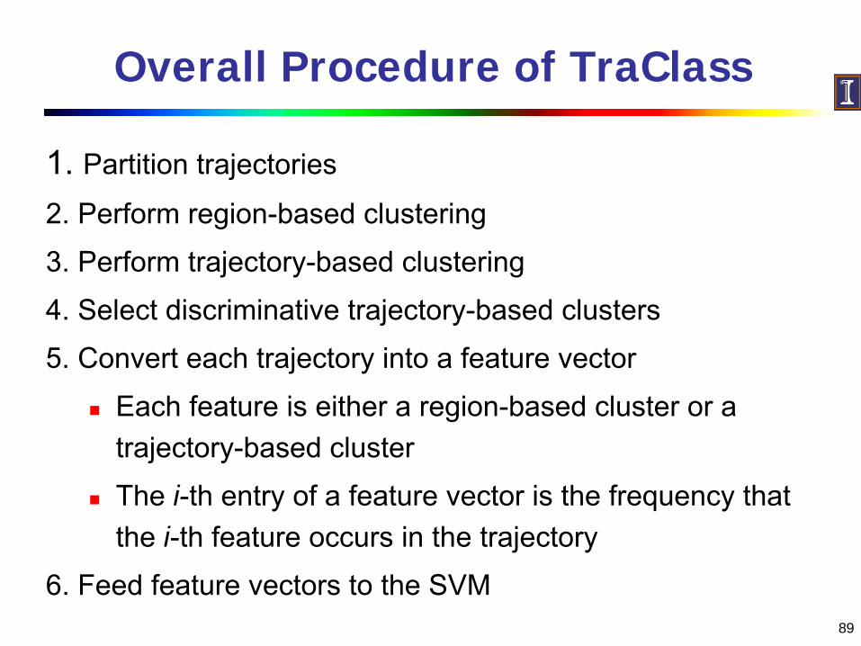
Overall Procedure of TraClass
1. Partition trajectories
2. Perform region-based clustering
3. Perform trajectory-based clustering
4. Select discriminative trajectory-based clusters
5. Convert each trajectory into a feature vector
Each feature is either a region-based cluster or a trajectory-based cluster
The i-th entry of a feature vector is the frequency that the i-th feature occurs in the trajectory
6. Feed feature vectors to the SVM

90
Classification Results
DatasetsAnimal: Three classes ← three species: elk, deer, and cattleVessel: Two classes ← two vesselsHurricane: Two classes ← category 2 and 3 hurricanes
MethodsTB-ONLY: Perform trajectory-based clustering onlyRB-TB: Perform both types of clustering
Results

91
Data (Three Classes)
Features:10 Region-Based Clusters37 Trajectory-Based Clusters
Accuracy = 83.3%
Example: Extracted Features

92
Part I. Moving Object Data Mining
Introduction
Movement Pattern Mining
Periodic Pattern Mining
Clustering
Prediction
Classification
Outlier Detection
93
Trajectory Outlier Detection
Task: Detect the trajectory outliers that are grossly different from or inconsistent with the remaining set of trajectories
Methods and philosophy:
1. Whole trajectory outlier detection
A unsupervised method
A supervised method based on classification
2. Integration with multi-dimensional information
3.
Partial trajectory outlier detection
A Partition-and-Detect framework

94
Outlier Detection: A Distance-Based Approach (Knorr et al. VLDBJ00)
Define the distance between two whole trajectoriesA whole trajectory is represented by
The distance between two whole trajectories is defined as
Apply a distance-based approach to detection of trajectory outliersAn object O in a dataset T is a DB(p, D)-outlier if at least fraction pof the objects in T lies greater than distance D from O
⎥⎥⎥⎥
⎦
⎤
⎢⎢⎢⎢
⎣
⎡
=
velocity
heading
end
start
PPPP
P
),,(),,(
),(),(
velocityvelocityvelocityvelocity
headingheadingheadingheading
endendend
startstartstart
minmaxavgPminmaxavgP
yxPyxP
====
[ ]velocityheadingendstart
velocity
heading
end
start
wwww
PPDPPD
PPDPPD
PPD ⋅
⎥⎥⎥⎥
⎦
⎤
⎢⎢⎢⎢
⎣
⎡
=
),(),(
),(),(
),(
21
21
21
21
21
where

95
Sample Trajectory Outliers
Detect outliers from person trajectories in a room
The entire data set The outliers only

96
Use of Neural Networks (Owens and Hunter 00)
A whole trajectory is encoded to a feature vector: F = [ x, y, s(x), s(y), s(dx), s(dy), s(|d2x|), s(|d2y|) ]
s() indicates a time smoothed average of the quantity
dx = xt – xt–1
d2x = xt – 2xt–1 + xt–2
A self-organizing feature map (SOFM) is trained using the feature vectors of training trajectories, and a new trajectory is classified into novel (i.e., suspicious) or not novel
Supervised learning
97
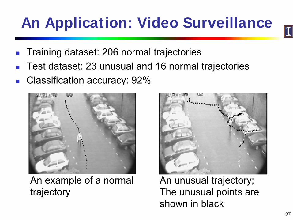
An Application: Video Surveillance
Training dataset: 206 normal trajectoriesTest dataset: 23 unusual and 16 normal trajectoriesClassification accuracy: 92%
An example of a normal trajectory
An unusual trajectory; The unusual points are shown in black

98
Anomaly Detection (Li et al. ISI’06, SSTD’07)
Automated alerts of abnormal moving objectsCurrent US Navy model: manual inspection
Started in the 1980s160,000 ships
99
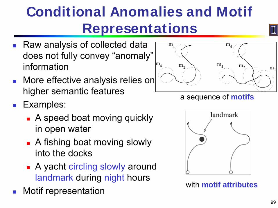
Conditional Anomalies and Motif Representations
Raw analysis of collected data does not fully convey “anomaly”informationMore effective analysis relies on higher semantic featuresExamples:
A speed boat moving quickly in open waterA fishing boat moving slowly into the docksA yacht circling slowly around landmark during night hours
Motif representation
a sequence of motifs
with motif attributes

100
Motif-Oriented Feature Space
Each motif expression has attributes (e.g., speed, location, size, time)Attributes express how a motif was expressed
A right-turn at 30mph near landmark Y at 5:30pmA straight-line at 120mph (!!!) in location X at 2:01am
Motif-Oriented Feature Space Naïve feature space
1. Map each distinct motif-expression to a feature2. Trajectories become feature vectors in the new space
Let there be A attributes attached to every motif, each trajectory is a set of motif-attribute tuples
{(mi , v1 ,
v2 , …, vA ), …, (mj , v1 , v2 , …, vA )}Example:
Object 1: {(right-turn, 53mph, 3:43pm)} → (1, 0)Object 2: {(right-turn, 50mph, 3:47pm)} → (0, 1)
101
Motif Feature Extraction
Intuition: Should have features that describe general high-level concepts
“Early Morning” instead of 2:03am, 2:04am, …
“Near Location X” instead of “50m west of Location X”
Solution: Hierarchical micro-clustering
For each motif attribute, cluster values to form higher level concepts
Hierarchy allows flexibility in describing objects
e.g., “afternoon” vs. “early afternoon” and “late afternoon”

102
Feature Clustering
Rough, fast micro-clustering
method based on BIRCH
(SIGMOD’96)
Extracts a hierarchy for every
motif-attribute combination
Trajectories can be
represented at arbitrary level
of granularity
103
Trajectory Outlier Detection: A Partition- and-Detect Framework (Lee et al. 08)
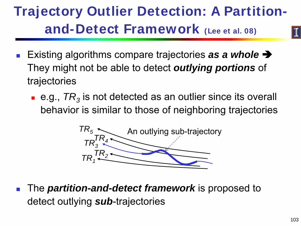
Existing algorithms compare trajectories as a wholeThey might not be able to detect outlying portions of trajectories
e.g., TR3 is not detected as an outlier since its overall behavior is similar to those of neighboring trajectories
The partition-and-detect framework is proposed to detect outlying sub-trajectories
TR5
TR1
TR4TR3TR2
An outlying sub-trajectory
104
Usefulness of Outlying Sub-Trajectories
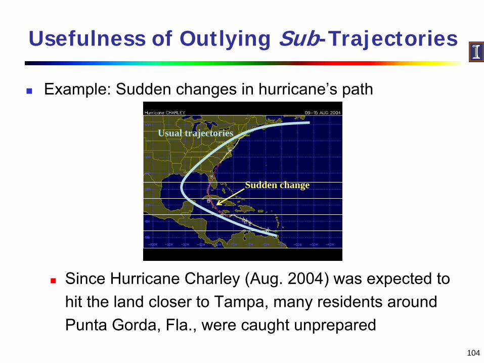
Example: Sudden changes in hurricane’s path
Since Hurricane Charley (Aug. 2004) was expected to hit the land closer to Tampa, many residents around Punta Gorda, Fla., were caught unprepared
Usual trajectories
Sudden change

105
Overall Procedure
Two phases: partitioning and detection
TR5
TR1
TR4TR3TR2
A set of trajectories
(1) Partition
(2) DetectTR3
A set of trajectory partitions
An outlier
Outlying trajectory partitions

106
Simple Trajectory Partitioning
A trajectory is partitioned at a base unit: the smallest meaningful unit of a trajectory in a given application
e.g., The base unit can be every single point
Pros: High detection quality in general
Cons: Poor performance due to a large number of t- partitions Propose a two-level partitioning strategy
Neighboring TrajectoriesA t-partition
A trajectory TRout
An outlying t-partition

107
Two-Level Trajectory Partitioning
Objective Achieves much higher performance than the simple strategyObtains the same result as that of the simple strategy; i.e., does not lose the quality of the result
Basic idea1. Partition a trajectory in coarse granularity first2. Partition a coarse t-partition in fine granularity only
when necessaryMain benefit
Narrows the search space that needs to be inspected in fine granularity ⇒ Many portions of trajectories can be pruned early on

108
Intuition of Two-Level Trajectory Partitioning
If the distance between coarse t-partitions is very large (or small), the distances between their fine t-partitions are also very large (or small)
The lower and upper bounds for fine t-partitions are derived in the paper
TRi
TRj
Coarse-Granularity Partitioning
Fine-Granularity Partitioning

109
Outlier Detection
Once trajectories are partitioned, trajectory outliers are detected based on both distance and density
An outlying t-partition is defined as
A trajectory is an outlier if it contains a sufficient amount of outlying t-partitions
iLiTR
Li is an outlying t-partition Li is not an outlying t-partition
Not close
≤ 1‒piLiTR
Close > 1‒p

110
Incorporation of Density
The number of close trajectories is adjusted by the density of a t-partition
Dense region Decreased, Sparse region Increased
T-Partitions in dense regions are favored!
111
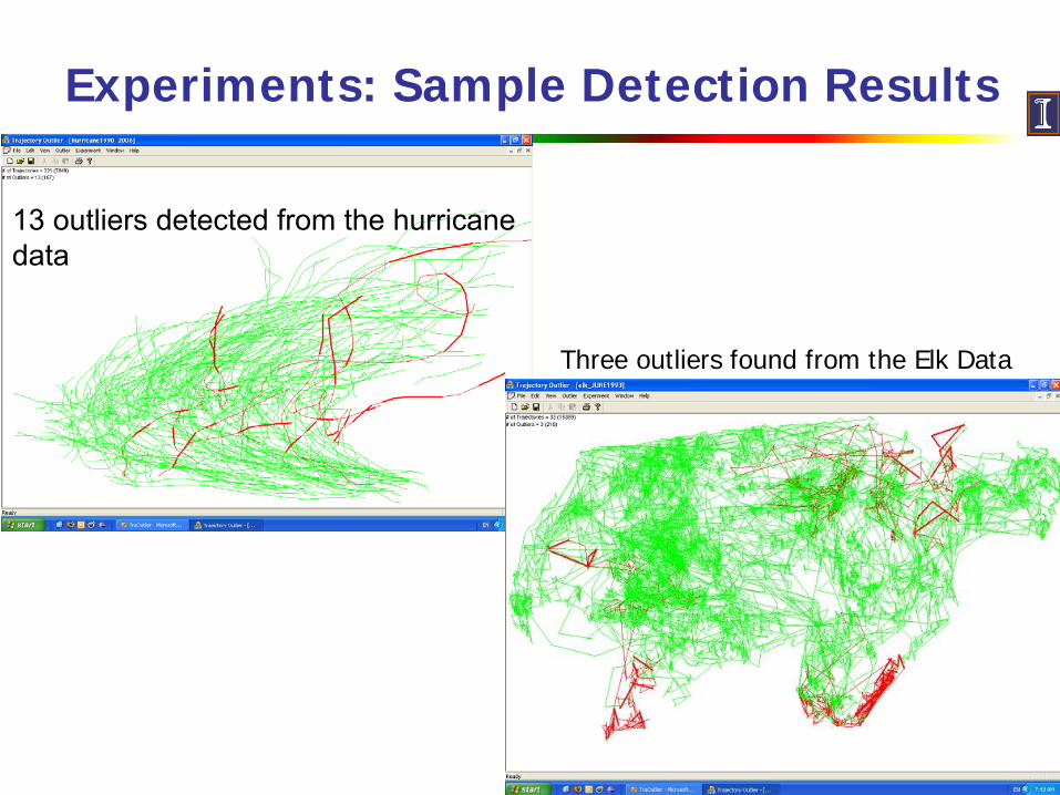
Experiments: Sample Detection Results
13 outliers detected from the hurricane data
Three outliers found from the Elk Data
112
Summary: Moving Object Mining
Pattern MiningTrajectory patterns, flock and leadership patterns, periodic patterns,
ClusteringProbabilistic method, density-based method, partition-and-group framework
Predictionlinear/non-linear model, vector-based method, pattern-based method
ClassificationMachine learning-based method, HMM-based method, TraClassusing collaborative clustering
Outlier DetectionUnsupervised method, supervised method, partition-and-detect framework

113
Tutorial Outline
Part I. Mining Moving Objects
Part II. Mining Traffic Data
Part III. Conclusions

114
Part II. Traffic Data Mining
Introduction to Traffic Data
Traffic Data Warehousing
Route Discovery by Frequent Path Pattern
Analysis

115
Trillion Miles of Travel
MapQuest
10 billion routes computed by 2006
GPS devices
18 million sold in 2006
88 million by 2010
Lots of driving
2.7 trillion miles of travel (US – 1999)
4 million miles of roads
$70 billion cost of congestion, 5.7 billion gallons of wasted gas

116
Abundant Traffic Data
Google Maps provides live traffic information

117
Traffic Data Gathering
Inductive loop detectorsThousands, placed every few miles in highways
Only aggregate data
CamerasLicense plate detection
RFIDToll booth transponders
511.org – readers in CA
118
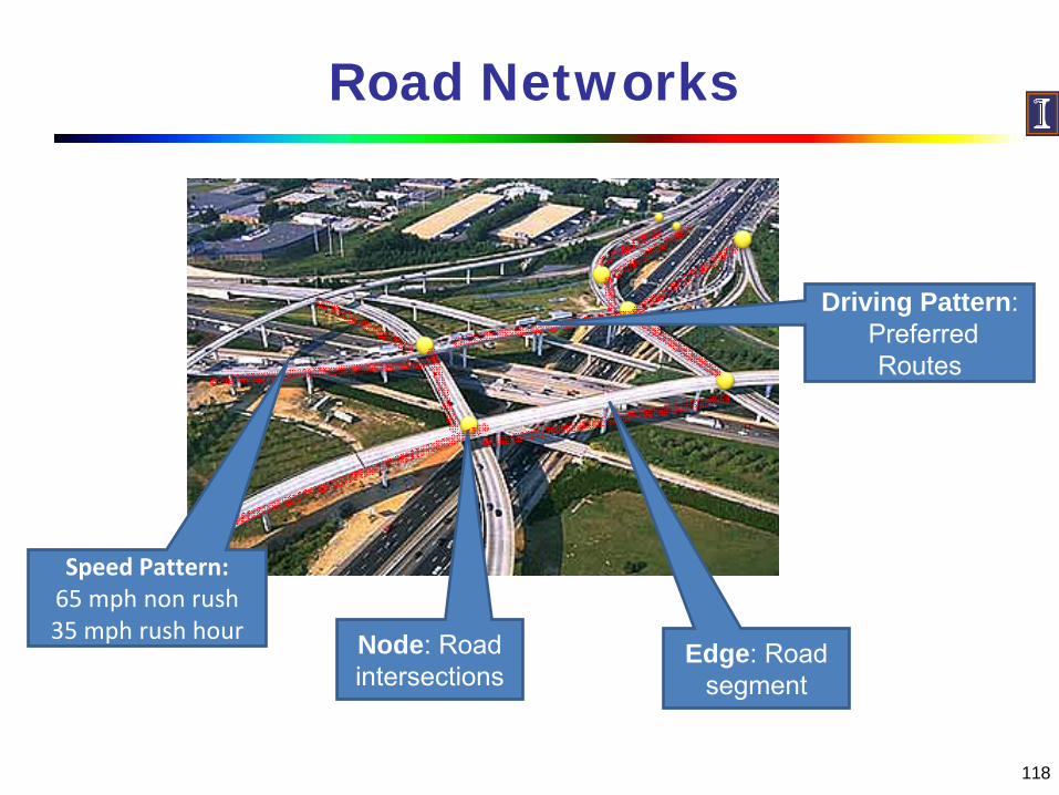
Road Networks
Node: Road intersections
Edge: Road segment
Driving Pattern:Preferred Routes
Speed Pattern:65 mph non rush35 mph rush hour

119
Part II. Traffic Data Mining
Introduction to Traffic Data
Traffic Data Warehousing
Route Discovery by Frequent Path Pattern
Analysis

Traffic Cube: Motivation Examples
Ex. 1. Bob is a bagpack traveler and he is new to Los Angles. He wants to know
Where are the places the traffic jams are most likely to happen in weekend?When is the best time to visit the Hollywood to avoid heavy traffic?
Ex. 2. Jim is the head of the transportation department in Los Angeles, the department recently got limited funds to improve roads
On which highway the traffic is usually heavy during the morning rush hours?
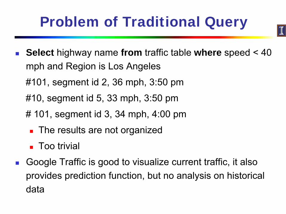
Problem of Traditional Query
Select highway name from traffic table where speed < 40 mph and Region is Los Angeles
#101, segment id 2, 36 mph, 3:50 pm
#10, segment id 5, 33 mph, 3:50 pm
# 101, segment id 3, 34 mph, 4:00 pm
The results are not organized
Too trivial
Google Traffic is good to visualize current traffic, it also provides prediction function, but no analysis on historical data
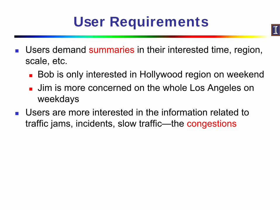
User Requirements
Users demand summaries in their interested time, region, scale, etc.
Bob is only interested in Hollywood region on weekendJim is more concerned on the whole Los Angeles on weekdays
Users are more interested in the information related to traffic jams, incidents, slow traffic—the congestions

Features of Traffic Data
Huge SizeThousands of road sensors, reporting the data in a time frequency of 30 secondsThe traffic databases contains Giga-bytes, even Tera-bytes of dataMost of them are normal records (the speed reading is close to the speed limit of the road)Congestions are dwarfed by normal data
Complex ObjectA congestion is a complex object with several road segments and varied time length – hard to model
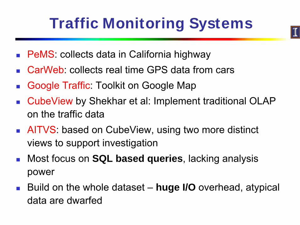
Traffic Monitoring Systems
PeMS: collects data in California highwayCarWeb: collects real time GPS data from carsGoogle Traffic: Toolkit on Google MapCubeView by Shekhar et al: Implement traditional OLAP on the traffic dataAITVS: based on CubeView, using two more distinct views to support investigationMost focus on SQL based queries, lacking analysis powerBuild on the whole dataset – huge I/O overhead, atypical data are dwarfed

Spatial/Traffic/Trajectory Data Cubes
Spatial Cube (Stefanovic et al. 2000)Dimension members are spatially referenced and can be represented on a Map
Trajectory Cube (Giannotti et al. 2007)include temporal, spatial, demo-graphic and techno-graphic dimensions, two kinds of measures: spatial measure and numerical measure
Flow Cube (Gonzalez et al. 2007)Analyzing item flows in RFID applications
Congestion Cube: On-going workMultidimensional analysis of traffic congestions
Congestion Event
A congestion is a dynamic process:start from a single segment of the streetsexpand along the road and influence nearby roadsmay cover hundred road segments when reaching the full sizeAs time passes by, those fragments shrink slowly and eventually disappear.
Group the congestion records that are spatially close and timely relevant to be a congestion event

Base Congestion Cluster
For each road segment in the congestion event, record the seg_id, total_duration and avg_speedCongestion Event:
Seg_1, 9:00 am, 30 mphSeg_2, 9:00 am, 35 mphSeg_1, 9:05 am, 40 mph…
Base Congestion ClusterSeg_1, 30 mins, 32.5 mphSeg_2, 20 mins, 35 mph

Congestion Cluster and Congestion Cube
Natural and distinguishableCongestion cube: Constructed based on congestion clusters

129
Part II. Traffic Data Mining
Introduction to Traffic Data
Traffic Data Warehousing
Route Discovery by Frequent Path Pattern
Analysis

130
Route Planning

131
Heuristic Shortest Path Algorithms for Transportation Networks (Fu et al.’06)
Problem
Route Guidance System (RGS)
Route Planning System (RPS)
Second level response, queries on large networks
Solution: Heuristic search
1. Limit Search Area
2. Search Decomposition
3. Limit Examined Links
132
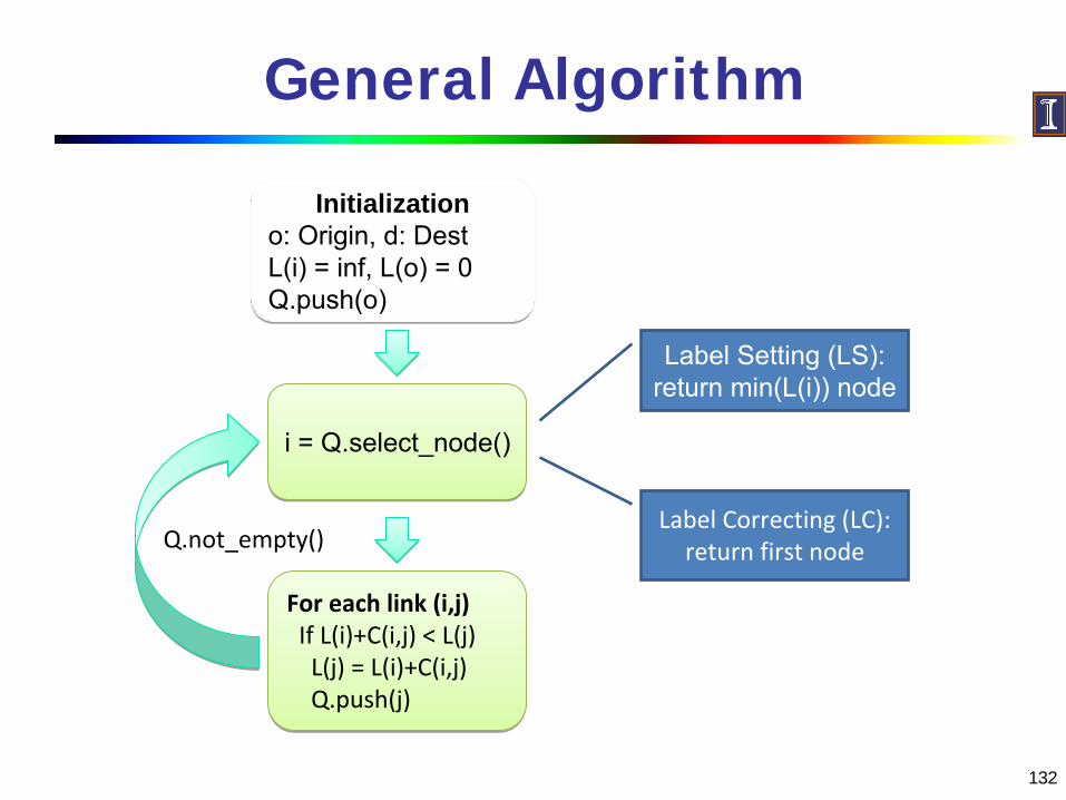
General Algorithm
Initializationo: Origin, d: DestL(i) = inf, L(o) = 0Q.push(o)
Initializationo: Origin, d: DestL(i) = inf, L(o) = 0Q.push(o)
i = Q.select_node()i = Q.select_node()
For each link (i,j)If L(i)+C(i,j) < L(j)L(j) = L(i)+C(i,j)Q.push(j)
For each link (i,j)If L(i)+C(i,j) < L(j)L(j) = L(i)+C(i,j)Q.push(j)
Q.not_empty()
Label Setting (LS):return min(L(i)) node
Label Correcting (LC):return first node

133
Method 1. Limit Search Area
Branch Pruning [Fu et al. 96, Karim 96]Q.select_node()
Select node if L(i) + e(i,d) < E(o,d)Prune unpromising nodesExpands: 20% of LS
A-Star [Hart 68, Nilsson 71]Select node with min L(i) + e(i,d)Prioritize promising nodesExpands: 10% of LS
Branch Pruning vs. A-Star
Dest.Origin
ExpandedLS
ExpandedLimited

134
Method 2. Search Decomposition
Algorithm cost grows faster than graph sizeDecompose problem
Subgoals[Bander et al. 91][Dillenburg et al. 95]
Bidirectional Search[Dantzig 60, Nicholson 66]
SubgoalsSubgoals
min e(i,d) min e(o,i)
135
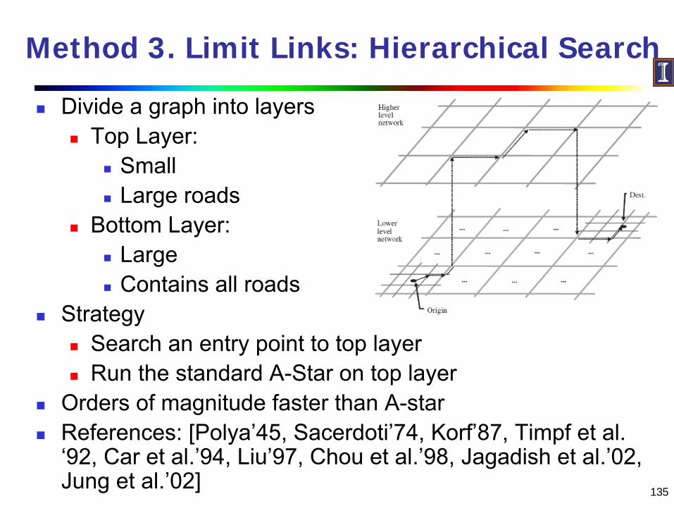
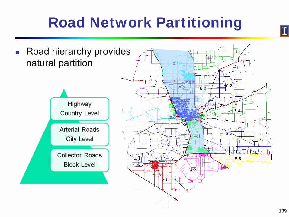
Method 3. Limit Links: Hierarchical Search
Divide a graph into layersTop Layer:
SmallLarge roads
Bottom Layer:LargeContains all roads
StrategySearch an entry point to top layerRun the standard A-Star on top layer
Orders of magnitude faster than A-starReferences: [Polya’45, Sacerdoti’74, Korf’87, Timpf et al. ‘92, Car et al.’94, Liu’97, Chou et al.’98, Jagadish et al.’02, Jung et al.’02]
136
Hierarchical Search
SpeedupLinear in search spaceOrders of magnitude faster than A-StarOnly viable option
Sub-optimal solutionPath 9% - 50% slower than optimalNo shortcuts between top/bottom layersBad for short trips
Better to avoid highways

137
Mining Frequent Routes: When in Rome, Do as the Romans Do
Adaptive Fastest Path Computation on a Road Network [Hector et al. 07]
Data is the King
No model can anticipate all variables
Fastest Route
Frequent Route

138
Mining for Fast and Popular Routes
Speed PatternsDriving Patterns
Query:Start: Node AEnd: Node BTime: T
Route Planning
Road Network
Fast but also
Popular
Fast but also
PopularNewNew
Driving ConditionsForecast
139
Road Network Partitioning
Road hierarchy provides natural partition
140
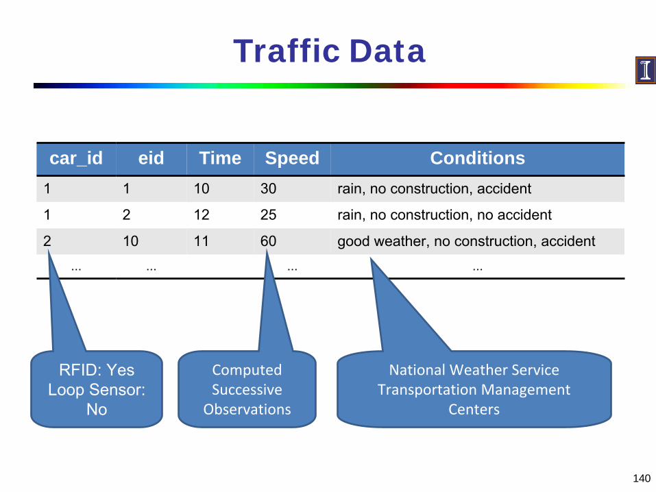
Traffic Data
car_id eid Time Speed Conditions1 1 10 30 rain, no construction, accident
1 2 12 25 rain, no construction, no accident
2 10 11 60 good weather, no construction, accident... ... ... ...
RFID: YesLoop Sensor:
No
National Weather ServiceTransportation Management
Centers
ComputedSuccessive
Observations

141
Mining Speed Patterns
Model of speed changesClassification
Given conditions predict speed (discrete)We use decision tree
Regression problemGiven conditions predict speed (continuous)
Area
Weather Time
A1A2
¼ 1
Icy Other
…
⅓
Rush
⅓
Normal

142
Mining Driving Patterns
For each area:Define minimum supportMine frequent trajectories
Length k: For RFID DataLength 1: For loop detectors
Driving Conditions Area Popular RoutesAll A1 {r1,r3,r5}
Snow A2 {r13,r29}Rush Hour, Any Weather A3 {r6,r6}

143
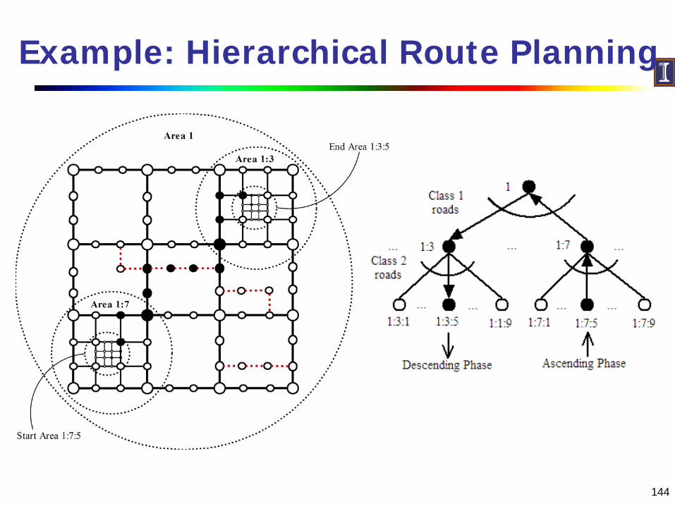
Hierarchical Route Planning
Ascending PhaseMove from start through successively bigger roads towards goal
Move only through large roadsDescending Phase
Move towards goal through successively smaller roadsAt each step
Select frequently traveled roadsUse dynamic speed model
144
Example: Hierarchical Route Planning

145
Result: San Joaquin Route
Shortest pathSuggested path

146
Summary: Traffic Data Mining
Traffic Warehousing
Congestion cluster based approach
Heuristic methods to mine significant clusters
Route Discovery
Heuristic methods (Limit Search Area, Search Decomposition, Limit Examined Links), adaptive method
Hot-Route Detection
FlowScan

147
Tutorial Outline
Part I. Mining Moving Objects
Part II. Mining Traffic Data
Part III. Conclusions

148
Conclusions
Mining moving object data, trajectory data and traffic data
are important tasks in data mining
Lots of rich and exciting results
This tutorial has presented an overview of recent
approaches in this direction
Promising research directions
Moving object/traffic mining in cyber-physical networks
Integration with heterogeneous information networks
Exploration of diverse applications

149
References: Moving Object Databases and Queries
R. H. Gueting and M. Schneider. Moving Objects Databases. Morgan Kaufmann, 2005.S. R. Jeffrey, G. Alonso, M.J. Franklin, W. Hong, and J. Widom. A pipelined framework for online cleaning of sensor data streams. ICDE'06.N. Jing, Y.‐W. Huang, and E. A. Rundensteiner. Hierarchical optimization of optimal path finding for transportation applications. CIKM'96.C. S. Jensen, D. Lin, and B. C. Ooi. Query and update efficient b+‐tree based indexing of moving objects. VLDB'04.E. Kanoulas, Y. Du, T. Xia, and D. Zhang. Finding fastest paths on a road network with speed patterns. ICDE'06.J. Krumm and E. Horvitz. Predestination: Inferring destinations from partial trajectories. Ubicomp'06.E. M. Knorr, R. T. Ng, and V. Tucakov. Distance‐based outliers: Algorithms and applications. The VLDB Journal, 8(3):237‐253, February 2000.L. Liao, D. Fox, and H. Kautz. Learning and inferring transportation routines. AAAI'04.

References on Moving Object Pattern Mining (I)
150
M. Andersson, Gudmundsson, J., Laube, P. & Wolle, T., "Reporting Leaders and Followers Among Trajectories of Moving Point Objects" , GeoInformatica, 2008.M. Benkert, J. Gudmundsson, F. Hubner, and T. Wolle. Reporting flock patterns. Euro. Symp. Algorithms’06.M. Benkert, J. Gudmundsson, F. Hubner, and T. Wolle. Reporting leadership patterns among trajectories. SAC'07.H. Cao, N. Mamoulis, and D. W. Cheung. Mining frequent spatiotemporal sequential patterns. ICDM'05.M. G. Elfeky, W. G. Aref, and A. K. Elmagarmid. Periodicity detection in time series databases. IEEE Trans. Knowl. Data Eng., 17(7), 2005.R. Fraile and S. J. Maybank. Vehicle trajectory approximation and classification. In Proc. British Machine Vision Conf., Southampton, UK, September 1998.F. Giannotti, M. Nanni, F. Pinelli, and D. Pedreschi. Trajectory pattern mining. KDD’07.S. Gaffney and P. Smyth. Trajectory clustering with mixtures of regression models. KDD'99.J. Gudmundsson and M. J. van Kreveld. Computing longest duration flocks in trajectory data. GIS’06.J. Gudmundsson, M. J. van Kreveld, and B. Speckmann. Efficient detection of patterns in 2d trajectories of moving points. GeoInformatica, 11(2):195‐215, June 2007.H. Jeung, M. L. Yiu, X. Zhou, C. S. Jensen and H. T. Shen, "Discovery of Convoys in Trajectory Databases", VLDB 2008.

References on Moving Object Pattern Mining (II)
151
P. Kalnis, N. Mamoulis, and S. Bakiras. On discovering moving clusters in spatiotemporal data. SSTD 2005.V. Kostov, J. Ozawa, M. Yoshioka, and T. Kudoh. Travel destination prediction using frequent crossing pattern from driving history. Proc. Int. IEEE Conf. Intelligent Transportation Systems, Vienna, Austria, Sept. 2005 Y. Li, J. Han, and J. Yang. Clustering moving objects. KDD'04.Z. Li, et al., “MoveMine: Mining Moving Object Databases", SIGMOD’10 (system demo)Z. Li, B. Ding, J. Han, and R. Kays, “Swarm: Mining Relaxed Temporal Moving Object Clusters”, in submissionZ. Li, B. Ding, J. Han, and R. Kays, “Mining Hidden Periodic Behaviors for Moving Objects”, in submissionN. Mamoulis, H. Cao, G. Kollios, M. Hadjieleftheriou, Y. Tao, and D. W. Cheung. Mining, indexing, and querying historical spatiotemporal data. KDD 2004..M. Nanni and D. Pedreschi. Time‐focused clustering of trajectories of moving objects. JIIS, 27(3), 2006.I. F. Sbalzariniy, J. Theriot, and P. Koumoutsakos. Machine learning for biological trajectory classification applications. In Proc. 2002 Summer Program, Center for Turbulence Research, August 2002.I. Tsoukatos and D. Gunopulos. Efficient mining of spatiotemporal patterns. SSTD'01.

References on Outlier Detection
152
E. Horvitz, J. Apacible, R. Sarin, and L. Liao. Prediction, expectation, and surprise:
Methods, designs, and study of a deployed traffic forecasting service. UAI'05
E. M. Knorr, R. T. Ng, and V. Tucakov. Distance‐based outliers: Algorithms and
applications. The VLDB Journal, 8(3):237‐253, February 2000.
J.‐G. Lee, J. Han, and X. Li, "Trajectory Outlier Detection: A Partition‐and‐Detect
Framework", ICDE 2008
J.‐G. Lee, J. Han, and K.‐Y. Whang, “Trajectory Clustering: A Partition‐and‐Group
Framework”, SIGMOD'07
X. Li, J. Han, S. Kim, "Motion‐alert: Automatic anomaly detection in massive
moving objects", ISI 2006
X. Li, J. Han, S. Kim, and H. Gonzalez, “ROAM: Rule‐ and Motif‐Based Anomaly
Detection in Massive Moving Object Data Sets”, SDM'07
J. Owens and A. Hunter. Application of the self‐organizing map to trajectory
classification. In . 3rd IEEE Int. Workshop on Visual Surveillance, Dublin, Ireland,
July 2000

References on Prediction and Classification
153
Faisal I. Bashir, Ashfaq A. Khokhar, Dan Schonfeld, View‐invariant motion trajectory‐based
activity classification and recognition, Multimedia Syst. (MMS) 12(1):45‐54 (2006)
R. Fraile and S. J. Maybank. Vehicle trajectory approximation and classification. In Proc.
British Machine Vision Conf., Southampton, UK, Sept. 1998
H. Jeung, Q. Liu, H. T. Shen, X. Zhou: A Hybrid Prediction Model for Moving Objects. ICDE
2008
J.‐G. Lee, J. Han, X. Li, and H. Gonzalez, “TraClass: Trajectory Classification Using
Hierarchical Region‐Based and Trajectory‐Based Clustering”, VLDB 2008.
Anna Monreale, Fabio Pinelli, Roberto Trasarti, Fosca Giannotti: WhereNext: a location
predictor on trajectory pattern mining. KDD 2009
I. F. Sbalzariniy, J. Theriot, and P. Koumoutsakos. Machine learning for biological trajectory
classification applications. In Proc. 2002 Summer Program, Center for Turbulence Research,
August 2002.
Y. Tao, C. Faloutsos, D. Papadias, B. Liu: Prediction and Indexing of Moving Objects with
Unknown Motion Patterns. SIGMOD 2004
Reference on Traffic MiningA. Awasthi, Y. Lechevallier, M. Parent, and J.‐M. Proth. Rule based prediction of fastest paths on urban networks. Intelligent Transportation Systems’05.J. Brusey, C. Floerkemeier, M. Harrison, and M. Fletcher. Reasoning about uncertainty in location identification with RFID. In Proc. Workshop on Reasoning with Uncertainty in Robotics at IJCAI‐2003.L. Bloomberg, V. Bacon, and A. May. Freeway detector data analysis: smart corridor simulation evauluation. In Technical Report UCB‐931, 1993.T. Choe, A. Skabardonis, and P. Varaiya. Freeway performance measurement system (pems): An operational analysis tool. In TRB, 2002.H. Gonzalez, J. Han, X. Li, M. Myslinska, and J. P. Sondag, “Adaptive Fastest Path Computation on a Road Network: A Traffic Mining Approach”, VLDB'07.X. Li, J. Han, J.‐G. Lee, and H. Gonzalez, “Traffic Density‐based Discovery of Hot Routes in Road Networks”, SSTD'07.C. Lu, A. P. Boedihardjo, and J. Zheng. Aitvs: Advanced interactive traffic visualization system. In ICDE, 2006.Z. Jia, C. Chen, B. Coifman, and P. Varaiya. The pems algorithms for accurate, real‐time estimates of g‐factors. In IEEE ITS Conference, 2001.C.‐H. Lo, W.‐C. Peng, C.‐W. Chen, T.‐Y. Lin, and C.‐S. Lin. Carweb: A traffic data collection platform. In MDM, 2008.S. Shekhar, C. Lu, R. Liu, and C. Zhou. Cubeview: A system for traffic data visualization. In ICITS, 2002.
154


