
Model identification for dose response signal
detection
Holger Dette, Stefanie Titoff,
Stanislav Volgushev
Ruhr-Universitat Bochum
Fakultat fur Mathematik
44780 Bochum, Germany
e-mail: [email protected]
Frank Bretz
Novartis Pharma AG
Lichtstrasse 35
4002 Basel, Switzerland
e-mail: [email protected]
August 27, 2012
Model identification for dose response signal detection
Abstract
We consider the problem of detecting a dose response signal if several competing
regression models are available to describe the dose response relationship. In particular,
we re-analyze the MCP-Mod approach from Bretz et al. (2005), which has become a
very popular tool for this problem in recent years. We propose an improvement based
on likelihood ratio tests and prove that in linear models this approach is always at least
as powerful as the MCP-Mod method. This result remains valid in nonlinear regression
models with identifiable parameters. However, for many commonly used nonlinear dose
response models the regression parameters are not identifiable and standard likelihood
ratio test theory is not applicable. We thus derive the asymptotic distribution of
likelihood ratio tests in regression models with a lack of identifiability and use this
result to simulate the quantiles based on Gaussian processes. The new method is
illustrated with a real data example and compared to the MCP-Mod procedure using
theoretical investigations as well as simulations.
Keywords and Phrases: dose response studies; nonlinear regression; model identification;
likelihood ratio test; contrast tests
1

1 Introduction
An important problem in the development of any new chemical or biological entity consists
of characterizing well its dose response relationship (Ruberg, 1995a,b; Bretz et al., 2008).
Statistical analysis methods of dose response studies can be roughly divided into (i) test pro-
cedures to detect a dose response signal (Stewart and Ruberg, 2000) or identify statistically
significant dose levels (Tamhane et al., 1997, 2001) and (ii) regression methods to estimate
the dose response curve. A common regression approach is to use a parametric dose response
model that assumes a functional relationship between dose, treated as a continuous variable,
and response (Morgan, 1992; Pinheiro et al., 2006b). If the parametric model is correctly
specified, maximum likelihood or least squares estimation is an efficient method. However,
misspecifying the parametric model can lead to substantial bias in estimating the dose re-
sponse curve. This creates a dilemma in practice, because it is often required to pre-specify
the parametric model, when the form of the dose response model in unknown. This is par-
ticularly true for the regulated environment in which drug development takes place, where
the analysis methods (including the choice of the dose response model) have to be defined
at the study design stage (ICH, 1994).
Many authors have investigated semi-parametric or non-parametric approaches to alleviate
the model dependency problem and enhance the robustness of the dose response estimation;
see Muller and Schmitt (1988); Kelly and Rice (1990); Mukhopadhyay (2000); Dette et al.
(2005); Bornkamp and Ickstadt (2009); Dette and Scheder (2010); Yuan and Yin (2011)
among many others. These methods allow model-independent descriptions of a dose response
relationship. However, their applicability in dose response studies is limited because they
require observations on a rather dense set of different dose levels, which are rarely available
in practice. Due to logistic and ethical reasons, the number of different dose levels is typically
in the order of 5 (Bornkamp et al., 2007) and therefore nonparametric methods do not yield
reliable results.
Extending initial ideas proposed by Tukey et al. (1985) to address model uncertainty, Bretz
et al. (2005) suggested a different strategy by choosing an appropriate model from a set
of pre-specified candidate parametric dose response models; see Table 1 for a typical set
of competing models used in practice. Their method, abbreviated as MCP-Mod, combines
multiple comparison procedures with modeling techniques and consists of two steps. To begin
with, it aims at detecting a dose response signal using multiple contrast tests. Conditional on
a statistically significant outcome, it then selects a suitable dose response model to produce
inference on adequate doses, employing a model-based approach. The MCP-Mod approach
has become a very popular tool in recent years and has been subject to several extensions.
Pinheiro et al. (2006a) discussed practical considerations regarding the implementation of
2
this methodology. Neal (2006) and Wakana et al. (2007) extended the original approach to
Bayesian methods estimating or selecting the dose response curve from a sparse dose design.
Klingenberg (2009) applied the MCP-Mod approach to proof-of-concept studies with binary
responses. Benda (2010) proposed a time-dependent dose finding approach with repeated
binary data. Akacha and Benda (2010) investigated the impact of dropouts on the analysis
with recurrent event data. Several authors investigated extensions of the original MCP-Mod
approach to response-adaptive designs; see Miller (2010); Bornkamp et al. (2011); Tanaka
and Sampson (2012).
In this paper we re-analyze the MCP-Mod procedure and suggest an improvement. Our
proposed approach is based on likelihood ratio tests and has at least two advantages. On
the one hand, it makes better use of the available information than the original MCP-
Mod procedure, because it uses the complete structure of the regression models. On the
other hand, it does not require knowledge of the parameters of the competing models which
are needed for the MCP-Mod procedure to construct the contrast tests for dose response
signal detection. A particular challenge when using the likelihood ratio approach is that for
commonly used regression models, such as those specified in Table 1, the resulting contrast
tests correspond to the problem of testing for a constant regression. This leads to the
problem of non-identifiability of some model parameters under the null hypothesis of no
dose response. Consequently, standard asymptotic theory for likelihood ratio tests is not
applicable here. In the context of independent and identically distributed observations such
theory has been developed by Lindsay (1995) and Liu and Shao (2003). However, to the
best knowledge of the authors, the asymptotic properties of the likelihood ratio test in the
case of a lack of identifiability and independent but not identically distributed observations
(in particular for regression models with fixed design) have not been investigated so far.
The remaining part of the paper is organized as follows. In Section 2 we revisit the original
MCP-Mod approach and introduce the corresponding likelihood ratio tests. In Section 3 we
compare both methods in the case of linear regression models. We show that if the number
of different dose levels coincides with the number of parameters in the regression model,
the MCP-Mod procedure is in fact a likelihood ratio test. More generally, we prove that in
linear models the likelihood ratio test is always at least as powerful as the original MCP-Mod
method and that the amount of improvement can be substantial. These results hold also
(at least asymptotically) in nonlinear models where all parameters are identifiable under
the null hypothesis of no dose response. However, the results of Song et al. (2009) indicate
that this is not necessarily the case under non-identifiability of the parameters. Therefore,
we develop in Section 4 a method to simulate the asymptotic distribution of the likelihood
ratio test under lack of identifiability of the parameters for independent non-identically
distributed data. In Section 5 we present some simulation results to illustrate the differences
3

model η(x, θ) (I) (II) (III)
linear ϑ1,1 + ϑ1,2x (0.2,0.6) (0.1,0.3) (0.2,0.6)
Emax ϑ2,1 +ϑ2,2x
ϑ2,3+x(0.2,0.7,0.2) (0.1,0.3,0.01) (0.2,0.612,0.021)
exponential ϑ3,1 + ϑ3,2 exp(x/ϑ3,3
)(0.183,0.017,0.28) (0.085,0.006,0.333) (0.005,0.195,0.712)
log-linear ϑ4,1 + ϑ4,2 log (x + ϑ4,3) (0.74,0.33,0.2) (0.392,0.098,0.05) (0.795,0.175,0.033)
Table 1: Common parametric dose response models, with different parameter specifications
(I) - (III).
between the two methods. In particular, we demonstrate that in the considered examples the
procedure based on likelihood ratio tests is never less powerful than the original MCP-Mod
approach. In Section 6 we illustrate the new methodology with a real data set and provide
some concluding remarks in Section 7. Finally, Section 8 contains some technical details
justifying the results from Section 3 and 4.
2 Preliminaries
We consider the common nonlinear regression model
Yij = η(xi, θ) + εij, i = 1, . . . , N, j = 1, . . . , ni,N∑i=1
ni = n, (2.1)
where η denotes the regression function, x1, . . . , xN are different experimental conditions and
ni observations are taken at xi, i = 1, . . . , N . In (2.1) the quantities εij denote independently
normally distributed random variables with mean 0 and variance σ2 > 0. We assume M ∈ Ncandidate models
η1(x, θ1), . . . , ηM(x, θM) (2.2)
to describe the regression, where θk ∈ Θk ⊂ Rdk denotes a dk-dimensional parameter in
the kth model, k = 1, . . . ,M . Throughout this paper the number of different experimental
conditions is fixed, such that
nin
= ξi + o(1), i = 1, . . . , N, (2.3)
where n =∑N
i=1 ni →∞ denotes the total sample size and ξ1, . . . , ξN positive weights with
sum 1. The described situation is motivated by our interest in dose response studies, where
patients are randomized to N dose levels and N is typically in the order of 4 or 5 due to
logistic reasons. The assumption (2.3) is introduced for the asymptotic analysis of likelihood
ratio tests in Section 4. We finally define ξ as the probability measure, which puts mass ξiat the point xi, i = 1, . . . , N .
4

2.1 The MCP-Mod procedure revisited
As stated in the Introduction, Bretz et al. (2005) proposed the MCP-Mod approach to ana-
lyze dose response data under model uncertainty. First, the MCP-Mod approach investigates
whether a given compound has a dose dependent effect. Second, it selects an appropriate
model from the candidate model set (2.2) that most likely describes the underlying dose
response curve.
Bretz et al. (2005) defined for each dose response model under consideration the vector
µk = (µk,1, . . . , µk,N)T , (2.4)
where for k = 1, . . . ,M and i = 1, . . . , N the quantity µk,i = ηk(xi, θk) denotes the expecta-
tion of Yij in model (2.1) if ηk is the “correct” model. That is, the vector µk describes the
average effect of the compound at the experimental conditions x1, . . . , xN , if the model ηk is
the true one.
Bretz et al. (2005) proposed to test for each model the hypothesis
H0,k : cTk µk = 0 against H1,k : cTk µk > 0 (2.5)
for a given contrast vector ck = (ck,1, . . . , ck,N)T ∈ RN using the test statistic
Kn,k =cTk Y√
σ2∑N
i=1 c2k,i/ni
, k = 1, . . . ,M. (2.6)
Here, YT
= (Y 1, . . . , Y N) denotes the vector of means Y i =∑ni
j=1 Yij/ni at the dose levels
xi (i = 1, . . . , N) and σ2 = 1N−n
∑Ni=1
∑nij=1(Yij − Y i)
2 is an estimator of the variance. Note
that under the null hypothesis H0,k : cTk µk = 0 the statistic Kn,k has a central t-distribution
with n−N degrees of freedom, while under the alternative it has a non-central t distribution
with non-centrality parameter
τk(c) =cTk µk√
σ2∑N
i=1 c2k,i/ni
. (2.7)
Bretz et al. (2005) determined for each candidate dose response model an optimal contrast
c∗k maximizing τ 2k (c) in the class of all contrasts. These contrasts are then used in the test
statistics (2.6). Note that the optimal contrasts depend on the particular model under con-
sideration (in particular on the unknown model parameters) and the experimental conditions
x1, . . . , xN .
5

In order to conclude in favor of a statistically significant dose response signal, the M individ-
ual contrast test statistics Kn,k are combined into a single decision rule. Bretz et al. (2005)
suggested using the maximum statistic
Kn,max =M
maxk=1
Kn,k, (2.8)
where critical values are obtained from a multivariate t-distribution (Genz and Bretz, 2009).
If statistical significance is achieved at this step, the MCP-Mod approach proceeds with
selecting a suitable dose response model and fitting it to the data before estimating the
target dose(s) of interest based on the fitted model. In this paper we mainly investigate the
first step of the MCP-Mod procedure and propose a more powerful test to detect a dose
response signal.
2.2 Likelihood ratio tests
A natural alternative to the contrast tests used by Bretz et al. (2005) is an approach based
on likelihood ratio (LR) tests. In the following discussion let ‖ · ‖2 denote the Euclidean
norm. The LR test statistics for the hypotheses in (2.5) are given by
LRn,k = −2 logT kn,H0
T kn,H1
, k = 1, . . . ,M, (2.9)
where
T kn,H0= sup
{ 1
σnexp(− 1
2σ2‖Y − ηk(θk)‖2
2
)∣∣∣ σ > 0; θk ∈ Rdk ; cTk µk = 0},
T kn,H1= sup
{ 1
σnexp(− 1
2σ2‖Y − ηk(θk)‖2
2
)∣∣∣ σ > 0; θk ∈ Rdk ; cTk µk ≥ 0}.
Here, Y = (Yij)j=1,...,nii=1,...,N ∈ Rn and ηk(θk) = (η(xij, θk)
j=1,...,nii=1,...,N ∈ Rn denote the vectors of
observations and expected responses at the different dose levels in the kth model, respectively.
The LR test rejects the null hypothesis (2.5) of no dose response for large values of the
statistic LRn,k. The analogue of the statistic (2.8) is given by
LRn,max =M
maxk=1
LRn,k, (2.10)
where critical values have to be found by asymptotic theory in most cases of practical interest.
In classical likelihood theory the statistic LRn,k usually converges weakly to a chi-squared
type distribution, provided that the parameters characterizing the null distribution are
unique [Wilks (1938) or Chernoff (1954)]. On the other hand, it is well known that classical
6

likelihood ratio theory does not apply to problems with a loss of identifiability [see Prakasa-
Rao (1992), Lindsay (1995), Liu and Shao (2003) or Song et al. (2009) among others]. In
the examples of Table 1 the problem of non-identifiability under the null hypothesis occurs
naturally when testing the null hypothesis H0,k : ϑk,2 = 0 in the kth model.
In the following sections we will compare the contrast test used in the original MCP-Mod
method with the LR test proposed here. We begin the discussion with linear models for
which the situation is most transparent. In this case the parameters are identifiable. The
LR approach is always at least as good as the contrast test and the amount of improvement
can be substantial. These results hold also in case of nonlinear regression models with
identifiable parameters. For regression models with lack of identifiability the asymptotic
distribution of the LR test has not been considered so far in the literature and will be
presented in Section 4.
3 LR tests and MCP-Mod in linear regression models
For the sake of simplicity, we consider the test problem (2.5) for a single linear regression
model
Yij = fT (xi)θ + εij, j = 1, . . . , ni, i = 1, . . . , N, (3.1)
with parameter vector θ ∈ Rd, where f is a given vector of regression functions. The results
derived in this section can then be applied to each of the k test problems discussed in Section
2.
Because we consider only a single model, we use for now the notation µT = (µ1, . . . , µN) and
cT = (c1, . . . , cN) instead of µk and ck. Let
XT = (f(x1), . . . , f(x1), . . . , f(xN), . . . , f(xN)) ∈ Rd×n (3.2)
denote the corresponding design matrix, where each vector f(xi) appears exactly ni times
in the matrix XT and n =∑N
i=1 ni. We also assume that XT has rank d, which means that
there exist d linearly independent vectors f(xi1), . . . , f(xid) among f(x1), . . . , f(xN). It is
easy to see that the vector µ in (2.4) can be represented in the form µ = AXθ, where
AT = diag( 1
n1
1n1 ,1
n2
1n2 , . . . ,1
nN1nN)∈ Rn×N , (3.3)
1k ∈ Rk denotes the vector with all entries given by 1 and all other entries in the matrix AT
are 0. In linear models with normally distributed homoscedastic errors the LR test statistic
7

(2.9) for the hypotheses in (2.5) specializes to Tn,H0 and Tn,H1 are defined by
Tn,H0 = sup{ 1
σnexp(− 1
2σ2‖Y −Xθ‖2
2
) ∣∣∣ σ > 0; θ ∈ Rd; cTµ = 0}, (3.4)
Tn,H1 = sup{ 1
σnexp(− 1
2σ2‖Y −Xθ‖2
2
) ∣∣∣ σ > 0; θ ∈ Rd; cTµ ≥ 0}.
It now follows by straightforward calculation using Lagrangian multipliers that
ne−1 · (Tn,H0)−2/n = ‖Y −Xθ‖2
2 +(cT (XTX)−1XTY )2
cT (XTX)−1c,
where Y = (Y11, . . . , Y1n1 , . . . , YN1, . . . , YNnN )T is the vector of all observations, c = XTAT c
and θ = (XTX)−1XTY is the usual least squares estimate. Similarly, we have
ne−1 · (Tn,H1)−2/n = ‖Y −XθH1‖2
2, (3.5)
where θH1 denotes the maximum likelihood estimate under the assumption cTµ = cT θ ≥ 0;
see the derivation in Section 8.1 of the Appendix. We thus have
θH1 =
{θ = (XTX)−1XTY if cT θ = cTAXθ > 0
θH0 = (XTX)−1XTY − λ(XTX)−1XTAT c if cT θ = cTAXθ ≤ 0,
where θH0 denotes the maximum likelihood estimate under the null hypothesis cTµ = 0 and
λ =cT (XTX)−1XTY
cT (XTX)−1c=
cTAX(XTX)−1XTY
cTAX(XTX)−1XTAT c. (3.6)
This gives for the LR test in (2.9), up to a monotone transformation,
Ln =
0 if cT θ ≤ 0
(cT (XTX)−1XTY )2
cT (XTX)−1c‖Y −Xθ‖22
if cT θ > 0.(3.7)
Consequently, the LR test rejects the null hypothesis (2.4) in the linear model (3.1) for large
values of the statistic
`n =cT θ
‖Y −Xθ‖2(cT (XTX)−1c)1/2. (3.8)
Theorem 3.1 For the linear regression model (3.1) with N = d different experimental
conditions, the LR test statistic (3.8) and the contrast test statistic (2.6) coincide up to a
constant factor.
8

Note that the assumption d = N is crucial for Theorem 3.1. If the number of different
experimental conditions is larger than the number of parameters in the linear model, the
LR test can be more powerful than the contrast test. In many cases the improvement is
substantial, as illustrated in the following example.
Example 3.1 Consider the model η(x, θ) = ax and the case N = 2, where observations
are taken at two different experimental conditions, say x1, x2, where x2 > x1. In this case,
contrast coefficients are uniquely determined (up to the sign) and we have c = (−1, 1)T/√
2.
The test statistic in (2.6) becomes
Kn =Y 2 − Y 1√σ2( 1
n1+ 1
n2)
and follows a t-distribution with n − 2 degrees of freedom if a = 0. We reject the null
hypothesis in (2.5) whenever Kn > tn−2,1−α, where tn−2,1−α denotes the (1 − α)-quantile
of the t-distribution with n − 2 degrees of freedom. Moreover, let Φ denote the standard
normal distribution function. Since cTµ = a(x2 − x1)/√
2, the power of this contrast test is
approximately given by
PcTµ>0(Kn > tn−2,1−α) ≈ Φ(aσ
(x2 − x1)
√n1n2
n1 + n2
− u1−α
), (3.9)
where u1−α denotes the (1− α)-quantile of the standard normal distribution.
Consider now the LR test and note that d = 1, which implies c ∈ R. Therefore, the LR test
(3.8) rejects the null hypothesis in (2.5) whenever
Ln =n1x1Y 1 + n2x2Y 2
σ(n1x21 + n2x2
2)1/2> tn−1,1−α,
where the estimator of the variance is now given by
σ2 =2∑i=1
ni∑j=1
(Yij −
n1x3−i1 xi−1
2 Y 1 + n2x2−i1 xi2Y 2
n1x21 + n2x2
2
)2
.
The power of this test is approximately given by
PcTµ>0(Ln > tn−1,1−α) ≈ Φ(a(n1x
21 + n2x
22)
σ
1/2
− u1−α
). (3.10)
Since (x2− x1)√
n1n2
n1+n2≤√n1x2
1 + n2x22 for all x2 > x1, it follows that the LR test is always
more powerful than the contrast test. The power difference can be rather substantial. For
example, if x1 = 1, x2 = 2, and n1 = n2, the power in (3.9) becomes Φ( aσ
√n√2− u1−α), while
the corresponding term in (3.10) is Φ( aσ
√10√n√2− u1−α). Thus, in this example the LR test
gives approximately the same power as the contrast test using only 10% of the sample size.
9

We now discuss a more general result showing the general superiority of the LR test in case
of linear models. For a precise statement we assume that the variance σ2 is known. A cor-
responding statement in cases where the variance has to be estimated holds asymptotically,
as indicated in the previous example.
If the variance is known, the LR test rejects the null hypothesis in (2.5) if
`n(σ2) =cT θ
σ(cT (XTX)−1c)1/2> u1−α, (3.11)
where c = XTAT c and the matrices XT and AT are defined in (3.2) and (3.3), respectively.
The corresponding contrast test rejects whenever
kn(σ2) =cTY
σ√∑N
i=1 c2i /ni
> u1−α. (3.12)
Our next results shows that in linear regression models with known variance the LR test is
at least as powerful as the contrast test, regardless of the choice of the contrast vector. For
an unknown variance these results hold at least if the sample size is sufficiently large (see
Example 3.2 below).
Theorem 3.2 Consider the linear regression model (3.1) with known variance. Whenever
cTµ ≥ 0 we have
P (`n(σ2) > u1−α) ≥ P (kn(σ2) > u1−α). (3.13)
Moreover, the inequality is strict if and only if AT c 6∈ range(X), where the matrix AT is
defined in (3.3).
Example 3.2 Consider the linear regression model η(x, θ) = ϑ0 + ϑ1x with equal sample
sizes n1 = . . . = nN = m. Up to the sign, the optimal contrast is given by
c∗ =( xi − x
(∑N
j=1(xj − x)2)1/2
)Ni=1, (3.14)
where x = 1N
∑Nj=1 xj (Bretz et al., 2005). Thus,
AT c∗ =( N∑j=1
(xj − x)2)−1/2
(1Tm(x1 − x), . . . , 1Tm(xN − x))T
∈ range(X) = {a1n + b (1Tmx1, . . . , 1Tmxm)T | a, b ∈ R}.
Consequently, by Theorem 3.2 the LR test and the optimal contrast test have the same
power. Note that this result holds also if the number of different experimental conditions
10

exceeds the dimension of the parameter. However, if a different contrast vector is used, the
range inclusion is not necessarily satisfied and the LR rest is usually more powerful.
In the following we report the results of a small simulation study to illustrate these facts.
We assume the models η(x) = 0.2 and η(x) = 0.2 + 0.6x under the null and the alternative
hypothesis, respectively. Further, we generated data with standard deviation σ = 1.478,
while the sample size is n = 200 with n1 = . . . = nN . All results are based on 5000 simulation
runs. The simulated level and power of the LR and contrast tests (with estimated standard
deviation) are shown in Table 2. The observed differences between the two methods are
within the simulation error, as predicted by Theorem 3.1.
Design LR test contrast test
x1 x2 level power level power
0 0.2 0.0436 0.1436 0.0446 0.1426
0 0.5 0.0522 0.4214 0.0494 0.4096
0 1 0.0568 0.8852 0.0470 0.8810
Table 2: Level and power of the LR and contrast tests for N = 2.
Next, we consider N = 4 different experimental conditions and the three different contrasts
c∗, c1 = (−1,−1, 1, 1)T , and c2 = (−1, 0, 0, 1)T , (3.15)
where c∗ denotes the optimal contrast defined in (3.14). Table 3 displays the simulation
results. Note that for all three contrasts under consideration the hypotheses (2.5) are equiv-
alent to H0 : ϑ1 = 0 and H1 : ϑ1 > 0 and therefore only one LR test is displayed in Table
3. In fact, one can show after tedious calculations that all vectors yield the same LR test
statistic in (3.7). The LR test is more powerful than the contrast tests based on c1 and c2,
as they do not satisfy the range inclusion in Theorem 3.2. For the optimal contrast test
based on c?, however, we observe no power difference compared with the LR test. Note that
this accordance is a specific coincidence of the linear regression model ϑ0 + ϑ1x used in this
example.
Design LR test contrast test
x1 x2 x3 x4 level power level power
c? c1 c20 0.05 0.1 0.2 0.0522 0.1100 0.0536 0.1078 0.0988 0.1080
0 0.1 0.4 0.5 0.0540 0.3288 0.0506 0.3206 0.2994 0.2666
0 0.25 0.75 1 0.0494 0.7342 0.0482 0.7414 0.6902 0.6464
Table 3: Level and power of the LR and contrast tests for N = 4.
In the case of nonlinear regression models the superiority of the LR test holds at least
asymptotically, provided that all parameters of the model are identifiable. This follows by
11

the usual linearization arguments [see Seber and Wild (1989)]. In the case of a lack of
identifiability, however, the results of Song et al. (2009) indicate that the superiority of the
LR test is not granted. We will investigate this in more detail in Section 4. We complete
this section with a nonlinear regression example satisfying the identifiability condition.
Example 3.3 Consider the model
η(x, θ) = ϑ0 − e−ϑ1x; ϑ0 ∈ R, ϑ1 ∈ R+0
with N = 2 different experimental conditions. In this case the contrast vector c is propor-
tional to (−1, 1) and we obtain for x1 < x2 cTµ = c−ϑ1x1 − e−ϑ1x2 . Therefore the hypothesis
(2.5) is equivalent to H0 : ϑ1 = 0 versus H1 : ϑ1 > 0. Table 4 displays the simulated level
and power of the LR and contrast tests, again for a sample size of n = 200, n1 = n2 and
σ = 1.478. We observe that both tests have very similar power properties. Next we consider
Design LR test contrast test
x1 x2 level power level power
0 1 0.0502 0.2306 0.0472 0.2206
0 2 0.0502 0.4780 0.0484 0.4666
0 5 0.0482 0.9106 0.0484 0.9148
Table 4: Level and power of the LR and contrast tests for N = 2.
the case of N = 4 with the contrasts c1 and c2 given in (3.15) and the optimal contrast c∗.
Table 5 displays the simulation results. We observe substantial power advantages for the LR
for the two contrasts c1, c2 and a similar behaviour for the optimal contrast c∗.
Design LR test contrast test
x1 x2 x3 x4 level power level power
c? c1 c20 0.25 0.75 1 0.0496 0.1720 0.0456 0.1638 0.1592 0.1398
0 0.5 1 2 0.0566 0.3154 0.0504 0.2974 0.2542 0.2876
0 1 3 5 0.0514 0.7540 0.0504 0.7524 0.6968 0.6900
Table 5: Level and power of the LR and contrast tests for N = 4.
4 LR tests under lack of identifiability
In this section we investigate the asymptotic distribution of the LR test for the hypotheses
in (2.5) under more general dose response models, such as those presented in Table 1. To
begin with, we demonstrate that under the null hypothesis of no dose response certain model
parameters are not identifiable and standard LR test theory is not applicable. Nevertheless,
we show in Section 8.2 of the Appendix that the quantiles of the limiting distribution can be
12

obtained using non-standard asymptotic theory for LR tests in regression models with a lack
of identifiability. These results are used in Section 4.2 where we explain how the quantiles
of the limiting process can be obtained by simulation.
4.1 The problem of identifiability
All models from Table 1 can be written as a nonlinear regression model of the form
η(x, θ) = ϑ0 + ϑ1η(x, θ(2)), (4.1)
where θ = (ϑ0, ϑ1, θT(2))
T ∈ Rd and θ(2) = (ϑ2, . . . , ϑd−1)T ∈ Rd−2. Assume without loss of
generality that we are interested in an increasing trend ϑ1 ≥ 0, i.e. η(x1, θ(2)) ≤ . . . ≤η(xN , θ(2)) for x1 < x2 < ... < xN . Using the Lagranges multiplier device and letting
µ = 1n
∑Ni=1 niµi, one can show by similar arguments as in (Bornkamp, 2006, p. 88) that the
solution of
c∗` = n`µ` − µ∑Ni=1 c
∗iµi
, ` = 1, . . . , N, (4.2)
maximizes the non-centrality parameter τ 2k (c) in (2.7) and is thus optimal. Note that τ 2
k (c)
is invariant with respect to scalings of the vector c and that c∗ satisfies∑N
`=1
(c∗` )2
n`= 1. Since
µ` = ηk(x`, θ), we have
c∗` = n`ηk(x`, θ)− η∑N
i=1 c∗iµi
= ϑ1n`η(x`, θ(2))− η∑N
i=1 c∗iµi
,
where η = 1n
∑N`=1 n`η(x`, θ) and η = 1
n
∑N`=1 n`η(x`, θ(2)). From the normalizing condition
it finally follows that
c∗` =ϑ1
|ϑ1|n`(η(x`, θ(2))− η)(∑N
i=1 ni(η(xi, θ(2))− η)2)1/2
, ` = 1, . . . , N.
Since we assumed ϑ1 ≥ 0, we obtain
c∗Tµ = ϑ1
N∑`=1
c∗` η`(x`, θ(2)) = ϑ1 ·( N∑i=1
n`(η(x`, θ(2))− η)2)1/2
.
Using the optimal contrast for the hypotheses in (2.5) under model (4.1) is thus equivalent
to testing the hypotheses
H0 : ϑ1 = 0 versus H1 : ϑ1 > 0. (4.3)
Therefore, the parameter θ(2) is not identifiable under the null hypothesis H0 : ϑ1 = 0
whenever d > 2. Nevertheless, the quantiles for the corresponding likelihood ratio test can
13

be obtained by non-standard asymptotic theory. Because these arguments are complicated,
we defer the detailed discussion to Section 8.2 in the Appendix and explain in the following
section how the quantiles of the asymptotic distribution of the likelihood ratio test can be
calculated numerically by simulating non-standard Gaussian processes.
4.2 Simulating quantiles
We assume that the vector θ(2) varies in some set, say Ψ, and define Z1, . . . , ZN , Y1, . . . , YNas independent identically distributed standard normal random variables. It is shown in
Section 8.2 that the asymptotic distribution of the likelihood ratio test for the hypothesis
(4.3) can be described by a functional of the stochastic process
{WS =W(β0, β1, σ, θ(2)) | β2
0 + β21 + σ2 = 1, β1 ≥ 0, σ > 0, θ(2) ∈ Ψ},
where S = (β0, β1, σ, θ(2)) and
WS =W(β0, β1, σ, θ(2)) =
∑Ni=1
√ξi((β0 + β1η(xi, θ(2)))Zi +
√2σYi)
(∑N
i=1 ξi(β0 + β1η(xi, θ(2))2 + 2σ2))1/2. (4.4)
To be precise, define
M2 ={
(β0, β1, σ, θ(2)) ∈ Rd+1∣∣∣β2
0 + β21 + σ2 = 1, β1 ≥ 0, θ(2) ∈ Ψ
},
M1 ={
(β0, 0, σ, θ(2)) ∈ Rd+1∣∣∣ β2
0 + σ2 = 1}.
It is shown in the Appendix that under the null hypothesis (4.3) the LR statistic converges
weakly to the random variable
L = supS∈M2
(WS ∨ 0)2 − supS∈M1
(WS ∨ 0)2. (4.5)
The quantiles of this limiting distribution can now be obtained by simulation.
So far, we focused on the specific case of testing a single model. In general, if M competing
models are considered and the test statistic (2.10) is used, the corresponding quantile can be
simulated in a similar way as described above. At each simulation step and for each model
ηk under consideration a random variable Lk defined in (4.5) is simulated on the basis of the
same data Z1, . . . , ZN , Y1, . . . , YNi.i.d∼ N (0, 1), resulting in the simulated random variable
Lmax =M
maxk=1
Lk. (4.6)
The quantiles of the limiting distribution of the statistic (2.10) are then calculated by re-
peating this simulation step 10.000 times, say. Note that the resulting quantiles depend on
14

statistic
designs Kn,max Lmax
total sample size
x1 x2 x3 x4 x5 n = 50 n = 125 n = 250
A 0 0.05 0.2 0.6 1 1.91719 1.90372 1.88322 3.84865
B 0 0.05 0.1 0.2 0.5 1.87306 1.83116 1.81475 3.93500
C 0.5 0.7 0.9 0.95 1 1.79709 1.78592 1.77634 3.16702
Table 6: Simulated 95%-quantiles of the statistic Kn,max defined in (2.8) and simulated 95%-
quantiles of the random variable Lmax defined in (4.6)
the models and the design under consideration. Exemplarily we display in Table 6 these
quantiles for the models from Table 1 and three uniform designs A, B, C with five different
experimental conditions each. Table 6 also contains the quantiles of the statistic (2.8) for
different values of n, based on the multivariate t-distribution with n− 5 degrees of freedom.
5 Simulation study
In this section we compare via a simulation study the original MCP-Mod from Bretz et al.
(2005) using contrast tests with a modified version using the LR tests developed in this
paper. We focus on the first step of the MCP-Mod approach, where the statistics (2.8) and
(2.10) are used to test the null hypothesis in (2.5). We investigate the three designs A, B
and C from Table 6. We use the four models in Table 1 as the candidate models for both
procedures. These four models plus the constant model serve also as the data-generating
“true” models in the simulations. The residual errors in (2.1) are normal distributed with
standard deviation σ = 1.478. All results are based on 5.000 simulation runs.
In Table 7 we display the power for both tests and various sample sizes for each of the five
data-generating regression models. The data were generated under the scenario (I) from
Table 1. Note that the statistic (2.8) requires the specification of the optimal contrasts c∗kand we used the “true” parameter values for their calculation. The LR test does not require
this knowledge.
For all designs the nominal level is well approximated by the (asymptotic) LR test. For the
contrast test, the significance level is maintained by construction also for finite sample sizes.
In terms of power, we do not observe substantial differences between both procedures. Only
if the true model is the Emax one, the LR test has slightly more power than the contrast
test. Note that the power to detect the Emax model for design C is generally very small
because of the choice of an inefficient design: observations are only taken at points larger
than 0.5. In this region the derivative varies between 0.1 and 0.25 and the function is almost
not distinguishable from the constant function.
Because the contrast test requires the knowledge of the model parameters for the calculation
15

true regression function
design test n constant Emax log-linear linear exponential
50 0.0536 0.2444 0.2742 0.2772 0.2684
contrast 125 0.0440 0.4718 0.4958 0.5034 0.4784
A 250 0.0566 0.7280 0.7706 0.7692 0.7636
50 0.0546 0.2710 0.3084 0.2802 0.2666
LR 125 0.0548 0.4936 0.5186 0.5104 0.4820
250 0.0586 0.7468 0.7672 0.7622 0.7396
50 0.0532 0.1840 0.1586 0.1294 0.0606
contrast 125 0.0570 0.3450 0.2834 0.1862 0.0840
B 250 0.0580 0.5508 0.4522 0.2994 0.0988
50 0.0520 0.1944 0.1628 0.1262 0.0670
LR 125 0.0488 0.3346 0.2662 0.1794 0.0780
250 0.0534 0.5454 0.4224 0.2750 0.0872
50 0.0498 0.0650 0.0952 0.1336 0.2212
contrast 125 0.0454 0.0744 0.1204 0.2028 0.4002
C 250 0.0470 0.0828 0.1756 0.3206 0.6428
50 0.0602 0.0688 0.1038 0.1362 0.2472
LR 125 0.0474 0.0856 0.1304 0.2180 0.4146
250 0.0546 0.0940 0.1714 0.3274 0.6422
Table 7: Power of the MCP-Mod procedure based on the LR test (2.10) and the contrast
test (2.8) at level 5%. Data was generated according to the constant model and the four
regression models from scenario (I) in Table 1. The “true” parameters have been used for
the calculation of the optimal contrasts in MCP-Mod.
true regression function
design n constant Emax log-linear linear exponential
50 0.0524 0.2462 0.2396 0.2450 0.2236
A 125 0.0482 0.4598 0.4744 0.4652 0.4286
250 0.0478 0.7122 0.7520 0.7444 0.7136
50 0.0464 0.1786 0.1470 0.1116 0.0588
B 125 0.0552 0.3234 0.2584 0.1770 0.0674
250 0.0500 0.5348 0.4208 0.2594 0.0856
50 0.0520 0.0702 0.0918 0.1196 0.2156
C 125 0.0526 0.0818 0.1236 0.2034 0.4110
250 0.0468 0.0934 0.1840 0.3404 0.6534
Table 8: Power of the MCP-Mod procedure based on the contrast test (2.8) at level 5%.
data were generated according to the constant model and four “true” regression models from
scenario (I) of Table 1. The parameters from scenario (II) have been used for the calculation
of the optimal contrasts in MCP-Mod.
16

of the optimal contrasts, we also investigate the properties of both tests if the contrasts are
misspecified due to wrong assumptions about the model parameters. In our first example
we generated data according to the same models as in Table 7, but with the contrasts being
slightly misspecified based on the parameters from scenario (II) in Table 1. Table 8 displays
the power results for the contrast test. The results for the LR test reported in Table 7 remain
the same because the data were generated according to the same models in both tables. In
almost all cases we observe a slight decrease in power for the contrast test as compared to
the LR test.
Finally, we study a further case of misspecification, where we generated data according to
scenario (III) in Table 1, while the optimal contrasts were calculated for the parameter
constellations given in scenario (I). Table 9 displays these results. We observe no power
differences between both procedures under design C. On the other hand, for designs A and
B the LR test approach is more powerful in most cases under consideration, in particular
for the Emax model.
true regression function
design test n constant Emax log-linear linear exponential
50 0.0488 0.1958 0.2480 0.2688 0.2698
contrast 125 0.0504 0.3674 0.4686 0.4954 0.5000
A 250 0.0534 0.5990 0.7328 0.7758 0.7553
50 0.0574 0.2548 0.2788 0.2928 0.2846
LR 125 0.0614 0.4914 0.4932 0.4984 0.5070
250 0.0590 0.7516 0.7414 0.7540 0.7552
50 0.0472 0.1762 0.1692 0.1202 0.0886
contrast 125 0.0510 0.3448 0.3092 0.1962 0.1376
B 250 0.0534 0.5630 0.5192 0.3062 0.1842
50 0.0496 0.2356 0.1932 0.1192 0.0864
LR 125 0.0516 0.4488 0.3264 0.1792 0.1188
250 0.0544 0.6998 0.5176 0.2728 0.1706
50 0.0562 0.0512 0.0754 0.1272 0.1812
contrast 125 0.0482 0.0506 0.0908 0.2094 0.2976
C 250 0.0498 0.0546 0.1188 0.3202 0.4802
50 0.0572 0.0600 0.0900 0.1572 0.1860
LR 125 0.0554 0.0567 0.0944 0.2188 0.3088
250 0.0478 0.0572 0.1159 0.3256 0.4882
Table 9: Power of the MCP-Mod procedure based on the LR test (2.10) and the contrast test
(2.8) at level 5%. Data were generated according to the constant model and the 4 regression
models from scenario (III) in Table 1. The parameters from scenario (I) have been used for
the calculation of the optimal contrasts in MCP-Mod.
6 A real dose finding trial example
In this section we illustrate the proposed LR test with a real dose finding trial example.
Biesheuvel and Hothorn (2002) investigated a dose ranging trial on a compound for the
treatment of the irritable bowel syndrome. Patients were randomized to either placebo or one
17
of four active dose levels, corresponding to doses 0, 1,2,3, and 4. Note that the original dose
levels have been blinded for confidentiality. The primary endpoint was a baseline adjusted
abdominal pain score with larger values corresponding to a better treatment effect. In total
369 patients completed the study, with nearly balanced allocation across the doses. For
the purpose of the calculations below, we ignore the gender information and investigated
dose response for the complete data set. The data are available, for example, with the
DoseFinding package from Bornkamp et al. (2010).
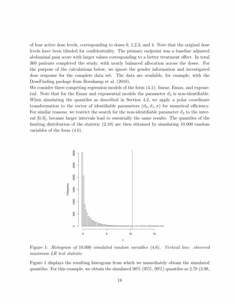
We consider three competing regression models of the form (4.1): linear, Emax, and expone-
tial. Note that for the Emax and exponential models the parameter ϑ2 is non-identifiable.
When simulating the quantiles as described in Section 4.2, we apply a polar coordinate
transformation to the vector of identifiable parameters (ϑ0, ϑ1, σ) for numerical efficiency.
For similar reasons, we restrict the search for the non-identifiable parameter ϑ2 to the inter-
val [0, 6], because larger intervals lead to essentially the same results. The quantiles of the
limiting distribution of the statistic (2.10) are then obtained by simulating 10.000 random
variables of the form (4.6).
x
Fre
quen
cy
0 5 10 15
050
010
0015
0020
0025
0030
00
Figure 1: Histogram of 10.000 simulated random variables (4.6). Vertical line: observed
maximum LR test statistic
Figure 1 displays the resulting histogram from which we immediately obtain the simulated
quantiles. For this example, we obtain the simulated 90% (95%, 99%) quantiles as 2.78 (3.98,
18

6.86). The observed maximum LR test statistic (2.10) for the given data is 10.3844, which
is displayed as a vertical line in Figure 1. Thus, we can safely reject the null hypothesis and
conclude in favor of a significant dose response signal. We obtain the same test decision by
computing the associated p-value, which is 0.0015 in this example
7 Conclusions
A common problem in modeling dose response relationships is the identification of an appro-
priate model to detect a dose response signal. In many cases there exist several competing
parametric regression models to describe the dose response relationship. As indicated in the
Introduction, the MCP-Mod approach has been advocated by several authors in the liter-
ature. This procedure combines multiple comparison procedures with modeling techniques
but ignores the specific structure of the regression models.
In this paper we investigate an alternative procedure which is based on the likelihood ratio
concept and uses all information from the models under investigation. We modify the first
step of MCP-Mod for detecting a dose response signal by replacing the contrast tests through
suitable LR tests. Unlike the original MCP-Mod procedure, which requires knowledge about
the unknown parameters of the candidate regression models in order to specify the contrast
coefficients, the new method does not require such knowledge. It is demonstrated that in
linear models the LR test is always at least as powerful as the originally proposed contrast
tests. These results can be transferred to nonlinear regression models, where all parameters
are identifiable.
However, the commonly used nonlinear regression models for describing dose response re-
lationships suffer from a lack of identifiability of the parameters, and as a consequence,
standard asymptotic theory is not applicable for calculating quantiles of the likelihood ratio
test. In order to solve this problem we derive the asymptotic distribution of the likelihood
ratio test in regression models with independent but not identically distributed observations
under lack of identifiability of the parameters. It turns out that the quantiles of the lim-
iting distribution can be obtained by numerical simulation. The results are illustrated by
means of a simulation study. In particular, we demonstrated that the likelihood ratio test
is always comparable to the contrast tests although it does not require knowledge of any
model parameters. Moreover, in many cases we also observe an improvement compared to
the original contrast tests with respect to the power which can be substantial.
Acknowledgements The authors thank Martina Stein, who typed parts of this manuscript
with considerable technical expertise. This work has been supported in part by the Collab-
orative Research Center “Statistical modeling of nonlinear dynamic processes” (SFB 823,
19
Teilprojekt C1, C2) of the German Research Foundation (DFG).
References
Akacha, M. and Benda, N. (2010). The impact of dropouts on the analysis of dose-finding
studies with recurrent event data. Statistics in Medicine, 29(15):1635–1646.
Benda, N. (2010). Model-based approaches for time-dependent dose finding with repeated
binary data. Statistics in Medicine, 29(10):1096–1106.
Biesheuvel, E. and Hothorn, L. A. (2002). Many-to-one comparisons in stratified designs.
Biometrical Journal, 44:101–116.
Bornkamp, B. (2006). Comparison of model-based and model-free approaches for the anal-
ysis of dose-response studies. Diplomarbeit, Fakultat Statistik, Technische Universitat
Dortmund, www.statistik.tu-dortmund.de/˜bornkamp/diplom.pdf.
Bornkamp, B., Bretz, F., Dette, H., and Pinheiro, J. C. (2011). Response-adaptive dose-
finding under model uncertainty. Annals of Applied Statistics, 5:1611–1631.
Bornkamp, B., Bretz, F., Dmitrienko, A., Enas, G., Gaydos, B., Hsu, C.-H., Konig, F.,
Krams, M., Liu, Q., Neuenschwander, B., Parke, T., Pinheiro, J. C., Roy, A., Sax, R., and
Shen, F. (2007). Innovative approaches for designing and analyzing adaptive dose-ranging
trials. Journal of Biopharmaceutical Statistics, 17:965–995.
Bornkamp, B. and Ickstadt, K. (2009). Bayesian nonparametric estimation of continuous
monotone functions with applications to dose-response analysis. Biometrics, 65:198–205.
Bornkamp, B., Pinheiro, J., and Bretz, F. (2010). DoseFinding: Planning and Analyzing
Dose Finding experiments. R package version 0.4-1.
Bretz, F., Hsu, J. C., Pinheiro, J. C., and Liu, Y. (2008). Dose finding - a challenge in
statistics. Biometrical Journal, 50:480–504.
Bretz, F., Pinheiro, J., and Branson, M. (2005). Combining multiple comparisons and
modeling techniques in dose-response studies. Biometrika, 61:738–748.
Chernoff, H. (1954). On the distribution of the likelihood ratio. Annals of Mathematical
Statistics, 25(3):573–578.
20

Dette, H., Neumeyer, N., and Pilz, K. F. (2005). Aa note on nonparametric estimation of
the effective dose in quantal bioassay. Journal of the American Statistical Association,
100:503–510.
Dette, H. and Scheder, R. (2010). A finite sample comparison of nonparametric estimates of
the effective dose in quantal bioassay. Journal of Statistical Computation and Simulation,
80:527–544.
Genz, A. and Bretz, F. (2009). Computation of Multivariate Normal and t Probabilities.
Springer.
ICH (E4 1994). Topic E4: Dose-response information to support drug registration.
Kelly, C. and Rice, J. (1990). Monotone smoothing with application to doseresponse curves
and the assessment of synergism. Biometrics, 46:1071–1085.
Klingenberg, B. (2009). Proof of concept and dose estimation with binary responses under
model uncertainty. Statistics in Medicine, 28(2):274–292.
Lindsay, B. G. (1995). Mixture Models: Theory, Geometry and Applications. IMS, Hayward,
California.
Liu, X. and Shao, Y. (2003). Asymptotics for likelihood ratio tests under loss of identifiability.
Annals of Statistics, 31(3):807–832.
Miller, F. (2010). Adaptive dose-finding: Proof of concept with type I error control. Bio-
metrical Journal, 52(5):577–589.
Morgan, B. (1992). Analysis of Quantal Response Data. Chapman and Hall, New York.
Mukhopadhyay, S. (2000). Bayesian nonparametric inference on the dose level with specified
response rate. Biometrics, 56:220–226.
Muller, H. and Schmitt, T. (1988). Kernel and probit estimates in quantal bioassay. Journal
of the American Statistical Association, 83:750–759.
Neal, T. (2006). Hypothesis testing and Bayesian estimation using a sigmoid E(max)
model applied to sparse dose-response designs. Journal of Biopharmaceutical Statistics,
16(5):657–677.
Nocedal, J. and Wright, S. J. (2006). Numerical Optimization. Springer Series in Operations
Research and Financial Engineering. Springer, New York, second edition.
21

Pinheiro, J. C., Bornkamp, B., and Bretz, F. (2006a). Design and analysis of dose finding
studies combining multiple comparisons and modeling procedures. Journal of Biopharma-
ceutical Statistics, 16:639–656.
Pinheiro, J. C., Bretz, F., and Branson, M. (2006b). Analysis of dose-response studies –
modeling approaches. In Ting, N., editor, Dose Finding in Drug Development, pages
146–171. Springer, New York.
Pollard, D. (1984). Convergence of Stochastic Processes. Springer Series in Statistics.
Springer-Verlag, New York.
Prakasa-Rao, B. L. S. (1992). Identifiability in Stochastic Models: Characterization of Prob-
ability Distributions. Academic Press, London.
Ruberg, S. J. (1995a). Dose response studies. I. Some design considerations. Journal of
Biopharmaceutical Statistics, 5(1):1–14.
Ruberg, S. J. (1995b). Dose response studies. II. Analysis and interpretation. JBS, 5(1):15–
42.
Seber, G. A. F. and Wild, C. J. (1989). Nonlinear Regression. John Wiley and Sons Inc.,
New York.
Song, R., Kosorok, M. R., and Fine, J. P. (2009). On asymptotically optimal tests under
loss of identifiability in semiparametric models. Annals of Statistics, 37:2409–2444.
Stewart, W. H. and Ruberg, S. (2000). Detecting dose-response with contrasts. Statistics in
Medicine, 19:913–921.
Tamhane, A. C., Hochberg, Y., and Dunnett, C. W. (1997). Multiple test procedures for
dose finding. Biometrics, 52:21–37.
Tamhane, A. C., Hochberg, Y., and Dunnett, C. W. (2001). Multiple test procedures for iden-
tifying the maximum safe dose. Journal of the American Statistical Association, 96:835–
843.
Tanaka, Y. and Sampson, A. (2012). An adaptive two-stage dose-response design method
for establishing proof of concept. Journal of Biopharmaceutical Statistics, in press.
Tukey, J. W., Ciminera, J. L., and Heyse, J. F. (1985). Testing the statistical certainty of a
response to increasing doses of a drug. Biometrics, 41:295–301.
22

van der Vaart, A. W. and Wellner, J. A. (1996). Weak Convergence and Empirical Processes.
Springer, New York.
Wakana, A., Yoshimura, I., and Hamada, C. (2007). A method for therapeutic dose selection
in a phase II clinical trial using contrast statistics. Statistics in Medicine, 26(3):498–511.
Wilks, S. S. (1938). The large-sample distribution of the likelihood ratio for testing composite
hypotheses. Annals of Mathematical Statistics, 9(1):60–62.
Yuan, Y. and Yin, G. (2011). Dose-response curve estimation: A semiparametric mixture
approach. Biometrics, 67:1543–1554.
8 Appendix: technical details
8.1 Proof of the results in Section 3
Proof of (3.5) Let θH1 , σ2H1
denote the solution of the optimization problem defined in
(3.4). By the Karush-Kuhn-Tucker conditions [see Nocedal and Wright (2006)] there exist a
constant λ ≥ 0, such that θH1 , σ2H1
are a solution of the system
n
2
1
σ2− 1
2σ4‖Y −Xθ‖2 = 0,
XT (Y −Xθ)σ2
+ λ c = 0,
where c = XTAT c. If cTAXθ = cT θ > 0, λ = 0 and we obtain θH1 = θ, where θ =
(XTX)−1XTY is the common least squares estimate. Otherwise we have λ > 0 and the
solution is given by θH1 = θH0 where θH0 = (XTX)−1XTY − λ(XTX)−1XTAT c and λ is
defined by (3.6).
Proof of Theorem 3.1. Recall the representation of the matrix XT in (3.2). We will show
at the end of this proof that in the case d = N the range of the matrix X is of the form
range(X) = {(λ11Tn1, λ21Tn2
, . . . , λN1TnN )T | λ1, λ2, . . . , λN ∈ R} ⊂ Rn. (8.1)
Consequently, the matrix corresponding to the projection of Rn onto range(X) is block
diagonal, i.e.
PX = X(XTX)−1XT = diag( 1
n1
1n11Tn1, . . . ,
1
nN1nN1TnN
)∈ Rn×n.
Recalling the definition of the matrix A in (3.3), this implies for the numerator in (3.8)
cT θ = cTAX(XTX)−1XTY = cTAPXY
= cTA(Y 1, . . . , Y 1, . . . , Y N , . . . , Y N)T = cTY
23

and for the denominator
cT (XTX)−1c = cTAX(XTX)−1XTAT c = cTdiag( 1
n1
, . . . ,1
nN
)c =
N∑i=1
c2i
ni.
Similarly, we have for the remaining term
‖Y −Xθ‖22 = Y T (In − PX)Y =
N∑i=1
ni∑j=1
(Yij − Y i)2
and the assertion of Theorem 3.1 follows.
The proof can be completed by showing (8.1). Let ⊗ denote the Kronecker product. From
the definition of the matrix X in (3.2) we have
range(X) = {(1Tn1⊗ f(x1), . . . , 1TnN ⊗ f(xN))T θ | θ ∈ Rd}
= {(1Tn1fT (x1)θ, . . . , 1TnNf
T (xN)θ)T | θ ∈ Rd}
and the inclusion “⊂” in (8.1) is obvious. For the converse inclusion observe that in the case
d = N {(fT (x1)θ, . . . , fT (xN)θ)T | θ ∈ Rd} = Rd by the linear independence of the vectors
f(x1), . . . , f(xN).
Proof of Theorem 3.2. The power functions of the LR test (3.11) and the contrast test
(3.12) are given by
Φ( cTµ
σ(c(XTX)−1c)1/2− u1−α
)and Φ
( cTµ
σ√∑N
i=1 c2i /ni
− u1−α
),
respectively. Let PX = X(XTX)−1XT denote the projection matrix onto range(X) and note
that all eigenvalues of PX are given by 0 and 1. This yields
cT (XTX)−1c = ‖PXAT c‖22 ≤ ‖AT c‖2
2 = cTAAT c =N∑i=1
c2i
ni
and the inequality in (3.13) is now obvious. Moreover, the inequality is strict if and only if
AT c 6∈ range(X), which proves the second assertion of Theorem 3.2.
8.2 Likelihood ratio tests under loss of identifiability.
In this section we present some arguments why the likelihood ratio test statistic converges
weakly to the distribution of the random variable defined in (4.1), which justify the use of
24
its quantiles in the corresponding test. Our approach follows closely the paper of Liu and
Shao (2003), but in contrast to these authors we consider regression models corresponding
to the case of independent but not identically distributed data. Because most arguments are
very similar to the reasoning given by these authors, we will only give a brief sketch of the
derivation of the asymptotic properties of the likelihood ratio test. We use a slightly more
general terminology which covers the nonlinear regression model considered in the previous
sections as a special case.
Let Y1, . . . , Yn denote independent random variables depending on fixed covariates x1, . . . , xn,
respectively, with densities f(yi|xi, ν), where ν denotes a (d + 1)-dimensional vector of pa-
rameters. We assume that the measure 1n
∑ni=1 δxi converges weakly to a non-degenerate
measure ξ and are interested in the hypothesis H0 : ν ∈ Ξ1 versus H1 : ν ∈ Ξ2\Ξ1, where
Ξ1 ⊂ Ξ2 ⊂ Rd+1 denote parameter spaces. We allow that under the null hypothesis some
parameters of the model are not identifiable. More precisely, if the null hypothesis is satisfied
and f0(y|x) denotes the “true” density of the random variable Y (at experimental condition
x), then there exist parameters ν 6= ν in Ξ1, such that
f0(y|x) = f(y|x, ν) = f(y|x, ν).
For i = 1, 2 let Ξi0 = {ν ∈ Ξi | f(y|x, ν) = f0(y|x)} denote the parameters in the set Ξi
corresponding to the “true” density f0(y|x). We assume that for any x ∈ X the likelihood
ratio `ν(y|x) = f(y|x,ν)f0(y|x)
is square integrable with respect to f0(y|x). Following Liu and Shao
(2003) we now define the quantities
Sν(y|x) =`ν(y|x)− 1
D(ν), (8.2)
where
D2(ν) =
∫X
(lν(y|x)− 1)2f0(y|x)dydξ(x). (8.3)
For ε > 0 consider the sets Ξiε = {ν ∈ Ξi | 0 < D(ν) < ε} and define (for i = 1, 2)
Fiε = {Sν | ν ∈ Ξiε}, where the function Sν is defined in (8.2). Assume that for some ε > 0
the following conditions hold
(A1) The functions ν 7→ D(ν) and ν 7→∫X
∫(√lν(y|x)−1)2f0(y|x)dydξ(x) are bounded and
continuous on Ξ2.
(A2) max1≤i≤n
supν∈Ξ2ε
|Sν(Yi|xi)| = oP (n1/2).
(A3) supS∈F2ε
∣∣∣ 1
n
n∑j=1
S2ν (Yj|xj)−
∫X
∫f(y|x)S2
ν (y|x)dydξ(x)∣∣∣ P−→ 0.
25

(A4)( 1√
n
n∑j=1
(Sν(Yj|xj)−
∫X
∫f(y|x)Sν(y|x)dydξ(x)
))S∈F2ε
w−→(GS)S∈F2ε
wherew−→ denotes weak convergence in the sense of Pollard (1984) and G denotes a
separable, centered Gaussian process with covariance kernel
Cov(GS1 ,GS2) =
∫X
∫S1(y|x)S2(y|x)f0(y|x) dydξ(x).
Under these regularity conditions, it follows that with probability converging to 1 the max-
imum likelihood estimate satisfies νn ∈ Ξiε ∪ Ξi0 (i = 1, 2) and, as a consequence, the the
likelihood ratio test statistics
Ln = 2 log
sup{ n∏i=1
f(Yi|xi, ν) | ν ∈ Ξ2
}sup{ n∏i=1
f(Yi|xi, ν) | ν ∈ Ξ1
} , Lnε = 2 log
sup{ n∏i=1
f(Yi|xi, ν) | ν ∈ Ξ2ε
}sup{ n∏i=1
f(Yi|xi, ν) | ν ∈ Ξ1ε
} (8.4)
have the same asymptotic properties. For i = 1, 2 define the set of functions
Fi ={S ∈ L2 : ∃
{ν(m)
}∈ Ξiε : lim
m→∞D2(ν(m)) = 0, lim
m→∞||Sν(m) − S||ξ = 0
}, (8.5)
where for a function g(y|x)
‖g‖ξ =(∫X
∫g2(Y |x)f0(y|x)dydξ(x)
)1/2
(8.6)
denotes the “norm” with respect to the design ξ. Assume additionally that
(A5) The classes of functions Fi (i = 1, 2) satisfy the conditions in Definition 2.4 of Liu and
Shao (2003).
It then follows by similar arguments as given in the proof of Theorem 3.3 of Liu and Shao
(2003) that for n → ∞ the likelihood ratio statistic Lnε in (8.4) converges weakly to the
random variable
L = supS∈F2
(GS ∨ 0)2 − supS∈F1
(GS ∨ 0)2, (8.7)
where GS denotes the centered Gaussian from assumption (A4). Roughly speaking, the
asymptotic distribution in (8.7) is derived by considering the two testing problems
H0i : f(y|x, ν) = f0(y|x) versus H1i : ν ∈ Ξiε
(i = 1, 2). We would also like to point out that in general the sets F1 and F2 defined in
(8.5), and with them the limiting distribution in (8.7), may depend on the unknown data-
generating density f0 which enters in the distance D and the norm ‖ · ‖ξ defined in (8.3) and
(8.6), respectively. However, there exist many cases where this dependence does not appear
in the limiting distribution (8.7).
26

Remark 8.1 Consider the situation described in model (2.1), where there exists a fixed
finite number of different design conditions x1, ..., xN . In this case the observations Y1, ..., Yncan be regrouped in a finite collection of groups of i.i.d. data. Assumptions (A1) - (A4)
can be further simplified. In particular, in this case (A4) implies (A3) by Lemma 2.10.4 in
van der Vaart and Wellner (1996). The weak convergence in (A4) follows if the classes of
functions {y 7→ Sν(y|xi)|ν ∈ Ξ2ε}, i = 1, ..., N are Donsker with separable limiting processes
(see e.g. van der Vaart and Wellner (1996)). Moreover, condition (A2) follows if for each
experimental condition xi the random variable supν∈Ξ2ε|Sν(Yi|xi)| is square integrable.
Remark 8.2 For location scale regression models of the form (4.1) the situation simplifies
further. More precisely, observe that in those models the parameter can be decomposed as
ν = (ν1, θ(2)) with ν1 = (ϑ0, ϑ1, σ)T . In particular, the null hypothesis is equivalent to ϑ1 = 0,
and in this case the value of θ(2) has no impact on the likelihood. In order to describe the
limits in (8.5), let ϑ∗0, σ∗ denote the “true” parameters and define ν∗1 = (ϑ∗0, 0, σ
∗)T (note that
(σ∗)2 is the “true” variance). By similar arguments as on page 826 in Liu and Shao (2003)
it suffices to consider limits (ν(n)1 , θ(2))→ (ν∗1 , θ(2)). Because the errors in (2.1) are centered
normal distributed we obtain
∂`ν∂ν1
∣∣∣ν=(ν∗1 ,θ(2))
=1
σ∗
(z(y|x), z(y|x)η(x, θ(2)), z
2(y|x)− 1)T, (8.8)
where z(y|x) =y−ϑ∗0σ∗ . Note that under the null hypothesis we have z(Y |x) ∼ N (0, 1), and
the distribution of ∂`ν∂ν1|ν=(ν∗1 ,θ(2))
does not depend on the parameter ϑ∗0. Therefore we obtain
by a Taylor expansion `ν−1 = (ν1−ν∗1)T ∂`ν∂ν1
∣∣∣ν=(ν∗1 ,θ(2))
+o(|ν1−ν∗1 |). It now follows by similar
arguments as in Liu and Shao (2003) that the sets F1 and F2 in (8.7) are given by
Fi ={ βT ∂`ν
∂ν1|ν=(ν∗1 ,θ(2))
‖βT ∂`ν∂ν1|ν=(ν∗1 ,θ(2))
‖ξ
∣∣∣ β ∈ Bi, θ(2) ∈ Ψi
}(8.9)
(i = 1, 2), where the sets B1 and B2 are defined by B1 ={
(β0, 0, σ)T ∈ R3 | β20 + σ2 = 1
}and B2
{(β0, β1, σ)T ∈ R3 | β2
0 + β21 + σ2 = 1; β1 ≥ 0
}, respectively. Combining these results
with (8.8) and (8.9) yields (note that the unknown parameter σ∗ is canceling)
F1 ={β0z(y|x) + σ(z2(y|x)− 1)
‖β0z + σ(z2 − 1)‖ξ
∣∣∣ β20 + σ2 = 1
},
F2 ={β0z(y|x) + β1z(y|x)η(x, θ(2)) + σ(z2(y|x)− 1)
‖β0z + β1zη + σ(z2 − 1)‖ξ
∣∣∣β20 + β2
1 + σ2 = 1, β1 ≥ 0, θ(2) ∈ Ψ},
where we note the fact (recall the definition of (8.6)) ‖β0z+σ(z2− 1)‖2ξ = β2
0 + 2σ2 = 1 +σ2
and ‖β0z + β1zη + σ(z2 − 1)‖2ξ
∫X (β0 + β1η(x, θ(2)))
2dξ(x) + 2σ2. Note that F1 ⊂ F2, and
27

thus it suffices to consider one Gaussian process {GS}S∈F2 indexed by the functions if F2.
Its covariance kernel is given by
Cov(GS1 ,GS2) =
∫X∏2
i=1(β(i)0 + β
(i)1 η(x, θ(2)))dξ(x) + 2σ(1)σ(2)∏2
i=1(∫X (β
(i)0 + β
(i)1 η(x, θ(2)))2dξ(x) + 2(σ(i))2)1/2
if S1,S2 ∈ F2
where (β(i)0 , β
(i)1 , σ(i)) denote the parameters corresponding to the function S. It is now easy
to see that this process has the same distributional properties as the stochastic process
{WS}S∈M2 defined in (4.5).
28


