
Monetary Policy, Trend Inflation and the Great Moderation:
An Alternative Interpretation
Olivier Coibion
Yuriy Gorodnichenko*
Abstract: With positive trend inflation, the Taylor principle does not guarantee a
determinate equilibrium. We provide new theoretical results on determinacy in New
Keynesian models with positive trend inflation and new empirical findings on the
Federal Reserve’s reaction function before and after the Volcker disinflation to find
that 1) while the Fed likely satisfied the Taylor principle before Volcker, the US
economy was still subject to self-fulfilling fluctuations in the 1970s, 2) the US
economy switched to determinacy during the Volcker disinflation, and 3) the switch
reflected changes in the Fed’s response to macroeconomic variables and the decline
in trend inflation.
Keywords: Trend inflation, Determinacy, Great Moderation, Monetary Policy, Disinflation.
JEL: C22, E3, E43, E5
* Coibion, Department of Economics, College of William and Mary, 115 Morton Hall, Williamsburg, VA
23187-8795 (email: [email protected]); Gorodnichenko, Department of Economics, University of
California at Berkeley, 693 Evans Hall, Berkeley, CA 94720-3880 (email: [email protected]).
We are grateful to three anonymous referees, Jean Boivin, Kathryn Dominguez, Jordi Gali, Pierre-Olivier
Gourinchas, David Romer, and Carl Walsh, as well as seminar participants at the Bank of Canada, UC
Berkeley, UC Santa Cruz, and SED for comments. We thank Eric Swanson for sharing the series of
monetary policy surprises, Jean Boivin for sharing his code, and Viacheslav Sheremirov for excellent
research assistance. All errors are ours.
1
The pronounced decline in macroeconomic volatility since the early 1980s, frequently referred to
as the Great Moderation, has been the source of significant debate. One prominent explanation
for this phenomenon is that monetary policy became more “hawkish” with the ascent of Paul
Volcker as Federal Reserve chairman in 1979.1 Originally proposed by John B. Taylor (1999)
and Richard Clarida et al (2000), this view emphasizes that in the late 1960s and 1970s, the Fed
systematically failed to respond sufficiently strongly to inflation, thereby leaving the US
economy subject to self-fulfilling expectations-driven fluctuations. The policy reversal enacted
by Volcker and continued by Greenspan—namely the increased focus on fighting inflation—
stabilized inflationary expectations and removed this source of economic instability.2 The
theoretical argument is based on the Taylor principle: the idea that if the central bank raises
interest rates more than one for one with inflation, then self-fulfilling expectations will be
eliminated as a potential source of fluctuations. Yet point estimates of the Fed’s response to
inflation in the pre-Volcker era—regardless of whether they are less than one as in Clarida et al
(2000) or greater than one as in Athanasios Orphanides (2004)—consistently come with such
large standard errors that the issue of whether the US economy was indeed in a state of
indeterminacy, and hence subject to self-fulfilling fluctuations, before Volcker remains unsettled.
In addition, recent theoretical work by Andreas Hornstein and Alexander L. Wolman
(2005), Michael E. Kiley (2007) and Guido Ascari and Tiziano Ropele (2009), has cast
additional doubt on the issue by uncovering an intriguing result: the Taylor principle breaks
down when trend inflation is positive (i.e., the inflation rate in the steady state is positive).
1 Other explanations emphasize inventory management or a change in the volatility of shocks. See e.g. James A.
Kahn et al (2002) for the former and Alejandro Justiniano and Giorgio E. Primiceri (2008) for the latter. 2 This view has received recent support (see Thomas A. Lubik and Frank Schorfheide (2004) and Jean Boivin and
Marc Giannoni (2006)). On the other hand, Orphanides (2001, 2002, 2004) argues that once one properly accounts
for the central bank’s real-time forecasts, monetary policy-makers in the pre-Volcker era responded to inflation in
much the same way as those in the Volcker and Greenspan periods so self-fulfilling expectations could not have
been the source of instability in the 1970s.
2
Using different theoretical monetary models, these authors all find that achieving a unique
Rational Expectations Equilibrium (REE) at historically typical inflation levels requires much
stronger responses to inflation than anything observed in empirical estimates of central banks’
reaction functions. These results imply that the method of attempting to assess determinacy
solely through testing whether the central bank raises interest rates more or less than one for one
with inflation is insufficient: one must also take into account the level of trend inflation. For
example, finding that the Fed’s inflation response satisfied the Taylor principle after Volcker
took office – as in Clarida et al (2000) – does not necessarily imply that self-fulfilling
expectations could not still occur since the inflation rate averaged around three percent per year
rather than the zero percent needed for the Taylor principle to apply. Similarly, the argument by
Orphanides (2002) that monetary policy-makers satisfied the Taylor principle even before
Volcker became chairman does not necessarily invalidate the conclusion of Taylor (1999) and
Clarida et al (2000) that the US economy moved from indeterminacy to determinacy around the
time of the Volcker disinflation: the same response to inflation by the central bank can lead to
determinacy at low levels of inflation but indeterminacy at higher levels of inflation. Thus, it
could be that the Volcker disinflation of 1979-1982, by lowering average inflation, was enough
to shift the US economy from indeterminacy to the determinacy region even with no change in
the response of the central bank to macroeconomic variables.
This paper offers two main contributions. First, we provide new theoretical results on the
effects of endogenous monetary policy for determinacy in New Keynesian models with positive
trend inflation. Second, we combine these theoretical results with empirical evidence on actual
monetary policy to provide novel insight into how monetary policy changes may have affected
the stability of the US economy over the last forty years. For the former, we show that
determinacy in New Keynesian models under positive trend inflation depends not just on the
3
central bank’s response to inflation and the output gap, as is the case under zero trend inflation
but also on many other components of endogenous monetary policy that are commonly found to
be empirically important. Specifically, we find that interest smoothing helps reduce the
minimum long-run response of interest rates to inflation needed to ensure determinacy. This
differs substantially from the zero trend inflation case, in which inertia in interest rate decisions
has no effect on determinacy prospects conditional on the long-run response of interest rates to
inflation. We also find that price-level targeting helps achieve determinacy under positive trend
inflation, even when the central bank does not force the price level to fully return to its target
path. Finally, while Ascari and Ropele (2009) emphasize the potentially destabilizing role of
responding to the output gap under positive trend inflation, we show that responding to output
growth can help restore determinacy for plausible inflation responses. This finding provides new
support for Carl E. Walsh (2003) and Orphanides and John C. Williams (2006), who call for
monetary policy makers to respond to output growth rather than the level of the output gap.
More generally, we show that positive trend inflation makes stabilization policy more valuable
and calls for a more aggressive policy response to inflation even if an economy stays in the
determinacy region.
The key implication of these theoretical results is that one cannot study the determinacy
prospects of the economy without considering simultaneously 1) the level of trend inflation, 2)
the Fed’s response to inflation and its response to the output gap, output growth, price-level gap,
and the degree of interest smoothing, and 3) the model of the economy. The second
contribution of this paper is therefore to revisit the empirical evidence on determinacy in the U.S.
economy taking into account these interactions using a two-step approach. In the first step, we
estimate the Fed’s reaction function before and after the Volcker disinflation. We follow
Orphanides (2004) and use the Greenbook forecasts prepared by the Federal Reserve staff before
4
each meeting of the Federal Open Market Committee (FOMC) as real-time measures of expected
inflation, output growth, and the output gap. Like the previous literature, we find ambiguous
results as to the hypothesis of whether the Taylor principle was satisfied before the Volcker
disinflation depending on the exact empirical specification, with large standard errors that do not
permit us to clearly reject this hypothesis. We also find that while the Fed’s long-run response to
inflation is higher in the latter period, the difference is not consistently statistically significant.
Importantly, we uncover other ways in which monetary policy has changed. First, the
persistence of interest rate changes has risen. Second, the Fed’s response to output growth has
increased dramatically, while the response to the output gap has decreased (although not
statistically significantly). These changes, according to our theoretical results, make determinacy
a more likely outcome.
In the second step, we combine the empirical distribution of our parameter estimates of
the Taylor rule with a calibrated New Keynesian model and different estimates of trend inflation
to infer the likelihood that the US economy was in a determinate equilibrium each period. We
find that despite the substantial uncertainty about whether or not the Taylor principle was
satisfied in the pre-Volcker era, the probability that the US economy was in the determinacy
region in the 1970’s is zero according to our preferred empirical specification. This reflects the
combined effects of a response to inflation that was close to one, a non-existent response to
output growth, relatively little interest smoothing, and, most importantly, high trend inflation
over this time period. On the other hand, given the Fed’s response function since the early 1980s
and the low average rate of inflation over this time period, 3 percent, we conclude that the
probability that the US economy has been in a determinate equilibrium since the Volcker
disinflation exceeds 99 percent according to our preferred empirical specification. Thus, we
concur with the original conclusion of Clarida et al (2000). However, whereas these authors
5
reach their conclusion primarily based on testing for the Taylor principle over each period, we
argue that the switch from indeterminacy to determinacy was due to several factors, none of
which would likely have sufficed on their own. Instead, the higher inflation response combined
with the decrease in the trend level of inflation account for much of the movement away from the
indeterminacy region.
While our baseline results indicate that the US economy has most likely been within the
determinacy region since the Volcker disinflation, we also find that higher levels of trend
inflation such as those reached in the 1970s could bring the US economy to the brink of the
indeterminacy region. In our counterfactual experiments, we find that the complete elimination
of the Fed’s current response to the output gap would remove virtually any chance of
indeterminacy, even at 1970s levels of inflation. But this does not imply that central banks
should, in general, not respond to the real side of the economy. The last result holds only
because, since Volcker, the Fed has been responding strongly to output growth. Were the Fed to
stop responding to both the output gap and output growth, indeterminacy at higher inflation rates
would become an even more likely outcome. Thus, a positive response to the real side of the
economy should not necessarily be interpreted as central bankers being ‘dovish’ on inflation.
Our paper is closely related to Timothy Cogley and Argia Sbordone (2008). They find
that controlling for trend inflation has important implications in the estimation of the New
Keynesian Phillips Curve, whereas we conclude that accounting for trend inflation is necessary
to properly assess the effectiveness of monetary policy in stabilizing the economy. In a sense,
one may associate the end of the Great Inflation as a source of the Great Moderation. To support
this view, we estimate a time-varying parameter version of the Taylor rule from which we extract
a measure of time-varying trend inflation and construct a time series for the likelihood that the
US economy was in the determinacy region. This series indicates that the probability of

6
determinacy went from 0 percent in 1980 to 90 percent in 1984, which is the date most
commonly associated with the start of the Great Moderation (Margaret McConnell and Gabriel
Perez-Quirós (2000)). Devoting more effort to understanding the determinants of trend inflation,
as in Thomas J. Sargent (1999), Giorgio E. Primiceri (2006) or Peter Ireland (2007), and the
Volcker disinflation of 1979-1982 in particular, is likely to be a fruitful area for future research.
Our approach is also very closely related to Lubik and Schorfheide (2004) and Boivin
and Giannoni (2006). Both papers address the same question of whether the US economy has
switched from indeterminacy to determinacy because of monetary policy changes, and both
reach the same conclusion as us. However, our approaches are quite different. First, we
emphasize the importance of allowing for positive trend inflation, whereas they abstract away
from the implications of positive trend inflation. Second, we consider a larger set of policy
responses for the central bank, which we argue has significant implications for determinacy as
well. Third, we estimate the parameters of the Taylor rule using real-time Fed forecasts, whereas
these papers impose rational expectations on the central bank in their estimation. Fourth, we
allow for time-varying parameters in the Taylor rule as well as time-varying trend inflation.
Finally, we draw our conclusions about determinacy by feeding our empirical estimates of the
Taylor rule into a pre-specified model, whereas they estimate the structural parameters of the
DSGE model jointly with the Taylor rule.3 Our approach instead allows us to estimate the
parameters of the Taylor rule using real-time data while imposing as few restrictions as possible.
We are then free to consider the implications of these parameters for any model. While much
more flexible than estimating a DSGE model, our approach does have two key limitations. First,
we are forced to select rather than estimate some parameter values for the model. Second,
3 Estimation under indeterminacy requires selecting one out of many potential equilibrium outcomes. While various
criteria can be used for this selection, how best to proceed in this case remains a point of contention. Our approach
does not require us to impose any additional assumptions.
7
because we do not estimate the shock processes, we cannot quantify the effect of our results as
completely as in a fully specified and estimated DSGE model.
The paper is structured as follows. Section I presents the model, while section II presents
new theoretical results on determinacy under positive trend inflation. Section III presents our
Taylor rule estimates and their implications for US determinacy since the 1970s, as well as
robustness exercises. Section IV concludes.
I. Model and Calibration
We rely on a standard New Keynesian model, in which we focus on allowing for positive trend
inflation and a unit root for technology. In the interest of space, we present only the log-
linearized equations.4 We use the model to illustrate the importance of positive trend inflation
for determinacy of rational expectations equilibrium (REE) and point to mechanisms that can
enlarge or reduce the region of determinacy for various policy rules.
A. The Model
The representative consumer maximizes the present discounted stream of utility over
consumption and firm-specific labor, with the discount factor given by β. We assume utility is
separable over labor and consumption with log-utility for consumption and a Frisch labor supply
elasticity of η. We abstract from investment, government spending, and international trade (so
consumption is equal to production of final goods). Hence, the dynamic IS equation is
������� = �� − �����
where gy is the growth rate of output, r is the nominal interest rate and π is inflation, all
expressed as deviations from the log of their steady-state values �� , � , and �� respectively.
4 The detailed model and all derivations can be found in Olivier Coibion and Yuriy Gorodnichenko (2008).

8
The final good is a Dixit-Stiglitz aggregate over a continuum of measure one of
intermediate goods. The elasticity of substitution across goods is given by θ. Each intermediate
good is produced by a monopolist using a standard production function over technology and
firm-specific labor with constant returns to scale. Technology follows a random walk process as
in Ireland (2004). Intermediate goods producers are allowed to reset prices each period with
probability 1-λ, as in Guillermo Calvo (1983). For a firm that is able to change its price at time t,
the (log-linearized) optimal relative reset price bt is given by
(1) �1 + ������� = �1 + �����1 − ��� ∑ ���������∞� !
+�� "#��� − ���$�∞
� ������ − ������� + "%���#1 + ��1 + ����$ − ����&�����
∞
� �
where �� ≡ (� ���� ��), �� ≡ ������)/+, and the output gap �� is defined as the log-deviation of
output from the flexible-price equilibrium level of output. Note that under zero trend inflation,
�� = ��. Consider how positive trend inflation affects the relative reset price. First, higher trend
inflation raises ��, so that the weights in the output gap term shift away from the current gap and
more towards future output gaps. This reflects the fact that as the relative reset price falls over
time, the firm’s future losses will tend to grow very rapidly. Thus, a sticky-price firm must be
relatively more concerned with output gaps far in the future when trend inflation is positive.
Second, the relative reset price now depends on the discounted sum of future differences
between output growth and interest rates. Note that this term disappears when the log of trend
inflation is zero: ≡ log�� = 0. This factor captures the scale effect of aggregate demand in the
future. The higher aggregate demand is expected to be in the future, the bigger the firm’s losses
will be from having a deflated price. The interest rate captures the discounting of future gains.
When = 0, these two factors cancel out. Positive , however, introduces the potential for
much bigger losses in the future which makes these effects first-order. Third, positive raises

9
the coefficient on expected inflation. This reflects the fact that the higher is expected inflation,
the more rapidly the firm’s price will depreciate, the higher it must choose its reset price. Thus,
positive trend inflation makes firms more forward-looking in their price-setting decisions by
raising the importance of future marginal costs and inflation, as well as by inducing them to also
pay attention to future output growth and interest rates.
The relationship between inflation and the relative reset price is given by
� = 11 − (��)��(��)�� 2 ��.
Note that higher levels of trend inflation make inflation less sensitive to the current reset price
because, on average, firms who change prices set them above the average price level and
therefore account for a smaller share of expenditures than others. Finally, given our assumption
of a unit root process for technology, the relationship between actual output and the output gap is
such that
��� = �� − ���� + 3�4
where 3�4 is the innovation to technology at time t.5
B. Parameterization
Allowing for positive trend inflation increases the state space of the model and makes analytical
solutions infeasible. Thus, all of our determinacy results are numerical. We calibrate the model
as follows. The Frisch labor supply elasticity, η, is set to 1. We let β=0.99 and the steady-state
growth rate of real GDP per capita be 1.5 percent per year (�� = 1.015!.�6), which matches the
5 Sticky-price models with positive trend inflation typically require that one keep track of the dynamics of price
dispersion. We do not need to do so here because we express the reset price equation in terms of the output gap
rather than aggregate marginal costs. It is easy to show that the relationship between firm-specific and aggregate
marginal costs is a function of aggregate price dispersion, but as shown in Coibion and Gorodnichenko (2008), the
link between firm-specific marginal costs and the output gap is not. Hence, we do not explicitly model the dynamics
of price dispersion. Note that this result is sensitive to the structure of the model: if we assume homogeneous labor
supply rather than firm-specific labor supply, then the reset price equation is necessarily a function of price
dispersion and we must keep track of the dynamics of price dispersion in solving the model.

10
U.S. rate from 1969 to 2002. The elasticity of substitution θ is set to 10, which corresponds to a
markup of 11 percent. This size of the markup is consistent with estimates presented in Craig
Burnside (1996) and Susanto Basu and John G. Fernald (1997). Finally, the degree of price
stickiness (() is set to 0.55, which amounts to firms resetting prices approximately every 7
months on average. This is midway between the micro estimates of Mark Bils and Peter J.
Klenow (2004), who find that firms change prices every 4 to 5 months, and those of Emi
Nakamura and Jón Steinsson (2008), who find that firms change prices every 9 to 11 months.
We will investigate the robustness of our results to these parameters in subsequent sections.
II. Equilibrium Determinacy under Positive Trend Inflation
To close the model, we need to specify how monetary policy-makers set interest rates. One
common description is a simple Taylor rule, expressed in log-deviations from steady-state
values:
(2) �� = 78�����
in which the central bank sets interest rates as a function of contemporaneous (j=0) or future
(j>0) inflation. As documented in Woodford (2003), such a rule, when applied to a model like
the one presented here, with zero trend inflation yields a simple and intuitive condition for the
existence of a unique rational expectations equilibrium: 78 > 1. This result, commonly known
as the Taylor Principle, states that central banks must raise interest rates by more than one-for-
one with (expected) inflation to eliminate the possibility of sunspot fluctuations.
Yet, as emphasized in Hornstein and Wolman (2005), Kiley (2007), and Ascari and
Ropele (2009), the Taylor principle loses its potency in environments with positive trend
inflation. The top left panel in Figure 1 presents the minimum response of the central bank to
inflation necessary to ensure the existence of a unique rational expectations equilibrium for a
11
contemporaneous (j = 0) Taylor rule. As found by Hornstein and Wolman (2005), Kiley (2007),
and Ascari and Ropele (2009), the basic Taylor principle breaks down when the trend inflation
rate rises. With a contemporaneous Taylor rule, after inflation exceeds 1.2 percent per year, the
minimum response needed by the central bank starts to rise. With trend inflation of 6 percent a
year, as was the case in the 1970s, the central bank would have to raise interest rates by almost
ten times the increase in the inflation rate to sustain a determinate REE. Note that this result is
not limited to Calvo pricing. Hornstein and Wolman (2005) and Kiley (2007) find similar results
using staggered contracts a la Taylor (1977).6
In the rest of this section, we investigate how modifications of the basic Taylor rule affect
the prospects for a determinate equilibrium under positive trend inflation. First, we reproduce
the results of Hornstein and Wolman (2005), Kiley (2007), and Ascari and Ropele (2009) that
focus on adding a response to the output gap. Second, we provide new results on the
determinacy implications of responding to output growth. Third, we investigate the determinacy
implications of adding inertia to the policy rule via an interest smoothing motive and via price
level targeting. Finally, we demonstrate that positive trend inflation generally requires stronger
responses by the central bank to achieve stabilization than under zero trend inflation within the
determinacy region.
A. Responding to the Output Gap
One variation on the basic Taylor rule which has received much attention in the literature is to
allow for the central bank to respond to the output gap as follows
(3) �� = 78����� + 7:������.
6 In Coibion and Gorodnichenko (2008), we replicate all of our theoretical results using forward-looking Taylor
rules as well as staggered price setting and find qualitatively similar results.
12
Woodford (2003) shows that in a model similar to the one presented above with zero trend
inflation, a contemporaneous (j=0) Taylor rule will ensure a determinate REE if �78 + ;<=> 7:� >
1 which is commonly known as the Generalized Taylor Principle.7 This result follows from the
fact that in the steady-state, there is a positive relationship between inflation and the output gap.
Yet Kiley (2007) and Ascari and Ropele (2009) demonstrate that this extension of the Taylor
principle breaks down with positive trend inflation because the slope of the New Keynesian
Phillips Curve (NKPC) turns negative for sufficiently high levels of trend inflation. The top
right panel in Figure 1 presents the minimum response to inflation necessary to achieve
determinacy for different levels of trend inflation and different responses to the output gap.
Small but positive responses to the output gap lead to lower minimum responses to inflation to
achieve determinacy, as was the case with zero trend inflation. However, stronger responses to
the output gap (generally greater than 0.5) have the opposite effect and require bigger responses
to inflation to sustain a unique REE. Hence, with positive trend inflation, strong responses to the
output gap can be destabilizing rather than stabilizing.8
B. Responding to Output Growth
The results for responding to the output gap under positive trend inflation call into question
whether central banks should respond to the real side of the economy at all, even when one
ignores the uncertainty regarding real-time measurement issues. Yet recent work by Walsh
(2003) and Orphanides and Williams (2006) has emphasized an alternative real variable that
monetary policy makers can respond to for stabilization purposes: output growth. To determine
7 In our model, ? ≡ �1 − (��1 − @(�/[(�1 + �����].
8 These results also apply if we consider a response by the central bank to the deviation of output from its trend
rather than from the flexible price equilibrium level of output, as demonstrated in Coibion and Gorodnichenko
(2008).
13
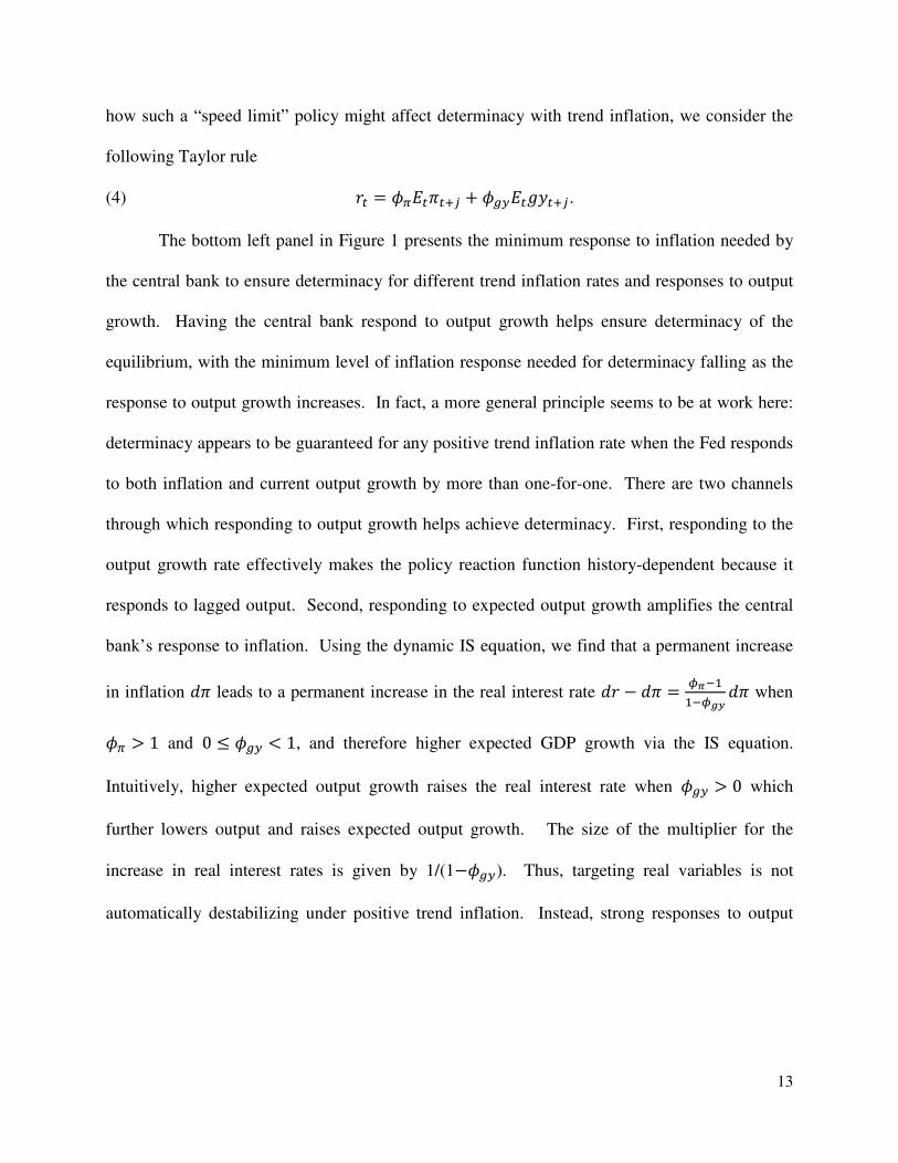
how such a “speed limit” policy might affect determinacy with trend inflation, we consider the
following Taylor rule
(4) �� = 78����� + 7CD�������.
The bottom left panel in Figure 1 presents the minimum response to inflation needed by
the central bank to ensure determinacy for different trend inflation rates and responses to output
growth. Having the central bank respond to output growth helps ensure determinacy of the
equilibrium, with the minimum level of inflation response needed for determinacy falling as the
response to output growth increases. In fact, a more general principle seems to be at work here:
determinacy appears to be guaranteed for any positive trend inflation rate when the Fed responds
to both inflation and current output growth by more than one-for-one. There are two channels
through which responding to output growth helps achieve determinacy. First, responding to the
output growth rate effectively makes the policy reaction function history-dependent because it
responds to lagged output. Second, responding to expected output growth amplifies the central
bank’s response to inflation. Using the dynamic IS equation, we find that a permanent increase
in inflation E leads to a permanent increase in the real interest rate E� − E = FG����FHI E when
78 > 1 and 0 ≤ 7CD < 1, and therefore higher expected GDP growth via the IS equation.
Intuitively, higher expected output growth raises the real interest rate when 7CD > 0 which
further lowers output and raises expected output growth. The size of the multiplier for the
increase in real interest rates is given by 1/(1−7CD). Thus, targeting real variables is not
automatically destabilizing under positive trend inflation. Instead, strong responses to output
14
growth help restore the basic Taylor principle whereas strong responses to the output gap can be
destabilizing.9
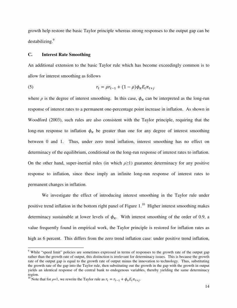
C. Interest Rate Smoothing
An additional extension to the basic Taylor rule which has become exceedingly common is to
allow for interest smoothing as follows
(5) �� = L���� + �1 − L�78�����
where ρ is the degree of interest smoothing. In this case, 78 can be interpreted as the long-run
response of interest rates to a permanent one-percentage point increase in inflation. As shown in
Woodford (2003), such rules are also consistent with the Taylor principle, requiring that the
long-run response to inflation 78 be greater than one for any degree of interest smoothing
between 0 and 1. Thus, under zero trend inflation, interest smoothing has no effect on
determinacy of the equilibrium, conditional on the long-run response of interest rates to inflation.
On the other hand, super-inertial rules (in which ρ≥1) guarantee determinacy for any positive
response to inflation, since these imply an infinite long-run response of interest rates to
permanent changes in inflation.
We investigate the effect of introducing interest smoothing in the Taylor rule under
positive trend inflation in the bottom right panel of Figure 1.10
Higher interest smoothing makes
determinacy sustainable at lower levels of 78. With interest smoothing of the order of 0.9, a
value frequently found in empirical work, the Taylor principle is restored for inflation rates as
high as 6 percent. This differs from the zero trend inflation case: under positive trend inflation,
9 While “speed limit” policies are sometimes expressed in terms of responses to the growth rate of the output gap
rather than the growth rate of output, this distinction is irrelevant for determinacy issues. This is because the growth
rate of the output gap is equal to the growth rate of output minus the innovation to technology. Thus, substituting
the growth rate of the gap into the Taylor rule, then substituting out the growth in the gap with the growth in output
yields an identical response of the central bank to endogenous variables, thereby yielding the same determinacy
region. 10
Note that for ρ=1, we rewrite the Taylor rule as �� = ���� + 78����� .

15
interest smoothing helps achieve determinacy even conditional on the long-run response to
inflation. This suggests that history-dependence is particularly useful in improving the
determinacy properties of interest rate rules when > 0. In addition, super-inertial rules (in
which ρ≥1) continue to guarantee determinacy for any positive response to the inflation rate,
exactly as was the case with = 0.
D. Price Level Targeting
Another policy approach often considered in the literature is price-level targeting (PLT). To
model this, we follow Gorodnichenko and Matthew D. Shapiro (2007) and write the Taylor rule
as
�� = 7MEN�
where dpt is the log deviation of the price level (O�) from its target path (O�∗)
EN� ≡ QRO� − QRO�∗ = SEN��� + �. The price gap depends on the lagged price gap and the current deviation of inflation from the
target. The parameter δ indicates how “strict” price-level targeting is. In the case of δ = 0, the
price-level gap is just the deviation of inflation from its target and the Taylor rule collapses to the
basic inflation targeting case. When δ=1, we have strict price level targeting in which the central
bank acts to return the price level completely back to the target level after a shock. The case of 0
< δ < 1 is “partial” price level targeting, in which the central bank forces the price level to return
only partway to the original target path. By quasi-differencing the Taylor rule after
substituting in the price gap process, one can readily show that this policy is equivalent to the
following Taylor rule:
�� = S���� + 7M� ,
16
which is observationally equivalent to the basic Taylor rule with interest smoothing. Thus, when
the central bank pursues strict PLT (δ = 1), this is equivalent to the central bank having a super-
inertial rule. Determinacy is therefore guaranteed for any positive response to the price level
(and therefore inflation). Thus, the result of Woodford (2003) that strict PLT guarantees
determinacy in a Calvo type model with zero trend inflation continues to hold (at least
numerically) under positive trend inflation. In addition, partial PLT (0<δ<1) will yield the exact
same results as interest smoothing. The stricter the PLT (the higher the δ), the smaller the long-
run response to inflation will need to be to sustain a determinate REE for positive trend levels of
inflation.
E. Positive Trend Inflation and Economic Stabilization within the Determinacy Region
While all of our results have focused on the determinacy implications of positive trend inflation,
one can also consider the effects of trend inflation on economic stabilization within the
determinacy region. Specifically, the question we want to address is how strongly the central
bank should respond to inflation under positive trend inflation to achieve the same welfare from
stabilization as under zero trend inflation. To assess the welfare gains due to stabilization
policies under zero and positive trend inflation, we derive the second order approximation to the
consumer utility function augmented with external habit formation in consumption when can
differ from zero.11,12
11
S. Boragan Aruoba and Schorfheide (2009) investigate how trend inflation affects social welfare in the steady
state. The first order effects documented in that paper are not dependent on our policy rules which are functions of
deviations of inflation, output gap or any other relevant variable from the steady state. Hence, our analysis is more
informative about the value of stabilization policies. Stephanie Schmitt-Grohé and Martin Uribe (2007) consider the
benefits of stabilization policies with positive trend inflation. However, their calibration imposes that 80 percent of
firms can reset prices every period and that the elasticity of demand is relatively low implying low strategic
complementarity. With this calibration, positive trend inflation set at low levels as calibrated in Schmitt-Grohé and
Uribe (2007) is not likely to lead to any significant departures from the standard Taylor principle, which is
consistent with our robustness analysis below. Ascari and Ropele (2007) evaluate the effects of inflation and output
gap variability given positive trend inflation. Our analysis is different in two key respects. First, they postulate a loss

17
Proposition 1: The second order approximation to consumer utility
TU��� " @� Vln 1X���Y���Z 2 − �1 + ������ [ \�]������+<;E]�
!^
∞
� !
is given by
1 − @ℎ1 − @ V�1 + ��var����
+ `a�,D� − 1
� + �1 + �� b1 + � − 1� a�,Da!,Dcd �1 − (�e� + (
1 − @( var���^
where a�,D = f1 − ;ghi<;
i jg�l f1 + ;ghi<;
i jg�lmn , a!,D = f�� h)��
) j Υ�l f1 + ;ghi<;
i jgΥ�l�n , Υ� =�varr�log ����]�/��s�� = �� �(/�1 − (��, e = (Π�θ��/�1 − (Π�θ���, h is the degree of habit
formation in consumption, and Ht is the exogenously determined (“external”) habit which is
equal to lagged consumption.
Proof: see Coibion and Gorodnichenko (2008).
It is straightforward to show that, for any plausible calibration of �, (, � and , the weight
on inflation variability increases with the level of trend inflation . Hence, the central result of
this proposition is that positive trend inflation makes stabilization (specifically with respect to
inflation) more valuable. This finding is intuitive: the level of cross-sectional price dispersion
increases with positive trend inflation and hence more variable inflation has a larger effect on
welfare.
function rather than derive it as a second order approximation to consumer utility. Second, they consider policies
under discretion or commitment while we analyze Taylor-type rules. 12
Note that technology shocks are the only economic disturbance in our model. Without habit formation, permanent
innovations to the level of technology have no effects on inflation or the output gap. We also experimented with
using specifications where there are transitory changes in technology and no habit formation and obtained
qualitatively similar results.

18
Using the second order approximation to consumer utility and the contemporaneous
Taylor rule as in equation (2), we can assess what policy response 78 is required to maintain a
fixed level of expected utility as trend inflation increases.13
Let us define 78|8�,u as the minimal
policy response necessary to achieve utility level v given trend inflation . Figure 2 shows the
ratio 78|8�,u/78|!,u for different where v is equal to the level of utility a policymaker can
achieve with the lowest 78 which yields determinacy at 6 percent trend inflation, the highest
level of trend inflation in our analysis. Irrespective of what degree of habit formation h we
choose, the policymaker must be increasingly aggressive to inflation as rises. We conclude that
the key effect of positive trend inflation on determinacy, i.e. requiring stronger responses to
inflation by the central bank, also generally applies within the parameter space in which
determinacy occurs.
III. Monetary Policy and Determinacy since the 1970s
Under positive trend inflation, the Taylor principle is no longer a sufficient condition for
determinacy, which implies that exercises focusing only on the inflation response in a Taylor
rule will in general be insufficient to answer whether this rule is consistent with a determinate
equilibrium.14
The previous section shows that one must simultaneously take into account all of
the response coefficients of the central bank’s policy function, the level of trend inflation, and
the model. In this section, we revisit the issue of how monetary policy may have changed before
and after the Volcker disinflation and whether any such changes may have moved the economy
13
When we compare utility for different levels of trend inflation, we focus only on the terms which depend on
stabilization policies. We ignore the first order effects of trend inflation on welfare because they do not depend on
stabilization policy. 14
Troy Davig and Eric M. Leeper (2007) argue that the possibility of the central banker switching to a policy rule
consistent with determinacy (good policy) can lead to determinant outcomes even during times when the central
banker’s policy rule is not sufficiently aggressive to guarantee determinacy (bad policy). In other words, the
possibility of switching to the good policy mitigates the effects of the bad policy. However, Davig and Leeper
observe that the bad policy will still lead to increased volatility of macroeconomic variables. Hence, we continue to
associate periods of bad policy with periods of increased volatility.

19
out of an indeterminate equilibrium in the pre-Volcker era in light of how determinacy results
hinge on the trend inflation rate. In section A, we estimate policy reaction functions for each
time period. In section B, we feed the estimated parameters of the policy rules into our model to
assess the determinacy implications of the differences in response coefficients across the two
periods given different trend inflation rates. Section C considers counterfactual experiments to
study which changes in the policy rule have been most important and what further changes the
Federal Reserve could pursue to strengthen the prospects of achieving determinacy. In section
D, we allow for time-varying parameters in the policy rule from which we can extract a time-
varying measure of trend inflation. By combining our implied measure of trend inflation and the
time-varying parameters of the policy rule with our model, we construct a time series of the
probability of the US economy being in a state of determinacy since the late 1960s. In section E,
we investigate the robustness of our baseline determinacy results to parameter values and
alternative price setting assumptions.
A. Estimation of the Federal Reserve’s Reaction Function
Our baseline empirical specification for the Fed’s reaction function is a generalized Taylor rule
in which we assume there is a single break in trend inflation as well as in the coefficients of the
response function around the time of the Volcker disinflation. Our baseline period-specific
estimated Taylor rule is thus
(6) �� = w + �1 − L� − L���78����� + 7CD������� + 7:������� + L����� + L����� + 3�,
where 3� is an error term. This specification allows for interest smoothing of order two, as well
as a response to inflation, output growth, and the output gap. Allowing for responses to both the
output gap and output growth is necessary because the two have different implications for

20
determinacy with positive trend inflation.15
The constant term c consists of the steady-state level
of the interest rate, plus the (constant) level of trend inflation, as well as the target levels of
output growth and output gap. To estimate equation (6), we follow Orphanides (2004) and use
real-time data for the estimation. Specifically, we use the Greenbook forecasts of current and
future macroeconomic variables prepared by staff members of the Fed a few days before each
FOMC meeting. The interest rate is the target federal funds rate set at each meeting, from
Christina D. Romer and David H. Romer (2004). The measure of the output gap is based on
Greenbook forecasts, as compiled by Orphanides (2003, 2004). Data are available from 1969 to
2002 for each official meeting of the FOMC. We consider two time samples: 1969-1978 and
1983-2002. We drop the period from 1979 to 1982 in which the Federal Reserve officially
abandoned interest rate targeting in favor of targeting monetary aggregates. Each t is a meeting
of the FOMC. From 1969-1978, meetings were monthly, whereas from 1983 on, meetings were
held every 6 weeks. Note that this implies that the interest smoothing parameters in the Taylor
rule are not directly comparable across the two time periods.16
Table 1 presents results of the least squares estimation of equation (6) over each time
period for three cases: contemporaneous Taylor rule, forward-looking Taylor rule, and mixed.17
15
We show in Coibion and Gorodnichenko (2008) that allowing for PLT yields similar conclusions as specifications
without. 16
John Cochrane (2007) argues that the central bank’s response to inflation will be unidentified in New Keynesian
models when the Taylor rule includes a stochastic intercept term that corresponds to the natural rate of interest, i.e.
the rate of interest that would hold in the frictionless economy. However, Eric Sims (2008) shows that Cochrane’s
argument holds only if the central bank is responding one-for-one to fluctuations in the natural rate of interest, an
unlikely scenario due to the inherent difficulty in measuring the natural rate of interest, particularly in real time.
More generally, the Fed may be stabilizing inflation with off-equilibrium path threats that may not be observed in
equilibrium. However, in practice, periods of apparent indeterminacy in the policy rule have come when trend
inflation is high. Thus it is highly unlikely that the Fed has effectively been using off-equilibrium strategies over this
period to stabilize inflation. 17
We think there are several reasons why estimation by least squares (LS) is likely to be adequate. First, Hausman
tests indicate that instrumental variable estimation leads to same results as LS, which indicates the exogeneity
assumption is likely to be satisfied. Second, if Greenbook forecasts were made under assumptions about future
policy actions that were systematically overturned, then these forecasts would be inferior to those made by agents
who made better projections of future policy actions, such as professional forecasters. Yet Romer and Romer (2000)
document that Greenbook forecasts of inflation systematically outperform professional forecasters. Third, we can

21
In the case of the contemporaneous Taylor rule, we use the central bank’s forecast of values for
the current quarter. In the case of the forward-looking rule, we use the forecast of the average
value over the next two quarters (but three quarter ahead forecast for the output gap). We find
that interest rate decisions are best modeled (in terms of fitting the data) as a function of
forecasts of future inflation but forecasts of the contemporaneous output gap and output growth
rate.18
We will treat this specification as the baseline in subsequent sections. In addition to point
estimates, standard errors and selected statistics of fit, we report the sum of the interest
smoothing parameters converted to a quarterly frequency.19 We also include the probability
value of the null that each of the parameters and the sum of interest smoothing parameters are the
same in the two periods.
We find that the Fed’s response to inflation in the pre-Volcker era satisfied the Taylor
principle in forward-looking specifications, but not under the contemporaneous Taylor rule.
Because the forward-looking specification is statistically preferred to a contemporaneous
response to inflation, our evidence supports the argument of Orphanides (2004) that the Fed
satisfied the Taylor principle in both periods, albeit weakly so. Like Orphanides, we also find
that while our estimates consistently point to a stronger response by the Fed to inflation in the
latter period, we can only reject the null of no change in the response to inflation in the case of
the mixed rule. Thus, our estimates of the Fed’s response coefficients do not provide strong
augment the right-hand-side of equation (6) with a direct measure of monetary policy innovations from Refet
Gürkaynak, Brian Sack and Eric Swanson (2005), who identify monetary policy innovations by comparing Fed
Funds Futures markets predictions of FOMC decisions with actual decisions. Adding this variable eliminates the
omitted variable bias and hence LS are consistent. We found that estimates in this augmented specification are
remarkably close to the specification without policy shocks identified via Fed Funds Futures. Details are available
in Coibion and Gorodnichenko (2008). 18
Specifically, we consider all possible variants of forward-looking and contemporaneous-looking choices for
inflation, output gap, and output growth responses and use the AIC to select the best specification. 19
Because there is no convenient formula for converting AR(2) parameters from monthly or 6-weekly frequency to
quarterly, we use the following approach: given estimated AR(2) parameters, we simulate an AR(2) process at the
original frequency, and then create a new (average) series at the quarterly frequency. We then regress the quarterly
series on two lags of itself over a sample of 50,000 periods and report the sum of the estimated parameters.

22
support for the claims of Taylor (1999) and Clarida et al (2000) that the failure to satisfy the
basic Taylor principle before Volcker placed the US economy in an indeterminate region.
However, we do find that other response coefficients have changed in statistically significant
ways. First, interest rate decisions have become more persistent, in the sense that the sum of the
autoregressive components is higher in the latter period than in the early period, and statistically
significantly so in two out of three specifications. Second, the Federal Reserve has changed how
it responds to the real side of the economy. Whereas the period before the Volcker disinflation
was characterized by a strong long-run response to the output gap, but no statistically discernible
response to output growth, the period since the Volcker disinflation displays much stronger long-
run responses by the Fed to output growth than to the output gap. Interestingly, all of the policy
changes made by the Fed since the Volcker disinflation—stronger response to output growth and
inflation, more interest smoothing, and weaker response to output gap (albeit not statistically
significantly so for the latter)—will tend to make determinacy more likely.
B. Determinacy Before and After the Volcker Disinflation
To assess the implications of our estimated response functions, we feed the estimated parameters
from each Taylor rule into the model described and calibrated in section I.B to examine the
determinacy implications of monetary policy over the two samples. We first consider whether
the model yields a determinate rational expectations equilibrium (REE) given the estimated
parameters of the Taylor rule for two trend inflation rates – 3 percent and 6 percent – designed to
replicate average inflation rates in each of the two time periods. In addition, we consider how
determinacy varies over the statistical distribution of our parameter estimates. For each type of
Taylor rule and each sample period, we draw 10,000 times from the distribution of the estimated
parameters and assess the fraction of draws that yield a determinate rational expectations

23
equilibrium at 3 percent and 6 percent trend inflation. The results are presented in the bottom
panel of Table 1.20
First, we find that the pre-1979 response of the central bank implied an indeterminate
REE given the average inflation rate of that time (6 percent). This is a very robust implication of
the Taylor rule estimates: both the contemporaneous and mixed Taylor rules yield zero percent
of draws consistent with determinacy while the forward-looking rule delivers a probability of
determinacy of only 12 percent, despite a point estimate of 1.75 for the Fed’s response to
expected inflation. On the other hand, the post-1982 response is consistent with a determinate
REE at the low average inflation rate of this period (3 percent). Using our preferred
specification, the mixed Taylor rule, more than 99 percent of the empirical distribution of
parameters yields determinacy. Thus, like Taylor (1999), Clarida et al (2000) and others, we
find that monetary policy before Volcker led to indeterminacy in the 1970s, but that since 1982
the Fed’s response has helped ensure determinacy.
Our approach also allows us to assess the relative importance of the change in the Fed’s
response function versus the change in trend inflation for altering the determinacy status of the
economy. For example, had the Fed maintained its pre-1979 response function but lowered
average inflation from 6 percent to 3 percent per year (via a change in the inflation target in the
Taylor rule), the US economy would have remained in the indeterminacy region of the parameter
space. Thus, the Volcker disinflation, during which average inflation was brought down, would
have been insufficient to guarantee determinacy without a change in the Fed’s response function
as well. Similarly, we also find that the Fed’s response to macroeconomic variables since 1982,
20
Before feeding estimated parameters into the model, we first convert the interest smoothing parameter into a
quarterly frequency and divide the coefficient on the output gap by four, since the Taylor rules are estimated using
annualized rates, the Taylor rule in the model is written in terms of quarterly rates, and the output gap is scale
invariant.

24
while consistent with determinacy at 3 percent trend inflation, is only marginally consistent with
determinacy at the inflation rate of the 1970s, with only sixty percent of draws from the
distribution of estimated parameters from the mixed Taylor rule predicting determinacy at this
inflation rate. Thus, the estimated parameters are near the edge of the parameter space consistent
with a unique REE. This implies that if the Fed in the 1970s had simply switched to the current
policy rule without simultaneously engaging in the Volcker disinflation, it is quite possible that
the US economy would have remained subject to self-fulfilling expectations-driven fluctuations.
The shift from indeterminacy to determinacy thus appears to have been due to two major policy
changes: a change in the policy rule and a decline in the inflation target of the Federal Reserve
during the Volcker disinflation.
C. Counterfactual Experiments
In this section, we perform counterfactual experiments designed to isolate the contribution of
each policy change for determinacy, the results of which are presented in Table 2. Consider first
the effect of switching the Fed’s response to inflation 78 across the two time periods. For the
pre-1979 period at 6 percent trend inflation, this has no effect on determinacy, meaning that the
fraction of draws from the empirical distribution of parameter estimates yielding a determinate
REE is essentially unchanged at 0 percent. This means that if the only policy change enacted by
the Fed had been to raise its response to inflation to the post-1982 level, but leaving its other
response coefficients and the trend inflation unchanged, the US economy would have remained
in an indeterminate equilibrium. Thus, while our findings support the argument of Clarida et al
(2000) that the US moved from indeterminacy to determinacy during the Volcker disinflation,
we emphasize not just the change in the Fed’s response to inflation, which by itself was not
enough to shift the US economy out of the indeterminacy of the 1970s, but rather that this policy

25
change combined with the Volcker disinflation can account for much of the movement away
from indeterminacy. Specifically, we find that if the Fed had maintained its pre-Volcker policy
rule but used the post-1982 inflation response, then this single policy switch combined with the
Volcker disinflation would have raised the likelihood of determinacy to about two-thirds.
We also consider the implication of switching the degree of interest smoothing across
periods and the response to output growth, both of which are statistically different in the two
time periods (see Table 1). For interest smoothing, we find almost identical results as in the
baseline case, indicating that the increased inertia of interest rate decisions since the Volcker
disinflation cannot account for the change in determinacy across periods. Switching the response
to output growth across the two periods has a more important effect. If we start with the
estimated post-1982 policy reaction function and switch 7CD to its pre-1979 value, the fraction of
draws yielding determinacy in the post-1982 period at 3 percent (6 percent) trend inflation would
have been only 91 percent (26 percent) instead of 99 percent (62 percent). On the other hand,
starting from the pre-1979 policy rule and raising 7CD, to the post-1982 level has almost no
effect on determinacy. This indicates that the change in 7CD complemented the other policy
changes in terms of restoring determinacy, but could not, by itself, account for the reversal in
determinacy around the time of the Volcker disinflation.
Finally, we consider the effect of the decrease in the Fed’s response to the output gap, a
policy difference strongly emphasized by Orphanides (2004), although we cannot reject the null
of no change in the Fed’s response to the gap across time periods. We find that if the post-1982
Fed had responded as strongly to the output gap as they did before Volcker, then the likelihood
of the US economy being in the indeterminacy region would be somewhat higher, particularly at
higher rates of inflation. At 6 percent trend inflation, the fraction of draws yielding determinacy
26
falls from 62 percent to 33 percent. Thus, this result supports the emphasis placed by
Orphanides (2004) on the lower response to the output gap by the Fed since the Volcker era, but
for a different reason. Orphanides stresses that if the output gap is mismeasured in real-time,
then a strong response to the output gap, like that followed by the Fed in the 1970s, can be
destabilizing. Our interpretation is instead that even if the output gap is perfectly measured by
the central bank, strong responses to the output gap can be destabilizing by raising the
probability of indeterminacy.
We can extend our analysis by investigating how the central bank can further minimize
the likelihood of indeterminacy. Thus, we consider determinacy prospects using each policy rule
but imposing 7: = 0.21
In the post-1982 period, eliminating the response to the output gap
would raise the likelihood of determinacy significantly. This is most clearly visible at the 6
percent inflation rate, when eliminating the Fed’s response to the output gap would raise the
probability of determinacy from 62 to 99 percent. Thus, while the Fed has improved
determinacy prospects somewhat by reducing its response to the output gap since the 1970s, a
complete elimination of this response would be better yet. Importantly, this does not imply that
the Federal Reserve is best served by not responding to the real side of the economy. Consider
the counterfactual of no response by the Fed to both the output gap and output growth in each
time period. In the post-1982 period, the prospects for determinacy are lower than in the case
with just zero response to the output gap, particularly at higher inflation rates. For the latter,
eliminating any response to the real side of the economy yields determinacy in less than 13
percent of draws, instead of the 99 percent when only the response to the output gap is
eliminated. Thus, the current strong response to output growth by the Federal Reserve is well-
21
Here, we draw from each period’s distribution of parameters, then impose that the relevant coefficient be exactly
zero for each draw.
27
justified, and would play an important stabilizing role were the Fed to completely eliminate
responding to the output gap. Furthermore, a positive response to the real side of the economy
should not necessarily be interpreted as central bankers being “dovish” on inflation.
D. Time-Varying Trend Inflation
Our baseline estimation approach assumes that trend inflation, as well as the central bank’s target
for real GDP growth and the output gap, is constant within each time period. In this section, we
relax these assumptions and extract a measure of trend inflation which allows us to construct a
time series for the probability of determinacy for the U.S. economy. Our approach follows
Boivin (2006), who estimates a similar Taylor rule with time-varying coefficients. We
generalize the Taylor rule in equation (6) to:
�� = � + x� + #1 − L�,� − L�,�$%78,�#����� − �$ + 7CD,�#������� − �� � $+ 7:,�#������ − �y�$& + L�,������ − � − x�� + L�,������ − � − x�� + 3�
where � is the target rate of inflation, x� is the equilibrium real interest rate, �� � is the target
rate of growth of real GDP, and �y� is the target level of the output gap. We can rewrite this as
(7) �� = w� + #1 − L�,� − L�,�$�78,������ + 7CD,�������� + 7:,��������
+ L�,����� + L�,����� + 3�
where the time-varying constant term is given by
(8) w� = #1 − L�,� − L�,�$%#1 − 78,�$ � + x� − 7CD,��� � − 7:,��y�&.
To estimate the parameters of equation (7), we follow Boivin (2006) and assume that each of the
parameters follows a random walk process and allow for two breaks in the volatility of shocks to
the parameters: 1979 and 1982. Using the Kalman filter and the corresponding smoother, we
construct time series of the response coefficients of the Taylor rule and of the time-varying
constant.

28
The results for the estimated parameters, including the time-varying constant, are
presented in Figure 3, along with one standard deviation confidence intervals. The results
broadly confirm those in the baseline estimation: namely, there was a sharp increase in the Fed’s
response to inflation and output growth around the time of the Volcker disinflation, as well as a
rise in the degree of interest smoothing, and there was little change in the response to the output
gap once one allows for time-varying parameters. In addition, the time-varying parameters allow
us to paint a more nuanced picture of monetary policy in the pre-Volcker era. Specifically, the
estimated coefficients in 1969 are remarkably similar to those for the 1990s with strong
responses to output growth and inflation, but there was a discernible change in the Fed’s
response function in the early 1970s that was reversed during the Volcker disinflation.
To extract a measure of trend inflation from the time-varying constant, we make
additional assumptions about the equilibrium real interest rate and the Fed’s targets for real GDP
growth and the output gap. We follow Sharon Kozicki and Peter A. Tinsley (2009) and
approximate the equilibrium real interest rate, the target growth rate of real GDP, and the target
output gap by using the Hodrick-Prescott filter over each time period to extract a trend measure
of each series, which we then feed into equation (8), along with estimates of time-varying
parameters, to extract our measure of trend inflation. The bottom right panel of Figure 3 presents
our (smoothed) estimate of the latter, along with one standard deviation confidence intervals.
This measure of time-varying trend inflation paints a similar picture of changes in monetary
policy as the response coefficients. Namely, at the start of the sample, the Fed’s target rate of
inflation was low, around 3 percent, and rose slightly over the early 1970’s. Starting around
1975, we see a substantial increase in the Fed’s target inflation, which peaks at approximately 8
percent in 1978. Thus, the data point to increasing accommodation of inflationary pressures by
the Federal Reserve in the mid to late 1970s. The latter is reversed during the Volcker

29
disinflation, after which target inflation is progressively reduced to 2 percent by the early 2000’s.
This behavior of trend inflation is remarkably consistent with the estimates of Cogley et al
(forthcoming) and Ireland (2007) despite the differences in approaches.
Given the estimated time series of the Fed’s response coefficients and our measure of
trend inflation, we can construct a time series of the probability of determinacy for the U.S.
economy given the estimated distribution of parameters in the Taylor rule (7). We do this under
three alternative assumptions. The first is to allow for time-varying response coefficients but
impose a constant rate of 3 percent trend inflation. The second is identical except that we impose
a constant rate of 6 percent trend inflation. The third approach again uses time-varying response
coefficients but also makes use of our time-varying estimate of trend inflation. The results are
presented in Figure 4. Looking first at the estimates using time-varying trend inflation, the
results from our baseline estimation are re-confirmed: the U.S. economy was very likely in a
state of indeterminacy before the Volcker disinflation but not thereafter. Again, the use of time-
varying parameters provides a more detailed perspective on the pre-Volcker era. At the start of
our sample period, the probability of determinacy was close to one, reflecting the low estimate of
trend inflation at the time as well as the strong responses to inflation and output growth.
However, we can observe a rapid deterioration in the stabilization properties of monetary policy
in the early 1970s such that by 1975 the probability of the U.S. economy being in a state of
determinacy was less than ten percent. This was not reversed until the Volcker disinflation,
since which the probability of determinacy has exceeded eighty percent. This finding is
consistent with the view laid out in Romer and Romer (2002) emphasizing that good policy
prevailed during Martin’s chairmanship of the Fed (which ended in 1970) and returned with
Volcker’s ascent.

30
The results with time-varying parameters also confirm the key role played by changes in
the level of trend inflation in accounting for the apparent transition from determinacy to
indeterminacy in the early 1970s and then back to determinacy during the Volcker disinflation.
Consider the first transition in the early 1970s. Our estimates imply that if the Fed had only
changed the coefficients of its response function but held the target rate of inflation constant at 3
percent, the economy would have been right at the edge of the indeterminacy region, implying
that the change in trend inflation accounts for approximately half of the switch from determinacy
to indeterminacy over this time period. After the Volcker disinflation, the results are similar: had
the Fed only changed its response coefficients but left its target inflation in the neighborhood of
six percent, the probability of indeterminacy would still have been around fifty percent by the
mid-1990s rather than ten percent. Thus, these results reinforce the key point that one cannot
address determinacy issues only by focusing on the response coefficients of the central bank,
instead we need to consider the interaction of the central bank’s reaction function with trend
inflation.
E. Robustness Analysis
The fact that higher trend inflation raises the likelihood of indeterminacy reflects the increased
importance of forward-looking behavior in firms’ price setting decisions. Specifically, when
firms reset prices in the Calvo model, the weight placed on future profits depends strongly on
how likely a firm is to not have altered its price by that period. Thus, greater price stickiness will
naturally increase the sensitivity of reset prices to expectations of future macroeconomic
variables. As a result, one would expect indeterminacy to become increasingly difficult to
eliminate as the degree of price rigidity rises.
31
To see whether this is indeed the case, we consider two alternative degrees of price
stickiness. First, we follow Bils and Klenow (2004) who find that firms update prices every 4 to
5 months on average which corresponds to (=0.40 in our model. Second, we follow Nakamura
and Steinsson (2008) who find much longer durations of price spells ranging between 8 and 11
months on average. In this case, we set (=0.70. We reproduce the determinacy results of
section B. in Table 3 using the mixed Taylor rule for each time period. Under the Bils and
Klenow case, we recover our baseline results of indeterminacy in the 1970s but determinacy
after the Volcker disinflation. However, we can see that determinacy is more easily sustained
under lower levels of price rigidity by the fact that the fraction of the empirical distribution
yielding determinacy is consistently higher than in the baseline case. In addition, using this
lower rate of price-stickiness implies that determinacy would have been achieved solely through
the change in the Fed’s response to macroeconomic variables. Using the degree of price
stickiness from Nakamura and Steinsson moves all of the quantitative results in the opposite
direction. For the pre-Volcker era, the results are qualitatively similar to our baseline findings,
with indeterminacy occurring consistently at both inflation rates. However, with this higher
degree of price stickiness, we now find that the current policy rule is likely inconsistent with
determinacy: even at 3 percent inflation, less than 50 percent of the empirical distribution of
Taylor rule estimates yields a determinate REE.
Clearly, the degree of price stickiness plays an important role in determinacy conditions.
However, the importance of this variable is likely overestimated under Calvo pricing. This setup
forces firms to place some weight on possible future outcomes in which their relative price
would be so unprofitable that “real world” firms would likely choose to pay a menu cost and
32
reset their price.22
An alternative approach to Calvo pricing is the staggered contracts approach
of Taylor (1977) in which firms set prices for a pre-determined duration of time. This pricing
assumption can loosely be thought of as a lower bound on forward-looking behavior (conditional
on price durations) since it imposes zero weight on expected profits beyond those of the contract
length in the firm’s reset price optimization. We replicate our results using staggered pricing
with firms setting prices for three quarters and display the results in Table 3. For the pre-Volcker
era, the results again largely point to indeterminacy at high levels of inflation. However, the
post-1982 policy rule is now consistent with determinacy at both 3 percent and 6 percent
inflation rates. In fact, the results using staggered price setting with duration of 9 months are
very close to those using Calvo price setting with average price duration of 5 months. We
interpret Taylor pricing as setting a lower bound on determinacy issues (conditional on average
price durations) and Calvo pricing an upper bound. Despite the sensitivity of determinacy results
to these variations, what seems clear is that the U.S. economy was in an indeterminate region of
the parameter space in the pre-Volcker era given the high average inflation of that time, but
moved into the determinacy region after 1982. The relative importance of the decrease in trend
inflation versus the changes in the Fed’s response to macroeconomic conditions, on the other
hand, is somewhat sensitive to the price-setting model and average price durations used.
A closely related issue is how to model price adjustment frictions faced by firms. A
common extension is to model firms as facing sticky prices with indexation, i.e. allowing non-
reoptimizing firms to automatically adjust their prices by some fraction of either last period’s
inflation or the trend inflation rate, thereby increasing the persistence of the inflation process (see
22
Another way to see this limitation of the Calvo model is to note that using Nakamura and Steinsson rates of price-
setting, the Calvo model breaks down (i.e. γ2 ≥ 1) at an inflation rate of 6.1 percent.

33
Tack Yun (1996) and Lawrence Christiano et al (2005)).23
Ascari and Ropele (2009) have
shown that allowing for indexation diminishes the determinacy issues that arise with positive
trend inflation. The reason is that indexation decreases the devaluation of firms’ reset prices that
comes from positive trend inflation. In the special case of full indexation—firms raise their price
fully with past inflation or the level of trend inflation—determinacy in the model becomes
completely insensitive to trend inflation. We follow Yun (1996) and consider the case in which
firms index their prices to trend inflation by some fraction ω, where 0 ≤ x ≤ 1. We replicate our baseline empirical results on determinacy prospects based on our mixed
Taylor rule estimates for each time period and for different levels of price indexation in Figure
5.24
Figure 5 makes clear that as indexation rises, the fraction of the empirical distribution of
Taylor rule estimates consistent with determinacy also rises. Note that it takes fairly high levels
of indexation to change our results substantially. For example, for the probability of determinacy
to exceed 50 percent in the pre-1979 era at 6 percent inflation requires price indexation of more
than 0.9. Thus, the result that the US economy was likely in an indeterminacy region pre-
Volcker but not thereafter is robust to substantial levels of price indexation. However, the
importance of taking into account positive trend inflation to reach this conclusion is also clearly
illustrated in Figure 5. This can be seen by examining the results with full price indexation (ω =
1), in which case the supply-side of the model is observationally equivalent to the NKPC with
23
Our baseline model does not include this feature for three reasons. First, the workhorse New Keynesian model is
based only on price stickiness, making this the most natural benchmark for our analysis (Clarida et al (1999) and
Michael Woodford (2003)). Second, any price indexation implies that firms are constantly changing prices, a
feature strongly at odds with the empirical findings of Bils and Klenow (2004) and more recently Nakamura and
Steinsson (2008), among many others. Third, while indexation is often included to replicate the apparent role for
lagged inflation in empirical estimates of the NKPC (see Jordi Gali and Mark Gertler 1999), Cogley and Sbordone
(2008) find no evidence of indexation after controlling for trend inflation. 24
We continue to assume λ=0.55, although another drawback of introducing indexation into a model is that it is
unclear how to link price stickiness from the micro data to price setting models with indexation in which firms are
continuously changing prices.
34
zero trend inflation.25
Determinacy is then driven almost exclusively by the Fed’s response to
inflation, yielding a probability of determinacy of more than 99 percent in the post-1982 era and
approximately 55 percent in the pre-1979 era. The latter number reflects the fact that the point
estimate of the Fed’s long-run response to inflation is barely above one, so slightly more than
half the draws from the empirical distribution will satisfy the Taylor principle and generate
determinacy.
An important parameter in New Keynesian models is the elasticity of substitution θ
which affects the degree of strategic complementarity in price setting As a robustness check, we
consider the much lower value of θ=6, which implies markups of 20 percent. With a lower
elasticity of substitution, strategic complementarity in price setting is substantially reduced so
that firms focus less on the pricing behavior of other firms and hence on trend inflation.
Correspondingly, a lower θ tends to offset some of the effects of positive trend inflation on
determinacy. As shown in Table 3, this does not alter our baseline result of indeterminacy in the
1970s switching to determinacy in the 1980s, but it does reduce the quantitative importance of
trend inflation in accounting for the results, which is similar to our findings for reduced price
stickiness as in Bils and Klenow (2004). However, with lower levels of strategic
complementarity, one needs longer durations of price spells to match the persistence of
macroeconomic data. We find that combinations of higher price stickiness (such as Nakamura
and Steinsson values) with lower estimates of the elasticity of substitution yield essentially the
same results as our baseline.26
25
This is why, for each time period, the 3 percent and 6 percent lines converge to the same value when ω = 1. 26
We provide additional robustness checks in Coibion and Gorodnichenko (2008).

35
IV. Conclusion
This paper sheds new light on the sources of the significant decrease in macroeconomic volatility
since the early 1980s commonly referred to as the Great Moderation. We confirm the original
insight of Clarida et al (2000) that the US economy moved from the indeterminacy region in the
1970s to determinacy since the early 1980s because of changes in monetary policy. Building on
recent work showing that the Taylor principle does not guarantee determinacy when trend
inflation is positive, we argue that despite substantial uncertainty about whether the Taylor
principle was satisfied in the pre-Volcker era, the US economy was very likely subject to sunspot
fluctuations in the 1970s given the high average rate of inflation over this time period, as well as
the Fed’s response to both inflation and the real side of the economy.
Our basic findings thus provide additional support for the well-known view that monetary
policy changes have likely played an important element in accounting for the Great Moderation.
However, the specific policy changes that we emphasize differ from the consensus monetary
policy interpretation. One novel finding is that the Volcker disinflation very likely played a key
role in restoring macroeconomic stability through its effect on the level of trend inflation. We
also show using time-varying estimates of trend inflation that the increase in the Fed’s target rate
of inflation in the early 1970s contributed to the US economy moving into the indeterminacy
region over this time period. Thus, our results strongly support studying the determinants of
trend inflation, as in Primiceri (2006), Cogley et al (forthcoming) and Ireland (2007), and
complement the recent finding, e.g. Cogley and Sbordone (2008), that accounting for trend
inflation has important effects on estimates of the New Keynesian Phillips Curve.
In addition, while most research has emphasized the central bank’s response to inflation
as the key factor for determinacy, our results move the Fed’s response to the real side of the
economy to center stage, particularly when trend inflation is relatively high. In such a setting,

36
responding to the output gap, even if perfectly measured, can be destabilizing, while responding
to output growth is stabilizing. As a result, the substantial increase in the Federal Reserve’s
response to output growth since the Volcker disinflation has played a non-negligible role in
restoring determinacy for the US economy. Our counterfactuals imply that if the Fed were to
eliminate any response to the output gap, while maintaining a strong response to output growth,
it could further improve determinacy prospects even at high (for the US) trend inflation rates.
Furthermore, we show that with positive trend inflation policymakers should respond more
aggressively to inflation to maintain a stable level of welfare even when the economy stays
inside the determinacy region.
Our analysis also has implications for ongoing events in the U.S. economy. For example,
some commentators have suggested that the severity of the current recession (which started in
the fourth quarter of 2007) marks the end of the Great Moderation. However, every recession in
the post-Volcker period has led to short-tem increases in volatility which subsequently reverted
to lower levels as the economy recovered. The current recession is following a similar, albeit
more pronounced, pattern, and volatility levels remain far below those of the 1970s. This is
consistent with our understanding of the Great Moderation as a phenomenon determined to a
significant extent by improved policy rather than luck. Indeed, the Fed’s rapid response to the
sharp contraction in the growth rate of output and its commitment to low trend inflation suggest
that volatility is likely to return to low levels as the economy recovers. Furthermore, our results
call for caution in evaluating recent arguments in favor of raising trend inflation to avoid hitting
the zero bound on interest rates in the future, since such a policy action could precipitate a return
to the volatility of the 1970s. However, further research is needed to fully understand and
quantify the implications of positive trend inflation for macroeconomic dynamics in empirical
and theoretical models as well as for normative analyses.

37
References
Aruoba, S. Boragan, and Frank Schorfheide. 2009. “Sticky Prices versus Monetary Frictions: An
Estimation of Policy Trade-offs.” National Bureau of Economic Research Working Paper
14870.
Ascari, Guido, and Tiziano Ropele. 2009. “Trend Inflation, Taylor Principle, and
Indeterminacy.” Journal of Money, Credit and Banking, 48(1): 1557-1584.
Ascari, Guido, and Tiziano Ropele. 2007. “Optimal Monetary Policy under Low Trend
Inflation.” Journal of Monetary Economics, 54(8): 2568–2583.
Basu, Susanto, and John G. Fernald, 1997. “Returns to Scale in U.S. Production: Estimates and
Implications.” Journal of Political Economy, 105(2): 249-283.
Bils, Mark, and Peter J. Klenow, 2004. “Some Evidence on the Importance of Sticky Prices.”
Journal of Political Economy, 112(5): 947-985.
Boivin, Jean, and Marc Giannoni. 2006. “Has Monetary Policy Become More Effective?”
Review of Economics and Statistics, 88(3): 445-462.
Boivin, Jean. 2006. “Has U.S. Monetary Policy Changed? Evidence from Drifting Coefficients
and Real-Time Data.” Journal of Money, Credit and Banking, 38(5): 1149-1173.
Burnside, Craig. 1996. “Production Function Regressions, Returns to Scale, and Externalities.”
Journal of Monetary Economics, 37(2): 177-201.
Calvo, Guillermo. 1983. “Staggered Prices in a Utility-Maximizing Framework.” Journal of
Monetary Economics, 12(3): 383-98.

38
Christiano, Lawrence, Martin Eichenbaum, and Charles Evans. 2005. “Nominal Rigidities and
the Dynamic Effects of a Shock to Monetary Policy.” Journal of Political Economy,
113(1): 1-45.
Clarida, Richard, Jordi Galí, and Mark Gertler. 1999. “The Science of Monetary Policy: A New
Keynesian Perspective.” Journal of Economic Literature, 37(4): 1661-1707.
Clarida, Richard, Jordi Galí, and Mark Gertler. 2000. “Monetary Policy Rules and
Macroeconomic Stability: Evidence and Some Theory.” Quarterly Journal of Economics,
115(1): 147-180.
Cochrane, John. 2007. “Identification with Taylor Rules: A Critical Review.”
http://faculty.chicagobooth.edu/john.cochrane/research/Papers/identification_taylor_rule.
pdf.
Cogley, Timothy, and Argia Sbordone. 2008. “Trend Inflation, Indexation and Inflation
Persistence in the New Keynesian Phillips Curve.” American Economic Review, 98(5):
2101–2026.
Cogley, Timothy, Giorgio E. Primiceri, and Thomas J. Sargent. Forthcoming. “Inflation-Gap
Persistence in the U.S.” American Economic Journal: Macroeconomics.
Coibion, Olivier, and Yuriy Gorodnichenko. 2008. “Monetary Policy, Trend Inflation and the
Great Moderation: An Alternative Interpretation.” National Bureau of Economic
Research Working Paper 14621.
Davig, Troy, and Eric M. Leeper. 2007. “Generalizing the Taylor Principle.” American
Economic Review, 97(3): 607-635.
Gali, Jordi, and Mark Gertler. 1999. “Inflation Dynamics: A Structural Econometric Analysis.”
Journal of Monetary Economics, 44(2): 195–222.

39
Gorodnichenko, Yuriy, and Matthew D. Shapiro. 2007. “Monetary Policy When Potential Output
Is Uncertain: Understanding the Growth Gamble of the 1990s.” Journal of Monetary
Economics, 54(4): 1132-1162.
Gürkaynak, Refet, Brian Sack, and Eric T. Swanson. 2005. “Do Actions Speak Louder Than
Words? The Response of Asset Prices to Monetary Policy Actions and Statements.”
International Journal of Central Banking, 1(1): 55-93.
Hornstein Andreas, and Alexander L. Wolman. 2005. “Trend Inflation, Firm-Specific Capital,
and Sticky Prices.” Federal Reserve Bank of Richmond Economic Quarterly, 91(4): 57-
83.
Ireland, Peter. 2004. “Technology Shocks in the New Keynesian Model.” Review of Economics
and Statistics, 86(4): 923-936.
Ireland, Peter. 2007. “Changes in the Federal Reserve’s Inflation Target: Causes and
Consequences.” Journal of Money, Credit, and Banking, 39(8): 1851-1882.
Justiniano, Alejandro, and Giorgio E. Primiceri. 2008. “The Time-Varying Volatility of
Macroeconomic Fluctuations.” American Economic Review, 98(3): 604-641.
Kahn, James A., Margaret M. McConnell, and Gabriel Perez-Quirós. 2002. “On the Causes of
the Increased Stability of the U.S. Economy.” Economic Policy Review of the Federal
Reserve Bank of New York, 8(1): 183-206.
Kiley, Michael E. 2007. “Is Moderate-to-High Inflation Inherently Unstable?” International
Journal of Central Banking, 3(2): 173-201.
Kozicki, Sharon, and Peter A. Tinsley. 2009. “Perhaps the 1970s FOMC Did What It Said It
Did.” Journal of Monetary Economics, 56(6): 842-855.
Lubik, Thomas A., and Frank Schorfheide. 2004. “Testing for Indeterminacy: An Application to
U.S. Monetary Policy.” American Economic Review, 94(1): 190-217.

40
McConnell, Margaret, and Gabriel Perez-Quirós. 2000. “Output Fluctuations in the United
States: What Has Changed since the Early 1980s?” American Economic Review, 90(5):
1464-76.
Nakamura, Emi, and Jón Steinsson. 2008. “Five Facts About Prices: A Reevaluation of Menu
Cost Models.” Quarterly Journal of Economics, 123(4): 1415-1464.
Orphanides, Athanasios, and John C. Williams. 2006. “Monetary Policy with Imperfect
Knowledge.” Journal of the European Economic Association, 4(2-3): 366-375.
Orphanides, Athanasios. 2001. “Monetary Policy Rules Based on Real-Time Data.” American
Economic Review, 91(4): 964-985.
Orphanides, Athanasios. 2002. “Monetary Policy Rules and the Great Inflation.” American
Economic Review Papers and Proceedings, 92(2): 115-120.
Orphanides, Athanasios. 2003. “Historical Monetary Policy Analysis and the Taylor Rule.”
Journal of Monetary Economics, 50(5): 983-1022.
Orphanides, Athanasios. 2004. “Monetary Policy Rules, Macroeconomic Stability and Inflation:
A View from the Trenches.” Journal of Money, Credit, and Banking, 36(2): 151-175.
Primiceri, Giorgio E. 2006. “Why Inflation Rose and Fell: Policymakers’ Beliefs and US
Postwar Stabilization Policy.” Quarterly Journal of Economics, 121(3): 867-901.
Romer, Christina D., and David H. Romer. 2000. “Federal Reserve Information and the Behavior
of Interest Rates.” American Economic Review, 90(3): 429- 457.
Romer, Christina D., and David H. Romer. 2002. “A Rehabilitation of Monetary Policy in the
1950's.” American Economic Review, 92(2): 121-127.
Romer, Christina D., and David H. Romer. 2004. “A New Measure of Monetary Shocks:
Derivation and Implications.” American Economic Review, 94(4): 1055-1084.

41
Sargent, Thomas J. 1999. The Conquest of American Inflation, Princeton University Press,
Princeton N.J.
Schmitt-Grohé, Stephanie, and Martín Uribe. 2007. “Optimal Simple and Implementable
Monetary and Fiscal Rules.” Journal of Monetary Economics, 54(6): 1702-1725.
Sims, Eric. 2008. “Identification and Estimation of Interest Rate Rules in New Keynesian
Models.” http://www.nd.edu/~esims1/taylor_rules.pdf.
Taylor, John B. 1977. “Staggered Wage Setting in a Macro Model.” American Economic Review
Papers and Proceedings, 69(2): 108-113.
Taylor, John B. 1999. “An Historical Analysis of Monetary Policy Rules” in John B. Taylor (ed.)
Monetary Policy Rules, University of Chicago Press.
Walsh, Carl E. 2003. “Speed Limit Policies: The Output Gap and Optimal Monetary Policies.”
American Economic Review, 93(1): 265-278.
Woodford, Michael. 2003. Interest and Prices: Foundations of a Theory of Monetary Policy,
Princeton: Princeton University Press.
Yun, Tack. 1996. “Nominal Price Rigidity, Money Supply Endogeneity, and Business Cycles.”
Journal of Monetary Economics, 37(2-3): 345-370.
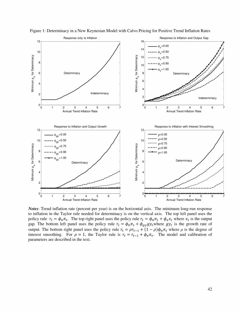
42
Figure 1: Determinacy in a New Keynesian Model with Calvo Pricing for Positive Trend Inflation Rates
Notes: Trend inflation rate (percent per year) is on the horizontal axis. The minimum long-run response
to inflation in the Taylor rule needed for determinacy is on the vertical axis. The top left panel uses the
policy rule �� = 78�. The top right panel uses the policy rule �� = 78� + 7:�� where �� is the output
gap. The bottom left panel uses the policy rule �� = 78� + 7CD���where ��� is the growth rate of
output. The bottom right panel uses the policy rule �� = L���� + �1 − L�78� where ρ is the degree of
interest smoothing. For L = 1, the Taylor rule is �� = ���� + 78� . The model and calibration of
parameters are described in the text.
0 1 2 3 4 5 6 70
2
4
6
8
10
12Response only to Inflation
Annual Trend Inflation Rate
Min
imum
φπ f
or
Dete
rmin
acy
0 1 2 3 4 5 6 70
2
4
6
8
10
12Response to Inflation with Interest Smoothing
Annual Trend Inflation Rate
Min
imum
φπ f
or
Dete
rmin
acy
0 1 2 3 4 5 6 70
2
4
6
8
10
12Response to Inflation and Output Growth
Annual Trend Inflation Rate
Min
imum
φπ f
or
Dete
rmin
acy
0 1 2 3 4 5 6 70
2
4
6
8
10
12
14
16Response to Inflation and Output Gap
Annual Trend Inflation Rate
Min
imum
φπ f
or
Dete
rmin
acy
ρ=0.00
ρ=0.50
ρ=0.75
ρ=0.90
ρ=1.00
φgy=0.00
φgy=0.50
φgy=0.75
φgy=0.90
φgy=1.00
φx=0.00
φx=0.50
φx=0.75
φx=0.90
φx=1.00
DeterminacyDeterminacy
DeterminacyDeterminacy
Indeterminacy
Indeterminacy

43
Figure 2: The Effects of Trend Inflation within the Determinacy Region
Notes: The figure plots the central bank’s minimal response to inflation required to maintain a given level
of utility for different levels of trend inflation relative to the minimal response to inflation necessary to
maintain this level of utility for zero trend inflation. The policy rule is �� = 78�. The utility level is
computed using the second order approximation to consumer utility with habit formation in consumption.
Habit is governed by the parameter h. See text for further details.
0 1 2 3 4 5 61
1.2
1.4
1.6
1.8
2
2.2
2.4
2.6
2.8R
ela
tive r
esponse t
o inflation
Trend inflation, percent per year
h=0.1
h=0.5
h=0.9

44
Figure 3: Time-Varying Parameter Estimates of the Taylor Rule
Notes: The figure presents time-varying parameter estimates of the Taylor rule, equation (7) in the text, under the assumption that parameters follow random walks.
Smoothed estimates from the Kalman filter are reported. We allow for two breaks in volatility of the shocks to parameters: 1979 and 1982. Dashed lines indicate
one standard deviation confidence intervals. Trend inflation is extracted from the time-varying constant as explained in section III.D. Point estimates and
confidence intervals are smoothed (moving average over five FOMC meetings) for expositional purposes. The sum of autoregressive coefficients in the Taylor rule
is adjusted to quarterly frequency because pre-1979 and post-1982 periods have different frequency of FOMC meetings.
1969 1972 1975 1978 1981 1984 1987 1990 1993 1996 1999 20021
1.5
2
2.5
3
3.5
φπ,t
1969 1972 1975 1978 1981 1984 1987 1990 1993 1996 1999 20020
0.5
1
1.5
2
2.5
φgy,t
1969 1972 1975 1978 1981 1984 1987 1990 1993 1996 1999 20020
0.2
0.4
0.6
0.8
1
φx,t
1969 1972 1975 1978 1981 1984 1987 1990 1993 1996 1999 2002
0.4
0.6
0.8
1
ρ1,t + ρ2,t
1969 1972 1975 1978 1981 1984 1987 1990 1993 1996 1999 2002-2
-1
0
1
2
ct
1969 1972 1975 1978 1981 1984 1987 1990 1993 1996 1999 2002
0
2
4
6
8
10
Trend inflation
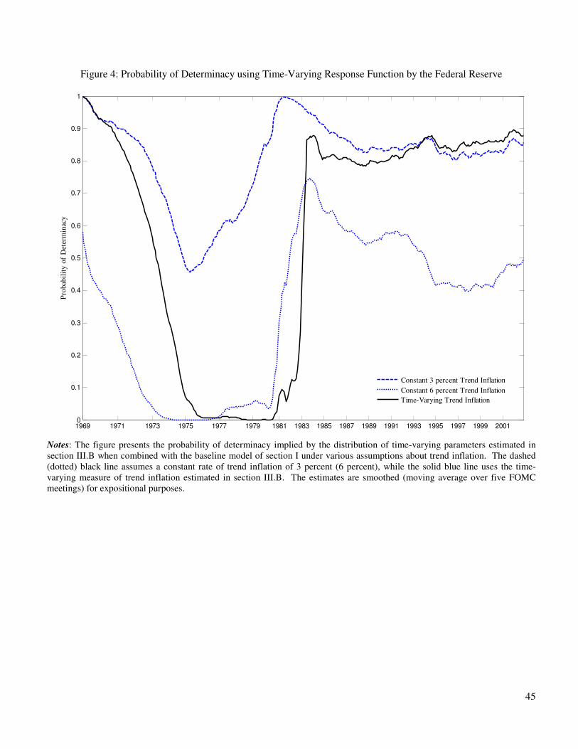
45
Figure 4: Probability of Determinacy using Time-Varying Response Function by the Federal Reserve
Notes: The figure presents the probability of determinacy implied by the distribution of time-varying parameters estimated in
section III.B when combined with the baseline model of section I under various assumptions about trend inflation. The dashed
(dotted) black line assumes a constant rate of trend inflation of 3 percent (6 percent), while the solid blue line uses the time-
varying measure of trend inflation estimated in section III.B. The estimates are smoothed (moving average over five FOMC
meetings) for expositional purposes.
1969 1971 1973 1975 1977 1979 1981 1983 1985 1987 1989 1991 1993 1995 1997 1999 20010
0.1
0.2
0.3
0.4
0.5
0.6
0.7
0.8
0.9
1
Pro
bab
ilit
y o
f D
eter
min
acy
Constant 3 percent Trend Inflation
Constant 6 percent Trend Inflation
Time-Varying Trend Inflation
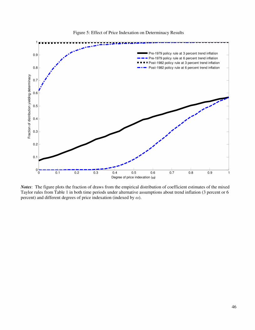
46
Figure 5: Effect of Price Indexation on Determinacy Results
Notes: The figure plots the fraction of draws from the empirical distribution of coefficient estimates of the mixed
Taylor rules from Table 1 in both time periods under alternative assumptions about trend inflation (3 percent or 6
percent) and different degrees of price indexation (indexed by ω).
0 0.1 0.2 0.3 0.4 0.5 0.6 0.7 0.8 0.9 10
0.1
0.2
0.3
0.4
0.5
0.6
0.7
0.8
0.9
1
Degree of price indexation (ω)
Fra
ction o
f dis
trib
ution y
ield
ing d
ete
rmin
acy
Pre-1979 policy rule at 3 percent trend inflation
Pre-1979 policy rule at 6 percent trend inflation
Post-1982 policy rule at 3 percent trend inflation
Post-1982 policy rule at 6 percent trend inflation
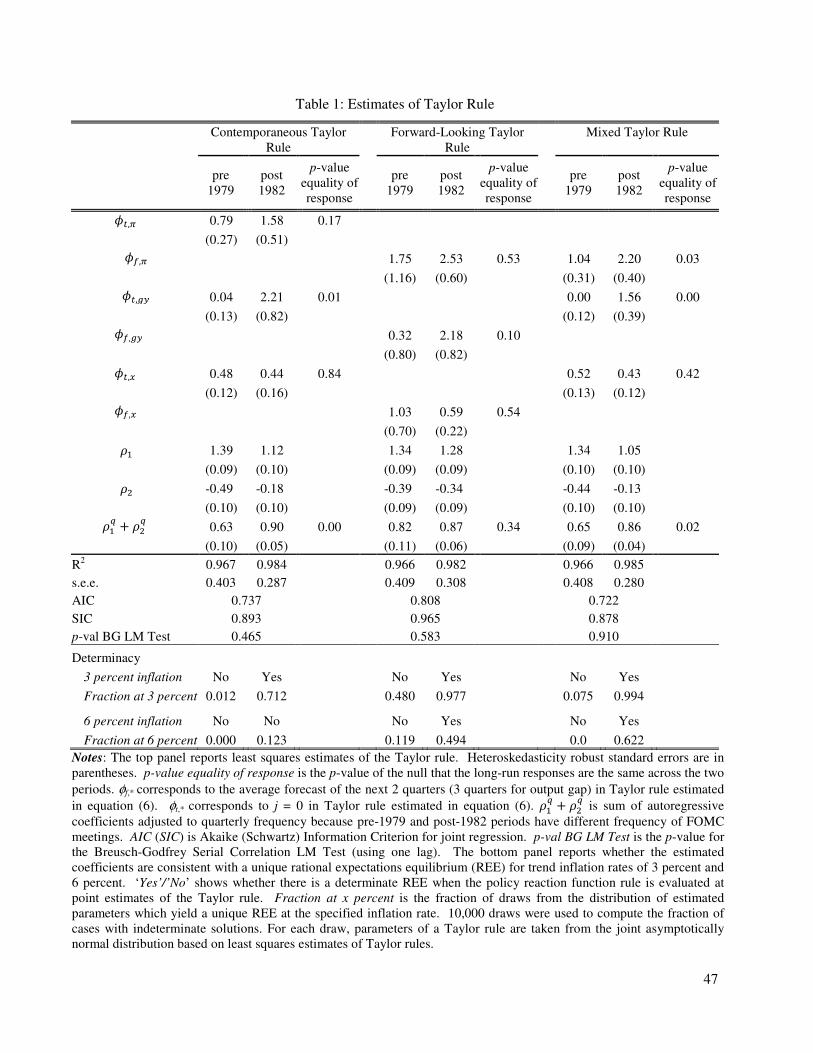
47
Table 1: Estimates of Taylor Rule
Contemporaneous Taylor
Rule
Forward-Looking Taylor
Rule
Mixed Taylor Rule
pre
1979
post
1982
p-value
equality of
response
pre
1979
post
1982
p-value
equality of
response
pre
1979
post
1982
p-value
equality of
response
7�,8 0.79 1.58 0.17
(0.27) (0.51)
7z,8 1.75 2.53 0.53 1.04 2.20
0.03
(1.16) (0.60) (0.31) (0.40)
7�,CD 0.04 2.21 0.01 0.00 1.56
0.00
(0.13) (0.82) (0.12) (0.39)
7z,CD 0.32 2.18 0.10
(0.80) (0.82)
7�,: 0.48 0.44 0.84 0.52 0.43
0.42
(0.12) (0.16) (0.13) (0.12)
7z,: 1.03 0.59 0.54
(0.70) (0.22)
L� 1.39 1.12 1.34 1.28 1.34 1.05
(0.09) (0.10) (0.09) (0.09) (0.10) (0.10)
L� -0.49 -0.18 -0.39 -0.34 -0.44 -0.13
(0.10) (0.10) (0.09) (0.09) (0.10) (0.10)
L�{ + L�{ 0.63 0.90 0.00 0.82 0.87 0.34 0.65 0.86
0.02
(0.10) (0.05) (0.11) (0.06) (0.09) (0.04)
R2 0.967 0.984 0.966 0.982 0.966 0.985
s.e.e. 0.403 0.287 0.409 0.308 0.408 0.280
AIC 0.737 0.808 0.722
SIC 0.893 0.965 0.878
p-val BG LM Test 0.465 0.583 0.910
Determinacy
3 percent inflation No Yes No Yes No Yes
Fraction at 3 percent 0.012 0.712 0.480 0.977 0.075 0.994
6 percent inflation No No No Yes No Yes
Fraction at 6 percent 0.000 0.123 0.119 0.494 0.0 0.622
Notes: The top panel reports least squares estimates of the Taylor rule. Heteroskedasticity robust standard errors are in
parentheses. p-value equality of response is the p-value of the null that the long-run responses are the same across the two
periods. φf,* corresponds to the average forecast of the next 2 quarters (3 quarters for output gap) in Taylor rule estimated
in equation (6). φt,* corresponds to j = 0 in Taylor rule estimated in equation (6). L�{ + L�{ is sum of autoregressive
coefficients adjusted to quarterly frequency because pre-1979 and post-1982 periods have different frequency of FOMC
meetings. AIC (SIC) is Akaike (Schwartz) Information Criterion for joint regression. p-val BG LM Test is the p-value for
the Breusch-Godfrey Serial Correlation LM Test (using one lag). The bottom panel reports whether the estimated
coefficients are consistent with a unique rational expectations equilibrium (REE) for trend inflation rates of 3 percent and
6 percent. ‘Yes’/’No’ shows whether there is a determinate REE when the policy reaction function rule is evaluated at
point estimates of the Taylor rule. Fraction at x percent is the fraction of draws from the distribution of estimated
parameters which yield a unique REE at the specified inflation rate. 10,000 draws were used to compute the fraction of
cases with indeterminate solutions. For each draw, parameters of a Taylor rule are taken from the joint asymptotically
normal distribution based on least squares estimates of Taylor rules.
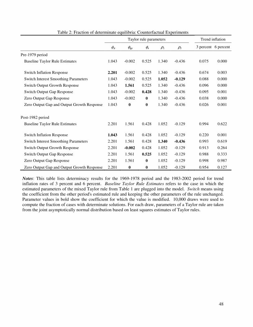
48
Table 2: Fraction of determinate equilibria: Counterfactual Experiments
Taylor rule parameters
Trend inflation
φπ φgy φx ρ1 ρ2
3 percent 6 percent
Pre-1979 period
Baseline Taylor Rule Estimates 1.043 -0.002 0.525 1.340 -0.436 0.075 0.000
Switch Inflation Response 2.201 -0.002 0.525 1.340 -0.436 0.674 0.003
Switch Interest Smoothing Parameters 1.043 -0.002 0.525 1.052 -0.129 0.088 0.000
Switch Output Growth Response 1.043 1.561 0.525 1.340 -0.436 0.096 0.000
Switch Output Gap Response 1.043 -0.002 0.428 1.340 -0.436 0.095 0.001
Zero Output Gap Response 1.043 -0.002 0 1.340 -0.436 0.038 0.000
Zero Output Gap and Output Growth Response 1.043 0 0 1.340 -0.436 0.026 0.001
Post-1982 period
Baseline Taylor Rule Estimates 2.201 1.561 0.428 1.052 -0.129 0.994 0.622
Switch Inflation Response 1.043 1.561 0.428 1.052 -0.129 0.220 0.001
Switch Interest Smoothing Parameters 2.201 1.561 0.428 1.340 -0.436 0.993 0.619
Switch Output Growth Response 2.201 -0.002 0.428 1.052 -0.129 0.913 0.264
Switch Output Gap Response 2.201 1.561 0.525 1.052 -0.129 0.988 0.333
Zero Output Gap Response 2.201 1.561 0 1.052 -0.129 0.998 0.987
Zero Output Gap and Output Growth Response 2.201 0 0 1.052 -0.129 0.954 0.127
Notes: This table lists determinacy results for the 1969-1978 period and the 1983-2002 period for trend
inflation rates of 3 percent and 6 percent. Baseline Taylor Rule Estimates refers to the case in which the
estimated parameters of the mixed Taylor rule from Table 1 are plugged into the model. Switch means using
the coefficient from the other period's estimated rule and keeping the other parameters of the rule unchanged.
Parameter values in bold show the coefficient for which the value is modified. 10,000 draws were used to
compute the fraction of cases with determinate solutions. For each draw, parameters of a Taylor rule are taken
from the joint asymptotically normal distribution based on least squares estimates of Taylor rules.

49
Table 3. Robustness of Determinacy Results
Pre-1979 period Post-1982 period
Determinacy
at point
estimates
Fraction of
determinate
equilibria given
sampling
uncertainty
Determinacy
at point
estimates
Fraction of
determinate
equilibria given
sampling
uncertainty
Bils and Klenow (2004) Case (change prices every 5 months) 3 percent inflation No 0.169 Yes 0.995
6 percent inflation No 0.000 Yes 0.933
Nakamura and Steinsson (2008) Case (change prices every 10 months) 3 percent inflation No 0.000 No 0.420
6 percent inflation No 0.000 No 0.001
Taylor Staggered Price Setting (duration of 9 months) 3 percent inflation No 0.309 Yes 0.997
6 percent inflation No 0.071 Yes 0.995
Lower elasticity of substitution θ = 6
3 percent inflation No 0.373 Yes 0.999
6 percent inflation No 0.101 Yes 0.996
Lower elasticity of substitution θ = 6 and Nakamura and Steinsson (2008) Case 3 percent inflation No 0.080 Yes 0.994
6 percent inflation No 0.000 Yes 0.602
Notes: The table presents robustness results of determinacy from Table 1. ‘Yes’/’No’ shows whether there is a
determinate rational expectations equilibrium when the policy reaction function is evaluated at point estimates of the
Taylor rule. 10,000 draws were used to compute the fraction of cases with determinate solutions. For each draw,
parameters of a Taylor rule are taken from the joint asymptotically normal distribution based on least squares estimates
of Taylor rules.


