
Monopolistic Competition and Trade

Empirical phenomenon of intra-industry trade
● Neoclassical trade theory predicts inter-industry trade based on differences in technology and/or factor endowments
● Empirical analysis of European Economic Community (EEC) found evidence for intra-industry trade (IIT)
● Early work focused on measurement, Balassa (1965), Grubel and Lloyd (1975)
● Overlap in trade flows, i.e., Grubel and Lloyd index:
(1)
j j
j
j j
X M
GL =X M
-
1-( + )
jGL0≤ ≤1

Monopolistic competition and trade
● Observed IIT a key challenge to neoclassical orthodoxy
(Leamer, 1992)
● Monopolistic competition has become standard model
for rationalizing IIT
● Different models of monopolistic competition developed
based on preference structure:
■ Krugman (1979;1980) uses Dixit and Stiglitz’s (1977)
“love of variety” approach to preferences
■ Helpman (1981) uses Lancaster’s (1977)
“characteristics” approach to preferences

Monopolistic competition and trade
● Following Krugman (1980), economy under autarky
consists of single industry producing variety of goods
● All varieties enter utility symmetrically, consumers
having utility function:
(2)
where ci is consumption of ith good, and elasticity of
substitution between two goods is a constant
● If w is income, consumers maximize utility subject to
budget constraint, :
(3)
θ
iU = c θ i n, 0 < <1, =1,....,
σ = θ1/ (1- )
i iw = p x
θ
i iθc = λp i n-1 , =1,...,

Monopolistic competition and trade
● Labor is only factor, all goods being produced with
same cost function:
(4)
li is labor used in producing ith good, xi is output of ith
good, α are fixed costs, β are constant marginal costs
● Output of any good equals consumption, so assuming
consumers are workers, output of any good is
consumption of aggregate labor force:
(5)
and assuming full employment,
i il = α + βx α β > i n, , 0, =1,...,
i ix = Lc i n, =1,...,
iL = α + βx( )

Monopolistic competition and trade
● Assuming monopolistic competition, where equilibrium
is symmetric with prices and quantities identical across
goods, inverse demand for each firm is:
(6)
● Elasticity of demand defined as, , where
profit maximization implies,
● Profit-maximizing price will be:
(8)
● Firm’s profits being:
(9)
θp = θλ (x L-1 -1/ )
ε = θ σ1/ (1- ) =
mc = mr = p ε(1-1/ )
p = θ βw-1
π = px α + βx w- ( )

Monopolistic competition and trade
● Using (8), (9) can be solved for x:
(10)
● Given full employment, and (16), equilibrium number of
goods under autarky is:
(11)
i.e., number of goods is a function of size of labor force
L, level of fixed costs α and value of θ
● Trading with an identical economy, number of goods
will be 2n, as L has doubled
● Each good only produced in one country, sold in both
x = α p w β αθ β θ/ ( / - ) = / (1- )
n = L α + βx L θ α/ ( ) = (1- ) /

Monopolistic competition and trade
● Gains from trade are greater diversity as consumers
spread incomes over twice as many goods – firms have
same level of output in equilibrium as under autarky
● Also in trading equilibrium, prices of any good in either
country are the same, and real wages are the same, i.e.,
factor-price equalization
● Volume of trade is determinate, each country exporting
half the output of its goods, but direction of trade
indeterminate, i.e., arbitrary which country produces
which goods
● General equilibrium version of model developed by
Helpman and Krugman (1985)

Monopolistic competition and trade
● Assume two countries j and k, two factors, K and L, two
industries: competitive Z producing homogeneous
good under constant returns, and monopolistically
competitive X producing nx varieties under increasing
returns
● Figure 1 shows combined factor endowments of j and k,
where with full employment, is fully utilized, OQ of
resources used in X, and OQ* used in Z, and vector OO*
can be interpreted as world GDP, Yw
● Define OQO*Q* as factor-price equalization set (FPE), if
endowment is E, country j devotes resources to X
and OZ to Z
V
j
xOn

Monopolistic competition and trade
● BB through E, with slope of w/r gives income levels of
Yj=OC and Yk=CO* on diagonal OO*, all income going to
factors and spent on consumption
● Cx and Cz are consumption of X and Z by country j, and
there is simultaneous inter and intra-industry trade:
- j imports Z from k, and is net-exporter of X
- k exports Z to j, and is net-importer of X
- Net trade flows in X occur because
● Capital-abundant country j is net-exporter of capital-
intensive good, and labor-abundant country k exports
labor-intensive good (H-O model)
( - )j
x xn C
k
x xC n( - )
>j k
x xn n

O
B
B
Q
C
Q*
K
L
XC
jxn
Figure 1: Trade Equilibrium
ZC
E
Z
O* =V
w/r
L*
K*

Monopolistic competition and trade
● Key empirical prediction: share of IIT larger between
countries that are similar in terms of factor endowments
and relative size
● Helpman’s (1987) results support prediction using 4-
digit SITC data for 14 OECD countries over period 1970-
81:
(12)
● Hummels and Levinsohn (1995) re-ran (12) for 1962-83
with GDP/worker – replicated Helpman and Krugman
j kjk j kj k
Y YGL =α+βlog +β min logY logYN N1 2
- ( , )
j jkk+β max logY logY +μ3
,( , ) β β β31 2<0<0, >0,

Monopolistic competition and trade
● Key empirical prediction: volume of trade as share of
GDP increases as countries become more similar in
size – assuming structure of monopolistic competition
● Helpman’s (1987) results support prediction with data
for 14 OECD countries over period 1956-81:
(13)
where for country group A, VA is volume of trade, YA is
aggregate GDP, eA is share of world GDP, and is
share of j’s GDP in A’s GDP
● Right-hand side of (13) is measure of size dispersion –
increases as countries become more similar in size
A j
A AAj A
V =e eY
21- ( )
j
Ae

Empirical evaluation of monopolistic
competition story
● (13) is a form of gravity model – but it seems to fit trade
in both differentiated and homogeneous goods
● Empirical issue becomes one of determining which
theoretical model works best in a given data sample
(Evenett and Keller, 2002)
● Gravity equation predicts volume of trade between two
countries will be proportional to their GDPs and
inversely related to any trade barriers between them –
typical specification:
(14) ββ β βjk j k jk jk jkV = β Y Y D (A u31 2 4
0( ) ( ) ( ) )
Empirical evaluation of monopolistic
competition story
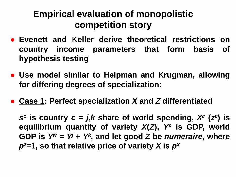
● Evenett and Keller derive theoretical restrictions on
country income parameters that form basis of
hypothesis testing
● Use model similar to Helpman and Krugman, allowing
for differing degrees of specialization:
● Case 1: Perfect specialization X and Z differentiated
sc is country c = j,k share of world spending, Xc (zc) is
equilibrium quantity of variety X(Z), Yc is GDP, world
GDP is Yw = Yj + Yk, and let good Z be numeraire, where
pz=1, so that relative price of variety X is px

Empirical evaluation of monopolistic
competition story
● Assuming balanced trade, where sc = Yc/Yw, both
countries demand all varieties according to their share
of world GDP, imports being given as:
(15)
(16)
where terms in brackets are GDP of k and j respectively,
therefore:
(17)
i.e., gravity equation, imports being proportional to GDP
jk j k k k k
x x zM = s p n x + n z[ ]
kj k j j j j
x x zM = s p n x + n z[ ]
j kjk j k k j kj
w
Y YM = s Y = = s Y = M
Y

Empirical evaluation of monopolistic
competition story
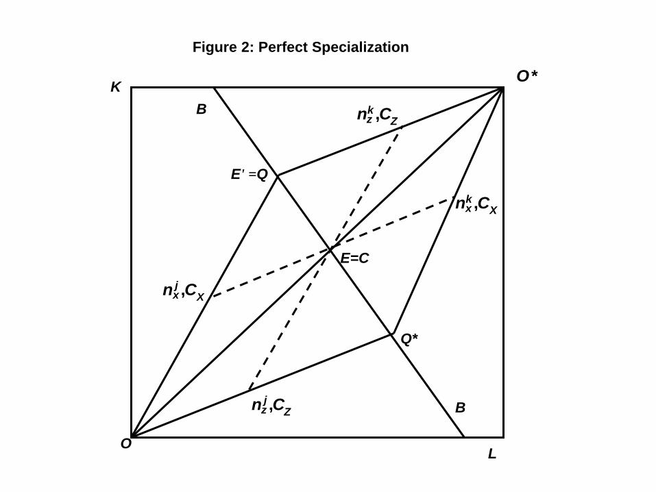
● Case 2: Perfect specialization, X and Z homogeneous
Assume X is capital-intensive and Y labor-intensive, j
being relatively well-endowed in capital, and k in labor
With perfect specialization, Xc production of X, Zc of Z,
Xj = Xw, and Zk = Zw, and value of production is GDP,
pxXj=Yj and Zk = Yk, therefore:
(18)
Identical to (17), and again imports are proportional to
GDP - known as multi-cone H-O model
Both equilibria can be described in figure 2
j kjk j k j k
w
Y YM = s Z = s Y =
Y,
j kkj k j k j
x w
Y YM = s p X = s Y =
Y
O
B
B
E' =Q
E=C
Q*
K
L
kx X
n C,
Figure 2: Perfect Specialization
O*
jz Z
n C,
kz Z
n C,
jx X
n C,

Empirical evaluation of monopolistic
competition story
● Case 3: Imperfect specialization X differentiated and Z
homogeneous
Assume X is capital-intensive and Y labor-intensive, j
being relatively well-endowed in capital, and k in labor
For endowments inside FPE, volume of bilateral trade:
(19)
where first term on right-hand side is j’s exports, other
terms are its imports of other varieties of X and good Z,
i.e. Mjk
jk k j j k k k w
x xT = s p X + s p X + Z s Z( - )

Empirical evaluation of monopolistic
competition story
● Suppose , share of Z in j’s GDP, and
also share of X in j’s GDP
With balanced trade, Mkj = skpxXj, then
Gravity equation (17) can be rewritten as:
(19)
Compared to (17), implies bilateral imports lower than
case where both goods are differentiated, and volume
of trade higher, the lower is share of Z in GDP
j j
x j jγ = Z p X + Z/jγ(1- )
kj k j jM = s γ Y(1- )
j kjk j
w
Y YM = γ
Y(1- )

Empirical evaluation of monopolistic
competition story
● Case 4: Imperfect specialization, X and Z homogeneous
Volume of bilateral trade:
(20)
where first term on right-hand side is j’s exports, and
second term are its imports, and Mjk = Mkj
Given Xw = (Xj +Xk), Mjk can be rewritten as:
and with , this becomes:
jk j j w k k w
xT = p X s X + Z s Z( - ) ( - )
jk j j j j j j k kM γ Y s γ Y s γ Y= (1- ) - (1- ) - (1- )
= (1- )k js s
jk k j j j k kM s γ Y s γ Y= (1- ) - (1- )

Empirical evaluation of monopolistic
competition story
● The gravity equation becomes:
(21)
As capital-labor ratios of two countries converge, so
that , and in the limit, no trade when
If , (18) is special case of (21)
● (19) and (21) are illustrated in figure 3, i.e., either intra-
industry trade in X, inter-industry in X and Z, or inter-
industry trade in X and Z (uni-cone H-O model)
j kjk k j
w
Y YM γ γ
Y= ( - )
k jγ γ k jγ = γ
k jγ = γ0, and =1

O
B
B
Q
C
Q*
K
L
kxn X,
Figure 3: Imperfect Specialization
O*
ZC
ZC
XC
E
jxn X,
Z
Z
XC
Empirical evaluation of monopolistic
competition story
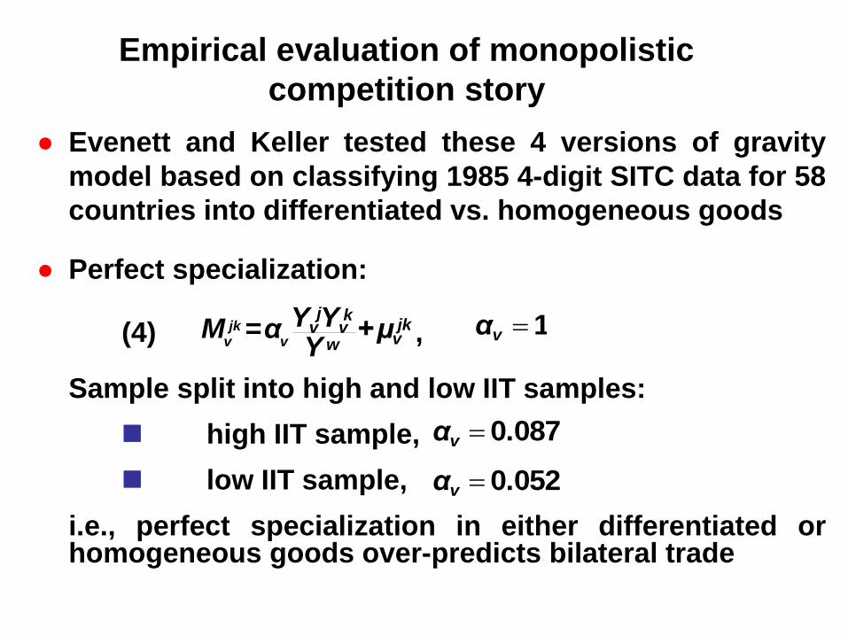
● Evenett and Keller tested these 4 versions of gravity
model based on classifying 1985 4-digit SITC data for 58
countries into differentiated vs. homogeneous goods
● Perfect specialization:
(4) ,
Sample split into high and low IIT samples:
high IIT sample,
low IIT sample,
i.e., perfect specialization in either differentiated or homogeneous goods over-predicts bilateral trade
jkv v
j kjkv v
vw
Y YM =α +μY
1vα
0.087vα
0.052vα

Empirical evaluation of monopolistic
competition story
● Imperfect specialization with differentiated and
homogeneous goods:
(5) ,
Estimated for cases where j(k) is capital-abundant,
median value of
● Imperfect specialization with homogeneous goods:
(6) ,
Estimated for cases where j(k) is capital-abundant,
median value of
j k
jk j jkv vv v vw
Y YM ψ μ
Y(1 ) (1- ) <1j
vψ
(1- ) = 0.086j
vψ
j k
v v
j kjk jkv v
v vw
Y YM ψ ψ μ
Y( ) ( - ) <1j k
v vψ ψ
( - ) = 0.04j k
v vψ ψ

Empirical evaluation of monopolistic
competition story
● Evenett and Keller conclude:
perfect specialization in increasing returns and multi-
cone model over-predicts bilateral trade
mixed support for increasing returns model with
imperfect specialization
uni-cone H-O model works well
● Overall, both factor endowments and scale economies
can explain different components of variations in
production and trade


