
Catalog No. L00310e
Movement of Underground Water in Contact with Natural Gas
Contract NO-31
Prepared for the Underground Storage Committee
Pipeline Research Committee
of Pipeline Research Council International, Inc.
Prepared by the following Research Agencies:
The University of Michigan
Authors: Donald L. Katz M. Rasin Tek
Keith H. Coats Marvin L. Katz
Stanley C. Jones Maurice C. Miller
Publication Date: February 1963

“This report is furnished to Pipeline Research Council International, Inc. (PRCI) under the terms of PRCI NO-31, between PRCI and The University of Michigan. The contents of this report are published as received from The University of Michigan. The opinions, findings, and conclusions expressed in the report are those of the authors and not necessarily those of PRCI, its member companies, or their representatives. Publication and dissemination of this report by PRCI should not be considered an endorsement by PRCI or The University of Michigan, or the accuracy or validity of any opinions, findings, or conclusions expressed herein. In publishing this report, PRCI makes no warranty or representation, expressed or implied, with respect to the accuracy, completeness, usefulness, or fitness for purpose of the information contained herein, or that the use of any information, method, process, or apparatus disclosed in this report may not infringe on privately owned rights. PRCI assumes no liability with respect to the use of, or for damages resulting from the use of, any information, method, process, or apparatus disclosed in this report. The text of this publication, or any part thereof, may not be reproduced or transmitted in any form by any means, electronic or mechanical, including photocopying, recording, storage in an information retrieval system, or otherwise, without the prior, written approval of PRCI.”
Pipeline Research Council International Catalog No. L00310e
Copyright, 1963 All Rights Reserved by Pipeline Research Council International, Inc.
PRCI Reports are Published by Technical Toolboxes, Inc.
3801 Kirby Drive, Suite 340 Houston, Texas 77098 Tel: 713-630-0505 Fax: 713-630-0560 Email: [email protected]

ACKNOWLEDGMENT
During the three-year tenure of Project NO-31 “Engineering Studies on Movement of
Water in Contact with Natural Gas” many individuals from the Pipeline Research Council International,
Inc., Industry and The University of Michigan actively participated in several phases of this investi-
gation.
The assistance given by the Supervising Committee, John A. Vary, Chairman, and
Messrs. O. C. Davis, B. B. Gibbs, E. V. Martinson, C. E. Stout and S. J. Cunningham is grate-
fully acknowledged. The contacts with the Pipeline Research Council International, Inc. were maintained
by Mr. S. J. Cunningham and later by Messrs. Roger Duke and Thomas E. Walsh, his alternates. Messrs.
Charles A. Hutchinson, Jr. and Phillip H. Braun actively participated in the work of the Super-
vising Committee, representing the American Petroleum Institute.
Messrs. J. R. Elenbaas, R. M. Hubbard and Milton A. Surles participated in committee
meetings. Advice and suggestions were offered by V. J. Berry, Jr.
The initation of basic research on the movement of water in underground gas storage
fields by the Michigan Gas Association fellowship at The University of Michigan in 1956 is
acknowledged.
Impetus to the present research was given in September 1958 by the Underground
Storage Committee of the Pipeline Research Council International, Inc. when it recommended that the
proposal for the project be submitted to the Pipeline Research Committee.
The cooperation of several companies from the oil, gas producing and gas storage indus-
tries in providing the field data so essential to this project is acknowledged.
i

This Page Intentionally Left Blank
PIPELINE RESEARCH COUNCIL INTERNATIONAL, INC.
Project NO-31 at The University of Michigan is conducted under the auspices of the
Pipeline Research Committee:
N. B. LauBach, (CHAIRMAN), Senior Vice PresidentColorado Interstate Gas Company, P. O. BOX 1087, Colorado Springs, Colorado
G. P. Binder, (VICE CHAIRMAN), Chief EngineerThe East Ohio Gas Company, 1717 East Ninth Street, Cleveland 14, Ohio
T. S. Bacon, Vice President i/c Research & DevelopmentLone Star Gas Company, 301 South Harwood Street, Dallas 1, Texas
S. A. Bergman, Chief EngineerPanhandle Eastern Pipe Line Company, P. O. Box 1348, Kansas City 41, Missouri
O. W. Clark, Senior Vice PresidentSouthern Natural Gas Company, P. O. Box 2563, Birmingham 1, Alabama
B. J. Clarke, Vice President i/c Engineering and ResearchColumbia Gas System Service Corporation, 120 East Forty-first Street, New York 17,New York
M. V. Cousins, Vice PresidentUnited Gas Pipe Line Company, P. O. Box 1407, Shreveport 92, Louisiana
R. H. Crowe, Chief EngineerTranscontinental Gas Pipe Line Corporation, P. O. Box 296, Houston 1, Texas
J. F. Eichelmann, Vice President & Executive EngineerEl Paso Natural Gas Company, P. O. Box 1492, El Paso, Texas
J. L. Gere, Chief EngineerCities Service Gas Company, Box 1995, Oklahorna City 1, Oklahoma City 1, Oklahoma
B. D. Goodrich, Senior Vice PresidentTexas Eastern Transmission Corporation, P. O. Box 2521, Houston 1, Texas
W. B. Haas, Vice PresidentNorthern Natural Gas Company, 2223 Dodge Street, Omaha 1, Nebraska
C. S. Kenworthy, General Superintendent of the Compressor Station DivisionNatural Gas Pipeline Company of America, 122 South Michigan Avenue, Chicago 3, Illinois
R. D. Morel, Pipeline SuperintendentAlgonquin Gas Transmission Company, 25 Faneuil Hall Square, Boston 9, Massachusetts
H. A. Proctor, Vice President, Engineering and TransmissionWouthern California Gas Company, Box 3249, Terminal Annex, Los Angeles 54, California
H. L. Stowers, Vice President i/c EngineeringTexas Gas Transmission Corporation, 3800 Frederica Street, Owensboro, Kentucky
i i

J. L. Thompson, Assistant to the PresidentMichigan Wisconsin Pipe Line Company, 500 Griswold Street, Detroit 26, Michigan
T. L. Robey, Director of ResearchPipeline Research Council International, Inc., 420 Lexington Avenue, New York 17, New York
S. J. Cunningham, Senior Research EngineerPipeline Research Council International, Inc., 420 Lexington Avenue, New York 17, New York
T. E. Walsh, (SECRETARY), Research EngineerPipeline Research Council International, Inc., 420 Lexington Avenue, New York 17, New York
The Supervising Committee for the project is:
J. A. Vary, (CHAIRMAN), Manager of Reservoir Engineering DepartmentMichigan Consolidated Gas Company, Grand Rapids, Michigan
O. C. Davis, General Superintendent, StorageNatural Gas Storage Company of Illinois, Chicago, Illinois
B. B. Gibbs, Assistant Superintendent, Geological DepartmentUnion Producing Company, Shreveport, Louisiana
E. V. Martinson, Director, Underground Storage DivisionNorthern Natural Gas Company, Omaha, Nebraska
C. E. Stout, Vice PresidentColumbia Gas System Service Corporation, New York, New York
T. E. Walsh, (SECRETARY), Research EngineerAmerican Gas Association, New York, New York
111

TABLE OF CONTENTS
AcknowledgmentForewordChapter 1. Aquifers in Gas Storage
Need for Study of Water Movement in Gas Storage OperationsNature of AquifersSignificance of StudySystem Calculations
Chapter 2. Flow Equations for Geometric ModelsDarcy’s Law - Steady StateUnsteady State FlowContinuity EquationDiffusivity EquationRadial Flow ModelLinear Flow ModelThick Sand ModelHemispherical Flow ModelElliptical Flow ModelComparisons of Dimensionless Functions
Chapter 3. Derivations of Flow Equations for ModelsRadial ModelLinear ModelThick Sand ModelHemispherical ModelElliptical Model
Chapter 4. Data Required for Field CalculationsFluid PropertiesReservoir PropertiesCalculation of Reservoir Pressure from Well. Head PressureInitial Gas Pore Volume
Chapter 5. Relating the Water Movement to the Gas Bubble PressureSuperposition PrincipleApplication of Superposition to Flow EquationsPrediction of Gas Reservoir PerformanceOptimizing Effective Values of Kr and KpOptimizing Initial Gas Pore Volume 1
Chapter 6. Generalized Method for PerformanceCalculation from Field DataThe Logic of the Resistance FunctionDevelopment of the ConceptCalculation of Resistance Function from Field DataSteps for Calculating the Field PerformanceSelf Correcting Features of the Computational ProcedureExtrapolation of the Resistance Function Curve
Chapter 7. Development of Aquifer Storage FieldsInsitu Permeability and CompressibilityEvaluation of Caprock from Pump TestsCalculation to Evaluate an Aquifer ProjectInitial Gas InjectionWater Movement CalculationsPressure Gradients in AquifersLocation of Gas-Water Contact (Bubble Edge)
pagei
v i i112
121 5171719192 223293 54 04 345494957606569737376818387889 19 59799
101101102103105109110113113120127129130132133
i v
Chapter 8. Special Topics in Gas StoragePound-Days as a GuideMoving Boundary Problem in Aquifer StorageMoving Boundary Approximation Based on Hemispherical ModelInterference Between Gas FieldsStratified FlowTwo-Phase FlowWater Drive Calculations with Analog Computers
Chapter 9. Demonstration of All Methods on Field AGeology and Field DataMachine CalculationsRadial Flow ModelLinear Flow ModelThick Sand ModelHemispherical ModelGeneralized Performance Method Using Resistance Function
Chapter 10. Case Studies - Production and Storage in Producing FieldsField B. Geology and Field Data
Calculations and ResultsField C. Geology and Field Data
Calculations and ResultsField D. Geology and Field Data
Calculations and ResultsField E. Geology and Field Data
Calculations and ResultsChapter 11. Case Studies - Aquifer Storage Fields
Field F. Geology and Field DataCalculations and Results
Field G. Geology and Field DataCalculations and Results
Field H. Geology and Field DataCalculations and Results
AppendixA. Table of Dimensionless Pressure, Pt, for Infinite Radial Aquifer,
Constant Terminal RateB. Table of Dimensionless Water Influx, Qt, for Infinite Radial Aquifer,
Constant Terminal PressureC. Table of Dimensionless Pressure, Pt, for Finite Radial Aquifer with
(Closed Exterior Boundary, Constant Terminal RateD. Table of Dimensionless Water Influx, Qt, for Finite Radial Aquifer with
(Closed Exterior Boundary, Constant Terminal PressureE. Table of Dimensionless Pressure, Pt, for Finite Radial Aquifer with
[Constant Pressure at Exterior Boundary, Constant Terminal RateF . Table of Dimensionless Pressure Drop Distribution, PD, (rD,tD), Finite
Radial Aquifer with Closed Exterior Boundary, Constant Terminal RateG. Table of Dimensionless Pressure Drop Distribution, PD(rD,tD), Finite
139139139142145147149152155155156158173176180184199199199205214218218225227233234237237243245245
2 5 1
2 5 2
2 5 5
2 5 6
2 6 0
263
Radial Aquifer with Closed Exterior Boundary Constant Terminal Pressure 2 6 5H. Table of Dimensionless Pressure Distribution, PD(xD,tD), Linear Flow
Aquifer with Closed Exterior Boundary, Constant Terminal Pressure 2 6 9I. Table of Dimensionless Pressure, Pt, for Infinite Thick Sand Aquifer,
Constant Terminal Rate 2 7 0J. Two Phase Flow During Growth of an Aquifer Storage Reservoir 272K. Computer Program for Radial Flow Model 276L . Computer Program for Linear Flow Model 289M. Computer Program for Resistance Function Method Including Moving
Boundary Modification 295
V

Nomenclature 312References 316Index 321
v i

This Page Intentionally Left Blank

FOREWORD
Prediction of water drive received its initial attention by the studies of Schilthuis and
Hurst in 1935 on the Woodbine aquifer adjacent to the East Texas Field. The next milestone in
computing aquifer behavior was the paper by Van Everdingen and Hurst in 1949. Engineering
studies of water drive occurring in gas storage reservoirs pointed out the need for more definite
procedures of calculation because of the cyclic nature of the storage operation. Research work
supported by the Michigan Gas Association was directed at understanding the effect of the cyclic
process on water movement. Due to the interest in aquifer storage fields and a recognition that
gas fields adjacent to aquifers experience water movement, the Underground Storage Committee
of the American Gas Association recommended sponsorship of the Research Project NO-31 under
the Pipeline Research Committee. Approval of the project was received in May 1959.
The first year of the project was devoted to developing equations and procedures to
ascertain, analyze and interpret the nature and the extent of water drive for various geometric
models. Solutions to the equations and procedures for calculation were developed during the
first year. Digital computing techniques were developed to permit the handling of the large
number of calculations required by the nature of the pressure cycles.
During the second year, field data were collected and analyzed for several storage and
production operations. The field data were employed to compare predicted performance with
observed behavior. These calculations required refinements and extensions of the equations
developed during the first year.
The organization of the entire material pertaining to the mathematical treatment of
water drive gas reservoirs, applications to field data, discussion of results and general con-
clusions were undertaken during the third and concluding year of the project.
The projected was conducted in the Department of Chemical and Metallurgical Engi-
neering at The University of Michigan under the direction of Dr. Donald L. Katz, Professor
of Chemical Engineering and Dr. M. Rasin Tek, Associate Professor of Chemical Engineering.
Dr. Keith H. Coats, Assistant Professor of Chemical Engineering at The University
of Michigan 1959-61 and currently at Jersey Production Research Company was an active par-
ticipant in the project while at the University.
Dr. Marvin L. Katz, currently with Sinclair Research, Inc., was a Fellow on the
project from July 1959 through November 1960. Messrs. Stanley C. Jones and Maurice C.
Miller were Fellows on the project from the summer of 1960 to its conclusion.
This Monograph is prepared for three groups: (1) the reservoir or field engineers for
gas storage and producing operations, (2) computing center personnel in gas companies who
are likely to become involved in water movement calculations, and (3) research engineers work-
ing on reservoir phenomena, who desire to find in one volume a summary of pertinent unsteady-
state flow equations and their solutions.
v i i

In the first chapter, the reader is introduced to the nature of aquifers. Water movement
calculations are shown to be necessary in most gas storage projects for predicting the pressure-
production or injection schedule for gas storage reservoirs as well as for verifying gas inventory.
The second chapter presents the working equations for predicting water movement for various
geometric models representing reservoir-aquifer systems, without going into detail of the mathe-
matical derivations. The models for the reservoir-aquifer systems considered in this monograph
have radial, linear, thick sand, hemispherical and elliptical flow geometries for the aquifer.
Detailed derivations of the unsteady-state flow equations and their solutions are presented for the
flow models in Chapter 3.
To use flow equations for practical field calculations it is necessary to be familiar with
such topics as the superposition principle, material balance on the gas reservoir, and bottom hole
versus well head pressures. These topics, along with a discussion of the data required in field
calculations, comprise Chapters 4 and 5.
A generalized performance calculation procedure is presented in Chapter 6. It is based
on direct field production-pressure data. Initially it employs a geometric idealization of the
reservoir, but the final calculation rests on the reservoir behavior. The method properly accounts
for the effect of irregular geometries and reservoir inhomogeneities. Since aquifer storage fields
are especially dependent upon water movement rates, Chapter 7 is devoted to their development.
Special topics such as a treatment of the moving boundary between the gas-water contact, inter-
ference between two or more gas reservoirs situated on the same aquifer, and the pound-day con-
cept in Chapter 8 conclude the background information for making field calculations.
In Chapter 9, a demonstration calculation is made for a single field, employing the formulas
for four models and the generalized performance calculation procedure. The concluding two chap-
ters cover the case studies for four production gas storage fields and three aquifer storage reser-
voirs. In each of the cases, the geology and early field data are used to predict the pressure-
injection or production behavior for comparison with actual behavior.
In the appendices, the reader will find the tables of functions which are used to simplify
the complex unsteady-state flow calculations. The computer programs for the demonstration cal-
culations of Chapter 9 are also presented in the appendices.
This Monograph covers the full range from the calculation procedures for practicing
engineers to the complex mathematical developments required in deriving the relationships used
and the computer programs for machine computations.
v i i i
CHAPTER 1.
AQUIFERS IN GAS STORAGE
Underground porous formations necessarily contain some fluid, either water, gas, oil
or combinations thereof. The pore space per unit of rock volume may be limited as in shale
comprising caprock - or it may be substantial as in productive zones. Pressure changes in
the reservoir gas phase create pressure gradients in the aquifer water phase, causing water
movement. Water entering the space originally occupied by gas influences the pressure of the
gas phase for a given amount of gas in place. Any study of gas reservoir pressures or of quan-
tities of gas in place must depend upon calculations of water movement. This chapter will point
out in more detail the need for understanding water movement, the nature of aquifers, and the
practical significance of the study.
Need for Study of Water Movement in Gas Storage Operations
The economic use of natural gas for space heating in northern regions requires the
storage of gas near the market in summer and the production of that gas during the winter. This
situation exists because the principal supply of gas is produced at considerable distance from a
major portion of the space heating market, and it is uneconomical to build long pipelines with
sufficient capacity to meet peak loads in winter. Since many distributing companies and pipe-
line systems depend upon underground storage for a substantial part of their send-out on a cold
winter day, considerable engineering and managerial effort goes into handling storage matters.
Because of this dependence on stored gas, it is natural that careful studies are now
made on gas storage fields. The operator is asked to predict the seasonal storage capacity and
field deliverability for winter operation. How much gas can a storage field deliver to market on
the last day of February with available compressors? How much gas can be stored in the field
next summer? How much gas do you lose in underground storage? These are the questions
which have provided the incentive to study underground storage operations.
The testing of gas well flow capacity and the plotting of pressure decline curves during
gas production were early techniques borrowed from gas production operations for use in
storage projects. The concept of water drive as a reservoir mechanism has been recognized
by the oil industry since the study made on the East Texas Oil Field (57). Any attempt to extend
the techniques established for oil or gas production to the operation of gas storage fields indicates
differences in applicability, mainly due to the special nature of storage operations.
The usual storage field is equipped to produce at rates so that its working storage gas
content can be produced in 30 to 120 days. Although gas producing fields may have excess flow
capacity, they seldom produce their reserve in less than five full years and more likely in 12 to
18 years. Well spacing in storage fields may be 20 to 40 acres, as compared to 160 or 640 acres
for production. Field pressure declines of 20 pounds per square inch per day are quite normal
1
Movement of Underground Water in Contact with Natural Gas
in storage; such rates might be considered excessive in production. Gas storage operations pre-
sent a much more variable pressure-time schedule than naturally producing reservoirs because
of the injection of gas in summer and withdrawal in winter. Approximate methods of predicting
water movement suitable for gas producing fields are not adequate for gas storage fields because
of the cyclic nature of the reservoir pressures.
The recent advent of aquifer storage is, perhaps, the most prominent example where
the information on the rate of water movement is required. In aquifer storage, the pore volume
necessary for the storage of gas is created by expulsion of water from its native formation by
pressurization above the initial discovery level. Initial. evaluation of a possible aquifer storage
project depends upon calculation of the rate at which gas can be injected to develop the gas bubble
(34)(35). The gas injection rate depends on the rate at which water may be moved within the
aquifer. Likewise, estimates of gas withdrawal during winter are dependent upon calculated rates
of water return and the resultant gas reservoir pressure.
In early gas storage practice, gas was injected into old gas fields to raise the pressure.
The level of pressure seldom reached the initial discovery value. Discovery pressure in many
instances corresponds to the hydrostatic pressure. This occurrence of petroleum and water in
underground strata at hydrostatic pressure is a verification of the concept that the pore space in
the earth’s crust is filled with water unless oil or gas are present. In recent years, gas reser-
voir pressures have been raised in storage fields above the initial or hydrostatic values, a prac-
tice described as “overpressuring”. The use of these higher pressures has increased the capacity
of storage fields significantly. Calculations of water movement become important in predicting
the effect of time at the overpressure condition on the growth of the gas bubble. Verification of
gas inventory in such fields requires a knowledge of water movement. Investigations of overpres-
sure effects on water movement in the research supported by the Michigan Gas Association devel-
oped quantitative methods for handling the cyclic pressure schedule (6)(33)(72).
This research was initiated to bring together the knowledge required to predict water
movement in gas storage operations. The goal was to develop calculation procedures which
could be utilized directly by engineers in charge of the operation of storage fields.
Nature of Aquifers
An aquifer is a water-filled blanket zone or layer of underground porous rock extending
for distances measured in miles. The study of the nature of aquifers is appropriate and essential
to understanding the movement of water in contact with natural gas. The aquifer rock is perme-
able enough so that water will move through the porous matrix at a significant rate when it is
subjected to a pressure gradient. Figure l-l from Hubberf (24) shows how water can flow under-
ground due to effects of gravity. The aquifer in Figure 1-1 takes in water at the outcrop updip
and the water moves toward an outcrop downdip. In this case, the water in the aquifer will be
fresh, at least near the intake, and may be potable throughout the extent of the blanket sand.
2

Aquifers in Gas Storage
Figure 1- 1 Regional Flow of Water through Sand from Higher to Lower Outcrop. (Hubbert)(24)(Courtesy Bull. AAPG)
A study of the Woodbine aquifer supplying water to the East Texas Oil Field shows that
pressure gradients may extend to distances of 100 miles (1). The Woodbine aquifer, Figure 1-2,
on the other hand, has no outlet for water and therefore contains the sea water prevalent at the
time when it was buried by the overburden. Thus the nature of water in blanket sands may vary
in character from essentially fresh water to nearly saturated brines, all depending upon the
geological history and communication with the surface through one or more outcrops.
The St. Peter, Galesville, and Mt. Simon formations are blanket sands extending over
much of northern Illinois and eastern Iowa. They are sources of potable water in the Chicago
area, which is not far from the outcrop occurring in Wisconsin. The Herscher storage project
has gas reservoirs in the Galesville and Mt. Simon sands (55). The Troy Grove project stores
gas in the Mt. Simon zone (69). The Redfield storage project in Iowa uses the St. Peter and Mt.
Simon strata. Water movement in these sands responds relatively rapidly to pressure changes,
and they are typical aquifers. On a given summer day, gas injection can displace 500,000 to
1,000,000 cubic feet of water per day from a reservoir, while during the low gas pressure season
after gas withdrawal, the influx of water can be two or three times this amount. These particular
aquifers are so large relative to the gas fields that they may be considered to be of infinite extent.
The Marshall standstone of Mississippian age covers much of Central Michigan, and is
considered to be an aquifer. While the permeability is not high enough to permit rapid water
movement, pressure gradients have been observed in this sand over a distance of miles. The
water in the Marshall formation contains a high concentration of salt, approaching saturation.
The stray sand gas fields in Central Michigan are used for gas storage as shown in Figure 1-3.
Brine movement takes place during storage cycles, but seldom changes the volume of the gas
reservoir by more than one to three per cent per year, even when the reservoir pressure is held
3


Figure 1-3 Water Level Changes in Michigan Stray Sand during Gas Storage.
for long periods either at low pressures or at some reasonable overpressure.
Generally this Monograph is concerned with water movement in an aquifer caused by
pressure fluctuations in an adjacent gas reservoir.
Water Movement in aquifers may be demonstrated by considering the behavior of a
group of wells completed in a shallow aquifer used as a source for potable water, Figure 1-4.
The diagram illustrates the water levels in adjacent wells when one of the wells is produced.
Water production lowers the pressure or head around the well bore and water flows towards
the supply well because it is at a lower pressure than the water in the sand some distance away.
Consider now a growing gas bubble in an aquifer gas storage project, Figure 1-5.
Gas is injected rapidly enough to hold the gas bubble at a pressure ∆ P above the initial
aquifer pressure. Water flows away from the gas bubble, causing it to expand.
5


Movement of Underground Water in Contact with Natural Gas
The pressure in the surrounding sand is raised as indicated at various successive times,
t1 , t2 , t3 etc. When water flows out from the gas bubble, where does it go? It simply com-
presses the water ahead of it. Since such movement is in a radial direction away from the
bubble, there is an increasing quantity of water associated with successive increments of
radial distance.
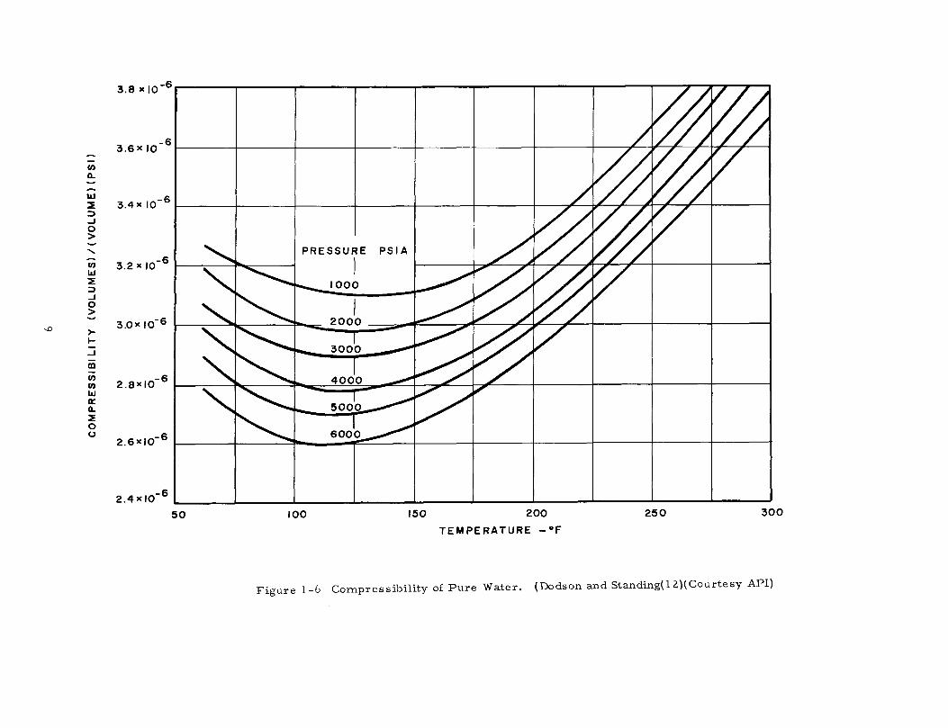
Water is among the least compressible of liquids. However, for every pound per
square inch rise on a million cubic feet of water, the million cubic feet will shrink by some
3.0 cubic feet. Thus the water compressibility is said to be 3.0 x 10⁻⁶(volumes)/(volume)(psi).
Figure 1-6 shows the compressibility of pure water (12). The compressibility of water varies
with mineral content and dissolved gases.
When porous sand containing water is subjected to pressure rise through water pres-
sure, the combined compression of the water and the rock is approximately twice that of pure
water (14)(17)(35). Therefore, if the above million cubic feet of water were contained in por-
ous sandstone of about 20 per cent porosity, a pressure rise of one pound per square inch wouldshrink the composite sand-water system by about seven cubic feet.
To help fix orders of magnitude, consider a gas field of 3,000 feet in radius sur-
rounded by a blanket water sand 100 feet thick with a porosity of 20 per cent. Raise the pres-
sure in the gas field by 300 pounds per square inch, causing the aquifer to have the pressure
distribution shown in Table 1-1 at some time t. Using the compressibility of water and that
of the porous formation, one can compute the combined compression of the water and rock as
shown in Table 1-1. Compression of water in the sand within a distance of 2.5 miles is
shown to cause 2.30 million cubic feet of water to be absorbed by the aquifer without any
movement beyond the 15,000 foot radius.
Table 1-1 Calculation of Water Compression by an Expanding Gas Reservoir.
* In this illustration, the arithmetic average is 2 per cent above the correct integrated aver-age pressure given by
**The procedure for estimating the pressure distribution is given on page 132.8

Movement of Underground Water in Contact with Natural Gas
In this example calculation, virtually no water movement occurs beyond a radius of
15,000 feet up to time t. This “radius of influence” will increase as time increases. If in
the time period of consideration in a field study (e. g. 20 years), the “radius of influence”
does not exceed the radius of the exterior aquifer boundary, then the aquifer is termed
“infinite." Thus we speak of an “infinite” aquifer when the exterior radius is so large that
water movement in the vicinity of this exterior boundary is negligible during the time period
under consideration.
Returning now to the gas bubble and surrounding aquifer of Figure 1-5, continued
pressurization of the gas bubble will cause water compression at further and further distances.
For the normal injection season, the distance may be some 3 to 6 miles before the pressure
is reduced in winter. However, in some cases the sand is not continuous in all directions
and may be limited in extent. Then the pressurization may take place to a greater degree
because of the reduced quantity of water affected.
Figure 1-7 shows a section of an aquifer limited by pinch out in one direction and
change into shale in the other. The volume of the gas reservoir might be five per cent of the
total sand volume. When gas pressure changes, water movement will take place, but to a
limited extent. Water movement caused by a pressure change of 1000 pounds per square
inch on a gas bubble occupying five per cent of the total pore space in a limited aquifer could
not change the volume of the bubble by more than t 13 per cent.
Figure 1-7 Section of a Limited Aquifer.
10

A limited aquifer may be described as a closed system. Typical examples of such
systems are found in the Ellenburger formation of West Texas and among the sand lenses of the
Illinois basis. Water movement into or out of a gas field situated on an aquifer may be restricted
due to the limited size of the water bearing sand or due to the low permeability of the blanket
sand. The Marshall sand in Michigan, Figure 1-3, permits only relatively small quantities of
water movement in a given gas injection or withdrawal season due to the low permeability of the
sand.
Water movement in an aquifer has been discussed without considering the nature of the
caprock confining the gas to the more permeable rock. Caprock is a low permeability and low
porosity layer, normally consisting of shale, limestone, or dolomite. It may have a porosity
from two to eight per cent and a permeability of 10-4 to less than 10-6 millidarcy. However,
this permeability is far too great for holding gas if water were not present in the pores of the
caprock.
The Threshold Pressure for gas to displace water from low permeability caprock core
is a measurement which may be made to evaluate caprocks. The permeability of the caprock
core may be 10-5 millidarcy and water will flow through such a core very slowly under a pres-
sure differential. However, if gas is brought to the face of the water saturated core, the flow
will stop if the pressure differential is below the threshold pressure for gas to displace water.
Threshold pressures of 100 to 500 pounds per square inch or more often are required for gas
to displace water from caprock cores with permeabilities of 10-4 to 10-6 millidarcy. Thus the
water in the caprock blocks the movement of gas and retains it in the reservoir. Figure 1-8
illustrates the water-gas contact at the top of the gas bearing zone and at the base of the water
bearing caprock.
When a gas reservoir or aquifer is discovered at hydrostatic pressure, then the pres-
sures in the caprock and in the porous aquifer formation would be in balance. However, when
gas is injected in an aquifer storage project, overpressure is required which in turn places a
pressure gradient across the caprock greater than the normal hydrostatic gradient. This over-
pressure must not exceed the threshold pressure for gas to displace water from the caprock,
for then gas would gradually permeate the caprock, dry it out, and start gas leakage. It should
be noted that all caprock leakage found to date is believed to be due to imperfections or discon-
tinuities in the caprock and not due to threshold displacement from relatively uniform caprock.
Low permeability rocks surrounding gas bubbles of normal gas fields are not limited
to the cap, but may also form the sides of the gas reservoir through transition from sand to
shale. Such gas reservoirs are described as sand lens or stratographic traps. In such cases,
not only is the top of the sand zone bounded by low permeability rock, but also the sides and even
the bottom. Horizontal water movement then would be similar to that described for vertical
movement at the interface between the porous sand and the caprock. Turn Figure 1-8 on its
side in visualizing the restraint which impervious rock places on gas and water movement.
11

Figure 1-8 The Water-gas Contact at the Base of the Caprock.
Many gas reservoirs in the Appalachian area are of the type just described.
Now that the nature of aquifers and their caprocks have been described, attention will
be turned to the significance of the study of water movement.
Significance of the Study
Experience with gas storage operations has shown that consideration of water move-
ment results in greatly increased accuracy in prediction of pressure and gas in place. It can
be maintained that three specific break-throughs of considerable significance were made when:
(1) Pressurization of gas reservoirs above discovery pressure was adopted for gas storage
fields, (2) Design procedures were developed for predicting the development rates of aquifer
storage projects, and (3) The effect and extent of water movement were ascertained on a quan-
titative basis for predicting the production-pressure behavior of storage reservoirs subject to
cyclic pressure changes. The use of overpressure and seasonal cyclic operations received
little attention in oil and gas production research because they are not part of normal producing
operations. It is quite fitting that the gas storage industry should sponsor developments in
these areas where they have specific applications. With the growing reliance on storage gas
for meeting heavy winter loads, the gas industry is placing more emphasis on accurate predic-
tions of the storage capacity of a reservoir during a summer period, upon the deliverability of
gas in winter, and on assurance that injected gas is present in the storage reservoir.
12

All gas storage in aquifers must take place under overpressure conditions, unless the
water is removed through wells. Initial injection of gas into a water well, as depicted in Figure
1-4, requires a gas pressure equal to the reservoir pressure just to displace the water from the
well bore. Extra pressure is needed to cause the gas to enter the porous bed and force water
back, thus providing space for the injected gas. Upon gas withdrawal, the gas bubble pressure
declines and water begins to return into the gas space.
For aquifer storage reservoirs, the concept of maintaining gas reservoir pressure
above initial aquifer pressure during injection and withdrawing gas at pressures lower than
original aquifer pressure is now generally accepted. The pressure of the gas reservoir in a
developing aquifer storage field is illustrated in Figure 1-9. The same procedure of using
overpressure can be followed for depleted gas or oil reservoirs, recognizing that in the period
of overpressure, water may be pushed outward to enlarge the gas bubble.
Depleted oil fields subject to water drive may be used for gas storage. In studies of
oil fields in which water drive is the principal mechanism of production, the extent of water
influx into the field must be known before a material balance may be completed to predict oil in
place. Likewise, the behavior of the aquifer feeding the oil field must be determined if a
Figure 1-9 Relation of Gas Bubble and Initial Aquifer Pressures.
13

Movement of Underground Water in Contact with Natural Gas
prediction is to be made to the effect of gas injection on reservoir pressure. Although this
Monograph usually refers to gas-aquifer systems, the calculations of aquifer behavior maybe applied to oil-aquifer systems with appropriate modifications.
When two or more oil, gas or storage reservoirs are situated adjacent to the same
aquifer, the interference which one field may cause in the behavior of the aquifer toward a second
field requires an understanding of water movement.
The calculations of water movement are all of the unsteady state type in which time
must be considered as a variable. Since solutions to unsteady state flow equations are available
only for the cases of constant pressure difference or for constant rate of water movement, it is
necessary to simplify the pressure-time curve into a series of constant pressure steps. Like-
wise the variable rate curve may be viewed as a succession of constant rate steps. For gas
storage operations with rapidly changing pressures, the use of electronic computers becomes
desirable in order to handle a large number of calculations with high speed and accuracy.
The techniques used in the analysis of storage reservoirs subject to water drive were
improved when reliable equations and methods for predicting the water movement were developed.
Such calculation procedures permit better understanding of the water movement and result in
more accurate methods for predicting the volumetric behavior of storage reservoirs.
More specifically, these calculations give information on the following:
1. The reservoir pressure for a specified schedule of gas injection and gas withdrawal
on a storage field. The reservoir pressure is needed to predict flowing pressures
on gas wells and for calculating compression requirements.
2. The quantity of water moving into or out of a gas bubble. This information is required
in determining gas inventory in storage fields, and gives the permissible overpressure
schedule corresponding to a desired growth rate.
3. In aquifer storage projects, the time required to develop the storage bubble. A clear
understanding of the water movement as related to the bubble growth pattern provides
a sound basis for selecting the optimum rates for injection and withdrawal schedules.
4. Accurate determination of inventory gas which in turn reflects the gas loss, should
it occur.
5. The effect of water movement around one reservoir which may influence water pres-
sures around a second reservoir. This interference may be handled by a joint calcu-
lation for the two reservoirs.
Auxiliary calculations to assist in handling aquifer storage reservoirs include pumping
tests to determinein situproperties of the rock and aquifer pressure gradient calculations which
assist in locating the boundary of the gas bubble.
This Monograph outlines procedures by which water movement calculations may be made
for various types of reservoirs under a variety of conditions. Refinement of the methods set
14
forth, along with a thorough plan for gathering field data should provide the quantitative knowl-
edge desired in efficient operation of a specific gas storage field. Since this Monograph repre-
sents only a small portion of the larger field of reservoir engineering, it is recommended that
those readers not generally familiar with the oil and gas production industry consult established
references, such as books by Muskat (44)(45), Pirson (50), Calhoun (4), Craft and Hawkins (10),
Katz et al (35), etc.
System Calculations
In this age of computers, engineers and managers desire to find computation procedures
for predicting the operation of their gas delivery system. Calculation procedures for handling
pipe line flow, compression requirements, and well deliverability have been developed. To
these calculations one can now add reservoir performance including water movement, thus
completing the methods required for predicting the total system performance.
Figure 1-10 shows a simple system with apipeline supply, a market and a storage
facility close to the market. The steps in computing some critical quantity, such as horsepower
requirements for storage are given on the figure. Similar calculations could be made to deter-
mine the delivery pressure at the market for a fixed horsepower in the compression station at
the storage field.
For reservoirs which exhibit significant water movement, this Monograph provides
ways of completing the system calculation.
15

Figure 1-10 Application of Water Movement Calculations in Predicting Performance of Gas Supply-Pipeline-Storage System.
16
CHAPTER 2
FLOW EQUATIONS FOR GEOMETRIC MODELS
The physical relations involved in flow through porous media are presented starting with
Darcy’s law. Steady state flow problems for simple geometries may be solved directly from the
equation expressing Darcy’s law. Unsteady state flow is shown to require the continuity equation
in addition to Darcy’s law. The combination of Darcy’s law with the continuity equation and an
equation relating fluid density to pressure results in the partial differential equation for unsteady
state flow required for calculating water movement. To arrive at working flow equations, it is
necessary to know the geometry of the system under consideration. Working equations are given
for the following models:
Radial ModelLinear ModelThick Sand ModelHemispherical ModelElliptical Model
Because of the complexity of the mathematics in the derivations of the unsteady state flow
equations, this subject is reserved to Chapter 3. Those interested in the mathematical develop-
ment are referred directly to the next chapter.
Darcy’s Law - Steady State
The ability of a porous medium to transmit fluid due to an impressed pressure differential
or gravity head is known as permeability. The unit of permeability is called a “darcy” and is
defined by Darcy’s law (11)(23)(25)(44)(45)(61):
wherev =
q =
A =
K =
µ =P =L =
superficial velocity of fluid, cm/sec
fluid flow rate, cc/ sec
area normal to flow, cm2
permeability, darcys
fluid viscosity, centipoise
pressure, atm
length, cm
(2-1)
A cube of porous medium 1 centimeter on edge will have a permeability of 1 darcy if a
fluid of 1 centipoise viscosity flows between two opposite faces at a rate of 1 cubic centimeter per
second when subject to a pressure drop of 1 atmosphere. Darcy’s law, Equation 2-1, as written
applies to the steady and unsteady states. In steady state flow, the quantity of fluid entering the
cube is equal to the quantity leaving the cube. Likewise, Darcy’s law states that the flow rate is
17

Movement of Underground Water in Contact with Natural Gas
directly proportional to the pressure drop per unit length.
To measure the permeability of a core specimen, a fluid of known viscosity may be
passed through it at measured flow rates. When liquids are used for the flow measurement,
Equation 2-1 may be employed to compute the permeability. When gases are used, the quantity
of gas at the downstream pressure must be converted to the quantity at the mean pressure in the
core. Equation 2-2 is the usual form for measurement of permeability with gases:
(2-2)
where”
K = permeability, millidarcys
Q = gas flow rate in cc/sec measured at base pressure pb and prevailing temperature
L = length of core, cm
µ = gas viscosity, centipoises
P1 = upstream pressure, atm
P2 = downstream pressure, atm
Pbase = base pressure, atm
There may be a difference between permeability in low permeability cores as measured with
liquid and with gases due to gaseous diffusion, as reported by Klinkenberg (35)(40). The swelling
of the clay due to hydration may cause the water or gas permeabilities to be different in sands
designated as dirty sands (45).
When flow velocity is increased, a condition is reached at which Equations 2-1 or 2-2 no
longer hold. The pressure drop begins to be more than proportional to the flow rate. This experi-
ence is similar to that found for pipes by Osborne Reynolds. For the lower rates of flow where
the pressure drop is proportional to the flow rates, the flow regime is called laminar or viscous
flow. For the higher flow rates in pipes where the pressure drop is more than proportional to
the flow rate, Reynolds observed eddies and the flow regime is described as turbulent. In porous
media, the higher velocity flow likewise is often described as turbulent (62). For turbulent flow,
Darcy’s law is no longer valid. It isnecessary to add a velocity squared term which makes the
velocity-pressure drop relationship non-linear.
While turbulent flow is quite commonly encountered in flow of natural gas through porous
media, it seldom, if ever, is known to occur for the flow of liquids through underground porous
beds. All equations and procedures developed in this work apply to the flow of water in aquifers
where the pressure gradients are related to the flow rates by Darcy’s law.
*New symbols or subscripts are identified, see p. 312 for complete list.
18

Unsteady State Flow
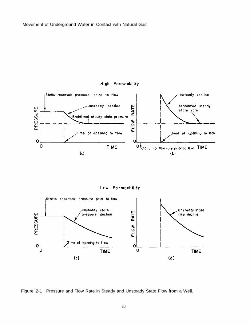
The pressure depletion in a gas or oil reservoir is essentially an unsteady state phenome-
non. If a field, shut-in, at a static, constant pressure throughout, is suddenly opened for produc-
tion, after the unloading of the wells, the pressures and flow rates will immediately begin to drop.
If the permeability of the formation is high, both the pressure at the well and the flow rate may
tend to approach steady state values. In low permeability, tight formations, however, the decline
in both pressure and flow rate will continue for very long periods of time. Figure 2-1 illustrates
the time dependency of rates and pressures in both steady and unsteady state flow. The condition
implied in this figure is a nearby exterior boundary maintained at constant pressure. It may be
noted that in highly permeable reservoirs the steady state values are quickly reached whereas in
tight reservoirs there is no indication of a rapid approach to the steady state conditions. It should
also be noted that the steady state condition is always preceded by unsteady state flow.
Water movement in aquifers is an unsteady state process in that the pressures in the
porous layer and flow rates vary with time. However, there are conditions with water movement
in which a pseudo steady state is reached. For example, in Figure 1-4, after pumping of the water
supply well at a steady rate for a period of a year or more, the pressures in the other wells would
change very slowly. This is the condition which is referred to as pseudo-steady state, Likewise,
water might be entering the water sand through an outcrop or through seepage from above to just
replenish the water being withdrawn, thus maintaining constant pressure at some exterior boundary.
Such a condition would lead to a strictly steady state.
Figure 1-5 illustrates the variation in pressure conditions in an aquifer adjacent to a gas
field pressurized above the aquifer level. It may be seen that the pressure is changing on each
element of water-bearing sand, and that due to the compressibility of the water, the amount of
water leaving each element is not the same as the amount entering the element. This accumulation
by each element of the porous matrix during increasing pressures or depletion during decreasing
pressures must be included in any description of unsteady state flow.
Continuity Equation
The continuity equation expresses the principle of the conservation of mass. When a fluid
is flowing into and out of an element of porous solid, Figure 2-2, the net change in the mass rate
of flow into and out of the element is equal to the rate of change in the mass of fluid in the element.
This change in content in turn can be expressed in terms of the porosity times the change in density
with respect to time. This mass balance on an element is known as the continuity equation:
(2-3)
where
19
Movement of Underground Water in Contact with Natural Gas
Figure 2-1 Pressure and Flow Rate in Steady and Unsteady State Flow from a Well.
20

Figure 2-2 Element of Volume for Derivation of Continuity Equation.
21
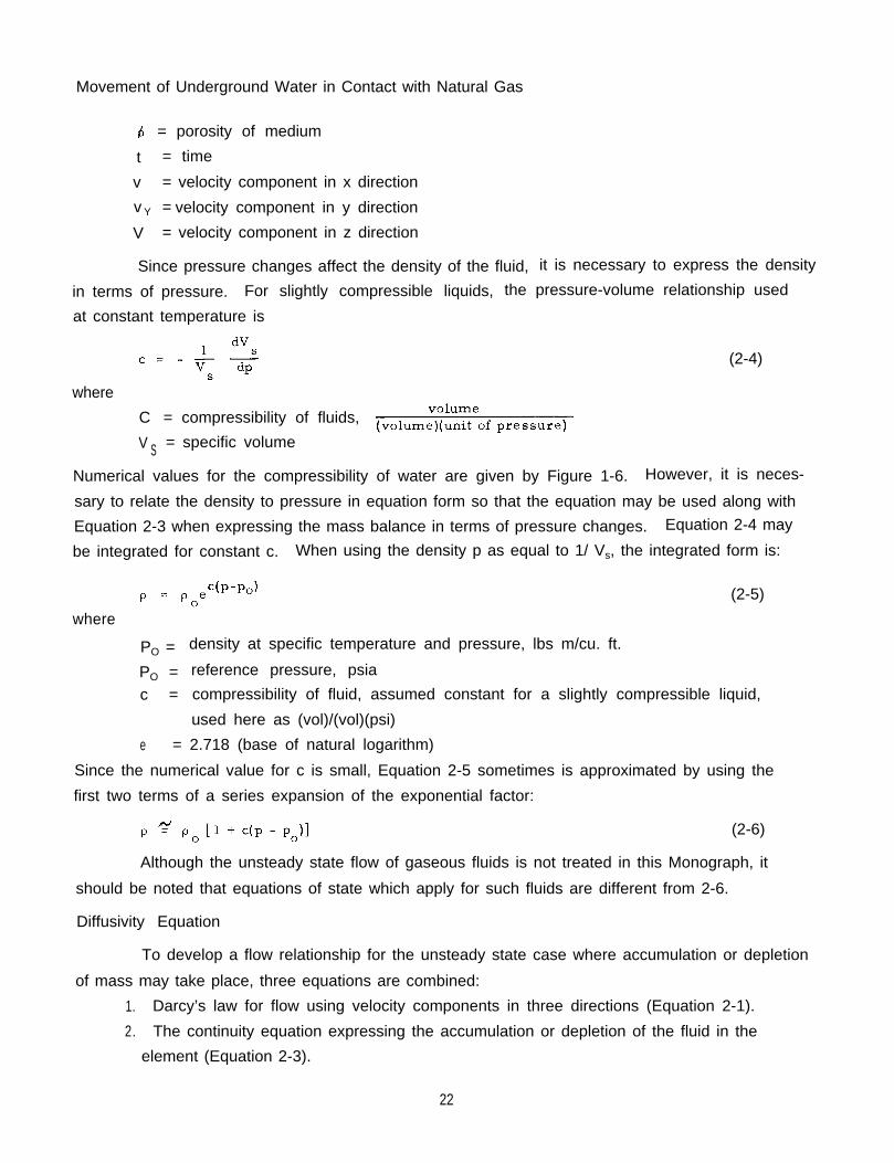
(2-4)
where
C = compressibility of fluids,
V S = specific volume
Numerical values for the compressibility of water are given by Figure 1-6. However, it is neces-
sary to relate the density to pressure in equation form so that the equation may be used along with
Equation 2-3 when expressing the mass balance in terms of pressure changes. Equation 2-4 may
be integrated for constant c. When using the density p as equal to 1/ Vs, the integrated form is:
(2-5)
Movement of Underground Water in Contact with Natural Gas
= porosity of medium
t = time
v = velocity component in x direction
v Y = velocity component in y direction
V = velocity component in z direction
Since pressure changes affect the density of the fluid, it is necessary to express the density
in terms of pressure. For slightly compressible liquids, the pressure-volume relationship used
at constant temperature is
where
PO = density at specific temperature and pressure, lbs m/cu. ft.
PO = reference pressure, psia
c = compressibility of fluid, assumed constant for a slightly compressible liquid,
used here as (vol)/(vol)(psi)
e = 2.718 (base of natural logarithm)
Since the numerical value for c is small, Equation 2-5 sometimes is approximated by using the
first two terms of a series expansion of the exponential factor:
(2-6)
Although the unsteady state flow of gaseous fluids is not treated in this Monograph, it
should be noted that equations of state which apply for such fluids are different from 2-6.
Diffusivity Equation
To develop a flow relationship for the unsteady state case where accumulation or depletion
of mass may take place, three equations are combined:
1. Darcy’s law for flow using velocity components in three directions (Equation 2-1).
2. The continuity equation expressing the accumulation or depletion of the fluid in the
element (Equation 2-3).
22

3. The equation of state expressing the relationship between pressure and density (Equation
2-5).
The diffusivity equation is obtained by combining these three equations, dropping non-linear terms
and neglecting gravity effects.
(2-7)
This diffusivity equation relates pressure, the dependent variable, to position and time,
the independent variables. It is the unsteady state equation for isothermal flow of a slightly com-
pressible liquid through a homogeneous isotropic porous medium. To solve Equation 2-7, it is nec-
essary to specify a geometry for the flow system and impose boundary and initial conditions. This
will be done for the models which may be used to represent the shape of an aquifer adjacent to a
gas storage field, starting with the most widely used case, the radial model.
The Radial Flow Model
Horizontal cylindrical disk shaped geometry is frequently encountered in a large number
of problems related to the movement of water in aquifers. The problem of unsteady-state radial
flow through such a geometry has been solved by Van Everdingen and Hurst (64) who assumed
homogeneous and isotropic properties in the reservoirs.
The geometry of the radial flow model is illustrated in Figure 2-3. The formation thick-
ness is denoted by h, the inner radial boundary by rb and the exterior radial boundary by re. Water
flows in and out of the horizontal aquifer across cylindrical surface of radius rb, and height h. The
extent of the aquifer may be considered infinite or finite at radius r = re. The flow throughout the
aquifer satisfies radial symmetry. The model may be applied to a well completed in a formation
or to a cylindrical gas reservoir surrounded by an aquifer. It is recognized that the gas bubble
does not have the shape of a cylinder but follows the contour of the caprock, Figure 1-5. The
model asserts that the pressure at the cylindrical surface ACBD of Figure 2-3 is the same as that
in the gas bubble.
The assumption on the isotropy of the reservoir properties implies that the permeability
is the same in all directions (e. g., vertical permeability equals horizontal permeability). The
assumption of homogeneity implies on the other hand that the porosity and permeability are the
same regardless of the location in the aquifer. The viscosity and compressibility of the fluid are
assumed constant.
Flow in the radial horizontal model is governed by the diffusivity equation in radial coordi-
nates.
(2-8)
23
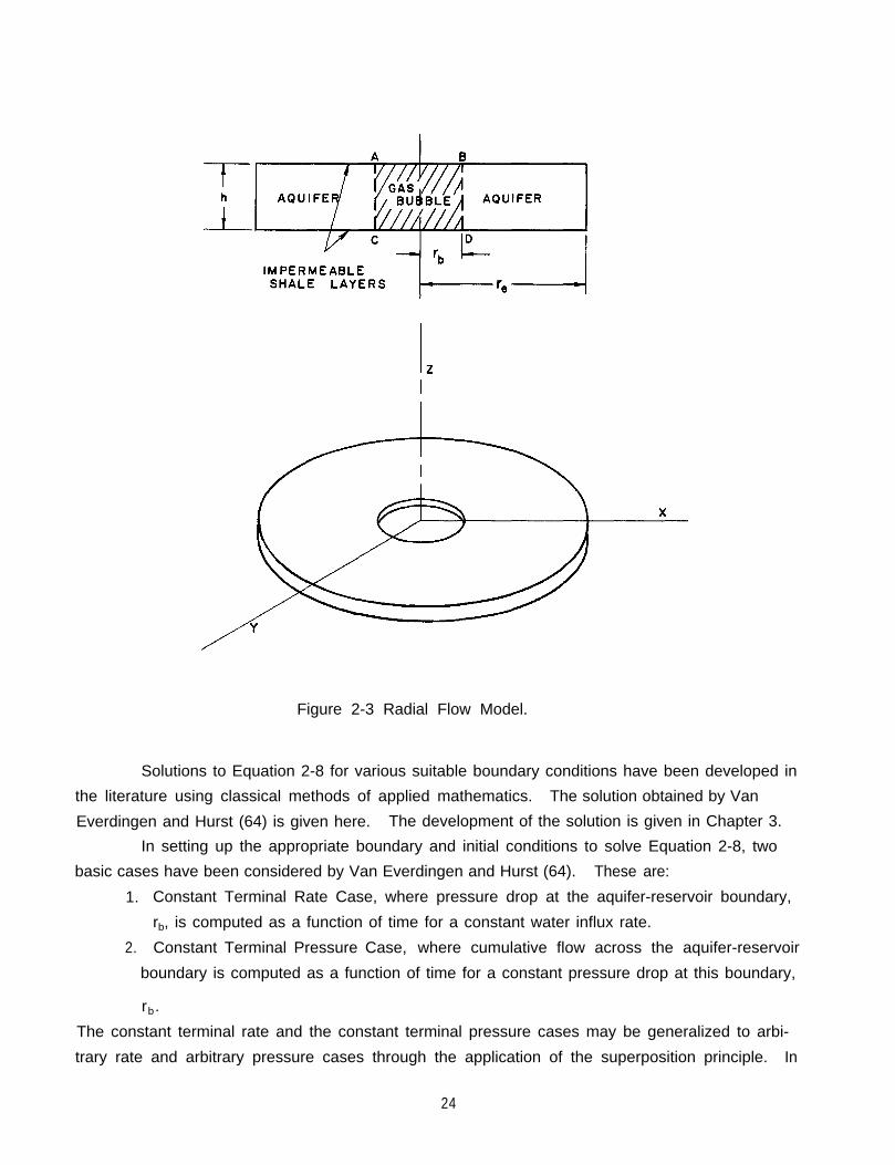
Figure 2-3 Radial Flow Model.
Solutions to Equation 2-8 for various suitable boundary conditions have been developed in
the literature using classical methods of applied mathematics. The solution obtained by Van
Everdingen and Hurst (64) is given here. The development of the solution is given in Chapter 3.
In setting up the appropriate boundary and initial conditions to solve Equation 2-8, two
basic cases have been considered by Van Everdingen and Hurst (64). These are:
1. Constant Terminal Rate Case, where pressure drop at the aquifer-reservoir boundary,
rb, is computed as a function of time for a constant water influx rate.
2. Constant Terminal Pressure Case, where cumulative flow across the aquifer-reservoir
boundary is computed as a function of time for a constant pressure drop at this boundary,
rb.
The constant terminal rate and the constant terminal pressure cases may be generalized to arbi-
trary rate and arbitrary pressure cases through the application of the superposition principle. In
24

applying the superposition principle, the variable pressure or rate specified at the boundary of the
reservoir is treated as a sequence of steps, each of which may be analyzed using solutions of the
rate or constant terminal pressure cases. Application of the superposition principle will be dis-
cussed in Chapter 5.
The Rate Case
The boundary and initial conditions for the constant terminal rate case are:
1. There is no pressure gradient and hence no flow at the exterior boundary of the aquifer,
Ie .
2. The pressure gradient in the radial direction at the gas-water contact rb is constant,
implying constant flow.
3. The initial pressure throughout the aquifer is constant.
The working equation for the constant rate case is given by Equation 2-9 (64).
(2-9)
where, in field units
PO = equilibrium or discovery reservoir pressure, psia
P = reservoir pressure at inner boundary of aquifer (rb ) at time t, psia
ew = water influx rate, cubic feet per day (for barrels per day, 25. 15 becomes 141. 2)
K = aquifer permeability, millidarcys
h = aquifer thickness, feet
f = fraction of circle open to flow in case full radial model does not apply. Equals
unity for full radial model.
Pt = dimensionless pressure drop for constant terminal rate case as obtained from
tables and dimensionless time, tD
(2-10)
t = time, days
µ = viscosity of water in aquifer, centipoise
c = composite compressibility of porous formation containing water, (vol)/(vol)(psi)
r b = radius of inner boundary, feet
= fractional porosity
The tables of Pt functions published by Van Everdingen and Hurst (64) have been augmented
by Chatas (5) and in this research (37). Tables of Pt are given for infinite aquifers in Appendix A,
for limited aquifers with no flow across the exterior boundary as a function of re/rb in Appendix C,
25

Movement of Underground Water in Contact with Natural Gas
and for limited aquifers with a constant pressure at the exterior boundary as a function of r e / r b
in Appendix E.
The use of dimensionless terms is convenient in the solution of partial differential equa-
tions. Dimensionless time values depend not only upon real time, but also the other variables.
Dimensionless groups are convenient in that any consistent set of units may be used for the terms
comprising a group. An example calculation will illustrate the simplicity of the constant rate
case for unsteady state calculations.
Example Problem No. 2-1
Starting with a uniform aquifer pressure of 700 pounds per square inch absolute, it is
desired to grow a storage reservoir at a constant rate of 50,000 cubic feet pore volume per day.Calculate the reservoir pressure at 30, 60, 120, 180, and 300 days after initiation of gas bubble.
Assume the aquifer to be infinite in extent and that its performance can be approximated by the
radial model.
The following data are available on physical and geometric properties of the gas bubble-
aquifer system.
P O = initial pressure, 700 psia
h = thickness, 80 feet
r b = bubble radius, 1000 feet
K = permeability, 400 millidarcys
compressibility, 7 x 10⁻⁶c = vol/(vol)(psi)
m = porosity, 0.17
µ = viscosity, 1 centipoise
Solution
Using t as time in days the dimensionless time value is calculated using Equation 2-10.
Dimensionless pressure values, Pt, for the infinite radial model, constant terminal rate case,
corresponding to dimensionless time are obtained from Appendix A. Equation 2-9 is used to
obtain the reservoir pressure.
26

Table 2-1 Pressure and Time Values for Example Problem No. 2-1
It may be noted that the rate of pressure rise over and above the initial aquifer value
decreases with time for a constant rate of water efflux.*
The Pressure Case
The constant terminal pressure case gives the cumulative water influx passing the reser-
voir boundary over a time period t caused by a constant pressure drop at that boundary. It is
obtained by solving the diffusivity equation expressed in the radial coordinate system (Equation 2-8)
with the following initial and boundary conditions:
1. The initial pressure throughout the aquifer is constant.
2. There is no pressure gradient and hence no flow at the exterior boundary of the aquifer,re.
3. The pressure drop at the gas-water interface is constant.
As in the constant terminal rate case, the ratio of the exterior radius to the gas bubble
radius, re/rb = R, may be finite or infinite and the solution for dimensionless cumulative water
influx, Qt’ will depend upon the boundary condition chosen.
The working equation satisfying the above conditions for the constant terminal pressure
case is given as follows:
(2-11)
where
w =e cumulative water influx, cubic feet
po-p = initial pressure minus prevailing pressure at rb, psi
Q t = dimensionless cumulative water influx, obtained from tables and tD defined as in
Equation 2-10.
Qt values are given in Appendix B for the infinite aquifer and in Appendix D for the limited
aquifer with no flow across the exterior boundary.
* The terms “influx” and “efflux” should not be confused. As used in this text, the water flow isalways taken with respect to the gas bubble. Hence efflux refers to water flowing from the gasbubble into the aquifer.
27

Movement of Underground Water in Contact with Natural Gas
Example Problem No. 2-2
A natural gas producing reservoir had an original discovery pressure of 700 pounds per
square inch absolute. The gas reservoir is roughly circular in shape, horizontal and is in contact
with an aquifer which may be considered infinitely large. The thickness of the aquifer is 30 feet.
For the first three months of gas production, the pressure in the gas bubble is to be maintained
at 690 pounds per square inch absolute. It is desired to calculate the cumulative water influx into
the gas sand during the first three months of gas production after discovery. The radius of the
gas field or the inner boundary of the aquifer is rb = 5000 feet. The compressibility of the aquifer
is c = 7x10 -6 (vol)/(vol)(psi).
The permeability of the aquifer sand is K = 100 millidarcys. The porosity is 15 per cent.
The viscosity of the water in the aquifer is one centipoise.
Solution
Using equation 2-11
Qt is a function of the dimensionless time t D which is given in Equation 2-10.
= 127,500 cubic feet cumulative water influx into gas bubble during the three months.
It should be noted that Equations 2-9 and 2-11 apply equally well to the infinite and limited
aquifer cases provided the Pt and Qt functions are obtained from the appropriate table.
Steady State Flow
Since flow adjacent to the inner aquifer boundary may approach steady state conditions on
certain occasions, the steady state equation for a horizontal laminar flow of liquids is given:
(2-12)
28

where
e w = liquid flow rate, cubic feet per day (The conversion factor 0.03976 becomes
0.007087 for flow rate in barrels per day. )
h = formation thickness, feet
K = permeability, millidarcys
P = pressure, psia
µ = liquid viscosity, centipoises
r = radius, feet
It is customary to consider flow as taking place from point 1; i. e., r1 and p1, toward
point 2; i. e., r2 and p2. Equation 2-12 above tacitly assumes that the well or the radial inner
boundary fully penetrates the entire thickness, h, of the formation.
The Linear Flow Model
Figure 2-4 shows a linear model where the flow takes place only between the end faces
abdc and fgkh; i. e., the other four surfaces are impervious to flow. The case of the linear model
used here, Figure 2-5, is one in which the flow into or out of the water filled porous solid takes
place only through one face, ABCD, with the other end either closed by a barrier or considered
infinite in extent. The linear model applies to reservoirs which are bounded by impermeable zones
such as two parallel faults which place shale opposite sand on faces afhc and bgkd of Figure 2-4.
The diffusivity equation for a linear system is
(2-13)
Solutions to this equation are obtained by applying conditions of constant terminal rate and
constant terminal pressure as used with the radial model.
The Rate Case
The rate case is presented first; the rate is specified at the interior boundary ABCD and
the solution relates pressure to time. The initial and boundary conditions for the constant-terminal
rate case are:
1. The pressure is uniform throughout the aquifer at the initial time.
2. The aquifer is infinite in linear extent.
3. Production starts at zero time and remains constant thereafter.
With these conditions, the following equation is derived:
(2-14)
29
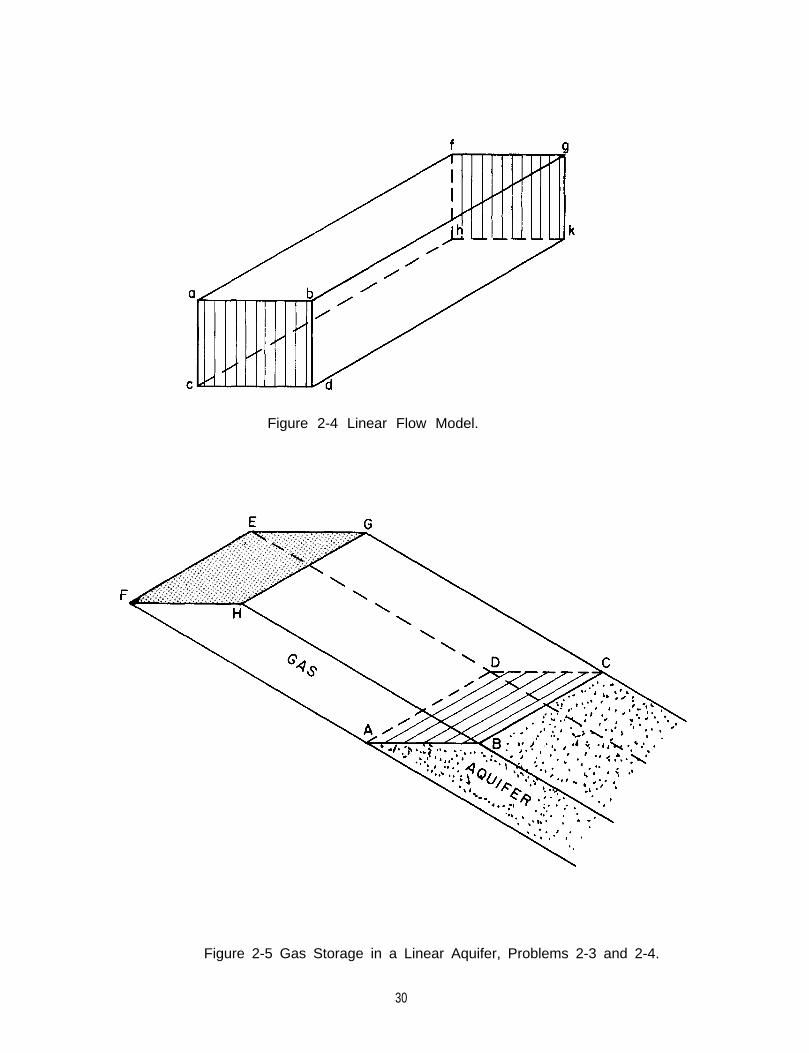
Figure 2-4 Linear Flow Model.
Figure 2-5 Gas Storage in a Linear Aquifer, Problems 2-3 and 2-4.
30

where
P = pressure at face where rate is specified, psia
PO = initial pressure, psia
e w = fluid influx rate, cubic feet per day
µ = fluid viscosity, centipoise
A = cross sectional area to flow, square feet
K = permeability, millidarcys
θ = transformed time =
t = time, days
= fractional porosity
c = fluid compressibility vol/(vol)(psi)
Example Problem No. 2-3
It is desired to grow a gas bubble on an aquifer extending indefinitely in one direction and
located between two parallel faults at the rate of 100 cubic feet per day, Figure 2-5. Determine
the gas reservoir pressure at 30, 60, 90, and 365 days after initiation of the gas bubble.
The available data on the physical and geometric properties of the gas bubble-aquifer
system are given below.
P O = initial aquifer pressure, 400 psia
K = permeability, 300 millidarcys
C = compressibility, 7 x 10⁻⁶ vol/(vol)(psi)
= porosity, 0.16
µ = viscosity, 1 centipoise
A = area of cross section of aquifer, ABCD, Figure 2-5, 20,000 feet2 *
Solution
At t = 30 days, the pressure is calculated from Equation 2-14.
Similarlyfor 60 days p = 400 t 29.8 = 429.8 psia
for 90 days p = 400 t 36.6 = 436.6 psia
for 365 days p = 400 t 73.7 = 473.7 psia
*The area used should always be the cross sectional area; i. e.,linear flow and not necessarily the gas water contact area.
perpendicular to the direction of
31

Movement of Underground Water in Contact with Natural Gas
The Limited Linear Case at constant rate has been treated recently in the literature.
Mueller (43a) has provided solutions for limited aquifers of constant width. He included a factor
β = ho/hi which permits handling cases of tapered thickness, Figure 2-6. The equation for com-
puting the pressures at the inflow face is:
(2-14a)
where L = length of aquifer, feet
The value of Pt is found from Figure 2-7 with the proper value of β = ho/hi, the ratio of the height
at the closed outer boundary to the height of the inner boundary as a function of dimensionless time, tD
Mueller (43a) has also investigated the cases were permeability, reciprocal viscosity,
compressibility, or porosity vary linearly inside the aquifer.
Figure 2-6 Limited Linear Model of Constant Width and Tapered Thickness.
32

33
Movement of Underground Water in Contact with Natural Gas
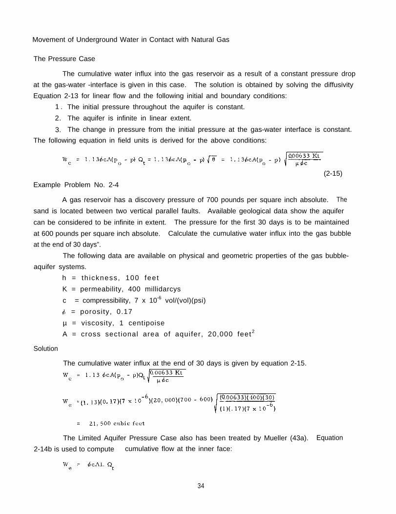
The Pressure Case
The cumulative water influx into the gas reservoir as a result of a constant pressure drop
at the gas-water -interface is given in this case. The solution is obtained by solving the diffusivity
Equation 2-13 for linear flow and the following initial and boundary conditions:
1 . The initial pressure throughout the aquifer is constant.
2. The aquifer is infinite in linear extent.
3. The change in pressure from the initial pressure at the gas-water interface is constant.
The following equation in field units is derived for the above conditions:
Example Problem No. 2-4
(2-15)
A gas reservoir has a discovery pressure of 700 pounds per square inch absolute. The
sand is located between two vertical parallel faults. Available geological data show the aquifer
can be considered to be infinite in extent. The pressure for the first 30 days is to be maintained
at 600 pounds per square inch absolute. Calculate the cumulative water influx into the gas bubble
at the end of 30 days”.
The following data are available on physical and geometric properties of the gas bubble-
aquifer systems.
h = th ickness, 100 feet
K = permeability, 400 millidarcys
compressibility, 7 x 10⁻⁶ c = vol/(vol)(psi)
= porosity, 0.17
µ = viscosity, 1 centipoise
A = cross sectional area of aquifer, 20,000 feet 2
Solution
The cumulative water influx at the end of 30 days is given by equation 2-15.
The Limited Aquifer Pressure Case also has been treated by Mueller (43a). Equation
2-14b is used to compute cumulative flow at the inner face:
34
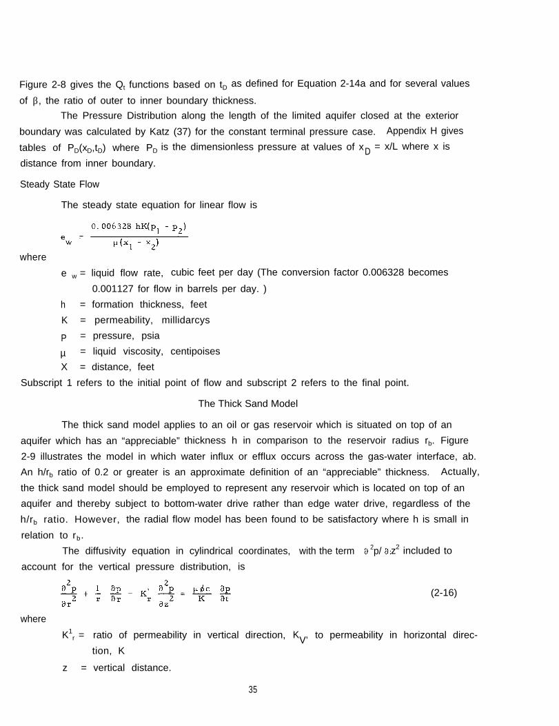
Figure 2-8 gives the Qt functions based on tD as defined for Equation 2-14a and for several values
of β, the ratio of outer to inner boundary thickness.The Pressure Distribution along the length of the limited aquifer closed at the exterior
boundary was calculated by Katz (37) for the constant terminal pressure case. Appendix H gives
tables of PD(xD,tD) where PD is the dimensionless pressure at values of xD = x/L where x is
distance from inner boundary.
Steady State Flow
The steady state equation for linear flow is
where
e w = liquid flow rate, cubic feet per day (The conversion factor 0.006328 becomes
0.001127 for flow in barrels per day. )
h = formation thickness, feet
K = permeability, millidarcys
P = pressure, psia
µ = liquid viscosity, centipoises
X = distance, feet
Subscript 1 refers to the initial point of flow and subscript 2 refers to the final point.
The Thick Sand Model
The thick sand model applies to an oil or gas reservoir which is situated on top of an
aquifer which has an “appreciable” thickness h in comparison to the reservoir radius rb. Figure
2-9 illustrates the model in which water influx or efflux occurs across the gas-water interface, ab.
An h/rb ratio of 0.2 or greater is an approximate definition of an “appreciable” thickness. Actually,
the thick sand model should be employed to represent any reservoir which is located on top of an
aquifer and thereby subject to bottom-water drive rather than edge water drive, regardless of the
h/rb ratio. However, the radial flow model has been found to be satisfactory where h is small in
relation to rb.
The diffusivity equation in cylindrical
account for the vertical pressure distribution,
where
coordinates, with the term 2p/ z2 included to
is
(2-16)
K1r = ratio of permeability in vertical direction, KV’ to permeability in horizontal direc-
tion, K
z = vertical distance.
35

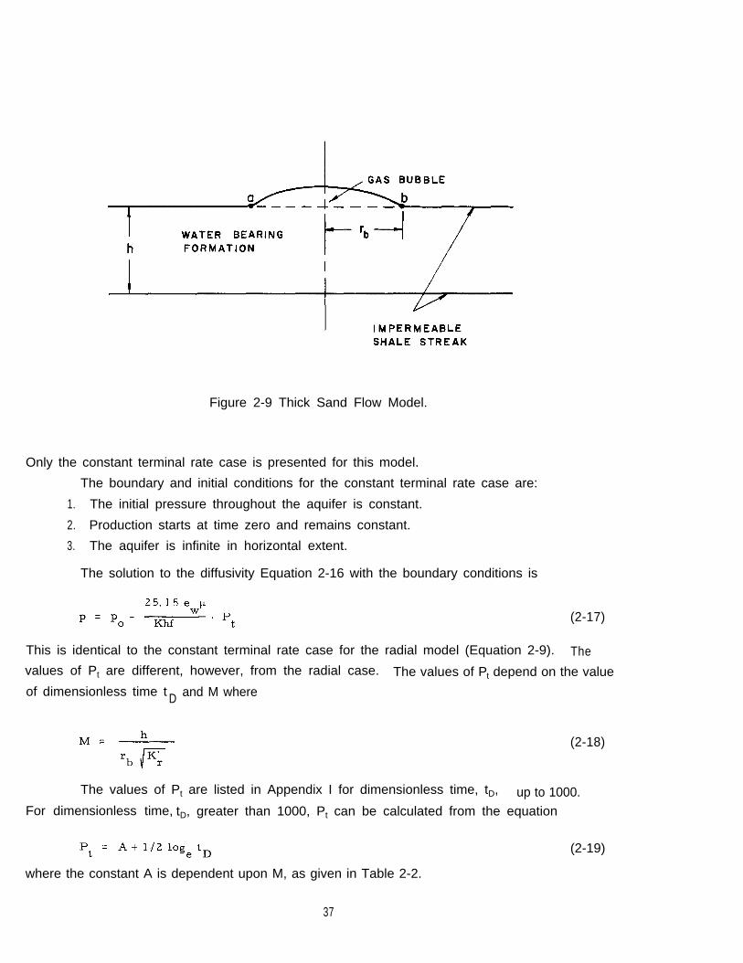
Figure 2-9 Thick Sand Flow Model.
Only the constant terminal rate case is presented for this model.
The boundary and initial conditions for the constant terminal rate case are:
1. The initial pressure throughout the aquifer is constant.
2. Production starts at time zero and remains constant.
3. The aquifer is infinite in horizontal extent.
The solution to the diffusivity Equation 2-16 with the boundary conditions is
(2-17)
This is identical to the constant terminal rate case for the radial model (Equation 2-9). Thevalues of Pt are different, however, from the radial case. The values of Pt depend on the valueof dimensionless time t D and M where
(2-18)
The values of Pt are listed in Appendix I for dimensionless time, tD, up to 1000.For dimensionless time, tD, greater than 1000, Pt can be calculated from the equation
where the constant A is dependent upon M, as given in Table 2-2.
(2-19)
37

Movement of Underground Water in Contact with Natural Gas
Table 2-2 Parameter A as a Function of M for the Thick Sand Model
It is interesting to compare pressure drops given by the thick sand model with those from
the radial model. The radial model is strictly valid for reservoirs in thin aquifers subject to edge
water drive only, whereas the thick sand model applies to reservoirs with bottom water drive. The
ratio, R, of the pressure drop calculated from the thick sand model to pressure drops for the radial
model is plotted in Figure 2-10 as a function of dimensionless time t D with M as parameter. For
M less than 0.5 the pressure drop calculated by the radial flow model equation is greater than the
actual drop for small time and less than the actual drop for large time. For M greater than 0.5,
the radial flow model yields pressure drops greater than actual for all time. The error incurred
by use of the radial model is seen to be less as M is smaller; i. e., as the aquifer thickness is
smaller in relation to rb. The use of the thick sand model is recommended for values of h/rb
greater than 0.2.
Example Problem No. 2-5
A newly discovered gas reservoir is situated on an aquifer formation approximately 380
feet thick. Calculate the reservoir pressure at 90, 180, and 270 days after discovery if the water
encroachment rate is approximately one million cubic feet per week. The discovery pressure is
600 psia.
The following data are known or estimated:
K = permeability, 199 millidarcys (horizontal)
µ = viscosity, 1 centipoise
rb = gas bubble radius, 6,000 feet
C = compressibility, 7 x 10⁻⁶vol/(vol)(psi)
= porosity, 0.15
Kr = permeability ratio, 0.4
For constant water influx, Equation 2-17 is used.
38


Movement of Underground Water in Contact with Natural Gas
p = 600 - 47.5 Pt
at t = 90 days, tD =0.0333(90) = 3
at t = 180 days, tD = 6
at t = 270 days, tD = 9
From Appendix I,
P t( tD = 3) = 1.2490
P t( tD = 6) = 1.5770
P t( tD = 9) = 1.7732
Thus
P90 = 600 - 47.5(1. 2490) = 600 - 59 = 541 psia
P180 = 600 - 47.5(1. 5770) = 600 - 75 = 525 psia
P270 = 600 - 47.5(1. 7732) = 600 - 84 = 516 psia
Hemispherical Flow Model
For very thick aquifers we can assume the aquifer infinite in both the horizontal and vertical
direct ions and treat the water flow as spherically radial. The gas bubble is then considered as the
inner hemispherical boundary and the outer boundary is considered at infinity for the aquifer-water
flow system. Figure 2-11 is a sketch of the hemispherical flow model showing the assumed circular
areal geometry and the reservoir radius rb.
The diffusivity equation governing spherical, unsteady-state flow of a compressible liquid
through a porous medium is
(2-20)
where
z = vertical distance
y = the specific weight of water in pounds force/ft3 =pg/gc
g = acceleration due to gravity
gc= standard acceleration due to gravity
(Note: g/gc normally equals 1.0 lb force/lb mass)
40

Figure 2-11 Hemispherical Flow Model.
The Rate Case
The boundary and initial conditions for the constant terminal rate case are
1. The initial pressure throughout the aquifer is constant.
2. Production starts at time zero and remains constant.
3. The aquifer is infinite in vertical and lateral extent.
The solution to these boundary and initial conditions and the diffusivity Equation 2-20 is
41

Movement of Underground Water in Contact with Natural Gas
where erf is the error function,
Values of erf (x) are tabulated in the literature (30).
Example Problem No. 2-6
(2-21)
A newly discovered gas field is situated on an aquifer having the following estimated
properties:
PO = initial pressure, 400 psia
K = permeability, 266 millidarcys
µ = viscosity, 1 centipoise
C = compressibility, 7 x 10⁻⁶vol/(vol)(psi)
= porosity, 0.15
r b = gas bubble radius, 6,000 ft
Since geological data indicate no continuous, impermeable shale streak in the first 5,000 feet
below the reservoir, the hemispherical model can be used to estimate the aquifer behavior. Gas
is removed causing water influx at the rate of one million cubic feet per day. Calculate the pres-
sure in the gas bubble after 90 days.
Solution
Use Equation 2-21 to calculate the pressure
From page 24 of Jahnke and Emde (30)
and
Thus
42
p = 400 - 31.5 (1 -0.275)
p = 377.2 psia
The Pressure CaseThe boundary and initial conditions for the constant terminal pressure case are
1. The initial pressure throughout the aquifer is constant.
2. A pressure drop occurs at time zero and remains constant.
3. The aquifer is infinite in lateral and vertical extent.
The solutions to these conditions along with the diffusivity Equation 2-20 is
(2-22)
Example Problem No. 2-7
Using the data given in example problem no. 6, estimate the cumulative water influx
after 90 days for a constant pressure drop of 100 psi in the gas bubble
Solution
From example problem no. 2-6, tD = 4
Using Equation 2-22
Elliptical Flow Model
The elliptical flow model is similar to the horizontal radial flow model treated by Van
Everdingen and Hurst (64) in that the aquifer formation thickness is assumed small and vertical
flow effects are assumed negligible. However, the areal boundary of the gas bubble is taken as
an ellipse rather than a circle. Many actual gas and oil fields conform more closely to
ellipses of appropriate eccentricity than to circles. The elliptical model was investigated pri-
marily to determine the degree of error involved in assuming circular geometry.
Figure 2-12 shows a sketch of the elliptical model and the relationship between the
Cartesian coordinates x and y and the elliptic planar coordinates u and v. The condition u =
constant specifies an ellipse and v = constant specifies an hyperbola, as shown in the figure.
The value of the constant determines which ellipse or which hyperbola is specified.
The diffusivity equation expressed in elliptic coordinates is:
43

Figure 2-12 Elliptical Flow Model.
(2-23)
wheretD = dimensionless time for elliptic flow =
= focal length of the ellipse (see Figure 2-12).
Equation 2-23 has been solved numerically for the constant terminal pressure case for
the same initial and boundary conditions as the radial model (7). Dimensionless influx quantities,
Qt were calculated. These are related to the actual cumulative water influx by
where ∆ p is the (constant) pressure drop at the gas bubble boundary. Qt is tabulated as a function
of dimensionless time t D in Table 2-3 for an ellipse with eccentricity of 0.925 or a ratio of 2.63
between major and minor axes. The exterior radius was taken as the confocal ellipse on which
44

Table 2-3 Dimensionless Water Influx vs Dimensionless Time for Elliptical Flow Model.
u = ue = 2.6. The aquifer was limited in extent; it had an area equal to 100 times the bubble
area.
Table 2-3 represents but one of an infinite number of combinations of eccentricity and
ratios of exterior to interior radii.
Studies performed on the elliptical model have shown that the error incurred by applying
radial flow calculations to elliptically shaped reservoirs is inversely proportional to the magnitude
of the dimensionless time values employed in the calculations. That is, the major error occursat low values of dimensionless time. Analysis of this initial period in actual field operations is
often complicated by such problems as a moving gas-water interface, pressure gradients in the
gas bubble, etc. Due to the uncertainty of data during this period, the success of radial flow
calculations, and to the large number of tables required to describe all the combinations possible
for the elliptic geometry, further numerical computations of the dimensionless values for the
elliptical flow model were not made. For further information on this model, the reader is
referred to Reference 7.
Comparison of Dimensionless Functions
The values of Pt, the dimensionless pressure at the gas-water boundary, and of Qt,
the dimensionless influx rate, are plotted on Figures 2-13 and 2-14, respectively.
45

Figure 2-13 Comparison of Dimensionless Pressure Functions, Pt, for Various Models
46

Figure 2-14 Comparison of Dimensionless Water Influx, Qt, for Various Models
47

This Page Intentionally Left Blank
CHAPTER 3
DERIVATIONS OF FLOW EQUATIONS FOR MODELS
This chapter presents the derivation of the flow equations for various geometric models.
In Chapter 2, the working equations are presented for the practicing engineer with a minimum of
mathematical development so that readers who are interested only in applications can avoid the
complex mathematical concepts needed to solve the diffusivity equations. Since the derivations
usually involve such mathematical topics as Laplace Transform, Bessel functions, and partial
differential equations, they have been reserved to this chapter for more detailed treatment.
The derivation of the flow equations should be valuable to those who wish to make further
developments in unsteady state flow. The models treated in this chapter are:
1. Radial model, constant terminal rate -- infinite aquifer
2. Radial model, constant terminal pressure -- infinite aquifer
3. Radial model, constant terminal rate -- finite aquifer
4. Radial model, constant terminal pressure -- finite aquifer
5. Linear model, constant terminal rate -- infinite aquifer
6. Linear model, constant terminal pressure -- infinite aquifer
7. Thick Sand model, constant terminal rate -- infinite aquifer
8. Hemispherical model, constant terminal pressure -- infinite aquifer
9. Elliptical model, constant terminal pressure -- infinite aquifer
The nature of the geometric models is illustrated by the appropriate figures in Chapter 2.
Radial Model (Constant Terminal Rate Case, Infinite Aquifer)
The unsteady state radial flow of a liquid through a horizontal disk shape model was
represented for constant terminal rate by the working Equation 2-9 in the preceding chapter. This
equation was obtained by solving the diffusivity equation:
where is the Laplacian operator in polar coordinates with axial symmetry:
for the initial and boundary conditions
(3-1)
(3-2)
(3-3)
(3-4)
(3-5)
49
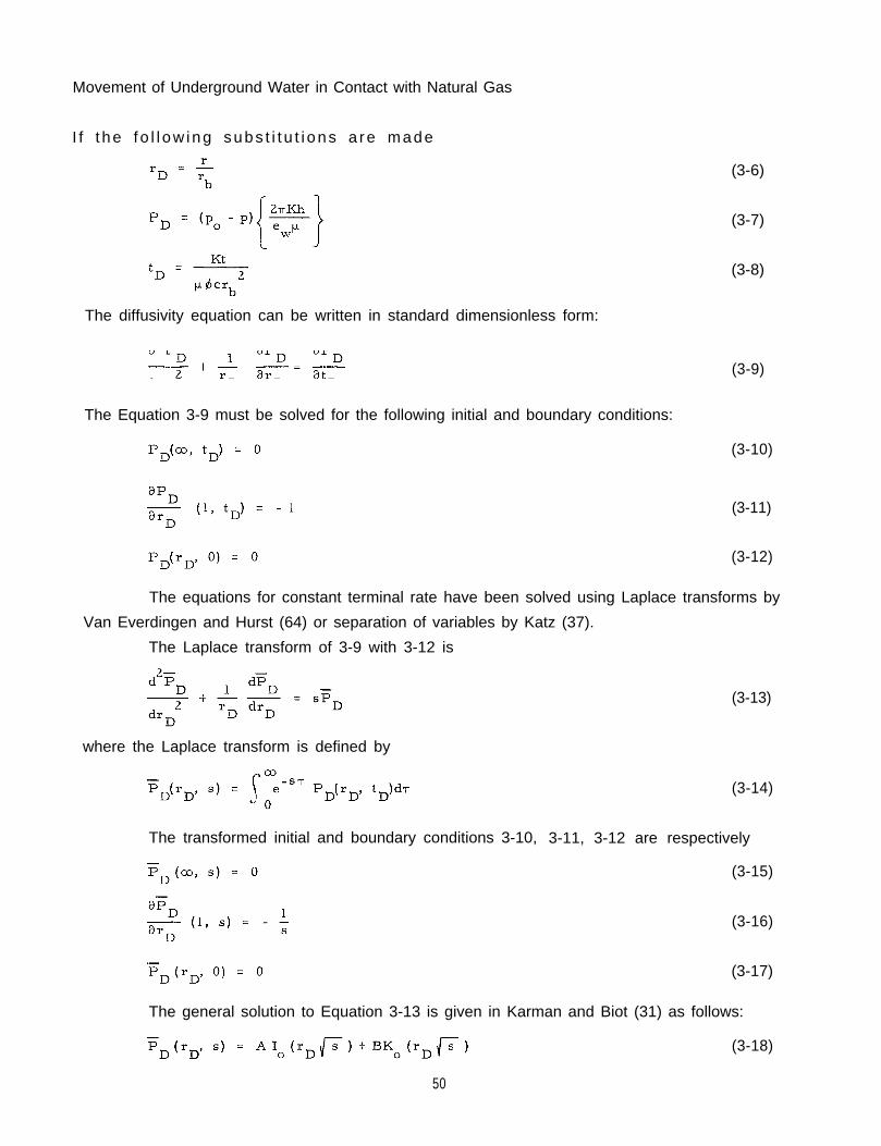
Movement of Underground Water in Contact with Natural Gas
I f t he f o l l ow ing subs t i t u t i ons a re made
The diffusivity equation can be written in standard dimensionless form:
The Equation 3-9 must be solved for the following initial and boundary conditions:
(3-6)
(3-7)
(3-8)
(3-9)
(3-10)
(3-11)
(3-12)
The equations for constant terminal rate have been solved using Laplace transforms by
Van Everdingen and Hurst (64) or separation of variables by Katz (37).
The Laplace transform of 3-9 with 3-12 is
(3-13)
where the Laplace transform is defined by
(3-14)
The transformed initial and boundary conditions 3-10, 3-11, 3-12 are respectively
(3-15)
(3-16)
(3-17)
The general solution to Equation 3-13 is given in Karman and Biot (31) as follows:
(3-18)
50

where A and B are constants of integration, and Io and Ko are Bessell functions of zero order
first and second kind. Since PD(rD,s) must vanish as rD goes to infinity, the value of A is
zero and Equation 3-18 becomes
Differentiation of Equation 3-19 yields, at rD = 1
(3-19)
(3-20)
Comparison of Equation 3-16 and Equation 3-20 shows that
(3-21)
Substitution of Equation 3-21 in Equation 3-19 gives the Laplace transform for the dimensionless
pressure drop for the constant terminal rate case, infinite aquifer:
(3-22)
Van Everdingen and Hurst (64) show that the inverse of Equation 3-22 is
(3-23)
In order to obtain dimensionless pressure drop, PD, at the bubble edge, we substitute rD = 1
and note that:
(3-24)
in Equation 3 - 23. Thus
(3-25)
Equation 3-25 was solved by numerical methods. The table of dimensionless pressure drop Pt,
at the boundary, as a function of dimensionless time, t D’ is presented in Appendix A. Tables of
the dimensionless pressure distribution, P (rD D, tD), as a function of dimensionless time, t D a r e
given in Appendix G.
The pressure at the bubble edge can be calculated from Equation 2-9 by
(3-26)
51

Movement of Underground Water in Contact with Natural Gas
Equation 3-26 expressed in field units is
(2-9)
where p is the pressure at rb , the gas-aquifer boundary.
In order to calculate p at a radial position other than the boundary, using Appendix G,
one employs the equation
where p is now the pressure at radius r = rbrd
(3-27)
Radial Model (Constant Terminal Pressure Case, Infinite Aquifer)
Equation 2-11 describing the unsteady-state flow of slightly compressible fluids for radial
flow for constant terminal pressure was obtained by solving the diffusivity equation
for the initial and boundary conditions:
If the following substitutions
are made in Equations 3-2, 3-3, 3-27, 3-5 the resulting diffusivity equation
must be solved for the initial and boundary conditions:
(3-2)
(3-3)
(3-27)
(3-5)
(3-6)
(3-28)
(3-8)
(3-29)
52
(3-30)
(3-31)
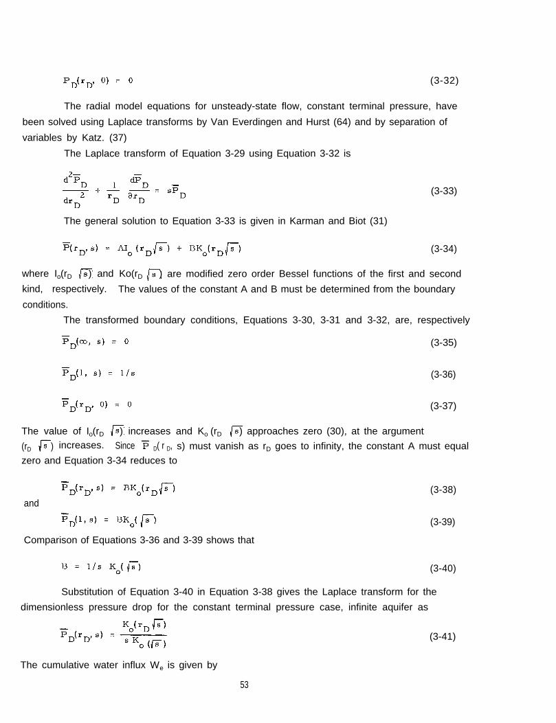
(3-32)
The radial model equations for unsteady-state flow, constant terminal pressure, have
been solved using Laplace transforms by Van Everdingen and Hurst (64) and by separation of
variables by Katz. (37)
The Laplace transform of Equation 3-29 using Equation 3-32 is
The general solution to Equation 3-33 is given in Karman and Biot (31)
(3-33)
(3-34)
where Io(rD ) and Ko(rD ) are modified zero order Bessel functions of the first and second
kind, respectively. The values of the constant A and B must be determined from the boundary
conditions.
The transformed boundary conditions, Equations 3-30, 3-31 and 3-32, are, respectively
(3-35)
(3-36)
(3-37)
The value of Io(rD ) increases and Ko (rD ) approaches zero (30), at the argument
(rD ) increases. Since D( r D, s) must vanish as rD goes to infinity, the constant A must equalzero and Equation 3-34 reduces to
and
Comparison of Equations 3-36 and 3-39 shows that
(3-38)
(3-39)
(3-40)
Substitution of Equation 3-40 in Equation 3-38 gives the Laplace transform for the
dimensionless pressure drop for the constant terminal pressure case, infinite aquifer as
(3-41)
The cumulative water influx We is given by
53

Movement of Undereround Water in Contact with Natural Gas
or equivalently
where
(3-41 a)
(3-41b)
(3-42)
and ∆ p -po, - p1 = pressure drop at the gas aquifer boundary.
The Laplace transform of Equation 3-42 is
(3-43)
and substituting Equation 3-41 into Equation 3-43
(3-43a)
The inverse of this expression, given by Van Everdingen and Hurst (64) is
(3-44)
Values of the dimensionless cumulative water influx, Qt, as a function of dimensionless
time, tD, were obtained by integrating the Equation 3-44 by numerical methods (5)(37)( 64). Tables
of these values are presented in Appendix B.
Values of [ 1 - PD(rD, tD)] have been obtained by the method of separation of variables
by Katz (37). Values are tabulated in Appendix G. The actual pressure p at a position r = rbrD
and time tD is calculated from
Although a finite aquifer was employed to facilitate the calculation of 1 - PD(rD,tD)(Appendix G),
the results can be used for infinite aquifers provided certain rules are observed as illustrated in
Example Problem 7-3.
Radial Model (Constant Terminal Rate Case. Finite Aquifer)
The dimensionless pressure distribution is found by solving the diffusivity equation
54

(3-13)
where PD is given by Equation 3-7. The initial and boundary conditions are
(3-46)
(3-11)
(3-14)
where R =
Following the procedures in the previous derivations, one finds the Laplace transform
of the dimensionless pressure PD(rD,tD) to be
The inverse of Equation 3-47 is given by Van Everdingen and Hurst (64) as
where β n, are the roots of
(3-49)
For rD = 1, the pressure at the bubble edge can be calculated by
(3-47)
(3-48)
(3-50)
55
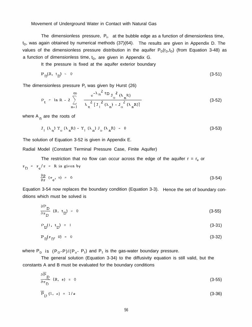
Movement of Underground Water in Contact with Natural Gas
The dimensionless pressure, Pt, at the bubble edge as a function of dimensionless time,
tD, was again obtained by numerical methods (37)(64). The results are given in Appendix D. The
values of the dimensionless pressure distribution in the aquifer PD(rD,tD) (from Equation 3-48) as
a function of dimensionless time, tD, are given in Appendix G.
It the pressure is fixed at the aquifer exterior boundary
The dimensionless pressure Pt was given by Hurst (26)
where A are the roots ofn
The solution of Equation 3-52 is given in Appendix E.
Radial Model (Constant Terminal Pressure Case, Finite Aquifer)
The restriction that no flow can occur across the edge of the aquifer r = re or
(3-51)
(3-52)
(3-53)
(3-54)
Equation 3-54 now replaces the boundary condition (Equation 3-3). Hence the set of boundary con-
ditions which must be solved is
(3-55)
(3-31)
(3-32)
where PD i s (PO -P) / (P o- P1) and P1 is the gas-water boundary pressure.
The general solution (Equation 3-34) to the diffusivity equation is still valid, but the
constants A and B must be evaluated for the boundary conditions
(3-55)
(3-36)
56

Thus the transformation of the boundary condition at rD = 1 is
(3-56)
(3-57)
Solving Equation 3-56 and 3 -57 for A and B gives
and
(3-58)
(3-59)
Substitution of these constants into the general solution (Equation 3-34) yields
Thus the transform of the dimensionless water influx Equation 3-43 is given by:
The inverse of this equation is given by Van Everdingen and Hurst (64) as
(3-60)
(3-61)
(3-62)
where n are the roots of
(3-63)
The dimensionless water influx, Qt, was numerically evaluated as a function of dimension-
less time, tD, and the ratio R of the aquifer exterior radius to the gas bubble radius. These tables
are given in Appendix C.
The values of dimensionless pressure, PD(rn, tD) for the dimensionless pressure distri-
bution in the aquifer are given in the form 1 - PD(rD,tD) in Appendix F.
Linear Model (Constant Terminal Rate Case)
The derivation of the working Equation 2-14 for the linear flow model, rate case is pre-
sented below. The diffusivity equation governing one- dimensional, unsteady-state flow of a liquid
through porous media is
57

Movement of Underground Water in Contact with Natural Gas
Definition of the new variables
where po is the initial aquifer pressure, allows Equation 3-64 to be written as follows:
The initial and boundary conditions for the constant-rate case are
(3-64)
(3-65)
(3-66)
(3-67)
(3-68)
(3-69)(3-70)
(3-71)
where e is the constant rate of water influx into the reservoir and A is the cross-sectional areaWof the linear system. If (x, s) denotes the Laplace Transform of P(x, ) with respect to , then
transformation of Equation 3-68 using initial condition Equation 3-69 yields
(3-72)
for which the solution satisfying Equations 3-70 and 3-71 is
and the inverse transformation of this function is
(3-73)
The reservoir pressure at x = 0 is thus given as
(3-74)
(3-75)
58

When field units are used and Equation 3-65 is substituted in Equation 3-75, the working Equation
2-14 is obtained:
(2-14)
Linear Model ( Constant Terminal Pressure Case)
The working Equation 2-15 for the linear flow model, constant terminal pressure case is
derived below.
The diffusivity Equation 3-68 for the linear flow model
where
(3-68)
(3-66)
(3-67)
with the initial and boundary conditions
(3-69)
(3-70)
(3-76)
can also be solved by Laplace Transforms. The Laplace Transform of Equation 3-68 with initial
condition Equation 3 -69 yields
for which the solution satisfying Equations 3-70 and 3-76 is
The rate of water influx into the reservoir at (x = 0) is given by:
The Laplace Transform of Equation 3-79 is
The cumulative water influx into the reservoir is
59
(3-77)
(3-78)
(3-79)
(3-80)

or
Movement of Underground Water in Contact with Natural Gas
The Laplace Transform of We is .
(3-81)
(3-82)
(3-83)
(3-84)
and taking the inverse transform of this expression yields
(3-85)
showing that the cumulative water influx We is proportional to the square root of time.
Equation 3-85 expressed in field units yields the working Equation 2-15
(2-15)
Thick Sand Model ( Constant Terminal Rate Case)
The working Equation 2-17 for the thick sand model was obtained by Coats (9) by solving
the diffusivity Equation 2-16 in cylindrical coordinates
(2-16)
wherekr
1 = ratio of permeability in vertical directions to permeability in horizontal direction
z = vertical distance.
Introduction of the dimensionless time, tD, and dimensionless radius variables as defined
for the radial model, and the variables:
(3-86)
(3-87)
60

transforms Equation 2-16 into the following:
The boundary and initial conditions for the constant terminal rate case are:
where
(3-88)
(3-89)
(3-90)
(3-91)
(3-92)
(3-93)
(3-94)
The condition, Equation 3-89, expresses the fact that the plane z = h is impermeable to
water flow, while Equation 3-91 represents the condition that the upper limiting plane of the aquifer
formation z = 0, is impermeable with the exception of the circular portion of that plane covered by
the gas bubble.
The solution of Equation 3-88 for conditions 3-89 to 3-94 is obtained by the use of the infinite
is
SO that multiplication of both sides of Equation 3-88 by rDJo (xrD)drD and integration from 0 to oo
yields
(3-95)
(3-96)
61
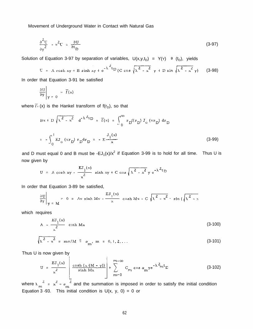
Movement of Underground Water in Contact with Natural Gas
Solution of Equation 3-97 by separation of variables, U(x,y,tD) = Y(Y) (tD), yields
In order that Equation 3-91 be satisfied
where (x) is the Hankel transform of f(rD), so that
and D must equal 0 and B must be -EJ1(x)/x2 if Equation 3-99 is to hold for all time.
now given by
(3-97)
(3-98)
(3-99)
Thus U is
In order that Equation 3-89 be satisfied,
which requires
(3-100)
(3-101)
Thus U is now given by
(3-102)
where and the summation is imposed in order to satisfy the initial condition
Equation 3 -93. This initial condition is U(x, y, 0) = 0 or
62

(3-103)
The terms cos my form an orthogonal set over the interval (0, M) so that multiplication of both
sides of Equation 3-103 by cos( my )dy and integration from 0 to M yields
The final solution for U now appears
(3-104)
Since the Hankel inversion integral is (59)
the final solution for P is
which becomes
when y is set equal to zero
where
(3-105)
P(rD,tD) = pressure drop
r D = dimensionless radius, r/rb
Jo,J1 = Bessel functions of the first kind and 0th and
63

Movement of Underground Water in Constact with Natural Gas
The pressure drop P as given by Equation 3-106 is a function of rD; i. e., radial posi-
tion at the bottom surface of the gas bubble. The question arises as what value of rD should be
employed in evaluating P, e. g. , rD = 0 (center of gas bubble) rD = 1 (edge of gas bubble) or
r D = some intermediate value between 0 and 1. This question was resolved by calculating theareal average P; i. e.
(3-107)
This areal average pressure drop is obtained by substituting P(rD,tD) from Equation
3-106 into 3-107 and performing the integration indicated in Equation 3-107.
(3-108)
The integral in Equation 3-108 cannot be evaluated analytically. For the purpose of
numerical computation, the integral was split up into parts, some independent of t D’ oneindependent of M. Thus
(3-109)
where
(3-110)
64
(3-111)
(3-112)
(3-113)

(3-115)
Each of these five integrals were evaluated on the IBM 704 computer for various M and
tD values. Their sum is equal to P and is tabulated in Appendix I as a function of M and tD.
For dimensionless time t D> 10, the integral I3 rapidly approaches a form which may
be expressed as the exponential integral
(3-117)
which in turn approaches a form yielding a time dependence of n tD, Thus the time dependence
of P approaches n tD for dimensionless time greater than 10.
It is desirable to multiply the dimensionless pressures defined by Equation 3-109 by the
factor (2M). This defines a dimensionless pressure drop Pt as a function of dimensionless time
which is analogous to that for the radial model. The dimensionless pressures corresponding to
various dimensionless times and different M values are listed in Appendix I. The dimensionless
pressures for the radial model are also presented in Appendix I for purposes of comparison.
The working equation for the thick sand model, when the Pt values from Appendix I are
used, is identical to the constant terminal rate equation for the radial model:
For dimensionless time values greater than 1000, Pt can be calculated from
(2-17)
(3-118)
where A is defined in Table 2-2.
Hemispherical Model (Constant Terminal Pressure Case)
The diffusivity equation governing spherical, unsteady-state flow of a compressible liquid
through a porous medium appears
where
(3-119)
(3-120)
65

Movement of Underground Water in Contact with Natural Gas
and y is the specific weight in pounds force per cubic foot. The independent variables r and t in
Equation 3-119 can be put into dimensionless form by defining dimensionless radius and time as
(3-121)
(3-122)
where rb is the reservoir radius. Equation 3 - 119 now becomes
(3-123)
are
In this case the initial and boundary conditions for which Equation 3-123 is to be solved
(3-124)
(3-125)
(3-126)
Definition of a new dependent variable
(3-127)
causes Equations 3-123 - 1-126 to become
(3-128)
(3-129)
(3-130)
(3-131)
Equation 3-128 can be simplified by noting that if another substitution
(3-132)
(3-133)
66

Thus Equation 3-128 is equivalent to
which is somewhat simpler to solve than is Equation 3-128.
The conditions (Equations 3- 129 - 3-131) become in terms of V
(3-135)
(3-136)
(3-137)
(3-138)
Equation 3-135, subject to conditions (Equations 3-136 -3-138), can be easily solved
by use of the Laplace transformation. Letting
(3-139)
denote the Laplace transformation of V(VD,tD),we have upon transforming Equation 3-135,
which is easily solved to yield
If Equation 3-137 is to be satisfied, c1 must be zero so that
Satisfaction of Equation 3-138 requires that
(Equation 3-143 is the Laplace transformation of Equation 3-138). Thus
and
(3-140)
(3-141)
(3-142)
(3-143)
(3-144)
(3-145)
67
Movement of Underground Water in Contact with Natural Gas
the final solution for the transform (rD, s) is therefore
(3-146)
Taking the inverse transform of Equation 3-146, we have
and employing Equation 3-132 to obtain U(rD, tD),
(3-147)
Finally, use of Equation 3-127 gives from U as
(3-148)
(3-149)
Equation 3-149 is the final solution for the potential distribution (rD, tD). The complementary
error function (erfc is simply an integral)
(3-150)
which is tabulated on page 24 of Jahnke and Emde (30).
The rate of water influx across the hemisphere r = rb is given from Darcy’s Law as
(3-151)
where the positive sign is used because influx is in the negative r direction (direction of decreas-
ing r). The area A of a hemisphere is so that we might insert for A in Equation 3-151.
However, the gas-water interface was assumed to be a hemisphere only so that the water flow
could be treated mathematically as spherical. Actually, the interface is closer to being flat so
that a more appropriate area A is Thus Equation 3-151 becomes
Differentiation of as given in Equation 3 - 149 yields
(3-152)
(3-153)
68
Insertion of Equation 3-153 into Equation 3-153 gives the water influx rate as
The cumulative amount of water influx (volume) is given by integration of ew,
(3-154)
(3-155)
(3-156)
(3-157)
Elliptical Model (Pressure Case)
The diffusivity equation governing unsteady-state liquid flow through a porous medium
has been derived in the literature and is given here as Equation 3-158
(3-158)
where p = liquid pressure, psia
C = sum of liquid and porous medium compressibilities, vol/vol-psia
= porous medium mobility, ft2/sec-psia
= porous medium porosity, fraction
The form of the term is determined by the geometry of the particular flow model being
considered. For example if the flow model is a circular cylinder and if the flow is assumed radial,
then Equation 3-158 becomes
(3-159)
where r is the radius from the center of the cylindrical flow model.
The form of the diffusivity equation governing unsteady-state liquid flow in a porous
medium having elliptic boundaries is obtained by expressing in elliptic coordinates. Thegeneral expression for the three-dimensional Laplacian of a dependent variable p(u, v, w) in
curvilinear coordinates u, v, and w is
69
Movement of Underground Water in Contact with Natural Gas
(3-160)
where
(3-161)
(3-162)
(3-163)
The following relations between elliptic and Cartesian coordinates can be used to determine α , β ,
ξ from Equations 3-161, 3-162, and 3-163
x = cosh (u) cos (v) (3-164)
y = sinh (u) sin (v) (3-165)
z = w (3-165)
= focal length of ellipse
Substitution of α , β and ξ into Equations 3-160 and 3-158 then yields
(3-166)
Equation 3-166 is the diffusivity equation relating the dependent variable p to the elliptic planar
coordinates u and v and the time variable t.
The geometric relationships between the Cartesian planar coordinates x and y and the
elliptic planar coordinates u and v are shown in Figure 2-9. The confocal ellipses (along which
u is constant) and the confocal hyperbolas (along which v is constant) are mutually orthogonal or
perpendicular to one another at points of intersection just as the lines x = constant and y = con-
stant are mutually orthogonal in the Cartesian coordinate system.
Darcy’s flow equation relates the superficial fluid velocity in a porous medium to the pres-
sure gradient in the manner
(3-167)
where V is the velocity vector, feet per second, y is the liquid specific weight, pounds force per
cubic foot and w is the vertical distance coordinate, feet. The gradient of the dependent variable
p(u, v, w) is expressed in the elliptic coordinates u, v, and w as
70
(3-168)

Substitution of the previously determined expressions for α , β and ξ yields
Substituting from Equation 3-169 into Equation 3-167, one obtains
(3-169)
(3-170)
At any given point on a ellipse, u = constant, the term is proportional to the
velocity vector component in the v direction, or in the direction tangent to the ellipse at that
point. The term can therefore be deleted from Equation 3-170 in this case, since the
flow across elliptic boundary u = constant is being considered. Also the term
in Equation 3-170 can be set equal to zero since Making these simplifications inEquation 3-170, one obtains
(3-171)
where K = a constant and
V = V(v, t) = fluid velocity in negative u direction across the elliptic boundary u = K,
feet per second.
The volumetric rate of liquid flow across an infinitesimal area element, dA, at the
elliptic boundary is simply VdA, or
(3-172)
where dA = hds, square feet
S = arc length on ellipse u = K, feet
q = q(t) = volumetric liquid flow rate across entire elliptic boundary, u = K, cubic
feet per second
The differential arc length ds is given on the ellipse by
(3-173)and substitution of
for dA in Equation 3-172 yields
71

(3-174)
Because of flow symmetry about the x and y axes (see Figure 2-9), q can be obtained by integrating
Movement of Underground Water in Contact with Natural Gas
dq over the first quadrant from v = 0 to v = /2 and multiplying the result by four.
A dimensionless water influx term Qt can now be defined as
(3-175)
(3-176)
where dimensionless time for elliptic flow and
The actual cubic feet of cumulative water flow across the elliptic boundary up to time t is related
to Qt as
(3-177)
The values of Qt as a function of dimensionless time, tD, given by Equation 3-176 was determined
by solving Equation 3-166 by numerical methods. This work is described by Coats, Tek and Katz
(7).
72
CHAPTER 4
DATA REQUIRED FOR FIELD CALCULATIONS
To make reservoir calculations, it is necessary to have information on the properties of
the fluids and the character of the porous beds. The pressure at the gas-water contact is required
for water movement calculations. The usual procedure in obtaining this pressure is to use gas
well pressures as the basic data. Generally the gas bubble is assumed to be at a weighted average
pressure considered uniform throughout the gas phase. The production-pressure history of a gas
field provides the first approximation of the gas pore volume. This initial gas pore volume may
be used along with gas production or injection data to calculate changes in pressure which would
be caused solely by the production or injection of gas if the pore volume were constant.
Fluid Properties
The density of natural gas is used to convert metered quantities of gas to volumes in the
reservoir. Calculation of bottom hole pressures from well head pressures also employs gas
densities. The customary method of expressing the density of the gas is the gas law involving the
compressibility factor: (35 )( 48)
pV = (4-1)
where p = pressure, psia
V = volume of n moles of gas at pressure, p, and temperature, T, cubic feet
Z = compressibility factor, dimensionless
n = pound moles of gas
R = gas constant =
T = temperature, oR = OF + 460
In case it is desired to use an expression for the volume of gas, then V in cubic feetper pound at T and p becomes
(4-2)
where G = gas gravity = molecular weight/29. At 14.7 pounds per square inch absolute and
60°F, one pound mole of an ideal gas has a volume of 379 cubic feet. The compressibility factor
is often expressed as a function of temperature, pressure and gas gravity in chart form. Figure
4-1 is the compressibility factor for natural gas of 0.6 gravity, containing no more than minor
concentrations of carbon dioxide, nitrogen, or other non-hydrocarbons. The American Gas
Association report on gas measurement (48)(35) provides tables of supercompressibility factors,
FPV, which are equal to The Handbook of Natural Gas Engineering (35) provides tables of
compressibility factors as a function of gas gravity, reduced pressure and reduced temperature.
Since field calculations may employ computers, it is convenient to have the compressibility
73
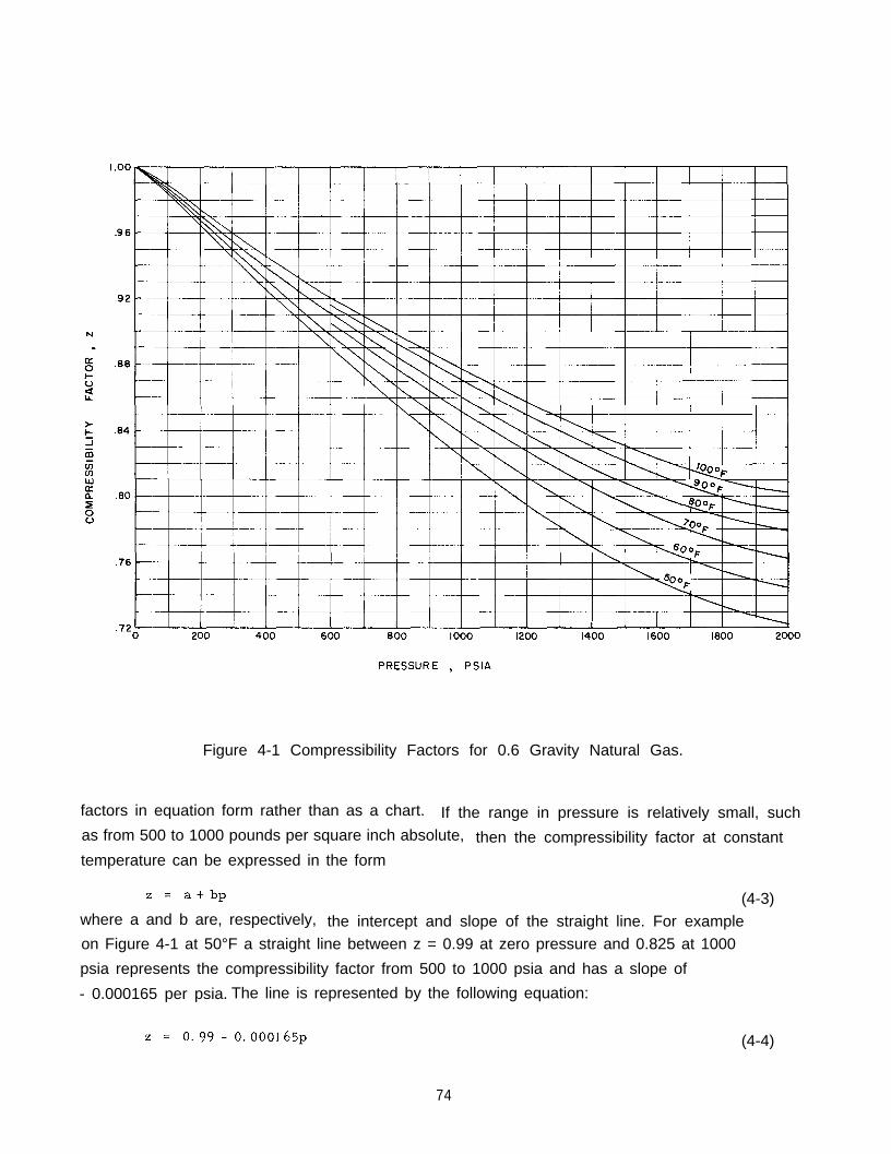
Figure 4-1 Compressibility Factors for 0.6 Gravity Natural Gas.
factors in equation form rather than as a chart. If the range in pressure is relatively small, suchas from 500 to 1000 pounds per square inch absolute, then the compressibility factor at constanttemperature can be expressed in the form
(4-3)where a and b are, respectively, the intercept and slope of the straight line. For exampleon Figure 4-1 at 50°F a straight line between z = 0.99 at zero pressure and 0.825 at 1000
psia represents the compressibility factor from 500 to 1000 psia and has a slope of
- 0.000165 per psia. The line is represented by the following equation:
(4-4)
74

Table 4-1 Values of the Coefficient, Amn Used in Equation for Compressibility Factors.
(Sarem)(56)( Courtesy Oil and Gas Journal)
Table 4-2 Legendre Polynomials of Degree 0-5. (Sarem)( 56)( Courtesy Oil and Gas Journal)
For certain ranges of pressure, z is not well represented by a straight line function of
pressure. It may be desirable to include the effect of temperature when expressing values of z.
A table of z values as a function of temperature and pressure can be used with computers with
sufficient storage. Sarem (56) developed a method for computing z factors requiring 36 coefffic-
ients which is well suited to small and medium-sized computers where the computer memory
storage limitation may be a serious factor.
where
(4-5)
(4-6)
(4-7)
Values of Amn, Pmn and Pmn are presented in Tables 4-1 and 4-2. The basis for the equation isthe compressibility chart by Brown and Katz (32)(35).
The compressibility of water is given by Figure 1-6. The density of pure water is notused as such in unsteady state water movement calculations.. At 60°F and one atmosphere, the
density is 62.4 pounds per cubic foot.
The viscosity of pure water is given on Figure 4-2. Figure 4-3 presents the effect ofsodium chloride concentration on the viscosity of water at atmospheric pressure (29). The viscosity
75

Figure 4-2 Viscosity of Water.
of gases, not normally required in water movement calculations, are given for gases of variousspecific gravities on page 176 of reference (35).
Reservoir Properties
The dimensions and character of reservoir rock vary from field to field and normally
are measured for each case. The porosity and permeability are obtained by routine analyses on
cores. In addition to permeability data on cores, well tests may be used to obtain insitu permea-
bilities. The method for calculating the permeability from pump tests on an aquifer is illustrated
in Chapter 7. For methods of determining rock permeability from gas well flow in steady state or
from pressure draw-down or pressure build-up data, the reader is referred to page 443 of refer-ence (35). Permeabilities calculated from such well tests are normally more representative
of the formation than these from cores.
Rock compressibility has been measured by finding the combined compressibility of
water and rock in the laboratory (14)(17). By calculating the effect of water compressibility on
76
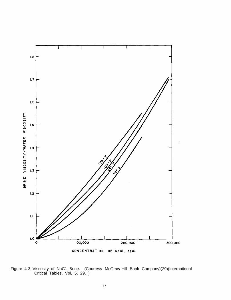
Figure 4-3 Viscosity of NaC1 Brine. (Courtesy McGraw-Hill Book Company)(29)(InternationalCritical Tables, Vol. 5, 29. )
77
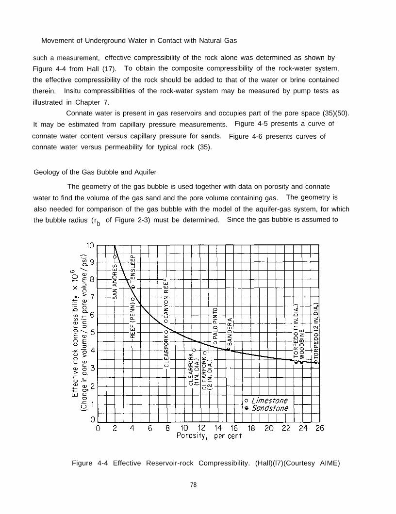
Movement of Underground Water in Contact with Natural Gas
such a measurement, effective compressibility of the rock alone was determined as shown by
Figure 4-4 from Hall (17). To obtain the composite compressibility of the rock-water system,
the effective compressibility of the rock should be added to that of the water or brine contained
therein. Insitu compressibilities of the rock-water system may be measured by pump tests as
illustrated in Chapter 7.
Connate water is present in gas reservoirs and occupies part of the pore space (35)(50).
It may be estimated from capillary pressure measurements. Figure 4-5 presents a curve of
connate water content versus capillary pressure for sands. Figure 4-6 presents curves of
connate water versus permeability for typical rock (35).
Geology of the Gas Bubble and Aquifer
The geometry of the gas bubble is used together with data on porosity and connate
water to find the volume of the gas sand and the pore volume containing gas. The geometry is
also needed for comparison of the gas bubble with the model of the aquifer-gas system, for which
the bubble radius (rb of Figure 2-3) must be determined. Since the gas bubble is assumed to
Figure 4-4 Effective Reservoir-rock Compressibility. (Hall)(l7)(Courtesy AIME)
78
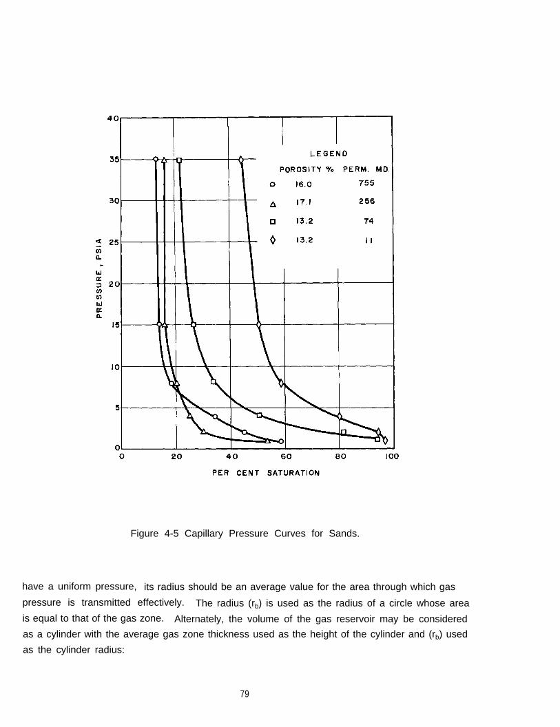
Figure 4-5 Capillary Pressure Curves for Sands.
have a uniform pressure, its radius should be an average value for the area through which gas
pressure is transmitted effectively. The radius (rb) is used as the radius of a circle whose area
is equal to that of the gas zone. Alternately, the volume of the gas reservoir may be considered
as a cylinder with the average gas zone thickness used as the height of the cylinder and (rb) used
as the cylinder radius:
79
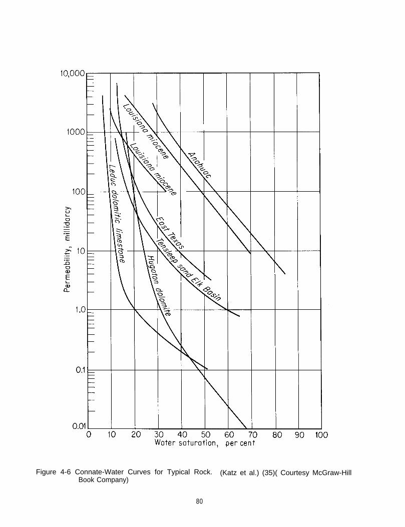
Figure 4-6 Connate-Water Curves for Typical Rock. (Katz et al.) (35)( Courtesy McGraw-HillBook Company)
80

(4-8)
wherer b = radius of bubble, feet
Vr = gas reservoir volume, cubic feet
Vj = net gas pore volume in the reservoir, cubic feet
h = average gas zone thickness, feet
g = fractional porosity containing gas
The thickness of the aquifer is needed for determination of the dimensions of the model- - -representing the gas-water system. This information is accumulated from core data and logs for
wells drilled in the area. Geologists and petroleum engineers are familiar with the preparation
of isopachous maps. Abundant data are normally available on the gas reservoir thickness. It
should be emphasized that not only is the fomation thickness at the gas reservoir of interest, but
also the surrounding aquifer at distances of ten miles or more from the gas bubble.
As will be explained in Chapter 5, for reservoirs which have operating gas-injection or
withdrawal-pressure data, the geometry and reservoir characteristics are required only for the first
approximation of water movement.
Reservoir Temperature
The reservoir temperature is usually measured by a recording or maximum thermometer.
Ground temperature at 100 feet from the surface is approximately equal to the mean average annual
atmospheric temperature, and hence varies with the locality. Many temperature-depth relation-
ships are represented by straight lines starting at the 100 foot value. A temperature-depth line
should be determined for each storage project.
Gas Reservoir Pressure
The pressure at the interface between the gas bubble and the aquifer is normally taken
as the average gas bubble pressure. Likewise, the volume occupied in the reservoir by a given
quantity of gas is computed from the reservoir temperature and an average reservoir pressure.
For high permeability reservoirs, the gas bubble pressure may be uniform within +0.5 per cent
and there is little problem in arriving at an average reservoir pressure. For low-permeability
reservoirs or those with a high permeability in the center and low permeability on the edges,
much effort is required to compute an acceptable average gas bubble pressure.
Calculation of Reservoir Pressure from Well Head Pressure
Gas field pressures are often reported from measurements at the well head. A calcu-
lation may be made to obtain the bottom hole or reservoir pressure from the well head pressure
data. The relationship between the bottom hole pressure and the well head pressure is given by
81
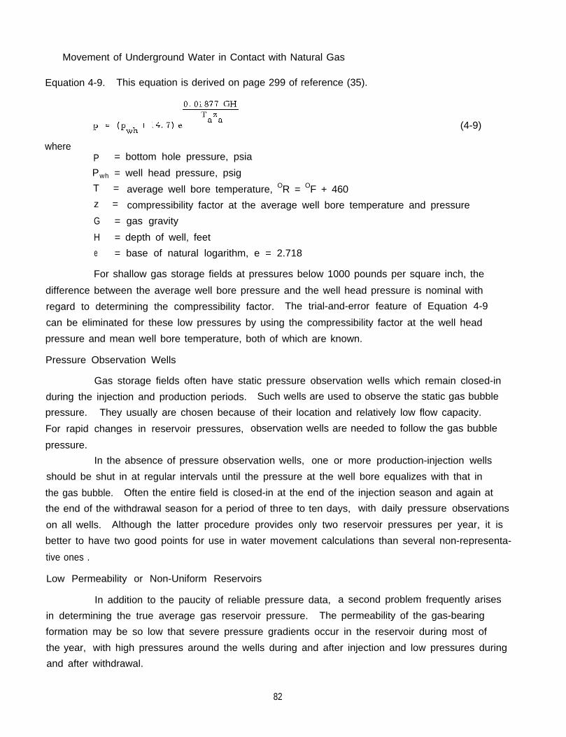
Movement of Underground Water in Contact with Natural Gas
Equation 4-9. This equation is derived on page 299 of reference (35).
(4-9)
whereP = bottom hole pressure, psia
Pwh = well head pressure, psigT = average well bore temperature, OR = OF + 460z = compressibility factor at the average well bore temperature and pressure
G = gas gravity
H = depth of well, feet
e = base of natural logarithm, e = 2.718
For shallow gas storage fields at pressures below 1000 pounds per square inch, the
difference between the average well bore pressure and the well head pressure is nominal with
regard to determining the compressibility factor. The trial-and-error feature of Equation 4-9
can be eliminated for these low pressures by using the compressibility factor at the well head
pressure and mean well bore temperature, both of which are known.
Pressure Observation Wells
Gas storage fields often have static pressure observation wells which remain closed-in
during the injection and production periods. Such wells are used to observe the static gas bubble
pressure. They usually are chosen because of their location and relatively low flow capacity.
For rapid changes in reservoir pressures, observation wells are needed to follow the gas bubble
pressure.
In the absence of pressure observation wells, one or more production-injection wells
should be shut in at regular intervals until the pressure at the well bore equalizes with that in
the gas bubble. Often the entire field is closed-in at the end of the injection season and again at
the end of the withdrawal season for a period of three to ten days, with daily pressure observations
on all wells. Although the latter procedure provides only two reservoir pressures per year, it is
better to have two good points for use in water movement calculations than several non-representa-
tive ones .
Low Permeability or Non-Uniform Reservoirs
In addition to the paucity of reliable pressure data, a second problem frequently arises
in determining the true average gas reservoir pressure. The permeability of the gas-bearing
formation may be so low that severe pressure gradients occur in the reservoir during most of
the year, with high pressures around the wells during and after injection and low pressures during
and after withdrawal.
82

Variations in permeability often occur within the reservoir, with the center having a
high permeability and the outer areas a low permeability. Methods for predicting the pressure
behavior have been developed based on models involving high and low permeability for various
parts of the reservoir (16).
One method of obtaining the average reservoir pressure at the end of a shut-in period
is to contour the field for pressure and weight the pressures according to the sand volume or
pore space represented by each segment of the reservoir.
Fortunately, the rate of water movement is low in aquifers when their permeability
is low. In general, it follows that for those reservoirs for which there is uncertainty in the
gas bubble pressure because of low permeability, the water movement rate is relatively small
and thus less significant in predicting gas reservoir pressures for future injection-production
schedules.
Initial Gas Pore Volume
When geological data permit, the initial gas phase pore volume should be determined
from isopachous maps, porosity, and connate water. The initial pore volume may also be com-
puted from gas production and reservoir pressure data by a material balance.
Writing of the gas law Equation 4-1 at the initial time and at some later period when the
cumulative production and reservoir pressure are known gives an expression for Vo, the pore
volume of the reservoir if it remains unchanged.
(4-10)
(4-11)
Subtracting Equation 4-11 from Equation 4-10 and solving for Vo. with the assumption that
V2 = Vo and To = T2.
The decrease in moles of gas (no - n2) is calculated from gas production (G ) in terms of standardP
cubic feet measured at Tbase and Pbase.
(4-12)
In field units R = 10.73.
(4-13)
83

Movement of Underground Water in Contact with Natural Gas
Substituting Equation 4-13 into Equation 4-12
(4-14)
A simple solution to this equation is obtained by plotting the cumulative gas production G versusP
p/z and determining Vo. from the slope of the line.
(4-15)
where m = minus reciprocal slope of p/z line versus GP’
standard cubic feet per pounds per
square inch.
Figure 4-7 is a plot of cumulative gas production (Gp) versus the ratio of the reservoir
pressure to the compressibility factor (1 /z) for Field X. Physically, m in Equation 4-15, is
obtained by reading the values of two points on the straight line as follows:
For Figure 4-7, the value of m is
The value of Vo is 316 million cubic feet of space. A word of caution is given about using the
physical slope of the line without regard to scales.
The reader may question the propriety of using a p/z plot when water movement is or
may be involved. It is recognized that the initial pore volume computed in this manner is in error
when the volume of the gas bubble has decreased by water influx. However, the value so computedis valuable as a first approximation for use in calculating water movement either with a geometric
model or with the generalized performance method. If the difference between the predicted and
observed field pressure is large, a corrected initial pore volume is used until the best fit is
obtained between observed and calculated pressures. Thus the Vo taken from the p/z chart is
normally not the value used in predicting the reservoir behavior. For Field X represented on
Figure 4-7, the initial pore volume found to give the best agreement in pressure performance
was 280 million cubic feet as compared to 316 million cubic feet, showing the calculation of Vo
from the p/z chart to be in error by about 13 per cent.
84
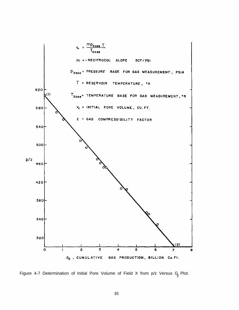
Figure 4-7 Determination of Initial Pore Volume of Field X from p/z Versus G Plot.P
85

This Page Intentionally Left Blank
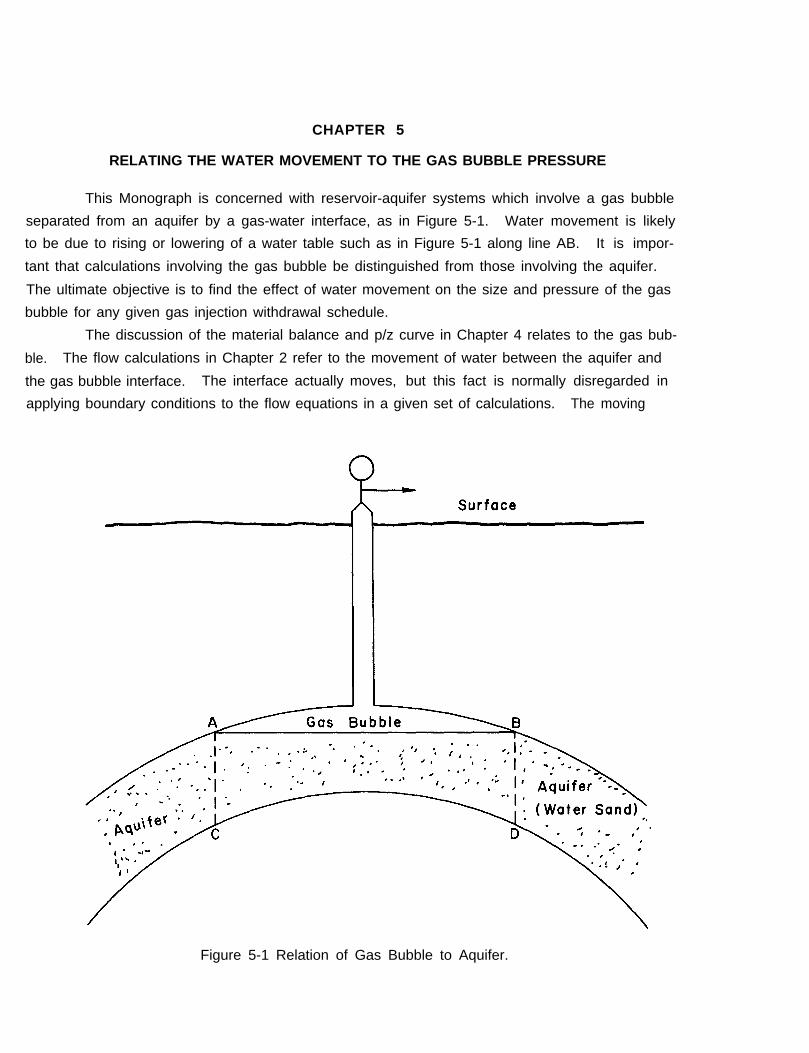
CHAPTER 5
RELATING THE WATER MOVEMENT TO THE GAS BUBBLE PRESSURE
This Monograph is concerned with reservoir-aquifer systems which involve a gas bubble
separated from an aquifer by a gas-water interface, as in Figure 5-1. Water movement is likely
to be due to rising or lowering of a water table such as in Figure 5-1 along line AB. It is impor-
tant that calculations involving the gas bubble be distinguished from those involving the aquifer.
The ultimate objective is to find the effect of water movement on the size and pressure of the gas
bubble for any given gas injection withdrawal schedule.
The discussion of the material balance and p/z curve in Chapter 4 relates to the gas bub-
ble. The flow calculations in Chapter 2 refer to the movement of water between the aquifer and
the gas bubble interface. The interface actually moves, but this fact is normally disregarded in
applying boundary conditions to the flow equations in a given set of calculations. The moving
Figure 5-1 Relation of Gas Bubble to Aquifer.

Movement of Underground Water in Contact with Natural Gas
boundary problem is treated in Chapter 8.
In practical field performance calculations, the available data are gas injection and
withdrawal quantities. However, up to this point in the Monograph, the equations presented for
water movement required data on reservoir pressure or water movement rate, neither of which
are usually available. Combination of the material balance equation for the gas bubble and thewater movement equation for the aquifer allows the use of the gas injection and withdrawal quan-
tities to predict the gas bubble pressures.The water movement equation in unsteady state was limited to either constant terminal
pressure; i. e., constant gas bubble pressures, or to constant terminal rate; i. e., constant water
movement across the gas -water interface. Since neither pressure nor water movement rates
are, in general, constant in field practice, it is necessary to resort to employing the superposi-
tion principle. Superposition Principle
The available solutions to the flow equations for water moving into and out of the gas
bubble require that the water flow rate or the gas bubble pressure be held constant. While the
pressure in a gas storage reservoir changes with time, the pressure-time curve may be approxi-
mated by a series of constant pressure steps to obtain workable solutions to the unsteady flow
equations. For each pressure step, flow calculations may be made for all desired values of time
and the composite effect is obtained by superimposing the effects of all of the increments. Thus,at the end of five time steps, the calculated cumulative water influx is the sum of five components
as shown in Figure 5-2. The first component results from the action of ∆ p1 over all five time
steps; the second results from the action of ∆ p 2over four time steps; . . . . . the fifth results from
the action of ∆ p 5 over the last time step. The constant pressure increments are chosen for as
small a time interval as possible without making the calculations too voluminous. It is clear thatbeyond a very few time steps a digital computer is required for making such calculations efficiently.
The average pressure differential for the first time step is ∆ p1 = (po- p1)/2 on Figure 5-2
For the second time step, ∆ p 2 = for the third time step ∆ p 3 and for thenth time step ∆ pn = Although the pressure in the aquifer is not uniform throughout
at the beginning of the second time step, it has been shown that this procedure gives satisfactory
results for small time steps.
With pressures in gas storage fields cycling up and down, the superposition concept
becomes further complicated by the reversals in pressure. Figure 5-3 shows how the influx and
efflux processes are combined for gas storage fields employing overpressures. The calculationsfor each pressure level must be continued until the end of the time being considered. For sometime increments water may be moving in one direction and for others in the opposite direction.
The net movement is of interest and the computer program is established to give as its solution
only the composite curve for all the increments in effect up to any given time.
A similar superposition may be made of computed pressures for increments of rates. The
88

Figure 5-2 Pressure and Cumulative Water Influx versus Time for Producing Gas Reservoir.
89

Figure 5-3 Pressure and Cumulative Water Movement versus Time for Storage Field.
90
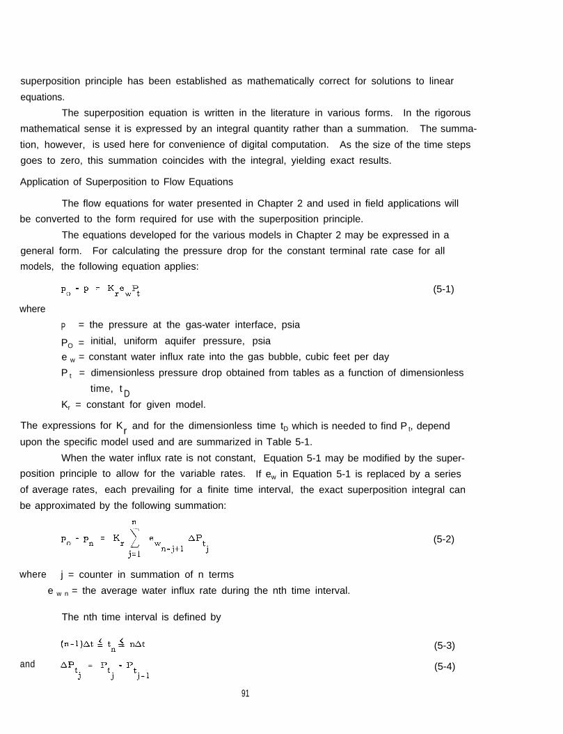
superposition principle has been established as mathematically correct for solutions to linear
equations.
The superposition equation is written in the literature in various forms. In the rigorous
mathematical sense it is expressed by an integral quantity rather than a summation. The summa-
tion, however, is used here for convenience of digital computation. As the size of the time steps
goes to zero, this summation coincides with the integral, yielding exact results.
Application of Superposition to Flow Equations
The flow equations for water presented in Chapter 2 and used in field applications will
be converted to the form required for use with the superposition principle.
The equations developed for the various models in Chapter 2 may be expressed in a
general form. For calculating the pressure drop for the constant terminal rate case for all
models, the following equation applies:
(5-1)
where
P = the pressure at the gas-water interface, psia
PO = initial, uniform aquifer pressure, psia
e w = constant water influx rate into the gas bubble, cubic feet per day
P t = dimensionless pressure drop obtained from tables as a function of dimensionless
time, t DKr = constant for given model.
The expressions for K and for the dimensionless time tDr which is needed to find P t, depend
upon the specific model used and are summarized in Table 5-1.
When the water influx rate is not constant, Equation 5-1 may be modified by the super-
position principle to allow for the variable rates. If ew in Equation 5-1 is replaced by a series
of average rates, each prevailing for a finite time interval, the exact superposition integral can
be approximated by the following summation:
where j = counter in summation of n terms
e w n = the average water influx rate during the nth time interval.
The nth time interval is defined by
(5-2)
and
91
(5-3)
(5-4)

Movement of Underground Water in Contact with Natural Gas
Table 5-1 Summary of Flow Equations for Water Movement
Constant Terminal Rate Case, p = po - KrewPt
Constant Terminal Pressure Case, We = Kp (Po - p)Qt
where the subscript j denotes time tJ:
(5-5)
Expansion of Equation 5-2 and rearrangement of terms gives an equation equivalent to Equation
5-2,
(5-6)
whe re (5-7)
92
(5-8)
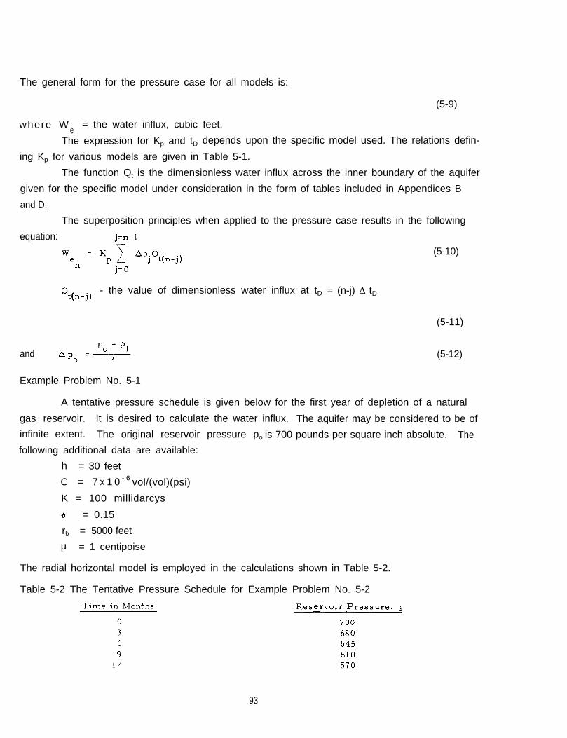
The general form for the pressure case for all models is:
(5-9)
where W = the water influx, cubic feet.eThe expression for Kp and tD depends upon the specific model used. The relations defin-
ing Kp for various models are given in Table 5-1.
The function Qt is the dimensionless water influx across the inner boundary of the aquifer
given for the specific model under consideration in the form of tables included in Appendices B
and D.
The superposition principles when applied to the pressure case results in the following
equation:
- the value of dimensionless water influx at tD = (n-j) ∆ tD
(5-10)
(5-11)
and (5-12)
Example Problem No. 5-1
A tentative pressure schedule is given below for the first year of depletion of a natural
gas reservoir. It is desired to calculate the water influx. The aquifer may be considered to be of
infinite extent. The original reservoir pressure po is 700 pounds per square inch absolute. The
following additional data are available:
h = 30 feet
C = 7 x 1 0 - 6 vol/(vol)(psi)
K = 100 millidarcys
= 0.15
rb = 5000 feet
µ = 1 centipoise
The radial horizontal model is employed in the calculations shown in Table 5-2.
Table 5-2 The Tentative Pressure Schedule for Example Problem No. 5-2
93
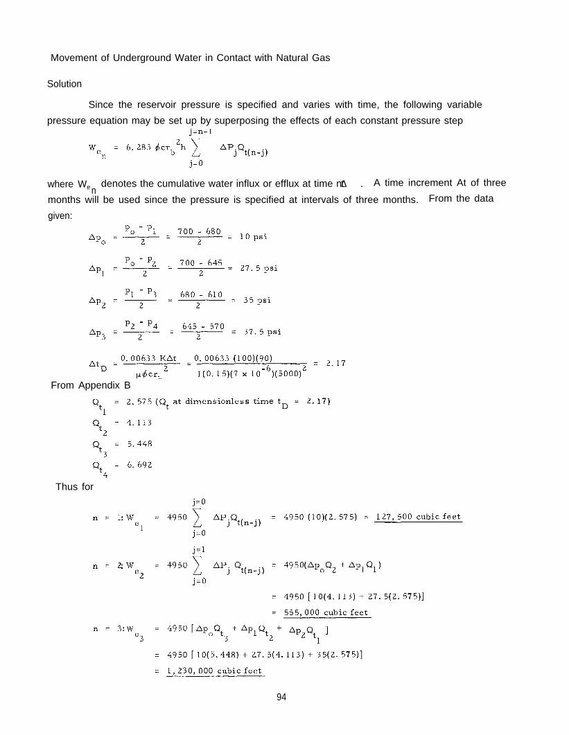
Movement of Underground Water in Contact with Natural Gas
Solution
Since the reservoir pressure is specified and varies with time, the following variable
pressure equation may be set up by superposing the effects of each constant pressure step
where We denotes the cumulative water influx or efflux at time n ∆ t . A time increment At of threen
months will be used since the pressure is specified at intervals of three months. From the data
given:
From Appendix B
Thus for
94

If the aquifer in the above example had been limited in extent then the Qt values would
have been taken from Appendix D.
Prediction of Gas Reservoir Performance
For field problems, the data usually available are the injection and production of gas
into the gas bubble. The desired result of the calculation is the gas reservoir pressure. To
accomplish this, the material balance equation for the gas bubble is combined with the water
movement equation. By combining the gas law, Equation 4-2, with the expression for the compressi-
bility factor, Equation 4-3, one obtains:
(5-13)
where Sj = njRT. The subscript j simply denotes that the variable is to be taken at time t = j ∆ t .
Equation 5-13 should be considered as one equation in the two unknowns Vj (reservoir pore volume
at time j ∆ t) and pj. The nj is the known or specified gas-in-place at time j ∆ t .
Solving Equation 5-13 for Sj, nj and using Gpj as the cubic feet of cumulative production
pbase and Tbase:
(5-14)
(5-14a)
The variable pressure or the variable rate equation for the model considered serves as
a second equation in the two unknowns, V. and p. of Equation 5-13.J J
The Variable Rate Case
The average water influx rate during the jth time interval is numerically equal to the
decrease in the gas bubble volume during the same period:
95

Movement of Underground Water in Contact with Natural Gas
Combining Equations 5-13 and 5-15:
By isolating the term for j = 1 from the summation in Equation 5-2 and solving for e
From Equation 5-17 and 5-16 pn may be evaluated as:
and
(5-15)
(5-16)
(5-17)
(5-18)
(5-19a)
The reservoir pressure and water influx rates can be calculated by repeated application of
Equations 5-17 and 5-18.
In the above procedure p1 is calculated first then , p2, etc... The method described
above requires that the values of Ko and Vo be determined from the best information available on
the reservoir such as geological data, core data, pumping tests, etc.
Alternately, an equivalent expression for pn can be obtained by expanding Equation 5-6 to
obtain
Substitution of nnRT for Vn in Equation 5-20 and solution for pn yields
(5-20)
**Note that although Equations 5-18 and 5-21 are identical, they have different definitions for Bnand Cn since alternate forms of the superposition principle were used. These equations willgive identical results for pn when the corresponding values for Cn and Bn are used.
96
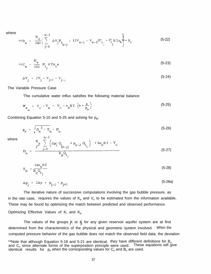
where
The Variable Pressure Case
(5-22)
‘The cumulative water influx satisfies the following material balance:
Combining Equation 5-10 and 5-25 and solving for p :n
where
(5-23)
(5-24)
(5-25)
(5-26)
(5-27)
(5-28)
(5-28a)
The iterative nature of successive computations involving the gas bubble pressure, as
in the rate case, requires the values of Kp and Vo to be estimated from the information available.
These may be found by optimizing the match between predicted and observed performance.
Optimizing Effective Values of Kr and Kp
The values of the groups K or K for any given reservoir aquifer system are at firstr Pdetermined from the characteristics of the physical and geometric system involved. When the
computed pressure behavior of the gas bubble does not match the observed field data, the deviation
**Note that although Equation 5-18 and 5-21 are identical, they have different definitions for Bnand Cn since alternate forms of the superposition principle were used. These equations will giveidentical results for pn when the corresponding values for Cn and Bn are used.
97

Movement of Underground Water in Contact with Natural Gas
may be due to misrepresentation of the physical system by the particular value of Kr or Kp used.
This in turn may be due to the value of some particular property used in the formula to compute
the group Kp or Kr. It is also entirely possible that the model is not representative due to differ-
ences in geometry or to reservoir inhomogeneities.
Rather than varying an individual variable to seek a better fit between the field data and
calculate performance, the whole group Kr or Kp may be systematically varied to optimize the
fit. Figure 5-4 shows the result of systematic variation of Kp and the dimensionless time coef-
ficient in an actual field study (6). The ordinate, per cent deviation, is a
measure of the difference between observed and calculated field behavior. It may be expressed
as the average per cent deviation between calculated and observed pressures or between calcu-
lated and observed pore volumes. Figure 5-4 shows that the minimum deviation varies only
slightly with the time coefficient provided the optimum Kp value is used for
each value of this coefficient. At a given value of the coefficient, the deviation varies markedly
with Kp . Thus a satisfactory procedure for optimizing parameters involves calculation of
from reservoir and fluid characteristics and determination of Kp (or Kr if variable
rate equation is used) by minimizing the per cent deviation between observed and calculated
field behavior.
Figure 5-4 Optimization of Kp. (Coats)(6)
98

Optimizing Initial Gas Pore Volume, Vo
The initial gas pore volume, Vowhich may be computed on an assumption of no water
movement, is likely to be in error. It is possible to obtain a more accurate value of Vo by a
sequence of trial and error calculations. This sequence of calculations seeks to determine the
Vo which results in the minimum deviation between observed and calculated pressures. An
example of this trial and error procedure is given in Chapter 9. Briefly, it consists of repeating
the full calculation for optimizing Kr or Kp with several assumedvalues of Vo The deviation
between the calculated and observed pressures is plotted versus Vo to find that Vo which corres-
ponds to the minimum deviation.
The match between calculated and observed pressures is dependent upon two physical
phenomena. They are the gas injection or production and the unsteady state water movement into
or out of the aquifer. When a gas reservoir, subject to water drive, is produced continuously at
substantially a constant rate, this optimization procedure has been found to be indecisive. Since
both water flux and gas injection or production influence gas bubble pressure, there appears to
be no unique solution for a single gas flow rate. For the determination of both the degree of
water influx represented by Kr and the initial pore volume Vo, two different gas rates are needed.
Apparently, the low degree of pressure decline for a given gas production can either be due to
the presence of a large quantity of gas with a small water influx rate or to a smaller gas quantity
with a higher water influx rate. If the production rate is changed for a period of time, then the
independence of the water movement and volumetric behavior will allow an optimization giving a
unique value of Vo, initial gas pore volume. Only one combination of gas bubble volume and water
movement rate will give the observed pressure behavior.
The cyclic nature of gas storage is believed to permit an unusual degree of optimization
because the water movement not only changes with time but even reverses in direction. Cycling
around a pressure other than the initial aquifer pressure aids in the optimization procedure.
99

This Page Intentionally Left Blank

CHAPTER 6
GENERALIZED METHOD FOR PERFORMANCE CALCULATION FROM FIELD DATA
A calculation procedure for predicting the performance of water drive gas reservoirs
without the usual assumptions of simplified, idealized geometry and homogeneity is presented in
this chapter. Solutions of the diffusivity equation governing the movement of water in aquifers
have been given in earlier chapters for various geometric configurations of reservoir-aquifer
systems. These solutions are all based on some simplifying assumptions which idealize the con-
sidered field model to some extent. Assumption of uniform formation properties, a gas bubble
of constant volume and fixed geometry for the system are typical of those needed for developing
analytical solutions for the flow equations. Actual characteristics of aquifers encountered in pro-
duction or storage operations, however, are often far from those described by various models.
The edge of the gas bubble is not perfectly circular, for example. In many instances this inter-
face between the gas and water may not be accurately approximated by either a linear or a radial
geometry. The presence of communcating or non-communicating faults, inhomogeneities such as
local variations of porosity and permeability, anisotropy (directional variations of properties),
the fact that the edge of the gas bubble is never at a fixed location, and other factors may prevent
the actual field problem from being accurately represented by one of the geometric models treated
earlier. Under these circumstances it becomes quite desirable to develop a characteristic function
which will adequately represent the past behavior and accurately predict the future performance of
a particular field. The purpose of this chapter is to present a method for developing such a
characteristic function for a field using production-pressure data obtained from that field. The
method is a modification of the “resistance function” concept formulated by Hutchinson and Sikora
(28). Hicks, Weber and Ledbetter (21) presented a related treatment using both analog and digital
computers.
The use of the method is limited to instances in which field data are available. It is not
useful, for example, in predicting the performance of an aquifer storage project before gas injec-
tion is initiated. In cases such as this, where no field data are available, a geometric model must
be used.
The Logic of the Resistance Function
It was shown in Chapter 5 that when the calculations for a given model and field data do
not match, the term Kr or Kp may be varied to optimize the fit. If the curve KrPt product versust is plotted for each of the geometric models,one obtains a curve which is characteristic of the
response of the gas bubble pressure to water influx or efflux across its boundaries. This responseis measured in terms of pressure drop per unit rate of water influx, pounds per square inch per
cubic foot per day. It is called the resistance function for that particular aquifer-gas reservoir
System. In the process of optimizng Kr the characteristic curve for a particular system changes
101

Movement of Underground Water in Contact with Natural Gas
whenever the value of Kr is changed. Once the value of Kr is optimized then the shape of the
characteristic curve becomes finalized.
It is theoretically possible to compute a function for any irregular and heterogeneous
system which corresponds to the KrPt product in regular homogeneous systems of known geometry.
Such a function, employed in place of the KrPt product in the geometric model equations, would
then characterize the system behavior. The methods presented in this chapter demonstrate means
of calculating the equivalent KrPt function from field performance data. This function Z is called
the resistance function. For many aquifer-gas reservoir systems, both Kr and Pt are initially
unknown. Since, however, it is the product of these quantities which is actually used in the system
performance calculations, it is not necessary to differentiate between them if their product may
be determined. Determination of the resistance function, Z, for a system from field data corres-
ponds to determining the KrPt product as a function of time.
Every geometric model exhibits a Pt curve which becomes linear or otherwise smooth at
large times, Figure 2-13. The KrPt curve is, therefore, also a smooth and regular function at
large time, such that it may be extrapolated with ease. Since the resistance function, Z, corres-
ponds to the KrPt product for the system, analogy indicates that it may be extrapolated for use in
future calculations.
Development of the Concept
When the partial differential equation describing the movement of water in aquifers is
solved for radial, linear, cylindrical, spherical or elliptical coordinate systems for the constant
terminal rate boundary conditions, the solution may be written in the following form for all the
geometries:
(6-1)
where
Po = the initial or equilibrium pressure in aquifer
Pt = the pressure at time t at the edge of the gas bubble. This pressure is also assumed
to prevail approximately throughout the gas bubble as observed in many fields.
Kr = group of reservoir and fluid properties determined for the particular model. The
values of Kr for various models are given in Table 5-1.
e w = constant water influx rate into the gas bubble
P t = the dimensionless pressure, evaluated at aquifer gas bubble boundary, a tabulated
function of dimensionless time for the particular geometric model considered.
Figure 2-13 illustrates the various forms of Pt vs tD curves for some of the different geometries
considered in Chapter 2.
If Equation 6-1 is rearranged so that it appears as
(6-2)
102
Then it is seen that for a constant water influx rate, ew the pressure drop below the equilibrium
value per unit rate of water influx at the gas-water interface at any time, t, is given by the pro-
duct of Kr and the function Pt. The KrPt vs time curve has a certain fixed shape for each geometric
model when the parameters which determine K and dimensionless time are specified. If a fieldr
has such irregular geometry and characteristics that it cannot be described by a simple geometric
model, the KrPt function could in principle be determined experimentally as follows. If at time,
to, the pressure is lowered in the gas bubble of a given field such that water starts to flow inward
past the gas-water interface at a rate, ew, and if the gas bubble pressure is continuously adjusted
so that the influx rate is maintained constant at all times, then a plot of (po- pt)/ ew versus t - towould give a particular curve which is equivalent to the KrPt versus time function for the field.
All the peculiarities of the field would be reflected in this curve. It is called the resistance func-
tion for the field. The term “resistance” arises from the terms on the left hand side of Equation
6-2. The potential drop per unit flux is analogous to electrical resistance.
An example of a resistance function is given in Figure 6-1. This figure shows the simi-
larity of the form of the dimensionless pressure function and the resistance function.
Calculation of Resistance Function from Field Data
In actual field operations the water influx rates are not generally constant. Under such
circumstances eW may be looked upon as a succession of average rates during finite periods of
time. The use of the superposition principle shown in Chapter 5 then permits a more general
equation giving the gas bubble pressure:
where ew is the average water influx rate during the nth time interval defined by:
and
Subscript j denotes the time:
(6-3)
(6-4)
(6-5)
(6-b)
Equation 6-3 follows directly from consideration of the superposition principle discussed
in the previous chapter. An analogous equation for the resistance function method may be obtained
by substituting the resistance function ∆ Zj for the product (Kr ∆ Pt ) used in summations with
the geometric models:
103

Figure 6-1 Parallel Between Resistance Function and Dimensionless Pressure Drop for aGeometric Model.
104

(6-7)
By combining Equation 6-7 with a material balance one may obtain a relationship giving AZ ndirectly in terms of the data available from the field. Computing ∆ Z1, ∆ Z2, ∆ Z3, etc. consecu-
tively, one could theoretically generate the whole resistance function curve which can be used to
predict the pressure performance of the field for any projected gas-in-place schedule.
Such a procedure is unfortunately over-sensitive to errors in pressure data. The errors
tend to be magnified because of computational instability to the point of making this method imprac-
tical and inaccurate for field calculations. In order to overcome this difficulty and render the
method less sensitive to data errors, self-correcting features for Z’s have been developed and
incorporated in the computational procedure. The modified procedure also includes an evaluation
of the apparent trends in the resistance function that are based upon comparisons with the expected
behavior of known geometric models. In the calculation of early time steps, errors in field data
generally make it impossible to compute a valid resistance function. Calculations using actual
field data have shown that much better results are obtained if the initial portion of the resistance
function curve is approximated by one of geometric models presented in Chapter 2. Figure 6-2
illustrates the time ranges for which the resistance function is first approximated by a model,
next fit directly from field data, and finally extrapolated for use in performance predictions.
The Z function from the beginning to mth time step is generated by assuming the field
to behave as a radial, thick sand, or another fixed geometry model based upon optimized values
of Kr. From time steps (m+1) to (i), the field behavior is used to generate the Z curve by indi-
vidually and sequentially computing the ∆ Zn values. During this phase of calculation each of the
current values of the Z functions are tested and corrected to minimize instabilities induced by
errors in the data. Once the corrected Z values are computed up to ith time step, then the Z
curve may be extrapolated to larger times for use in predicting performance with any postulated
gas-in-place schedule.
Steps for Calculating the Field Performance
To use the resistance function gas bubble pressures corresponding to gas injection or
withdrawal quantities, at least 15 to 30 monthly time periods are needed. The three major steps
in using the resistance function technique are the approximation with models at early times, the
fit with field data, and the extrapolation to future times, as shown on Figure 6-2. These stageswill be considered in the order in which they are used.
Given: Geological data for a gas-aquifer system and the pressure-injection or withdrawal
quantities at corresponding times. Should the production-injection data be available at odd times,
it is necessary to prepare a table of pressures(p) and corresponding cumulative gas withdrawal
quantities (Gp) at uniformly spaced times of 0, ∆ t, 2 ∆ t, 3 ∆ t , . . . . . . .
105

Figure 6-2 The Resistance Function Curve.
1. Pick a plausible model (radial, thick sand, linear, or hemispherical).
2. Estimate Vo, the original pore space. This estimate may be made from isopach maps or from
plots of p/Z versus cumulative production.
3. Calculate Kr and tD corresponding to the model using values from Table 5-1 for n = 1, 2,....... m.It is recommended to go to m = 10 if possible.
4. Calculate all the values of the variable Sn defined as nnRT for n = 1, 2,. . . . i.
106

(6-8)
where in field units:
5. From values of tD(or for linear model), obtain the values for each time step for
6. Compute (6-9)
7. Compute p1, setting n = 1 in Equation 5-18, which corresponds to the gas-water contact
pressure at the end of the first time step t1
107
(6-10)

Movement of Underground Water in Contact with Natural Gas
where(6-11)
(6-12)
8. Compute f rom
(6-13)
9. Compute pn, in indicated sequence for n = 2, 3,. . . . m from Equations 6-14 and 6-17.
where
10. Compare the calculated pressures with the observed pressures on the gas bubble,
(6-14)
(6-15)
(6-16)
(6-17)
expressed
as a sum of the absolute value of the deviations. Select a new Kr such as 2Kr and repeat cal-
culations above to obtain a new sum of the deviations. Continue selecting Kr‘s until a mini-
mum occurs in a plot of deviation versus Kr.
11. Compute ∆ Z1, ∆ Z2. . . . . ∆ Zm from:
(6-18)
12. Compute alternately ∆ Z n , pn and ew for n = (m+ 1), (m + 2). . . . . i, where i is the number of
last time increment of the remainingn available data. The equation to be used to compute AZ is:n
(6-19)
108
13. Since the initial estimate of Vo obtained from isopach maps or plot of p/z versus cumulative
production may be in error, it may be desirable to repeat steps 3 through 12 for different
values of the initial pore volume, Vo. The value of Vo which gives the best estimate of the
initial pore volume, Vo.
The pressures with asterisks denote field data while the pressures without asterisks are
computed pressures. The pressures pn are computed from:
where
and
The qua.ntities eW should be computed fromn
(6-20)
(6-21)
(6-22)
(6-23)
Self Correcting Features of the Computational Procedure
The AZ calculated at each time step is forced to comply with the following restrictions
of inequalities:
(6-24)
The inequalities 6-24 imply that whenever AZn calculated from Equation 6-19 is less
than the left hand side of the above inequality it is set equal to that left hand side value. Likewise,
if it should exceed the right hand side then it is set equal to the upper bound value represented by
the right hand side.
The factor (1 - ) is included to relax an otherwise too severe restriction. An = 0.02
has been found to work satisfactorily on the problems solved.
In order to preserve the analogy between the resistance function and the corresponding
dimensionless pressure drop curve derived from the solution of the diffusivity equation, the
“resistance function” Z must not violate three conditions as pointed out by Hutchinson and Sikora (28).
These are:(6-25)
(6-26)
109

Movement of Underground Water in Contact with Natural Gas
(6-27)
The possibility of an upward-curving resistance function is not eliminated by the restric-
tion imposed by Equation 6-24. In the process of generating the resistance function if d2Z/dt2
appears to come out positive a straight line is drawn (actually computed automatically by a digital
computer) from the last point generated such that it is tangent to the previously established portion
of the Z curve at some earlier time step as shown in Figure 6-3. This procedure smooths the
resistance function curve over several time steps whereas Equation 6-24 limits it pointwise.
Extrapolation of the Resistance Function Curve
Whenever a finite aquifer is indicated (as has been the case for several fields studied),
the plot of Zn versus n approaches a straight line as n approaches i. The extrapolation is obtained
by setting ∆ Zn for n> i as equal to ∆ Z i .
Otherwise the aquifer appears to be infinite and the equation for extrapolating the Z curve
is given as:
Figure 6-3 Illustration of “Back Correction” of the Resistance Function Curve.
110

Whenever a linear aquifer geometry is indicated, the extrapolation is performed by:
(6-29)
Given a postulated gas production schedule for times beyond i in the above problem, the
values for G may be computed corresponding to times from i to the final time o. Also theP
extrapolated Z versus time curve is now available. The values of Sn from n = i +1 to n = o may
be computed from the Gp schedule postulated, Equation 6-8.
Calculate ∆ Zn for n = i +1 to n = o by Calculate the water influx ewnfrom Equation 6-23. Pressures, pn, can now be calculated from Equations 6-20, 6-21, and 6-22.
Table 6-1 illustrates the three time periods under consideration in this process of develop-
ing and using the resistance function.
In case gas injection occurs instead of gas production, the values of Gp are negative and
e W will be negative values indicating efflux from the gas bubble.
An example calculation using the resistance function method is given in Chapter 9. Details
of a computer program to facilitate computation are given in Appendix L.
Table 6-1 Procedure for Calculation by Resistance Function
111

This Page Intentionally Left Blank

CHAPTER 7
DEVELOPMENT OF AQUIFER STORAGE FIELDS
Much of the engineering development of projects storing gas in water sands involves cal-
culation of the movement of water in contact with natural gas. The evaluation of a potential storage
structure involves water movement calculations based on a geometric model. Pump tests may be
made prior to gas injection to evaluate the cap rock and determine insitu permeability and compressi-
bility. A method is presented for locating the bubble edge at times after the storage reservoir has
been developed.
Insitu Permeability and Compressibility from Pump Tests
Laboratory tests on cores are normally made to determine the matrix permeability of
aquifer zones. However, the formation may have a different effective value than that obtained by
averaging core data. Fractures not included in test cores will influence the insitu permeability
as will other non-uniformities. Pumping tests on a well may be used to obtain the insitu permea-
bility. Coincident with this pumping, pressure observations on an adjacent well completed in the
aquifer will provide data for computation of the insitu composite compressibility of the water-sand
system. Figure 7-1 illustrates the location of wells which may be used in a pump test.
Figure 7-1 Pumping of Water Wells to Obtain Insitu Permeability and Compressibility as Well asas Cap Rock Leakage
113

Movement of Underground Water in Contact with Natural Gas
In any pump test the preferred method is to pump at a constant rate. When only a single
well is available, the water level in the pumping well is needed to obtain the insitu permeability.
When there is an observation well in addition to the pumping well, both K and c can be obtained
without knowing the water level in the pumping well. Table 7-1 lists some of the combinations
of data which can be used. The table gives information required to compute K and c from various
combinations of data.
Case 1. Pump Test on Single Well. (No measurement on well B, Figure 7-1). Drawdown and
Build-up Pressures Observed on Pumping Well Only.
The insitu permeability and compressibility of an aquifer can be calculated from the
drawdown test on a well pumping at a constant rate. The “point source” solution given by Horner (22)
in field units is
(7-1)
where po = initial aquifer pressure, psia -
rw = well radius, feet
t = time, days
P = pressure at the well bore at time t, psia
= formation porosity, fraction
K = permeability, millidarcys
µ = fluid viscosity, centipoise
Table 7-1 Variety of Tests for Insitu Permeability and Compressibility
114
C = fluid compressibility, vol/(vol)(psi)
q = water pumping rate, bbl/day
The exponential integral function (Ei) is defined as:
It may be represented (46) by the series:
If the value of x is small: i. e. , less than 0.01, then Ei( -x) can be approximated by:
Substitution of Equation 7-3in Equation 7-1 yields
or
(3-117)
(7-2)
(7-3)
(7-4)
(7-5)
(7-6)
If the well is pumped at a constant rate, then a plot of p versus log t will approach a
straight line. The slope of this line, pounds per square inch per cycle, is equal to -
If q, µ, and h are known, the insitu permeability can be calculated from the slope. While it may
appear that insitu compressibility, c, may also be calculated from these equations, the calculation
is so sensitive to errors in measurement of the radius of the well bore, rw,as to be impractical.
Unfortunately, skin effect at the well can give an erroneous slope on the drawdown curve
at early time. Therefore, the pressure build-up curve is usually used to obtain a more accurate
value for the permeability. If the total pumping time is designated by to and the shut-in time by
At, the well pressure after shut-in is given by superimposing two solutions of the form of Equation
7-6:
(7-7)
(7-8)

Movement of Underground Water in Contact with Natural Gas
A plot of pressure versus loglo will approach a straight line after the afterflow and
skin effects of the well damp out. The insitu permeability can be calculated from this slope
expressed in pounds per square inch per cycle. The slope is equal to -
Case 2. Pump Test on a Single Well, Drawdown and Build-up Pressures Observed at an Observa-
tion Well Only
The insitu permeability and compressibility of an aquifer can be calculated from the draw-
down and build-up pressures at an observation well. In Equation 7-6 rw is replaced by r, the
distance between the pumping well and the observation well. The pressure of the observation
well is given by:
(7-9)
where p, is the initial pressure of the observation well. There is no change in the equation des-
cribing the pressure build-up, Equation 7-8. The formation insitu permeability can be calculated
from the same procedure as outlined in Case 1.
An effective compressibility value may be determined by using Equation 7-9. If the
observation well pressure is plotted as (p - p,) versus loglo t, then the slope of the straight line
portion of this curve is - 162. 6 qp /Kh and the intercept of this straight line (value of p at
log1 0 t = 0 or t = 1) is:
(7-10)
from which c may be calculated. Alternatively, any point (Ap, log t) on the straight line portion
of the curve may be used in the equation:
(7-11)
to calculate c.
Case 3. Pump Test on Single Well, Drawdown and Build-up Pressures Observed at the Pumping
Well and One Observation Well
The quasi-steady state formula can be used at sufficiently large times. The pseudo-steady
state is reached when the rate of pressure decline, dp/dt, is constant and the same at both wells.
Darcy’s law can be used.
(7-12)
where q is water flow rate into the producing well. Rearranging Equation 7 - 12 and integrating
between two wells
116

or
and hence
Equation 7-15 expressed in field units is:
(7-13)
(7-14)
(7-15)
which can be used to calculate the insitu permeability. The distance rw is the radius of the pump-
ing well and r is the distance between the pumping well and the observation well.
Example Problem 7-1
An aquifer is being considered for gas storage. The sand occurs at a depth of 1250 feet
and is considered a suitable structure. The average physical properties of the sand determined
from core data are porosity 14.5 per cent, permeability 168 millidarcies, and sand thickness
164 feet.
A well in the aquifer was pumped at 1370 barrels per day and the pressure observed at
both the pumping well and a neighboring well, 500 feet away, during pressure drawdown and build-
up* Predict the insitu permeability of the sand and the effective compressibility of the aquifer.The pressure build-up data for the pumpingwell are given in Table 7-2 and pressure drawdown data
for the observation well are given in Table 7-3.
Solution to Example 7-1
A. Determination of the insitu permeability using the pressure build-up data on the
pumping well. In Equation 7-8
substitute ∆ p = p - po to obtain
(7-8)
From the build-up data, determine (to + ∆ t) ∆ t and ∆ p for each data point
(7-17)
117

Movement of Underground Water in Contact with Natural Gas
Table 7-2 Pressure Build-up Data - Pumping Well
Table 7-3 Pressure Drawdown - Observation Well
A plot of ∆ p versus n is shown in Figure 7-2. The slope is -3.55 pounds per
square inch per cycle. Hence
*The difference in distance to the initial water level is due to a difference in the height of thewellheads above sea level.
118
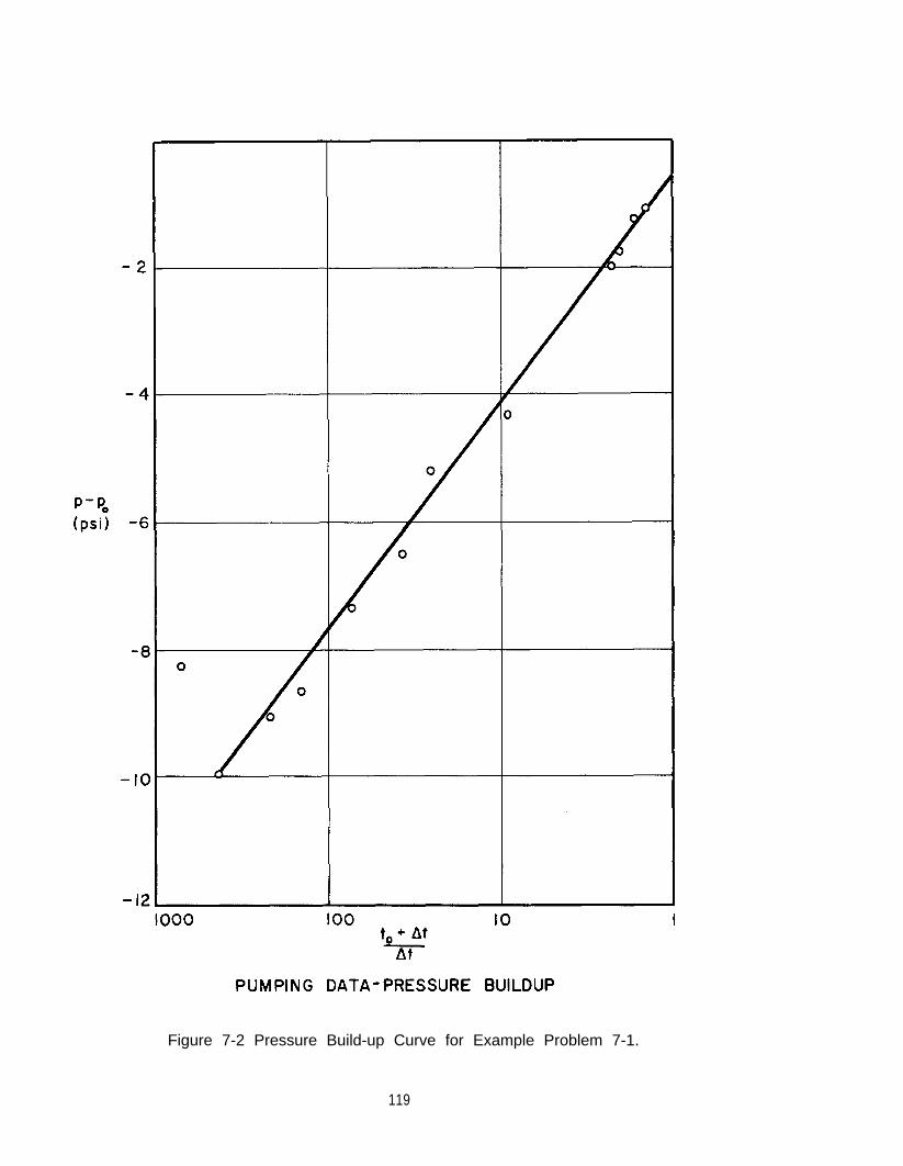
Figure 7-2 Pressure Build-up Curve for Example Problem 7-1.
119
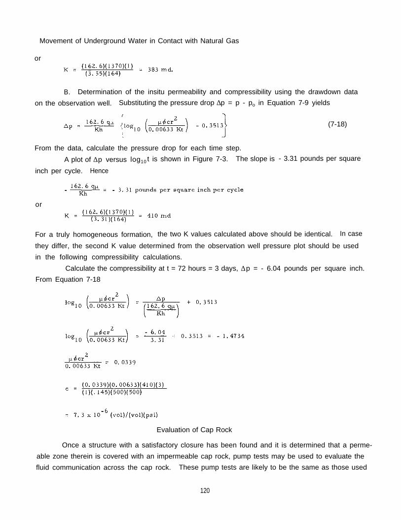
Movement of Underground Water in Contact with Natural Gas
or
B. Determination of the insitu permeability and compressibility using the drawdown data
on the observation well. Substituting the pressure drop ∆ p = p - po in Equation 7-9 yields
(7-18)
From the data, calculate the pressure drop for each time step.
A plot of ∆ p versus log10 t is shown in Figure 7-3. The slope is - 3.31 pounds per square
inch per cycle. Hence
or
For a truly homogeneous formation, the two K values calculated above should be identical. In case
they differ, the second K value determined from the observation well pressure plot should be used
in the following compressibility calculations.
Calculate the compressibility at t = 72 hours = 3 days, ∆ p = - 6.04 pounds per square inch.
From Equation 7-18
Evaluation of Cap Rock
Once a structure with a satisfactory closure has been found and it is determined that a perme-
able zone therein is covered with an impermeable cap rock, pump tests may be used to evaluate the
fluid communication across the cap rock. These pump tests are likely to be the same as those used
120
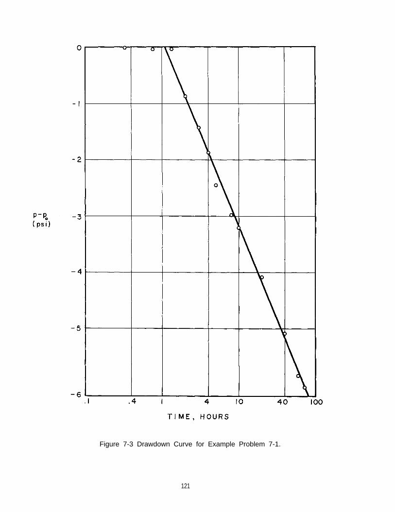
Figure 7-3 Drawdown Curve for Example Problem 7-1.
121

Movement of Underground Water in Contact with Natural Gas
to provide data for determining the insitu permeability of the prospective storage formation and
its insitu compressibility.
Figure 7-1 shows the completion of three wells in a prospective aquifer project. Twoare completed in the prospective storage formation and one in the first permeable formation
above the cap rock. Pumping a well in the storage formation for a period of time; e.g. , 10 to
30 days, lowers the pressure in the water zone and a potential difference is created between the
zone above the cap rock and the zone below.
At discovery, the initial water levels in all wells should be observed. If the wells in
the storage zone have a lower level than in the zone above the cap rock, the information is indica-
tive either of a satisfactory seal by the cap rock or of a slow transfer from the upper to the lower
zone. If water is transferring from the above zone to the lower prospective storage zone, the
composition of the water in the storage zone should reveal that mixing of the two waters has taken
place. If there is localized transfer, the water in the lower zone near the transfer site will have
the same composition as the water in the upper zone. Water in the lower prospective storage
zone may have a different composition away from the location where the transfer is taking place.
The pump test will upset the initially observed potential between the zones and any fluid transfer-
ring because of the lowered pressure in the storage zone will be reflected in a decrease in pres-
sure and hence fluid level in well C of Figure 7-1 completed in the first permeable zone above
the cap rock.
The leakage of water through the cap rock and the effect of leakage on pumping tests have
been studied by Hantush (18)( 19)( 20), Witherspoon (68)( 69) and Walton (66). Early work by Theis
(63) has served as the basis for much of the unsteady state developments by ground water hydrolo-
gists,
When pumping tests are made to determine the insitu permeability and insitu compres-
sibility of the formation and leakage is occurring, then the movement of water through the cap rock
in addition to the movement of water in the porous zone will affect the pressure drawdown in the
pumping and observations wells. Hantush (18)( 19) has developed a procedure for analyzing the
cap rock leakage coefficient K’/h’ where K’ and h’ are the permeability and thickness of a cap rock,
respectively, above a porous zone. His results show that the permeability obtained at observation
wells will be in error by a factor of e at the point of inflection in the plot of pressure-
drawdown versus log of time, where r is the distance from the pumping well to the observation well
The effect of the factor e is small for pressure observations of the pumping well,
because the factor for r = rw is essentially unity. Thus leakage does not appreciably affect the
pressure drawdown behavior of the pumping well. However, the pressure behavior at the observa-
tion well where r is large is affected by this factor and the calculated permeability by standard
procedure is too high by the factor e The leakage can be estimated if good drawdown
data are available from a pumping and an observation well. An alternate method utilizing the data
from two or more observation wells is described by Hantush (19) by plotting the distance between
122

or
(7-21)
where mo is the extrapolated value of the slope and mi is the slope of the drawdown pressure curve
at a given distance r from the pumping well.
The effect of changes in barometric pressure on the water levels in open water wells,
Figure 7-4 Determination of Correct Slope for Calculating Permeability.
the pumping well versus the slope of the pressure drawdown versus log time curve.
The value of the slope when the line is extrapolated to r = 0 is the correct value of the
slope used in calculating the permeability. From Equation 7-11, the slope of the drawdown line
is:
The coefficient of leakage (K’/h’) can then be determined from
(7-19)
(7-20)
123

Movement of Underground Water in Contact with Natural Gas
undisturbed by any pumping tests or flow, should be noted. The water level in a well indicates
the pressure difference between the reservoir open at the bottom of a well and atmospheric pres-
sure at the top. For a constant reservoir pressure, any change in barometric pressure requires
a change in the height of the water column for equilibrium conditions. The water levels do rise
and fall in accordance with barometric changes, with some dampening. Figure 7-5 by Witherspoon
and Nelson (69) is an illustration of the parallel movement of a water level in an open well in an
undisturbed aquifer and barometric pressure.
Witherspoon et al (68)( 69) developed a method for obtaining the cap rock permeability by
analyzing the pressure drawdown for an observation well completed in the cap rock. Although
this method allows one to calculate the permeability of the cap rock, it does not show if leakage
is occurring through fractures or at discontinuities in the cap rock at a fault.
The application of this method is presented starting with Figure 7-6, the assumed geometry
Calculate the following dimensionless parameters:
Figure 7-5 Effect of Changes in Barometric Pressure on Water Level in Open Well on UndisturbedAquifer. (Witherspoon and Nelson) (69)
124

Figure 7-6 Geometry for Pumping Test to Determine Cap Rock Permeability.
where: h = thickness of aquiferh” = distance from top of aquifer to bottom of well bore completed in porous zone
within cap rock
Also calculate:
w h e r e : ∆ p’ = pressure drawdown at time t at well bore completed in cap rock, psi
∆ p = pressure drawdown at time t in reservoir directly below cap rock (calculated from
Equation 7-11), psi
From pump data and reservoir geometry, read α from Figure 7-7 and determine the permeabilityof the cap rock from
125

Movement of Underground Water in Contact with Natural Gas
Figure 7-7 Generalized Solution for the Dimensionless Pressure in the Cap Rock versus
Dimensionless Height Above the Bottom of the Aquifer (H). (Witherspoon, Mueller,and Donovan) (68)( Courtesy AIME)
(7-23)
K’ = permeability of cap rock, millidarcys
K = permeability of aquifer, millidarcys
µ = Viscosity, centipoise
126

= porosity of aquifer, fraction
c = compressibility of liquid in aquifer, vol/(vol)(psi)
t = time, days
a =
r = distance between wells, feet
For an observation well in the cap rock to be effective in taking observations over periods
of days, it should be completed in a zone with greater permeability than the typical cap rock
material. Should this be true, the application of Figure 7-7 is no longer rigorous because hori-
zontal flow in the permeable layer will upset the assumed character of the cap rock in preparing
the Figure. Thus, the observation of a pressure drawdown for a well complete in the first per-
meable zone above the cap rock while a well in the proposed storage zone is pumped is considered
to be the best confirmation that leakage is taking place between the two zones. This drawdown in
the observation well, if small, does not necessarily mean the cap rock is unsatisfactory since a
poor well completion through the cap rock or leakage across a fault plane below the closure could
have caused the pressure drawdown in the observation well above the cap rock.
Calculations to Evaluate an Aquifer Project
Once the thickness (h), the porosity the permeability(K) the compressibility (c)
are determined and the water or brine viscosity (µ) is known, water movement calculations may
be made for the geometric model which applies. It is necessary to assume a gas bubble radius
in such calculations.
Figure 7-8 presents the results of such water movement calculations with the radial
model for a series of permeabilities, selected reservoir properties, and a gas bubble pressure
rise above original aquifer pressure of 300 pounds per square inch.
h = 100 feet
= 0.18
C = 7x10⁻⁶ vol/(vol)(psi)
µ = 1.0 cp
r b = 2000 feet
Gas of 0.6 gravity stored at 1100 psia at 75°F
p1 - po = 1100 - 800 = 300 psi
For similar conditions, one may read the rate of bubble development from Figure 7-8.
The calculation for a given aquifer is relatively simple, following Example 2-2.
To determine the number of gas wells required for gas injection the individual well injec-
tion capacity may be computed from the formation permeability. Gas injection and withdrawal
calculations may be made by using steady state flow equations, such as Equation 10-5 in reference
(35), p. 405.
127
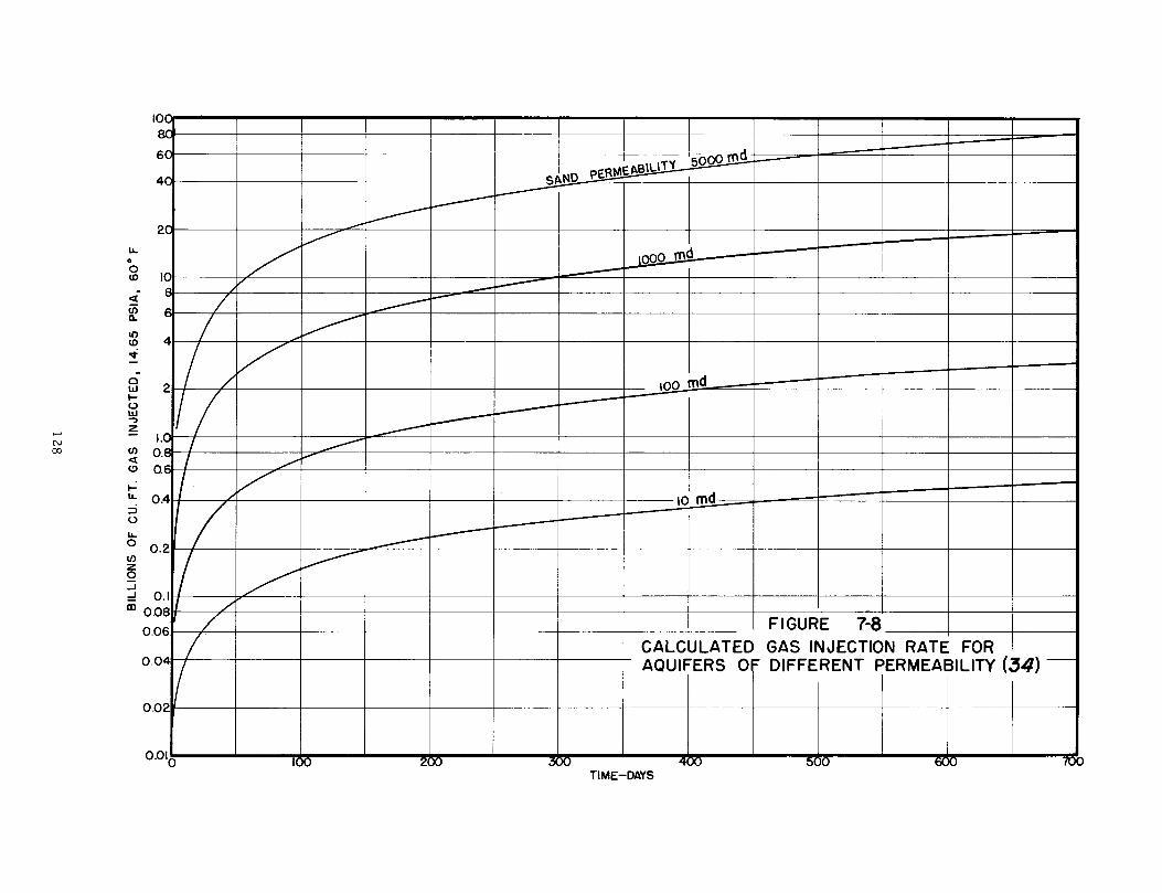

Initial Gas Injection
When an aquifer storage field is ready for gas injection, one would expect to have at
least two storage wells completed on top of the structure with water standing in these wells some-
where near the surface. How fast should gas be injected initially? Water moves relatively
slowly, and it will take time for gas to displace the water into the formation. It is recommended
that gas pressure be applied to the wellhead in 100 pounds per square inch increments with obser-
vation of the recession of the water level in the wellbore before increasing the gas pressure.
Once water is displaced from the wellbore, full gas injection pressure for depths of 1200 feet or
more could well be 100 to 150 pounds per square inch above the initial aquifer pressure. Sudden
increases in wellhead pressure with a full water column would increase the bottom hole pressure
almost instantaneously, running the risk of fracturing the reservoir rock by such practice. It
may take 2 or 3 days before the formation will begin to take gas at a rate equal to some 50 per
cent of its ultimate capacity,
Once gas injection has started, the neighboring observation well should show a pressure
response in a matter of hours and is likely to show the presence of gas in a few days. The initial
wafer of gas may be very thin, especially for layered systems. This means that during initial
gas injection, gas may-travel relatively great distances. This gas layer may travel down struc-
ture as much as 100 feet before the effects of gravity arrest the downward movement.
Figure 7-9 gives a view as to the mechanism by which gas enters the water bearing rock.
The instability of gas displacing water can be very great. Gas will preferentially enter the zone
with the highest permeability. Once gas starts moving into a zone, it will continue to flow because
the pressure transmits more easily through this gas layer than through the water layers due to
the differences in viscosity of water and gas, Figures 7-9b and 7-9c show how the gas waterinterface may be conceived to develop. Water retained in the layers between those containing gas
will drain down through the gas layers by a slow percolation process. Eventually the gas bubble
will develop a “bottom” but during high rates of injection, even in later years, the instability effects
may create a jagged interface between the gas bubble and the water zone.
Although only one well is shown in Figure 7-9, simultaneous injection may occur on a
group of wells. The practice is often followed of injecting into the second, third and fourth wells,
etc. only after the gas zone has reached the well in question. This, in effect, assures that only
one gas bubble is being created. It is expected that a series of separate bubbles simultaneously
created around a group of wells would eventually coalesce. However, in the early days, one can
conceive of some undue interference with water drainage patterns by having several gas layers.
In a matter of 1 to 3 years, the water in the sand at the “ceiling” of the reservoir will have drained
down to its residual content and the gas bubble will correspond to the structure of the cap rock.
Figure 7 -10 shows a sketch of an aquifer bubble after full coalescence has taken place
and much of the water has drained out. In effect, the gas bubble is now similar to a water drive
129

Figure 7-9 Development of Gas Bubble in an Aquifer.
gas field. When water is being pushed out, the gas water contact is concave downward (Figure
7-10a) since some head of water is required to move the water from the center of the bubble to
its periphery. The shape is concave upward (Figure 7-10b) upon gas withdrawal and water return.
Water Movement Calculations
The gas bubble in an aquifer storage project eventually reaches a stage where sufficient
data points are available to compare predicted and observed performance of the gas reservoir.
The geometric model used in evaluating the aquifer before gas injection would be the normal
130

Figure 7-10 Illustration of Bubble Bottom Shape for Aquifers.
starting point in such a comparison. After sufficient development has taken place, there are no
significant differences between predicting gas bubble pressure for a given injection-withdrawal
schedule for aquifer projects and naturally occurring water-drive gas fields used for gas storage.
A calculation method has recently been devised by Woods and Comer (70) for calculating the gas
bubble-aquifer behavior at early stages. The method has as yet been applied by the authors to
only one field. A brief discussion of this method is presented in Chapter 8 under the heading of
“Two Phase Flow. " The method of handling the growth of a gas bubble is also covered in Chapter
8 under the title of “The Moving Boundary Problem. "
131

Movement of Underground Water in Contact with Natural Gas
Pressure Gradients in Aquifers
In order to evaluate the applicability of the unsteady-state water movement equation to
the aquifer in question, one may compare observed pressures in the aquifer observation wells
with calculated pressures. These calculated pressures are determined from equations involving
the P D ( r D , Dt ) function tabulated in Appendices F and G.
The dimensionless pressure values tabulated in Appendices F and G are presented at
various discrete radii within the aquifer. The values of PD(rD,Dt ) in Appendix F for the constant
terminal rate case at rD = 1.0 are identical to the Pt function. That is, the Pt function simply
represents the dimensionless pressure at the inner boundary, rD = 1, in the same manner that
the P (rD D,tD) tables represent dimensionless pressures at other discrete values of the dimension-
less radius.
In Appendix G, for the constant terminal pressure case, the dimensionless pressure at
the inner boundary is always zero, with the initial dimensionless pressure (i. e., before drawdown)
equal to 1.0.
Example Problem 7-2: Calculation of Aquifer Pressure Gradient
Consider a gas bubble surrounded by a homogeneous, isotropic aquifer, with dimensions
and physical properties as follows:
r b = 2000 feet, radius at gas bubble edge
µ = 0.8 cp, water viscosity
= 0.1, porosity
= 7 x 1 0 - 6C vol/(vol)(psi), water plus formation compressibility
K = 1000 millidarcys, sand permeability
R = 100, so that the exterior boundary radius of the aquifer is 200,000 feet or about
38 miles.
If this gas bubble is maintained at 100 pounds per square inch above its initial pressure,
it is desired to find the time at which the effect of the exterior boundary becomes significant,
and to determine the pressure profile in the aquifer at and after this time.
First, the relation between actual and dimensionless time is found.
Now, from Appendix G, at R = 100, the dimensionless pressure begins to deviate from 1.0 at
r D = R = 100 at about tD = 103 or at 1000/2.83 days. Thus, the time at which the effect of
the exterior boundary becomes significant is approximately one year. Next, by plotting PD versus
132

tD with parameters of rD for R = 100, p(r,t) may be determined for one, two, three years, etc.
(See Figure 7-11). For example, after two years, at rD = 20, pD = 0.69. Thus, at a distance
of (20)(2000) = 40,000 feet (about 7.6 miles) from the center of the gas bubble, the pressure is
(1 - .69)(100) = 31 pounds per square inch above the initial pressure. Table 7-4 shows p(r,t) in
tabular form.
Table 7-4 p(r,t) For Example Problem
The pressure profile may then be plotted as in Figure 7-12.
In this analysis we assumed, for the purpose of simplification, that the gas bubble radius
was constant. In the actual case, of course, the gas bubble radius would be continually increasing
with time, so that the results obtained can only be considered as approximate values.
Location of Gas-Water Contact (Bubble Edge)
In the operation of gas storage reservoirs the gas-water interface moves in accordance
with the cyclic pressure schedule. In the case of aquifer storage reservoirs the interface con-
tinually advances downward and radially outward as the gas bubble is grown. This growth process
is ideally represented as shown in Figure 7-10. After an aquifer storage reservoir has been grown
for a period of time, it is desirable to determine, if possible, the radial extent of the gas bubble.
This knowledge allows conclusions concerning the approach of the gas to the spill point. The degree
of approach of a gas bubble to a water observation well is often desired.
The method described here of locating the interface requires that the gas bubble and aquifer
be approximately stablized at a constant pressure po, This can be accomplished by shutting in the
field after a period of growth and letting the pressure approach a constant value. The method
further requires an observation water well at a known distance r from the center of the gas bubble,
Figure 7-13. If after stabilization gas is injected to maintain the reservoir at a pressure ∆ p above
the stabilized value then a pressure reading at the water well at a known time after this initiation
of gas injection allows determination of the reservoir radius rb The method is equally applicable
when gas is produced to maintain a constant pressure drawdown of ∆ p.
The calculation of rb is a trial-and-error procedure involving use of the tabulated functionPD (rD,tD). This quantity is defined in terms of aquifer pressure as
(7-23)
133

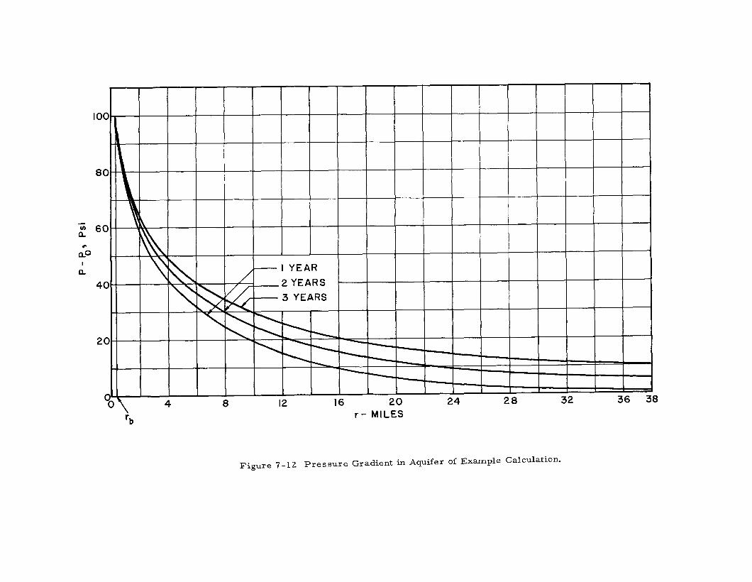
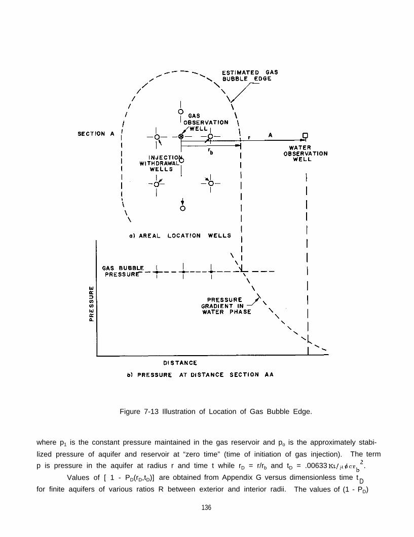
Figure 7-13 Illustration of Location of Gas Bubble Edge.
where p1 is the constant pressure maintained in the gas reservoir and po is the approximately stabi-
lized pressure of aquifer and reservoir at “zero time” (time of initiation of gas injection). The term
p is pressure in the aquifer at radius r and time t while rD = r/rb and tD = .00633
Values of [ 1 - PD(rD,tD)] are obtained from Appendix G versus dimensionless time t Dfor finite aquifers of various ratios R between exterior and interior radii. The values of (1 - PD)
136

in Appendix G are equally valid for infinite aquifers only at those times t D for which [ 1 - PD(rD,tD)]
= 1.0 ( or close to 1.0, e. g. 0.99 or 0.98). For example, the first seven rows of the table (Appendix
G) for R = 5.0 are applicable to an infinite aquifer since the effect of the exterior boundary is not felt
un t i l t D= 2.5, the eighth row down [ 1 - PD(5,2.5)] = . 9230 < 1.0. Since most practical prob-
lems will involve aquifers which are treated as infinite, care must be exercised in use of Appendix
G.
Calculation of rb requires the following procedure. After stabilization (shut-in) of reser-
voir and aquifer at an approximately constant pressure po, gas is injected ( or produced) to hold the
reservoir at a pressure p1, ∆ p above ( or below) po. After a period of time t, the pressure p in
a water observation well located r feet from the bubble center is read. Then from Equation 7-22
(7-24)
A value of rb is assumed and the dimensionless variables rD and tD are calculated as r/rb and
.00633 Kt/µ crb2. A sub-table of Appendix G is found such that PD(R,tD) is 0.98 or larger. The
value of PD(rD, Dt ) is then read from this sub-table and compared to the observed value calculated
from Equation 7-24. If the two PD values do not agree another rb must be assumed and the same
procedure repeated. Finally the PD values will agree for a certain assumed rb which is then the
answer.
Example Problem 7-3
An aquifer storage field is five years old. At the end of a two-month spring shut-in period
the reservoir and aquifer pressure approached a nearly constant value of 600 pounds per square
inch absolute. Beginning June 1, gas was injected to maintain the reservoir pressure at 750
pounds per square inch absolute. A water observation well 8000 feet from the center of the gas
bubble indicated a pressure of 648 pounds per square inch absolute on September 1. Locate the
approximate position (radius rb) of the gas-water contact.
Field Data
K = 325 millidarcys
c = 18 x 10-6 (vol)/vol)(psi)
µ = 1.05 centipoise
= 0 . 1 7
Solution
From Equation 7-23,
and
137

Movement of Underground Water in Contact with Natural Gas
Assumingr b = 2000 feet
r D = 8000/2000 = 4
tD =
From Appendix G, at R = 20, [1 - PD(20,25)] = 0.996
Since [ 1 - PD(20,14.4)] will be greater than [ 1 - PD(20,25)], the effect of the exterior
boundary (at R = 20) on values of [ 1 - P(r, 14.4)]R=2. is negligible and the values may be used
for an infinite aquifer. Interpolation yields
[ 1 - PD(4,14.4)] = 0.6827
so that the tabular value of (1 - PD) corresponding to rb = 2000 and the observed value are essen-
tially identical. Thus the reservoir radius is roughly 2000 feet.
In general, the values of P(rD, Dt ) used in the trial-and-error calculation will have to be
found by interpolation (or extrapolation) of the tabular values in rD and/or tD.
An alternate method is to plot the pressure gradient in the water phase through the observa-
tion well and find the intersection of the gas and water gradient curves as in Figure 7-13.
138

CHAPTER 8
SPECIAL TOPICS IN GAS STORAGE
Six special topics of interest in gas storage are given. The concept of using the summa-
tion of the pound-day products above and below the initial aquifer reservoir pressure as a guide
to water movement is presented. Methods of handling the moving boundary problem and the inter-
ference between two or more reservoirs on the same aquifer are treated. The importance of two
phase flow and stratified flow, neglected in most of the Monograph, is discussed.
Pound-Days as a Guide
Before reservoir calculations of water movement were made in gas storage operations,
water levels on observation wells adjacent to gas fields were found to rise and fall. High gas reser-
voir pressures caused water movement away from the bubble and the pressure rise in the observa-
tion well. Low gas reservoir pressures caused the water to return and the low observation well
pressures. It was reasoned that if the gas reservoir was at a pressure above the initial aquifer
value for a period of time and then below that value for a period of time such that the products of
“days at high pressure” times the “high pressure minus the initial aquifer value” and of “days at
low pressure " times the “difference between the low pressure and initial aquifer value” were equal,
then it was reasoned that there should be as much water returning to the gas reservoir during low
pressure as is pushed out during high pressure. By adding the daily gas bubble pressure as pounds
per square inch above (plus) or the pounds per square inch below (negative), the net pound-days is
obtained for an annual cycle. If the annual summation is negative, the gas bubble would be expected
to shrink due to water influx and if it were positive, the bubble would grow due to net water expul-
sion. Coats (6) and Katz et al (33) set up a series of calculations to establish the validity of the
above “rule of thumb” for estimating gas storage reservoir behavior.
The Moving Boundary Problem in Aquifer Storage
The data collected throughout the development of several aquifer storage projects duringrecent years have shown that the bubble first develops radially extending into an inverted saucer
shape geometry and then grows vertically while the water drains out from in-between the gas
streamers.
The radius of the gas bubble has been observed to increase from zero to nearly its maxi-
mum value during the early stages of bubble development. Due to this drastic change in location of
the gas-water interface the equations for various geometries with fixed boundaries become invalid.
The procedure given in the following, presented by Katz, Tek, and Jones (36), is developed to provide
approximate solutions to problems encountered in aquifer storage. It has been applied to the study
of three aquifer storage fields and found to give satisfactory results.
A gas bubble of small radius requires a higher pressure drop to maintain a given water
movement rate than one of larger radius. On the other hand, if one considers two gas bubbles of
139

Movement of Underground Water in Contact with Natural Gas
equal radii but subjected to different water rates, the one with the higher rate will require the
higher pressure drop. Consequently, during early phases of the development of aquifer storage
when the bubble radius is small, injection of gas at a given rate requires higher pressure drop
than later when the bubble is larger. On the basis of these arguments, it may be expected that a
given injection rate with a small radius should result in similar performance to higher injection
rate when the bubble is larger.
In order to account for the effect of changing radius on the pressure-production performance
of a storage field and still be able to apply the superposition principle, a concept of effective water
influx rate has been utilized. The following development is to be used in conjunction with the
resistance function method. However, in as much as a geometric model is employed in the develop-
ment of the resistance function, the use of such a model applies equally well here. For example,
the radial model (constant terminal rate case) may be used with the modifications presented below.
It is not necessary to have performance data available if K and At,r can be adequately estimated.
Whenever the radial model is employed, the AZ’s appearing in Equation 8-6, 8-7, 8-8, 8-9 are to
be replaced by Kr D P t .
An arbitrary reference gas bubble of radius rb* is first selected. A dimensionless time
tD * corresponding to rb* is calculated for each time step from:
(8-1)
Next a relation between the gas bubble volume and radius is assumed. Let the volume
corresponding to rb* be denoted as V* and the actual volume and radius at any time (n ∆ t) be Vn
and rb . The relation between the respective radii and volumes may be approximated by
(8-2)
where α is dependent upon the particular gas sand geometry. For instance, α = 1/2 for a dome of
parabolic shape; 2/3 for a hemispherical shape; 1 for a cylinder, etc. The selection of V* is
arbitrary. Experience has shown that the prediction of reservoir performance is insensitive to
the choice of V*. For convenience it may be chosen to be equal to one-half the largest volume
encountered in the “fit” of past performance data.
The dimensionless time corresponding to the actual radius at any time is given by:
(8-3)
The factor β n which modifies the water influx rate is given by:
140

Movement of Underground Water in Contact with Natural Gas
If we combine Equations 8-15 and 8-16 and rearrange, we obtain
(8-25)
However, the cumulative water influx, W en’ is equal to the change in the gas bubble volume
(8-26)
Thus(8-27)
Equation 8-27 may be substituted into Equation 8-25. The value of p can be solved from the result-ning equation. It appears as
where
Calculational Procedure
4.
5.
6.
7.
(8-28)
(8-29)
(8-30)
1. Select a value of α between 1/2 and 1.
2. Calculate from estimated field parameters,
3. Calculate V for time in At where n ∆ t should be at least 15 months, and
(8-35)
Recall that Sn = nnRT (Equation 6-8)
Starting with n = m + 1, calculate pn and Vn from Equation 8-28 and 8-35, where Bn and
Cn are calculated from Equations 8-29 and 8-37.
Compute the sum of the absolute deviation between the calculated and the observed bottom
hole pressures.
Repeat steps 2-5 for new values of K1 for a given α until the minimum deviation between
the observed and calculated pressures is found.
Repeat steps 1-6 for new values of α until the minimum deviation between observed and
calculated pressures is found.
144

Movement of Underground Water in Contact with Natural Gas
at large values of time.
Aside from the determination of β for each time step the calculation procedure for the
moving-boundary case is identical to the procedure outlined in detail in Chapter 6 for the field
boundary case. A field case study illustrating the procedure given above is presented in Chapter
11 for Field G.
Moving Boundary Approximations Based on Hemispherical Model
Another approximate method for treating reservoirs which are grown extensively through
the expulsion of water from its native formation can be derived using the hemispherical model.
The equation expressing the rate of water influx into the gas bubble at its exterior radius,
rb, is given in Chapter 3 by Equation 3-154. It appears as
If dimensionless time is large, Equation 8-12 may be approximated by
(8-12)
(8-13)
The cumulative water influx from time zero to time tn for a constant pressure drop, ∆ p, below the
equilibrium reservoir pressure, is given by integration of Equation 8-13
The integration is performed between the limits tm and tn rather than between t = 0 and tn , since
the assumption that is negligible is obviously invalid for small values of time. Conse-
quently, it is assumed that We , the cumulative water influx from the time of initiation of gas
injection until time tm , can be calculated from field data; i. e., field data are available for a
period of time. The method presented here cannot be applied before the storage project is initiated,
for example.
The terms rb and ∆ p in Equation 8-14 are now considered to vary with time instead of
being constants. Even though the integration of these variables is not a strictly valid operation,
application to field data has shown this to give a fair approximation. Accordingly, the replacementof the integral in Equation 8-14 by an approximately equivalent summation yields:
(8-15)
where
(8-16)
142

and rb may be considered to be the gas bubble radius at the beginning of the jth time interval when
time t = (j-1) ∆ t .
The radius rb can be related to the volume of the gas-in-place by a knowledge of the cap
rock geometry. If the cap rock is assumed conical (right-circular cone) then
where y is the distance between the apex of the cap rock and the gas-water interface and M is the
slope of the cap rock. The pore volume occupied by gas at time n ∆ t is
(8-18)
Similarly if the cap rock is assumed parabolic, then
(8-19)
and(8-20)
The pore volume can also be obtained using the gas law
(8-21)
Since we evaluate r at time t = (j - 1) ∆ t, then for a conical cap rock:
(8-22)
and for a parabolic cap rock:
(8-23)
Equations 8-22 and 8-23 may be generalized to allow for some intermediate cap rock geometry:
(8-24)
The values of Sf and α depend on the formation geometry. Some examples are shown in Table 8-1.
Table 8-1 Shape Factors and Exponents for Various Geometries
Cap Rock Geometry
Cylindrical
Conical
Parabolic
143
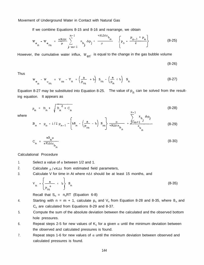
Movement of Underground Water in Contact with Natural Gas
If we combine Equations 8-15 and 8-16 and rearrange, we obtain
(8-25)
However, the cumulative water influx, W en’ is equal to the change in the gas bubble volume
(8-26)
Thus(8-27)
Equation 8-27 may be substituted into Equation 8-25. The value of p can be solved from the result-ning equation. It appears as
where
Calculational Procedure
4.
5.
6.
7.
(8-28)
(8-29)
(8-30)
1. Select a value of α between 1/2 and 1.
2. Calculate from estimated field parameters,
3. Calculate V for time in At where n ∆ t should be at least 15 months, and
(8-35)
Recall that Sn = nnRT (Equation 6-8)
Starting with n = m + 1, calculate pn and Vn from Equation 8-28 and 8-35, where Bn and
Cn are calculated from Equations 8-29 and 8-37.
Compute the sum of the absolute deviation between the calculated and the observed bottom
hole pressures.
Repeat steps 2-5 for new values of K1 for a given α until the minimum deviation between
the observed and calculated pressures is found.
Repeat steps 1-6 for new values of α until the minimum deviation between observed and
calculated pressures is found.
144

8. Using the optimum values of α and K1 and a projected gas inventory schedule, predict the
pressures using the equations employed in the fitting procedure.
The example calculation for Field F in Chapter 11 employs this procedure.
Interference Between Gas Fields
The water movement equations given in this Monograph have been discussed in relation
to a single reservoir situated on an aquifer. Situations exist, however, in which two or more
reservoirs are Located on a single aquifer. In these cases the pressure variations in a given
reservoir will be influenced by gas injection or production in the neighboring fields. That is,
pressure transients in the aquifer caused by operations in one field will travel through the aquifer
and “interfere” with or affect the pressure behavior of a neighboring field. For the sake of sim-
plicity, the remainder of this discussion deals with the case of two fields situated on a single
aquifer.
The pressure change (from initial reservoir pressure) in a field at any given time is a
sum of two components - the pressure change due to gas injection-production in that field and the
change caused by ooperations in the neighboring field. Thus for two fields designated as Field A
and Field B,
(8-36)
(8-37)
where po-pA p = pressure drop in Field A
(po - pA)A = pressure drop in Field A which would occur if Field B were non-existent
(PO- PA)B = pressure drop in Field A due to interference from Field B.
The terms in Equation 8-37 are analogously defined. The term (po - pA)A is calculated ignoringthe existence of Field B. Thus Field A pressures are calculated from Equation 5-21 to 5-24 and the
corresponding pore volumes are calculated from Equation 5-13. These pressures are denoted byp'A and V'Asince they are “uncorrected” or erroneous values in the respect that they must be modi-
fied by taking into account the interference from Field B. Similarly, Field B pressures and pore
volumes are calculated from the same equations ignoring the existence of Field A and are denoted
by p'B and V'B. At this point we have
and(8-38)
(8-39)
and have only to determine the interference effects (po - pA)B and (po-pB)A in order to calcu-
late the final “corrected” pressures pA and pB from Equations 8-36 and 8-37. Time subscripts
145
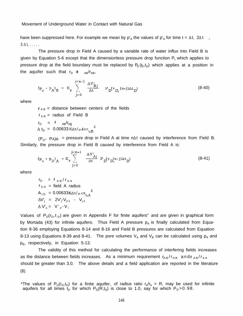
Movement of Underground Water in Contact with Natural Gas
have been suppressed here. For example we mean by p'A the values of p'A for time t = ∆ t, 2 ∆ t ,
3 ∆ t, . . . . .
The pressure drop in Field A caused by a variable rate of water influx into Field B is
given by Equation 5-6 except that the dimensionless pressure drop function Pt which applies to
pressure drop at the field boundary must be replaced by P (rD D,tD) which applies at a position in
the aquifer such that rD = AB/rbB,
(8-40)
where
A B = distance between centers of the fields
r b B = radius of Field B
rD = AB/rbB
∆ tD = 0.00633
(PO- PA)B = pressure drop in Field A at time n ∆ t caused by interference from Field B.
Similarly, the pressure drop in Field B caused by interference from Field A is:
where
(8-41)
rD = A B / r b A
r b A = field A radius
A t D = 0.00633
∆ V'j = 2V'j-Vj+1 - Vj-1
∆ V'o = V ' o - V i
Values of PD(rD, Dt ) are given in Appendix F for finite aquifers” and are given in graphical form
by Mortada (43) for infinite aquifers. Thus Field A pressure pA is finally calculated from Equa-
tion 8-36 employing Equations 8-14 and 8-16 and Field B pressures are calculated from Equation
8-13 using Equations 8-39 and 8-41. The pore volumes VA and VB can be calculated using pA and
pB, respectively, in Equation 5-13.
The validity of this method for calculating the performance of interfering fields increases
as the distance between fields increases. As a minimum requirement A B / r b B a n d A B / r b A
should be greater than 3.0. The above details and a field application are reported in the literature
(8).
*The values of PD(rD,tD) for a finite aquifer, of radius ratio re/rb = R, may be used for infiniteaquifers for all times tD for which PD(R,tD) is close to 1.0, say for which PD >0 .98 .
146
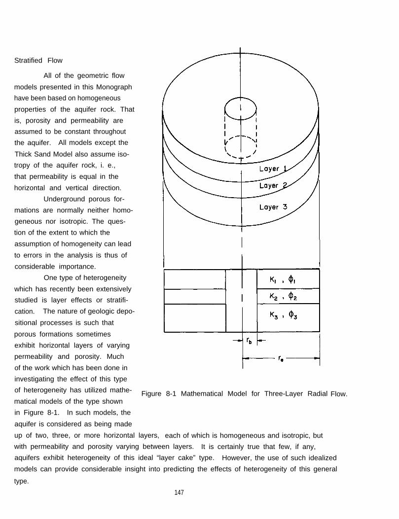
Stratified Flow
All of the geometric flow
models presented in this Monograph
have been based on homogeneous
properties of the aquifer rock. That
is, porosity and permeability are
assumed to be constant throughout
the aquifer. All models except the
Thick Sand Model also assume iso-
tropy of the aquifer rock, i. e.,
that permeability is equal in the
horizontal and vertical direction.
Underground porous for-
mations are normally neither homo-
geneous nor isotropic. The ques-
tion of the extent to which the
assumption of homogeneity can lead
to errors in the analysis is thus of
considerable importance.
One type of heterogeneity
which has recently been extensively
studied is layer effects or stratifi-
cation. The nature of geologic depo-
sitional processes is such that
porous formations sometimes
exhibit horizontal layers of varying
permeability and porosity. Much
of the work which has been done in
investigating the effect of this type
of heterogeneity has utilized mathe-
matical models of the type shown
in Figure 8-1. In such models, the
aquifer is considered as being made
up of two, three, or more horizontal
Figure 8-1 Mathematical Model for Three-Layer Radial Flow.
layers, each of which is homogeneous and isotropic, but
with permeability and porosity varying between layers. It is certainly true that few, if any,
aquifers exhibit heterogeneity of this ideal “layer cake” type. However, the use of such idealized
models can provide considerable insight into predicting the effects of heterogeneity of this general
type.
147

Movement of Underground Water in Contact with Natural Gas
When the layers of the system are entirely separated, as by shale layers, or when
vertical permeability is essentially zero, stratified system behavior is made up of the composite
of each individual layer, with no interlayer flow or "crossflow." In such cases, calculations of
the over-all system behavior may be made by applying single layer theory to each layer, and
summing the results. An analysis of stratified systems with separated layers has been presented
by Lefkovits, et al (39).
The system behavior and the mathematical analysis of performance become much more
complex for systems in which the layers are in communication over part or all of their common
interface. Pressure transients tend to be transmitted more rapidly in the higher permeability
layers. This effect leads to occurrence of vertical pressure gradients between layers which,
in turn, lead to interlayer fluid flow. The analysis of systems exhibiting such crossflow has been
the subject of several recent publications (2)(37)(39)(49)(53)( 54). Mathematical solutions are now
available for flow of a single slightly compressible fluid (such as water) in idealized “layer cake”
systems of any number of layers.
The primary conclusion derived from the work on stratified systems is that the behavior
of such systems can normally be computed with adequate accuracy using only single layer theory.
Except for a very short initial period, the transient performance of a system is essentially the
same as that of a homogeneous reservoir having mean properties. These mean properties are
computed from the permeability-thickness and porosity-thickness products, obtaining weighted
arithmetic average properties.
(8-42)
(8-43)
where Ki = permeability of layer “i”, millidarcys
= porosity of layer “i”, fraction
h 1 = thickness of layer “i”, feet
The underlying reason that stratified systems may be accurately treated in such a simple
manner is the large ratio between interlayer area and area at the gas-water interface. When
148

appreciable vertical permeability is present, the interlayer area is so large that the vertical
pressure transients are rapidly damped out due to interlayer flow.
A doctoral dissertation by Katz (37) contains analytical solutions and tables of results
for pressure distribution and fluid flux during constant-terminal-pressure depletion of two-layer
and three-layer systems with crossflow, together with tables of eigenvalues necessary in the
computations.
Two-Phase Flow
The flow equations presented to this point in the Monograph have been written for the
single phase flow of water in an aquifer. In no case have the equations involved the simultaneous
flow of two phases. All movements of a gas-water interface actually involve the simultaneous
flow of both gas and water. That is, near the gas-water interface, the pores are filled partly
with gas and partly with water, with both phases flowing simultaneously.
Analysis of the effects of two-phase flow in gas reservoir-aquifer problems is the sub-
ject of much recent and current research (35)(70). Little of this work has as yet led to develop-
ments which may be usefully incorporated into calculations of the type considered in this Mono-
graph. The subject will therefore be treated only briefly, by introducing some of the basic concepts.
The relative permeability concept is the basis for most multi-phase flow calculations.
The permeability of a porous medium to a fluid is at a maximum when the pores are completely
filled with that fluid. If a second fluid is introduced into the pore space, it tends, in a sense, to
block or constrict part of the flow passages for flow of the original fluid. The relative permea-
bility of a porous medium to a fluid is the ratio of the effective permeability to that fluid to the
absolute permeability of the porous medium obtained when all pores are filled with that fluid.
The effective permeabilities for each phase may be used with Darcy’s law to calculate the indi-
vidual flow rates for each fluid phase.
The phase saturation (i. e., fraction of pore space filled by that phase) is the most
important parameter in establishing the relative permeability of each fluid phase. Relative per-
meabilities are thus normally plotted as in Figure 8-2 which shows relative permeability to
both water and gas as a function of the per cent water saturation. This figure shows, for example,
that at a saturation of 50 per cent water and 50 per cent gas, relative permeability to gas is
15 per cent and relative permeability to water is 8 per cent. If the permeability to 100 per cent
gas or 100 per cent water is 1000 millidarcys, then the effective permeabilities are thus 150
millidarcys to gas and 80 millidarcys to water. In general, the sum of effective permeabilities
is not normally equal to the absolute permeability. Typical curves are given in the literature
(35)(44) for various porous media and fluid systems. Since these curves are often very dependent
on rock characteristics, they should be measured for each formation for which flow calculations
are to be made.
149

Movement of Underground Water in Contact with Natural Gas
The capillary pressure of a
porous medium reflects the inter-
facial forces between phases when
two fluids are present. These inter-
facial forces result in a pressure
difference across a fluid-fluid inter-
face within a pore. At a gas-water
interface within a pore, for example,
the pressure in the water phase may
be different from the pressure in
the immediately adjacent gas phase.
The capillary pressure for a porous
medium is normally plotted as in Fig-
ure 8-3, which shows the pressure
difference between phases as a func-
tion of water saturation for a typical
sandstone and a low permeability shale.
The capillary pressure at
100 per cent water saturation corres-
ponds to the threshold pressure for Figure 8-2 Typical Curve of Relative Permeability
displacement of water by gas at a Versus Water Saturation.
capillary discontinuity. Referring
to Figure 8-3, the gas pressure at the surface of a water filled rock must be raised to a value
of APl greater than the water pressure before any gas will begin to flow into the rock. Similarly,
at a sand-shale interface, where the shale is 100 per cent water filled, the gas pressure in the
sandstone must be raised to at least AP2 greater than the water pressure in the shale before gas
will begin to flow into the shale. Threshold pressures for sandstones are normally 10 pounds
per square inch or less, but may be several hundred pounds per square inch for cap rock shales.
All gas reservoir-aquifer systems, whether in water drive gas fields or in storage
projects, exhibit two-phase flow near the reservoir-aquifer boundary. As water encroaches into
the reservoir during pressure depletion, a saturation gradient is induced due to bypassing or
“trapping” of some gas by the encroaching water phase. Similarly, during gas injection, the
displacement of water by gas results in bypassing of water. A “twilight zone” of two-phase flow
is thereby created between the gas reservoir, which is usually at connate water saturation, and
the aquifer, which is initially 100 per cent water saturated. The net effect of this two-phase
zone is to somewhat decrease both gas and water permability near the reservoir-aquifer boundary.
This permeability reduction causes some damping of the pressure transients in this area, which
may cause some lag in actual pressure behavior compared with calculated pressures. Experience
150

Figure 8-3 Capillary Pressure Curves for Typical Sandstone and Shale.
has shown that this effect is small enough in developed fields so single phase flow calculations
can be used satisfactorily, and does not constitute a serious detriment to application of the
methods presented in this Monograph.
The most serious effects of two-phase flow occur during the early stages of development
of aquifer storage fields. In the initiation of such storage projects, gas is displaced into a sand
which is initially 100 per cent water saturated. The resultant displacement is not piston-like,
but results in formation of significant saturation gradients in the vicinity of the gas injection
well or wells.
The manner in which gas enters the aquifer upon initiation of an aquifer storage project
may be dependent on the homogeneity of the aquifer sand. The Mt. Simon sand, for example,
frequently exhibits some degree of permeability stratification. Initial gas injection into this
sand has been observed to result in formation of thin gas “wafers” which propagate rapidly through
the more permeable layers. This type of behavior has been considered in some detail in Chapter
7. Gas injection into an aquifer in the St. Peter formation has been reported (70) to result in a
more uniform vertical saturation distribution during initial displacement.
151
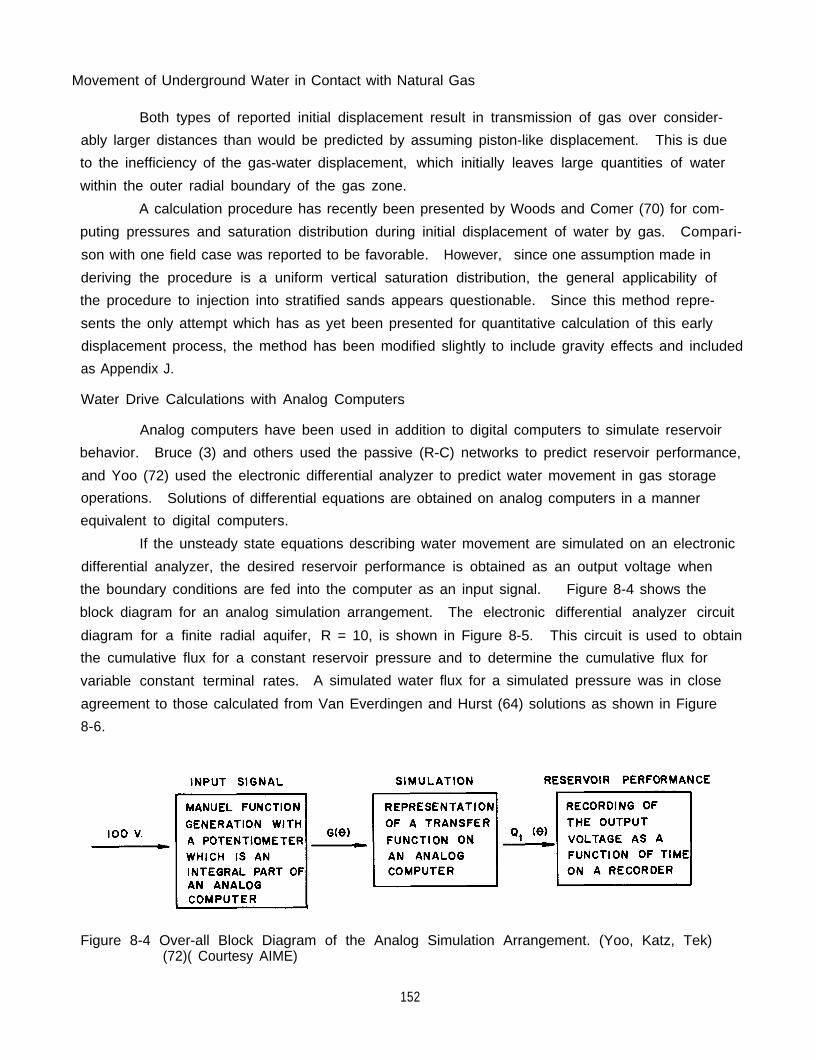
Movement of Underground Water in Contact with Natural Gas
Both types of reported initial displacement result in transmission of gas over consider-
ably larger distances than would be predicted by assuming piston-like displacement. This is due
to the inefficiency of the gas-water displacement, which initially leaves large quantities of water
within the outer radial boundary of the gas zone.
A calculation procedure has recently been presented by Woods and Comer (70) for com-
puting pressures and saturation distribution during initial displacement of water by gas. Compari-
son with one field case was reported to be favorable. However, since one assumption made in
deriving the procedure is a uniform vertical saturation distribution, the general applicability of
the procedure to injection into stratified sands appears questionable. Since this method repre-
sents the only attempt which has as yet been presented for quantitative calculation of this early
displacement process, the method has been modified slightly to include gravity effects and included
as Appendix J.
Water Drive Calculations with Analog Computers
Analog computers have been used in addition to digital computers to simulate reservoir
behavior. Bruce (3) and others used the passive (R-C) networks to predict reservoir performance,
and Yoo (72) used the electronic differential analyzer to predict water movement in gas storage
operations. Solutions of differential equations are obtained on analog computers in a manner
equivalent to digital computers.
If the unsteady state equations describing water movement are simulated on an electronic
differential analyzer, the desired reservoir performance is obtained as an output voltage when
the boundary conditions are fed into the computer as an input signal. Figure 8-4 shows the
block diagram for an analog simulation arrangement. The electronic differential analyzer circuit
diagram for a finite radial aquifer, R = 10, is shown in Figure 8-5. This circuit is used to obtain
the cumulative flux for a constant reservoir pressure and to determine the cumulative flux for
variable constant terminal rates. A simulated water flux for a simulated pressure was in close
agreement to those calculated from Van Everdingen and Hurst (64) solutions as shown in Figure
8-6.
Figure 8-4 Over-all Block Diagram of the Analog Simulation Arrangement. (Yoo, Katz, Tek)(72)( Courtesy AIME)
152

Figure 8-5 LM10 (Electronic Differential Analyzer) Circuit Diagram for R = 10 to Get Cumula-tive-Flux Function. (Yoo, Katz, and Tek)(72)(Courtesy AIME)
153

-Pressure Case,Figure 8-6 Comparison of the Analog Result with Theoretical Value to a ConstantR= 10. (Yoo, Katz, and Tek)(72)(Courtesy AIME)
154
CHAPTER 9
DEMONSTRATION OF ALL METHODS ON FIELD A
The working equations for calculating water movement have been presented in previous
chapters for four geometric models and the generalized performance method. Since numerous
steps are involved in the application of these methods to a case study, an example demonstrating
the applications of the equations on Field A is presented in this chapter. These calculations
involve the determination of the initial gas pore volume, the optimum coefficient Kr or Kp, and
the prediction of reservoir pressures for a given gas injection-production schedule. For the pur-
pose of comparison, the pressures assuming no water movement are predicted. Thus the follow-
ing analysis of Field A is presented as a complete case study. The application of all geometric
models to a single field might be questioned. However, in this instance it seemed to be the best
way of presenting example calculations.
Field A is an old depleted gas reservoir converted to storage operations. The discovery
pressure was 520 psig (wellhead) and the original reserves were 24,264,356 thousand cubic feet
(60°F and 14.65 pounds per square inch absolute) of gas.
Prior to conversion to gas storage, the field had been shut in for several years. Water
had encroached on the depleted areas of the field successively drowning out the lower-lying proper-
ties. The pressure recovered to 408 pounds per square inch gauge due to this water encroachment.
Field reserves when converted to storage are estimated at 1,000,000 thousand cubic feet. These
conditions are used as a pseudo initial condition for analysis of the gas storage operations.
Geology and Field Data
The gas-bearing sand, uniform in texture and composed of round, medium-sized grains,
is an anticlinal structure. The sand body grades up-dip to the northeast into shaley sand and shales
which confines the gas, while to the south the sand extends a considerable distance beyond the
southern limit of the field. Thick shale beds above the sand form an effective caprock. The sand
rests directly upon the Mississippi Lime throughout most of the field except in a few wells where a
thin shale streak is found. A plan sketch of the field is shown in Figure 9-1,
The reservoir and aquifer properties are given in Table 9-1l and the production-pressure
history tabulated in Table 9-2.
The Problem
Given the data on Field A, compute the reservoir pressures for the production-injection
schedule. It is suggested that about one-third of the data to be used in devising the calculation pro-
cedure and the pressure data for the last two-thirds of the time be reserved for comparing computed
versus actual field data.
155
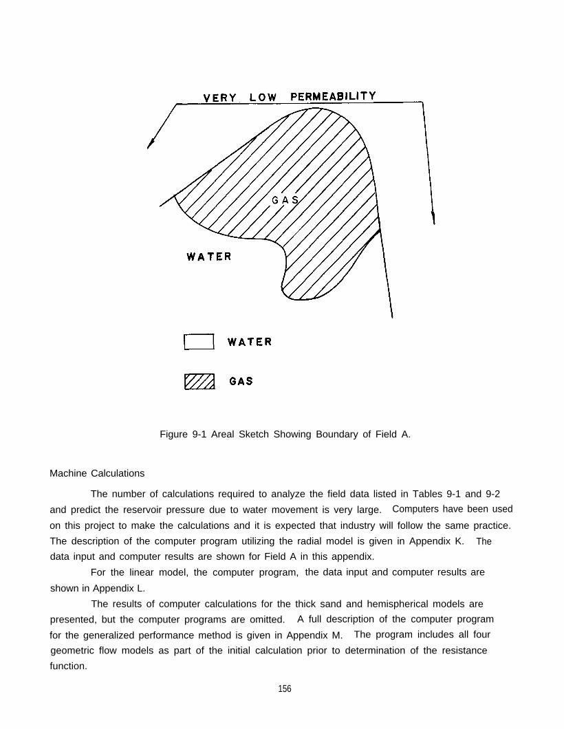
Figure 9-1 Areal Sketch Showing Boundary of Field A.
Machine Calculations
The number of calculations required to analyze the field data listed in Tables 9-1 and 9-2
and predict the reservoir pressure due to water movement is very large. Computers have been used
on this project to make the calculations and it is expected that industry will follow the same practice.
The description of the computer program utilizing the radial model is given in Appendix K. The
data input and computer results are shown for Field A in this appendix.
For the linear model, the computer program, the data input and computer results are
shown in Appendix L.
The results of computer calculations for the thick sand and hemispherical models are
presented, but the computer programs are omitted. A full description of the computer program
for the generalized performance method is given in Appendix M. The program includes all four
geometric flow models as part of the initial calculation prior to determination of the resistance
function.
156

Table 9-1 Storage Field A, Reservoir Data
157
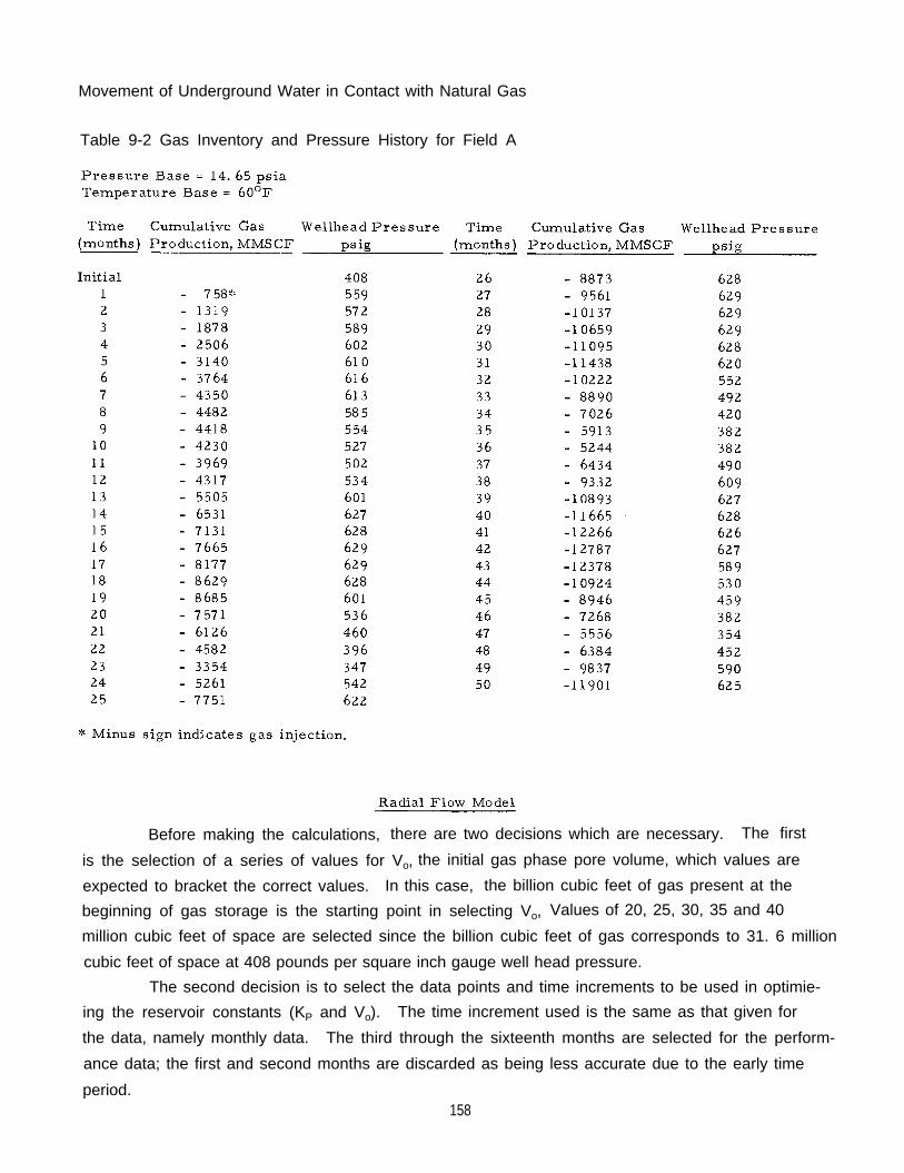
Movement of Underground Water in Contact with Natural Gas
Table 9-2 Gas Inventory and Pressure History for Field A
Before making the calculations, there are two decisions which are necessary. The first
is the selection of a series of values for Vo, the initial gas phase pore volume, which values are
expected to bracket the correct values. In this case, the billion cubic feet of gas present at the
beginning of gas storage is the starting point in selecting Vo, Values of 20, 25, 30, 35 and 40
million cubic feet of space are selected since the billion cubic feet of gas corresponds to 31. 6 million
cubic feet of space at 408 pounds per square inch gauge well head pressure.
The second decision is to select the data points and time increments to be used in optimie-
ing the reservoir constants (KP and Vo). The time increment used is the same as that given for
the data, namely monthly data. The third through the sixteenth months are selected for the perform-
ance data; the first and second months are discarded as being less accurate due to the early time
period.158
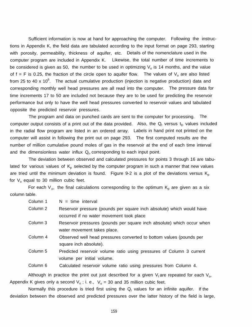
Sufficient information is now at hand for approaching the computer. Following the instruc-
tions in Appendix K, the field data are tabulated according to the input format on page 293, starting
with porosity, permeability, thickness of aquifer, etc. Details of the nomenclature used in the
computer program are included in Appendix K. Likewise, the total number of time increments to
be considered is given as 50, the number to be used in optimizing Vo is 14 months, and the value
of f = F is 0.25, the fraction of the circle open to aquifer flow.
from 25 to 40 x 106.
The values of Vo are also listed
The actual cumulative production (injection is negative production) data and
corresponding monthly well head pressures are all read into the computer. The pressure data for
time increments 17 to 50 are included not because they are to be used for predicting the reservoir
performance but only to have the well head pressures converted to reservoir values and tabulated
opposite the predicted reservoir pressures.
The program and data on punched cards are sent to the computer for processing. The
computer output consists of a print out of the data provided. Also, the Qt versus tD values included
in the radial flow program are listed in an ordered array. Labels in hand print not printed on the
computer will assist in following the print out on page 293. The first computed results are the
number of million cumulative pound moles of gas in the reservoir at the end of each time interval
and the dimensionless water influx Qt, corresponding to each input point.
The deviation between observed and calculated pressures for points 3 through 16 are tabu-
lated for various values of Kp selected by the computer program in such a manner that new values
are tried until the minimum deviation is found. Figure 9-2 is a plot of the deviations versus Kp
for Vo equal to 30 million cubic feet.
For each Vo, the final calculations corresponding to the optimum Kp are given as a six
column table.
Column 1 N = time interval
Column 2 Reservoir pressure (pounds per square inch absolute) which would have
occurred if no water movement took place
Column 3 Reservoir pressures (pounds per square inch absolute) which occur when
water movement takes place.
Column 4 Observed well head pressures converted to bottom values (pounds per
square inch absolute).
Column 5 Predicted reservoir volume ratio using pressures of Column 3 current
volume per initial volume.
Column 6 Calculated reservoir volume ratio using pressures from Column 4.
Although in practice the print out just described for a given Vt are repeated for each Vo,
Appendix K gives only a second Vo ; i. e., Vo = 30 and 35 million cubic feet.
Normally this procedure is tried first using the Qt values for an infinite aquifer. If the
deviation between the observed and predicted pressures over the latter history of the field is large,
159
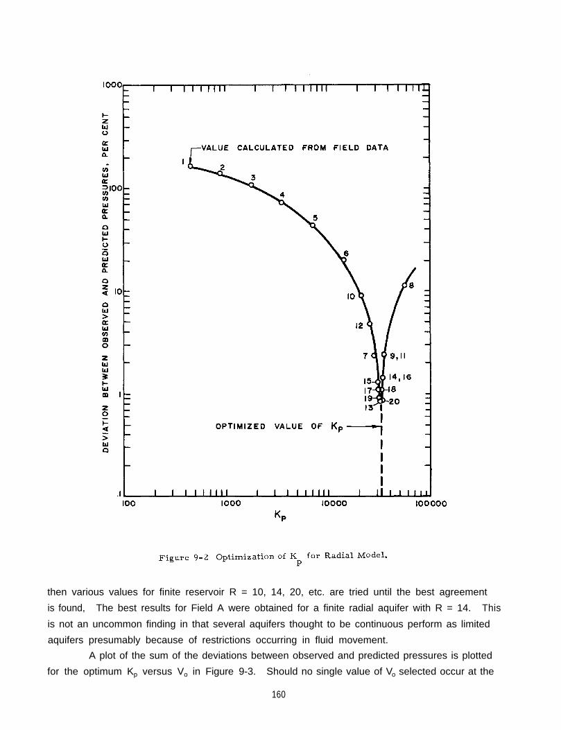
then various values for finite reservoir R = 10, 14, 20, etc. are tried until the best agreement
is found, The best results for Field A were obtained for a finite radial aquifer with R = 14. This
is not an uncommon finding in that several aquifers thought to be continuous perform as limited
aquifers presumably because of restrictions occurring in fluid movement.
A plot of the sum of the deviations between observed and predicted pressures is plotted
for the optimum Kp versus Vo in Figure 9-3. Should no single value of Vo selected occur at the
160

Figure 9-3 Determination of Initial Gas Pore Volume.
minimum, a new value or values could be put into the computer until one of the print out corres-
ponds to a satisfactory Vo,
The computed performance of the reservoir is presented on Figures 9-4, 9-5 and 9-6.
Figure 9-4 presents the computed pressures which would have occurred without water movement
in the 30 million cubic feet of initial space. Figure 9-5 compares actual and predicted reservoir
pressures for times 17 through 50 at the optimum selection of Vo and Kp. Figure 9-6 is a com-
parison of the ratios of pore volume computed from field data; i.e., reservoir pressures and
gas volumes with pore volumes predicted from water movement.
Calculations Performed by Computer
At this time, the gap will be bridged between the developments of equations in the earlier
chapters and the completed computer program. This discussion should assist in understanding
the computer program given in Appendix K and will illustrate some of the hand calculations which
the engineer may wish to do as a check on the computer solution. In general, calculations will be
161
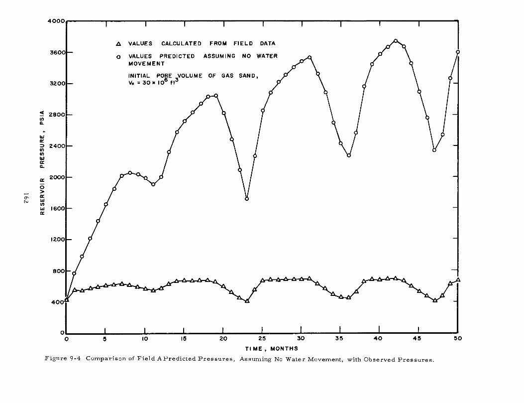


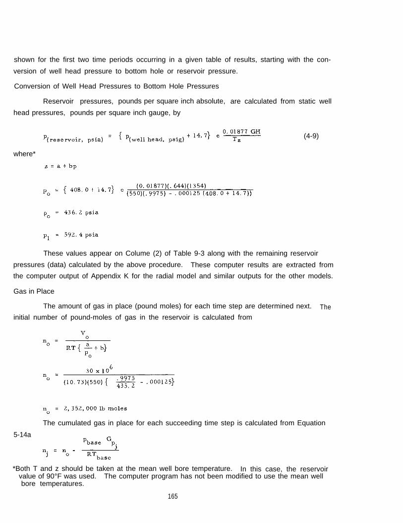
shown for the first two time periods occurring in a given table of results, starting with the con-
version of well head pressure to bottom hole or reservoir pressure.
Conversion of Well Head Pressures to Bottom Hole Pressures
Reservoir pressures, pounds per square inch absolute, are calculated from static well
head pressures, pounds per square inch gauge, by
(4-9)
where*
These values appear on Colume (2) of Table 9-3 along with the remaining reservoir
pressures (data) calculated by the above procedure. These computer results are extracted from
the computer output of Appendix K for the radial model and similar outputs for the other models.
Gas in Place
The amount of gas in place (pound moles) for each time step are determined next. Theinitial number of pound-moles of gas in the reservoir is calculated from
The cumulated gas in place for each succeeding time step is calculated from Equation
5-14a
*Both T and z should be taken at the mean well bore temperature. In this case, the reservoirvalue of 90°F was used. The computer program has not been modified to use the mean wellbore temperatures.
165

Movement of Underground Water in Contact with Natural Gas
Table 9-3 Calculated Values for Field A Using Geometric Flow Models
166
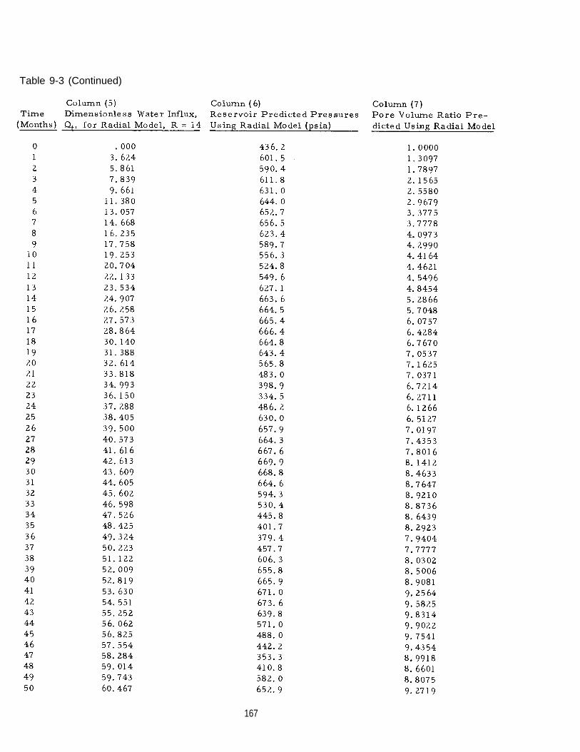
Table 9-3 (Continued)
167

Movement of Undergraduate Water in Contact with Natural Gas
Table 9-3 (Continued)
168

Table 9-3 (Continued)
169

Movement of Underground Water in Contact with Natural Gas
Thus
and
These values along with the remaining values for the gas inventory are tabulated in
Column (3) of Table 9-3.
Radius of the Bubble
The radius of the gas bubble or field is calculated from
(4-8)
This radius is printed out as one of the results
Dimensionless Time
Dimensionless time values at each time step are given by
where
This At, is printed out with the results.
(2-10)
Therefore
tD(1) = 1(3.603) = 3.603
tD(2) = 2(3.603) = 7.206
tD(3) = 3(3.603) = 10.809
etc.
These values are not printed out.
These values are used in the application of the working equations for all models.
Pressures for No Water Movement
The reservoir pressures for no water movement can be predicted from the gas law:
(9-1)
170

p2 = 998.3 psiaThese results along with the predicted pressures for the remaining time intervals are
tabulated in Column (4) in Table 9-3 and are plotted on Figure 9-4.
Predicted Reservoir Pressure
The application of the radial model water flow equation will be demonstrated for a
finite aquifer, R = 14, using the Working Equation 5-21 obtained from the superposition of the
radial flow Equation 2-11, constant terminal pressure case.
The values of dimensionless water influx Q.j ∆ t D are interpolated from Appendix D for
R = 14 for the corresponding value of dimensionless time and are listed in Table 9-3, Column (5).
The pressures are predicted by the following equations:
The remaining pressures are calculated by
where
171
(5-26)
(5-27)
(5-28)
(5-26)

(5-27)
(5-28)
where
p2 = 590.4 psia
These cornpouted results and the remaining values of the predicted pressures are given
on Column (6) in Table 9-3 and plotted in Figure 9-5.
Pore Volume
The pore volume ratio, the ratio of the current pore volume to the initial pore volume,
is calculated from
(9-2)
Thus
and
These results and the pore volume ratios for the remaining time intervals are given in
Table 9-3, Column (7) and plotted in Figure 9-6.
172
Movement of Underground Water in Contact with Natural Gas

Flow Diagram
The details of the computer program development are shown by the flow diagram in
Appendix K. This diagram should be sufficient to guide the writing of a program in any language.
For those who wish to follow the MAD language, a Computer Primer for the MAD Language by
E. I. Organick is available at Ulrichs Book Store, 549 East University, Ann Arbor, Michigan,
Linear Flow Model
The two preliminary decisions, the selection of Vo and time increments used in optimiz-
ing the values of Kp, made prior to the application of the radial model must also be made before
the linear program can be used. The same values were selected in this program as were used
in the radial model. In addition to the reservoir information used in the radial model, the width
of the aquifer must be known. For the linear model, tables of dimensionless water influx, Qt,
and dimensionless time, t D’ are omitted since Qt is calculated directly from tD, Except for these
minor changes, the use of the linear flow model is identical to the radial model. The description
of the computer program for the linear model is given in Appendix L. Since the flow diagram for
the linear model is similar to the radial model, it is not included in this appendix.
Again the sum of the deviation between observed and calculated pressures was calculated
for various values of Kp’ selected by the program for each value of initial pore volume. Kp‘,
defined by
(9-2)
is used by the linear computer program to facilitate the calculations. A plot of pressure deviation
versus Kp’ is given in Figure 9-7. The initial gas pore volume, Vo = 30 x 106 cubic feet was
used in these calculations. The optimum value of Kp’ is 209,000.
Except for the calculation of reservoir pressures for water movements, the calculations
in the linear model are identical to the calculations in the radial model. Thus the calculations for
reservoir bottom holes pressures, gas in place, dimensionless time, and pressure for no water
movement will not be repeated.
The application of the working Equation 5-26, 5-27, and 5-28 to predict the field perform-
ance of Field A using the linear model can be further simplified for machine calculations. These
working equations are
(5-26)
(5-27)
173

(5-28)
where the values of Kp and Qt for the linear model are given in Table 5-1 as Kp = 1.13 cA and
where j is the number of time intervals. If Kp’ is defined as Kp’ =
then Equations 5-27 and 5-28 can be rewritten for the linear flow
model as
174

and
(9-3)
(9-4)
The pressures are predicted using Equations 5-26, 9-3, and 9-4.
where
175
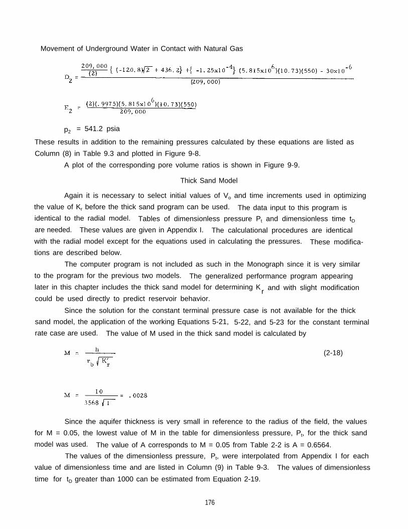
Movement of Underground Water in Contact with Natural Gas
p2 = 541.2 psia
These results in addition to the remaining pressures calculated by these equations are listed as
Column (8) in Table 9.3 and plotted in Figure 9-8.
A plot of the corresponding pore volume ratios is shown in Figure 9-9.
Thick Sand Model
Again it is necessary to select initial values of Vo and time increments used in optimizing
the value of Kr before the thick sand program can be used. The data input to this program isidentical to the radial model. Tables of dimensionless pressure Pt and dimensionless time tDare needed. These values are given in Appendix I. The calculational procedures are identical
with the radial model except for the equations used in calculating the pressures. These modifica-tions are described below.
The computer program is not included as such in the Monograph since it is very similar
to the program for the previous two models. The generalized performance program appearing
later in this chapter includes the thick sand model for determining Kr and with slight modification
could be used directly to predict reservoir behavior.
Since the solution for the constant terminal pressure case is not available for the thick
sand model, the application of the working Equations 5-21, 5-22, and 5-23 for the constant terminalrate case are used. The value of M used in the thick sand model is calculated by
(2-18)
Since the aquifer thickness is very small in reference to the radius of the field, the values
for M = 0.05, the lowest value of M in the table for dimensionless pressure, Pt, for the thick sand
model was used. The value of A corresponds to M = 0.05 from Table 2-2 is A = 0.6564.
The values of the dimensionless pressure, Pt, were interpolated from Appendix I for each
value of dimensionless time and are listed in Column (9) in Table 9-3. The values of dimensionless
time for tD greater than 1000 can be estimated from Equation 2-19.
176

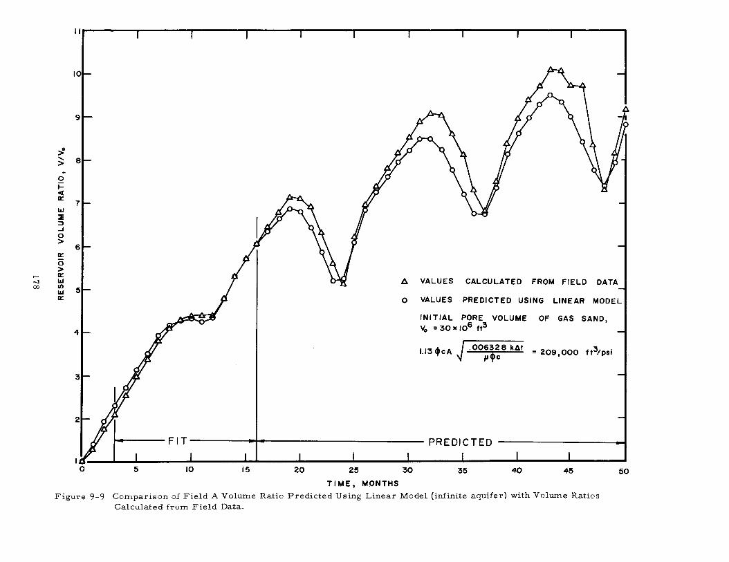
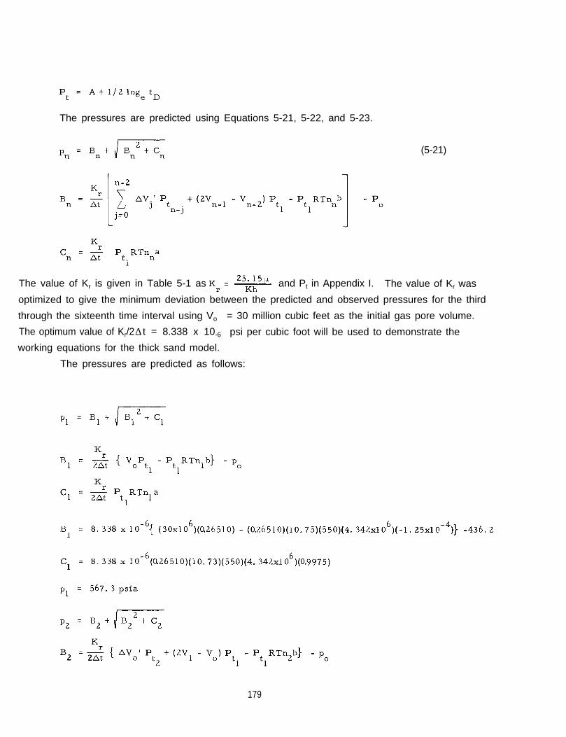
The pressures are predicted using Equations 5-21, 5-22, and 5-23.
(5-21)
The value of Kr is given in Table 5-1 as and Pt in Appendix I. The value of Kr was
optimized to give the minimum deviation between the predicted and observed pressures for the third
through the sixteenth time interval using Vo
The optimum value of Kr/2 ∆ t = 8.338 x 10-6
= 30 million cubic feet as the initial gas pore volume.
psi per cubic foot will be used to demonstrate the
working equations for the thick sand model.
The pressures are predicted as follows:
179

Movement of Underground Water in Contact with Natural Gas
p2 = 595.1 psia
The remaining values are tabulated in Column (10) of Table 9-3 and plotted in Figure
9-10. The corresponding pore volume ratio versus time is shown in Figure 9-11.
Hemispherical Model
As in the previous geometric models, the values of initial pore volume Vo and time
increments used in optimizing Kp are selected prior to the use of the hemispherical model. The
data input with the hemispherical model is identical to the radial model data input except the
tables of dimensionless water influx, Qt, and dimensionless time, t D’ are deleted since Qt can
be calculated directly from tD. Modifications in the equations for calculating the reservoir pres-
sure pressures are presented below.
The working Equations 5-26, 5-27, and 5-28 are used to predict the performance of
Field A using the hemispherical model. These equations are
(5-27)
(5-28)
where the values for Kp and Qt for the hemispherical model are given in Table 5-1 as Kp =
6.28 rb3 c and Qt = tD t 2 where tD = The value of Kp given in Table 5-1
180


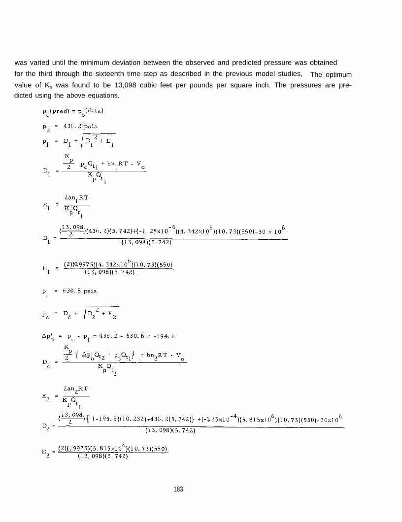
was varied until the minimum deviation between the observed and predicted pressure was obtained
for the third through the sixteenth time step as described in the previous model studies, The optimumvalue of Kp was found to be 13,098 cubic feet per pounds per square inch. The pressures are pre-dicted using the above equations.
183

Movement of Underground Water in Contact with Natural Gas
p 2 = 627.7 psia
This value and the remaining values of the predicted pressure are given in Column (12)
of Table 9-3 and plotted in Figure 9-12. The corresponding pressures are given in Figure 9-13.
Generalized Performance Method Using Resistance Function
The three parts involved in the application of the resistance function method are illustrated
below. These parts are: (1) The fit of an appropriate flow model to the early-time data through
optimization of Kr. The use of the radial model for an infinite aquifer is illustrated. As pointed
out in Chapter 6, the Constant Terminal Rate Case is used in conjunction with the resistance func-
tion. (2) The second part illustrated is the generation of the resistance function curve directly
from field data. Restrictions placed on AZ’s prevent wild oscillations. (3) The final step is
the extrapolation of the curve for field performance predictions in the future. The computer pro-
gram is presented in Appendix M. It is necessary to solve parts (1) and (2) on the computer, per-
form a manual extrapolation of the resistance function, and submit the program with the extrapola-
tion for calculating item (3).
Obtaining Kr From Early Data
The radial model is employed to determine the best value for Kr using the third through
the sixteenth time increments or months. It is necessary to know the initial pore volume Vo. A
value of 30 million cubic feet is used in this case. The input data and calculation procedures are
essentially identical with those used in optimizing K in the calculations with the radial flow model.P
The computer program described in Appendix M includes the example calculation for Field A.
Starting on page 299, the data input are listed including such items as pressure base
(14. 65 psia), temperature base (520°R), depth of well 1354 feet, gas gravity (0.644), reservoir
temperature (550ºR), gas compressibility constants a and b, and the number of time steps (26).
The well head pressures (psig) and corresponding cumulative gas production (injection is negative)
are given in ordered arrays. Model 1, the radial model is selected. Alternates could have been
the thick sand model (2) or the linear model (3). The comparison of observed and calculated pres-
sures is made for the third through sixteenth months.
The program provides for a print out of the data dimensionless times and pressures, and
the Kr and corresponding deviation between observed and calculated pressures for a series of twenty
trials. The optimum Kr is found by the computer as 2.7262 x 10⁻⁴ , Figure 9-14 is a plot of the
deviations showing optimum Kr Using the optimum Kr, the computer proceeds to compute (2)
the resistance function for the first sixteen time periods. From the field data the (Z’s) are com-
puted for time periods 17 through 26, step 2. Figure 9-15 is a plot of the resistance function (Z) versus
time.
184


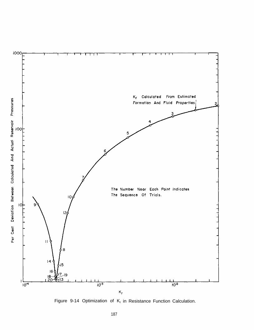
Figure 9-14 Optimization of Kr in Resistance Function Calculation.
187

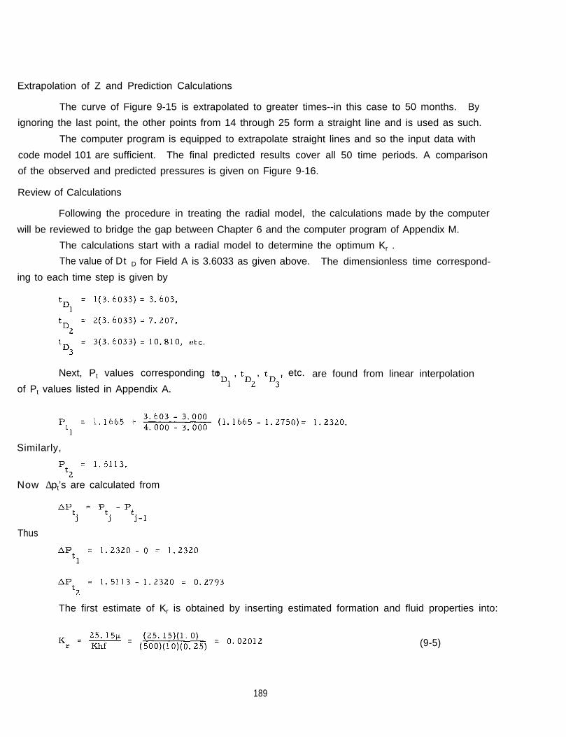
Extrapolation of Z and Prediction Calculations
The curve of Figure 9-15 is extrapolated to greater times--in this case to 50 months. By
ignoring the last point, the other points from 14 through 25 form a straight line and is used as such.
The computer program is equipped to extrapolate straight lines and so the input data with
code model 101 are sufficient. The final predicted results cover all 50 time periods. A comparison
of the observed and predicted pressures is given on Figure 9-16.
Review of Calculations
Following the procedure in treating the radial model, the calculations made by the computer
will be reviewed to bridge the gap between Chapter 6 and the computer program of Appendix M.
The calculations start with a radial model to determine the optimum Kr .
The value of D t D for Field A is 3.6033 as given above. The dimensionless time correspond-
ing to each time step is given by
Next, Pt values corresponding to , , , etc. are found from linear interpolation
of Pt values listed in Appendix A.
Similarly,
Now ∆ pt’s are calculated from
Thus
The first estimate of Kr is obtained by inserting estimated formation and fluid properties into:
189
(9-5)


It is convenient at this point to compute values of Sn/ ∆ t, where
(9-6)
for n = 0, 1, 2,. , . . i, where i denotes the time step corresponding to the last available data. For
purposes of illustration assume that the last known’ data falls on the twenth-sixth month following
initiation of the project, (i.e., i = 26). The value of Vo = 30 million cubic feet was obtained from
estimated gas reserves in the field. This value will be used as a first guess for the following
computations. These values are found on page 305 of Appendix M.
The remaining Sn/ ∆ t values are listed in Table 9-4.
Table 9-4 Values of Sn/ ∆ t
1 9 1

Movement of Underground Water in Contact with Natural Gas
The next step involves calculation of p1, ew1 , then p2, ew2, . . . . p16, ew16 using the equa-
tions for the radial flow model, constant terminal rate case, and the value of Kr determined above.These calculated pressures are compared to the actual (data) reservoir pressures. The per centdeviation is determined from the absolute value of the difference between the two pressures:
(9-7)
Figure 9-14 shows the initial estimate of the value of Kr ( = 0.02012) and the correspond-
ing percentage deviation between calculated and observed static bottom-hole pressures in the gas
bubble. Only pressures corresponding to time steps 3,4, 5. . . , 16 were used for the computation
of the per cent deviation. The first two pressure-data points were considered to be least accurate
and were disregarded in the comparison.
According to the algorithm of the computer program optimizing routine shown in the flow
diagram of Appendix M, the next assumed value of Kr is twice the original value or 0.04024. The
resulting deviation for this Kr is shown in Figure 9-14, as point “2”. Subsequent trials are indi-
cated by the numbers appearing adjacent to the points in Figure 9-14.
twentieth trial is 2,7262 x 10⁻⁴.
It is seen that Kr for the
The computation of p1, ew1; . . . . p16, ewl6 using this value of K rwill be illustrated.
According to Equation 6-10
where
and
p1 = 567.1 psia
The water influx rate is obtained from Equation 6-13:
192

Next calculate p3, ew3, then p4, ew4, etc. The values appear as the initial values of the computer
print out on page 304.
Calculate the percentage deviation:
% deviation =
Figure 9-14 shows this value to be near the minimum deviation. Therefore 2.7262 x 10 - 4
used in
193

Movement of Underground Water in Contact with Natural Gas
the calculation of these pn values will be taken as (K )r optimum’The AZ’s, according to Equation 6-18, for the initial portion of the fit are
∆ Z n = (K r)op t imum ∆ P t n
∆ Z1 = 2.7262 x 10 - 4 x 1.2320 = 3.3586 x 10⁻⁴
∆ Z2 2.7262 10 - 4= x x 0.2793 = 0.7614 x 10⁻⁴
The remaining values, out to ∆ Z 1 6 , are listed in the computer printout.
Generation of the Z-Curve Using Field Data
The next steps consist of computing ∆ Z 1 7 (17 = m +1), then forcing it to lie within the
inequalities (6-24), calculating P17, and ew17, and then repeating the process for n = 18, etc.
Let = 0.02. The inequality (6-24) states that ∆ Z17 must lie between the limits:
or
Thus 1.808 x 10⁻⁵ is too high and ∆ Z 1 7 is set equal to 0.891 x 10⁻⁵, Now, using this modified
value of ∆ Z17, p17 can be calculated from
where
194
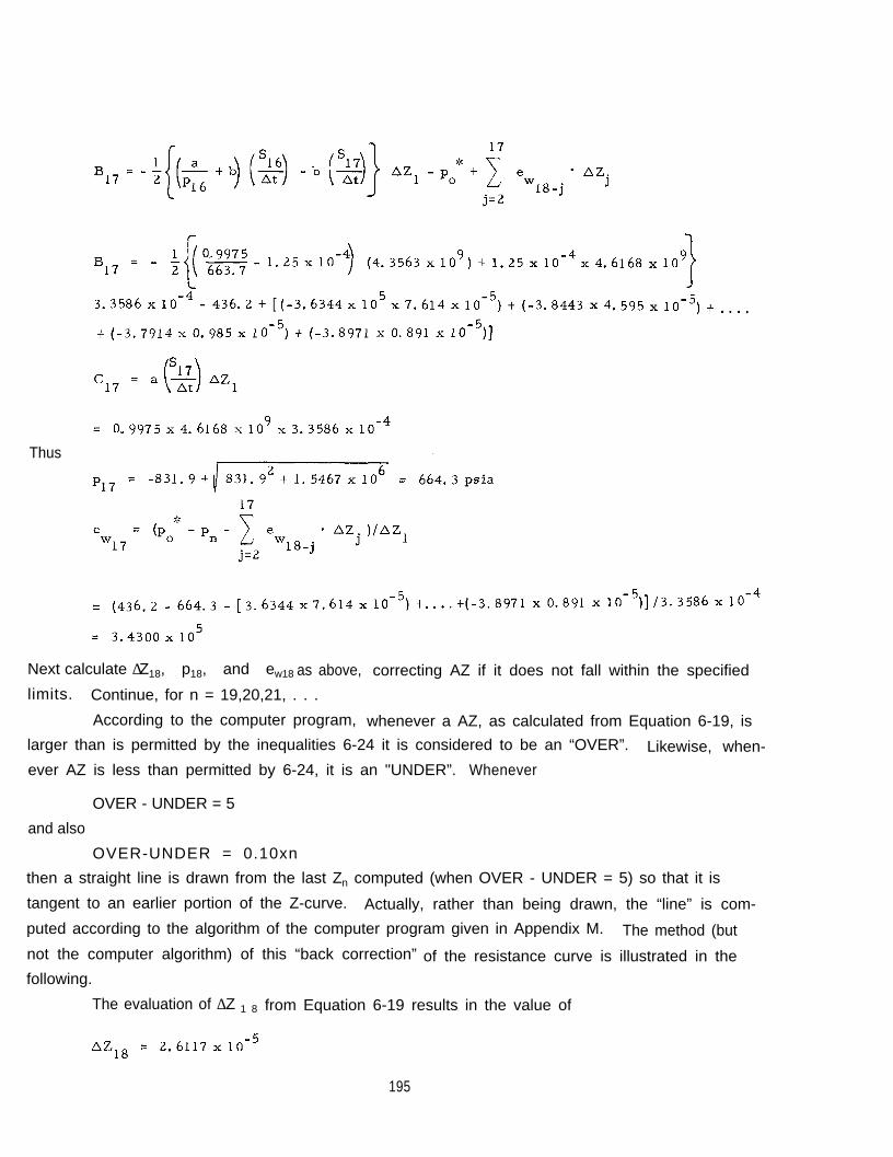
Thus
Next calculate ∆ Z18, p18, and ew18 as above, correcting AZ if it does not fall within the specifiedlimits. Continue, for n = 19,20,21, . . .
According to the computer program, whenever a AZ, as calculated from Equation 6-19, islarger than is permitted by the inequalities 6-24 it is considered to be an “OVER”. Likewise, when-ever AZ is less than permitted by 6-24, it is an "UNDER”. Whenever
OVER - UNDER = 5
and also
OVER-UNDER = 0.10xn
then a straight line is drawn from the last Zn computed (when OVER - UNDER = 5) so that it is
tangent to an earlier portion of the Z-curve. Actually, rather than being drawn, the “line” is com-
puted according to the algorithm of the computer program given in Appendix M. The method (butnot the computer algorithm) of this “back correction” of the resistance curve is illustrated in thefollowing.
The evaluation of ∆ Z 1 8 from Equation 6-19 results in the value of
195
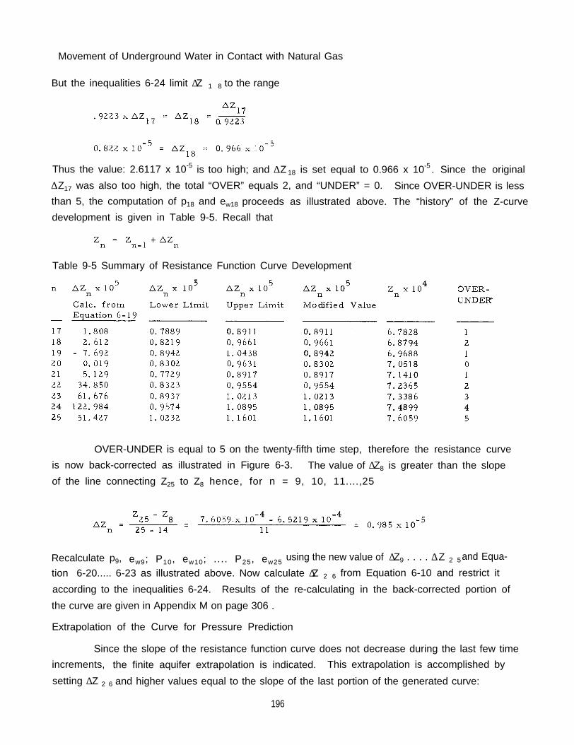
Movement of Underground Water in Contact with Natural Gas
But the inequalities 6-24 limit ∆ Z 1 8 to the range
Thus the value: 2.6117 x 10⁻⁵ is too high; and ∆ Z 18 is set equal to 0.966 x 10⁻⁵ . Since the original
∆ Z17 was also too high, the total “OVER” equals 2, and “UNDER” = 0. Since OVER-UNDER is less
than 5, the computation of p18 and ew18 proceeds as illustrated above. The “history” of the Z-curve
development is given in Table 9-5. Recall that
Table 9-5 Summary of Resistance Function Curve Development
OVER-UNDER is equal to 5 on the twenty-fifth time step, therefore the resistance curve
is now back-corrected as illustrated in Figure 6-3. The value of ∆ Z8 is greater than the slope
of the line connecting Z25 to Z8 hence, for n = 9, 10, 11....,25
Recalculate p9, ew9; P10, ew10; .... P25, ew25 using the new value of ∆ Z9 . . . . ∆ Z 2 5and Equa-
tion 6-20..... 6-23 as illustrated above. Now calculate ∆ Z 2 6 from Equation 6-10 and restrict it
according to the inequalities 6-24. Results of the re-calculating in the back-corrected portion of
the curve are given in Appendix M on page 306 .
Extrapolation of the Curve for Pressure Prediction
Since the slope of the resistance function curve does not decrease during the last few time
increments, the finite aquifer extrapolation is indicated. This extrapolation is accomplished by
setting ∆ Z 2 6 and higher values equal to the slope of the last portion of the generated curve:
196

In order to predict pressures, it is necessary to assume a gas production-injection schedule. In
this case the twenty-seventh through fiftieth gas injection quantities are used and corres-ponding reservoir pressures are calculated to compare with the observed values. Should one wish
to predict the future, postulated gas injection and withdrawal quantities are used to find correspond-
ing reservoir pressures.
Conclusions
Application of all flow models and the resistance function to Field A resulted in good agree-
ment between observed and calculated pressures for its entire history (Figures 9-5, 9-8, 9-10,
9-12, and 9-16). Volume ratios calculated from the predicted pressures are shown in Figures
9-6, 9-9, 9-11 and 9-13. It can be shown that the percentage error is necessarily the same for
a volume ratio prediction as for the corresponding pressure prediction. The radial model gave
the best prediction of all the flow models, although acceptable predictions are obtained using the
other flow models. The resistance function method gave a very good prediction as well.
The straight line exhibited by the latter portion of the resistance curve (Figure 9-15)
indicates that the aquifer’s outer boundary is influencing the field’s pressure behavior; i. e., that
the aquifer is finite. This observation was confirmed with the radial model when a better pressure
prediction was obtained with a finite reservoir, R = 14, than was obtained with an infinite reservoir.
The optimizing of Vo and Kr or Kp in the model calculations appears to utilize the perform-
ance information so that reliable predictions of pressure generally can be made using geometric
models. The resistance function is an extension of the use of performance data which may be
expected to improve the agreement between computed and observed pressures in some cases. As
will be shown in Chapter 11, the moving boundary case can be handled by the resistance function
method.
197

This Page Intentionally Left Blank
CHAPTER 10
CASE STUDIES - PRODUCTION AND STORAGE IN PRODUCING FIELDS
A case study of a gas storage field was presented in Chapter 9 along with a detailed
illustration of the application of the working equations for predicting the movement of water in
contact with natural gas. The pressure behavior of four additional gas fields will be analyzed in
this chapter. Three are gas storage fields located near large population centers making it possi-
ble to supply gas to consumers during periods of high demand. The remaining field, a high-
pressure gas producing field, is located in a remote area. Gas is injected in the storage fields
during periods of low gas demand enabling the gas pipelines to transmit gas at full load from the
remote areas to the population centers when the demand for natural gas is low.
Field B
Field B, a natural gas storage reservoir, produced gas for eight years prior to conver-
sion to gas storage operation. The reservoir was substantially depleted during the initial eight
years when 3,582,000 MCF were produced accompanied by a wellhead pressure decline from 1900
to 212 pounds per square inch gauge.
Geology and Field Data
This field consists of weak cemented sandstone composed of fairly coarse to medium-
grained quartz, open in texture, with small amounts of secondary silica and calcite as cementing
material. The sandstone was deposited during a rapidly westward advancing sea; the old shore
deposits were reworked during temporary interruptions of this encroachment. When present, the
sandstone is generally found to be a sheet spreading over wide areas.
The structure is a small dome, elongated east and west, and bracketed by two parallel
reverse faults to the north and south. These faults suggest that the linear model would best
approximate this reservoir. An areal sketch of the gas and water boundary is shown in Figure
10-1.
The reservoir and fluid properties are summarized in Table 10-1 and the production-
pressure history given in Table 10-2. The pressure data are the weighted average of several
observation wells.
Nearly all the virgin gas was produced prior to the date of storage conversion. This
quantity of gas, converted to the initial reservoir temperature and pressure, was used as a lower
limit for estimating the initial pore volume. This limit (Vo = 23.8 million cubic feet) was closeto the value which gave the minimum deviation between calculated and observed pressures, 24.0
million cubic feet of reservoir pore space.
199
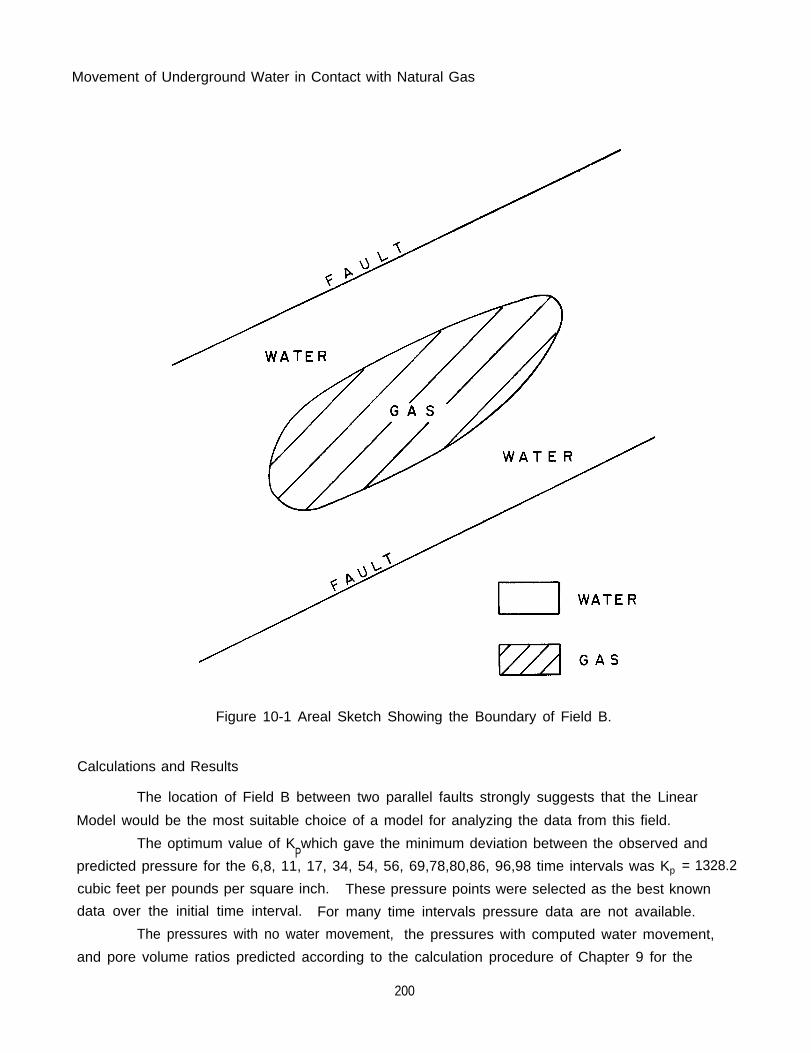
Movement of Underground Water in Contact with Natural Gas
Figure 10-1 Areal Sketch Showing the Boundary of Field B.
Calculations and Results
The location of Field B between two parallel faults strongly suggests that the Linear
Model would be the most suitable choice of a model for analyzing the data from this field.
The optimum value of K which gave the minimum deviation between the observed andP
predicted pressure for the 6,8, 11, 17, 34, 54, 56, 69,78,80,86, 96,98 time intervals was Kp = 1328.2
cubic feet per pounds per square inch. These pressure points were selected as the best known
data over the initial time interval. For many time intervals pressure data are not available.
The pressures with no water movement, the pressures with computed water movement,
and pore volume ratios predicted according to the calculation procedure of Chapter 9 for the
200

Table 10-1 Storage Field B Reservoir Data
201

Movement of Underground Water in Contact with Natural Gas
Table 10-2 Gas Inventory and Pressure History for Field B
Pressure Base 14.73 psiaTemperature Base = 60°F
202

Table 10-2 (continued)
203
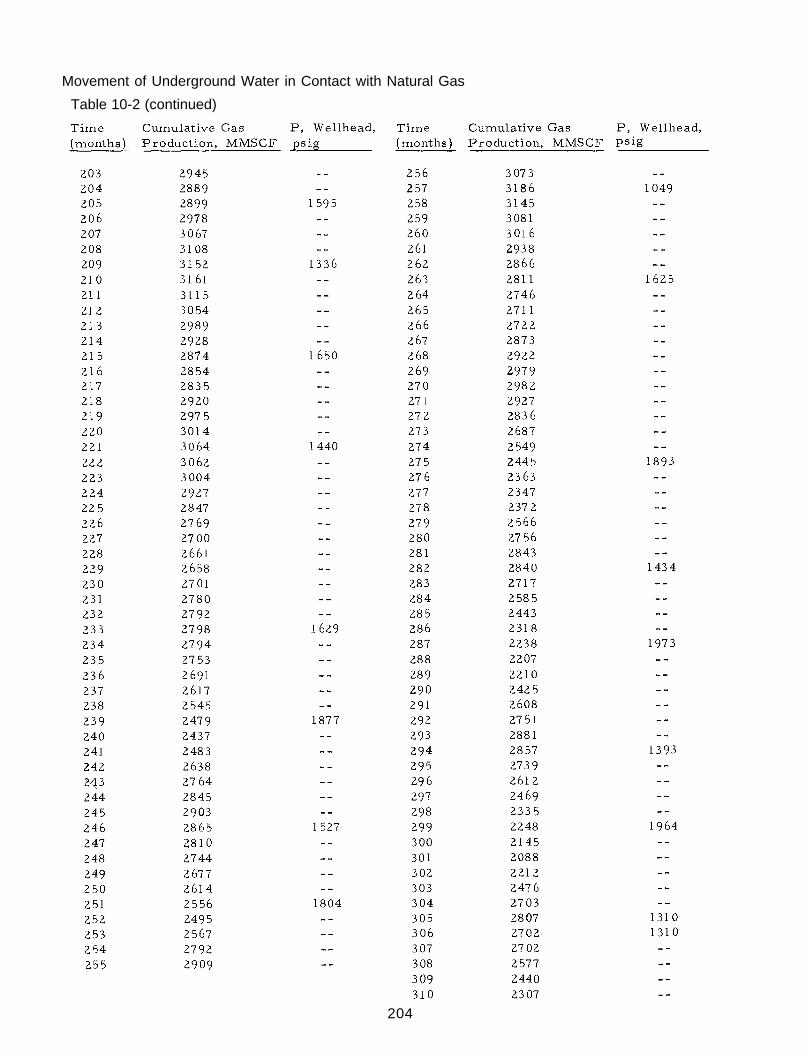
Movement of Underground Water in Contact with Natural Gas
Table 10-2 (continued)
204

Linear Model are shown in Figures 10-2, 10-3 and 10-4.
In order to test the effect of errors in the initial gas production data, the gas production
schedule for the initial 98 time intervals was changed to a hypothetical production schedule with
a steady decline curve. The 127, 128, 133, 136, 141, 147, 149, 151, 152, 153, 154, 162, 180
time intervals were used instead of the initial data to optimize the value of Kp . The pressure
prediction, shown in Figure 10-5 is in good agreement with Figure 10-3 for the later history of
the field. Since the initial gas production history of the field is different for the hypothetical
study, the observed pressure does not agree with the predicted over this section.
Pressures calculated assuming no water movement are considerably lower than observed
pressures after the initial drawdown (Figure 10-2). Considerable improvement is obtained when
the rate of water movement is determined by use of the linear model (Figure 10-3). A comparison
of the reservoir volume ratios calculated from these pressures is given in Figure 10-4. Note
that at one time during the history of the field about 85 per cent of the volume originally occupied
by the gas has been replaced by water, thus the gas bubble prior to gas injection occupied only
15 per cent of the initial pore volume.
Field C
Field C was produced six years prior to conversion to gas-storage operation. During
this period, 8, 026, 657 MCF of gas were produced accompanied by a pressure decline from 453
pounds per square inch to 267 pounds per square inch (wellhead). Recovery of pressure after
short periods of high production indicated the gas-water interface was mobile.
Geology and Field Data
Field C is one of several gas reservoirs found in Michigan stray sand. This sand is a
series of disconnected lenses located at random rather than a continuous layer of sandstone.
For this reason, the formation has been designated as stray sand. The sand was deposited dur-
ing the geologic time known as the “Michigan” and is an integral part of the Michigan formation.
Underlying the stray sand is the Marshall formation, a porous and permeable sandstone
like the stray. Although several shale lenses are found between the stray and Marshall forma-
tions, no consistent thickness of sealing shale is found between the two structures. In many
places water in the Marshall is free to migrate into the stray if the pressure within the stray
is reduced.
The invasion of the Marshall water into the stray helps maintain the pressure in the stray.
Providing that the movement of this water is controlled and is not allowed to come into a produc-
tion well, thereby waterlogging the well, the water is beneficial.
A summary of reservoir and fluid properties is given in Table 10-3 and the production-
pressure history is tabulated in Table 10-4. The pressures are the weighted average of several
observation wells.
205

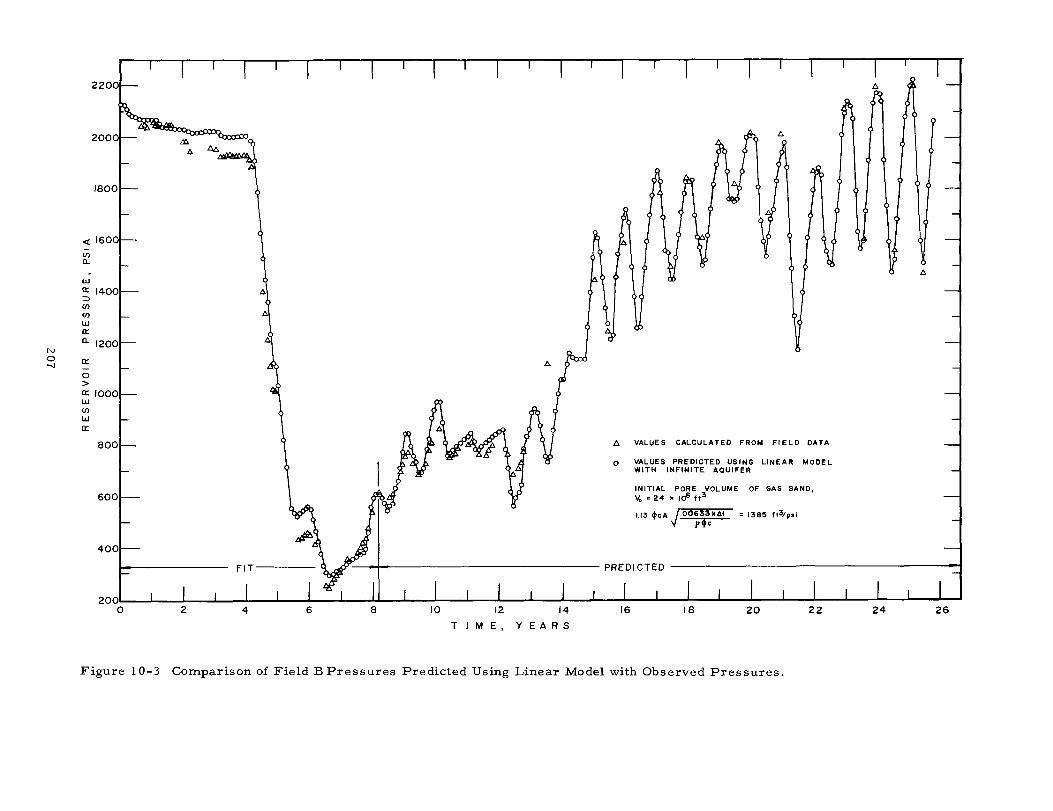


Movement of Underground Water in Contact with Natural Gas
Table 10-3 Storage Field C Reservoir Data
210

Table 10-4 Gas Inventory and Pressure History for Field C
211

Movement of Underground Water in Contact with Natural Gas
Table 10-4 (continued)
212

Table 10-4 (continued)
213

Movement of Underground Water in Contact with Natural Gas
Figure 10-6 Areal Sketch Showing Boundary of Gas Field C.
Calculations and Results
The available geological information on Field C suggests the radial model would be the
best flow model. The optimum values of the coefficients for the flow model were obtained by
minimizing the differences between observed and predicted pressures for the 5, 8, 11, 16, 19,
23, 26, 30, 33, 37, 40, 42, 49, 52, 54, 57, 60, 63, 66 time intervals. These time intervals
are believed to be the most accurate pressure measurements. The best agreement between ob-
served and predicted pressures was obtained for a finite aquifer, R = 6 with Kp = 30, 200. Pre-
dicted pressures and pore volume ratios are shown in Figures 10-8 and 10-9, respectively.
Predicted pressures assuming no water movement are compared with the observed field
214


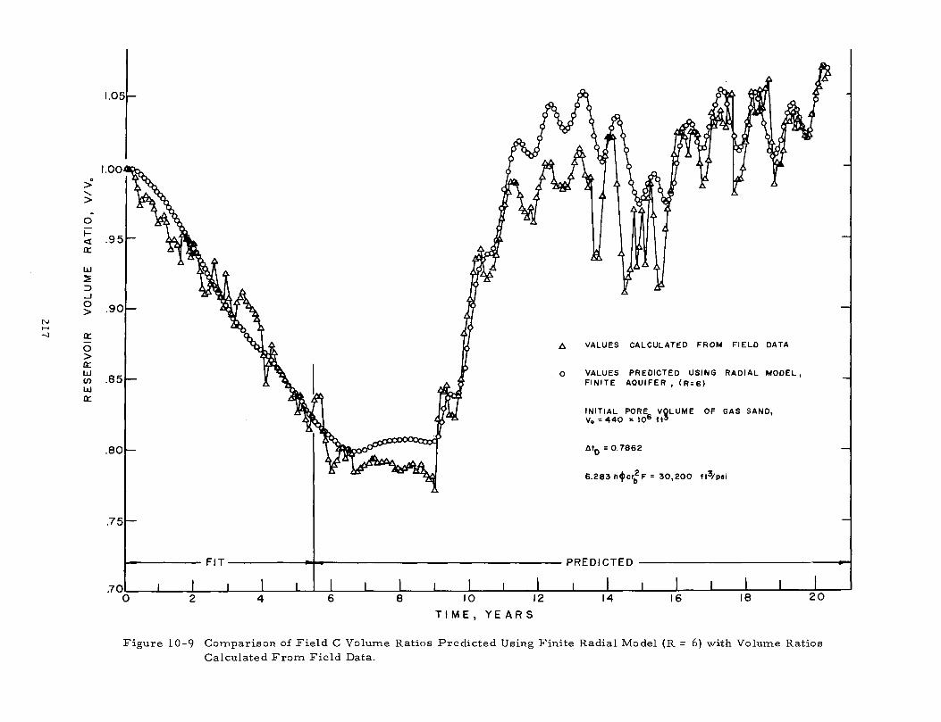
Movement of Underground Water in Contact with Natural Gas
pressure history in Figure 10-7. The deviation between these two curves is considerable during
the first ten years’ operation, but decreases after gas storage begins. This improvement may
be attributed in part to the cycling of the pressures about the discovery pressure.
The pressures predicted using the radial model with an infinite aquifer were high during
the latter portion of the field history indicating that the aquifer is of finite rather than of infinite
extent. Therefore, the finite radial model with several values of R, the ratio of the aquifer radius
to the gas bubble radius was tried. Good agreement for the entire history was obtained for R = 6.
This is shown in Figure 10-8.
The variation with time of the reservoir volume ratio, V/V0 (the present gas bubble
volume divided by the initial gas volume), calculated from field data and also the radial model
(R = 6), is shown in Figure 10-9.
Unfortunately, little attention was paid to aquifer viscosity during this study.
Actually, the Marshall brine has a density of 1.22 grams per milliliter and has a viscosity some
1.5 times that used in the calculations. It seems unlikely that the performance of the aquifer as
limited when it is continuous in extent for miles could be due to the use of the low viscosity in the
calculations.
Field D
Field D, a large gas field in the Michigan Basin, had an original void space of 900 million
cubic feet and discovery pressure of 1346 pounds per square inch absolute (well bottom), To date,
111 storage wells and 23 observation wells have been drilled. Before the field was converted to
storage operation, more than 16 billion standard cubic feet had been produced.
An areal sketch of this field is shown in Figure 10-10.
Geology and Field Data
In contrast to the previous fields investigated, the composition of the gas horizon in Field
D is dolomite instead of sandstone. This dolomite is very “tight” with an estimated permeability
of only 2.4 millidarcys. This formation is designated as the A2 dolomite in the Salina Formation
of the Silurian Age.
The gas and aquifer properties are summarized in Table 10-5 and the gas inventory
and pressure history is listed in Table 10-6.
The value for the initial pore volume which gave the best agreement between observed
and predicted pressures for both the radial model and resistence function method was 900 million
cubic feet.
Calculations and Results
A comparison of the observed and predicted pressures (Figure 10-11) with the assump-
tion of no water movement in the radial gas bubble, shows the predicted pressures arenot in agreement with those observed. Part of the disagreement can be rationalized when one
218

Table 10-5 Storage Field D Data
219
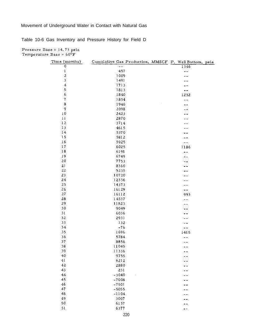
Movement of Underground Water in Contact with Natural Gas
Table 10-6 Gas Inventory and Pressure History for Field D
220

Figure 10-10 Areal Sketch Showing Boundary of Field D.
considers the pressure gradients within the gas bubble itself. In the previous fields investigated,
the permeability of the gas formation is several orders of magnitude larger, thereby allowing use
of an average gas pressure for the entire field. As a result of the low permeability in this field,
pressure gradients of several hundred pounds within the gas bubble itself have been observed.
When these gradients are considered, the discrepancy between observed and predicted pressure
is not surprising.
The calculations of pore volurne ratios (Figure 10-13) show only a slight water movement
is present, the void space being reduced by less than 5 per cent prior to gas injection.
221


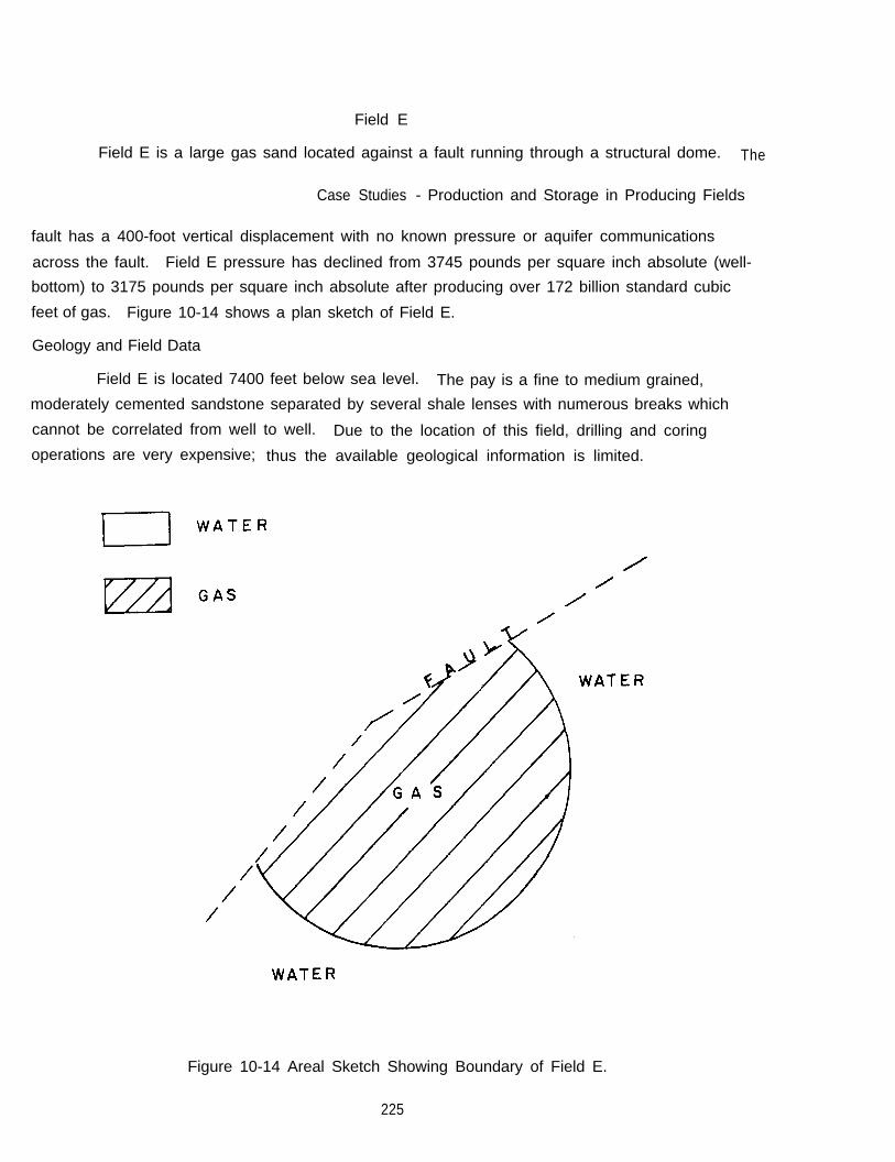
Field E
Field E is a large gas sand located against a fault running through a structural dome. The
Case Studies - Production and Storage in Producing Fields
fault has a 400-foot vertical displacement with no known pressure or aquifer communications
across the fault. Field E pressure has declined from 3745 pounds per square inch absolute (well-
bottom) to 3175 pounds per square inch absolute after producing over 172 billion standard cubic
feet of gas. Figure 10-14 shows a plan sketch of Field E.
Geology and Field Data
Field E is located 7400 feet below sea level. The pay is a fine to medium grained,
moderately cemented sandstone separated by several shale lenses with numerous breaks which
cannot be correlated from well to well. Due to the location of this field, drilling and coring
operations are very expensive; thus the available geological information is limited.
Figure 10-14 Areal Sketch Showing Boundary of Field E.
225
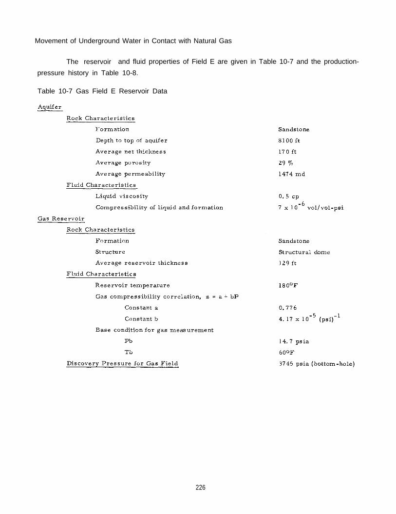
Movement of Underground Water in Contact with Natural Gas
The reservoir and fluid properties of Field E are given in Table 10-7 and the production-
pressure history in Table 10-8.
Table 10-7 Gas Field E Reservoir Data
226
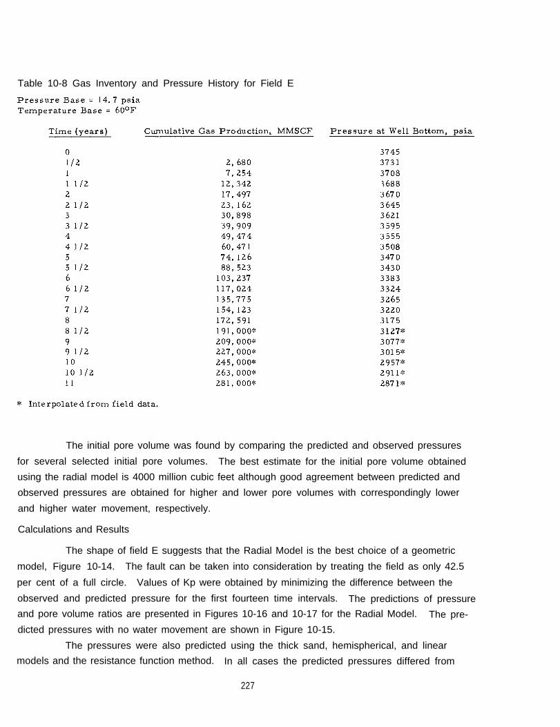
Table 10-8 Gas Inventory and Pressure History for Field E
The initial pore volume was found by comparing the predicted and observed pressures
for several selected initial pore volumes. The best estimate for the initial pore volume obtained
using the radial model is 4000 million cubic feet although good agreement between predicted and
observed pressures are obtained for higher and lower pore volumes with correspondingly lower
and higher water movement, respectively.
Calculations and Results
The shape of field E suggests that the Radial Model is the best choice of a geometric
model, Figure 10-14. The fault can be taken into consideration by treating the field as only 42.5
per cent of a full circle. Values of Kp were obtained by minimizing the difference between the
observed and predicted pressure for the first fourteen time intervals. The predictions of pressureand pore volume ratios are presented in Figures 10-16 and 10-17 for the Radial Model. The pre-
dicted pressures with no water movement are shown in Figure 10-15.
The pressures were also predicted using the thick sand, hemispherical, and linear
models and the resistance function method. In all cases the predicted pressures differed from
227
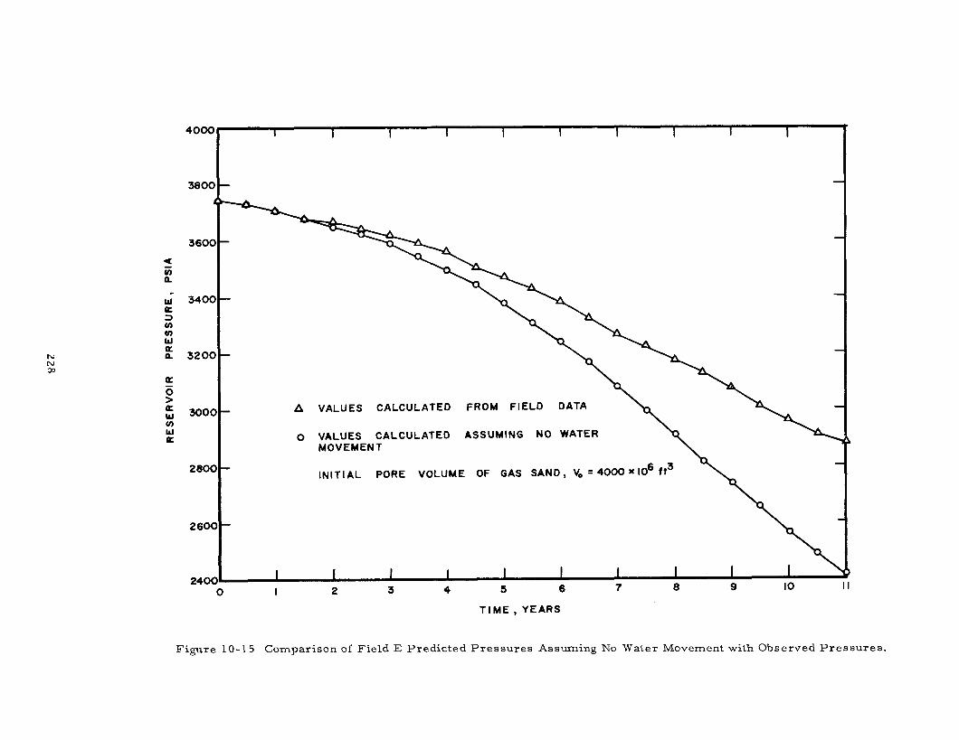


the observed pressure by less than one per cent. Since all flow models gave good agreement
between the observed and predicted pressures, additional data would be necessary to ascertain
the correct flow model. Any of the above models can be used to predict the reservoir pressures
until a sufficient number of time steps are available causing the deviation between observed and
predicted pressures to become significant.
Application of the radial model, the closest approximation of the reservoir shape
(Figure 10-14), with an infinite aquifer to the field data gave a predicted performance almost
identical to that observed (Figure 10-16). This agreement is also reflected in the volume ratios
calculated from these pressures (Figure 10-17). As all the predicted pressures are in good
agreement with the observed, the effect of the boundary of the aquifer has not had time to influ-
ence the pressure history.
It was found that a plot of Vo versus minimum deviation between observed and computed
pressures was a relatively flat curve. It is believed that steady gas production without giving any
independence to gas volumes and water movement may be the cause for the flatness. The reversalin water movement by gas injection normally assists in giving a sharp minimum value for Vo.
231

This Page Intentionally Left Blank
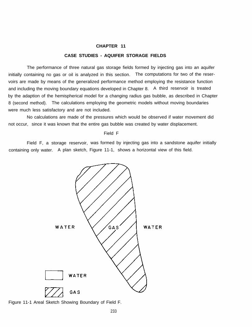
CHAPTER 11
CASE STUDIES - AQUIFER STORAGE FIELDS
The performance of three natural gas storage fields formed by injecting gas into an aquifer
initially containing no gas or oil is analyzed in this section. The computations for two of the reser-
voirs are made by means of the generalized performance method employing the resistance function
and including the moving boundary equations developed in Chapter 8. A third reservoir is treated
by the adaption of the hemispherical model for a changing radius gas bubble, as described in Chapter
8 (second method). The calculations employing the geometric models without moving boundaries
were much less satisfactory and are not included.
No calculations are made of the pressures which would be observed if water movement did
not occur, since it was known that the entire gas bubble was created by water displacement.
Field F
Field F, a storage reservoir, was formed by injecting gas into a sandstone aquifer initially
containing only water. A plan sketch, Figure 11-1, shows a horizontal view of this field.
Figure 11-1 Areal Sketch Showing Boundary of Field F.
233

Movement of Underground Water in Contact with Natural Gas
Geology and Field Data
The storage sand,
feet thick. This sand consi
encountered at an average depth of 2450 feet below the surface, is 2500
sts of alternate layers of fine- to very-coarse-grained sandstone with
several randomly spaced, non-continuous, thin, green shale laminations. The thin laminations
at intervals presents full vertical pressure penetration.
Impervious layers of dolomite and shale form the cap rock. The lower two layers of
dolomite and shale in this cap rock are more than twenty and forty feet thick, respectively.
No faults are known to exist in the immediate vicinity of the aquifer.
information indicates the aquifer is infinite.
A summary of the reservoir and aquifer properties is given in Table
pressure history is tabulated in Table 11-2.
Table 11-1 Storage Field Reservoir Data
Available geological
11-1 and the production-
234

Table 11-2 Gas Inventcry and Pressure History for Field F
235

Movement of Underground Water in Contact with Natural Gas
Table 11-2 (cont'd)
236

Calculations and Results
Since the sand containing gas and water was thick, and the gas-water interface moves
rather drastically in early stages, the hemispherical model as modified was employed. The first
fourteen points (weeks) were not used, but rather 15 through 60 were selected in comparing calcu-
lated and observed pressures to determine the coefficient to be used in predicting future performance.
The coefficient was then used to predict behavior from 61 weeks through 171 weeks. Figure 11-2shows the results of the reservoir pressures computed as compared to the observed values. The
shapes of the curves are somewhat different, possibly reflecting the layered nature of the sand and
lack of vertical pressure penetration.
Various values of α in Equation 8-24 were tried in the solution. The value of α = 0.50
which corresponds to a parabolic cap rock geometry used for the results in Figure 11-2.
The resistance function method was tried and it gave the proper shape of the pressure
curve. However, the amplitude of the cyclic pressure variation was much smaller than the observed
values , indicating the actual resistance exceeded that predicted from early behavior.
Field G
Field G, on the fringe of the Illinois basin, is an aquifer type-gas storage field. An areal
view of Field G is shown in Figure 11-3 and cross sectional views are given in Figures 11-4 and
11-5.
Geology and Field Data
Field G utilizes the Eau Claire and Mt. Simon formations in the St. Croixau Series in the
Illinois basin. The structure is an asymmetrical east -west trending anticline with 120 feet ofCambrian closure. The cap rock over these formations consists of dense shales and argillaceous
dolomites.
The 245 foot thick, lower unit of the Eau Claire consists of three fine to coarse grained
porous sandstones separated by dense, dark green dolomitic shales and argillaceous nodular dolo-
mite. The lower two sands are usable storage sands. Several faults along the northern edge of
the reservoir allow the gas to migrate between these sands and the underlying Mt. Simon, Gas isinjected into the Mt. Simon and B sands and produced from all four zones. The sand to sand faces
at the faults give good communication while the shale to shale contacts at the fault hold gas satis-
factorily. Figures 9-3, 9-4 and 9-5 show the areal extent of the field and two sections.
The thickness of the Mt. Simon sandstone is 2112 feet and consists of siltstone, very fine
grained to granular sandstone and scattered thin red and green sandy shales.
The Mt. Simon’s pressures will be used and predicted in this study and the gas injection
quantities are the sum of the Mt. Simon and the B zone injections.
The reservoir and properties of Field G are given in Table 11-3 and the production-
pressure history in Table 11-4.
237

Figure 11-2 Comparison of Predicted and Observed Pressures for Field F.
238

Figure 11-3 Areal View of Field G.
239
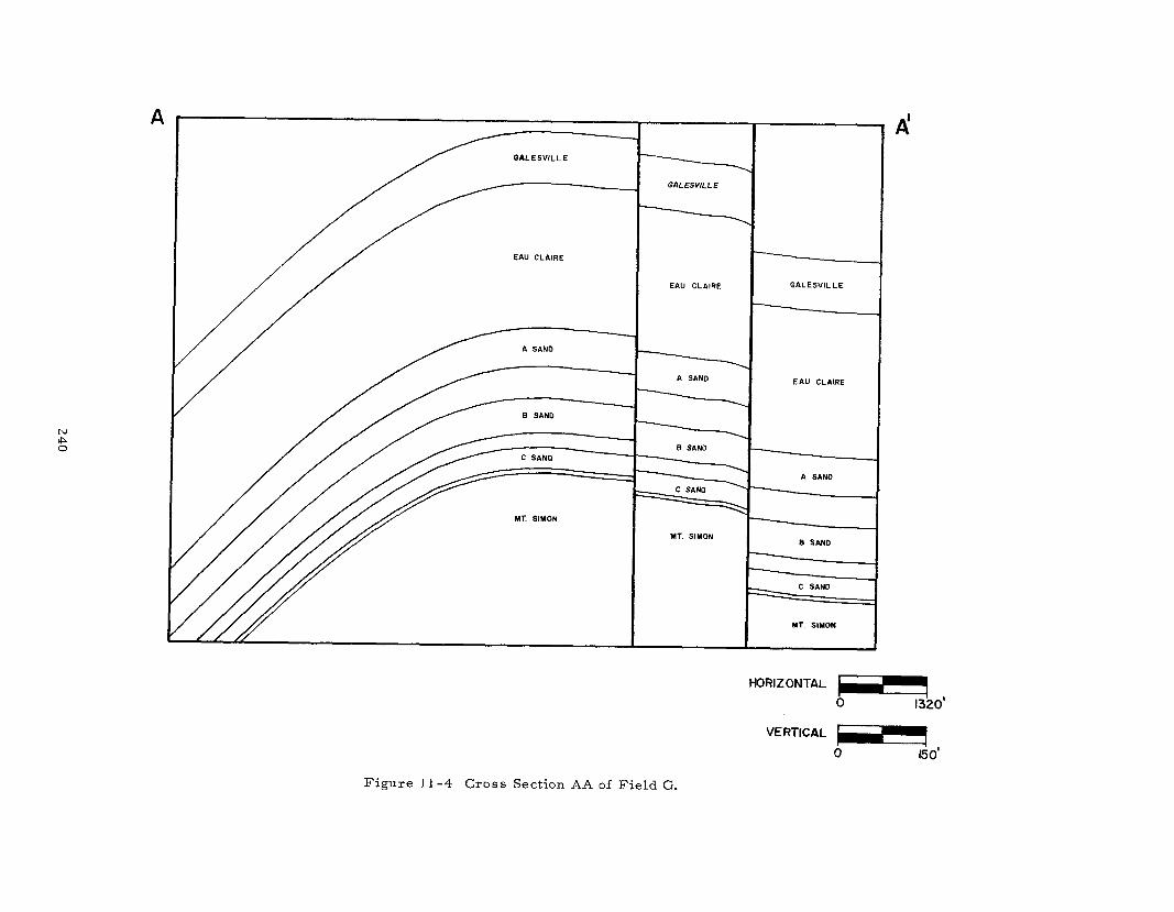

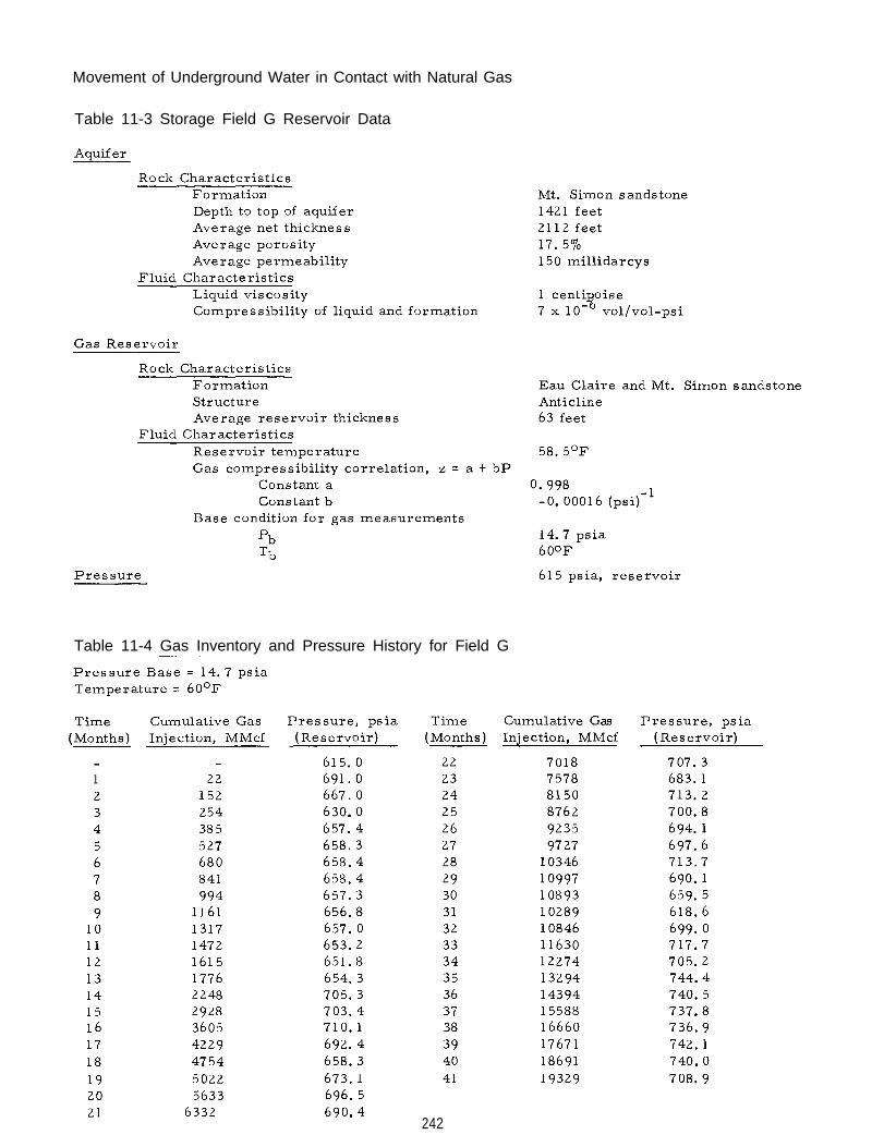
Movement of Underground Water in Contact with Natural Gas
Table 11-3 Storage Field G Reservoir Data
Table 11-4 Gas Inventory and Pressure History for Field G
242

Calculations and Results
The resistance function method was used, as modified for the moving boundary of Chapter
8 (first method). The radial model was used for the first 16 points (months) and the next 6 points
determined resistance function directly. A linear extrapolation which corresponds to the limited
aquifer was employed, as shown on Figure 11-6.
Figure 11-6 Resistance Function for Field G.
243

Figure 11-7 Comparison on Predicted and Observed Pressures for Field G.
244

Various values of α for the moving boundary modification were tried including 0.7, 1.0,
1.5, and 2.0. The best results were found for 2.0; the comparison of computed and observed
pressures is given on Figure 11-7.
The value of V* was arbitrarily chosen as one-half the maximum gas bubble volume or
176.8 x 10⁶ cubic feet.
Field H
Gas injection was started into this aquifer-type storage field some five years ago and
withdrawal has occurred during five seasons. A sketch of Field H is shown in Figure 11-8.
Geology and Field Data
Field H is located in the extreme northeastern portion of the Forest City Basin. The
gas storage anticline trends in a north-south direction, is asymmetrical (being steeper on the
east than on the west), and is doubly plunging.
The reservoir, situated in the Mt. Simon sandstone, is composed of sandstone and con-
glomerate. The sandstone ranges from fine to very coarse in size (quartz grains vary from 1/8
to 2 mm. in diameter); the conglomerate ranges from granule (individual quartz grains 2 to 4 mm.
in diameter) to pebble (greater than 4 mm. in diameter) in size. Many shale partings and shaly
sandstone streaks occur in all parts of the Mt. Simon. The individual quartz grains vary in degree
of rounding from subangular to well-rounded. The average thickness of the Mt. Simon reservoir
is 115 feet, the weighted average porosity is 15.8%, and the weighted average permeability is 314
millidarcys.
The cap rock for the Mt. Simon reservoir is the Eau Claire member of the Bresbach
formation which lies immediately above the Mt. Simon reservoir. The Eau Claire is composed
of shaly limestone, limestone and dolomite, shale, siltstone and silty limestone. The Eau Claire
averages in excess of 200 feet in thickness; permeability ranges from less than one-tenth of a
millidarcy to 1 x 10⁻⁶ millidarcys .
The reservoir and aquifer properties are given in Table 11-5 and the production-pressure
history tabulated in Table 11-6.
Calculations and Results
The generalized performance method was employed, with a moving boundary modification
as in Field G. Here α was used as 0.40. For the radial model, 16 time increments (months) were
employed followed by 30 months for the resistance function, Figure 11-9. The pressure behavior
for the remaining 44 months computed on the first try was excellent, Figure 11-10.
The reference volume, V*, used was 172 x 106 cubic feet (see Chapter 8) arbitrarily taken
as one-half the maximum gas bubble volume.
The radial model gave better agreement for Field H than for Field G, possibly because
the aquifer was of limited thickness. However, the results were not based on a moving boundary
245

Movement of Underground Water in Contact with Natural Gas
Table 11-5 Storage Field H Reservoir Data
246

Table 11-6 Gas Inventory and Pressure History for Field H
247

Figure 11-8 Areal Sketch of Field H.
and were not as good as Figure 11-10.
Conclusions
For aquifers, no case study was available with good insitu compressibility and permea-
bility to permit prediction of reservoir pressures prior to injection-pressure experience. It
was found that for a sand of 119 feet in thickness, the resistance function method, modified for
moving boundary, gave a very good prediction of pressures for the injection-withdrawal schedule.
The results for the thick aquifers with a degree of lamination were only moderately
satisfactory. Neither the adapted hemispherical model or the resistance function seemed fully
adequate to the relatively early life of these storage reservoirs. However, the results can be of
utility in predicting the gross reservoir behavior for storage operations.
248


APPENDIX A
Table of Dimensionless Pressure, Pt, forInfinite Radial Aquifer, Constant Terminal Rate. Chatas (5)(35)
251

This Page Intentionally Left Blank
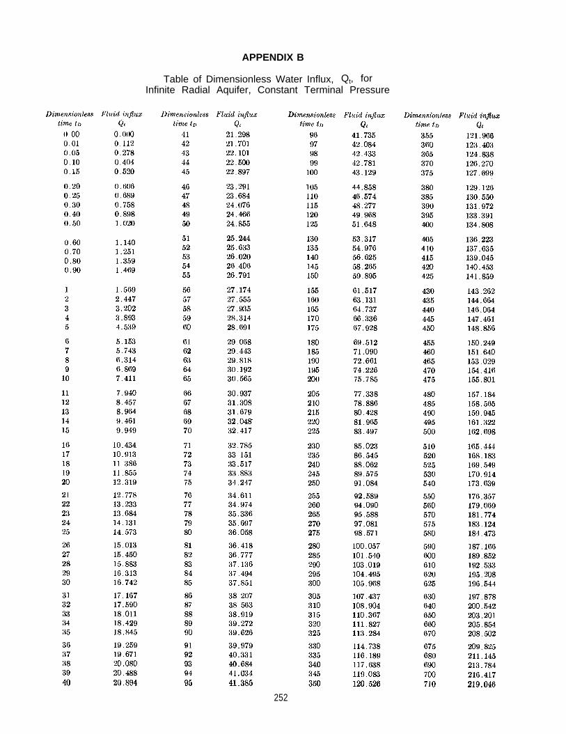
APPENDIX B
Table of Dimensionless Water Influx, Qt, forInfinite Radial Aquifer, Constant Terminal Pressure
252
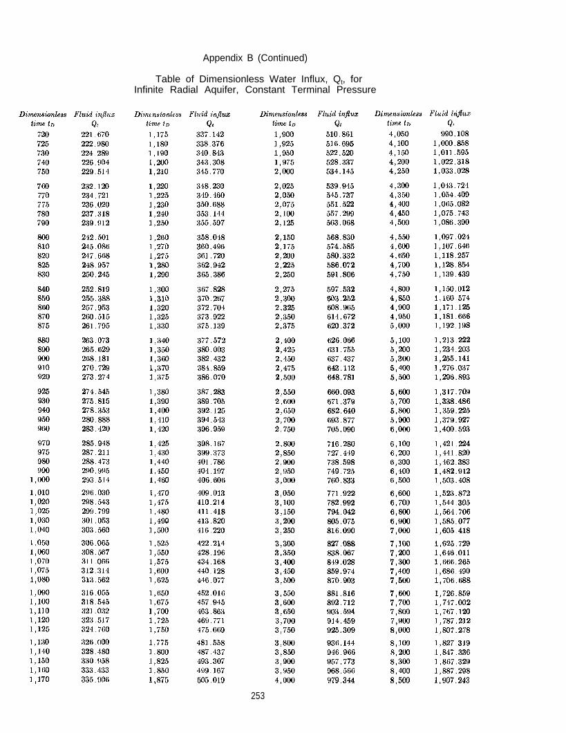
Appendix B (Continued)
Table of Dimensionless Water Influx, Qt, forInfinite Radial Aquifer, Constant Terminal Pressure
253

Appendix B ( Continued)
Table of Dimensionless Water Influx, Qt, forInfinite Radial Aquifer, Constant Terminal Pressure
254

This Page Intentionally Left Blank


This Page Intentionally Left Blank


Appendix D (Continued)
Table of Dimensionless Water Influx, Qt, forFinite Radial Aquifer with Closed Exterior Boundary,
Constant Terminal Pressure. Katz (37)
257
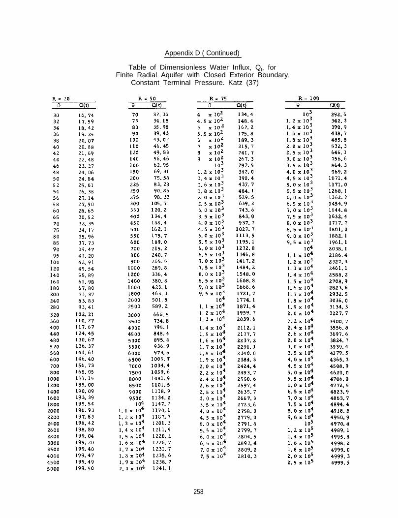
Appendix D ( Continued)
Table of Dimensionless Water Influx, Qt, forFinite Radial Aquifer with Closed Exterior Boundary,
Constant Terminal Pressure. Katz (37)
258

Appendix D (Continued)
Table of Dimensionless Water Influx, Qt, forFinite Radial Aquifer with Closed Exterior Boundary,
Constant Terminal Pressure. Katz (37)
259
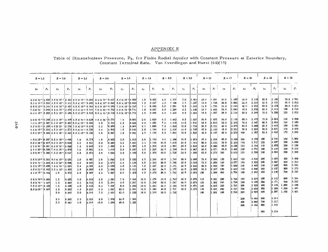

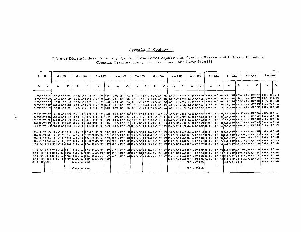

This Page Intentionally Left Blank
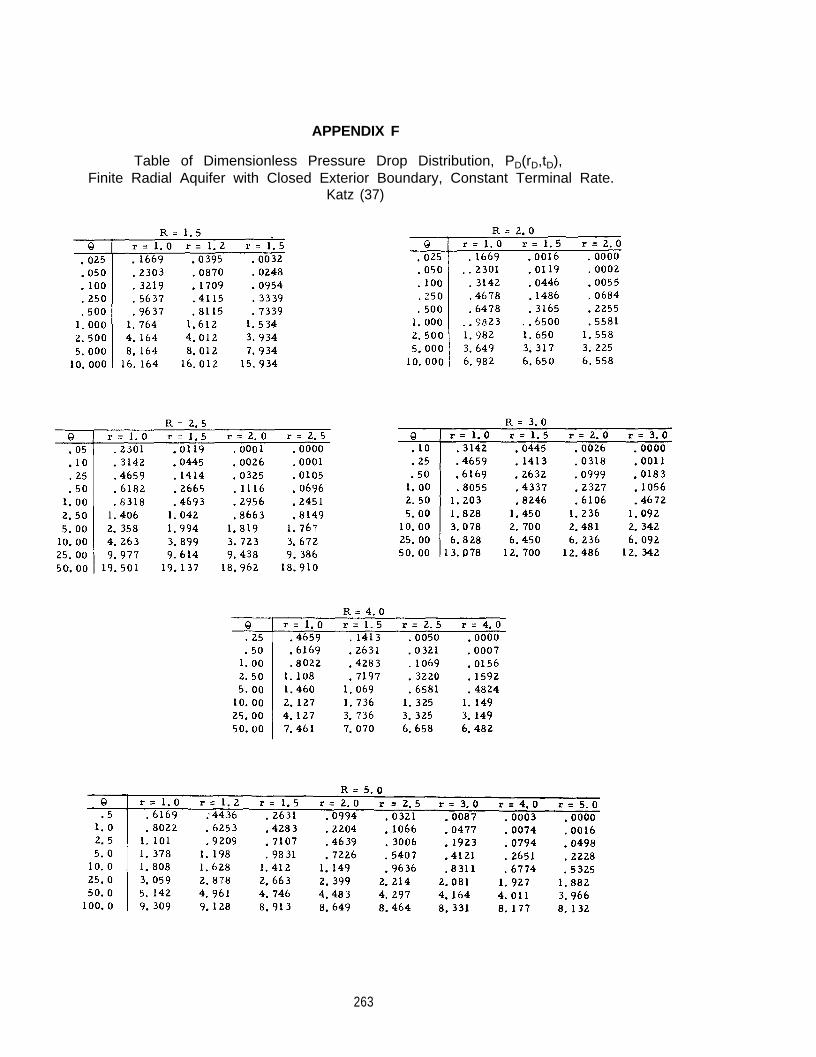
APPENDIX F
Table of Dimensionless Pressure Drop Distribution, PD(rD,tD),Finite Radial Aquifer with Closed Exterior Boundary, Constant Terminal Rate.
Katz (37)
263

Appendix F (Continued)
Table of Dimensionless Pressure Drop Distribution, PD(rD,tD),Finite Radial Aquifer with Closed Exterior Boundary, Constant Terminal Rate.
Katz (37)
264

APPENDIX G
Table of Dimensionless Pressure Drop Distribution, PD( rD , t D ) ,Finite Radial Aquifer with Closed Exterior Boundary,
Constant Terminal Pressure. Katz (37)
265

Appendix G [Continued)
Table of Dimensionless Pressure Drop Distribution, PD(rD,tD),Finite Radial Aquifer with Closed Exterior Boundary,
Constant Terminal Pressure, Katz (37)
266

Appendix G ( Continued)
Table of Dimensionless Pressure Drop Distribution, PDFinite Radial Aquifer with Closed Exterior Boundary,
( rD , t D ) ,
Constant Terminal Pressure. Katz (37)
267
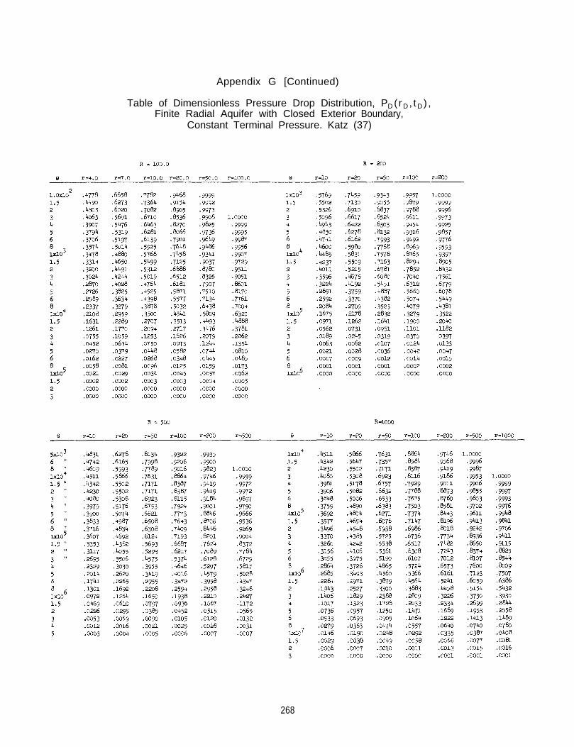
Appendix G [Continued)
Table of Dimensionless Pressure Drop Distribution, PDFinite Radial Aquifer with Closed Exterior Boundary,
( rD , t D ) ,
Constant Terminal Pressure. Katz (37)
268

APPENDIX H
Table of Dimensionless Pressure Distribution, PD(xD,tD),Linear Flow Aquifer with Closed Exterior Boundary,
Constant Terminal Pressure. Katz (37)
269

This Page Intentionally Left Blank
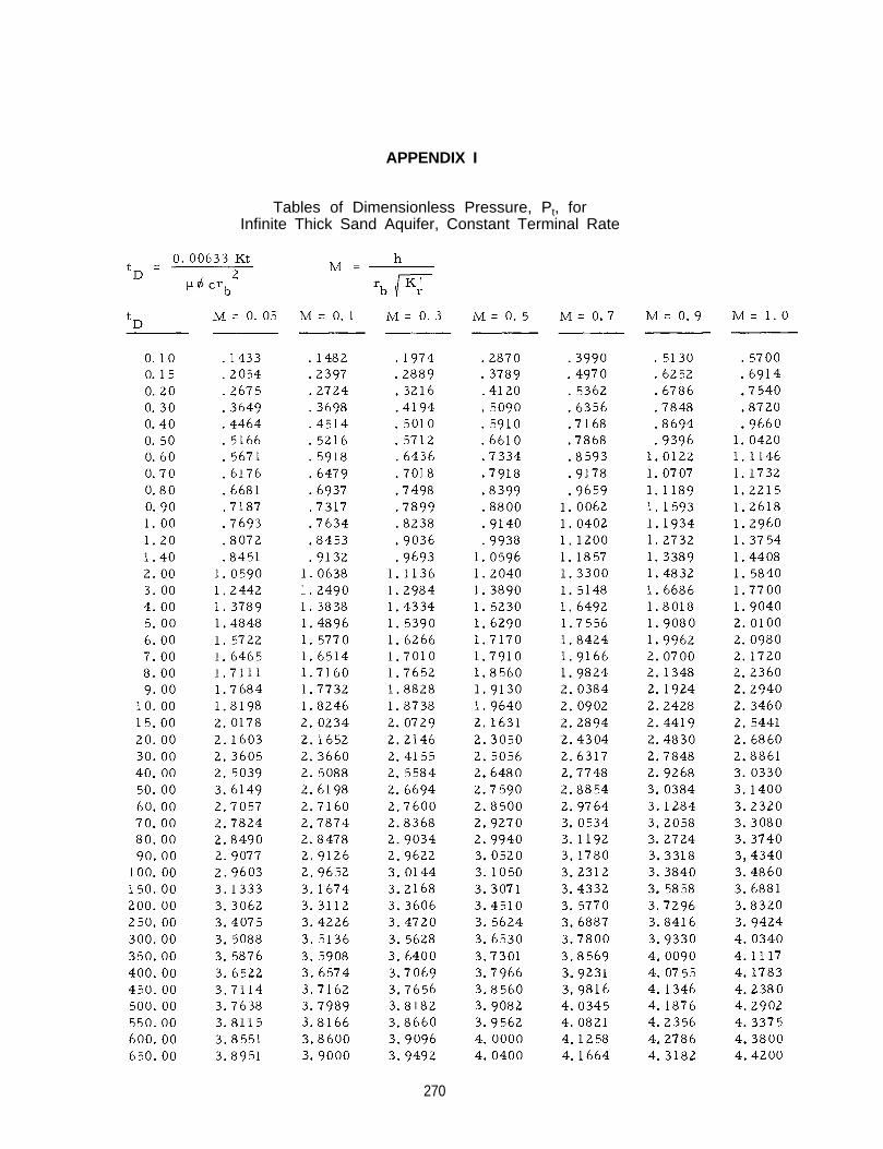
APPENDIX I
Tables of Dimensionless Pressure, Pt, forInfinite Thick Sand Aquifer, Constant Terminal Rate
270

Appendix I (Continued)
Tables of Dimensionless Pressure, Pt, forInfinite Thick Sand Aquifer, Constant Terminal Rate
271
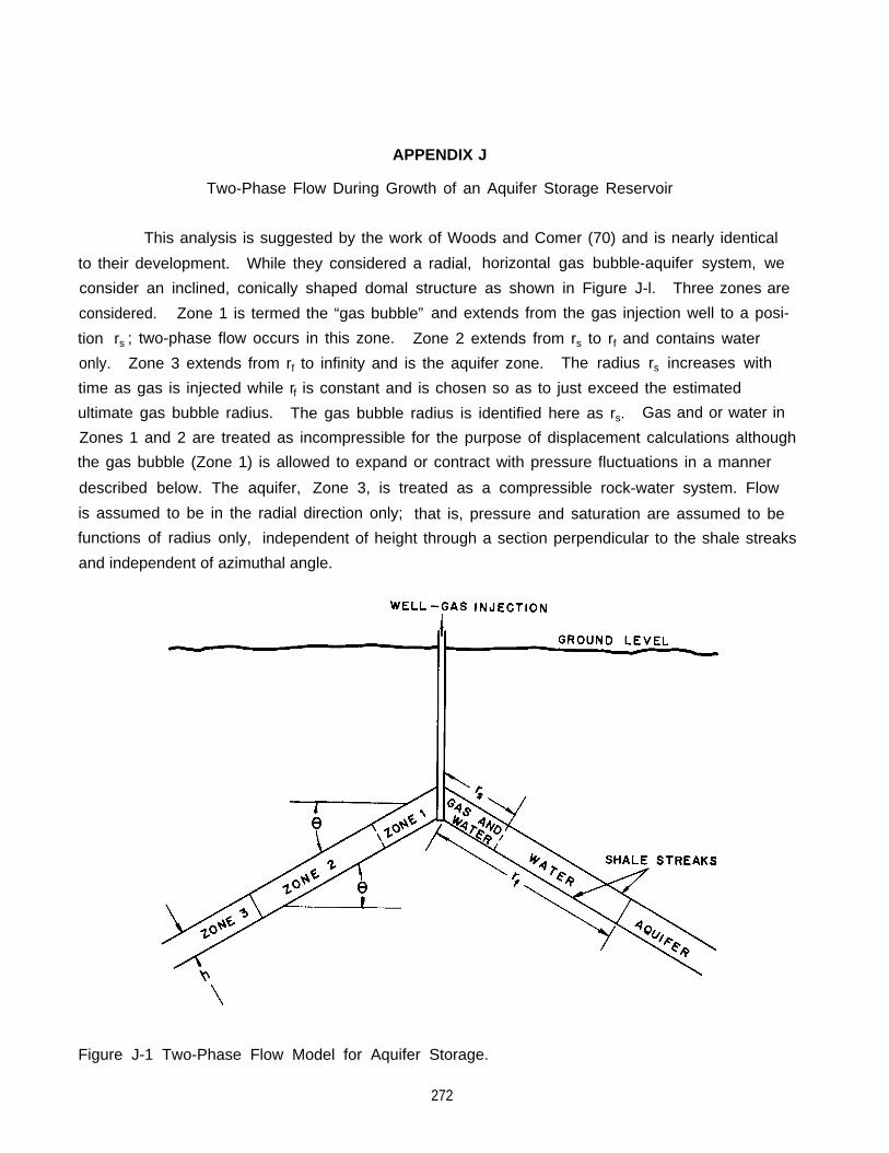
APPENDIX J
Two-Phase Flow During Growth of an Aquifer Storage Reservoir
This analysis is suggested by the work of Woods and Comer (70) and is nearly identical
to their development. While they considered a radial, horizontal gas bubble-aquifer system, we
consider an inclined, conically shaped domal structure as shown in Figure J-l. Three zones are
considered. Zone 1 is termed the “gas bubble” and extends from the gas injection well to a posi-
tion rs ; two-phase flow occurs in this zone. Zone 2 extends from rs to rf and contains water
only. Zone 3 extends from rf to infinity and is the aquifer zone. The radius rs increases with
time as gas is injected while rf is constant and is chosen so as to just exceed the estimated
ultimate gas bubble radius. The gas bubble radius is identified here as rs. Gas and or water in
Zones 1 and 2 are treated as incompressible for the purpose of displacement calculations although
the gas bubble (Zone 1) is allowed to expand or contract with pressure fluctuations in a manner
described below. The aquifer, Zone 3, is treated as a compressible rock-water system. Flow
is assumed to be in the radial direction only; that is, pressure and saturation are assumed to be
functions of radius only, independent of height through a section perpendicular to the shale streaks
and independent of azimuthal angle.
Figure J-1 Two-Phase Flow Model for Aquifer Storage.
272

The radius rs is a function of time and is calculated by solving equations governing the
two-phase flow in Zone 1 (the gas bubble). A material balance, written for gas, about the differen-
tial element of circumference 2- π r lying between r and r + dr gives
(J-1)
where v is the superficial velocity of gas in the r direction and s is gas saturation (fraction of pore
space occupied by gas). The total flow rate across any cylindrical surface of radius r and height
h is
(J-2)
where vT is total fluid velocity (volume of gas and water flowing per unit area normal to flow per
unit time) in the r direction. Since gas and water are treated as incompressible in the flow calcu-
lations, qT must be independent of radius r. Defining fg as the fractional flow of gas, v /v T (whereVW is water flow rate or velocity, volume/(area)(time)), we have
(J-3)
Substituting vT from (J-3) into (J-2) we obtain
Substitution of rv from (J-4) into (J-l) yields
(J-4)
(J-5)
The fractional gas flow fg is a function of gas saturation (s) only, as will be shown below, so that
(J-5) becomes
(J-6)
where fg' = dfg(s)/ds. Since ds(r,t) = we have, at constant s,
Insertion of 2s/ t/ s/ r from (J-6) into (J-7) gives
(J-7)
(J-8)
which gives the rate of advance, dr/dt, of the saturation s, at which fg‘(s) is evaluated. Integrationof (J-8) between r = rW at t = 0 and r, t yields
273

(J-9)
The position rs is determined from (J-9) by using the fg ’ value corresponding to the frontal satura-
tion sf. This saturation sf is easily determined by the tangent construction method of Welge (67a).
The method involves determination of that point (ss,f ) for which f /s = fg'(ss). Thus
The value of ss may be of the order of 0.10 (70).
The expression for fg when gravity is included is (67a)
(J-10)
where
m
k Wk g
µW
µ g
mobility ratio = (kw/pw)/(kg/µg)
relative permeability to water, a function of s
relative permeability to gas, a function of s
water viscosity
gas viscosity
dip angle of formation (see Figure J-l )
∆ P
pW
pg
pw - Pgwater density
gas density
(J-11)
The pressure at the “aquifer radius” rf is equal to the injection pressure p minus theWpressure drop due to gravity and flow in the zones 1 and 2. Since the gas flow rate in these zones
is
the pressure difference pw - pf is (upon integration)
This integration can be performed if saturation s is known as a function of r since fg and kg are
single-valued functions of s.
The one remaining equation needed is that relating pressure pf at the “aquifer inner
boundary” fr to water movement into the aquifer at rf,
274

(J-l 4)
Superposition is necessary because the pressure pf will vary with time.
Equations (J-9), (J-11), (J-13) and (J-14) are sufficient for a given gas injection-production
schedule to determine the pressure and saturation distribution as functions of radius and time.
Since rigorous solution of these equations is difficult, additional assumptions are necessary.
Woods and Comer (70) gave essentially the above analysis except that gravity was neglected. The
reader is referred to their paper for some results from solution of their versions of the above
equations. Woods and Comer (70) do not explicitly state their procedure for solving their version
of the above equations. Various combinations of additional assumptions could be made to facilitate
the required numerical solutions of the equations. At the time of this writing, we must simplystate that future research will indicate the best method for completion of the solution.
275

APPENDIX K
Computer Program for Radial Flow Model
A description of the IBM 7090 program used in predicting water movement for the radial
model is presented below and includes the MAD (Michigan Algorithm Decoder) program, the pro-
gram nomenclature, the flow diagram, a list of the required reservoir information for the program,
and the data input format. In addition, the data for Field A is processed and the program outputpresented as the example problem.
The following information is required in this program:
1. Values of dimensionless water influx as a function of dimensionless time. (These
values are given in Appendix B for the infinite aquifer case and in Appendix D for the
finite aquifer case. )
2. Reservoir and fluid characteristics: porosity, permeability, aquifer thickness, reservoir
3.
4.
5.
1.
2.
3.
4.
5.
6.
7.
depth (if wellhead pressures are given), water viscosity, effective rock and water compressi-
bility, constants a and b in gas compressibility factor correlation, reservoir temperature,
gas sand thickness, pressure base for gas measurement, temperature base for gas
measurement, gas gravity, number of time intervals, number of months used in optimiz-
ing Kp , number of initial pore volume values to be evaluated, the values of the initial
pore volumes to be investigated, the fraction of a circle open to flow, designation if
pressure is given as well head or well bottom and as psig or psia, number of days in
each time step.
The time increments to be used in optimizing the coefficient Kp .
The reservoir pressure data.
The cumulative gas production schedule.
The computer program uses the above information to compute the following:
Reservoir bottom hole pressures, psia, from well head pressures.
Pound moles of gas in place for each time interval.
Reservoir pressures for no water movement.
Optimum values of Kp for a given Vo, initial pore volume.
Reservoir pressure, psia, resulting from gas injection-production schedule and water
movement.
Current to initial pore volume ratios for the measured reservoir pressures for each time
step.
Current to initial pore volume ratios for the observed reservoir pressure data for each
time step.
276
Deck Assembly
1. IBM center control cards
2. Radial Flow Model Program (MAD or Binary Deck)
3. Data
The data is assembled as follows:
The data input is illustrated at the end of the appendix for Field A.
Nomenclature used in IBM MAD Program and Flow Sheets for Radial and Linear Models
A constant (a) in gas coefficient correlation, z = a + bP
B constant (b) in gas coefficient correlation, z = a + bP
C1, C2 terms used for calculating pressures
COMP compressibility of rock and aquifer fluid
D per cent deviation between observed and predicted pressures
DD entry to subroutine in IBM program
DELP difference between predicted and observed pressure
DELTA internal term in IBM program
DEPTH distance between ground level and top of gas sand
DEVI
DEV3
DIMWI
pressure data points used in fitting the predicted and observed pressures
total deviation, psi, between observed and predicted pressures
dimensionless water influx values from table
DTIME number of days per time increment
F
GRAV
fraction of circle field comprises
gravity of gas (air = 1.0)
I ,J internal counters in IBM program
* 1 . I designates an integer field.2. E designates a floting field.3. The number after the letter designates the number of columns used for each data point.4 . The number preceding the letter specifies the number of data values per card.
** See nomenclature for description of symbols.
277
K
K1, K2, K3, K4
LABEL
N, N1, N2, N3
NGAS
NMAX
NMON
NTABLE
NV0
P
PB
PBASE
PD
PDATA
PERM
PNWM
POR
PTOTAL
Q
RADIUS
SCFP
SUM
TAQ
TBASE
TD
TDC
TEMP
TSD
V
V0
V3, V8, V93
V12
VISC
COC
VR
VRA
internal term in IBM program = Kp/2
internal counters in IBM program
field identification card
internal counter in IBM program
number of moles of gas
number of time intervals predicted
number of time intervals used in optimizing observed and predicted pressures
number of values in dimensionless table
number of pore volumes for which pressures will be predicted
predicted pressures
pressure data control (If data in well head, psia, PB =
PB = 2; and if well bottom, psia, PB = 3)
pressure base for gas measurement
pressure data converted to psia, reservoir
pressure data
permeability, md.
calculated pressures assuming no water movement
porosity (per cent)
1; if well head, psig,
sum of the pressure data points used in fitting the observed and predicted pressures
dimensionless water influx
radius of gas bubble
standard cubic feet of gas produced (injection is - production)
internal function in IBM program
thickness of aquifer, feet
temperature base for gas measurement
values of dimensionless times, table
value of dimensionless time for a given time step
temperature of reservoir, ºF
thickness of sand
volume of gas bubble at given time step
initial pore volume
internal terms in IBM program
dimension time, (time internal) -1
viscosity of aquifer fluid, cp.
initial pore volume in current pressure prediction
pore volume ratio using predicted pressures
pore volume ratios using observed pressures
278

W,X,X2,X3 internal counters in IBM program
WIDTH width of linear aquifer (linear program only)
279

Appendix K (Continued)
Radial Flow Model
280
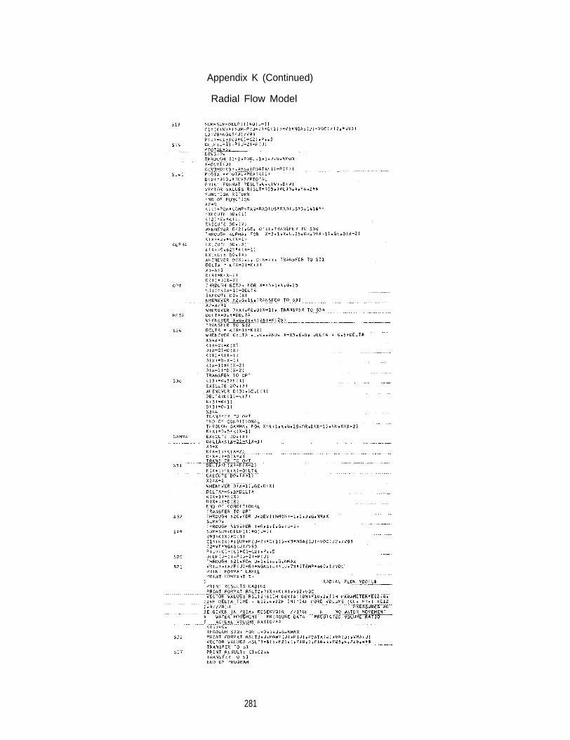
Appendix K (Continued)
Radial Flow Model
281
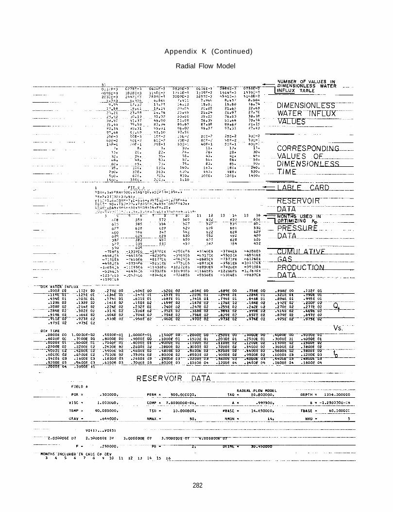
Appendix K (Continued)
Radial Flow Model
282
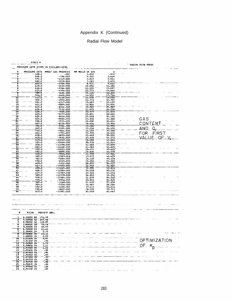
Appendix K (Continued)
Radial Flow Model
283
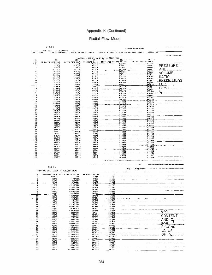
Appendix K (Continued)
Radial Flow Model
284

Appendix K (Continued)
Radial Flow Model
285

Appendix K (Continued)
Radial Flow Model
286

Appendix K [Continued)
Radial Flow Model
287

Appendix K (Continued)
Radial Flow Model
288

This Page Intentionally Left Blank
Except for the deletion of the dimensionless water influx and dimensionless time values
and the addition of the aquifer width, the input information required by the linear flow model is
the same as the radial flow model. The required information is listed below:
1. Reservoir and fluid characteristics: aquifer width, porosity, permeability, aquifer
thickness, reservoir depth (if well head pressures are given), water viscosity, effective
rock and water compressibility, constants a and b in gas compressibility factor correla-
tion, reservoir temperature, gas sand thickness, pressure base for gas measurement,
temperature base for gas measurement, gas gravity, number of time intervals, number
of months used in optimizing Kp’, number of initial pore volume values to be evaluated,
the values of the initial pore volumes to be investigated, designation if pressure is
given as well head or well bottom and as psig or psia, number of days in each time step.
The time increments to be used in optimizing the coefficient Kp‘.
The reservoir pressure data.
The cumulative gas production schedule.
2.
3.
4.
APPENDIX L
Computer Program for Linear Flow Model
The MAD program, input format and a list of the required information for the linear
model is given in this appendix. The reader should refer to Appendix K for a description of the
nomenclature. The data for Field A is processed and the results presented at the end of the
appendix as the example problem.
The following information, the same as for the radial model, is calculated from the
above data:
1. Reservoir bottom hole pressures, psia, from well head pressures.
2. Pound moles of gas in place for each time interval.
3. Reservoir pressures for no water movement.
4. Optimum value of Kp' for a given Vo, initial pore volume.
5. Reservoir pressure, psia, resulting from gas injection-production schedule and water
movement.
6. Current to initial pore volume ratios for the measured reservoir pressures for each
time step.
7. Current to initial pore volume ratios for the observed reservoir pressure data for each
time step.
Deck Assembly
1.
2.
3.
IBM center control cards
Linear Flow Model Program (MAD or Binary Deck)
Data289
The data is assembled as follows:
See Appendix K for description of format field specifications.
290
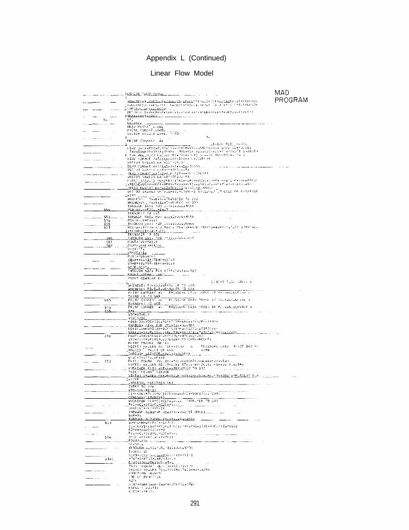
Appendix L (Continued)
Linear Flow Model
291

Appendix L (Continued)
Linear Flow Model
292
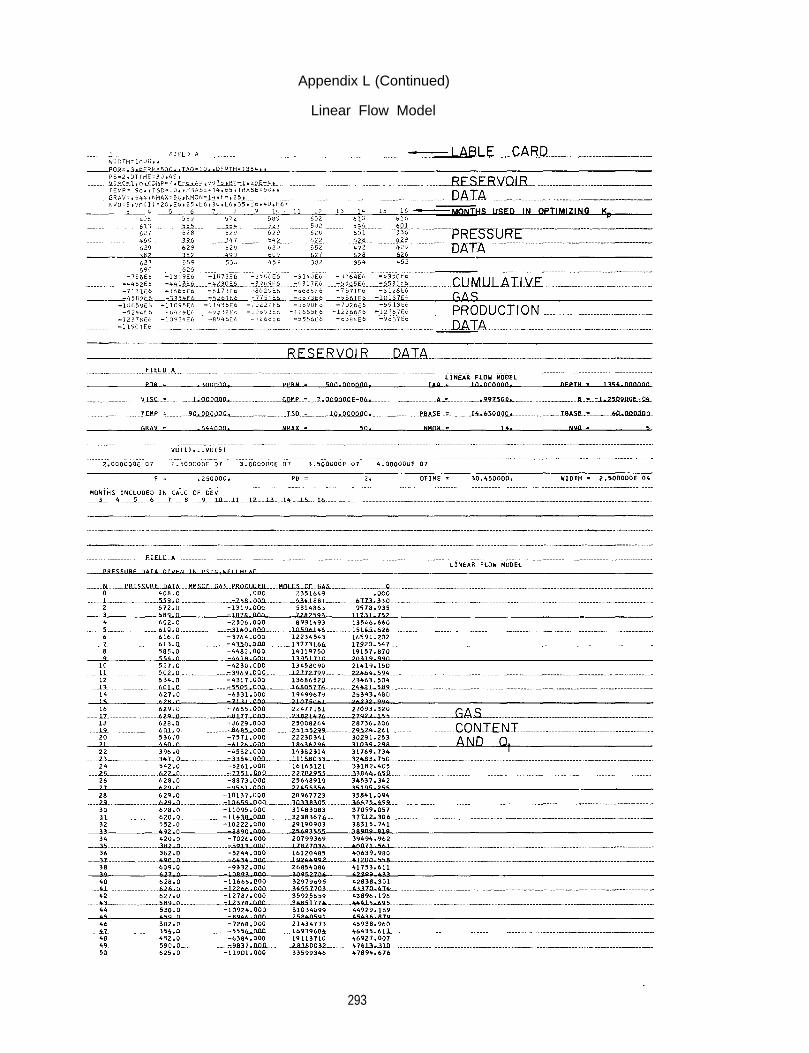
Appendix L (Continued)
Linear Flow Model
293
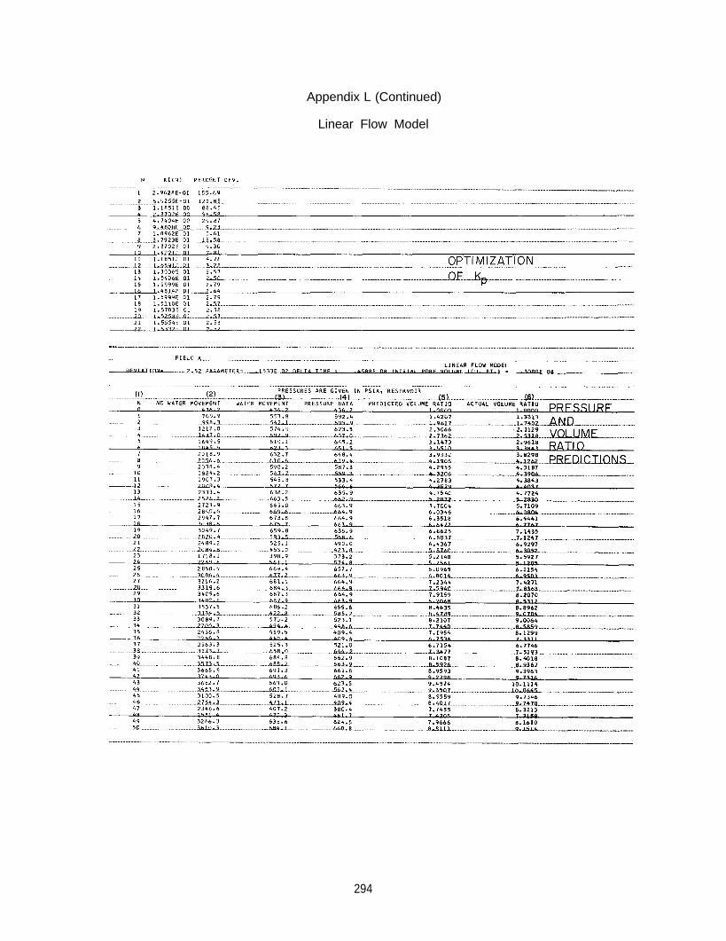
Appendix L (Continued)
Linear Flow Model
294

APPENDIX M
Computer Program for Resistance Function MethodIncluding Moving Boundary Modification
The MAD (Michigan Algorithmic Decoder) program as used for processing data by the
resistance function method for both the fixed and moving boundary cases is listed below, along
with the data input and printout for Field A. However, a list of symbols used in the program and
their meanings will be presented first, followed by a summary of the data input deck, and a more
detailed discussion of the use of the input.
Nomenclature of Symbols used in Resistance Function Method Program
A
AREA
B
COMPRS
DEL TIM
DEPTH
DE
DEV
DIM
DPD
D
DZ
ECORR
EP
E
ETEMP
EXPT
FRACTN
F
G
HEIGHT
HGAS
factor for gas compressibility: Z = A + B* P
area normal to the water flow in linear model
gas compressibility factor in Z = A + B *P, ps i - 1
combined water and formation compressibility, vol/(vol-psi)
number of days per time increment, ( = At)
depth of well, feet
water influx rate, ew ft3/day (In output printed by the program, ew is given
as thousands of cubic feet/day. )
sum of the absolute deviations between observed and calculated pressures, psi
dimension vector for dimensionless pressure array
dimensionless pressure difference, ∆ P t
percentage deviation between observed and calculated pressures
AZ in resistance function
water influx rate modification factor for moving boundary case (= β in Chapter
8). ECORR = 1.0 for fixed boundary
factor for relaxation of restriction on resistance curve, ( = in Chapter 6)
cumulative water influx, W e’ cubic feet (In the program printout E is given as
thousands of cubic feet. )
temporary value of E in iterative process in moving boundary case
exponent a for volume-radius relationship in moving boundary case
fraction of largest gas bubble volume encountered to be used as reference gas bub-
ble volume in moving boundary case
fraction of a complete circle open to flow
gas gravity (air = 1.0)
thickness of aquifer sand, feet
thickness of gas sand, feet
295

I
K
L
MODEL
MONTH
M
N
PARAM
PBASE
PCALC
PDATA
PDIM
PD
PERM
POROSY
PRCASE
P
PSTAR
Q
RADIUS radius of gas bubble
TBASE temperature base for gas, OR
TDIM dimensionless time
TD dimensionless time
index
group to be optimized (=Kr in Chapter 6)
total number of data points read in
= 1, for radial model fit
2, for thick sand model fit
3, for linear model fit
4, for variable radius case
101, for finite aquifer prediction (2nd pass)
102, for infinite aquifer prediction (2nd pass)
103, for linear aquifer prediction (2nd pass)
104, for finite variable radius case
105, for infinite variable radius case
number of time interval used in comparison of calculated and observed pressures
for optimization of Kr
number of the last time increment used for one of the geometric models
(= MONTH(NMONTH))
index
ratio of h/rb for thick sand model
pressure base for gas
calculated reservoir pressure, psia
pressure data, psig or psia, well head or well bottom
dimensionless pressure in table
dimensionless pressure, Pt, found by linear interpolation from table values: PDIM
aquifer permeability, md.
aquifer porosity, fraction void space
= 1, for well head, psig PDATA
2, for well head, psia PDATA
3, for well bottom, psig PDATA
4, for well bottom, psia PDATA
“observed” reservoir pressure, psia
“reference” dimensionless pressure for variable radius case
cumulative gas production, GP,
Q = MMSCF)
SCF at PBASE and TBASE. (In program output
296

TEMP reservoir temperature
TSTAR dimensionless time corresponding to “reference” gas bubble in variable radius case
VISCOSITY water viscosity, cp.
VLARGE largest gas bubble volume encountered in variable radius case
VMAX maximum number of Vo trials to be made
VRCALC calculated volume ratio (V/Vo)
VROBS observed volume ratio
VSTAR volume of “reference” gas bubble in variable radius case, cubic feet
WIDTH width of linear aquifer, feet
Z resistance function, psi/( cubic feet/ day)
Deck Assembly
1.
2.
3.
IBM center control cards
Resistance function program (MAD or binary deck)
Data
The data is assembled as follows:
PRCASE = 1, for WH, psig data2, for WH, psia data3, for WB, psig data4, for WB, psia data
MODEL = 1, for radial model fit2, for thick sand model fit3, for linear model fit4, for variable radius case fit (radial model)101, for finite aquifer prediction102, for infinite aquifer prediction103, for linear aquifer prediction104, for finite aquifer variable radius case
* See Appendix K for a description of the format.
297
MODEL = 105, for infinite aquifer, variable radius case
Unless otherwise specified by “Read Data” card, the following values are preset by the program:
EP = 0.02HGAS = HEIGHTMODEL = 1EXPT = 1.0FRACTN = 0.5K is optimized for best fit of pressuresVSTAR not specified, for use with models 104 and 105 onlyWIDTH is not specified; for use with linear model only
All the above values, except for K, are repeated for multiple VZERO values. Therefore desired
changes for multiple VZERO values must be specified.
Z(1). . . Z(M) values are to be read in only for “predictions”; i. e., for MODEL = 101,
102. . .105.
298
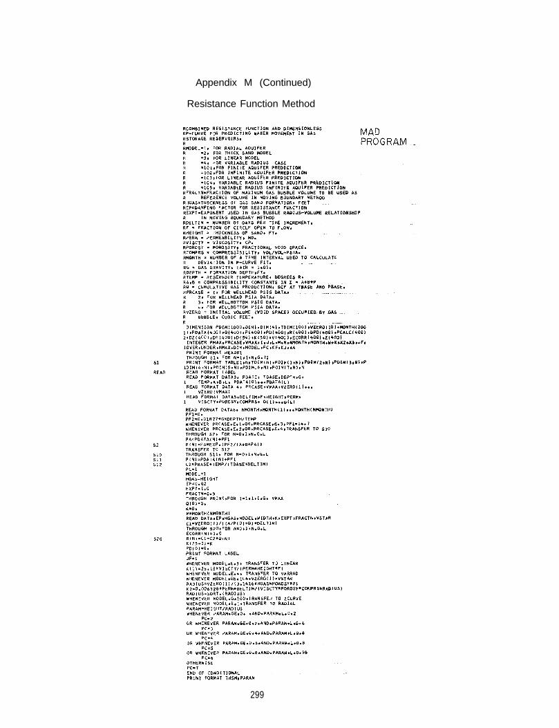
Appendix M (Continued)
Resistance Function Method
299

Appendix M (Continued)
Resistance Function Method
300

Appendix M ( Continued)
Resistance Function Method
301

Appendix M (Continued)
Resistance Function Method
302

Appendix M (Continued)
Resistance Function Method
303

Appendix M (Continued)
Resistance Function Method
304

Appendix M (Continued)
Resistance Function Method
305

Appendix M (Continued)
Resistance Function Method
306

Appendix M (Continued)
Resistance Function Method
307
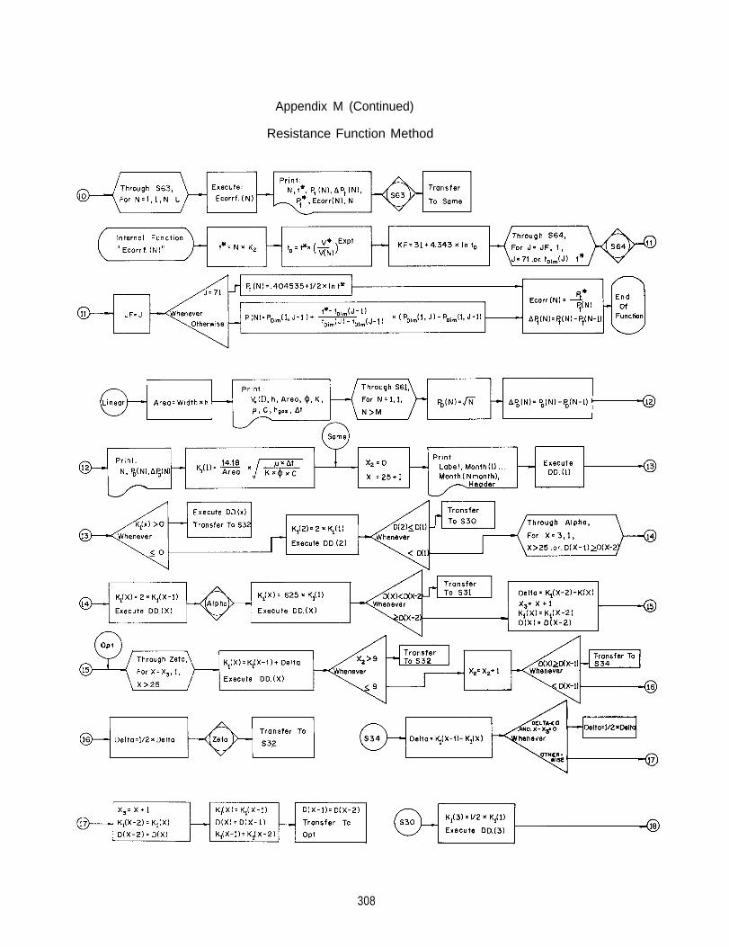
Appendix M (Continued)
Resistance Function Method
308

Appendix M (Continued)
Resistance Function Method
309
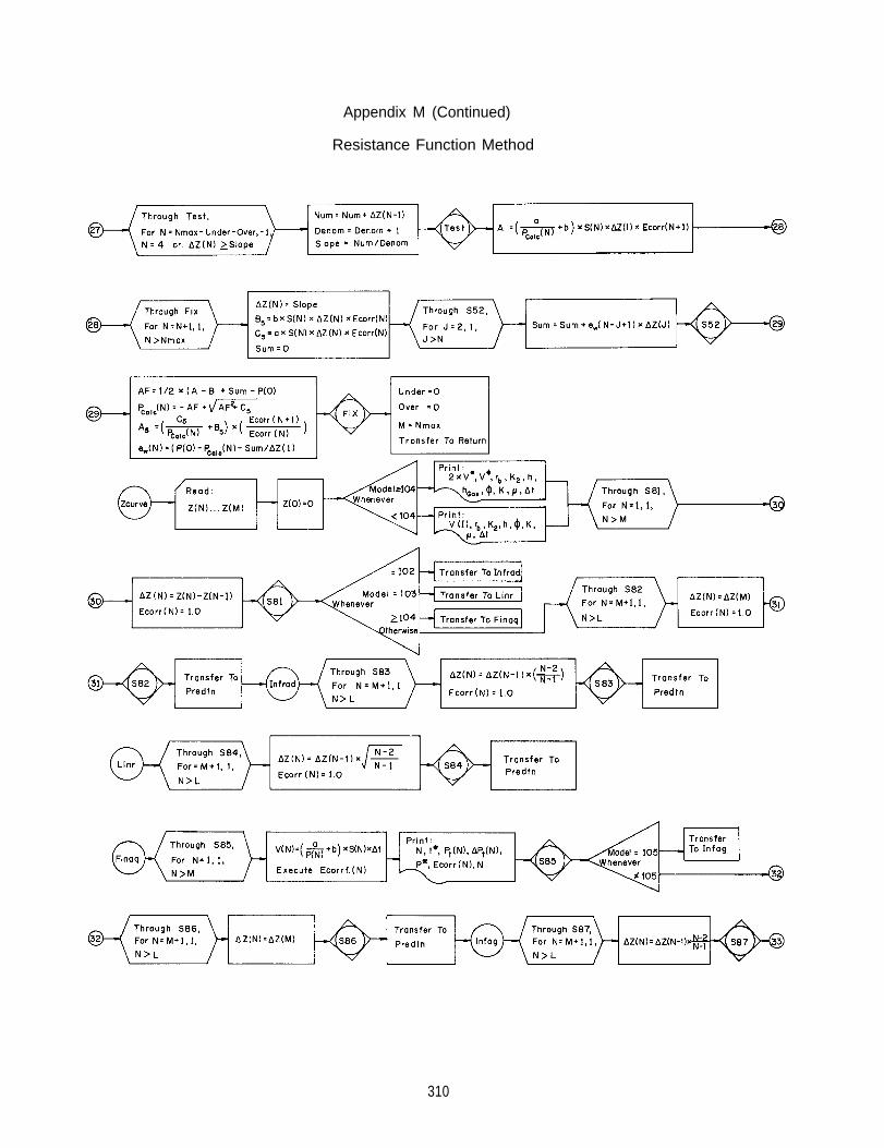
Appendix M (Continued)
Resistance Function Method
310
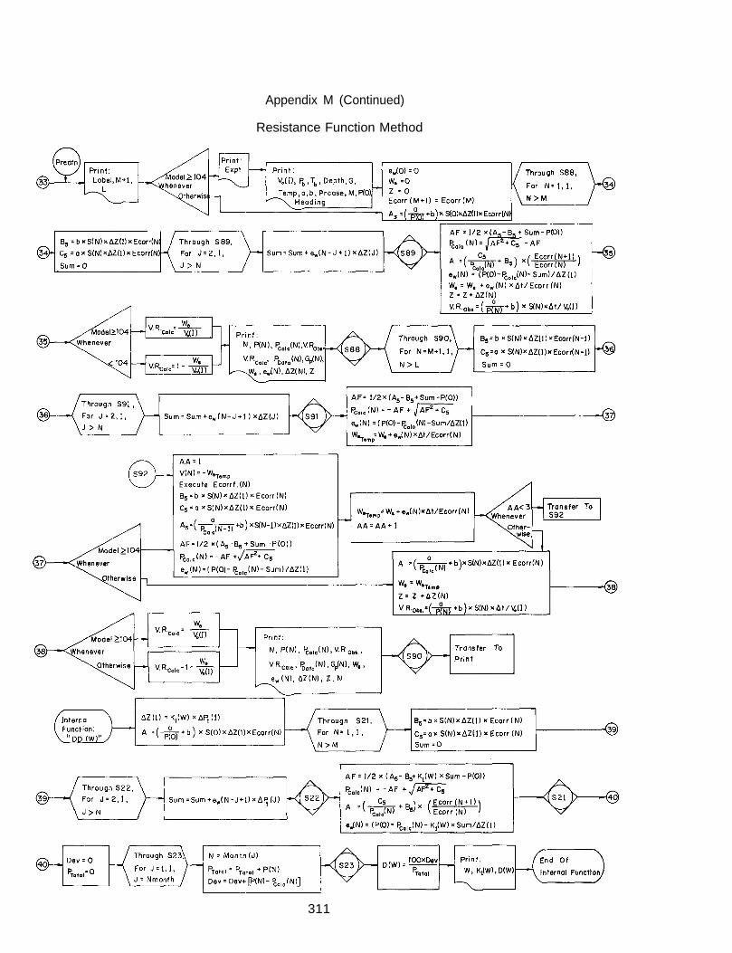
Appendix M (Continued)
Resistance Function Method
311

This Page Intentionally Left Blank
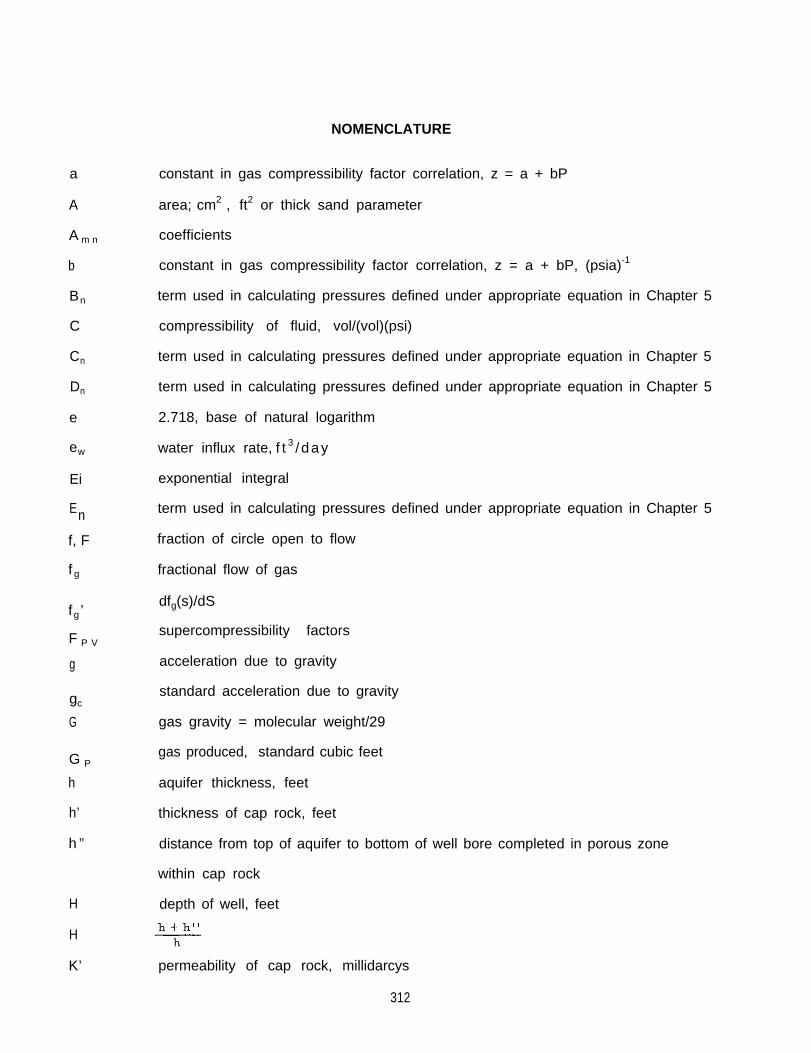
a
A
A m n
b
Bn
C
Cn
Dn
e
ew
Ei
En
f, F
f g
fg ’
F P V
g
gc
G
G P
h
h’
h ”
H
H
K’
NOMENCLATURE
constant in gas compressibility factor correlation, z = a + bP
area; cm2 , ft2 or thick sand parameter
coefficients
constant in gas compressibility factor correlation, z = a + bP, (psia)-1
term used in calculating pressures defined under appropriate equation in Chapter 5
compressibility of fluid, vol/(vol)(psi)
term used in calculating pressures defined under appropriate equation in Chapter 5
term used in calculating pressures defined under appropriate equation in Chapter 5
2.718, base of natural logarithm
water influx rate, f t 3 / day
exponential integral
term used in calculating pressures defined under appropriate equation in Chapter 5
fraction of circle open to flow
fractional flow of gas
dfg(s)/dS
supercompressibility factors
acceleration due to gravity
standard acceleration due to gravity
gas gravity = molecular weight/29
gas produced, standard cubic feet
aquifer thickness, feet
thickness of cap rock, feet
distance from top of aquifer to bottom of well bore completed in porous zone
within cap rock
depth of well, feet
permeability of cap rock, millidarcys
312

K, k
K, k
KP
Kr
K r ’
K v
n
log
L
m
M
n
P
‘base
p D
Pm,Pn
P t
P w h
∆ P’
qT
Q
Qt
r
r b
permeability, darcys, millidarcys
permeability, darcys, millidarcys
coefficient used in water flow equation for constant terminal pressure case
coefficient used in water flow equation for constant terminal rate case
ratio of vertical to horizontal permeability
vertical permeability, millidarcys
distance, feet or focul length of ellipse
log base e
log base 10
length, centimeter
reciprocal slope of p/z versus Gp plot, standard cubic feet/psi (or mobility ratio,
Appendix J)
thick sand parameter, M = (or slope of cap rock)
pound moles of gas at pressure, P, and temperature, T, cubic feet
pressure, atm, psia
pressure base, atm, psia
dimensionless pressure - see Chapter 3 for specific definition for a given flow
model
Legendre Polynomials of degree 0-5.
dimensionless pressure drop
well head pressure, psig
relationship defined by Equation 5-28a
fluid flow rate, cc/sec, cubic feet per day
2 π hrv/fg (Appendix J)
gas flow rate measured at base pressures, cubic feet per day
dimensionless water influx
radius, feet
radius of gas bubble or inner radius of aquifer, feet
313

r b *
r D
r e
R
°R
S
S
t
t D
T
Tb
U,V
V
v T
V
V r
V S
∆ V’
W
We
x,y ,z
Y
Z
Z
α
Y
reference gas bubble radius used in moving boundary problem
dimensionless radius, rD = r/rb
radius of exterior boundary of aquifer, feet
ratio of the radius of the exterior boundary, r e’ of the aquifer to the inner radius
of the aquifer, rb (or gas constant =
degrees Rankine
Laplace transform of dimensionless time, tD
nRT (or gas saturation, Appendix J)
time, day
dimensionless time
temperature, degrees Rankine
temperature base, degrees Rankine
constant used in specifying ellipse
velocity of fluid, centimeter per second, feet per day
total fluid velocity
gas reservoir volume, cubic feet
volume corresponding to rb*
gas research volume, cubic feet
specific volume
relationship defined by Equation 5-24
width gas bubble, feet
cumulative water influx, cubic feet
space coordinates
distance between the apex of the cap rock and the gas-water interface
gas compressibility factor, dimensionless
resistance function
parameter used in moving boundary problem to define reservoir shape
specific weight, pound forcer per cubic feet, y =
314
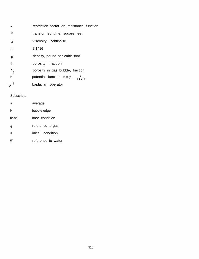
θ
µ
π
p
Subscripts
a
b
base
g
0
W
restriction factor on resistance function
transformed time, square feet
viscosity, centipoise
3.1416
density, pound per cubic foot
porosity, fraction
porosity in gas bubble, fraction
potential function,
Laplacian operator
average
bubble edge
base condition
reference to gas
initial condition
reference to water
315

REFERENCES
1. Bell, J. S. , and Shepherd, J. M., Pressure Behavior in the Woodbine Sand, Trans. AIME,192, 19 (1951).
2. Berry, V. J., Jr., and Pendergrass, J. D., Solution of Reservoir Transient Flow Problemson a Small Computer, Presented at Petroleum Production and Reservoir EngineeringSeminar, IBM Data Process Div., IBM Customer Executive Program (Feb 27. - Mar.1, 1962).
3. Bruce, W. A., An Electrical Device for Analyzing Oil-Reservoir Behavior, Trans. AIME,151, 73 (1943)
4. Calhoun, J. C., Jr., Fundamentals of Reservoir Engineering, Norman: University ofOklahoma Press, 1953.
5. Chatas, A. T. , A Practical Treatment of Nonsteady-State Flow Problems in Reservoir Sys-tems, Pet. Engr., 25 (5): B42; 25 (6): B38; 25 (9): B44 (1953).
6. Coats, K.H., Prediction of Gas Storage Reservoir Behavior, Ph. D. Thesis, University ofMichigan (1959).
7. Coats, K. H. , Tek, M. R. , and Katz, D. L. , Unsteady State Liquid Flow Through PorousMedia Having Elliptic Boundaries, Pet. Trans. AIME, 216, 460 (1959).
8. Coats, K. H., Tek, M. R., and Katz, D. L., Method for Predicting the Behavior of MutuallyInterfering Gas Reservoirs Adjacent to Common Aquifer, Pet. Trans. AIME, 216 , 247(1959).
9. Coats, K. H., A Mathematical Model for Water Movement about Bottom Water-Drive Reser-voirs, Soc Pet. Engr. Jour. 2 (NO. 1) p. 44 (1962).
10. Craft, B. C., and Hawkins, M. F., Jr., Applied Petroleum Reservoir Engineering, EnglewoodCliffs, N. J., Prentice-Hall, Inc. , 1959.
11. Darcy, Henry, Darcy’s Law, Les Fountaines Publiques de la Ville de Dijon, Victor Dalmont,Paris, 1856.
12. Dodson, C. R., and Standing, M. B., Pressure-Volume-Temperature and Solubility Relationsfor Natural Gas Water Mixtures, API Drill. Prod. Practice, 173 (1944).
13. Elkins, L. F. , Fosterton Field--An Unusual Problem of Bottom Water Coning and VolumetricWater Invasion Efficiency, Pet. Trans. AIME, 216, 130 (1959)..
14. Fatt, I., Pore Volume Compressibilities of Sandstone Reservoir Rocks, Trans. AIME, 213362 (1958).
15. Geertsma, J., The Effect of Fluid Pressure Decline on Volumetric Changes of Porous Rocks,Trans, AIME, 210, 331 (1957).
16. Glass, E. D., and Hessing, R. C., A Method of Computing Pressure Behavior and Volume ofGas Storage Reservoir, J. Pet. Tech., Vol. 14, No. 5, p. 554 (1962).
17. Hall, H. N. , Compressibility of Reservoir Rocks, Trans. AIME, 198, 309 (1953).
18. Hantush, M. S., and Jacob, C. E., Non-Steady Radial Flow in an Infinite Leaky Aquifer,Trans. AGU, 36, 95 (1955).
316
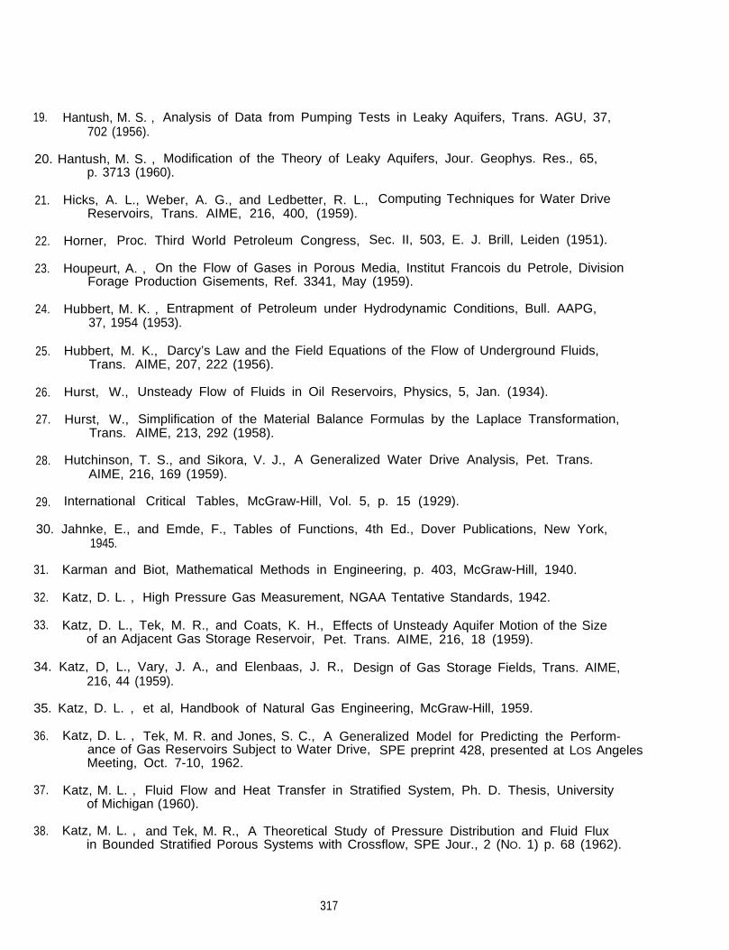
19. Hantush, M. S. , Analysis of Data from Pumping Tests in Leaky Aquifers, Trans. AGU, 37,702 (1956).
20. Hantush, M. S. , Modification of the Theory of Leaky Aquifers, Jour. Geophys. Res., 65,p. 3713 (1960).
21. Hicks, A. L., Weber, A. G., and Ledbetter, R. L., Computing Techniques for Water DriveReservoirs, Trans. AIME, 216, 400, (1959).
22. Horner, Proc. Third World Petroleum Congress, Sec. II, 503, E. J. Brill, Leiden (1951).
23. Houpeurt, A. , On the Flow of Gases in Porous Media, Institut Francois du Petrole, DivisionForage Production Gisements, Ref. 3341, May (1959).
24. Hubbert, M. K. , Entrapment of Petroleum under Hydrodynamic Conditions, Bull. AAPG,37, 1954 (1953).
25. Hubbert, M. K., Darcy’s Law and the Field Equations of the Flow of Underground Fluids,Trans. AIME, 207, 222 (1956).
26. Hurst, W., Unsteady Flow of Fluids in Oil Reservoirs, Physics, 5, Jan. (1934).
27. Hurst, W., Simplification of the Material Balance Formulas by the Laplace Transformation,Trans. AIME, 213, 292 (1958).
28. Hutchinson, T. S., and Sikora, V. J., A Generalized Water Drive Analysis, Pet. Trans.AIME, 216, 169 (1959).
29. International Critical Tables, McGraw-Hill, Vol. 5, p. 15 (1929).
30. Jahnke, E., and Emde, F., Tables of Functions, 4th Ed., Dover Publications, New York,1945.
31. Karman and Biot, Mathematical Methods in Engineering, p. 403, McGraw-Hill, 1940.
32. Katz, D. L. , High Pressure Gas Measurement, NGAA Tentative Standards, 1942.
33. Katz, D. L., Tek, M. R., and Coats, K. H., Effects of Unsteady Aquifer Motion of the Sizeof an Adjacent Gas Storage Reservoir, Pet. Trans. AIME, 216, 18 (1959).
34. Katz, D, L., Vary, J. A., and Elenbaas, J. R., Design of Gas Storage Fields, Trans. AIME,216, 44 (1959).
35. Katz, D. L. , et al, Handbook of Natural Gas Engineering, McGraw-Hill, 1959.
36. Katz, D. L. , Tek, M. R. and Jones, S. C., A Generalized Model for Predicting the Perform-ance of Gas Reservoirs Subject to Water Drive, SPE preprint 428, presented at LOS AngelesMeeting, Oct. 7-10, 1962.
37. Katz, M. L. , Fluid Flow and Heat Transfer in Stratified System, Ph. D. Thesis, Universityof Michigan (1960).
38. Katz, M. L. , and Tek, M. R., A Theoretical Study of Pressure Distribution and Fluid Fluxin Bounded Stratified Porous Systems with Crossflow, SPE Jour., 2 (NO. 1) p. 68 (1962).
317

39. Lefkovits, H. C. , Hazebroek, P., Allen, E. E., and Mathews, C. S., A Study of the Behaviorof Bounded Reservoirs Composed of Stratified Layers, Trans. AIME, 222, II-43 (1961).
40. Klinkenberg, L. S., The Permeability of Porous Media to Liquids and Gases, API Drill.Prod. Practice, 200 (1941).
41. McCarty, D. G. , and Barfield, E. C. , The Use of High Speed Computers for PredictingFlood Out Patterns, Trans. AIME, 213, 139 (1958).
42. McEven, C. R., Jr., Material Balance Computations with Water Influx in the Presence ofUncertainty in Pressure, Society of Petroleum Engineers Jour. , Vol. 2, No. 2, p. 120,June (1962).
43. Mortada, M. , A Practical Method for Treating Oilfield Interference in Water-Drive Reser-voirs, Trans. AIME 204, 217 (1955).
43a. Mueller, T. D., Transient Response of Nonhomogeneous Aquifers, Soc. Pet. Engr. Jour.,2, No. 1, p. 33 (1962).
44. Muskat, M., The Flow of Homogeneous Fluids Through Porous Media, Ann Arbor, J. W.Edwards, Inc., 1946.
45. Muskat, M., Physical Principles of Oil Production, New York, McGraw-Hill, 1949.
46. Nisle, R. G. , How to Use the Exponential Integral, The Petroleum Engineer, p. B- 171,August (1956).
47. Nisle, R. G. , The Effect of Partial Penetration in Pressure Build Up in Oil Wells, Trans.AIME, 213, 85 (1958).
48. Orifice Metering of Natural Gas, PRCI Gas Measurement Committee, Report 3, (1955).
49. Pendergrass, J. D., and Berry, V. J., Pressure Transient Performances of a MultilayeredReservoir with Crossflow, SPE Jr. , 2, No. 4, p. 347 (1962).
50. Pirson, S. J., Elements of Oil Reservoir Engineering, 2nd Ed., New York, McGraw-Hill,1958.
51. Rachford, H. H., Jr., Taylor, R. D., Douglas, J., Jr., and Dyke, P.M., Application ofNumerical Methods to Predict Recovery from Thin Oil Columns, Trans. AIME, 213193 (1958).
52. Robinson, M. P., Pressure Interference Correction to the Material Balance Equation forWater Drive Reservoirs Using a Digital Computer, Trans. AIME, 213, 418 (1958).
53. Russell, D. G., and Prats, M., Performance of Layered Reservoirs with Crossflow--Single-Compressible Fluid Case, SPE Jour., 2, No. 1, p. 53 (1962).
54. Russell, D. G., and Prats, M., The Practical Aspects of Interlayer Crossflow, J. Pet.Tech., 14, No. 6, p. 589 (1962).
55. Rzepczynski, W., Katz, D. L., Tek, M, R. and Coats, K. H., The Mt. Simon Storage Reser-voir in the Herscher Field, Presented at Research Conference on Underground Storageof Natural Gas, University of Michigan, Ann Arbor, Michigan, July 16-17, 1959.Oil and Gas Jr. , 59, No. 25, 86 (1961).
56. Sarem, A.M., Z-Factor Equation Developed for use in Digital Computers, The Oil andGas Jour. , Vol. 59, No. 38, p. 118, Sept. (1961).
318

57. Schilthuis, R. G., and Hurst, W. , Variations in Reservoir Pressure in the East TexasField, Pet. Trans. AIME, 114, 164 (1935).
58. Schneebeli, G., Sur la Theorie des Ecoulements de Filtration, La Honille Blanche NOSpecial A, 186 (1953).
59. Sneddon, I. N., Fourier Transforms, McGraw-Hill, 1951,
60. Tek, M. R., Grove, M. L., and Poettmann, F. H., Method for Determining the Back-PressureBehavior of Low Permeability Natural Gas Wells, AIME Trans., 207 (1956).
61. Tek, M. R., Development of a Generalized Darcy Equation, Trans. AIME, 210, 376 (1957).
62. Tek, M. R., Coats, K. H., and Katz, D. L., The Effect of Turbulence on Flow of NaturalGas Through Porous Reservoirs, J. Pet, Tech., 14 (No. 7) p. 799 (1962).
63. Theis, C. V. , The Relation Between the Lowering of the Piezometric Surface and the Rateand Duration of Discharge of a Well using Ground-Water Storage, Trans. AmericanGeophys. Union, 16, 519 (1935).
64. Van Everdingen, A. F. , and Hurst, W. , The Application of the Laplace Transformation toFlow Problems in Reservoirs, Trans. AIME, 186, 305 (1949).
65. Van Meurs, P., The Use of Transparent Three-dimensional Models for Studying the Mechanismof Flow Processes in Oil Reservoirs, Trans. AIME, 210, 295 (1957).
66. Walton, W. C., Leaky Artesian Aquifer Conditions in Illinois, RI 39, State Water Soc. (1960).
67. Warren, J. E., The Unsteady State Behavior of Linear Gas Storage Reservoirs, Pet, Engr.,38, No. 12, 60 (1956).
67a. Welge, H. J. , A Simplified Method for Computing Oil Recoveries by Gas or Water Drive,Trans. AIME, 195, 91 (1952).
68. Witherspoon, P. A., and Mueller, T. D., Evaluation of Underground Gas-Storage Conditionsin Aquifers through Investigations of Ground Water Hydrology, J. Pet. Tech., Vol. 14,No. 5, p. 555 (1962).
69. Witherspoon, P. A., and Nelson, C. G., Caprock Evaluation for Aquifer Storage, Presentedbefore American Gas Association (1962).
70. Woods, E.G. and Comer, A. G., Saturation Distribution and Injection Pressure for a RadialGas Storage Reservoir* J, Pet. Tech., Vol. 14, No. 12, p, 1389, 1962.
71. Woody, L. D., Jr., and Moore, W. D., Performance Calculations for Reservoirs withNatural or Artificial Water Drives, Trans. AIME, 210, 245 (1957).
72. Yoo, H. D., Katz, D. L., and Tek, M. R., Study of Gas Reservoirs Subject to Water Driveon Electronic Differential Analyzer, Jour. SPE, 1, No. 4, p. 287, Dec. (1961).
319

The following progress reports have been written during the course of the project, with
copies distributed to the Pipeline Research Council International, Inc. Committees:
1. Engineering Studies on Movement of Water in Contact with Natural Gas -- FirstProgress Report, Katz, D. L., Tek, M. R., Coats, K. H., and Katz, M. L.,Sept. 14, 1959.
2. Engineering Studies on Movement of Water in Contact with Natural Gas -- SecondProgress Report, Katz, M. L., Coats, K. H., Tek, M. R., and Katz, D. L., June18, 1960.
3. Engineering Studies on Movement of Water in Contact with Natural Gas -- FirstAnnual Report, Katz, D. L., Tek, M. R., Coats, K. H., and Katz, M. L., Sept.1960.
4. Engineering Studies on Movement of Water in Contact with Natural Gas -- SecondAnnual Report, Katz, D. L. , Tek, M. R. , Miller, M. C. , and Jones, S. C. , Oct. 1961.
Since copies of these reports are no longer available, they are not listed as references.
320

This Page Intentionally Left Blank
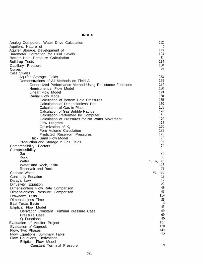
INDEX
Analog Computers, Water Drive CalculationAquifers, Nature ofAquifer Storage, Development ofBarometer Correction for Fluid LevelsBottom-Hole Pressure CalculationBuild-up TestsCapillary PressureCurvesCase Studies
Aquifer Storage FieldsDemonstrations of All Methods on Field A
Generalized Performance Method Using Resistance FunctionsHemispherical Flow ModelLinear Flow ModelRadial Flow Model
Calculation of Bottom Hole PressuresCalculation of Dimensionless TimeCalculation of Gas in PlaceCalculation of Gas Bubble RadiusCalculation Performed by ComputerCalculation of Pressures for No Water MovementFlow DiagramOptimization of KpPore Volume CalculationPredicted Reservoir Pressures
Thick Sand Flow ModelProduction and Storage in Gas Fields
Compressibility FactorsCompressibility
GasRockWaterWater and Rock, InsituReservoir and Rock
Connate WaterContinuity EquationDarcy’s LawDiffusivity EquationDimensionless Flow Rate ComparisonDimensionless Pressure ComparisonDrawdown TestsDimensionless TimeEast Texas BasinElliptical Flow Model
Derivation Constant Terminal Pressure CasePressure CaseQ Functions
Evaluation of Aquifer ProjectEvaluation of CaprockFlow, TWO PhasesFlow Equations, Summary TableFlow Equations, Derivations
Elliptical Flow ModelConstant Terminal Pressure
1522
113124
81114150
79
23315518418017315816517016517016117017316017217117319974
7380
5, 6, 75113
7878, 80
1917224545
11425
443696945
127120149
92
69
321

Hemispherical Flow ModelConstant Terminal Pressure
Linear Flow ModelConstant Terminal PressureConstant Terminal Rate
Radial Flow ModelConstant Terminal Pressure
Finite AquiferInfinite Aquifer
Constant Terminal RateFinite AquiferInfinite Aquifer
Fluid PropertiesGas- Water Contact, Location ofHemispherical Flow Model
Case StudyDiffusivity EquationPressure Case
Example ProblemRate Case
Example ProblemInitial Gas InjectionInitial Gas Pore VolumeInsitu Compressibility and Permeability Pump Tests
Example ProblemInterference Between Gas FieldsLinear Flow Model
Case StudyComputer ProgramConstant Terminal Rate Case
Example ProblemLimited Reservoir
Constant Terminal Pressure CaseExample ProblemLimited Reservoir
Diffusivity EquationSteady State
Location of Gas- Water Contact (Bubble Edge)Example Problem
Low Permeability or Non-Uniform SandMichigan Stray SandMoving Boundary Approximation Based on Hemispherical Model
Calculation ProceduresMoving Boundary Problem in Aquifer StorageNomenclatureOptimization, Effective Values of Kr and KpOptimization, Initial Gas Pore VolumePermeability MeasurementPermeability, Determination of InsituPound Day ConceptPrediction of Gas Reservoir Performance
Variable Rate CaseVariable Pressure Case
Pressure Distribution, Variation with Time for AquifersPressure Gradients in Aquifer
Example Problem
65
5957
5652
544973
133
1804043434142
12983
113117145
173289
2931323434342935
13313782
5142144139312
979918
114139
959597
7132132
322

PressuresObservation Wells
Radial Flow ModelCase StudyComputer ProgramConstant Terminal Pressure Case
Example ProblemConstant Terminal Rate Case
Example ProblemDerivations of EquationsDiffusivity EquationSteady State
ReferencesReservoir Pressure, Calculation from Well Head PressureResistance Function
Calculation from Field DataCase StudyComputer ProgramConceptExtrapolation of the Resistance Function CurveLogicSelf Correcting Features of the Computational ProcedureSteps for Calculating Field Performance
Rock CompressibilitySteady State
Radial Flow ModelLinear Flow Model
Stratified FlowSuperposition Principle
Application to Flow EquationExample Problem
System CalculationTemperature-ReservoirThick Sand Model
Case StudyDerivation of EquationDiffusivity EquationExample Problem
Threshold PressureTwo Phase FlowViscosity
BrineWater
WaterCompressibilityMovement CalculationViscosity
82
158276
27282526492328
31681
101103184295102110101109105
80
2835
1478891931581
176603538
11, 150149, 272
7775
7513075
323

This Page Intentionally Left Blank

This Page Intentionally Left Blank

Copyright, 2003 All Rights Reserved by Pipeline Research Council International, Inc.
PRCI Reports are Published by Technical Toolboxes, Inc.
3801 Kirby Drive, Suite 340 Houston, Texas 77098 Tel: 713-630-0505 Fax: 713-630-0560 Email: [email protected]


