
Multidecadal Evaluation of WRF Downscaling Capabilities over WesternAustralia in Simulating Rainfall and Temperature Extremes
JULIA ANDRYS AND THOMAS J. LYONS
State Centre of Excellence for Climate Change, Woodland and Forest Health,
Murdoch University, Perth, Western Australia, Australia
JATIN KALA
The Australian Research Council Centre of Excellence for Climate System Science, and Climate Change
Research Centre, University of New South Wales, Sydney, New South Wales, Australia
(Manuscript received 15 August 2014, in final form 31 October 2014)
ABSTRACT
The authors evaluate a 30-yr (1981–2010) Weather Research and Forecast (WRF) Model regional climate
simulation over the southwest of Western Australia (SWWA), a region with a Mediterranean climate, using
ERA-Interim boundary conditions. The analysis assesses the spatial and temporal characteristics of climate
extremes, using a selection of climate indices, with an emphasis on metrics that are relevant for forestry and
agricultural applications. Two nested domains at 10- and 5-km resolution are examined, with the higher-
resolution simulation resolving convection explicitly. Simulation results are compared with a high-resolution,
gridded observational dataset that provides daily rainfall, minimum temperatures, and maximum tempera-
tures. Results show that, at both resolutions, the model is able to simulate the daily, seasonal, and annual
variation of temperature and precipitation well, including extreme events. The higher-resolution domain
displayed significant performance gains in simulating dry-season convective precipitation, rainfall around
complex terrain, and the spatial distribution of frost conditions. The high-resolution domain was, however,
influenced by grid-edge effects in the southwestern margin, which reduced the ability of the domain to rep-
resent frontal rainfall along the coastal region. On the basis of these results, the authors feel confident in using
the WRF Model for regional climate simulations for the SWWA, including studies that focus on the spatial
and temporal representation of climate extremes. This study provides a baseline climatological description at
a high resolution that can be used for impact studies and will also provide a benchmark for climate simulations
driven by general circulation models.
1. Introduction
Changes in climate extremes are of particular interest
because of their disproportionately large influence on
ecosystems, agriculture, and human health (Patz et al.
2005; Easterling et al. 2000). The southwest of Western
Australia (SWWA) has been identified as a region that
is acutely at risk of climatic change (Hughes 2003;
Malcolm et al. 2006); there is limited knowledge on how
these changes are likely to manifest at the regional scale,
however, in particular with respect to extremes. Forestry
and agriculture encapsulate the majority of the land use
in the SWWA and contribute significantly to regional
prosperity. For example, cereal crops, the largest agri-
cultural sector in the state, contribute AUD 4.5 billion
annually to the Western Australian economy (Varnas
2014). Understanding how these industries may be im-
pacted by changes in climate extremes is critical for
developing management strategies that will enable ad-
aptation and preserve this prosperity.
Niu et al. (2014) reviewed the current understanding
of plant responses to climate extremes, including heat
waves, frost, drought, and flooding, and found that,
while the response was not uniform between ecosys-
tems, extreme events generally have a deleterious effect
on plant productivity and survivability. The negative
response to drought and heat stress for forests globally
is supported by Allen et al. (2010) and Clifford et al.
(2013). When examining forest mortality events in the
SWWA, Evans and Lyons (2013) found that sudden
Corresponding author address: Julia Andrys, Murdoch Univer-
sity, 90 South St., Murdoch WA 6150, Australia.
E-mail: [email protected]
370 JOURNAL OF APPL IED METEOROLOGY AND CL IMATOLOGY VOLUME 54
DOI: 10.1175/JAMC-D-14-0212.1
� 2015 American Meteorological Society

increases in the diurnal temperature range were
a significant factor in forest-mortality events, whereas
Brouwers et al. (2012) established that the combination
of drier-than-average conditions followed by heat-wave
events also led to an episode of widespread decline
within the native forest. Because forest ecosystems have
acclimated to the prevailing conditions, extreme events
tend to cause damage to the biota by increasing stress on
the vegetation, making it less able to withstand other
stresses such as, for example, attacks by bark beetles
(Williams et al. 2012).
The response of agricultural production, particularly
cereal crops, to extreme conditions is more temporally
dependent and is linked with the growing cycle. Frost or
high temperatures that occur in the grain-filling period
of the crop-growth cycle, for example, will result in the
most significant reduction in agricultural yield (Asseng
et al. 2012; Ludwig and Asseng 2006; Zheng et al. 2012).
It is therefore clear that assessments of future changes in
climate on agriculture and forestry need to focus on
climate extremes, with a particular focus on the magni-
tude and timing of these events.
Investigating changes in extremes of both temperature
and precipitation is difficult within the constructs of
general circulation models (GCMs) because their reso-
lution does not allow for the adequate representation of
finer-scale features, including topography and land
cover, and mesoscale weather systems, which play a sig-
nificant role in the development of extreme conditions
(Ekström et al. 2005; Fowler et al. 2005; Donat et al.
2010; Mishra et al. 2012). As such, downscaling tech-
niques, including dynamical downscaling, are frequently
applied to GCM output. The Weather Research and
Forecasting (WRF) Model (Skamarock et al. 2008) em-
ployed as a regional climate model (RCM) is one such
tool for this purpose. The ability of WRF to downscale
GCMs and to better account for regional climate has
been well established in simulations conducted over cli-
matological regions in Europe (Christensen et al. 2007;
Chu et al. 2010), North America (Mearns et al. 2009;
Patricola and Cook 2013), and Asia (Chotamonsak et al.
2011). A number of these studies have also included an
assessment of climate extremes (Argüeso et al. 2011;Gao et al. 2012; Salathé et al. 2010). To promote a con-
sistentmethod for regional downscaling experiments and
hence to improve the quality of experiment outcomes,
the Coordinated Regional Downscaling Experiment
(CORDEX; Giorgi et al. 2009) was established. The
CORDEX framework highlights the importance of first
validating the RCM configuration through the evalua-
tion of simulations with boundary conditions derived
from reanalysis data before simulations downscaling
GCM data are run.
Kala et al. (2015) examined a number of physics op-
tions for WRF in the SWWA for a 12-month period and
found that the model was sensitive to parameterization
options, in particular the choice of longwave and short-
wave radiation schemes, land surface model, and plane-
tary boundary layer scheme. Kala et al. (2015) also found
that at a 10-km resolutionWRFwas not able to represent
the magnitude of dry-season rainfall, and a systematic
underestimation of coastal precipitation was linked to
unresolved topography in the region. The influence of
unresolved topography on simulated precipitation is
supported by regional climate studies in other regions,
which have found that higher-resolution simulations
represent precipitation with greater skill (Cardoso et al.
2013; Warrach-Sagi et al. 2013).
In this study we aim to validate WRF as an RCM in
the SWWA that is forced by reanalysis data over a 30-yr
period between 1981 and 2010. We evaluate the ability
of WRF to simulate extremes of temperature and pre-
cipitation in the SWWA as the basis for ongoing re-
search to downscale an ensemble of GCMs to examine
the impact of future climate changes. To achieve this
aim, we consider the extent to which increasing the
resolution of the WRF simulation will improve simula-
tion of extremes. The ability of the simulation to detect
the daily, seasonal, and annual variability of the
SWWA is evaluated to ensure thatWRF can adequately
represent the climatological characteristics of the re-
gion. The spatial and temporal distribution of some ex-
treme precipitation and temperature indices are also
assessed.
2. Methods
a. Southwest Western Australia
SWWA is a region of high biological diversity
(Fitzpatrick et al. 2008), which also supports an urban
population in the coastal city of Perth and extensive rain-
fed cereal crops toward the interior. The growing season
for these crops is in the cooler months of May–October
(Ludwig andAsseng 2006). In the region, summer is from
December to February (DJF), autumn is from March to
May (MAM), winter is from July to August (JJA), and
spring is from September to November (SON). SWWA
experiences hot dry summers and cool wet winters, typ-
ical of its Mediterranean-type climate (Gentilli 1971,
108–114), but this type of climate in combinationwith low
soil fertility means that the biota and agricultural re-
sources of the region are highly susceptible to changes in
climate (Kingwell 2006).
The most influential large-scale driver of the SWWA
climate is the position of the subtropical high pressure
FEBRUARY 2015 ANDRYS ET AL . 371
belt (Gentilli 1971, 108–114). In the spring and summer,
the belt is positioned to the south of SWWA and advects
hot continental air to the coast while channeling the
passage of rain-bearing frontal systems to the south,
resulting in dry conditions. Summer rainfall is a result of
surface convection, cutoff lows (Pook et al. 2012), and
northwesterly cloud bands that bring rain to the interior
(Tapp and Barrell 1984). Infrequent, large-scale sum-
mer rain events in the SWWA, which occur only two or
three times in a decade, were described by Wright
(1974). Caused by meridional troughs passing over the
region, Wright (1974) found that these rain events often
took place when a former tropical cyclone was present
north of Western Australia. Previous studies assessing
WRF downscaling capabilities over the SWWA on
a seasonal time scale have found that the scarcity and
distribution of rain in the summer months is challenging
to represent accurately (Kala et al. 2015). In the winter
months the subtropical high pressure belt moves
northward, allowing for the passage of frontal systems
over the region that are the main source of annual
rainfall. Annual rainfall variability in the region is con-
siderable (Power et al. 1998) and has been found to be
influenced by large-scale teleconnections, such as the
Indian Ocean dipole (England et al. 2006).
SWWA is an area of low relief. The main topo-
graphical feature that influences the climate of the re-
gion is the Darling Scarp, which runs parallel to the
coast 25 km inland and results in a sudden change in
elevation of approximately 300m. This feature can be
seen in Fig. 1b. The meteorological influence of this
scarp has been shown to be difficult to represent in
mesoscalemodels with resolutions that aremore coarse
than 0.5 km (Pitts and Lyons 1990; Kala et al. 2011,
2015).
b. Model configuration
A 30-yr, three-domain regional climate simulation
from 1981 to 2010 was conducted using WRF, version
3.3, driven by ERA-Interim (Dee et al. 2011) boundary
conditions. A 3-month model spinup period was used.
The outer 50-km domain (Fig. 1a) was based on the
CORDEXAustralia domain. The two nested domains,
at 10- and 5-km resolution, were chosen to evaluate the
influence of spatial scale on model skill and also to
compare the performance of parameterized convec-
tion with convection that is explicitly resolved in the
model. We note that the downscaling ratio of 2 used
between our two nested domains is a lower ratio than is
usually employed by regional climate simulations.
Our choice of downscaling ratio between these do-
mains was based on the limits of the computational
resources available. This meant that the resolution of
the inner domain (5 km) matched the resolution of the
gridded observational dataset, which is discussed in
section 2c.
Parameterization options and model setup were based
on the findings of a prior sensitivity analysis of WRF to
different physics and input data over SWWA (Kala et al.
2015) and include the single-moment 5-classmicrophysics
scheme (Hong et al. 2004), RRTM for longwave radia-
tion (Mlawer et al. 1997), Dudhia shortwave radiation
(Dudhia 1989), Yonsei University planetary boundary
layer scheme (Hong and Lim 2006), convective parame-
terization on the first and second domains only from
Kain–Fritsch (Kain 2004), theMM5 surface-layer scheme
(Grell et al. 2000), and the Noah land surface model
(Chen and Dudhia 2001). (Acronym definitions can be
found at http://www.ametsoc.org/PubsAcronymList.)
The model employs 30 vertical levels, which are more
densely spaced near the surface, 150-day averaging for
deep soil temperatures, and spectral nudging for the
upper layers of the outer domain only. Carbon dioxide
concentrations were updated on amonthly frequency on
the basis of observations from Baring Head, New Zea-
land (Keeling et al. 2001), as being representative of the
Southern Hemisphere. A 10-gridpoint relaxation zone
was removed from the domain boundaries prior to
analysis of the results.
c. Observational data
Observational data used for evaluation come from
a daily gridded dataset of maximum and minimum tem-
peratures and rainfall provided by the Australian Bureau
of Meteorology (BoM) as a contribution to the Austra-
lian Soil Water Availability Project (AWAP; Raupach
et al. 2009). The AWAP temperature and precipitation
dataset, at a resolution of 5 km, is an interpolation from
a network of weather stations across Australia (Jones
et al. 2009) and has been used as a validation tool for
previous regional climate simulations inAustralia (Evans
andMcCabe 2010; Evans et al. 2012; Kala et al. 2015).We
note the uncertainties associated with the fitting of sur-
faces to the observations to yield the gridded dataset, but
the AWAP data have employed topography-resolving
analysis methods to minimize this uncertainty (Jones
et al. 2009). King et al. (2013) evaluated the merits
of the AWAP dataset to examine extreme-rainfall
characteristics and found that it demonstrated
good agreement with station data and was suitable
to examine extreme rainfall. King et al. (2013) did
suggest caution in using the AWAP data in areas of low
station density, but these regions are sufficiently re-
moved from the two innermost domains of this simu-
lation so as not to influence the quality of the
observational data for this study. The AWAP data are
372 JOURNAL OF APPL IED METEOROLOGY AND CL IMATOLOGY VOLUME 54

illustrated in Fig. 2, which shows the average seasonal
mean rainfall, maximum temperatures, and minimum
temperatures for 1981–2010. Precipitation (Fig. 2c)
is most heavily concentrated at the coast, and there
is a significant decline in rainfall as distance inland
increases.
d. Statistics and indices
The AWAP observations were interpolated using
simple inverse-distance weighting to the 5- (W5k) and
10-km (W10k) domains to enable intercomparison.
Daily variability was quantified using probability density
FIG. 1. RCM terrain for the (a) outer model domain, including the extent of the nested grids,
and (b) the higher-resolution terrain of domain 3.
FEBRUARY 2015 ANDRYS ET AL . 373

functions (PDFs). Because the observational data do
not include daily rainfall values of less than 0.2mm,
simulation values below this threshold have been re-
moved from the daily variability analysis. To establish
the spatial variability of the daily PDFs, the Perkins
skill score (PSS; Perkins et al. 2007) was employed,
which compares the observed and simulated probabil-
ity distributions:
FIG. 2. Climatological seasonal means of AWAP (a) maximum temperatures, (b) minimum temperatures, and (c) rainfall for the W5k
domain. The stations that have been used to generate the AWAP dataset are shown as white dots on the DJF plots in (a) for temperature
and (c) for precipitation.
374 JOURNAL OF APPL IED METEOROLOGY AND CL IMATOLOGY VOLUME 54

PSS5 �n
1
minimum(zs, zo) , (1)
where n is the number of bins used to calculate the PDF,
zs is the simulated frequency of values in n, and zo is the
observed frequency of values in n. Perfect agreement
between the PDFs will result in a PSS of 1. If the model
represents the observed PDF poorly, there will be less of
an overlap between the two distributions and the PSS
will be close to 0.
Simulation skill in representing the seasonal spatial
variability of temperature and rainfall was assessed
through the use of Taylor diagrams (Taylor 2001) and
bias contour plots. WRF’s ability to reproduce the in-
terannual climatic variability of the SWWA is exam-
ined using annual time series plots of regionally
averaged minimum and maximum temperature anom-
alies. Interannual variability with respect to pre-
cipitation was examined by plotting a time series of the
regionally averaged annual precipitation anomaly.
We assessed the ability of WRF to represent aspects
of temperature and precipitation extremes by using
a number of the core indices developed by the World
Meteorological Organization working group, the Ex-
pert Team on Climate Change Detection and Indices
(ETCCDI; Persson et al. 2007). Some of the indices
applied in this paper have been modified to be more
relevant to the proposed applications of this research.
For example, the ETCCDI frost-days (FD) index pro-
vides an annual count of days on which minimum
temperature is lower than 08C. Kala et al. (2009),
however, have shown that screen temperatures of less
than 28C are sufficient to result in foliage temperatures
below 08C and hence frost damage to crops in SWWA.
Therefore we use the threshold of 28C for FD. In ad-
dition, the summer-days (SU) index is an annual count
of days on which temperatures exceed 258C. In the
SWWA, 258C is more representative of a mean tem-
perature rather than an extreme, and as such we have
modified this index to a threshold of 348C. This level isbased on studies by Asseng et al. (2011) and Wardlaw
(1994), who found that temperatures in excess of
348C can have significant impact on grain yields, par-
ticularly in the reproductive and grain-filling stages
of the crop cycle. We note that there are many other
temperature-based indices defined by the ETCCDI
that are based on percentiles; for the applications in-
tended for this research, however, we felt that the
threshold-based approach of the FD and SU indices
was the most relevant.
The precipitation indices examined in this study are
applied as defined by the ETCCDI, but for percentile-
based indices we have used 1981–2010 as the baseline
period. These include the 5-day maximum precipitation
intensity (Rx5day):
Rx5dayj 5max(RRkj) (2)
(where RRkj is the precipitation amount for the 5-day
interval ending at k in period j), the simple daily in-
tensity index (SDII):
SDIIj5
�w
w51
RRwj
W(3)
(where RRwj is the daily precipitation amount on a wet
dayw when RR$ 1mm in period j andW is the number
of wet days in j), and the annual total precipitation for
which rainfall exceeds the 95th percentile (R95pTOT):
R95pTOTj 5 �w
w51
RRwj, where RRwj.RRwn95,(4)
(where RRwj is the daily precipitation amount on a wet
day w when RR $ 1mm in period j and RRwn95 is the
95th percentile of precipitation on wet days in the 1981–
2010 normal period).
Although three domains were used, the analysis in this
paper is restricted to the two inner nested domains over
SWWA. The outer domainwas chosen to conform to the
CORDEX specifications so as to contribute to the
CORDEX initiative. Although a thorough analysis of
the outer domain would certainly be useful, it does not
fit within the scope of this paper, which is to focus on the
agricultural and forested regions of SWWA. Results
from the outer CORDEX Australia domain will be the
subject of a separate study.
3. Results
In this section, the WRF simulations are compared
with the AWAP observations to evaluate the overall
performance of the model and the relative performance
of the two nested domains. To allow for direct compari-
son betweenW5k andW10k, the largerW10kdomainhas
been limited to the extent of the W5k domain.
a. Precipitation
1) DAILY RAINFALL
The domain-averaged PDF of observed and simulated
daily rainfall is shown in Fig. 3a forW10K and Fig. 3b for
W5k. The distribution highlights the prevalence of days
with rainfall under 1mm; this interval accounts for 55%
of all rain days in the region. The overall distribution of
FEBRUARY 2015 ANDRYS ET AL . 375
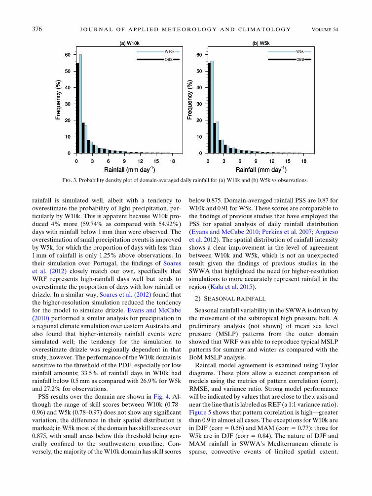
rainfall is simulated well, albeit with a tendency to
overestimate the probability of light precipitation, par-
ticularly by W10k. This is apparent because W10k pro-
duced 4% more (59.74% as compared with 54.92%)
days with rainfall below 1mm than were observed. The
overestimation of small precipitation events is improved
by W5k, for which the proportion of days with less than
1mm of rainfall is only 1.25% above observations. In
their simulation over Portugal, the findings of Soares
et al. (2012) closely match our own, specifically that
WRF represents high-rainfall days well but tends to
overestimate the proportion of days with low rainfall or
drizzle. In a similar way, Soares et al. (2012) found that
the higher-resolution simulation reduced the tendency
for the model to simulate drizzle. Evans and McCabe
(2010) performed a similar analysis for precipitation in
a regional climate simulation over eastern Australia and
also found that higher-intensity rainfall events were
simulated well; the tendency for the simulation to
overestimate drizzle was regionally dependent in that
study, however. The performance of theW10k domain is
sensitive to the threshold of the PDF, especially for low
rainfall amounts; 33.5% of rainfall days in W10k had
rainfall below 0.5mm as compared with 26.9% for W5k
and 27.2% for observations.
PSS results over the domain are shown in Fig. 4. Al-
though the range of skill scores between W10k (0.78–
0.96) and W5k (0.78–0.97) does not show any significant
variation, the difference in their spatial distribution is
marked; inW5kmost of the domain has skill scores over
0.875, with small areas below this threshold being gen-
erally confined to the southwestern coastline. Con-
versely, themajority of theW10k domain has skill scores
below 0.875. Domain-averaged rainfall PSS are 0.87 for
W10k and 0.91 forW5k. These scores are comparable to
the findings of previous studies that have employed the
PSS for spatial analysis of daily rainfall distribution
(Evans and McCabe 2010; Perkins et al. 2007; Argüesoet al. 2012). The spatial distribution of rainfall intensity
shows a clear improvement in the level of agreement
between W10k and W5k, which is not an unexpected
result given the findings of previous studies in the
SWWA that highlighted the need for higher-resolution
simulations to more accurately represent rainfall in the
region (Kala et al. 2015).
2) SEASONAL RAINFALL
Seasonal rainfall variability in the SWWA is driven by
the movement of the subtropical high pressure belt. A
preliminary analysis (not shown) of mean sea level
pressure (MSLP) patterns from the outer domain
showed that WRF was able to reproduce typical MSLP
patterns for summer and winter as compared with the
BoM MSLP analysis.
Rainfall model agreement is examined using Taylor
diagrams. These plots allow a succinct comparison of
models using the metrics of pattern correlation (corr),
RMSE, and variance ratio. Strong model performance
will be indicated by values that are close to the x axis and
near the line that is labeled as REF (a 1:1 variance ratio).
Figure 5 shows that pattern correlation is high—greater
than 0.9 in almost all cases. The exceptions forW10k are
in DJF (corr 5 0.56) and MAM (corr 5 0.77); those for
W5k are in DJF (corr 5 0.84). The nature of DJF and
MAM rainfall in SWWA’s Mediterranean climate is
sparse, convective events of limited spatial extent.
FIG. 3. Probability density plot of domain-averaged daily rainfall for (a) W10k and (b) W5k vs observations.
376 JOURNAL OF APPL IED METEOROLOGY AND CL IMATOLOGY VOLUME 54

Sparse, convective precipitation has been found by other
studies (Soares et al. 2012; Kala et al. 2015) to be difficult
for WRF to simulate well, particularly when using con-
vective parameterization, and therefore the lower cor-
relations we have seen for these two seasons are
expected. The higher-resolution W5k simulation is able
to improve performance with respect to the convective-
dominated rainfall seasons (DJF andMAM) as a result of
explicitly resolved convection and a higher-resolution
domain, which can represent the patchy nature of this
precipitation with greater skill. This is most significant in
DJF, for which period theW5k simulation has improved
W10k results from a pattern correlation of 0.55 to one of
0.84 and a variance ratio from 4.4 to 0.7. For the seasons
of JJA and SON, for which rainfall in the SWWA is
dominated by frontal systems, W5k deteriorates relative
to the performance of W10k, especially with respect to
the variance ratio, indicating that W5k is not capturing
the variability of the rainfall in JJA and SON as well as
W10k. This deterioration in JJA and SON rainfall var-
iability for W5k can be explained by the strongly nega-
tive coastal winter rainfall biases in W5k, caused by
domain-edge effects, which are discussed further in the
following paragraphs.
Rainfall seasonal bias for both W10k and W5k is
shown in Fig. 6. Across the region, and for all seasons
except JJA, bias remains low and predominantly nega-
tive. JJA rainfall biases are considerably larger than in
other seasons because most of the region’s rainfall
occurs in this season (Fig. 2c). Furthermore, the spatial
distribution of bias shows a marked difference between
W10k and W5k. W10k is producing a band of positive
rainfall bias along the west coast of the region that is not
present in the higher-resolution W5k. The area of pos-
itive bias in W10k aligns closely with the Darling Scarp,
which runs parallel to the coast at this point (as shown in
FIG. 4. PSS of daily precipitation for (a) W10k and (b) W5k.
FIG. 5. Taylor plot showing seasonal rainfall performance forW10k
(red) and W5k (blue).
FEBRUARY 2015 ANDRYS ET AL . 377

Fig. 1b). The pattern of bias is consistent with the
‘‘windward/lee effect,’’ in which mesoscale models tend
to overestimate rainfall on the windward side of topo-
graphical features, as described by Wulfmeyer et al.
(2008). In a 30-yr climate simulation over Germany,
Warrach-Sagi et al. (2013) also found evidence of the
windward/lee effect in WRF at 10-km resolution, but
this error was overcome in short-run simulations at
a convection-resolving scale (5 km). Consistent with
Warrach-Sagi et al. (2013), W5k improves the repre-
sentation of the Darling Scarp’s influence on rainfall
because W5k is able to eliminate the positive bias at the
coast and much of the strong negative bias in the area to
the east of the Darling Scarp. W5k is still showing an
overall negative bias in this region, however, which
suggests that the 5-km resolution is still not sufficient to
fully resolve the meteorological influence of this topo-
graphical feature, which is supported by findings from
Pitts and Lyons (1990) who found that representing
the wind-generated turbulence of the scarp requires a
0.5-km resolution.
While the W5k simulation is overcoming the
resolution-induced positive bias at the Darling Scarp, it
is further enhancing the negative bias in the southwest
corner of the region in JJA: up to 80mmmonth21, which
represents a relative error of approximately 60% of
rainfall. To diagnose whether this bias could have re-
sulted from grid-boundary interference, we considered
the proximity of the area in question to the edge of the
W5k grid. The southwest corner of the SWWA landmass
begins 20 km (4 grid points) from the western boundary
of the domain. A 10-gridpoint relaxation zone has been
removed from this domain, but at 5-km resolution this
represents a relaxation zone of only 50 km. It is there-
fore possible that this region is experiencing some
anomalous rainfall output as a consequence of edge ef-
fects in this area interfering with the response of the
model, as was found in Lowrey and Yang (2008) and
Seth and Giorgi (1998).
A simulation (called W5k-ext) was run for the JJA
period of 2007 (plus a 3-month spinup) with a 5-km
domain extended to the south and west by 10 grid points
to allow for further enhanced development of the frontal
processes in this region away from the edge effects of the
domain. This run was compared with a simulation ini-
tialized at the same time but using the standard 5-km
FIG. 6. Average seasonal rainfall bias (observation 2 simulation) for (a) W10k and (b) W5k.
378 JOURNAL OF APPL IED METEOROLOGY AND CL IMATOLOGY VOLUME 54
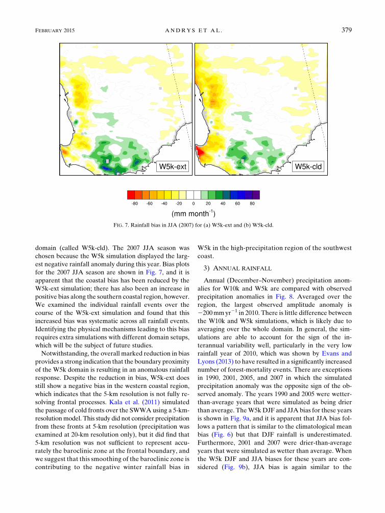
domain (called W5k-cld). The 2007 JJA season was
chosen because the W5k simulation displayed the larg-
est negative rainfall anomaly during this year. Bias plots
for the 2007 JJA season are shown in Fig. 7, and it is
apparent that the coastal bias has been reduced by the
W5k-ext simulation; there has also been an increase in
positive bias along the southern coastal region, however.
We examined the individual rainfall events over the
course of the W5k-ext simulation and found that this
increased bias was systematic across all rainfall events.
Identifying the physical mechanisms leading to this bias
requires extra simulations with different domain setups,
which will be the subject of future studies.
Notwithstanding, the overall marked reduction in bias
provides a strong indication that the boundary proximity
of the W5k domain is resulting in an anomalous rainfall
response. Despite the reduction in bias, W5k-ext does
still show a negative bias in the western coastal region,
which indicates that the 5-km resolution is not fully re-
solving frontal processes. Kala et al. (2011) simulated
the passage of cold fronts over the SWWAusing a 5-km-
resolutionmodel. This study did not consider precipitation
from these fronts at 5-km resolution (precipitation was
examined at 20-km resolution only), but it did find that
5-km resolution was not sufficient to represent accu-
rately the baroclinic zone at the frontal boundary, and
we suggest that this smoothing of the baroclinic zone is
contributing to the negative winter rainfall bias in
W5k in the high-precipitation region of the southwest
coast.
3) ANNUAL RAINFALL
Annual (December–November) precipitation anom-
alies for W10k and W5k are compared with observed
precipitation anomalies in Fig. 8. Averaged over the
region, the largest observed amplitude anomaly is
2200mmyr21 in 2010. There is little difference between
the W10k and W5k simulations, which is likely due to
averaging over the whole domain. In general, the sim-
ulations are able to account for the sign of the in-
terannual variability well, particularly in the very low
rainfall year of 2010, which was shown by Evans and
Lyons (2013) to have resulted in a significantly increased
number of forest-mortality events. There are exceptions
in 1990, 2001, 2005, and 2007 in which the simulated
precipitation anomaly was the opposite sign of the ob-
served anomaly. The years 1990 and 2005 were wetter-
than-average years that were simulated as being drier
than average. TheW5kDJF and JJA bias for these years
is shown in Fig. 9a, and it is apparent that JJA bias fol-
lows a pattern that is similar to the climatological mean
bias (Fig. 6) but that DJF rainfall is underestimated.
Furthermore, 2001 and 2007 were drier-than-average
years that were simulated as wetter than average. When
the W5k DJF and JJA biases for these years are con-
sidered (Fig. 9b), JJA bias is again similar to the
FIG. 7. Rainfall bias in JJA (2007) for (a) W5k-ext and (b) W5k-cld.
FEBRUARY 2015 ANDRYS ET AL . 379

climatological mean, whereas DJF shows a very strong
positive bias (W10k simulation bias is not shown be-
cause the pattern of bias closely matches that of W5k).
This result indicates that simulation limitations with
respect to dry-season rainfall events are the cause of the
model’s inability to detect the sign of the rainfall
anomaly in these years.
To establish the source of the dry-season rainfall er-
ror, we considered the region’s dry-season climatologi-
cal behavior. Dry-season rainfall tends to be sporadic
and sparse, but regional-scale rainfall events take place
every 3–4 years on average. These events, triggered by
high-level moisture advection from the tropics via me-
ridional troughs, are simulated poorly by the model.
Over the course of our simulation, 9 of these dry-season
regional-scale rainfall events were observed. Our model
generated 11 such events, 4 of which coincided with
observed precipitation events in 2000, 2001, 2007, and
2008. Rainfall was overestimated for these events in
both 2001 and 2007, leading to the anomalously high
simulated mean rainfall in these years. Observed DJF
rainfall in 1990 was also high as a result of a regional-
scale rainfall event; this particular event was poorly
simulated, however. The relatively low DJF bias seen in
Fig. 6 shows that, over the 30-yr climatological period,
the model is accounting for the extent of these regional-
scale rainfall events well. When individual events are
considered, however, the timing and magnitude are not
well represented. We conducted a number of short
simulations during 2007 with different initialization
dates and found that the moisture-advection processes
are particularly sensitive to the time since initialization,
but there was no consistent pattern in this behavior.
Further research is required to fully understand the
nature of the misrepresentation of moisture advection
within the outer domain of our model.
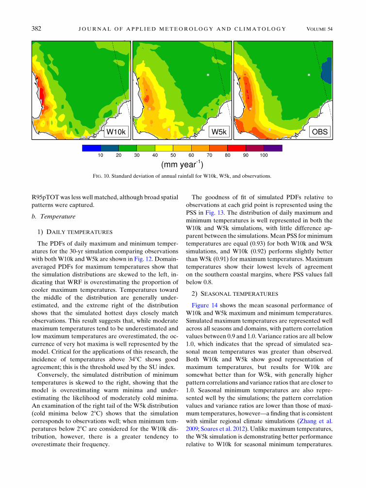
Figure 10 shows the spatial distribution of the stan-
dard deviation for annual rainfall. As expected, the
largest observed variability is found in the highest-
rainfall regions. Both W10k and W5k are able to rep-
resent the magnitude of the standard-deviation changes
throughout the domain well. W5k is able to account for
the spatial distribution of standard deviations better
than W10k is in the midwest coastal region, but there is
a large disparity between observations and W5k in the
southwestern corner of the landmass that can be at-
tributed to the grid-edge effects that are enhancing
negative bias in this region.
4) EXTREME INDICES
We next examine indices that consider the contribu-
tion of rainfall from high-intensity events (R95pTOT
and RX5day) and average rainfall intensity (SDII).
From observations of SDII shown in Fig. 11a, it is ap-
parent that the most intense rainfall is inland of the west
coast, to the east of the Darling Scarp. W5k shows good
spatial agreement with observations, especially in the
area of highest precipitation intensity. SDII is under-
estimated by W5k in the southwest corner by approxi-
mately 2mmday21. W10k represents the SDII as being
the highest along the west coast, whereas the observa-
tions show that the highest-intensity rainfall occurs to
the east of the Darling Scarp. The W10k representation
of SDII is lacking in the finescale spatial structure of this
index, which is well developed in W5k. W10k does,
however, provide a better representation in the south-
west corner and the interior of the domain than W5k
does.
The RX5day index measures the highest annual
rainfall in a 5-day period. Climatologically averaged
annual RX5day is shown in Fig. 11b for the observations
and for the W10k and W5K simulations. Similar to the
SDII index, observations show that RX5day is highest in
the region east of the Darling Scarp and along the
southern coast, with declining intensity inland. Al-
though there is spatial agreement for the W5k simula-
tion, it is less well represented than the average intensity
that was identified by the SDII index (Fig. 11). W10k
does not capture the spatial pattern of Rx5day on the
coast or in the Darling Scarp, and both W10k and W5k
are overestimating RX5day in the interior.
The contribution of rainfall from the highest-intensity
rainfall events (above the 95th percentile) is measured
by the R95pTOT index. This metric differs fromRx5day
because it considers all of the high-intensity rainfall
events in a year over the percentile threshold whereas
the RX5day only represents a single high-intensity event
from each year. Observations for the R95pTOT index
show a clear gradient from the southwest corner to the
FIG. 8. Time series (1981–2010) of domain-averaged annual
rainfall anomaly for observations (solid blue), W10k (dotted red),
and W5k (solid red).
380 JOURNAL OF APPL IED METEOROLOGY AND CL IMATOLOGY VOLUME 54

northeast of the domain that is not as well defined in the
W10k and W5k simulations (Fig. 11c). Both simulations
show a significant departure from observations in the
southwest corner, where the model is underestimating
this index by over 100mm (50%) in W5k and 50mm
(25%) inW10k. TheW10k domain continues tomiss the
spatial distribution of the rainfall on the west coast; both
W10k and W5k represent R95pTOT well over the in-
terior of the SWWA, however. The RX5day and
R95pTOT indices were evaluated by Argüeso et al.(2012) in a regional climate simulation over Spain. Their
assessment of the performance of these metrics mirrors
what we found here: the Rx5day index was well repre-
sented both spatially and with respect to magnitude and
FIG. 9. Mean W5k (left) DJF and (right) JJA rainfall bias for (a) 1990 and 2005 and (b) 2001 and 2007.
FEBRUARY 2015 ANDRYS ET AL . 381
R95pTOTwas less well matched, although broad spatial
patterns were captured.
b. Temperature
1) DAILY TEMPERATURES
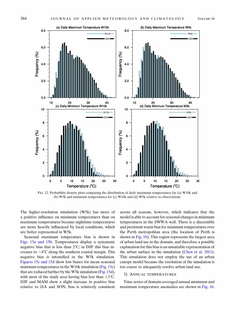
The PDFs of daily maximum and minimum temper-
atures for the 30-yr simulation comparing observations
with bothW10k andW5k are shown in Fig. 12. Domain-
averaged PDFs for maximum temperatures show that
the simulation distributions are skewed to the left, in-
dicating that WRF is overestimating the proportion of
cooler maximum temperatures. Temperatures toward
the middle of the distribution are generally under-
estimated, and the extreme right of the distribution
shows that the simulated hottest days closely match
observations. This result suggests that, while moderate
maximum temperatures tend to be underestimated and
low maximum temperatures are overestimated, the oc-
currence of very hot maxima is well represented by the
model. Critical for the applications of this research, the
incidence of temperatures above 348C shows good
agreement; this is the threshold used by the SU index.
Conversely, the simulated distribution of minimum
temperatures is skewed to the right, showing that the
model is overestimating warm minima and under-
estimating the likelihood of moderately cold minima.
An examination of the right tail of the W5k distribution
(cold minima below 28C) shows that the simulation
corresponds to observations well; when minimum tem-
peratures below 28C are considered for the W10k dis-
tribution, however, there is a greater tendency to
overestimate their frequency.
The goodness of fit of simulated PDFs relative to
observations at each grid point is represented using the
PSS in Fig. 13. The distribution of daily maximum and
minimum temperatures is well represented in both the
W10k and W5k simulations, with little difference ap-
parent between the simulations.Mean PSS forminimum
temperatures are equal (0.93) for both W10k and W5k
simulations, and W10k (0.92) performs slightly better
than W5k (0.91) for maximum temperatures. Maximum
temperatures show their lowest levels of agreement
on the southern coastal margins, where PSS values fall
below 0.8.
2) SEASONAL TEMPERATURES
Figure 14 shows the mean seasonal performance of
W10k and W5k maximum and minimum temperatures.
Simulated maximum temperatures are represented well
across all seasons and domains, with pattern correlation
values between 0.9 and 1.0. Variance ratios are all below
1.0, which indicates that the spread of simulated sea-
sonal mean temperatures was greater than observed.
Both W10k and W5k show good representation of
maximum temperatures, but results for W10k are
somewhat better than for W5k, with generally higher
pattern correlations and variance ratios that are closer to
1.0. Seasonal minimum temperatures are also repre-
sented well by the simulations; the pattern correlation
values and variance ratios are lower than those of maxi-
mum temperatures, however—a finding that is consistent
with similar regional climate simulations (Zhang et al.
2009; Soares et al. 2012). Unlike maximum temperatures,
the W5k simulation is demonstrating better performance
relative to W10k for seasonal minimum temperatures.
FIG. 10. Standard deviation of annual rainfall for W10k, W5k, and observations.
382 JOURNAL OF APPL IED METEOROLOGY AND CL IMATOLOGY VOLUME 54

FIG. 11. Average values of annual precipitation indices (a) SDII, (b) RX5day, and (c) R95pTOT for W10k, W5k, and observations.
FEBRUARY 2015 ANDRYS ET AL . 383
The higher-resolution simulation (W5k) has more of
a positive influence on minimum temperatures than on
maximum temperatures because nighttime temperatures
are more heavily influenced by local conditions, which
are better represented in W5k.
Seasonal maximum temperature bias is shown in
Figs. 15a and 15b. Temperatures display a systematic
negative bias that is less than 28C; in DJF this bias in-
creases to 248C along the southern coastal margin. This
negative bias is intensified in the W5k simulation.
Figures 15c and 15d show low biases for mean seasonal
minimum temperatures in theW10k simulation (Fig. 15c)
that are reduced further by theW5k simulation (Fig. 15d),
with most of the study area having bias less than 618C.DJF and MAM show a slight increase in positive bias
relative to JJA and SON; bias is relatively consistent
across all seasons, however, which indicates that the
model is able to account for seasonal changes inminimum
temperatures in the SWWA well. There is a discernible
and persistent warm bias forminimum temperatures over
the Perth metropolitan area (the location of Perth is
shown in Fig. 1b). This region represents the largest area
of urban land use in the domain, and therefore a possible
explanation for this bias is an unsuitable representation of
the urban surface in the simulation (Chen et al. 2011).
This simulation does not employ the use of an urban
canopy model because the resolution of the simulation is
too coarse to adequately resolve urban land use.
3) ANNUAL TEMPERATURES
Time series of domain-averaged annual minimum and
maximum temperature anomalies are shown in Fig. 16.
FIG. 12. Probability density plots comparing the distribution of daily maximum temperatures for (a) W10k and
(b) W5k and minimum temperatures for (c) W10k and (d) W5k relative to observations.
384 JOURNAL OF APPL IED METEOROLOGY AND CL IMATOLOGY VOLUME 54

Over the duration of the simulation, observed temper-
ature anomalies are small, less than 618C. These plots
demonstrate that the simulations are able to reflect the
interannual variations in temperature that are seen at
the domain scale. This is especially true of minimum
temperatures, for which the simulated anomalies are
close to the observations. Simulated maximum temper-
atures show less skill in accounting for the observed
variability. Although the magnitudes of the anomalies
are well simulated over the 30-yr period, in 1984, 1987,
1998, 2001, 2003, and 2009 the sign of the temperature
anomaly is poorly represented. The years 1984 and
1987 were colder-than-average years that were simu-
lated as warmer than average. Conversely, 1998, 2001,
2003, and 2009 were warmer-than-average years but
were simulated as colder than average. It was found
FIG. 13. PSS of (a) maximum temperature distributions and (b) minimum temperature distributions for (left) W10k
and (right) W5k.
FEBRUARY 2015 ANDRYS ET AL . 385

that, similar to annual rainfall anomalies, these maxi-
mum temperature anomalies arise from fluctuations in
the warm-season (DJF) biases, whereas the cooler-
season (JJA) biases remain constant throughout the
simulation. We considered whether these anomalous
summer maximum temperature biases were linked
with the model’s poor simulation of regional-scale DJF
rain events and could not find a consistent relationship
with rainfall.
4) EXTREME INDICES
The FD index provides an annual count of days on
which minimum temperatures are below 28C. The cli-
matologically averaged count of FD across the domain
for W10k, W5k, and observations is shown in Fig. 17a.
Observations highlight that the areas with the most FD
are concentrated in the interior of the region and ap-
proximately 100km inland of the western coastal mar-
gin. W10k andW5k show that the spatial extent of FD is
represented well around the coastal regions. BothW10k
and W5k overestimate the frost risk in the area to the
east of the Darling Scarp and in the northwest corner of
the domain, and FD is underestimated in the northeast.
The higher-resolution W5k demonstrates a reduction in
positive bias when compared with W10k. This im-
provement is enabled by the higher-resolution simula-
tion allowing for more accurate representation of the
local conditions, such as topography, that contribute to
frost conditions.
Figure 17b illustrates the SU index. The simulated
spatial representation of this index is overall satisfactory,
and there is little difference between the two domains.
This result is consistent with other studies that also
found that maximum temperatures do not tend to be as
heavily influenced as minimum temperatures are by
increases in model resolution (Soares et al. 2012).
There is an underestimation of the incidence of SU
days in the north of the domain by approximately 5–10
days per year, which is a result of the negative bias in
maximum temperatures that was found in the region
(shown in Fig. 15).
The temporal characteristics of these temperature
thresholds are very important, particularly how they
interact with the cereal-crop growing season. As such,
the mean monthly counts of these indices are now con-
sidered. Figure 18 shows that W10k and W5k are both
able to represent the spatiotemporal development of FD
in the growing season, with W5k showing an improved
spatial representation and a reduction in positive bias.
Simulations are demonstrating a small negative bias for
early-season frost days (in May and June), showing that
the model develops frost conditions later than observed;
the spatiotemporal representation of frost is satisfac-
tory, however.
Because the growing season is over the austral win-
ter, the high-temperature threshold SU is exceeded
less in the growing season than is FD. Figure 19 shows
the monthly distribution of SU in those months that
experience SU and highlights that the likelihood of SU
in the growing season is low, with the north of the re-
gion experiencing less than 2 SU in October. Both
W10k and W5k underestimate the extent of SU, but
FIG. 14. Taylor plots showing the relative skill of W10k and W5k simulations for seasonal (a) maximum and (b) minimum temperatures.
386 JOURNAL OF APPL IED METEOROLOGY AND CL IMATOLOGY VOLUME 54

FIG. 15. Average seasonal temperature bias (observation 2 simulation) for (a) W10k maximum temperature, (b) W5k maximum
temperature, (c) W10k minimum temperature, and (d) W5k minimum temperature.
FEBRUARY 2015 ANDRYS ET AL . 387

both simulations are able to account for the spatial
distribution of monthly SU days, with W5k providing
an improved representation of their magnitude rela-
tive to W10k.
4. Discussion and conclusions
We present an evaluation of the RCM WRF over
the SWWA for 30 years between 1981 and 2010 to ex-
amine the ability of the model to accurately represent
the ‘‘climatology’’ of the region, including the clima-
tology of extreme events. Our study compared two do-
main resolutions: 10-km resolution using convective
parameterization (W10k) and a 5-km domain that re-
solves convection explicitly (W5k).
Overall, we found that the simulation performed well in
representing the climatology of the region. The statistical
distribution of daily temperatures and rainfall showed
that, while WRF tended to underestimate average maxi-
mum temperatures, warm extremes were well repre-
sented. This pattern was followed by rainfall, where daily
high-intensity rainfall events were simulated well, and was
mirrored by minimum temperatures, for which the mean
was overestimated but very cold days showed good
agreement with observations.
An analysis of seasonal variation showed that WRF
was able to model seasonal minimum and maximum
temperatures well. The W5k simulation improved the
representation of minimum temperatures because of the
improved resolution of local topographical effects but
introduced additional bias for maximum temperatures.
There were some large biases associated with JJA pre-
cipitation. While the positive bias on the midwest coast
was overcome by W5k because of an improved topo-
graphical resolution of the Darling Scarp, the negative
bias in the southwest corner was further enhanced. Bias
in this region was influenced by the proximity of the grid
edge to the coast in theW5k domain. This is indicated by
a 3-month simulation for JJA in 2007 that showed that
more than 50% of this bias was removed by expanding
the W5k domain in a southerly and westerly direction.
Even with the edge effects eliminated in the W5k-
extended domain, a small negative bias on the south-
west coast persisted. This follows the results from other
studies in the SWWA that found that a 5-km resolution
is not sufficient to fully resolve the baroclinic zone of the
frontal systems that bring most of the JJA rainfall to the
region (Kala et al. 2011). The W5k simulation was able
to demonstrate significant improvements in the repre-
sentation of DJF and MAM rainfall. Because of the
edge effects that affect this simulation, it is not recom-
mended that this domain be used for examining coastal
precipitation, however. For future regional climate
simulations it is strongly recommended that a larger do-
main, allowing for greater distance from the grid bound-
ary to the coast, be used. The optimal spatial extent and
positioning of the high-resolution domain relative to the
coast is currently unknown, and further simulationswill be
required to establish how frontal rainfall processes are
influenced by the location of the domain, as well as by
horizontal and vertical resolution.
Extreme temperature indices were simulated well by
WRF, especially by W5k, which was able to represent
not only the magnitude but also the spatial and temporal
distribution of FD and SU. Precipitation indices SDII,
Rx5day, and R95pTOT were also modeled satisfacto-
rily, but their performance was influenced by the biases
found in both the W10k and W5k simulations. Soares
et al. (2012) found that higher-resolution domains im-
proved the simulation of precipitation extremes, and our
results are not as conclusive in this respect. Note, how-
ever, that the Soares et al. (2012) highest-resolution
domain was 9 km and used convective parameteriza-
tion, comparable to ourW10k domain. Furthermore, the
FIG. 16. Time series (1981–2010) of domain-averaged annual (a) maximum and (b) minimum temperature anomaly
for observations (solid blue), W10k (dotted red), and W5k (solid red).
388 JOURNAL OF APPL IED METEOROLOGY AND CL IMATOLOGY VOLUME 54

downscaling ratio between the two domains compared
in Soares et al. (2012) was 3, whereas the downscaling
ratio used in our research was 2.
It was expected that the W5k simulation would
demonstrate improved results when compared with
W10k, but this finding was equivocal. W5k is influ-
enced by edge effects in the southwestern coastal
regions but even removing these affected areas from
our analysis does not always elevate the performance
of the W5k simulation above that of W10k. For ex-
ample, W10k provided a better representation of
R95pTOT and SDII relative to W5k in the interior
of the domain. Despite the fact that the performance
of W5k is not always superior to W10k, this high-
resolution model does consistently demonstrate im-
proved simulation skill with respect to convective
precipitation, rainfall surrounding the Darling Scarp,
and also frost.
For applications related to cereal-crop produc-
tion in SWWA, the W5k simulation is useful because it
reduces the negative JJA rainfall bias in the interior
of the domain, which is the area of main agricultural
production in the region. Furthermore, representa-
tion of the daily distribution of precipitation is improved
significantly by the higher-resolution simulation, which
indicates that the W5k simulation is providing a better
FIG. 17. Values of the temperature indices (a) FD and (b) SU for W10k, W5k, and observations.
FEBRUARY 2015 ANDRYS ET AL . 389

spatial representation of rainfall. W5k does not show as
marked an improvement on temperature representa-
tion, and this result is because temperatures, particularly
maxima, are not as heavily affected by the finer-scale
features that the higher-resolution domain improves
upon. When we consider the temporal distributions of
the SU and FD indices in accordance with the growing
season, however, we do see that, for both metrics, W5k
improves the spatiotemporal representation of these
indices relative to W10k.
There are a number of regional climate studies that
demonstrate improved simulation performance when
comparing domains of 30–50 km with domains of 9–
15 km in which both domains employ convective pa-
rameterization (Cardoso et al. 2013; Soares et al. 2012;
Heikkilä et al. 2011). Fewer studies compare a 10-km
domain with a higher-resolution grid that is explicitly
resolving convection. Villarroel et al. (2013) found
that a high-resolution 5-km domain over southern
Chile improved model performance for both temper-
ature and precipitation relative to the driving data, and
this result was attributed to improved topographical
resolution, but the domain was not compared with
a lower-resolution WRF grid. In a simulation over
central Japan, Kusaka et al. (2010) found that 4-km
resolution represented a 5-yr climatology well; again,
these results were compared with a lower-resolution
WRF grid. Warrach-Sagi et al. (2013) conducted a 30-yr
simulation over Germany at 10-km resolution and then
compared these results with a shorter, convection-
resolving simulation at 5-km resolution. Their findings
were consistent with our own in demonstrating that
a convection-resolving resolution can overcome the
windward/lee effect that is apparent at 10-km resolution
(W10k), and they support the use of high-resolution,
convection-resolving simulations for RCM.
On the basis of the results of W10k and W5k, partic-
ularly the spatial and temporal representation of the
climate extremes that were considered in this research,
we have high confidence in the model for regional cli-
mate simulations over SWWA.
Acknowledgments. This research was supported by
an Australian Grains Research and Development
FIG. 18. Monthly (05–10 5 May–October) values of FD over the growing season for (a) W10k, (b) W5k, and (c) observations.
390 JOURNAL OF APPL IED METEOROLOGY AND CL IMATOLOGY VOLUME 54

FIG. 19. Monthly (01–04 5 January–April; 10–12 5 October–December) values of SU for (a) W10k,
(b) W5k, and (c) observations.
FEBRUARY 2015 ANDRYS ET AL . 391

Corporation (GRDC)Grant (MCV0013). Julia Andrys
is supported by an Australian Postgraduate Award and
a GRDC Top Up Scholarship. Jatin Kala is supported
by the Australian Research Council Centre of Excel-
lence for Climate Systems Science (CE110001028). The
research group led by Associate Professor Jason Evans
at the University of New South Wales, Australia, pro-
vided the modified version of WRFv3.3 used in this
study and assisted in the preprocessing of the input
data. Computational modeling was supported by iVEC
through the use of advanced computing resources
provided by the Pawsey Super Computing Centre lo-
cated at iVec@Murdoch. It was funded under the Na-
tional ComputationalMerit Allocation Scheme and the
iVec Partner Allocation Scheme. All of this support is
gratefully acknowledged. The authors also thank the
two anonymous reviewers whose comments helped to
improve this manuscript.
REFERENCES
Allen, C. D., and Coauthors, 2010: A global overview of drought
and heat-induced tree mortality reveals emerging climate
change risks for forests. For. Ecol. Manage., 259, 660–684,
doi:10.1016/j.foreco.2009.09.001.
Argüeso, D., J. M. Hidalgo-Muñoz, S. R. Gámiz-Fortis, M. J.
Esteban-Parra, J. Dudhia, and Y. Castro-Díez, 2011: Evalua-tion of WRF parameterizations for climate studies over
southern Spain using a multistep regionalization. J. Climate,
24, 5633–5651, doi:10.1175/JCLI-D-11-00073.1.
——, ——, ——, ——, and Y. Castro-Díez, 2012: Evaluation of
WRF mean and extreme precipitation over Spain: Present
climate (1970–99). J. Climate, 25, 4883–4897, doi:10.1175/
JCLI-D-11-00276.1.
Asseng, S., I. Foster, and N. C. Turnder, 2011: The impact of
temperature variability on wheat yields.Global Change Biol.,
17, 997–1012, doi:10.1111/j.1365-2486.2010.02262.x.——, D. Thomas, P. McIntosh, O. Alves, and N. Khimashia, 2012:
Managing mixed wheat–sheep farms with a seasonal forecast.
Agric. Syst., 113, 50–56, doi:10.1016/j.agsy.2012.08.001.
Brouwers, N. C., J. Mercer, T. Lyons, P. Poot, E. Veneklaas, andG.
Hardy, 2012: Climate and landscape drivers of tree decline in
a Mediterranean ecoregion. Ecol. Evol., 3, 67–79, doi:10.1002/
ece3.437.
Cardoso, R. M., P. M. M. Soares, P. M. A. Miranda, and
M. BeloPereira, 2013: WRF high resolution simulation of
Iberian mean and extreme precipitation climate. Int. J.
Climatol., 33, 2591–2608, doi:10.1002/joc.3616.
Chen, F., and J. Dudhia, 2001: Coupling an advanced land surface–
hydrology model with the Penn State–NCAR MM5 modeling
system. Part I: Model implementation and sensitivity. Mon.
Wea. Rev., 129, 569–585, doi:10.1175/1520-0493(2001)129,0569:
CAALSH.2.0.CO;2.
——, and Coauthors, 2011: The integrated WRF/urban modelling
system: Development, evaluation, and applications to urban en-
vironmental problems. Int. J. Climatol., 31, 273–288, doi:10.1002/
joc.2158.
Chotamonsak, C., E. P. Salathé Jr., J. Kreasuwan, S. Chantara, and
K. Siriwitayakorn, 2011: Projected climate change over
Southeast Asia simulated using aWRF regional climate model.
Atmos. Sci. Lett., 12, 213–219, doi:10.1002/asl.313.
Christensen, J.H., T.R.Carter,M.Rummukainen, andG.Amanatidis,
2007: Evaluating the performance and utility of regional climate
models: The PRUDENCE project. Climatic Change, 81, 1–6,
doi:10.1007/s10584-006-9211-6.
Chu, J., K.Warrach-Sagi,V.Wulfmeyer, T. Schwitalla, andH.Bauer,
2010: Regional climate simulation (1989-2009) with WRF in
the CORDEX-Europe domain. Abstracts, 10th EMS Annual
Meeting and 8th European Conf. on Applied Climatology
(ECAC), Zürich, Switzerland, European Meteorological Soci-ety, EMS2010-209. [Available online at http://meetingorganizer.
copernicus.org/EMS2010/EMS2010-209-1.pdf.]
Clifford, M. J., P. D. Royer, N. S. Cobb, D. D. Breshears, and P. L.
Ford, 2013: Precipitation thresholds and drought-induced tree
die-off: Insights from patterns of Pinus edulis mortality along
an environmental stress gradient. New Phytol., 200, 413–421,
doi:10.1111/nph.12362.
Dee, D. P., and Coauthors, 2011: The ERA-Interim reanalysis:
Configuration and performance of the data assimilation system.
Quart. J. Roy. Meteor. Soc., 137, 553–597, doi:10.1002/qj.828.
Donat, M. G., G. C. Leckebusch, J. G. Pinto, and U. Ulbrich, 2010:
European storminess and associated circulation weather
types: Future changes deduced from a multi-model ensemble
of GCM simulations. Climate Res., 42, 27–43, doi:10.3354/
cr00853.
Dudhia, J., 1989: Numerical study of convection observed during
the Winter Monsoon Experiment using a mesoscale two-
dimensional model. J. Atmos. Sci., 46, 3077–3107, doi:10.1175/
1520-0469(1989)046,3077:NSOCOD.2.0.CO;2.
Easterling, D. R., G. A. Meehl, C. Parmesan, S. A. Changnon, T. R.
Karl, and L. O. Mearns, 2000: Climate extremes: Observations,
modeling, and impacts. Science, 289, 2068–2074, doi:10.1126/
science.289.5487.2068.
Ekström, M., H. J. Fowler, C. G. Kilsby, and P. D. Jones, 2005: New
estimates of future changes in extreme rainfall across the UK
using regional climate model integrations. 2. Future estimates
and use in impact studies. J. Hydrol., 300, 234–251, doi:10.1016/
j.jhydrol.2004.06.019.
England, M. H., C. C. Ummenhofer, and A. Santoso, 2006: In-
terannual rainfall extremes over southwest Western Australia
linked to Indian Ocean climate variability. J. Climate, 19,
1948–1969, doi:10.1175/JCLI3700.1.
Evans, B., and T. Lyons, 2013: Bioclimatic extremes drive forest
mortality in southwest, Western Australia. Climate, 1 (2), 28–
52, doi:10.3390/cli1020028.
Evans, J. P., and M. F. McCabe, 2010: Regional climate simulation
over Australia’s Murray-Darling basin: A multitemporal as-
sessment. J. Geophys. Res., 115, D14114, doi:10.1029/
2010JD013816.
——, M. Ekström, and F. Ji, 2012: Evaluating the performance of
a WRF physics ensemble over south-east Australia. Climate
Dyn., 39, 1241–1258, doi:10.1007/s00382-011-1244-5.
Fitzpatrick, M. C., A. D. Gove, N. J. Sanders, and R. R. Dunn,
2008: Climate change, plant migration, and range collapse in
a global biodiversity hotspot: The Banksia (Proteaceae) of
Western Australia. Global Change Biol., 14, 1337–1352,
doi:10.1111/j.1365-2486.2008.01559.x.
Fowler, H. J., M. Ekström, C. G. Kilsby, and P. D. Jones, 2005: New
estimates of future changes in extreme rainfall across the UK
using regional climate model integrations. 1. Assessment of
control climate. J. Hydrol., 300, 212–233, doi:10.1016/
j.jhydrol.2004.06.017.
392 JOURNAL OF APPL IED METEOROLOGY AND CL IMATOLOGY VOLUME 54
Gao, Y., J. S. Fu, J. B. Drake, Y. Liu, and J. F. Lamarque, 2012:
Projected changes of extreme weather events in the eastern
United States based on a high resolution climate model-
ing system. Environ. Res. Lett., 7, 044025, doi:10.1088/
1748-9326/7/4/044025.
Gentilli, J., 1971: Climates of Australia and New Zealand. Elsevier,
405 pp.
Giorgi, F., C. Jones, and G. R. Asrar, 2009: Addressing climate
information needs at the regional level: The CORDEX
framework. WMO Bull., 58, 175–183. [Available online at
https://www.wmo.int/pages/publications/bulletin_en/archive/
58_3_en/documents/58_3_giorgi_en.pdf.]
Grell, G. A., S. Emeis, W. R. Stockwell, T. Schoenemeyer,
R. Forkel, J. Michalakes, R. Knoche, and W. Seidl, 2000:
Application of a multiscale, coupled MM5/chemistry
model to the complex terrain of the VOTALP valley
campaign. Atmos. Environ., 34, 1435–1453, doi:10.1016/
S1352-2310(99)00402-1.
Heikkilä, U., A. Sandvik, and A. Sorteberg, 2011: Dynamical down-
scaling of ERA-40 in complex terrain using theWRF regional
climate model. Climate Dyn., 37, 1551–1564, doi:10.1007/
s00382-010-0928-6.
Hong, S.-Y., and J.-O. J. Lim, 2006: The WRF single-moment
6-class microphysics scheme (WSM6). J. Korean Meteor. Soc.,
42, 129–151.——, J. Dudhia, and S.-H. Chen, 2004: A revised approach to ice
microphysical processes for the bulk parameterization of
clouds and precipitation. Mon. Wea. Rev., 132, 103–120,
doi:10.1175/1520-0493(2004)132,0103:ARATIM.2.0.CO;2.
Hughes, L., 2003: Climate change and Australia: Trends, pro-
jections and impacts. Austral Ecol., 28, 423–443, doi:10.1046/
j.1442-9993.2003.01300.x.
Jones, D. A., W. Wang, and R. Fawcett, 2009: High-quality spatial
climate data-sets for Australia.Aust. Meteor. Oceanogr. J., 58,
233–248.
Kain, J. S., 2004: The Kain–Fritsch convective parameteriza-
tion: An update. J. Appl. Meteor., 43, 170–181, doi:10.1175/
1520-0450(2004)043,0170:TKCPAU.2.0.CO;2.
Kala, J., T. J. Lyons, I. J. Foster, and U. S. Nair, 2009: Validation of
a simple steady-state forecast of minimum nocturnal temper-
atures. J. Appl. Meteor. Climatol., 48, 624–633, doi:10.1175/
2008JAMC1956.1.
——, ——, and U. S. Nair, 2011: Numerical simulations of the im-
pacts of land-cover change on cold fronts in south-westWestern
Australia. Bound.-Layer Meteor., 138, 121–138, doi:10.1007/
s10546-010-9547-3.
——, J. Andrys, T. J. Lyons, I. J. Foster, and B. Evans, 2015:
Sensitivity of WRF to driving data and physics options on
a seasonal time-scale for the southwest of Western Australia.
Climate Dyn., doi:10.1007/s00382-014-2160-2, in press.
Keeling, C. D., S. C. Piper, R. B. Bacastow, M. Wahlen, T. P.
Whorf, M. Heimann, and H. A. Meijer, 2001: Exchanges
of atmospheric CO2 and13CO2 with the terrestrial biosphere and
oceans from1978 to 2000. I.Global aspects. SIOReference Series
Tech. Rep. 01-06, 28 pp. [Available online at http://scrippsco2.
ucsd.edu/publications/keeling_sio_ref_series_exchanges_of_co2_
ref_no_01-06_2001.pdf.]
King, A. D., L. V. Alexander, and M. G. Donat, 2013: The efficacy
of using gridded data to examine extreme rainfall character-
istics: A case study for Australia. Int. J. Climatol., 33, 2376–
2387, doi:10.1002/joc.3588.
Kingwell, R., 2006: Climate change in Australia: Agricultural im-
pacts and adaptation. Austr. Agribus. Rev., 14, Paper 1, 29 pp.
[Available online at http://www.agrifood.info/review/2006/
Kingwell.pdf.]
Kusaka, H., T. Takata, and Y. Takane, 2010: Reproducibility of
regional climate in central Japan using the 4-km resolution
WRF Model. SOLA, 6, 113–116, doi:10.2151/sola.2010-029.
Lowrey,M. R. K., and Z.-L. Yang, 2008: Assessing the capability of
a regional-scale weather model to simulate extreme pre-
cipitation patterns and flooding in central Texas. Wea. Fore-
casting, 23, 1102–1126, doi:10.1175/2008WAF2006082.1.
Ludwig, F., and S. Asseng, 2006: Climate change impacts on wheat
production in a Mediterranean environment in Western Aus-
tralia. Agric. Syst., 90, 159–179, doi:10.1016/j.agsy.2005.12.002.
Malcolm, J. R., C. Liu, R. P. Neilson, L. Hansen, and L. E. E.
Hannah, 2006: Global warming and extinctions of endemic
species from biodiversity hotspots.Conserv. Biol., 20, 538–548,
doi:10.1111/j.1523-1739.2006.00364.x.
Mearns, L. O., W. Gutowski, R. Jones, R. Leung, S. McGinnis,
A. Nunes, and Y. Qian, 2009: A regional climate change as-
sessment program for North America. Eos, Trans. Amer. Geo-
phys. Union, 90 (36), 311–312, doi:10.1029/2009EO360002.
Mishra, V., F. Dominguez, and D. P. Lettenmaier, 2012: Urban pre-
cipitation extremes: How reliable are regional climate models?
Geophys. Res. Lett., 39, L03407, doi:10.1029/2011GL050658.
Mlawer, E. J., S. J. Taubman, P. D. Brown, M. J. Iacono, and S. A.
Clough, 1997: Radiative transfer for inhomogeneous atmo-
spheres:RRTM, a validated correlated-kmodel for the longwave.
J. Geophys. Res., 102, 16 663–16 682, doi:10.1029/97JD00237.
Niu, S., Y. Luo, D. Li, S. Cao, J. Xia, J. Li, andM.D. Smith, 2014: Plant
growth and mortality under climatic extremes: An overview. En-
viron. Exp. Bot., 98, 13–19, doi:10.1016/j.envexpbot.2013.10.004.
Patricola, C. M., and K. H. Cook, 2013: Mid-twenty-first century
warm season climate change in the centralUnited States. Part I:
Regional and global model predictions. Climate Dyn., 40, 551–
568, doi:10.1007/s00382-012-1605-8.
Patz, J. A., D. Campbell-Lendrum, T. Holloway, and J. A. Foley,
2005: Impact of regional climate change on human health.
Nature, 438, 310–317, doi:10.1038/nature04188.Perkins, S. E., A. J. Pitman, N. J. Holbrook, and J. McAneney,
2007: Evaluation of the AR4 climate models simulated daily
maximum temperature, minimum temperature, and pre-
cipitation over Australia using probability density functions.
J. Climate, 20, 4356–4376, doi:10.1175/JCLI4253.1.
Persson, G., L. Bärring, E. Kjellström, G. Strandberg, and
M. Rummukainen, 2007: Climate indices for vulnerability as-
sessments. Swedish Meteorological and Hydrological Institute
Meteorology and Climatology Rep. (RMK) 111, 80 pp. [Avail-
able online at http://www.smhi.se/polopoly_fs/1.805!Climate%
20indices%20for%20vulnerability%20assessments.pdf.]
Pitts, R. O., and T. J. Lyons, 1990: Airflow over a two-dimensional
escarpment. II: Hydrostatic flow. Quart. J. Roy. Meteor. Soc.,
116, 363–378, doi:10.1002/qj.49711649207.
Pook, M. J., J. S. Risbey, and P. C. McIntosh, 2012: The synoptic
climatology of cool-season rainfall in the central wheatbelt of
Western Australia. Mon. Wea. Rev., 140, 28–43, doi:10.1175/
MWR-D-11-00048.1.
Power, S., F. Tseitkin, S. Torok, B. Lavery, R. Dahni, and
B. Mcavaney, 1998: Australian temperature, Australian rain-
fall and the Southern Oscillation, 1910–1992: Coherent vari-
ability and recent changes. Aust. Meteor. Mag., 47, 85–101.
Raupach,M. R., P. R. Briggs, V. Haverd, E. A. King,M. Paget, and
C. M. Trudinger, 2009: Australian Water Availability Project
(AWAP): CSIRO Marine and Atmospheric Research Com-
ponent: Final Report for Phase 3. CAWCR Tech. Rep. 013,
FEBRUARY 2015 ANDRYS ET AL . 393

67 pp. [Available online at http://www.csiro.au/awap/doc/
CTR_013_online_FINAL.pdf.]
Salathé, E. P., L. R. Leung, Y. Qian, and Y. Zhang, 2010: Regional
climate model projections for the state of Washington. Cli-
matic Change, 102, 51–75, doi:10.1007/s10584-010-9849-y.
Seth, A., and F. Giorgi, 1998: The effects of domain choice on
summer precipitation simulation and sensitivity in a regional
climate model. J. Climate, 11, 2698–2712, doi:10.1175/
1520-0442(1998)011,2698:TEODCO.2.0.CO;2.
Skamarock, W. C., and Coauthors, 2008: A description of the
AdvancedResearchWRFversion 3. NCARTech. NoteNCAR/
TN-4751STR, 113 pp. [Available online at http://www.mmm.
ucar.edu/wrf/users/docs/arw_v3_bw.pdf.]
Soares, P. M. M., R. M. Cardoso, P. M. A. Miranda, J. Medeiros,
M. Belo-Pereira, and F. Espirito-Santo, 2012: WRF high res-
olution dynamical downscaling of ERA-Interim for Portugal.
Climate Dyn., 39, 2497–2522, doi:10.1007/s00382-012-1315-2.
Tapp, R. G., and S. L. Barrell, 1984: The northwest Australian cloud
band: Climatology, characteristics and factors associated with
development. J. Climatol., 4, 411–424, doi:10.1002/joc.3370040406.
Taylor, K. E., 2001: Summarizing multiple aspects of model per-
formance in a single diagram. J. Geophys. Res., 106, 7183–
7192, doi:10.1029/2000JD900719.
Varnas, D., cited 2014: Western Australian grains industry. [Avail-
able online at https://www.agric.wa.gov.au/grains-research-
development/western-australian-grains-industry.]
Villarroel, C., J. F. Carrasco, G. Casassa, and M. Falvey, 2013:
Modeling near-surface air temperature and precipitation using
WRF with 5-km resolution in the northern Patagonia icefield:
A pilot simulation. Int. J. Geosci., 4, 1193–1199, doi:10.4236/ijg.2013.48113.
Wardlaw, I. F., 1994: The effect of high temperature on kernel
development in wheat: Variability related to pre-heading and
post-anthesis conditions. Aust. J. Plant Physiol., 21, 731–739,
doi:10.1071/PP9940731.
Warrach-Sagi, K., T. Schwitalla, V. Wulfmeyer, and H.-S. Bauer,
2013: Evaluation of a climate simulation in Europe based on
the WRF–Noah model system: Precipitation in Germany.
Climate Dyn., 41, 755–774, doi:10.1007/s00382-013-1727-7.Williams, A. P., and Coauthors, 2012: Temperature as a po-
tent driver of regional forest drought stress and tree mor-
tality. Nat. Climate Change, 3, 292–297, doi:10.1038/
nclimate1693.
Wright, P. B., 1974: Seasonal rainfall in southwesternAustralia and the
general circulation. Mon. Wea. Rev., 102, 219–232, doi:10.1175/
1520-0493(1974)102,0219:SRISAA.2.0.CO;2.
Wulfmeyer, V., and Coauthors, 2008: The Convective and Oro-
graphically Induced Precipitation Study: A research and de-
velopment project of the World Weather Research Program
for improving quantitative precipitation forecasting in low-
mountain regions. Bull. Amer. Meteor. Soc., 89, 1477–1486,
doi:10.1175/2008BAMS2367.1.
Zhang, Y., V. Dulière, P. W. Mote, and E. P. Salathé, 2009: Eval-uation of WRF and HadRM mesoscale climate simulations
over the U.S. Pacific Northwest. J. Climate, 22, 5511–5526,
doi:10.1175/2009JCLI2875.1.
Zheng, B., K. Chenu, M. Fernanda Dreccer, and S. C. Chapman,
2012: Breeding for the future: What are the potential impacts
of future frost and heat events on sowing and flowering time
requirements for Australian bread wheat (Triticum aestivium)
varieties? Global Change Biol., 18, 2899–2914, doi:10.1111/j.1365-2486.2012.02724.x.
394 JOURNAL OF APPL IED METEOROLOGY AND CL IMATOLOGY VOLUME 54


