Multiproduct Intermediaries�

Andrew Rhodes

Toulouse School of Economics

Makoto Watanabe

VU University of Amsterdam

Jidong Zhou

Yale School of Management

May 2018

Abstract

This paper develops a new framework for studying multiproduct intermediaries.

We show that a multiproduct intermediary is pro�table even when it does not

improve e¢ ciency in selling products. In its optimal product selection, it stocks

high-value products exclusively to attract consumers, then pro�ts by selling non-

exclusive products which are relatively cheap to buy from upstream suppliers. How-

ever, relative to the social optimum, the intermediary tends to be too big and stock

too many products exclusively. We establish a link between product selection and

product demand features such as size, shape and elasticity. As an application of

the framework, we also study the impact of direct-to-consumer sales by upstream

suppliers on the intermediary�s product range and pro�tability.

Keywords: intermediaries, multiproduct demand, search, product range, exclusivecontracts, direct-to-consumer sales

JEL classi�cation: D83, L42, L81

�We are grateful for helpful comments to Mark Armstrong, Heski Bar-Isaac, Alessandro Bonatti, JoyeeDeb, Paul Ellickson, Doh-Shin Jeon, Bruno Jullien, Fei Li, Barry Nalebu¤, Martin Obradovits, JeromeRenault, Patrick Rey, Mike Riordan, Greg Sha¤er, Andy Skrzypacz, Greg Taylor, Raphael Thomad-sen, Glen Weyl, Mike Whinston, Chris Wilson, Julian Wright and seminar participants in Bonn, MIT,MSU, NUS, Oxford, Stanford, Tokyo, TSE, UCLA Anderson, Yale, Zurich as well as the 8th Con-sumer Search and Switching Workshop (Vienna), Bristol IO Day, EARIE (Maastricht), EEA (Lisbon),ICT conference (Mannheim), SAET (Faro), SICS (Berkeley), TNIT (Microsoft), and the 16th AnnualColumbia/Duke/MIT/Northwestern IO Theory Conference.

1

1 Introduction

Intermediaries are important players in the economy, and according to some estimatesare responsible for 34% of US GDP.1 Many intermediaries carry multiple di¤erent prod-ucts, and serve buyers with multiproduct demand. Examples include retailers such assupermarkets and department stores, shopping malls, TV platforms, travel agencies, andtrade intermediaries. However much of the existing literature focuses on single-productintermediaries. Our paper builds a framework to study multiproduct intermediaries whenconsumers demand multiple products, and uses it to address some new and importantquestions. For example, in what ways can a multiproduct intermediary create value andtherefore pro�tably exist? A multiproduct intermediary�s pro�t depends crucially on theproducts it stocks. Which products should it carry, and for which of them should it bethe exclusive supplier in the market? Is the intermediary too big or too small relativeto the social optimum, and does it carry qualitatively the �right�products? Further, itis increasingly easy for sellers to bypass traditional intermediaries and sell direct to buy-ers. How should intermediaries change the products they carry in order to deal with thisthreat?There is surprisingly little research about which products an intermediary should carry,

even though in practice it is one of the most important decisions they have to take.For example, in the case of retailers, product range is particularly important becauseconsumers usually want to buy several di¤erent products but �nd it costly to shop around,and so they prefer retailers whose product ranges closely match their needs. At the sametime retailers are often constrained in how many products they can stock, for example dueto limited stocking space or the fact that stocking too many products can make the in-store shopping experience less pleasant.2 Consequently retailers (and other intermediaries)must carefully choose their product range.3

At the same time, changes in technology are forcing intermediaries to rethink whichproducts they carry. Returning again to the retail example, traditionally most manufac-turers could only reach consumers via retailers. However in recent years this has changed.Many established brands like Nike, Nestle, and Proctor & Gamble now sell direct toconsumers (DTC) through their own physical store or website.4 Marketplaces such as

1See Krakovsky�s book entitled �The Middleman Economy�.2Even large retailers like Walmart face such constraints. Many consumers have to go to smaller stores

to buy some hard-to-�nd products. (See goo.gl/MV6FRi for some evidence on this.)3For instance, a Harvard Business Review article states that: �Succeeding in the retail business means

being good on a number of dimensions [including pricing and location] ... But assortment is numberone.�(See goo.gl/3STUFa.)

4By 2020 Nike aims to generate one third of its sales (worth about $16billion a year) via the di-

2

Amazon and Tmall enable smaller brands to do the same.5 As a result, Forbes estimatedthat in 2016 more than 40% of US manufacturers would sell direct, an increase of 70%over the previous year. (A similar trend is emerging in other markets, such as those forTV platforms and travel agencies.) Many commentators have argued that direct salesweaken retailers�bargaining power and threaten their whole one-stop shopping businessmodel.6 One way retailers have responded to this threat is by streamlining their productrange and stocking more exclusive products that are not available for purchase elsewhere.For example Macy�s has signed exclusive deals with several brands, and by 2020 aims tohave 40% of its products being unique to its stores.7

Our paper develops a model which seeks to capture many of these issues. The modelis presented in Section 2. It is mainly developed for retailers but, as we discuss later, thesetup and some of the main insights also apply to a much broader set of multiproductintermediaries including shopping malls, TV platforms, and trade intermediaries. Thereis a unit mass of manufacturers, each of which produces a di¤erent product. Consumersview these products as independent and are interested in buying all of them, althoughdi¤erent products have di¤erent demands. There is also a single multiproduct interme-diary. A product can be sold to consumers either directly by the manufacturer, or bythe intermediary, or through both these channels. The intermediary o¤ers to compensatemanufacturers in exchange for the right to stock their products, and as part of this canrequest exclusive sales rights. We allow for the possibility that the intermediary has astocking constraint. Consumers are aware of who sells what, but have to pay a cost tolearn a �rm�s price(s) and buy its product(s). The cost of searching the intermediaryis (weakly) increasing in the number of products it stocks; in the retail example, this isconsistent with the idea that larger retailers are located further from consumers, or o¤er aworse instore shopping experience. Consumers di¤er in their search cost, which generatesheterogeneity in the products that they end up buying.Since the focus of our paper is product range choice, we intentionally simplify sellers�

rect channel (see goo.gl/Y6e3w9). Nestle�s direct to consumer brand Nespresso generates an estimated$4.5billion in sales each year (see goo.gl/GrkEB6). Proctor & Gamble sell Tide Pods direct to consumers.

5Marketplaces provide logistical support for payments, packaging and delivery (see goo.gl/arSbuE).In 2016 half of the items that Amazon shipped were for third-party sellers (see goo.gl/z3tHjx).

6Some have even linked the demise of certain retail chains (and high street shopping more broadly)to DTC sales. See e.g. goo.gl/FnAqR2 and goo.gl/MkWk6j concerning the failure of Sports Authority.

7See goo.gl/46xgYA and goo.gl/mBTHNN for further details. Exclusivity is also common in otherparts of the retail market. For instance Home Depot has many exclusive brands such as AmericanWoodmark in cabinets, and Martha Stewart in outdoor furniture and indoor organization. Target iswell-known for o¤ering exclusive brands in apparel and home goods. Many high-end fashion stores alsosell unique colors or versions of certain labels.

3

pricing problems. In particular we assume that the intermediary can o¤er two-part tari¤contracts to manufacturers. We then prove that irrespective of the market structure, eachsupplier of a given product always charges the usual monopoly price.8 We then argue thatall information on a product�s cost and demand curve can be summarized using a simpletwo-dimensional statistic (�; v), where � represents a product�s monopoly pro�t and vrepresents its monopoly consumer surplus. This enables us to study product range choicein a tractable way, since it reduces a potentially complicated product space into a simplertwo-dimensional one. Speci�cally, the intermediary�s problem is to choose a set of pointswithin the (�; v) space that it will stock exclusively, and another set of points which itwill stock non-exclusively.In Sections 3 and 4 we solve for the intermediary�s optimal product range, �rst in a

special case to provide some initial intuition, and then in the general case. Unlike thestandard single-product case, we show that a multiproduct intermediary can earn strictlypositive pro�t even when it is no more e¢ cient at selling products than the direct channel.We also show that the value from stocking a product can be split into a �direct� and�indirect�component. The direct component represents the pro�t earned through sellingthat product. It includes compensation paid to the manufacturer and can therefore benegative. The indirect component re�ects cross-product externalities i.e. the way in whichstocking a new product may either increase or decrease how many consumers search theintermediary, and thereby change the pro�tability of the intermediary�s other products.9

The optimal stocking policy itself consists of three distinct �regions�in the (�; v) space.Firstly, the intermediary stocks some products with high-v but low-� exclusively. Theseproducts make a direct loss but they help attract consumers due to their high v. Secondly,the intermediary recoups these losses by stocking some other very pro�table products withlow-v but high-�. However since these products have low v they may dissuade consumersfrom searching, and so in general the intermediary avoids stocking too many of them.Thirdly, depending on the intermediary�s stocking constraint and search technology, itmay also stock some products with high-v and high-� non-exclusively. These productsbreak even but can have a positive indirect e¤ect.Section 5 of the paper then uses these results to understand the e¤ects of DTC sales.

To do this, we �rst solve for the intermediary�s optimal stocking policy when DTC sales are

8Intuitively, with two-part tari¤s the intermediary buys marginal units from a manufacturer at cost.The logic of Diamond (1971) then implies that with search frictions there is no price competition even ifa product is sold by both its upstream supplier and the intermediary. As we discuss more in Section 2,the monopoly pricing itself is not crucial for our analysis - what matters is that the price of each productis the same across sellers.

9This indirect e¤ect seems important in practice - see goo.gl/toxMuc for examples where dropping aproduct with low direct pro�t led to a sharp decline in sales of other (directly pro�table) goods.

4

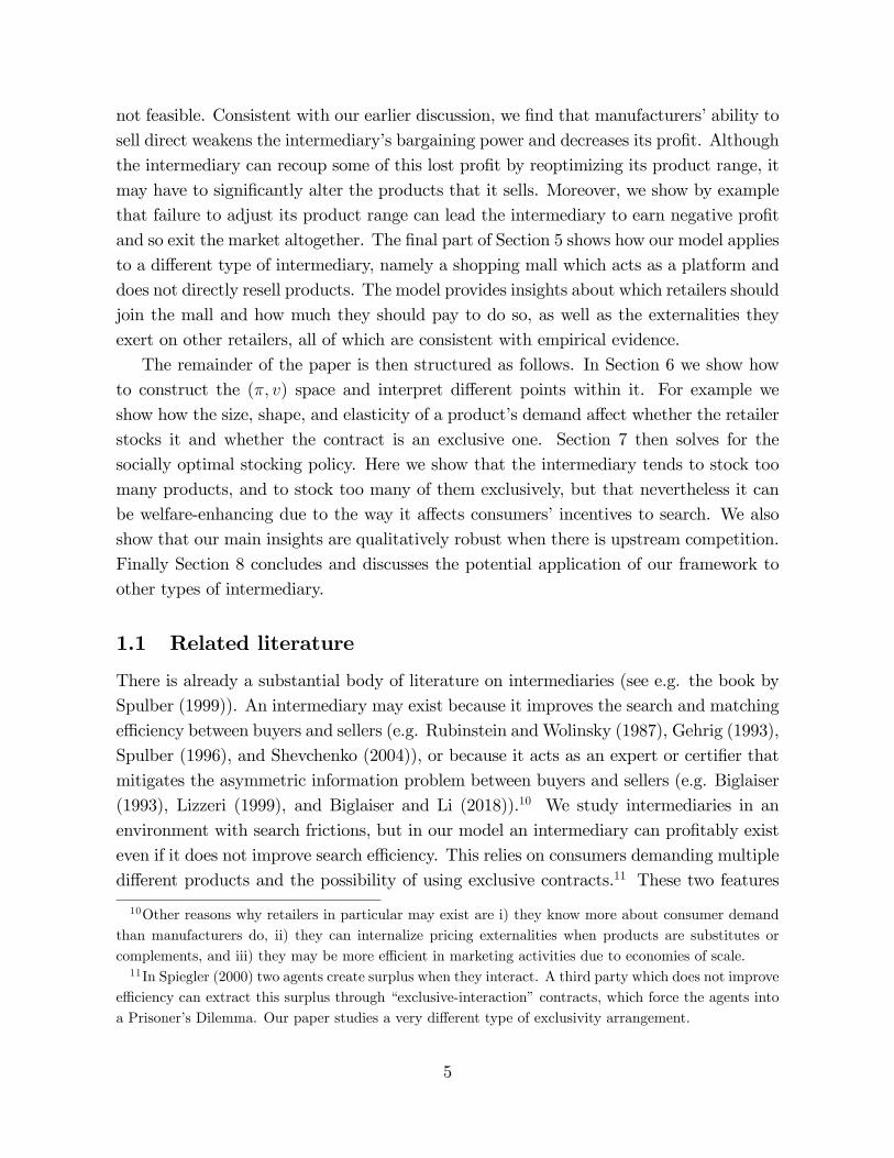
not feasible. Consistent with our earlier discussion, we �nd that manufacturers�ability tosell direct weakens the intermediary�s bargaining power and decreases its pro�t. Althoughthe intermediary can recoup some of this lost pro�t by reoptimizing its product range, itmay have to signi�cantly alter the products that it sells. Moreover, we show by examplethat failure to adjust its product range can lead the intermediary to earn negative pro�tand so exit the market altogether. The �nal part of Section 5 shows how our model appliesto a di¤erent type of intermediary, namely a shopping mall which acts as a platform anddoes not directly resell products. The model provides insights about which retailers shouldjoin the mall and how much they should pay to do so, as well as the externalities theyexert on other retailers, all of which are consistent with empirical evidence.The remainder of the paper is then structured as follows. In Section 6 we show how

to construct the (�; v) space and interpret di¤erent points within it. For example weshow how the size, shape, and elasticity of a product�s demand a¤ect whether the retailerstocks it and whether the contract is an exclusive one. Section 7 then solves for thesocially optimal stocking policy. Here we show that the intermediary tends to stock toomany products, and to stock too many of them exclusively, but that nevertheless it canbe welfare-enhancing due to the way it a¤ects consumers�incentives to search. We alsoshow that our main insights are qualitatively robust when there is upstream competition.Finally Section 8 concludes and discusses the potential application of our framework toother types of intermediary.

1.1 Related literature

There is already a substantial body of literature on intermediaries (see e.g. the book bySpulber (1999)). An intermediary may exist because it improves the search and matchinge¢ ciency between buyers and sellers (e.g. Rubinstein andWolinsky (1987), Gehrig (1993),Spulber (1996), and Shevchenko (2004)), or because it acts as an expert or certi�er thatmitigates the asymmetric information problem between buyers and sellers (e.g. Biglaiser(1993), Lizzeri (1999), and Biglaiser and Li (2018)).10 We study intermediaries in anenvironment with search frictions, but in our model an intermediary can pro�tably existeven if it does not improve search e¢ ciency. This relies on consumers demanding multipledi¤erent products and the possibility of using exclusive contracts.11 These two features

10Other reasons why retailers in particular may exist are i) they know more about consumer demandthan manufacturers do, ii) they can internalize pricing externalities when products are substitutes orcomplements, and iii) they may be more e¢ cient in marketing activities due to economies of scale.11In Spiegler (2000) two agents create surplus when they interact. A third party which does not improve

e¢ ciency can extract this surplus through �exclusive-interaction�contracts, which force the agents intoa Prisoner�s Dilemma. Our paper studies a very di¤erent type of exclusivity arrangement.

5

distinguish our model from existing work on intermediaries. Since our main focus is theretail market, we also study optimal product range and the impact of DTC sales, neitherof which are typically addressed by the intermediary literature.The mechanism by which an intermediary makes pro�t from stocking multiple prod-

ucts is reminiscent of bundling (e.g. Stigler (1968), Adams and Yellen (1976), McAfee et al(1989), and Chen and Riordan (2013)). By stocking some products that consumers valuehighly but are not available elsewhere, the intermediary forces consumers to visit and buyother low-value (but fairly pro�table) products as well which consumers would otherwisenot buy. However since our paper focuses on product selection, it is more related to thequestion of which products a �rm should bundle, something which is rarely discussed inthe bundling literature. Rayo and Segal (2010) use the same bundling argument in adi¤erent setting with information design. They show that an information platform oftenprefers partial information disclosure, in the sense of pooling two negatively correlatedprospects into one signal. (For example a search engine may pool a high-relevance butlow-pro�t ad with a low-relevance but high-pro�t ad.) Unlike us, they consider a discreteframework and (more importantly) they allow the information platform to send an arbi-trary number of signals (which in our framework, would be like allowing the intermediaryto organize and sell non-overlapping products in multiple stores). Consequently their op-timization problem is very di¤erent from ours. Moreover many other important featuresof our model, such as the role of exclusivity and the importance of search economies, haveno counterpart in their paper (or in the wider bundling literature).Our paper is also related to the growing literature on multiproduct search (e.g. McAfee

(1995), Shelegia (2012), Zhou (2014), Rhodes (2015), and Kaplan et al (2016)). Existingpapers usually investigate how multiproduct consumer search a¤ects multiproduct retail-ers�pricing decisions when their product range is exogenously given. Our paper departsfrom this literature by focusing on product range choice, another important decision formultiproduct retailers.12 Moreover our paper introduces manufacturers and so explicitlymodels the vertical structure of the retail market. In this sense it is also related to recentresearch on consumer search in vertical markets such as Janssen and Shelegia (2015),and Asker and Bar-Isaac (2017), though those works consider single-product search andaddress very di¤erent economic questions.Finally, our paper is also related to research on product assortment in operations

research and marketing (see e.g. the survey by Kök et al (2015)). Typically this literaturefocuses on a situation where consumers demand a single product, and studies the optimalnumber of (symmetric) varieties of that product to stock. Our paper focuses instead on a

12Rhodes and Zhou (2017) also study retailers�endogenous product range, but they consider a stylizedmerger setup with only two products.

6

retailer�s optimal product range choice when consumers have multiproduct demand. Westudy this issue with explicit upstream manufacturers and consumer shopping frictions,neither of which is usually considered in the above mentioned literature.13

2 The Model

There is a continuum of manufacturers with measure one, and each produces a di¤erentproduct. Manufacturer i has constant marginal cost ci � 0. There is also a unit mass ofconsumers, who are interested in buying every product. The products are independent,and each consumer wishes to buy Qi(pi) units of product i when its price is pi. Whena consumer buys multiple products, her surplus is additive over these products. Weassume that Qi(pi) is downward-sloping and well-behaved such that (pi � ci)Qi(pi) issingle-peaked at the monopoly price pmi . Per-consumer monopoly pro�t and consumersurplus from product i are respectively denoted by

�i � (pmi � ci)Qi(pmi ) and vi �Z 1

pmi

Qi(p)dp . (1)

Manufacturers can sell their product direct to consumers, for example via their ownretail outlet.14 (We consider the case where DTC sales are infeasible in Section 5.1.) Inaddition there is a single intermediary, which can buy products from manufacturers andresell them to consumers. The intermediary has no resale cost, but can stock at most ameasure �m � 1 of the products. We assume that the intermediary has all the bargainingpower, and simultaneously makes take-it-or-leave-it o¤ers to each manufacturer whoseproduct it wishes to stock.15 These o¤ers can be either �exclusive�(meaning that only theintermediary can sell the product to consumers) or �non-exclusive�(meaning that both theintermediary and the relevant manufacturer can sell the product to consumers). In bothcases we suppose that the intermediary o¤ers two-part tari¤s, consisting of a wholesaleunit price � i and a lump-sum fee Ti. The intermediary also informs manufacturers aboutwhich products it intends to stock, and whether it intends to stock them exclusively or

13Bronnenberg (2017) considers a model where consumers like variety but dislike shopping, so retailersstock multiple varieties to reduce consumers�shopping costs. His model is otherwise very di¤erent fromours, as are the questions it studies. For example in his model varieties are symmetric, and so he doesnot look at the optimal composition of a retailer�s product line.14Alternatively, we can interpret direct sales as a manufacturer selling through an independent single-

product retailer. If the manufacturer can make a take-it-or-leave-it o¤er to the independent retailer, allour analysis and results remain unchanged.15Our results do not change qualitatively if instead the intermediary and manufacturer share any pro�ts

that are earned from sales of the latter�s product.

7

non-exclusively.16 Manufacturers who received an o¤er then simultaneously accept orreject.Consumers know where each product is available, but do not observe the terms of

any upstream contracts. Moreover consumers cannot observe a �rm�s price(s) or buy itsproduct(s) without incurring a search cost.17 Consumers di¤er in terms of their �unit�search cost s, which is distributed in the population according to a cumulative distri-bution function F (s) with support (0; s]. The corresponding density function f(s) iseverywhere di¤erentiable, strictly positive, and uniformly bounded with maxs f(s) <1.If a consumer searches a measure n of manufacturers, she incurs a total search cost n� s.If a consumer also searches the intermediary, and the intermediary stocks a measure m ofproducts, she incurs an additional search cost h(m) � s. We can thus interpret s as theopportunity cost of time, with the time needed to buy from a manufacturer normalizedto 1, and the time needed to visit the intermediary equal to h (m).18 We assume thatthe function h (m) is positive and weakly increasing, re�ecting the idea that larger storesmay take longer to navigate, and may also be located further out of town. (Notice thatwe allow for the case where h (m) is constant and so independent of the intermediary�ssize. Below we provide a microfoundation for why h (m) might be strictly increasing.)We also introduce the following notation: when h (m) =m < 1 the intermediary generateseconomies of search, and when h (m) =m > 1 it generates diseconomies of search. Finallyas is standard, we assume that after searching consumers may costlessly recall past o¤ers.The timing of the game is as follows. At the �rst stage, the intermediary simulta-

neously makes o¤ers to manufacturers whose product it would like to stock. An o¤erspeci�es (� i; Ti) and whether the intermediary will sell the product exclusively or not.Manufacturers then simultaneously accept or reject. At the second stage, all �rms thatsell to consumers choose a retail price for each of their products. The intermediary useslinear pricing. At the third stage, consumers observe who sells what and form (rational)expectations about all retail prices. They then search sequentially among �rms and maketheir purchases. We assume that if consumers observe an unexpected price at some �rm,they hold passive beliefs about the retail prices they have not yet discovered.

16This assumption aims to capture the idea that in practice negotiations evolve over time, such thatmanufacturers can (roughly) observe what other products the intermediary stocks.17Our assumptions here try to capture the idea that a retailer�s product range is usually reasonably

steady over time, whilst its prices �uctuate more frequently for example due to cost or demand shocks.18More generally, the time needed to buy from a manufacturer can vary across products. One possible

way to deal with that case is to use a triplet (�; v; �) to characterize a product where � is the amountof time needed for a consumer to buy from its manufacturer. Intuitively, all else equal a product withhigher � is more likely to be carried by the intermediary.

8

2.1 Preliminary analysis

We start with the following useful result. (All omitted proofs are in the appendix.)

Lemma 1 (i) In any equilibrium where each product market is active, each seller of aproduct charges consumers the relevant monopoly price.(ii) If product i is stocked exclusively by the intermediary, the intermediary o¤ers themanufacturer (� i = ci; Ti = �iF (vi)). If product i is stocked non-exclusively by the inter-mediary, in terms of studying the optimal product range, it is without loss of generalityto focus on the contracting outcome where the intermediary o¤ers (� i = ci; Ti) to manu-facturer i, such that the manufacturer�s total payo¤ is �iF (vi).

To understand the intuition behind Lemma 1, recall that a product can be sold in threedi¤erent ways. Firstly product i may be sold only by its manufacturer. Since consumersonly learn the manufacturer�s price after they have sunk their search cost, it is optimal forthe manufacturer to charge the monopoly price pmi .

19 This is just the standard hold-upproblem which arises in search models (see e.g. Stiglitz (1979) and Anderson and Renault(2006)). Consumers therefore rationally anticipate monopoly pricing and so, using thenotation introduced in (1), search if and only if s � vi. Consequently the manufacturer�sequilibrium pro�t is �iF (vi). Notice that this is also the manufacturer�s outside optionif the intermediary makes it an o¤er.Continuing with the intuition for Lemma 1, secondly product i may be sold exclusively

by the intermediary. Since consumers do not observe the price before searching, the samehold-up argument implies that if the intermediary faces a wholesale price � i, it will chargethe corresponding monopoly price argmax (p� � i)Qi (p). Notice that joint pro�t earnedon product i is maximized when the intermediary charges the monopoly price pmi , thereforein order to induce this outcome the intermediary proposes � i = ci i.e. a bilaterally e¢ cienttwo-part tari¤. The intermediary then drives the manufacturer down to its outside optionby o¤ering it a lump-sum payment Ti = �iF (vi). Thirdly product i may be sold by bothits manufacturer and the intermediary. The analysis here is more complex. However themain idea is that the intermediary again avoids double-marginalization by proposing acontract with � i = ci, whilst search frictions eliminate price competition between themanufacturer and intermediary. In particular, following Diamond�s (1971) paradox ifconsumers expect both sellers to charge the same price for product i, they will search atmost one of them and hence each �nds it optimal to charge the monopoly price. The

19As is usual in search models, there also exist other equilibria in which consumers do not search (some)sellers because they are expected to charge very high prices, and given no consumers search these highprices can be trivially sustained. We do not consider these uninteresting equilibria in this paper.

9

manufacturer is compensated for any sales that it loses in signing the contract by way ofa lump-sum transfer.Given Lemma 1, it is convenient to index products by their per-consumer monopoly

pro�t and consumer surplus as de�ned in (1) (rather than by their demand curve Qi (pi)and cost ci). This helps convert the potentially complicated product space into a two-dimensional one. Henceforth let � R2+ be a two-dimensional product space (�; v), andsuppose it is compact and convex. Let v � 0 and v <1 be the lower and the upper boundof v. For each v 2 [v; v], there exist 0 � �(v) � �(v) < 1 such that � 2 [�(v); �(v)].(In section 6 we provide examples of demand functions which can generate this type ofproduct space.) Let (;F ; G) be a probability measure space where F is a �-�eld which isthe set of all measurable subsets of according to measure G. (In particular, G() = 1.)When there is no confusion, we also use G to denote the joint distribution function of(�; v), and let g be the corresponding joint density function. We assume that g is di¤er-entiable and strictly positive everywhere. If a consumer buys a set A 2 F of products attheir monopoly prices, she obtains surplus

RAvdG before taking into account the search

cost. To avoid trivial corner solutions, we also assume that v � s.

Discussion. Before solving for the intermediary�s optimal product range, we �rstdiscuss some of our modeling assumptions and their implications.(i) A continuum of products. Considering a continuum of products is mainly for

analytical convenience. A model with a discrete number of products f(�i; vi)gi=1;:::;nwould yield qualitatively similar insights but be messier to solve because the optimizationproblem would become a combinatorial one.20

(ii) Homogeneous consumer demand. Consumers are assumed to demand all products.However in reality some consumers want to buy more products than others (and similarlysome products are needed more often than others). We could explicitly add this hetero-geneity into the model, but the analysis would be less tractable. Moreover our modelalready generates demand heterogeneity in the sense that consumers with a lower searchcost will end up buying more products.(iii) An instore-search microfoundation for h(m). Suppose there is a �xed cost �0s

of traveling to the intermediary, and also a cost �1s to search each product in the store.Also suppose the intermediary can in�uence the consumer search order e.g. via whereit places di¤erent products within the store. We can show that by forcing consumers tosearch exclusive products with high v last, the intermediary can induce every consumer

20See footnote 27 later for the details. The case with only two products is easy to deal with, but is notrich enough to study the optimal product range choice in a meaningful way.

10

who visits to search all its products.21 Consumers anticipate this, and so the total cost ofsearching the intermediary is h(m)s with h(m) = �0 + �1m, which is strictly increasingprovided �1 > 0.(iv) Lemma 1 and monopoly pricing. The monopoly pricing outcome described in

Lemma 1 enables us to represent products using the (�; v) space, and hence study productrange choice in a tractable way. However notice that monopoly pricing is not importantper se - what really matters for our analysis is that the retail price of each productremains the same irrespective of where it is sold. (For instance this could be the casewhen there is a resale price agreement between the manufacturer and the retailer.) Ofcourse in practice prices can di¤er across retail outlets, and a large literature alreadyexplores this. Our model abstracts from such price dispersion in order to make progressin understanding optimal product choice.

3 A Simple Case

We now study the intermediary�s optimal product range choice. We start with a specialcase where i) the intermediary can only o¤er exclusive contracts, ii) h (m) = m such thatthe intermediary generates no economies of search, and iii) �m = 1 such that there is nostocking space limit. This relatively simple case helps to illustrate some of the economicforces in�uencing optimal product selection.We �rst solve for a consumer�s decision of whether or not to search the intermediary.

Suppose the intermediary sells a positive measure of products A 2 F . If a consumer visitsthe intermediary, she will buy all products available there and so obtain an additionalutility

RAvdG, but at the same time she also incurs an additional search cost s

RAdG.

Consequently a consumer visits the intermediary if and only if s � k, where

k =

RAvdGRAdG

(2)

is the average consumer surplus amongst the products sold at the intermediary. (Notethat the consumer will search any product i 62 A if and only if s � vi, and that the orderin which she searches through the intermediary and manufacturers does not matter.)The intermediary�s problem is then to

maxA2F

ZA

� [F (k)� F (v)] dG ; (3)

21Further details are available on request. This is similar to the idea of search diversion in Hagiu andJullien (2011).

11

with k de�ned in (2).22 In particular the intermediary earns a net pro�t � [F (k)� F (v)]from product (�; v) if it stocks it. This is explained as follows. The intermediary attractsa mass of consumers F (k), and so earns variable pro�t �F (k). However from Lemma 1the intermediary must also compensate the relevant manufacturer with a lump-sum trans-fer �F (v). The following simple observation will play an important role in subsequentanalysis: among the products stocked by the intermediary, those with v < k generate apro�t while those with v > k generate a loss. Intuitively a product with v < k generatesrelatively few sales when sold by its manufacturer, since consumers anticipate receivingonly a low surplus. When the same product is sold by the intermediary its sales increase,because more consumers search the intermediary (given its higher expected surplus k).The opposite is true for a product with v > k, i.e. its demand is shrunk when sold throughthe intermediary.23

The following lemma is a useful �rst step in characterizing the intermediary�s optimalproduct range.

Lemma 2 The intermediary makes a strictly positive pro�t. It sells a strictly positivemeasure of products but not all products (i.e.

RAdG 2 (0; 1)).

The intermediary earns strictly positive pro�t even though its search technology is nomore e¢ cient than that of the manufacturers whose products it resells.24 To understandwhy, recall that the intermediary always makes a gain on the low-v products and a losson the high-v products, and that these gains and losses are proportional to a product�sper-customer pro�tability �. Now imagine that the intermediary selects its pro�t-makingproducts amongst those with high �, and selects its loss-making products amongst thosewith low �. This strategy seeks to maximize gains on the former, and minimize losseson the latter, and so might be expected to generate a net positive pro�t. In the proofwe show by construction that there is always some set A where this logic is correct. Onthe other hand, even with no stocking space constraint, the intermediary never stocks allproducts.We now solve explicitly for the optimal set of products stocked by the intermediary.

Instead of working directly with areas in , it is more convenient to introduce a stockingpolicy function q (�; v) 2 f0; 1g. Then stocking products in a set A 2 F is equivalent toadopting a measurable stocking policy function where q(�; v) = 1 if and only if (�; v) 2 A.22When

RAdG = 0 intermediary pro�t is zero regardless of how we specify k. In some later analysis we

consider limit cases where the measure of A goes to zero, and k will be well-de�ned via L�hopital�s rule.23The same is true for a general h(m) if it increases fast enough in m. However if h(m) is (close to)

constant and su¢ ciently small, k can be greater than any v in A. We consider this case in Section 4.24By continuity the same is true even when the intermediary�s search technology is slightly less e¢ cient.

12

The intermediary�s problem then becomes

maxq(�;v)2f0;1g

Z

q(�; v)�[F (k)� F (v)]dG ;

where the average consumer surplus k o¤ered by the intermediary solvesZ

q(�; v) (v � k) dG = 0 : (4)

This is an optimization of functionals. It can be shown that this optimization problemhas a solution, and the optimal solution can be derived by treating (4) as a constraintand using the following Lagrange method.The Lagrangian function is

L =Z

q(�; v) [� [F (k)� F (v)] + �(v � k)] dG ; (5)

where � is the Lagrange multiplier associated with the constraint (4). The �rst term� [F (k)� F (v)] is the direct e¤ect on pro�t of stocking product (�; v). The second term�(v�k) re�ects the indirect e¤ect from the in�uence on consumer search behavior (where� > 0 as we will see below), and it captures the cross-product externalities in our model.For products with v < k their direct e¤ect is positive as we explained before, while theirindirect e¤ect is negative because stocking them reduces the average surplus o¤ered bythe intermediary and so causes less consumers to search it. The opposite is true for theproducts with v > k. Since the integrand in (5) is linear in q, the optimal stocking policyis as follows:

q(�; v) =

(1 if � [F (k)� F (v)] + �(v � k) � 00 otherwise

:

For given k and �, let I(k; �) denote the set of (�; v) for which q(�; v) = 1. It consistsof the following two regions:

v < k and � � � k � vF (k)� F (v) ; (6)

andv > k and � � � k � v

F (k)� F (v) : (7)

(Notice that the intermediary is indi¤erent about whether or not to stock products withv = k.) Therefore the intermediary�s optimal product selection consists of two �negativelycorrelated� regions in the product space.25 First, the intermediary stocks products in

25The horizontal line � (k � v) = [F (k)� F (v)] which divides up the product space is continuous in v,and upward (downward) sloping when F (s) is concave (convex).

13

the bottom-right corner with high v and low �. These products are used to induceconsumers to search, but since they have v > k they make a loss and so the intermediaryminimizes this by choosing those with the lowest possible �. Second, the intermediarystocks products in the top-left corner with low v and high �. Since these products havev < k they make a pro�t, and so the intermediary maximizes this by choosing those withthe highest possible �. Products in other parts of the product space are not stocked:those with low v and low � would generate little direct pro�t yet dissuade consumersfrom searching, and those with high v and high � are too expensive to buy from theirmanufacturers.It then remains to determine k and �. Firstly, at the optimum we must have F (k) 2

(0; 1). This is because Lemma 2 shows that I(k; �) has strictly positive measure, whichfrom the de�nition of k implies k 2 (v; v), and moreover by assumption s 2 (0; �s] where�s � �v. Since k is interior, we can take the �rst-order condition of (5) with respect to k,and obtain Z

I(k;�)

(f(k)� � �)dG = 0 ; (8)

whereupon we observe that � > 0.26 Secondly, we have the original constraint (4), whichwe can rewrite as Z

I(k;�)

(v � k)dG = 0 : (9)

We therefore have a system of two equations (8) and (9) in two unknowns. If the systemhas multiple solutions, the solution that generates the highest pro�t is the optimal one.The following result summarizes the above analysis:27

Proposition 1 The intermediary optimally stocks products in the regions of (6) and (7),where k 2 (v; v) and � > 0 jointly solve equations (8) and (9).

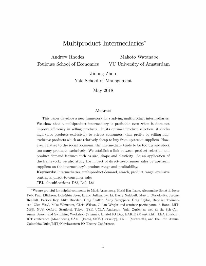
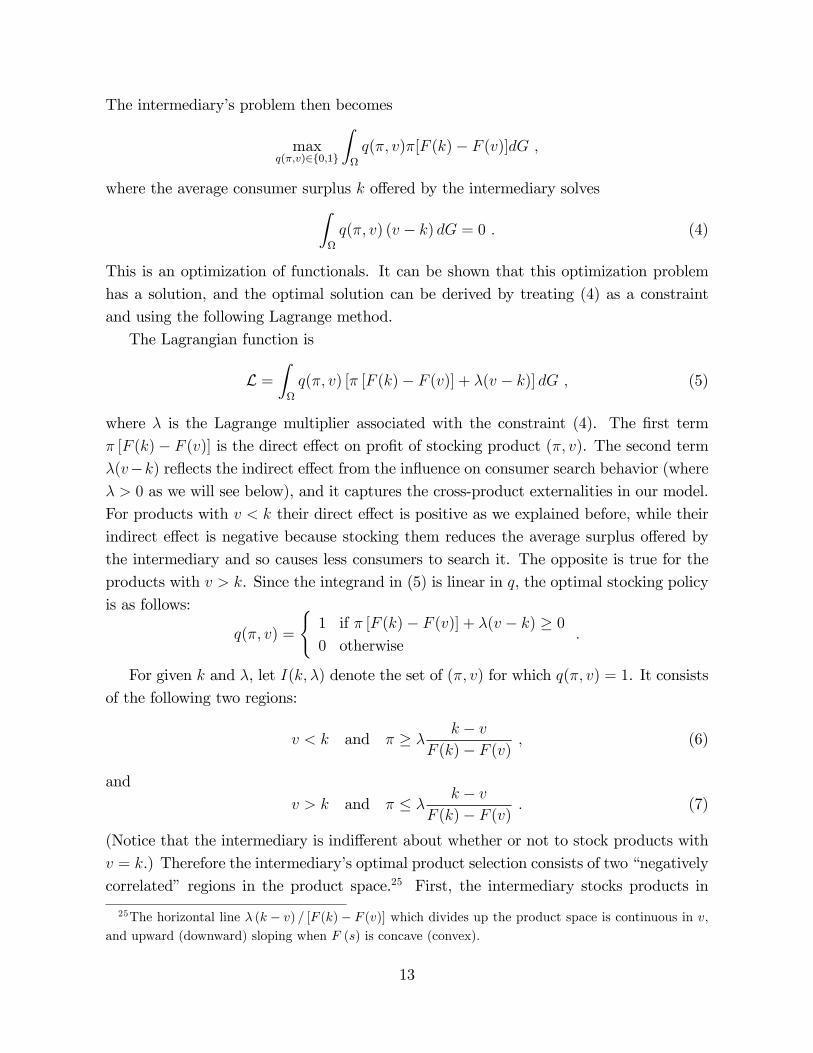
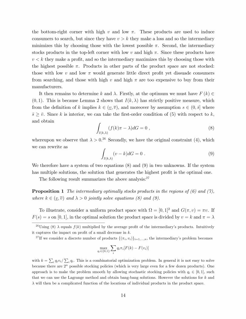
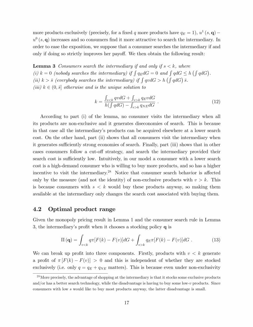
To illustrate, consider a uniform product space with = [0; 1]2 and G(�; v) = �v. IfF (s) = s on [0; 1], in the optimal solution the product space is divided by v = k and � = �

26Using (8) � equals f(k) multiplied by the average pro�t of the intermediary�s products. Intuitivelyit captures the impact on pro�t of a small decrease in k.27If we consider a discrete number of products f(�i; vi)gi=1;:::;n, the intermediary�s problem becomes

maxqi2f0;1g

Xi

qi�i[F (k)� F (vi)]

with k =P

i qivi=P

i qi. This is a combinatorial optimization problem. In general it is not easy to solvebecause there are 2n possible stocking policies (which is very large even for a few dozen products). Oneapproach is to make the problem smooth by allowing stochastic stocking policies with qi 2 [0; 1], suchthat we can use the Lagrange method and obtain bang-bang solutions. However the solutions for k and� will then be a complicated function of the locations of individual products in the product space.

14

with k = � = 12. If F (s) =

ps on [0; 1], in the optimal solution the product space is

divided by v = k and � = �(pk+

pv) with k � 0:4876 and � � 0:3515. The shaded areas

in Figure 1 below depict the optimal product range in these two examples. In the �rstexample the intermediary makes pro�t 0:03125 and improves industry pro�t by 12:5%relative to the case of no intermediary, and in the second example the intermediary makespro�t of about 0:036 and improves industry pro�t by about 10:8%.In this simple case the intermediary harms consumers, because it does not generate any

search e¢ ciencies and at the same time restricts consumer choice. Speci�cally, consumerswith s < k who search the intermediary are forced to buy some low-v products whichthey otherwise would not buy. Similarly consumers with s > k who do not search theintermediary are unable to buy some attractive high-v products which are now onlyavailable at the intermediary. Nevertheless the intermediary may improve total welfare,de�ned as the sum of industry pro�t and consumer surplus. Indeed this is the case in bothof the above numerical examples, where total welfare increases by about 2:5% and 2:8%respectively. Intuitively, in the absence of an intermediary consumers search too little:they search and buy a product (�; v) only if s < v, but from a total welfare perspectivethey should do so whenever s < � + v. Moreover amongst products with the same � + v,this problem of �under search� is more severe for those with low-v and high-�. Sincethe intermediary�s optimal product selection leads to an expansion in demand for theseproducts, its presence can increase total welfare. Nevertheless the intermediary does notaccount for the harm it imposes on consumers with s > k and so its product selectionis not socially optimal. We will discuss the socially optimal product selection in Section7.1.

0.0 0.2 0.4 0.6 0.8 1.00.0

0.2

0.4

0.6

0.8

1.0

v

pi

(a) F (s) = s

0.0 0.2 0.4 0.6 0.8 1.00.0

0.2

0.4

0.6

0.8

1.0

v

pi

(b) F (s) =ps

Figure 1: Optimal product range: the simple case

15

4 The General Case

We now characterize the optimal product selection in the general case in which i) theintermediary can o¤er both exclusive and non-exclusive contracts, ii) the cost of searchingthe intermediary is h (m)� s with h(m) weakly increasing, and iii) there is a limit �m onthe measure of products the intermediary can stock. Let q(�; v) = (qE (�; v) ; qNE (�; v))denote the stocking policy function, where qE (�; v) 2 f0; 1g and qNE (�; v) 2 f0; 1g. Inparticular qE (�; v) = 1 if and only if product (�; v) is stocked exclusively, and similarlyqNE (�; v) = 1 if and only if product (�; v) is stocked non-exclusively. (Note that for eachproduct (�; v) at most one of qE (�; v) and qNE (�; v) can be 1, but both can be 0 in whichcase the product is not stocked at all.) It is again convenient to let

q(�; v) � qE(�; v) + qNE(�; v) 2 f0; 1g

denote whether or not product (�; v) is stocked. Henceforth whenever there is no confusionwe will suppress the arguments (�; v) in the stocking policy function.

4.1 Consumer search behavior

We �rst solve for consumers�optimal search rule given a stocking policy q. Recall fromLemma 1 that all sellers of a product charge the same price. Hence a consumer willnever search both the intermediary and a manufacturer whose product is stocked there.Moreover if a consumer does consider searching a manufacturer, she will do so only ifv > s. It is also straightforward to see that the order in which a consumer visits thevarious manufacturers and the intermediary does not matter. Therefore a consumer whosearches the intermediary gets an expected surplus

u1 (s;q) =

ZqvdG� h

�ZqdG

�s+

Zv>s

(1� q) (v � s) dG ; (10)

where the �rst two terms are surplus obtained directly from the intermediary, and the�nal term is surplus obtained by searching products not available at the intermediary.Notice that only q = qE + qNE matters, and not whether products are stocked exclusivelyor non-exclusively.At the same, a consumer who does not search the intermediary gets expected surplus

u0 (s;q) =

Zv>s

(1� qE) (v � s) dG ; (11)

because she can only buy products which are available from their manufacturers (and soare not stocked exclusively by the intermediary). Notice that when the intermediary stocks

16

more products exclusively (precisely, for a �xed q more products have qE = 1), u1 (s;q)�u0 (s;q) increases and so consumers �nd it more attractive to search the intermediary. Inorder to ease the exposition, we suppose that a consumer searches the intermediary if andonly if doing so strictly improves her payo¤. We then obtain the following result:

Lemma 3 Consumers search the intermediary if and only if s < k, where(i) k = 0 (nobody searches the intermediary) if

RqEdG = 0 and

RqdG � h

�RqdG

�.

(ii) k > �s (everybody searches the intermediary) ifRqvdG > h

�RqdG

��s.

(iii) k 2 (0; �s] otherwise and is the unique solution to

k =

Rv<k

qvdG+Rv>k

qEvdG

h(RqdG)�

Rv>k

qNEdG: (12)

According to part (i) of the lemma, no consumer visits the intermediary when allits products are non-exclusive and it generates diseconomies of search. This is becausein that case all the intermediary�s products can be acquired elsewhere at a lower searchcost. On the other hand, part (ii) shows that all consumers visit the intermediary whenit generates su¢ ciently strong economies of search. Finally, part (iii) shows that in othercases consumers follow a cut-o¤ strategy, and search the intermediary provided theirsearch cost is su¢ ciently low. Intuitively, in our model a consumer with a lower searchcost is a high-demand consumer who is willing to buy more products, and so has a higherincentive to visit the intermediary.28 Notice that consumer search behavior is a¤ectedonly by the measure (and not the identity) of non-exclusive products with v > k. Thisis because consumers with s < k would buy these products anyway, so making themavailable at the intermediary only changes the search cost associated with buying them.

4.2 Optimal product range

Given the monopoly pricing result in Lemma 1 and the consumer search rule in Lemma3, the intermediary�s pro�t when it chooses a stocking policy q is

�(q) =

Zv<k

q�[F (k)� F (v)]dG+Zv>k

qE�[F (k)� F (v)]dG : (13)

We can break up pro�t into three components. Firstly, products with v < k generatea pro�t of � [F (k)� F (v)] > 0 and this is independent of whether they are stockedexclusively (i.e. only q = qE + qNE matters). This is because even under non-exclusivity

28More precisely, the advantage of shopping at the intermediary is that it stocks some exclusive productsand/or has a better search technology, while the disadvantage is having to buy some low-v products. Sinceconsumers with low s would like to buy most products anyway, the latter disadvantage is small.

17

the manufacturer makes zero direct sales, since consumers with s < k buy its productfrom the intermediary and consumers with s � k are not willing to search it. Hence theintermediary earns revenue �F (k), and must pay the manufacturer the full pro�t �F (v)that it would earn by rejecting the o¤er. Secondly, products with v > k that are stockedexclusively generate a negative pro�t of � [F (k)� F (v)] < 0, and the explanation is thesame as in the simple case. Lastly, products with v > k that are stocked non-exclusivelygenerate zero pro�t and so do not appear in equation (13). The reason is that when amanufacturer signs a non-exclusive contract, consumers with s < k switch and buy itsproduct from the intermediary, but consumers with s 2 (k; v) continue to buy direct fromit. Hence the intermediary only needs to compensate the manufacturer by �F (k), whichis exactly its own revenue from selling that product. Note that although the intermediarybreaks even on these products, it may have an incentive to stock them in order to in�uenceconsumer search behavior. (We show later in Section 7.2 that with upstream competitioneven these non-exclusive products can generate a pro�t.)The following lemma shows that the intermediary is guaranteed to earn strictly pos-

itive pro�t provided there is some feasible store size ~m where it does not generate strictdiseconomies of search.29

Lemma 4 The intermediary stocks a strictly positive measure of products and earns astrictly positive pro�t if there exists an ~m 2 (0; �m) such that h ( ~m) � ~m.

We now proceed to characterize the optimal product selection when the intermediarycan pro�tably exist with k > 0 (e.g. when the condition in Lemma 4 is satis�ed). Theintermediary wishes to maximize its pro�t from equation (13) given the space limit �m � 1,where k was de�ned earlier in Lemma 3. When k 2 (0; �s] we know that k satis�es equation(12), which we can rewrite asZ

v<k

qvdG+

Zv>k

(qEv + qNEk)dG� h(m)k = 0 ; (14)

where m denotes the measure of products stocked by the intermediary and satis�es

m =

ZqdG : (15)

The stocking space constraint can be written as

m � �m : (16)

29Note that this is only a simple su¢ cient condition for the existence of the intermediary. In thenumerical examples below we provide weaker su¢ cient conditions.

18

It is again convenient to solve the intermediary�s problem using the Lagrangian method,where we treat (14)-(16) as constraints. Let �, � and � be their respective Lagrange mul-tipliers. After some simple manipulations we can write the (Kuhn-Tucker) Lagrangefunction as

L =

Zv<k

q f� [F (k)� F (v)] + �v � �g dG

+

Zv>k

fqE [� [F (k)� F (v)] + �v � �] + qNE (�k � �)g dG

��kh(m) + �m+ �( �m�m) : (17)

(Note that if k > �s, the constraint (14) does not apply and so we set � = 0.) It is againuseful to understand this Lagrange function in terms of the direct and indirect e¤ects ofstocking a product. The direct e¤ect is the pro�t generated by this product: recall fromearlier that it is zero if the product is non-exclusive and v > k, and otherwise equals� [F (k)� F (v)]. The indirect e¤ect captures the e¤ect on consumer search behavior: itequals �k � � if the product is non-exclusive and v > k, and otherwise is �v � �. Sincethe integrands are again linear in q, or (qE; qNE), we have the following characterizationof the optimal product selection:

Proposition 2 Suppose the intermediary earns a strictly positive pro�t (e.g. the condi-tion in Lemma 4 is satis�ed). The optimal product selection is as follows (with k > 0,� � 0 and � � 0 de�ned in the appendix):(i) Products with v < k are stocked if and only if

� � �� �vF (k)� F (v) ; (18)

and it does not matter whether these products are exclusive or not.(ii) Products with v > k are stocked exclusively if and only if

� � maxf�k; �g � �vF (k)� F (v) : (19)

At the same time, if �k > � then all other products with v > k are stocked non-exclusively,if �k = � some of the other products with v > k are stocked non-exclusively, and if �k < �none of the other products with v > k are stocked.

As in the previous simple case, the intermediary stocks some high-v and low-� productsexclusively to attract consumers, and some low-v and high-� products to generate pro�ts.A major di¤erence is that now the intermediary may also stock high-v and high-� products

19

non-exclusively. Whether or not that happens depends on the sign of �k��, the indirecte¤ect of stocking products with v > k non-exclusively.30 ;31

In general it appears hard to �nd primitive conditions for the sign of �k � �, but wehave the following useful observation:

Corollary 1 If the space constraint is not binding (m < �m) in the optimal product se-lection, then � = �kh0 (m). In the region of v > k, all products are stocked (i.e. �k > �)if h0 (m) < 1, but only low-� products are stocked exclusively (i.e. �k < �) if h0 (m) > 1.

This result implies that with (marginal) diseconomies of search in visiting the inter-mediary the optimal product selection features two negatively correlated regions as in theprevious simple case: one with low-v and high-� products in the top-right corner and theother with high-v and low-� products in the bottom-right corner.32

Notice that in the region of v < k the intermediary is indi¤erent about whether to stocka product exclusively or non-exclusively, since exclusivity has no e¤ect on either the directpro�t generated (c.f. equation (13)) nor on consumer search behavior (c.f. Lemma 3). Oneway to break this indi¤erence is to introduce some small-demand consumers who nevervisit the intermediary. In that case the intermediary strictly prefers to stock productswith v < k non-exclusively, because it reduces the compensation paid to manufacturers.(A formal proof is available upon request.) Hence in the following we say that productswith v < k are stocked non-exclusively.We now illustrate the optimal product selection using some examples. First, we illus-

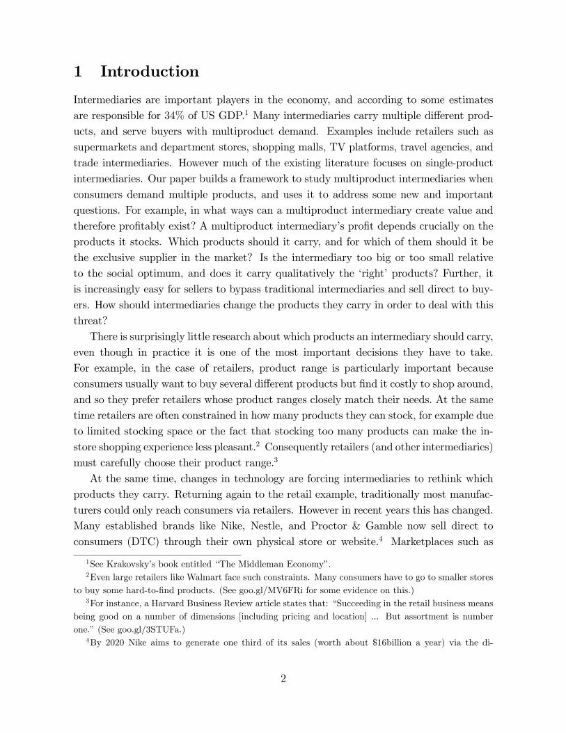
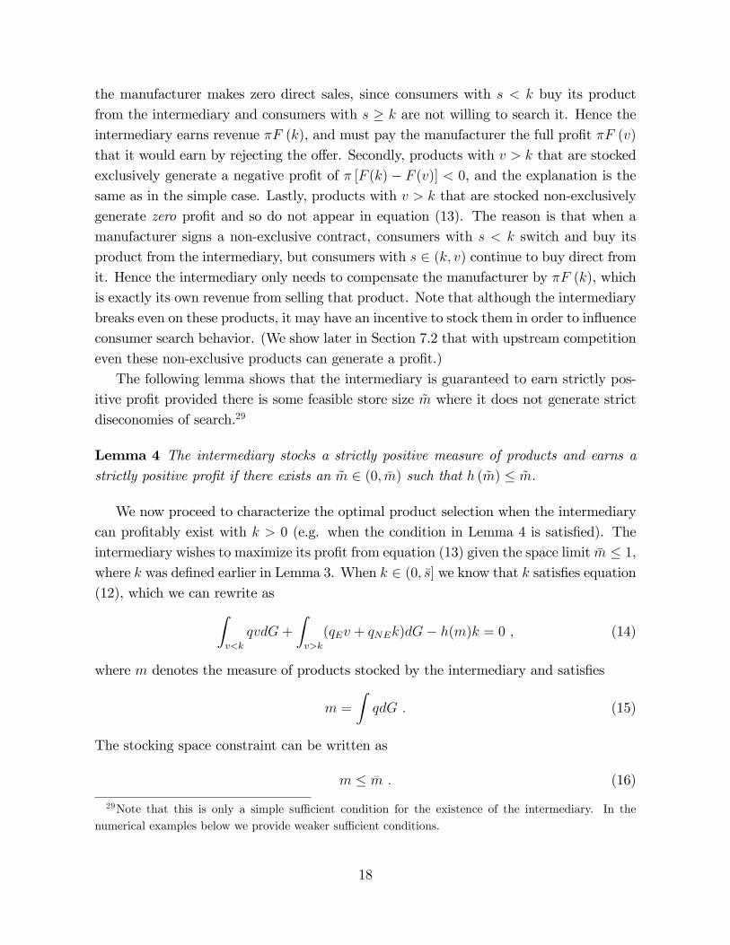
trate the result in Corollary 1 about how h0 (m) a¤ects the optimal stocking policy. Con-sider the case with F (s) = s and G(�; v) = �v, and suppose there is no space constraint(i.e. �m = 1) and h(m) = a+ bm with a; b � 0.33 In Figure 2(a) h(m) = 0:8m and so theintermediary generates economies of search. As shown in Corollary 1 we have �k > � andso all products with v > k are stocked. In Figure 2(b) h(m) = m as in the simple case we

30If �k � � = 0, the intermediary is indi¤erent about which of these non-exclusive products to select,and the equation �k � � = 0 is used to determine their measure. (Notice that in that case only themeasure of non-exclusively stocked products, instead of the exact composition, matters for both (12) and(17). Consequently the optimal selection is not unique.)31Another subtle di¤erence is that in this general case it is possible that k < v when v > 0 and

diseconomies of search are su¢ ciently strong, or k > v when economies of search are su¢ ciently strong.When this happens, only one part of the characterization in Proposition 2 is relevant.32When �k < � these two regions are also disconnected, because as v ! k the two thresholds in (18)

and (19) tend respectively to 1 and �1. Intuitively products with v close to k generate only a smalldirect pro�t or loss, but when for example h0 (m) > 1 their negative e¤ect on consumers�incentives tosearch the intermediary dominates.33This example can be fully solved. (Details are available upon request.) A su¢ cient condition for the

intermediary to exist in this example is a+ b � 32 , which is weaker than Lemma 4.

20

studied earlier. Here we have �k = � and so the intermediary is indi¤erent about whetherto stock each of the products in the top-right corner [0:5; 1]2 non-exclusively. We havedrawn the �gure for the case where all those products are stocked. Finally in Figure 2(c)h(m) = 1:2m and so the intermediary generates diseconomies of search. We now have�k < � and so there are only exclusive products in the region of v > k. Comparing acrossthese three cases, as the intermediary�s search technology becomes less e¢ cient it stocksfewer products (m decreases from 0:76 to 0:75 and then to 0:29) but a larger proportionof them are exclusive (the percentage increases from 27% to 33% and then to 50%).

E

NE

0.0 0.2 0.4 0.6 0.8 1.00.0

0.2

0.4

0.6

0.8

1.0

v

pi

(a) h(m) = 0:8m

E

NE

0.0 0.2 0.4 0.6 0.8 1.00.0

0.2

0.4

0.6

0.8

1.0

v

pi

(b) h(m) = m

NE

E

0.0 0.2 0.4 0.6 0.8 1.00.0

0.2

0.4

0.6

0.8

1.0

v

pi

(c) h(m) = 1:2m

Figure 2: Optimal product range with no space constraint

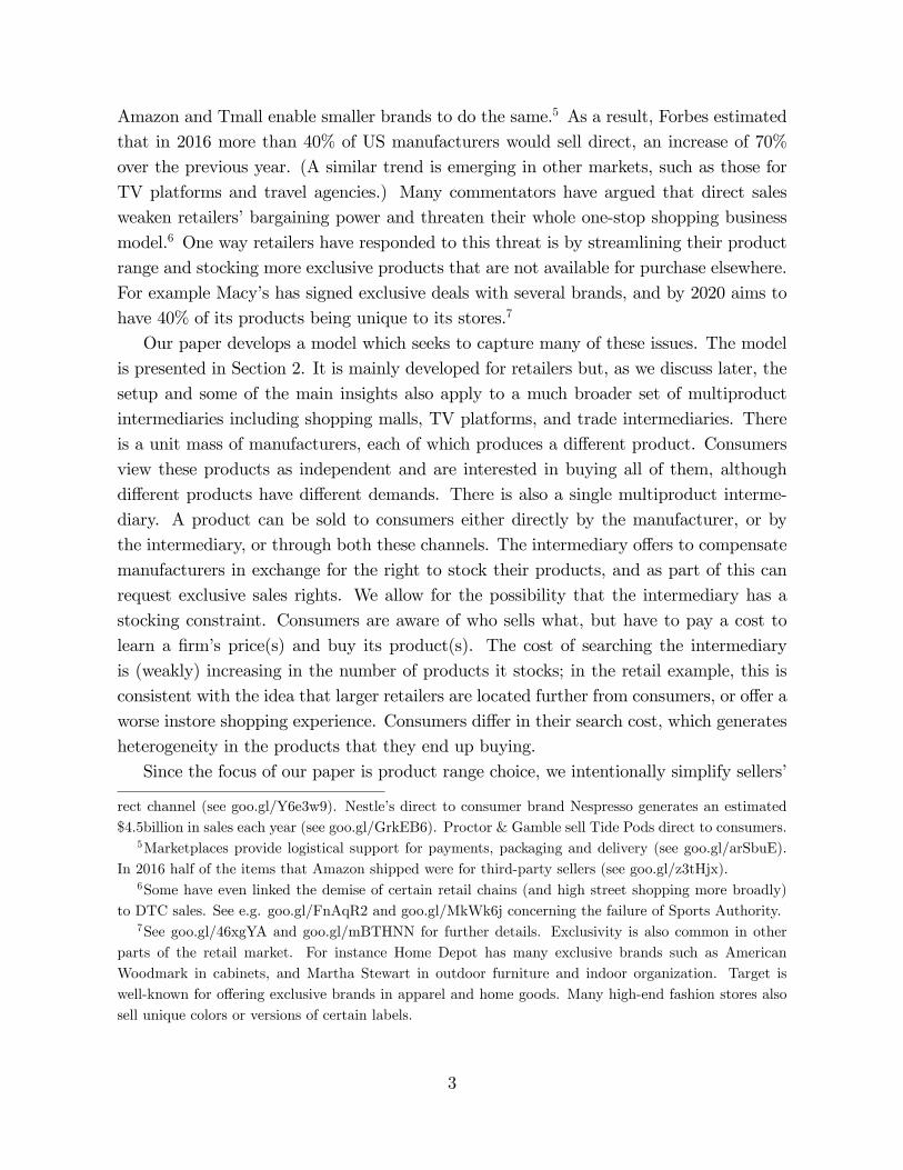
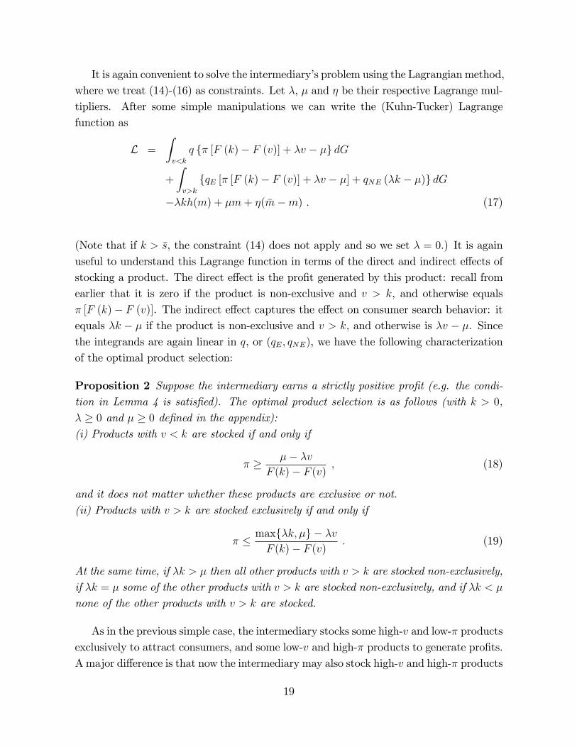
Second, we illustrate how the space limit �m a¤ects product selection. Consider againthe case with G(�; v) = �v and F (s) = s, but now suppose h (m) = 0:4. The marginaleconomies of search are so strong in this case that the intermediary will stock all products if�m = 1, and so the space constraint is always binding. Starting from �m = 1, as we reduce�m the intermediary �rst drops the products with low-v and low-�. When �m is aboveapproximately 0:65 we have that k > 1 and so all products are stocked non-exclusively.When �m is between around 0:65 and 0:463 we �nd that k < 1, and so as depicted inFigure 3(a) the intermediary starts to stock some products exclusively. At the same time�k � � > 0 and so all products with v > k are stocked. On the other hand, when �m isbetween around 0:463 and 0:454 we �nd that �k � � = 0 in the optimal solution, and sothe intermediary is indi¤erent about stocking any product in the top-right corner non-exclusively. The condition �k � � = 0 then determines exactly how many are stocked.Figure 3(b) illustrates this situation. (Recall that there is �exibility over which productsin the top-right corner should be stocked. In the �gure we choose those with the highestv.) Finally when �m is below around 0:454 we have �k�� < 0 and so the optimal productselection consists of two negatively correlated regions. This is illustrated in Figure 3(c).

21

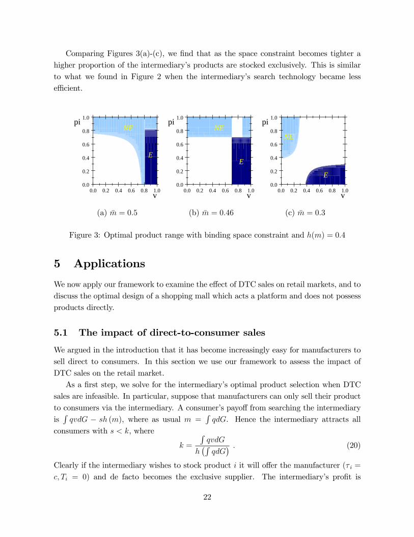
Comparing Figures 3(a)-(c), we �nd that as the space constraint becomes tighter ahigher proportion of the intermediary�s products are stocked exclusively. This is similarto what we found in Figure 2 when the intermediary�s search technology became lesse¢ cient.

NE

E

0.0 0.2 0.4 0.6 0.8 1.00.0

0.2

0.4

0.6

0.8

1.0

v

pi

(a) �m = 0:5

NE

E

0.0 0.2 0.4 0.6 0.8 1.00.0

0.2

0.4

0.6

0.8

1.0

v

pi

(b) �m = 0:46

NE

E

0.0 0.2 0.4 0.6 0.8 1.00.0

0.2

0.4

0.6

0.8

1.0

v

pi

(c) �m = 0:3

Figure 3: Optimal product range with binding space constraint and h(m) = 0:4

5 Applications

We now apply our framework to examine the e¤ect of DTC sales on retail markets, and todiscuss the optimal design of a shopping mall which acts a platform and does not possessproducts directly.

5.1 The impact of direct-to-consumer sales

We argued in the introduction that it has become increasingly easy for manufacturers tosell direct to consumers. In this section we use our framework to assess the impact ofDTC sales on the retail market.As a �rst step, we solve for the intermediary�s optimal product selection when DTC

sales are infeasible. In particular, suppose that manufacturers can only sell their productto consumers via the intermediary. A consumer�s payo¤ from searching the intermediaryisRqvdG � sh (m), where as usual m =

RqdG. Hence the intermediary attracts all

consumers with s < k, where

k =

RqvdG

h�RqdG

� : (20)

Clearly if the intermediary wishes to stock product i it will o¤er the manufacturer (� i =c; Ti = 0) and de facto becomes the exclusive supplier. The intermediary�s pro�t is

22

thereforeRq�F (k)dG, which is strictly positive for any stocking policy except q = 0.

The optimal product selection is reported in the following result:

Proposition 3 With no DTC sales, the intermediary stocks all the products with

� � �� �vF (k)

; (21)

where k > 0, � � 0 and � � 0 are de�ned in the appendix.

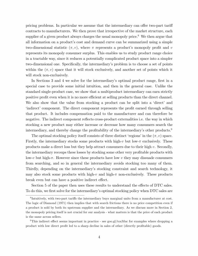
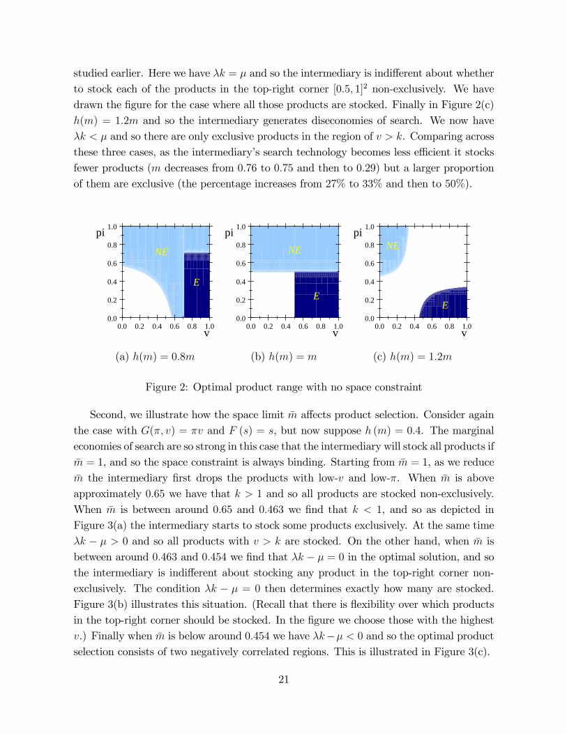
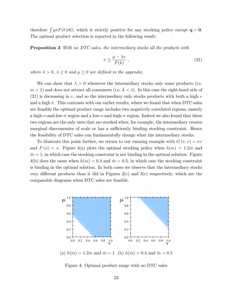
We can show that � > 0 whenever the intermediary stocks only some products (i.e.m < 1) and does not attract all consumers (i.e. k < �s). In this case the right-hand side of(21) is decreasing in v, and so the intermediary only stocks products with both a high vand a high �. This contrasts with our earlier results, where we found that when DTC salesare feasible the optimal product range includes two negatively correlated regions, namelya high-v-and-low-� region and a low-v-and-high-� region. Indeed we also found that thesetwo regions are the only ones that are stocked when, for example, the intermediary createsmarginal diseconomies of scale or has a su¢ ciently binding stocking constraint. Hencethe feasibility of DTC sales can fundamentally change what the intermediary stocks.To illustrate this point further, we return to our running example with G (�; v) = �v

and F (s) = s. Figure 4(a) plots the optimal stocking policy when h(m) = 1:2m and�m = 1, in which case the stocking constraint is not binding in the optimal solution. Figure4(b) does the same when h(m) = 0:4 and �m = 0:3, in which case the stocking constraintis binding in the optimal solution. In both cases we observe that the intermediary stocksvery di¤erent products than it did in Figures 2(c) and 3(c) respectively, which are thecomparable diagrams when DTC sales are feasible.

0.0 0.2 0.4 0.6 0.8 1.00.0

0.2

0.4

0.6

0.8

1.0

v

pi

(a) h(m) = 1:2m and �m = 1

0.0 0.2 0.4 0.6 0.8 1.00.0

0.2

0.4

0.6

0.8

1.0

v

pi

(b) h(m) = 0:4 and �m = 0:3

Figure 4: Optimal product range with no DTC sales

23

Now consider the impact of DTC sales on industry pro�ts:

Corollary 2 After DTC sales become feasible, manufacturer pro�t and total industrypro�t both increase, whilst the intermediary�s pro�t decreases.

Manufacturers clearly bene�t when DTC sales become feasible since they earn a pos-itive pro�t �F (v). However the intermediary�s pro�t is lower with DTC sales. To under-stand why, imagine that initially manufacturers can sell direct but then suddenly theycan�t. Even if the intermediary does not respond by changing its product selection, itspro�t increases because i) it no longer has to compensate manufacturers, and ii) weaklymore consumers search it, since they no longer have the option to buy direct. It is alsoeasy to show that the negative e¤ect of DTC sales on the intermediary is outweighed byits positive e¤ect on manufacturers, and so DTC sales raise industry pro�t.Interestingly, our model suggests that if an intermediary is to survive the threat posed

by DTC sales, it may need to qualitatively change the mix of products that it stocks.To illustrate this, consider again the examples in Figure 4. It turns out that if DTCsales become feasible but the intermediary wishes to stock (exclusively) the products inthe shaded regions, it will end up making a loss (pro�ts become respectively �0:027 and�0:036). However in both cases the intermediary can make positive pro�t by droppingmany of the high-v and high-� products that it previously stocked.Finally, the impact of DTC sales on consumer surplus and total welfare is di¢ cult to

investigate analytically since, as we have seen, the feasibility of DTC sales can signi�cantlychange the intermediary�s product selection. However in the examples we have studiedabove DTC sales improve both consumer surplus and total welfare. (In the example inFigure 4(a), DTC sales improve consumer surplus from 0:110 to 0:145 and total welfarefrom 0:329 to 0:413; in the example in Figure 4(b), DTC sales improve consumer surplusfrom 0:062 to 0:144 and total welfare from 0:186 to 0:406.) In addition, if �m is su¢ cientlysmall then DTC sales must improve both consumer surplus and total welfare since withoutDTC sales consumers are only able to buy very few products.

5.2 Shopping malls

Our framework can also shed light on the design of shopping malls. Suppose there isa unit mass of sellers each of which can either join a shopping mall and/or set up itsown independent shop in the same area. The shopping mall can host up to �m sellersand charges each of them a �xed fee. Consumers pay s to search an independent shopand h (m)� s to search a mall which contains m shops. The timing of o¤ers to join themall, pricing by sellers, and search decisions by consumers, are the same as in Section

24

2. (Notice that since the shopping mall acts as a platform, it does not set retail pricesdirectly.)This is isomorphic to our main model. Firstly, it is straightforward to see that seller

i will charge pmi wherever it sells its product. (We do not even need Lemma 1.) Henceour (�; v) representation remains valid. Secondly, consumers will search the mall if andonly if s < k where k was de�ned earlier in Lemma 3. Thirdly, sales of a product (�; v)at the mall generate a gross pro�t of �F (k). Therefore a seller with v < k will pay� [F (k)� F (v)] to join the mall, whilst a seller with v > k is willing to join the mall forfree if it also maintains an independent store elsewhere, but must be paid � [F (v)� F (k)]to exclusively join the mall. Consequently the mall owner�s pro�t is the same as inequation (13), and Proposition 2 characterizes which sellers join the mall.We can interpret sellers with v > k who are exclusive to the mall as �anchor stores�.

According to our model, the mall owner should subsidize anchor stores to encourage themto join. This is worthwhile because their presence attracts more consumers (i.e. increasesk), which allows the mall to charge a higher fee to other �non-anchor�stores. Consistentwith this, Gould et al (2005) show empirically that 73% of anchor stores pay zero rent (andthe mall developer often pays for things like development and maintenance costs). Evenamong stores which pay rents, anchor stores pay substantially lower rent than non-anchorstores ($4.13 vs $29.37 per square foot). They also �nd that adding more anchor storesto a mall leads to an increase in both the sales of, and the rents charged to, non-anchorstores.

6 Foundation of the (�; v) Product Space

Up to now we have characterized the intermediary�s optimal stocking policy in terms ofthe (�; v) space. In this section we explain how to construct the (�; v) space, and alsohow to interpret di¤erent points within in.We �rst discuss how to generate the (�; v) space. Suppose that demand for product

i can be written as Qi (pi) � Q (pi; �i) where �i is a vector of demand parameters. Wecan then let (�; c) denote the vector of product-speci�c parameters. Using the de�nitionsintroduced in equation (1), one can calculate �i = �(�i; ci) and vi = v(�i; ci), and thenderive the (�; v) space from the parameter space (�; c).34

34If products di¤er in exactly two parameters (like in the second example below), it is possible tohave a one-to-one correspondence between the parameter space and the (�; v) space. If products di¤erin more than two parameters (like in the �rst example below), generically each point in the (�; v) spacerepresents a continuum of di¤erent products. We can then let qE (�; v) and qNE (�; v) denote the fractionof products at point (�; v) which are respectively stocked exclusively and non-exclusively. Since all the

25

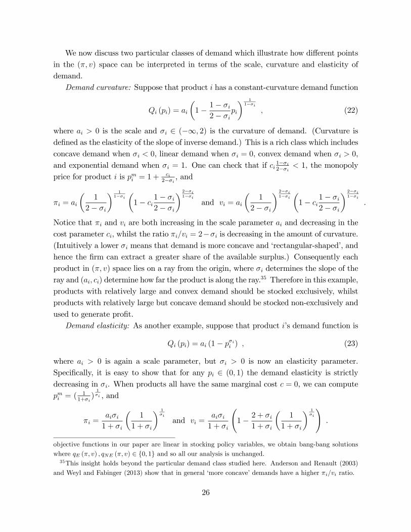
We now discuss two particular classes of demand which illustrate how di¤erent pointsin the (�; v) space can be interpreted in terms of the scale, curvature and elasticity ofdemand.Demand curvature: Suppose that product i has a constant-curvature demand function

Qi (pi) = ai

�1� 1� �i

2� �ipi

� 11��i

; (22)

where ai > 0 is the scale and �i 2 (�1; 2) is the curvature of demand. (Curvature isde�ned as the elasticity of the slope of inverse demand.) This is a rich class which includesconcave demand when �i < 0, linear demand when �i = 0, convex demand when �i > 0,and exponential demand when �i = 1. One can check that if ci 1��i2��i < 1, the monopolyprice for product i is pmi = 1 +

ci2��i , and

�i = ai

�1

2� �i

� 11��i

�1� ci

1� �i2� �i

� 2��i1��i

and vi = ai

�1

2� �i

� 2��i1��i

�1� ci

1� �i2� �i

� 2��i1��i

.

Notice that �i and vi are both increasing in the scale parameter ai and decreasing in thecost parameter ci, whilst the ratio �i=vi = 2��i is decreasing in the amount of curvature.(Intuitively a lower �i means that demand is more concave and �rectangular-shaped�, andhence the �rm can extract a greater share of the available surplus.) Consequently eachproduct in (�; v) space lies on a ray from the origin, where �i determines the slope of theray and (ai; ci) determine how far the product is along the ray.35 Therefore in this example,products with relatively large and convex demand should be stocked exclusively, whilstproducts with relatively large but concave demand should be stocked non-exclusively andused to generate pro�t.Demand elasticity: As another example, suppose that product i�s demand function is

Qi (pi) = ai (1� p�ii ) ; (23)

where ai > 0 is again a scale parameter, but �i > 0 is now an elasticity parameter.Speci�cally, it is easy to show that for any pi 2 (0; 1) the demand elasticity is strictlydecreasing in �i. When products all have the same marginal cost c = 0, we can computepmi = (

11+�i

)1�i , and

�i =ai�i1 + �i

�1

1 + �i

� 1�i

and vi =ai�i1 + �i

1� 2 + �i

1 + �i

�1

1 + �i

� 1�i

!.

objective functions in our paper are linear in stocking policy variables, we obtain bang-bang solutionswhere qE (�; v) ; qNE (�; v) 2 f0; 1g and so all our analysis is unchanged.35This insight holds beyond the particular demand class studied here. Anderson and Renault (2003)

and Weyl and Fabinger (2013) show that in general �more concave�demands have a higher �i=vi ratio.

26

Again both �i and vi are increasing in ai, whilst �i=vi is increasing in �i and thereforedecreasing in demand elasticity.36 (Intuitively when demand is more elastic the monopolyprice is lower and consumers enjoy a greater share of surplus.) Consequently in this exam-ple there is a one-to-one correspondence between (a; �) space and (�; v) space. Moreoverproducts with relatively large and elastic demands should be stocked exclusively, whilstproducts with relatively large and inelastic demand should be stocked non-exclusively toearn positive pro�t.

7 Extensions

In this section we return to the baseline model and discuss two extensions: one with a so-cial planner who aims to maximize total welfare, and the other with upstream competitionwhere each product is supplied by multiple manufacturers.

7.1 The socially optimal stocking policy

Consider the baseline model with DTC sales. We study the optimal product range ofa social planner that wishes to maximize total welfare (de�ned as the sum of industrypro�t and consumer surplus). The social planner chooses the stocking policy q, but hasno direct control over �rm pricing or how consumers search.Since the consumer search rule is the same as in Lemma 3, total welfare can be written

as

W (q) �Z�F (v) dG+�(q) +

Z k

0

u1 (s;q) dF (s) +

Z �s

k

u0 (s;q) dF (s) : (24)

The �rst term is pro�t earned by manufacturers. Note that a manufacturer earns �F (v)regardless of whether or not it sells via the intermediary. The second term is the inter-mediary�s pro�t, which we de�ned earlier in equation (13). The remaining two termsare consumer surplus. Consumers with s < k search the intermediary and earn u1 (s;q),which we de�ned in equation (10). Meanwhile consumers with s � k do not search theintermediary and so earn u0 (s;q), which we de�ned in equation (11). When some prod-ucts with v > k are stocked exclusively, consumers with s � k are made worse o¤ becausethey cannot buy all the products they would like to. At the same time, consumers withs < k are forced to buy some low-v products that ordinarily they would not purchase,and so depending on the strength of economies of search may or may not be better o¤.

36Notice that �i=vi > 1 for any �i > 0, and so the (�; v) space can only lie in half of the quadrant R2+.

27

The social planner wishes to maximize (24). We can solve its optimization problemusing the same techniques as we did earlier for pro�t maximization. We again use m =RqdG to denote the measure of products stocked by the intermediary.

Proposition 4 A su¢ cient condition for the socially optimal stocking policy to havem > 0 is that h ( ~m) � ~m for some ~m 2 (0; �m). The optimal policy is characterized asfollows (with k > 0, � � 0 and � � 0 de�ned in the appendix):(i) Products with v < k are stocked if and only if

� + v ��� �v �

R v0sdF (s)

F (k)� F (v) ; (25)

and it does not matter whether they are exclusive.(ii) Products with v > k are stocked exclusively if and only if

� + v �maxf�; �k +

R k0sdF (s)g � �v �

R v0sdF (s)

F (k)� F (v) : (26)

Of the remaining products with v > k, all of them are stocked non-exclusively if �k +R k0sdF (s) > �, some of them are stocked non-exclusively if �k+

R k0sdF (s) = �, and none

of them are stocked if �k +R k0sdF (s) < �.

It is socially optimal for the intermediary to stock a positive measure of products,provided that it generates (weak) economies of search for at least some ~m 2 (0; �m). Qual-itatively the welfare-optimal stocking policy is similar to what an unfettered intermediarywould choose. Firstly, exclusive products with v > k are again chosen to have low �, andproducts with v < k are chosen to have high �. Intuitively this is because, as we notedearlier, consumers do not take into account sellers�pro�t, and therefore search (and buy)too little from a welfare perspective. Demand for a product with v > k is further reducedwhen it is sold exclusively by the intermediary, but conversely demand for a product withv < k is increased when it is sold by the intermediary. Choosing the former products tohave low � minimizes the additional welfare loss, and choosing the latter to have a high� maximizes the welfare gains. Secondly, and mirroring Corollary 1 from earlier, whenthe stocking constraint is slack at the optimum all products with v > k are stocked ifh0(m) < 1, but only those with low � are stocked (and done so exclusively) if h0(m) > 1.37

We would now like to compare the stocking policies chosen by the intermediary andsocial planner. Unfortunately this is hard to do analytically, because in general (k; �; �)

37The indirect value of non-exclusively stocking a product with v > k is �k � � +R k0sdF (s), which

after solving for � simpli�es to [1� h0 (m)]��k +

R k0sdF (s)

�. Intuitively non-exclusivity of a product

leads consumers with s < k to buy it from the intermediary rather than from its manufacturer, and atthe margin this increases these consumers�search cost by h0 (m)� 1 units.

28

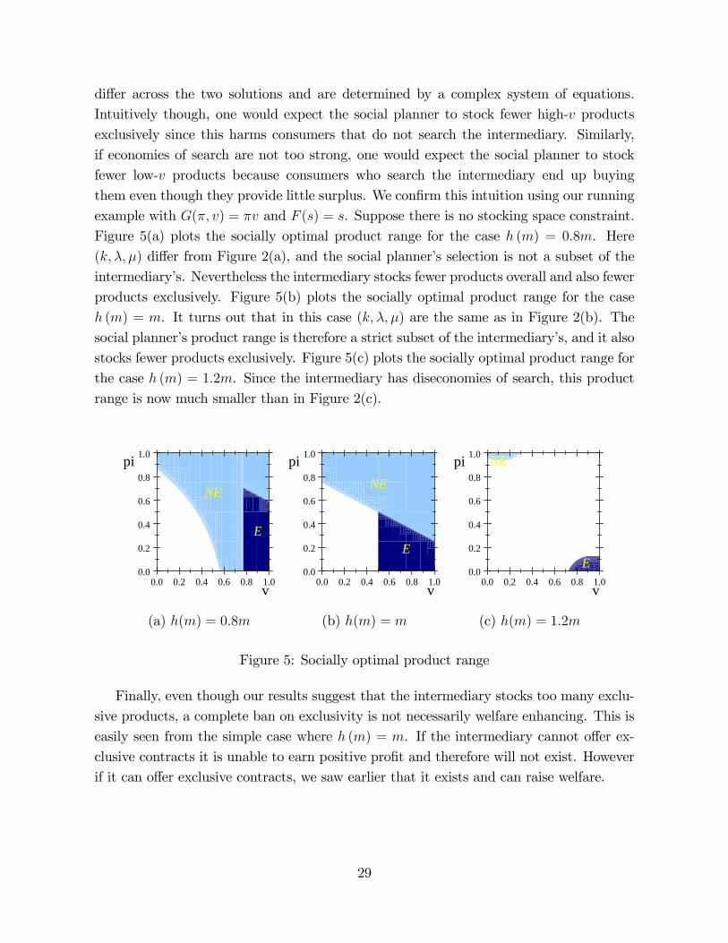
di¤er across the two solutions and are determined by a complex system of equations.Intuitively though, one would expect the social planner to stock fewer high-v productsexclusively since this harms consumers that do not search the intermediary. Similarly,if economies of search are not too strong, one would expect the social planner to stockfewer low-v products because consumers who search the intermediary end up buyingthem even though they provide little surplus. We con�rm this intuition using our runningexample with G(�; v) = �v and F (s) = s. Suppose there is no stocking space constraint.Figure 5(a) plots the socially optimal product range for the case h (m) = 0:8m. Here(k; �; �) di¤er from Figure 2(a), and the social planner�s selection is not a subset of theintermediary�s. Nevertheless the intermediary stocks fewer products overall and also fewerproducts exclusively. Figure 5(b) plots the socially optimal product range for the caseh (m) = m. It turns out that in this case (k; �; �) are the same as in Figure 2(b). Thesocial planner�s product range is therefore a strict subset of the intermediary�s, and it alsostocks fewer products exclusively. Figure 5(c) plots the socially optimal product range forthe case h (m) = 1:2m. Since the intermediary has diseconomies of search, this productrange is now much smaller than in Figure 2(c).

E

NE

0.0 0.2 0.4 0.6 0.8 1.00.0

0.2

0.4

0.6

0.8

1.0

v

pi

(a) h(m) = 0:8m

E

NE

0.0 0.2 0.4 0.6 0.8 1.00.0

0.2

0.4

0.6

0.8

1.0

v

pi

(b) h(m) = m

E

NE

0.0 0.2 0.4 0.6 0.8 1.00.0

0.2

0.4

0.6

0.8

1.0

v

pi

(c) h(m) = 1:2m

Figure 5: Socially optimal product range

Finally, even though our results suggest that the intermediary stocks too many exclu-sive products, a complete ban on exclusivity is not necessarily welfare enhancing. This iseasily seen from the simple case where h (m) = m. If the intermediary cannot o¤er ex-clusive contracts it is unable to earn positive pro�t and therefore will not exist. Howeverif it can o¤er exclusive contracts, we saw earlier that it exists and can raise welfare.

29

7.2 Upstream competition

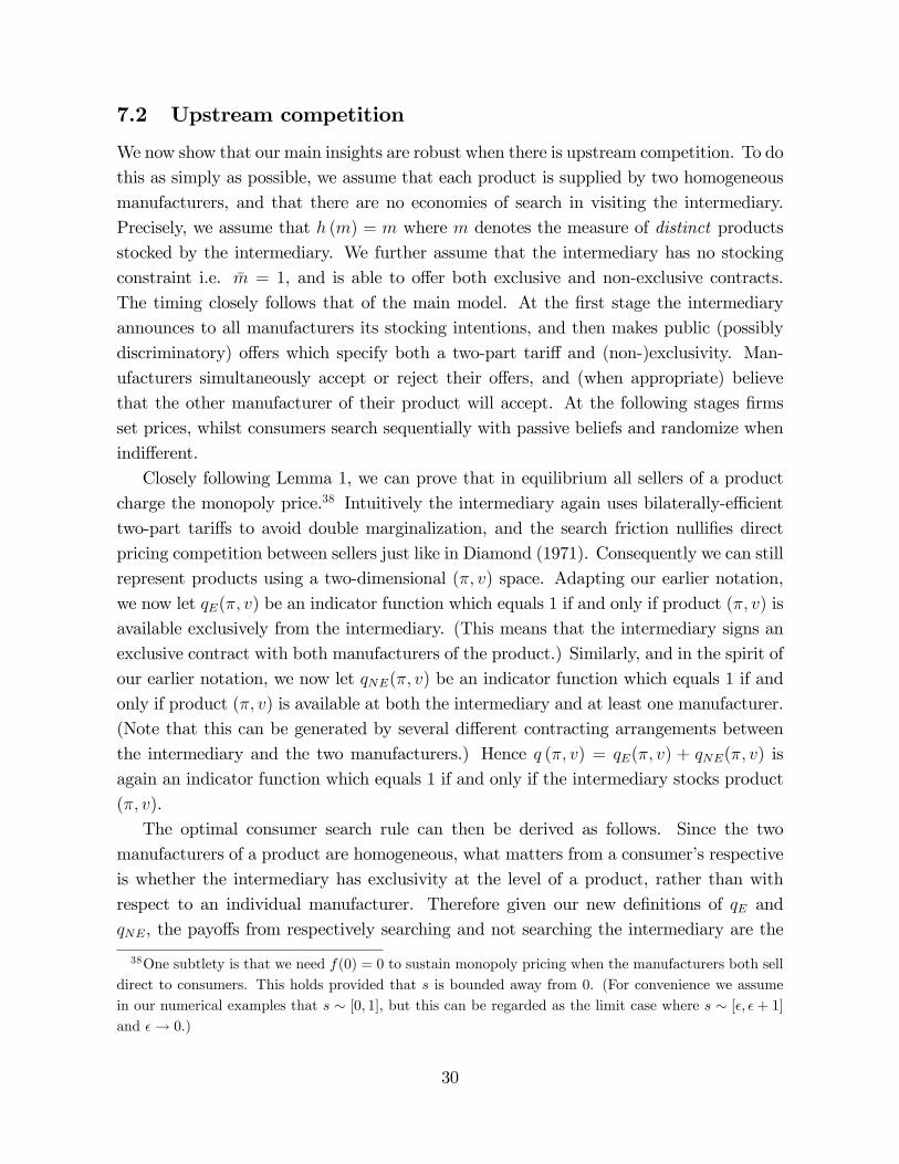
We now show that our main insights are robust when there is upstream competition. To dothis as simply as possible, we assume that each product is supplied by two homogeneousmanufacturers, and that there are no economies of search in visiting the intermediary.Precisely, we assume that h (m) = m where m denotes the measure of distinct productsstocked by the intermediary. We further assume that the intermediary has no stockingconstraint i.e. �m = 1, and is able to o¤er both exclusive and non-exclusive contracts.The timing closely follows that of the main model. At the �rst stage the intermediaryannounces to all manufacturers its stocking intentions, and then makes public (possiblydiscriminatory) o¤ers which specify both a two-part tari¤ and (non-)exclusivity. Man-ufacturers simultaneously accept or reject their o¤ers, and (when appropriate) believethat the other manufacturer of their product will accept. At the following stages �rmsset prices, whilst consumers search sequentially with passive beliefs and randomize whenindi¤erent.Closely following Lemma 1, we can prove that in equilibrium all sellers of a product

charge the monopoly price.38 Intuitively the intermediary again uses bilaterally-e¢ cienttwo-part tari¤s to avoid double marginalization, and the search friction nulli�es directpricing competition between sellers just like in Diamond (1971). Consequently we can stillrepresent products using a two-dimensional (�; v) space. Adapting our earlier notation,we now let qE(�; v) be an indicator function which equals 1 if and only if product (�; v) isavailable exclusively from the intermediary. (This means that the intermediary signs anexclusive contract with both manufacturers of the product.) Similarly, and in the spirit ofour earlier notation, we now let qNE(�; v) be an indicator function which equals 1 if andonly if product (�; v) is available at both the intermediary and at least one manufacturer.(Note that this can be generated by several di¤erent contracting arrangements betweenthe intermediary and the two manufacturers.) Hence q (�; v) = qE(�; v) + qNE(�; v) isagain an indicator function which equals 1 if and only if the intermediary stocks product(�; v).The optimal consumer search rule can then be derived as follows. Since the two

manufacturers of a product are homogeneous, what matters from a consumer�s respectiveis whether the intermediary has exclusivity at the level of a product, rather than withrespect to an individual manufacturer. Therefore given our new de�nitions of qE andqNE, the payo¤s from respectively searching and not searching the intermediary are the

38One subtlety is that we need f(0) = 0 to sustain monopoly pricing when the manufacturers both selldirect to consumers. This holds provided that s is bounded away from 0. (For convenience we assumein our numerical examples that s � [0; 1], but this can be regarded as the limit case where s � [�; �+ 1]and �! 0.)

30

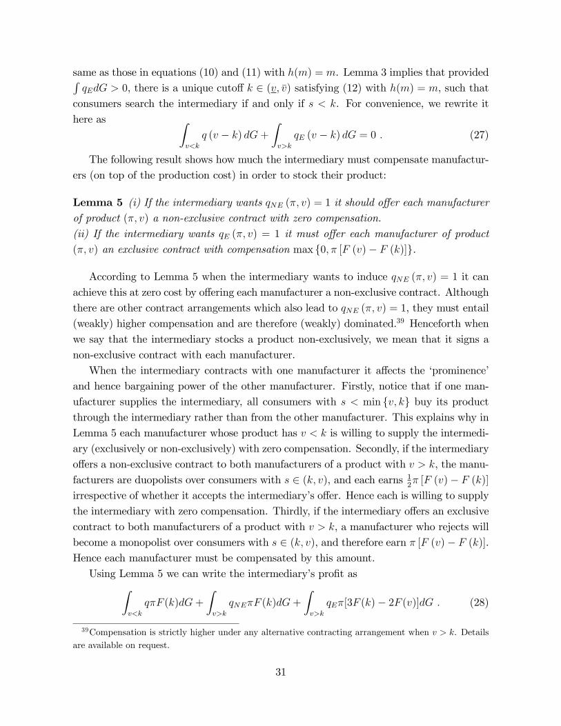
same as those in equations (10) and (11) with h(m) = m. Lemma 3 implies that providedRqEdG > 0, there is a unique cuto¤ k 2 (v; �v) satisfying (12) with h(m) = m, such that

consumers search the intermediary if and only if s < k. For convenience, we rewrite ithere as Z

v<k

q (v � k) dG+Zv>k

qE (v � k) dG = 0 : (27)

The following result shows how much the intermediary must compensate manufactur-ers (on top of the production cost) in order to stock their product:

Lemma 5 (i) If the intermediary wants qNE (�; v) = 1 it should o¤er each manufacturerof product (�; v) a non-exclusive contract with zero compensation.(ii) If the intermediary wants qE (�; v) = 1 it must o¤er each manufacturer of product(�; v) an exclusive contract with compensation max f0; � [F (v)� F (k)]g.

According to Lemma 5 when the intermediary wants to induce qNE (�; v) = 1 it canachieve this at zero cost by o¤ering each manufacturer a non-exclusive contract. Althoughthere are other contract arrangements which also lead to qNE (�; v) = 1, they must entail(weakly) higher compensation and are therefore (weakly) dominated.39 Henceforth whenwe say that the intermediary stocks a product non-exclusively, we mean that it signs anon-exclusive contract with each manufacturer.When the intermediary contracts with one manufacturer it a¤ects the �prominence�

and hence bargaining power of the other manufacturer. Firstly, notice that if one man-ufacturer supplies the intermediary, all consumers with s < min fv; kg buy its productthrough the intermediary rather than from the other manufacturer. This explains why inLemma 5 each manufacturer whose product has v < k is willing to supply the intermedi-ary (exclusively or non-exclusively) with zero compensation. Secondly, if the intermediaryo¤ers a non-exclusive contract to both manufacturers of a product with v > k, the manu-facturers are duopolists over consumers with s 2 (k; v), and each earns 1

2� [F (v)� F (k)]

irrespective of whether it accepts the intermediary�s o¤er. Hence each is willing to supplythe intermediary with zero compensation. Thirdly, if the intermediary o¤ers an exclusivecontract to both manufacturers of a product with v > k, a manufacturer who rejects willbecome a monopolist over consumers with s 2 (k; v), and therefore earn � [F (v)� F (k)].Hence each manufacturer must be compensated by this amount.Using Lemma 5 we can write the intermediary�s pro�t asZ

v<k

q�F (k)dG+

Zv>k

qNE�F (k)dG+

Zv>k

qE�[3F (k)� 2F (v)]dG : (28)

39Compensation is strictly higher under any alternative contracting arrangement when v > k. Detailsare available on request.

31

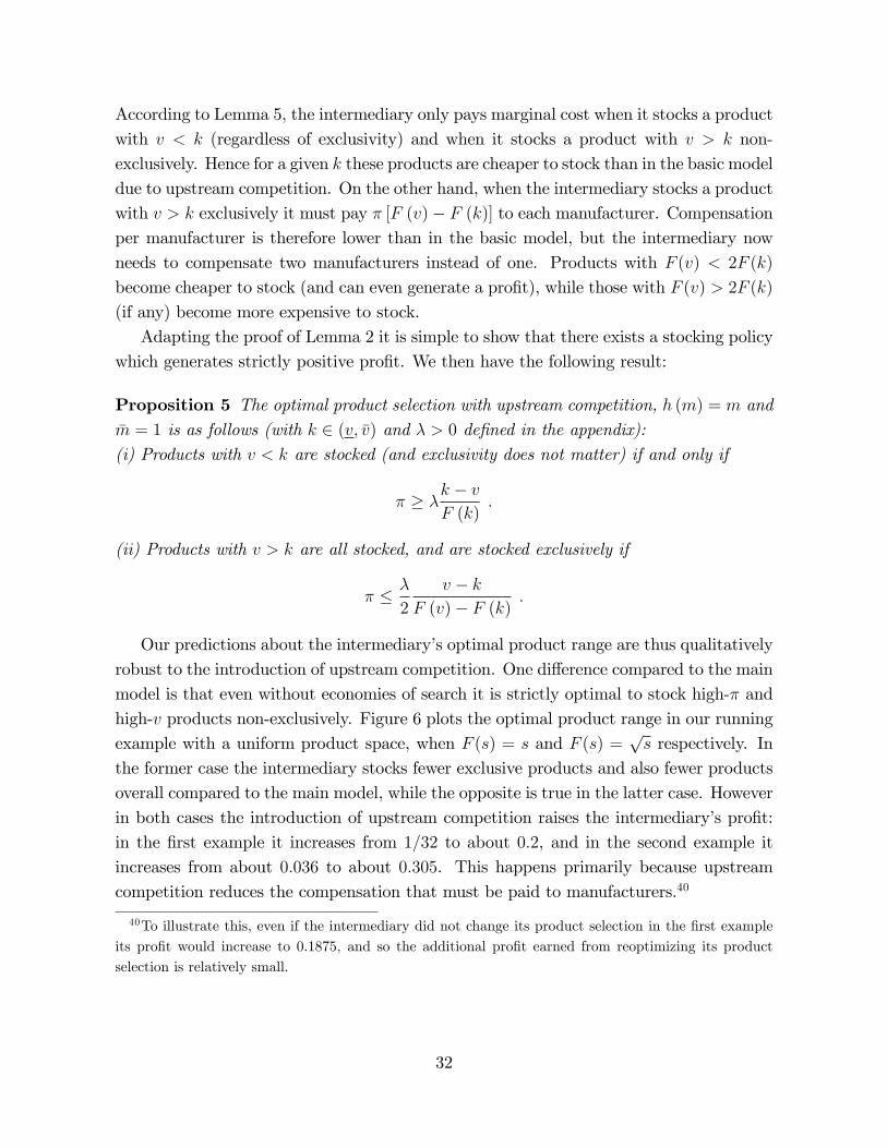
According to Lemma 5, the intermediary only pays marginal cost when it stocks a productwith v < k (regardless of exclusivity) and when it stocks a product with v > k non-exclusively. Hence for a given k these products are cheaper to stock than in the basic modeldue to upstream competition. On the other hand, when the intermediary stocks a productwith v > k exclusively it must pay � [F (v)� F (k)] to each manufacturer. Compensationper manufacturer is therefore lower than in the basic model, but the intermediary nowneeds to compensate two manufacturers instead of one. Products with F (v) < 2F (k)

become cheaper to stock (and can even generate a pro�t), while those with F (v) > 2F (k)(if any) become more expensive to stock.Adapting the proof of Lemma 2 it is simple to show that there exists a stocking policy

which generates strictly positive pro�t. We then have the following result:

Proposition 5 The optimal product selection with upstream competition, h (m) = m and�m = 1 is as follows (with k 2 (v; �v) and � > 0 de�ned in the appendix):(i) Products with v < k are stocked (and exclusivity does not matter) if and only if

� � �k � vF (k)

:

(ii) Products with v > k are all stocked, and are stocked exclusively if

� � �

2

v � kF (v)� F (k) :

Our predictions about the intermediary�s optimal product range are thus qualitativelyrobust to the introduction of upstream competition. One di¤erence compared to the mainmodel is that even without economies of search it is strictly optimal to stock high-� andhigh-v products non-exclusively. Figure 6 plots the optimal product range in our runningexample with a uniform product space, when F (s) = s and F (s) =

ps respectively. In

the former case the intermediary stocks fewer exclusive products and also fewer productsoverall compared to the main model, while the opposite is true in the latter case. Howeverin both cases the introduction of upstream competition raises the intermediary�s pro�t:in the �rst example it increases from 1=32 to about 0:2, and in the second example itincreases from about 0:036 to about 0:305. This happens primarily because upstreamcompetition reduces the compensation that must be paid to manufacturers.40

40To illustrate this, even if the intermediary did not change its product selection in the �rst exampleits pro�t would increase to 0:1875, and so the additional pro�t earned from reoptimizing its productselection is relatively small.

32

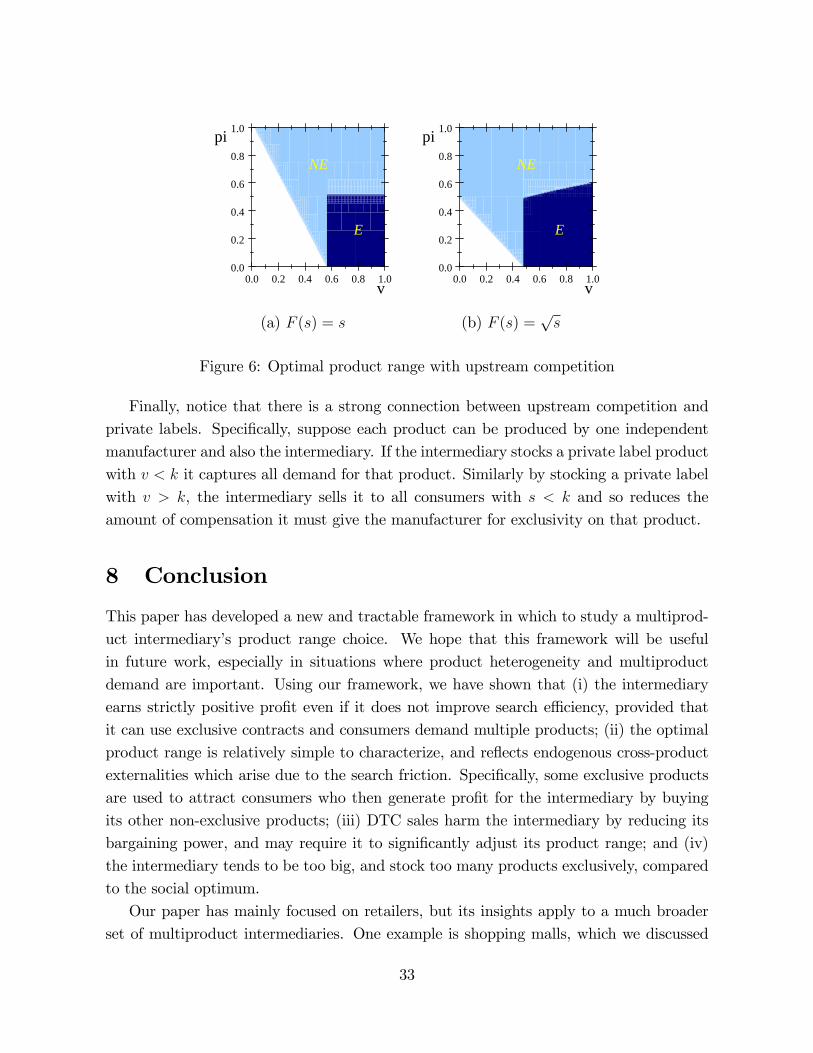
NE

E

0.0 0.2 0.4 0.6 0.8 1.00.0

0.2

0.4

0.6

0.8

1.0

v

pi

(a) F (s) = s

E

NE

0.0 0.2 0.4 0.6 0.8 1.00.0

0.2

0.4

0.6

0.8

1.0

v

pi

(b) F (s) =ps

Figure 6: Optimal product range with upstream competition

Finally, notice that there is a strong connection between upstream competition andprivate labels. Speci�cally, suppose each product can be produced by one independentmanufacturer and also the intermediary. If the intermediary stocks a private label productwith v < k it captures all demand for that product. Similarly by stocking a private labelwith v > k, the intermediary sells it to all consumers with s < k and so reduces theamount of compensation it must give the manufacturer for exclusivity on that product.

8 Conclusion

This paper has developed a new and tractable framework in which to study a multiprod-uct intermediary�s product range choice. We hope that this framework will be usefulin future work, especially in situations where product heterogeneity and multiproductdemand are important. Using our framework, we have shown that (i) the intermediaryearns strictly positive pro�t even if it does not improve search e¢ ciency, provided thatit can use exclusive contracts and consumers demand multiple products; (ii) the optimalproduct range is relatively simple to characterize, and re�ects endogenous cross-productexternalities which arise due to the search friction. Speci�cally, some exclusive productsare used to attract consumers who then generate pro�t for the intermediary by buyingits other non-exclusive products; (iii) DTC sales harm the intermediary by reducing itsbargaining power, and may require it to signi�cantly adjust its product range; and (iv)the intermediary tends to be too big, and stock too many products exclusively, comparedto the social optimum.Our paper has mainly focused on retailers, but its insights apply to a much broader

set of multiproduct intermediaries. One example is shopping malls, which we discussed

33

earlier in Section 5. Another pertinent example is TV platforms. Traditionally, contentproviders mainly reached viewers through TV subscription services. However in recentyears Disney, HBO, ESPN and several others have launched (or committed to launch)DTC channels.41 Our model can be applied to understand how this might a¤ect theindustry: the manufacturers in our model can be interpreted as content providers, whilstthe search friction could be interpreted more broadly as encompassing the costs of �nding,subscribing to, and paying for various services.42 Our model then provides implicationsabout, for example, what channels a cable TV company will carry and how it is a¤ectedby the introduction of DTC channels. Another example where our framework could befruitfully applied is international trade, because intermediaries play an important role inhelping domestic manufacturers to export.43 In that case foreign importers are like theconsumers in our model, whilst trade frictions are similar to our search cost. Dependingon how easy it is for individual manufacturers to export on their own (which is like DTCin our model), they may choose to sell via an intermediary. Hence by modifying our modelone could obtain insights about which products should be exported, and by whom.Finally, we believe that our paper opens up some promising avenues for future research.

Firstly, we have focused on a monopoly intermediary. It would be interesting to allowfor multiple intermediaries, and study how competition between them (or a merger oftwo intermediaries) shapes their optimal product range. Secondly, we have assumed thateach product has only one manufacturer or two homogenous manufacturers. It would beinteresting to investigate the case where each product has several manufacturers, each ofwhom produces a di¤erentiated variety. This would make it possible to study both theintermediary�s optimal breadth (i.e. how many di¤erent types of product to stock) anddepth (i.e. how many varieties of a particular product to stock).

Appendix

Proof of Lemma 1. (i) Consider an equilibrium in which a set AM of productsare sold only by their manufacturers, a set AE of products are stocked exclusively by theintermediary, and a set ANE of products are stocked non-exclusively by the intermediary.Let pl be the equilibrium price of product l 2 AM , pj be the equilibrium price of product

41See goo.gl/7rZ4LW for details on Disney and ESPN, and goo.gl/8Mwf2i for details on HBO�s �HBONow�service.42See goo.gl/7eQGek for arguments why these costs can be much lower when content is bundled rather

than sold direct.43See e.g. Bernard et al (2010) and Ahn et al (2011) for empirical evidence on trade intermediaries in

the US and China respectively.

34

j 2 AE, and pi;M and pi;I be the equilibrium price of product i 2 ANE at its manufacturerand the intermediary, respectively. Note that if pi;I > pi;M it is possible that a consumervisits the intermediary which stocks product i but buys product i from its manufacturer.However if pi;I � pi;M it is impossible that in equilibrium a consumer visits both theintermediary and the manufacturer.(i-1) As in the case of no intermediary, it is easy to see pl = pml for l 2 AM given our

informational assumption.(i-2) We then show pj = pmj for j 2 AE. Suppose the wholesale price of prod-

uct j is � j. The hold-up logic implies that the intermediary must charge p�j (� j) =argmaxp (p� � j)Qj (p). (Note that p�j (cj) = pmj .) Since the intermediary makes a take-it-or-leave-it o¤er, it will optimally o¤er a lump-sum fee Tj = �jF (vj)�(� j � cj)Qj(p�j (� j))�� to manufacturer j, where � is the measure of consumers who visit the intermediary andwhich only depends on the expected surplus from visiting the intermediary. (In particu-lar, given consumers do not observe the contract details, � is independent of the actualwholesale price � j.) Hence the intermediary�s pro�t from stocking product j exclusivelyis

� � [p�j (� j)� � j]Qj(p�j (� j))� Tj = � ��p�j (� j)� cj

�Qj(p

�j (� j))� �jF (vj) : (29)

This is maximized at p�j (� j) = pmj such that the intermediary should o¤er a wholesaleprice � j = cj.(i-3) We �nally show pi;I = pi;M = pmi for i 2 ANE. The proof consists of a few steps.Step 1: pi;M � pmi .If in contrast pi;M > pmi in equilibrium, then reducing pi;M slightly will be a pro�table

deviation. First, the number of consumers who buy product i from respectively theintermediary and manufacturer i does not change. For those consumers who visit theintermediary and buy product i there, they do not observe manufacturer i�s price reductionand so still buy from the intermediary. For those consumers who visit the intermediary�rst and then come to manufacturer i, they will be surprised by the price reduction butwill still buy from manufacturer i as originally planned. The number of such consumersdoes not increase since their search decision is based on expected equilibrium prices. Forthose who visit manufacturer i �rst, their initial plan must be to buy product i at themanufacturer (otherwise they would have no reason to visit it). Again a private pricereduction will not increase the number of such consumers, and once they arrive they buyas planned (given passive beliefs). Second then, manufacturer i earns strictly more pro�tfrom its direct sales to consumers, and earns the same pro�t from sales made through theintermediary.Step 2: pi;M = pmi .

35

If in contrast pi;M < pmi in equilibrium, then increasing pi;M slightly will be a pro�tabledeviation. Consider the following two cases separately:(a) pi;I > pi;M . Consider a slight increase to pi;M + " < minfpi;I ; pmi g. For those who

visit the intermediary �rst and then come to manufacturer i (based on the expected price),they will be surprised by manufacturer i�s price increase but will still buy from it sinceits price remains strictly below pi;I . For those who visit manufacturer i �rst (again, basedon the expected price), they will buy as planned given the new price is still lower thanpi;I . Therefore, the number of consumers who buy at manufacturer i remains unchanged,but the pro�t from each of them is now higher.(b) pi;I � pi;M . For those who visit the intermediary �rst, they will not come to

manufacturer i according to their beliefs, so they are irrelevant for a private price devi-ation. For those who plan to visit manufacturer i, they must not visit the intermediaryon equilibrium path. If pi;M is slightly increased, will some of them switch to visitingthe intermediary? The answer is no, because in our continuum framework this singleprice deviation has a zero-measure impact on the consumer surplus from not visiting theintermediary and so will not change consumer search behavior.44 Therefore again a smallprice increase will improve manufacturer i�s pro�t.Step 3: pi;I � pmi .Suppose in contrast pi;I > pmi (= pi;M) in equilibrium. In this case, there are two

possible types of consumer who buy product i. Let �i;I be the measure of consumerswho buy i at the intermediary, and let �i;M be the measure of consumers who buy i atmanufacturer i. (Some of the latter consumers may visit the intermediary but buy fromthe manufacturer.) Consider two cases separately:(a) � i � ci. Then a small reduction of pi;I will be a pro�table deviation. Slightly

decreasing pi;I will weakly increase �i;I . At the same time the intermediary makes ahigher pro�t from each such consumer given that p�i (� i) � pmi < pi;I .(b) � i > ci. In this case we argue that a deviation to p0i;I = pmi (together with an

adjustment of the two-part tari¤) will be pro�table. In the hypothetical equilibrium, wemust have

Ti + �i;I � (� i � ci)Qi(pi;I) + �i;M � �i = �iF (vi) :

44With a discrete number of products, the same result holds by a slightly di¤erent argument. Considera consumer who is ex ante indi¤erent between whether or not to visit the intermediary. If she visitsmanufacturer i and �nds pi;M slightly higher than expected, will she now want to visit the intermediary?Since the cost of visiting the manufacturer is already sunk, she actually would have a strict preferencefor not visiting the intermediary if pi;M remained the same as expected. Therefore the same is true ifpi;M is only slightly higher than she expected.

36

Then the intermediary�s pro�t from product i is

�i;I � (pi;I � � i)Qi(pi;I)� Ti = �i;I � (pi;I � ci)Qi(pi;I) + �i;M � �i � �iF (vi) :

If pi;I is reduced to pmi , (pi;I � ci)Qi(pi;I) will increase to �i, the per-consumer monopolypro�t, and �i;I + �i;M will increase at least weakly.45 Then the pro�t must be improved.Step 4: pi;I = pmi .Suppose in contrast pi;I < pmi (= pi;M) in equilibrium. Then if a consumer visits the

intermediary, she will not visit manufacturer i. In this case it is then impossible that� i � ci. Otherwise the intermediary could improve its pro�t from product i by raisingpi;I slightly. (Note that this deviation does not a¤ect the number of consumers who visitthe intermediary, and once they arrive they will still buy product i at the intermediaryas long as pi;I is still below pi;M .)Now consider the possibility of � i < ci. Then we must have pi;I = p�i (� i) in an

equilibrium. Then a deviation to � 0i = ci and p0i;I = pmi will be pro�table. (Given thecontract details are unobservable to consumers, such a deviation will not a¤ect the numberof consumers who visit the intermediary and buy i.)This completes the proof for pi;I = pi;M = pmi for i 2 ANE.(ii) The equilibrium two-part tari¤ for product j 2 AE has been proved in (i-2)

above. Now consider the equilibrium two-part tari¤ for product i 2 ANE. It is easy tosee that � i < ci is impossible. Otherwise the intermediary would have an incentive toreduce its price for product i to p�i (� i). However, we cannot rule out the possibility of� i > ci (together with Ti such that manufacturer i�s pro�t is �iF (vi)). The reason isthat if the intermediary raises its price for product i above pmi , some consumers who visitthe intermediary and initially planned to buy i there may then switch to buying frommanufacturer i. If the number of such consumers is large enough (which requires f(s) tobe large enough for small s), the intermediary does not dare to raise its price.Fortunately, this indeterminacy of the contract details does not matter for our subse-

quent analysis of optimal product selection. Suppose in an equilibrium � i 6= ci for somei 2 ANE. The lump-sum fee Ti satis�es

Ti + �i;I � (� i � ci)Qi(pi;I) + �i;M � �i = �iF (vi) :

45In fact, it can be shown that �i;I+�i;M remains unchanged. The consumers who buy product i can bedivided into three groups: some don�t visit the intermediary and buy i at manufacturer i; some visit theintermediary but buy i at manufacturer i; the rest visit the intermediary and buy i there. The deviationdoes not a¤ect the �rst group. The deviation may a¤ect the distribution of consumers between the secondand the third group, but does not a¤ect the total number of consumers who visit the intermediary whichonly depends on the expected prices.

37

Note that given the monopoly pricing result, �i;I is also the number of consumers who visitthe intermediary which is denoted by �I . Then the intermediary�s pro�t from stockingproduct i is

�I � (pmi � � i)Qi(pmi )� Ti = �I � (pmi � ci)Qi(pmi ) + �i;M � �i � �iF (vi)= �i [�I � (F (vi)� �i;M)] : (30)

Since consumer search and purchase behavior only depends on the retail prices, thispro�t is the same as if � i = ci. Therefore, without loss of generality, we can focus on acontracting outcome with � i = ci.

Proof of Lemma 2. (i) We �rst show that the intermediary can make a positivepro�t by stocking a positive measure of products. Consider two interior points in: (�1; ~v)and (�2; ~v) with �1 > �2. Let A1 = [�1 � �; �1] � [~v � �; ~v] and A2 = [�2; �2 +�(v)] �[~v; ~v + �], where �(v) is uniquely de�ned for each v 2 [~v; ~v + �] byZ �1

�1��g (�; 2~v � v) d� =

Z �2+�(v)

�2

g (�; v) d� : (31)

Convexity of implies that we have A1; A2 � for su¢ ciently small � � 0 and � > 0.Notice that �(v) is constructed in such a way that for each v in A2, the mass of productsstocked is the same as that of the �mirror�valuation 2~v � v in A1. This implies thatthe average v of the products in A1 [ A2 is always ~v, and so a consumer will visit theintermediary, when it stocks A = A1 [ A2, if and only if s < ~v.Fix a su¢ ciently small � such that �1 � � > �2 + �(v) for all v 2 [~v; ~v + �]. The

intermediary�s pro�t from stocking A = A1 [ A2 is

�(�) =

Z ~v

~v��

Z �1

�1��� [F (~v)� F (v)] dG+

Z ~v+�

~v

Z �2+�(v)

�2

� [F (~v)� F (v)] dG : (32)

Straightforward calculations reveal that �(0) = �0 (0) = 0. However,

�00 (0) = f (~v) [

Z �1

�1���g (�; ~v) d� �

Z �2+�(~v)

�2

�g (�; ~v) d�]

> f (~v) [(�1 � �)Z �1

�1��g (�; ~v) d� � (�2 +�(~v))

Z �2+�(~v)

�2

g (�; ~v) d�]

= f (~v) [(�1 � �)� (�2 +�(~v))]Z �1

�1��g (�; ~v) d� > 0 ;

where the second equality used (31) evaluated at v = ~v. Therefore, �(�) > 0 for � in aneighborhood of 0.

38

(ii) We then show that stocking all the products is not the most pro�table strategy. Letv̂ =

RvdG. Consider B1 = [�1 � �; �1]� [v̂; v̂ + �] and B2 = [�2; �2 +�(v)]� [v̂ � �; v̂],

where �1 > �2, and where �(v) is uniquely de�ned for each v 2 [v̂ � �; v̂] byZ �1

�1��g (�; 2v̂ � v) d� =

Z �2+�(v)

�2

g (�; v) d� : (33)

Convexity of implies that B1; B2 � for su¢ ciently small � � 0 and � > 0. Similarlyas above, the average v of the products in B1 [ B2 is always v̂, and so the average v inA = n (B1 [B2) is v̂ as well. Then a consumer will visit the intermediary, when it stocksA = n (B1 [B2), if and only if s < v̂.Fix a su¢ ciently small � such that �1 � � > �2 + �(v) for all v 2 [v̂ � �; v̂]. The

intermediary�s pro�t from stocking A = n (B1 [B2) is

�̂ (�) = �̂�Z v̂+�

v̂

Z �1

�1��� [F (v̂)� F (v)] dG�

Z v̂

v̂��

Z �2+�(v)

�2

� [F (v̂)� F (v)] dG ;

where �̂ = �̂ (0) is the pro�t from stocking . Simple calculations reveal that �̂0 (0) = 0.However, similar as in (i),

�̂00 (0) = f (v̂) [

Z �1

�1���g (�; v̂) d� �

Z �2+�(v̂)

�2

�g (�; v̂) d�] > 0

by using (33) evaluated at v = v̂. Therefore, �̂ (�) > �̂ for � in a neighborhood of 0.

Proof of Lemma 3. The di¤erence in payo¤ between (10) and (11) is

�(s) =

ZqvdG� h(

ZqdG)s�

Zv>s

qNE (v � s) dG : (34)

(We have used q�qE = qNE.) Notice that �(0) � 0, and �(s) is weakly concave because

�0(s) = �h(ZqdG) +

Zv>s

qNEdG

is weakly decreasing in s.(i) No consumer visits the intermediary (i.e. k = 0) if and only if �(s) � 0 for all

s > 0. A necessary and su¢ cient condition for this is �(0) = 0 and �0 (0) � 0, which isequivalent to the conditions stated in the lemma.(ii) All consumers visit the intermediary (i.e. k > �s) if and only if �(s) > 0 for all

s > 0. A necessary and su¢ cient condition for this is �(�s) > 0, which simpli�es to thecondition in the lemma.(iii) Finally in all other cases, �(s) > 0 for s in a neighborhood of 0, and �(�s) � 0, so

given that �(s) is weakly concave consumers use a cut-o¤ strategy. Consumers strictly

39

prefer visiting the intermediary if they have s < k, where k solves �(k) = 0. (12) is justa rewriting of �(k) = 0.

Proof of Lemma 4. Recall the areas A1 and A2 that were de�ned in the proof ofLemma 2, and let v� (�) be the unique solution to

~m =

ZA1[A2

dG+

Zv>v�(�)

dG :

Notice that since ~m is bounded away from 1 and is convex, we can �nd ~v su¢ cientlyclose to v, and � > 0 su¢ ciently small, such that for � > 0 su¢ ciently small we have bothA1; A2 � and v� (�) > ~v + �.Suppose the intermediary stocks products inA1 andA2 exclusively and stocks products

with v > v� (�) non-exclusively. Firstly notice that for any � > 0 we have k � ~v. To seethis, note that by the de�nition of �(s) in equation (34) we have

�(~v) =

ZqvdG� h(

ZqdG)~v �

Zv>~v

qNE (v � ~v) dG

�ZA1[A2

vdG� ~vZA1[A2

dG = 0 ;

where the inequality uses h�RqdG

�= h ( ~m) � ~m, and the �nal equality follows since

A1 [ A2 is constructed to have average valuation ~v. The hypotheses of Lemma 3(iii) aresatis�ed, and the proof of that lemma shows that�(~v) � 0 implies k � ~v. Secondly, recallthat non-exclusive products with v < k earn positive pro�t, and non-exclusive productswith v > k earn zero pro�t. Therefore since k � ~v the intermediary�s pro�t is weaklylarger than in equation (32) in the proof of Lemma 2, and in that proof we showed thatthis pro�t is strictly positive for some � > 0.

Proof of Proposition 2. As a preliminary step, the slackness conditions for thespace constraint are �( �m � m) = 0 and � � 0. Hence, � = 0 if m < �m in the optimalsolution, and � is irrelevant if m = �m since in that case the binding space constraint isthe same as (15). Also, when the intermediary makes a strictly positive pro�t, we musthave k > 0 so that some consumers visit it.First, we characterize the optimal product selection for given parameters (k; �; �).

From (17) it is clear that for v < k, q = 1 if and only if

� [F (k)� F (v)] + �v � � � 0, � � �� �vF (k)� F (v) ; (35)

and the exclusivity arrangement does not matter. From (17) it is also clear that for v > k,qE = 1 if and only if

� [F (k)� F (v)] + �v � � � maxf0; �k � �g , � � maxf�k; �g � �vF (k)� F (v) : (36)

40

When the opposite is true, qNE = 1 if �k � � > 0, qNE = 0 if �k � � < 0, and theintermediary is indi¤erent between qNE = 0 and qNE = 1 if �k � � = 0. (In the thirdcase, there is �exibility over which products should be stocked, but the selection has tosatisfy �k � � = 0 as we explain more below.)Second, we give the conditions for determining the parameters. It is useful to consider

a few cases separately:(a) Suppose the optimal solution has k < �s.46 Then k satis�es (14). Since k is interior,

the �rst-order condition of (17) with respect to k gives

� = f(k)

Rv<k

q�dG+Rv>k

qE�dG

h(m)�Rv>k

qNEdG> 0 : (37)

(Notice that � > 0 since � and k de�ned in (12) share the same denominator.) If m < �m

in the optimal solution, then � = 0 as we have pointed out and so the �rst-order conditionof (17) with respect to m gives

� = �kh0 (m) � 0 ; (38)

and (k; �; �;m) jointly solve equations (14), (15), (37) and (38). If m = �m in the optimalsolution, � is irrelevant as we have explained. Note that if m = �m < 1 then (k; �; �)jointly solve equations (14), (15) and (37) with m replaced by �m everywhere, and we canconclude that � � 0.47 Note that if insteadm = �m = 1 then � does not matter so withoutloss of generality we can set � = 0, and (k; �) jointly solve equations (14) and (37) withm replaced by �m.48 (Regardless of whether (16) binds or not, when �k � � = 0 we havean additional equation, but this determines the measure of products with v > k that arestocked non-exclusively.)(b) Suppose the optimal solution has k > �s.49 Then there is no region of v > k given

our focus on v � s. The value of k now does not a¤ect the product selection which ischaracterized by (35) with F (k) = 1. As stated in the text � = 0 in this case. We can alsodeduce that m = �m in the optimal solution. Suppose to the contrary that m < �m: (38)implies � = 0, and so (17) is increasing in q for all products which contradicts m < �m. Ifm = �m < 1 in the optimal solution then � � 0 is determined by �m =

RqdG, where q = 1

46According to Lemma 3, a su¢ cient condition for k < s in the optimal solution is thatRqvdG=h(

RqdG) < s for any q, or equivalently maxx

R vxvdG=h(

R vxdG) < s. This condition is easy

to hold when economies of search are weak and s� v.47Notice that if to the contrary � < 0, then by (35) all products should be stocked, which contradicts

m = �m < 1. The same argument applies in parts (b) and (c) below when m = �m < 1.48Note that the righthand side of (35) is weakly negative and that �k � � � 0, so this is consistent

with m = 1. A similar argument applies in part (b) below when m = �m = 1.49According to Lemma 3, k > �s in the optimal solution requires

RqvdG > h ( �m) �s.

41

for the products satisfying (35). If instead m = �m = 1 then � does not matter and so wecan without loss of generality set � = 0.(c) Suppose the optimal solution has k = �s.50 Again, there is no region of v > k in

this case. If m < �m in the optimal solution, (�; �;m) jointly solve equations (14) withk = s, (15) and (38). If m = �m < 1 in the optimal solution, � and � � 0 jointly solve(14) with k = s and �m =

RqdG, where q = 1 for the products satisfying (35). If instead

m = �m = 1 then � does not matter so we can set � = 0, and any � � 0 is consistentwith the right hand side of (35) being weakly negative such that every product is indeedstocked.

Proof of Corollary 1. This is immediate from cases (a) and (c) in the proof ofProposition 2. (Note that we must have m = �m in case (b).)

Proof of Proposition 3. We only give a sketch of the proof since it is very similarto that of Proposition 2. As before we treat m =

RqdG as a constraint and set up the

(Kuhn-Tucker) Lagrange function

L =Zq(�F (k) + �v � �)dG� �kh(m) + �m+ �( �m�m) ; (39)

where we again set � = 0 if k > �s in the optimal solution.For given parameters (k; �; �) it is clear from (39) that the intermediary will stock

product (�; v) if and only if

�F (k) + �v � � � 0, � � �� �vF (k)

:

To determine the parameters it is again useful to consider a few cases separately. (a)Suppose the optimal solution has k < s. If m < �m in the optimal solution, we have � = 0,� = �kh0(m), and (k; �;m) solve

k =

RqvdG

h(m), � = f(k)

Rq�dG

h(m), m =

ZqdG : (40)

If m = �m in the optimal solution, � is irrelevant. If �m < 1 then (k; �; �) solve (40) withm = �m. If instead �m = 1 then without loss of generality we can set � = 0, and (k; �)solve (40) with m = 1 and without the m equation. (b) Suppose the optimal solution hask > s. Then as before we have � = 0 and m = �m in the optimal solution. If �m < 1 then� is determined by �m =

RqdG. If instead �m = 1 we can without loss of generality set

� = 0. (c) Suppose the optimal solution has k = s. If m < �m in the optimal solution,

50According to Lemma 3, k = �s in the optimal solution requiresRqvdG = h (m) �s.

42

� = �kh0(m) and (�;m) solve (40) with k = s and without the � equation. If insteadm = �m < 1 then (�; �) solve (40) with k = s and m = �m and without the � equation. Ifinstead m = �m = 1 then � solves the �rst equation in (40) with k = s, � = 0 and m = 1.

Proof of Corollary 2. First, note that without DTC sales each manufacturer earns0, whereas with DTC sales each manufacturer earns �F (v), so total manufacturer pro�tstrictly increases. Let qD and qND be the optimal stocking policies respectively with andwithout DTC sales. Second, consider total industry pro�t and suppose DTC sales arefeasible. Notice that if

�qE = q

ND;qNE = 0then compared with the case where DTC

is unavailable: i) equations (34) and (20) imply that k is the same, and therefore industrypro�t on products with qND = 1 is also the same, but ii) industry pro�t is higher ongoods with qND = 0. However in general the intermediary chooses qD 6= qND, so itspro�t is higher than under

�qE = q

ND;qNE = 0whilst manufacturer pro�t is the same.

Thus industry pro�t is (weakly) higher when DTC sales are feasible. Third, consider theintermediary�s pro�t and suppose DTC sales are infeasible. Notice that if the intermediarystocks a product if and only if qD = 1 then i) k is weakly higher because using equation(34) �

�kND

�� 0 where kND is the solution to equation (20), and ii) compensation paid

to manufacturers is weakly lower. Hence intermediary pro�t must be (weakly) higherwhen DTC sales are infeasible.

Proof of Proposition 4. The proof that the social optimum has m > 0 uses asimilar technique to the one in the proof of Lemma 4 and so is omitted. To characterizethe optimal stocking policy, substitute the expressions for �(q), u1 (s;q) and u0 (s;q)into equation (24) to get

W (q) =

Z(1� q)

Z v

0

(� + v � s)dF (s)dG+Zq(� + v)F (k)dG

�h(m)Z k

0

sdF (s) +

Zv>k

qNE

Z v

k

(� + v � s)dF (s)dG : (41)

Maximizing W (q) is the same as maximizing W (q)�W (0) i.e. the welfare improve-ment due to the intermediary. We therefore maximize W (q) � W (0) subject to theconstraints (14), (15) and (16), and let �, � and � be the associated Lagrange multipliers.

43

After some algebraic manipulations, we can write the Lagrange function as follows:

L =Zv<k

q

�(� + v) [F (k)� F (v)] + �v � �+

Z v

0

sdF (s)

�| {z }

[1]

dG

+

Zv>k

8>>><>>>:qE�(� + v) [F (k)� F (v)] + �v � �+

Z v

0

sdF (s)

�| {z }

[2]

+ qNE

��k � �+

Z k

0

sdF (s)

�| {z }

[3]

9>>>=>>>; dG� h(m)

��k +

Z k

0

sdF (s)

�+ �m+ �( �m�m) : (42)

This problem is similar to the pro�t-maximizing one. As before � = 0 if m < �m in theoptimal solution, and � is irrelevant if m = �m.For given parameters (k; �; �), products with v < k will be stocked if [1] � 0, which

leads to (25). In this region, the exclusivity arrangement does not matter. Products withv > k will be stocked exclusively if [2] � maxf0; [3]g, which leads to (26). When theopposite is true, they will be stocked non-exclusively if [3] > 0.We now explain how to determine the parameters (k; �; �). Here we only consider the

case where the optimal solution has k < �s. (The case of k > s or k = s can be easilydealt with like we did in the proof of Proposition 2.) Taking the �rst order condition of(42) with respect to k and then using equation (12) to cancel terms, we obtain

� = f(k)

Rv<k

q�dG+Rv>k

qE�dG

h(m)�Rv>k

qNEdG> 0 : (43)

This is the same as equation (37) from the proof of Proposition 2. If m < �m in theoptimal solution, then � = 0 and so the �rst-order condition of (42) with respect to mgives

� = h0(m)

��k +

Z k

0

sdF (s)

�� 0 ; (44)

Then (k; �; �;m) jointly solve equations (14), (15), (43) and (44). If m = �m in theoptimal solution, � is irrelevant as we have explained. Note that if m = �m < 1 then(k; �; �) jointly solve equations (14), (15) and (43) with m replaced by �m everywhere, andwe can conclude that � � 0 as in the proof of Proposition 2. If instead m = �m = 1 then� does not matter so without loss of generality we can set � = 0, and (k; �) jointly solveequations (14) and (43) with m replaced by �m.

Proof of Proposition 5. The intermediary maximizes (28) subject to the search

44

constraint (27). The Lagrangian function of this optimization problem is

L =

Zv<k

q [�F (k) + � (v � k)] dG+Zv>k

qNE�F (k) dG

+

Zv>k

qE f� [3F (k)� 2F (v)] + � (v � k)g dG : (45)

The intermediary must stock some products exclusively otherwise from Lemma 2 noconsumer will search it and it will earn zero pro�t. From equation (27) the optimummust have k 2 (v; �v), and so taking the �rst order condition of (45) with respect to kyields

� = f (k)

Rv<k

q�dG+Rv>k

qNE�dG+ 3Rv>k

qE�dGRv<k

qdG+Rv>k

qEdG; (46)

from which we deduce � > 0. Equations (27) and (46) jointly determine k and �, and theremainder of the proposition follows immediately from equation (45).

References

Adams, W., and J. Yellen (1976): �Commodity Bundling and the Burden ofMonopoly,�Quarterly Journal of Economics, 90(3), 475�498.

Ahn, J., A. Khandelwal, and S. Wei (2011): �The Role of Intermediaries in Facili-ating Trade,�Journal of International Economics, 84(1), 73�85.

Anderson, S., and R. Renault (2003): �E¢ ciency and Surplus Bounds in CournotCompetition,�Journal of Economic Theory, 113(2), 253�264.

(2006): �Advertising Content,�American Economic Review, 96(1), 93�113.

Asker, J., and H. Bar-Isaac (2017): �Vertical Information Restraints: Pro- and Anti-Competitive Impacts of Minimum Advertised Price Restrictions,�mimeo.

Bernard, A., B. Jensen, S. Redding, and P. Schott (2010): �Wholesalers andRetailers in US Trade,�American Economic Review, 100(2), 408�413.

Biglaiser, G. (1993): �Middlemen as Experts,�RAND Journal of Economics, 24(2),212�223.

Biglaiser, G., and F. Li (2018): �Middlemen: the good, the bad, and the ugly,�RANDJournal of Economics, 49(1), 3�22.

45

Bronnenberg, B. (2017): �Innovation and Distribution: A General Equilibrium Modelof Manufacturing and Retailing,�mimeo.

Chen, Y., and M. Riordan (2013): �Pro�tability of Product Bundling,�InternationalEconomic Review, 54(1), 35�57.

Diamond, P. (1971): �A Model of Price Adjustment,� Journal of Economic Theory,3(2), 156�168.

Gehrig, T. (1993): �Intermediation in Search Markets,� Journal of Economics andManagement Strategy, 2(1), 97�120.

Gould, E., P. Pashigian, and C. Prendergast (2005): �Contracts, Externalities,and Incentives in Shopping Malls,�Review of Economics and Statistics, 87(3), 411�422.

Hagiu, A., and B. Jullien (2011): �Why Do Intermediaries Divert Search?,�RANDJournal of Economics, 42(2), 337�362.

Janssen, M., and S. Shelegia (2015): �Consumer Search and Double Marginaliza-tion,�American Economic Review, 105(6), 1683�1710.

Kaplan, G., G. Menzio, L. Rudanko, and N. Trachter (2016): �Relative PriceDispersion: Evidence and Theory,�mimeo.

Kok, G., M. Fisher, and R. Vaidyanathan (2015): �Assortment Planning: Re-view of Literature and Industry Practice,�in Retail Supply Chain Management, ed. byN. Agrawal, and S. Smith. Springer.

Lizzeri, A. (1999): �Information Revelation and Certi�cation Intermediaries,�RANDJournal of Economics, 30(2), 214�231.

McAfee, P. (1995): �Multiproduct Equilibrium Price Dispersion,�Journal of EconomicTheory, 67(1), 83�105.

McAfee, P., J. McMillan, and M. Whinston (1989): �Multiproduct Monopoly,Commodity Bundling, and Correlation of Values,�Quarterly Journal of Economics,104(2), 371�383.

Rayo, L., and I. Segal (2010): �Optimal Information Disclosure,�Journal of PoliticalEconomy, 118(5), 949�987.

Rhodes, A. (2015): �Multiproduct Retailing,�Review of Economic Studies, 82(1), 360�390.

46

Rhodes, A., and J. Zhou (2017): �Consumer Search and Retail Market Structure,�Management Science, forthcoming.

Rubinstein, A., and A. Wolinsky (1987): �Middlemen,�Quarterly Journal of Eco-nomics, 102(3), 581�593.

Shelegia, S. (2012): �Multiproduct Pricing in Oligopoly,� International Journal ofIndustrial Organization, 30(2), 231�242.

Shevchenko, A. (2004): �Middlemen,�International Economic Review, 45(1), 1�24.

Spiegler, R. (2000): �Extracting Interaction-Created Surplus,�Games and EconomicBehavior, 30(1), 142�162.

Spulber, D. (1996): �Market Making by Price-Setting Firms,� Review of EconomicStudies, 63(4), 559�580.

(1999): Market Microstructure: Intermediaries and the Theory of the Firm.Cambridge University Press.

Stigler, G. (1968): �A Note on Block Booking,� in The Organization of Industry, ed.by G. Stigler. University of Chicago Press.

Stiglitz, J. (1979): �Equilibrium in Product Markets with Imperfect Information,�American Economic Review, 69(2), 339�345.

Weyl, G., and M. Fabinger (2013): �Pass-Through as an Economic Tool: Principlesof Incidence under Imperfect Competition,�Journal of Political Economy, 121(3), 528�583.

Zhou, J. (2014): �Multiproduct Search and the Joint Search E¤ect,�American EconomicReview, 104(9), 2918�2939.

47